Optimal taxation and spending in general competitive ...darp.lse.ac.uk/PapersDB/Judd_(JPubE_99).pdf · Optimal taxation and spending in general competitive ... K.L.Judd / Journal

Journal of Public Economics 71 (1999) 1–26

Optimal taxation and spending in general competitivegrowth models

a ,b ,*Kenneth L. JuddaHoover Institution, Stanford, CA, 94305, USA

bNational Bureau of Economic Research, City, USA

Received 30 June 1995; accepted 21 April 1998

Abstract

We find that the optimal long-run tax on capital income is zero even if the capital stockdoes not converge to a steady state nor to a steady state growth rate. The optimal tax onhuman capital is also zero if human capital is not a final good, but the long-run wage tax isnot generally zero. We argue that ‘‘consumption’’ tax proposals, such as the Flat Tax, arenot consumption taxes, and are biased against human capital. 1999 Elsevier ScienceS.A. All rights reserved.

Keywords: Optimal taxation; Human capital; Growth; Consumption taxation

JEL classification: H21

1. Introduction

This paper explores the proposition that the optimal long-run tax on capitalincome is zero. In contrast with earlier studies, we distinguish between human andphysical capital, we include public goods, we allow general, nonstationaryproduction functions, and we do not assume convergence of dynamic equilibriumto any kind of steady state. The general result we find is that the optimal tax onphysical capital is zero on average except for an initial period. Furthermore, thiszero-average-tax result holds also for human capital if it has no final consumption

*Tel.: 11-650-723-5866; fax: 11-650-723-1687; e-mail: [email protected]

0047-2727/99/$ – see front matter 1999 Elsevier Science S.A. All rights reserved.PI I : S0047-2727( 98 )00054-1

2 K.L. Judd / Journal of Public Economics 71 (1999) 1 –26

value, but that labor income will generally be taxed in the long-run. This can beaccomplished by taxing all labor income but subsidizing human capital inputs. Weargue that all these results follow from optimal commodity taxation theory.

There have been many analyses which argue for a zero long-run capital incometax rate. Early arguments, such as Atkinson and Sandmo (1980); Auerbach (1979),and Diamond (1973), relied heavily on separability assumptions and identicalagents in each cohort. Judd (1985) found a zero optimal long-run capital incometax rate for steady states of competitive dynamic general equilibrium withheterogeneous infinitely-lived agents and nonseparable preferences. Others haveexplored taxation issues in models of unbounded growth. Eaton (1981) showedthat capital income taxation reduces the steady state growth rate and Hamilton(1987) demonstrated that asymmetric treatment of different forms of capital has ahigh welfare cost. Jones et al. (1997) and Bull (1993) argued that the zero-taxresult also holds for all factor income, labor as well as both human and physicalcapital, in models generalizing the Eaton model. Jones et al. (1997) also argue thatrevenue constraints may lead to taxation of capital income in the long-run. Weshow that these results arise from special and unrealistic assumptions they make.Also, this paper proves its results without making any convergence assumptions;instead we include public goods to the analysis and find that assuming nondegen-erate expenditures on public goods serves as a substitute for assuming conver-gence.

One general problem with this literature is the lack of economic intuition. Theanalyses in Judd (1985); Bull (1993), and Jones et al. (1997) are presented informal ways not clearly connected with basic principles of optimal taxation; inparticular, they strongly use the assumption of convergence to a steady state. Otheranalyses have focussed on special long-run dynamic features. For example,Auerbach (1979) conjectured that the zero optimal capital income tax result arisesfrom the infinite long-run elasticity of savings in representative agent models withseparable utility. Judd (1985) showed that this long-run elasticity property is notrelevant since the same long-run zero tax results even if the long-run savingelasticity is finite and differs across individuals; however, no alternative intuitionwas offered.

In this paper, we ignore simple dynamic features such as the steady-statebehavior or long-run elasticities, and instead put the zero long-run tax results onmore economically appealing foundations. To do this, we look to the commoditytax literature. Two results from that literature apply here; first, the optimality ofuniform taxation with separable and sufficiently symmetric utility, and, second, theprohibition against intermediate good taxation derived in Diamond and Mirrlees,1971. Our methods generalize previous work and tie the results to the commoditytax literature, a change which helps us understand why we often find that theaverage tax rate on capital income is zero in the optimal policy.

The issues examined here are central to current policy debates in the U.S. A keyfeature of consumption tax proposals, such as those described in Bradford (1986);

K.L. Judd / Journal of Public Economics 71 (1999) 1 –26 3

Hall and Rabushka (1995); McClure and Zodrow (1996), and Weidenbaum (1997)is the zero effective tax rate on income from new physical capital investments;however, none propose a true consumption tax. The difference arises because theywould not give human capital investments the same treatment they advocate forphysical capital investment. These ‘‘consumption tax’’ proposals essentiallyadvocate reducing the tax burden of physical capital but increasing the tax burdenof some human capital investments, and do so without offering any explanation forthis policy preference over a true consumption tax. The analysis below argues forsymmetric treatment of physical and human capital, a type of ‘‘level playing field’’argument which follows the Diamond–Mirrlees case against intermediate goodtaxation.

2. Basic intuition from optimal commodity tax theory

The optimal factor taxation literature has generally derived its results throughdynamic optimization methods in ways which do not illustrate the underlyingeconomic logic. In contrast, the results of the optimal commodity taxationliterature are stated in more intuitive ways. In this section we review two basicoptimal commodity taxation ideas—the inverse elasticity rule and the nontaxationof intermediate goods—and show how these ideas can be used to understand theoptimal factor taxation results.

We first consider a simple problem wherein the optimal commodity tax isuniform. Suppose that we have an additively separable, isoelastic utility functionover n commodities,

n

U 5Ou(c )ii50

Also assume that good 0 is the numeraire and is untaxed, p is the consumer pricei

of good i, q is the producer price of good i, and the government’s problem is toi

tax the n commodities so as to maximize U subject to a revenue constraint. Theinverse elasticity rule says that the optimal tax rates on goods i±0, ( p 2q ) /q ,i i i

1are equal across all commodities . Such a tax structure would produce a uniformdistortion between the marginal rate of substitution and the marginal rate oftransformation between each good c and the numeraire. More precisely, for alli

i±0,

u9(c )i]]MRS ; 5 p 5 (1 1 t)q ; (1 1 t)MRT (1)i,0 i i i,0u9(c )0

1See Atkinson and Stiglitz (1972) for a discussion of the inverse elasticity rule, and its generalvalidity in the case of separable utility.


Note that this implies that there is no distortion in the choice between goods i, j±0since (1) implies MRS 5MRT . This result also generalizes to the case where wei, j i, j

have n untaxed ‘‘leisures’’, l , i50, 1,...,n, and the utility function is a weightedi

sum, as in

n nc lU 5O w u(c ) 1O w v(l ) (2)i i i i

i50 i50

Suppose next that the indices i refer to the same commodity at different dates, andc lthat the weights w and w in (2) equal the discount factor for utility in period ii i

relative to period 0. From general equilibrium theory we know that the Arrow–Debreu model applies to this dynamic context; similarly, so does the ‘‘static’’

2commodity tax literature . The resulting optimal uniform tax policy createsuniform MRS /MRT distortions between the untaxed good and every other good.

Income taxation implies a pattern of distortions across consumption and leisureat various dates. For example, if we have an asset at time 0 which we liquidated attime t to finance consumption, then a tax on the investment income essentiallytaxes consumption at time t. However, income taxation cannot perfectly implementcommodity taxation. The difference lies in the initial time periods. For example, ifthe interest rate is 10% per period, then a 100% tax on interest income results inthe cost of period 1 consumption equalling one unit of period 0 consumption andimplies an effective commodity tax rate of 11% on period 1 consumption. Anyhigher interest tax income rate is avoidable by just holding wealth in the form of

3zero interest rate assets, such as money . Therefore, this 11% commodity tax ratebetween periods 0 and 0 is the highest possible commodity tax which can beimplemented by an income tax system, even though a higher commodity tax ratemay be desirable. The upper bounds on implementable commodity tax ratesindicates that there will be an initial period of 100% interest tax rates; after thisinitial period, the optimal plan would presumably return to the desirable uniformpattern of distortion between these goods and period 0 consumption.

While this is all stated in commodity tax terms, the principle can be readilytranslated into income taxation. We can sharply illustrate the points in a simple

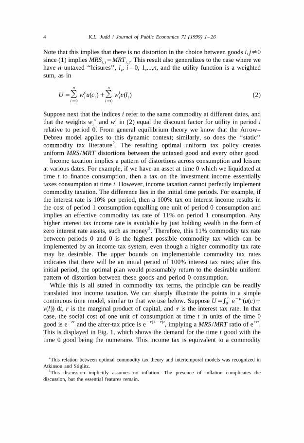
` 2r tcontinuous time model, similar to that we use below. Suppose U 5e e (u(c)10

v(l)) dt, r is the marginal product of capital, and t is the interest tax rate. In thatcase, the social cost of one unit of consumption at time t in units of the time 0

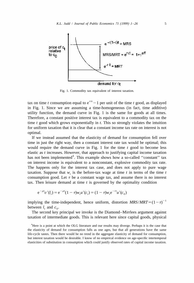
2rt 2r(12t )t rt tgood is e and the after-tax price is e , implying a MRS /MRT ratio of e .This is displayed in Fig. 1, which shows the demand for the time t good with thetime 0 good being the numeraire. This income tax is equivalent to a commodity

2This relation between optimal commodity tax theory and intertemporal models was recognized inAtkinson and Stiglitz.

3This discussion implicitly assumes no inflation. The presence of inflation complicates thediscussion, but the essential features remain.


Fig. 1. Commodity tax equivalent of interest taxation.

rt ttax on time t consumption equal to e 21 per unit of the time t good, as displayedin Fig. 1. Since we are assuming a time-homogeneous (in fact, time additive)utility function, the demand curve in Fig. 1 is the same for goods at all times.Therefore, a constant positive interest tax is equivalent to a commodity tax on thetime t good which grows exponentially in t. This so strongly violates the intuitionfor uniform taxation that it is clear that a constant income tax rate on interest is notoptimal.

If we instead assumed that the elasticity of demand for consumption fell overtime in just the right way, then a constant interest rate tax would be optimal; thiswould require the demand curve in Fig. 1 for the time t good to become lesselastic as t increases. However, that approach to justifying capital income taxation

4has not been implemented . This example shows how a so-called ‘‘constant’’ taxon interest income is equivalent to a nonconstant, explosive commodity tax rate.The happens only for the interest tax case, and does not apply to pure wagetaxation. Suppose that w is the before-tax wage at time t in terms of the time tt

consumption good. Let t be a constant wage tax, and assume there is no interesttax. Then leisure demand at time t is governed by the optimality condition

2r t 2r t 2rte v9(l ) 5 e (1 2 t)w u9(c ) 5 (1 2 t)w e u9(c )t t t t 0

21implying the time-independent, hence uniform, distortion MRS /MRT5(12t)between l and c .t 0

The second key principal we invoke is the Diamond–Mirrlees argument againsttaxation of intermediate goods. This is relevant here since capital goods, physical

4Here is a point at which the OLG literature and our results may diverge. Perhaps it is the case thatthe elasticity of demand for consumption falls as one ages, but that all generations have the samelife-cycle tastes. Then there would be no trend in the aggregate elasticity of demand for consumption,but interest taxation would be desirable. I know of no empirical evidence on age-specific intertemporalelasticities of substitution in consumption which could justify observed rates of capital income taxation.


and human, are intermediate goods. In fact, income taxation is equivalent to salestaxation of intermediate goods. This can be seen by noting, for example, that a100% sales tax on capital equipment is equivalent to a 50% tax on the income flowfrom capital equipment. Since intermediate good taxation will generally put aneconomy on the interior of its production possibilities frontier, capital incometaxation is likely to produce similar factor distortions, particularly if there aremany capital goods. Therefore, an optimal tax structure would tax only finalgoods.

These two principles together have strong implications for optimal tax policy inboth the static and dynamic contexts. In the next sections we will make all thismore precise, exploring how far we can apply these ideas to dynamic generalequilibrium models.

3. A simple aggregate model

We begin by presenting the main results in a simple aggregate model. We willexamine models more general than the usual ones. In particular, we will allowsocial increasing returns to scale. We will then examine generalizations involvingother types of capital.

3.1. The Representative Agent’s Problem

We assume that the representative agent’s utility function depends on consump-tion, c, labor supply, n, and a vector of government expenditures, g, and that theutility function is globally concave in the individual decisions, but not necessarilyin g. We first explore the individual’s dynamic problem. If we let A denote an

¯ ¯individual’s assets, r the after-tax return on A, and w the after-tax wage rate, thenthe individual’s maximization problem is

`2r tmax E e u(c, n, g) dtc,n (3)0

] ]~s.t. A 5rA 1wn 2 c

¯ ¯His current value Hamiltonian is u(c, n, g)1l(rA1wn2c) where l is the currentvalue shadow price of A. The costate equation for l is

]~l 5 l(r 2r) (4)

5The first-order conditions for the choices of c and n are

¯0 5 u 2 l, u 5 2 lw (5)c n

5We drop arguments of u and other functions to prevent notational clutter when those arguments areclear from context.


3.2. Representative Agent versus Alternative Models

At this point we should point out the reasons why we choose an infinite-lived,representative agent model over an overlapping generations (OLG) model, theapproach taken, for example, in Atkinson and Sandmo (1980), or a model withagent heterogeneity. In the OLG literature, some results revolve around the relativesocial weight put on successive generations versus the period-to-period discount-ing of an individual. Here, there will be no such conflicts and the results are drivenpurely by efficiency considerations.

Furthermore, the typical OLG model assumes agents live for only two periods.This specification makes it difficult to match empirical data concerning therelevant elasticities to the two-period OLG model given the high amount ofintertemporal aggregation present in the latter. Also, intertemporal nonseparabilityplays a critical role in the typical OLG analysis. As Judd (1985) emphasizes, thezero-tax result is far less sensitive to assumptions concerning tastes in therepresentative agent case than in the OLG case. Finally, most OLG analysisexamines the steady state nature of optimal policy, whereas we will not makesteady state assumptions and will derive more robust dynamic implications. This iseasiest to do in the representative agent framework.

It is unclear how much heterogeneous tastes and productivity would alter theresults. Judd (1985) shows that the zero taxation of capital is optimal even in somemodels with substantial agent heterogeneity and redistributive motives. In general,this paper abstracts from redistributive issues, both inter- and intragenerational.

The purpose of this paper is to pursue the logic of the zero-tax result for capitaland examine its relevance for human capital. This exercise can be accomplishedmost cleanly in our simple infinitely-lived, representative agent model withintertemporally separable utility. In particular, the commodity tax literature, suchas Diamond and Mirrlees, presumes an Arrow–Debreu general equilibriumframework, whereas the Arrow–Debreu analysis does not apply to OLG models.Since we want to investigate the intuitions of commodity tax theory in a dynamicframework, it is most natural to do in the representative agent framework. Both theOLG and representative agent extremes are flawed approximations of reality. Iconjecture that the infinite-life model is a better approximation of reality than thetwo-period OLG model, but that conjecture remains to be confirmed. Further workis needed to see how robust these results are to alternative demographicspecifications, empirically reasonable intertemporal utility functions, and dis-tributional concerns.

3.3. Social Problem

The optimal tax problem for our representative agent model is to maximize theutility of the representative agent subject to the dynamic revenue constraint and


keeping the agent on his demand and supply curves. This is summarized in theoptimal control problem

`2r t

] ]max E e u(c, n, g) dtc,n, g,w,r0

~s.t. k 5 f(k, n, g, t) 2 c 2 g~ ¯l 5 l(r 2 r ) (6)~ ¯ ¯ ¯B 5 rB 2 ( f(k, n, g, t) 2 rk 2 wn 2 g)

lim uBu , `t→`

¯ ¯0 5 u 2 l, 0 5 u 1 lw, r $ 0c n

where we include time t in the production function f(k, n, g, t) so as to allow6exogenous growth factors. The Hamiltonian for this problem is

¯H 5 u(c, n, g) 1 f ( f(k, n, g, t) 2 c 2 g) 1 f l(r 2 r )k l

¯ ¯ ¯ ¯1 m(rB 2 ( f(k, n, g, t) 2 rk 2 wn 2 g)) 1 f (u 2 l) 1 f (u 1 lw )c c n n

¯1 nr (7)

where f is the social marginal value of private capital k, f is the social marginalk l

value of l, f is the social marginal value of the requirement that the planner’sc

consumption choice be on the representative agents intertemporal demand curve,f is the social marginal value of the requirement that consumption, labor supply,n

and net wage be consistent with the representative agent’s preferences, n is the¯Kuhn–Tucker multiplier on the requirement that r $0, and m is the social

marginal utility value of debt B. We will sometimes refer to the capital and labor¯ ¯income tax rates, t and t , which are defined by (12t )f 5r and (12t )f 5w.K L K k L n

¯ ¯The first-order conditions for c, n, r, and w are

0 5 u 2 f 1 f u 1 f u (8)c k c cc n cn

0 5 u 1 f f 2 m( f 2 w) 1 f u 1 f u (9)n k n n c cn n nn

0 5 mn 1 f l (10)n

0 5 2 f l 1 m(B 1 k) 1 n (11)l

We assume several public goods; for each one we have the first-order condition

6I will follow the standard approach to this problem. The problem statement in (6) and theHamiltonian in (7) are not correct since the revenue constraint in (6) really should be an integralconstraint stating that the present value of B equals discounted future surpluses. It can be shown thatthe solution to the correct isoparametric formulation of (6) does reduce to the solution we displaybelow; we illustrate that procedure later in our analysis of human capital.


0 5 u 1 (f 2 m)( f 2 1) 1 f u 1 f u (12)g k g c cg n ng

The costate equations are

~ ¯f 5 f (r 2 f ) 2 m(2f 1 r )k k k k

¯~m 5 m(r 2 r ) (13)

~ ¯ ¯f 5 f r 2 f 1 wfl l c n

There are a few items which can be immediately determined. First, l.0 from (5).7Second, m #0 since the planner can always give bonds to agents . Third, if some

public good g has no effect on tastes or technology but must be nonnegative, thenslackness condition complementary to (12) implies f 2m $0; this is essentiallyk

saying that the government can buy goods and costlessly destroy them, a freedisposal assumption. All other public goods will be assumed to have interiorsolutions to (12), using an Inada condition if necessary. We summarize this in theLemma 1.

Lemma 1. If bonds can be given to private agents, and the government iscapable of free disposal of goods, then at all times t,

l . 0, m # 0, f 2 m $ 0 (14)k

We proceed under the assumptions made in Lemma 1.

3.4. Evolution of Multipliers

We next derive important intermediate results concerning the evolution of thecritical shadow prices m, l, and f . The first important item to note is thek

constancy of the ratio 2m /l.0, which we denote m. Lemma 2 holds since (4)d m] ]and (13) imply ( ) 5 0.dt l

Lemma 2. At all t, m;2m /l52m /l is constant on the solution to (6 ).0 0

The quantity m$0 is the wealth equivalent of the cost to the social objective ofone more dollar of initial debt; it is the marginal social cost of funds, also knownas the marginal excess burden of taxation. We will use m and 2m /l inter-changeably.

We will proceed under the usual assumption that the optimal policy isdeterministic. This is not an innocent assumption since (6) is not a concave

7Technically, this requires adding a policy instrument, bond transfers to agents, which we have notincluded above. Since they are unlikely to be used and their only function is to show m #0, we avoidsome notational clutter and do not include such bond transfers explicitly.


problem, and randomization is part of the solution for some optimal taxationproblems. The assumption of a deterministic policy is reasonable in many cases,particularly if m is small: we know that the solution is deterministic if m50 andone suspects that an implicit function theorem is valid for m near 0. We follow theusual practice of ignoring these technical details.

¯Most of our results concern the structure of the optimal policy when the r .0constraint is slack. At such times, (11) implies f 52m(B1k), the differentiationl

of which implies

d~ ] ¯ ¯f 5 2 m (B 1 k) 5 2 m(r(B 1 k) 1 wn 2 c)l dt

When this is combined with the costate Eqs. (13) and first-order conditions (10,~11) to eliminate f , we findl

~¯ ¯2 m(r(B 1 k) 1 wn 2 c) 5 fl

¯ ¯ ¯5 2 rm(B 1 k) 1 f 2 f w ⇒ 2 m(wn 2 c)c n

¯5 f 2 f wc n

However, (10) shows that f 5mn; therefore f 5mc. Combining this solution forn c

f with (8) and (10) yields Lemma 3.c

¯Lemma 3. When the r $0 constraint in (6 ) is slack, then

0 5 u 2 l 1 m(cu 1 nu ) (15)c k cc cn

l 2 f cu 1 nuk cc cn]] ]]]5 (16)

m uc

f 2 m cu 1 nuk cc cn]] ]]]5 1 1 m 1 1 (17)S Dl uc

Because of its critical importance, we define a composite multiplier

f 2 mk]]L ; (18)

l

L is the marginal social value of government wealth holding private wealthconstant at time t since it measures the social value of increasing the capital stockby one unit but decreasing the stock of bonds by an equal amount. With lump-sumor no taxation, L51 at all t. Deviations in L from unity occur because of thedistortionary cost of taxation.


4. Optimal Provision of g

In this paper we take the standard public finance approach to modellinggovernment expenditure. Given the role they play in our analysis, we will nowdiscuss the implications for g. Eq. (12) displayed the first-order condition for anypublic good and can be simplified in certain cases. We first display a simple result.

Lemma 4. If a public good g affects only output, then (12 ) reduces to f 2150.g

Therefore, the optimal provision of productive public goods satisfies fullproductive efficiency independent of the efficiency costs of taxation. Even if themarginal cost of funds is infinite, one still finances intermediate public goods fullyto the point of productive efficiency.

If g affects only utility and only in an additively separable fashion, then (12)implies

u f fmg k k] ] ] ]5 1S2 D5 1 m 5 L (19)u l l lc

This optimality condition equates the direct benefits of g with the opportunity costfor the social problem of foregone investment, f /l, plus the social marginal costk

of funds, m52m /l. It is conventional to assume that u /u .1 since m.0, butg c

f /l may be less than unity. We make assumption concerning u /u other than itk g c

being positive.The presence of at least one public good of a special but reasonable nature

implies a useful property for L. Lemma 5 follows from (19).

Lemma 5. If there is a public good such that u 5u 50 and u (c, n, 0)5`, thencg ng g

for that good

ug]0 , 5 L (20)uc

at all t along the optimal path. Furthermore, (16 ) implies that

cu 1 ncc cn]]]0 , L 5 1 1 m 1 1 (21)S Duc

along an optimal path.Including government expenditure in our analysis has important advantages

even if we are interested only in the tax policy questions. Lemma 5 provides asimple sufficient condition for L.0 on the optimal path. While this only states theintuitive property that the social value of government wealth is positive, it iseasiest to establish by including an additively separable public consumption goodin the analysis. Intuitively, this allows the planner to reduce the capital stock


through increasing expenditure on this public good without affecting the incentiveconstraints implied by (5).

5. A Bound on Cumulative Capital Income Taxation

We now derive our basic result on the convergence of the optimal averagedistortion to zero. The result in Judd (1985) just stated that the optimal tax rate inthe steady state was zero assuming convergence of the optimal plan to a steadystate. Our new proposition does not depend on any long run convergenceassumption, and essentially says that the optimal tax on capital income is zero onaverage in the long run, generalizing Judd (1985); Bull (1993), and Jones et al.(1997)

We establish our basic result under a simple condition. We assume that themarginal social value of government wealth, L, is uniformly bounded below and

`above over time. More precisely, we assume that for some L , L .0,`

`L . (f (t) 2 m(t)) /l(t) ; L . L , (22)k `

for all time t in the optimal plan. This is much more general than convergence to asteady state level or growth rate, which implies an asymptotically constant L.Under (22), L can converge to a cycle or to any other path which lies in a compactinterval bounded away from zero. Condition (22) sounds simple and forms thebasis of our analysis, but is rather abstract; below we will present some sufficientconditions for (22).

The critical calculation is solving the differential equation for L. The costateequations for the individual (4) and the social planner (13) imply that

f 2 m f fd d mk k k] ]S]]D ] ] ¯ ] ¯(L) 5 5 (r 2 f ) 1 ( f 2 r ) 2 (r 2 r )k kdt dt l l l l

f 2 mkS]]D ¯ ¯5 (r 2 f ) 5 L(r 2 f ) (23)k kl

holds at all times. The differential equation (23) which has the general solutiont

¯E (r2f )dskL 5 L e (24)00

Assumption (22) then implies

tL(0) L(0)]] ¯ ]]ln #E ( f 2 r ) ds # ln (25)S D S D` k LL 0 `

The inequalities in (25) brings us back to the simple MRS /MRT analysis discussedabove (1). Since f is the social rate of return to investment and r is the privatek

¯return, the gap f 2r is the difference between instantaneous MRT and instanta-ktneous MRS, and e ( f 2r)ds is the gap between the MRT and MRS for the time 00 k


t ¯and time t consumption goods. The term e ( f 2r ) ds is the cumulative tax on0 k

capital income from time 0 to time t. The inequality in (25) says that in theoptimal tax policy there are uniform bounds on this distortion. This implies thatthe average distortion over any long interval of time must be close to zero. Wesummarize this in Theorem 6.

` `Theorem 6. If for some L , L .0, (22 ) holds then

tL(0) L(0)]] ¯ ]]ln #E ( f 2 r ) ds # ln (26)S D S D` k LL 0 `

¯holds at all t. Furthermore, the average distortion f 2r over any long interval goesk

to zero; more precisely, for all t .0,1

t 1t1 2

¯E ( f 2 r ) dskt1]]]]]lim 5 0 (27)

t →` t2 2

Therorem 6 gives us a restatement of the usual theorem. When we assumeconvergence of a steady state, then Therorem 6 implies a zero tax rate in thesteady state. Our alternative approach provides us with a cumulative limit on the

¯total tax distortion f 2r independent of convergence assumptions. We suspect thatk

this approach is robust, applicable to many models.¯We next want to focus on those times when the r $0 constraint is not binding.

t ¯Corollary 7 follows directly from Theorem 6 since e ( f 2r ) ds is an0 k

undiscounted summation of the tax distortion.

` ` ¯Corollary 7. If for some L , L .0, (22 ) holds then r50 for only a finite amountof time.

¯Corollary 7 says that the r $0 constraint cannot be important outside of some¯initial period. Therefore, we now focus on times when r .0. Combining the

definition of L with (23, 21) yields Theorem 8.

Theorem 8. At all times when the r$0 constraint is slack, the optimal tax rate isgiven by

cu 1 nuL d cc cn 21¯ ] ] ]]]f 2 r 5 2 5 2 m L (28)S Dk L dt uc

The form for the optimal tax in (28) tells us some important facts. First, the¯distortion f 2r is proportional to m, the marginal excess burden. Second, ifk

¯(eu 1nu ) /u is constant, then f 2r50 and there is no tax on capital income. Ifcc cn c k

u 50, then (cu 1nu ) /u is just the inverse of the elasticity of consumptioncn cc cn c

demand, and the sign of the tax is the opposite of the rate of change in this


¯elasticity whenever r .0. This corresponds to the general inverse elasticity result.If c and n converge to steady state levels, as they typically do in simple growthmodels, then (cu 1nu ) /u must also converge to a constant and the optimalcc cn c

¯average distortion f 2r converges to zero.k

We next work to establish conditions sufficient for (22) to hold, which thenprovide conditions for Theorems 6 or 8 to apply. When we combine them withLemma 5, we obtain Corollary 9.

Corollary 9. If there is a pure utility public good g such that u 5u 5 0 andcg ng

u (c, n, 0)5` and the optimal policy paths for c, n, and g imply that u /u [g g c` `[L , L ] for some L , L .0, then the zero average distortion expression (27 )` `

applies. In particular, if the optimal policy converges to a steady state growth pathwhere all shadow prices grow at the same rate ( possibly zero), then the steady

¯state capital distortion, f 2r, is zero.k

This is a general result, making no requirement on the dynamic behavior of anylevel, only bounds on the marginal rate of substitution between g and c. As long asthe marginal rate of substitution between g and c oscillates between two positive

¯bounds, the long-run average distortion f 2r must be zero.k

Straightforward applications of Theorems 6 and 8 are stated in the followingcorollaries. We first identify a form for the utility function which causes the capitalincome tax to be zero except for the short run.

1 11g 2Corollary 10. If u(c, n, g)5v ( g)c /(11g )1v (n, g), then L is constant and¯ ¯f 5r at any time when r ±0.k

A popular functional form in the growth literature is the Cobb–Douglas utilityfunction. Since the Cobb–Douglas utility function is not separable within a period,movements in labor supply will affect the intertemporal elasticity of substitution inconsumption and lead to a nonzero tax rate. The next corollary shows that thelong-run zero average tax rate result is equivalent to a plausible bound on laborsupply.

a bCorollary 11. If u(c, n, g)5c (12n) v( g) then

cu 1 nucc cn]]]5 2 1 1 a 1 b(1 1 1/(n 2 1))uc

and

~b n¯ ]]]]]]]]f 2 r 5 2 mk 1 2 n(1 2 n)(1 2 a) 1 bn


¯If r ±0 after some initial period and labor supply n is bounded uniformly aboveaway from 1 on the optimal path then (27 ) holds.

The next corollary is a simple case where the intertemporal elasticity ofsubstitution varies in a simple way. In this case, there is always some tax orsubsidy on capital.

g 11g nCorollary 12. If u(c, n, g)5v ( g)(c1a) /(11g )1v ( g, 12n) then (cu 1ccc ¯]nu ) /u 5g and whenever r ±0cn c c 1 a

~c ac m¯ ]]]] ]f 2 r 5 2 gk 2c L(c 1 a)

Corollary 12 is a case where the capital income tax is never zero, but for reasonswhich are consistent with the inverse elasticity rule. If a.0 (,0) and c isincreasing over time, then the elasticity of demand for time t consumption isdecreasing (increasing) and the tax rate on capital is positive (negative). Since weallow f to depend on t, the exogenous growth factors could result in any pattern

~c]for the consumption growth rate, . However, as long as L is bounded above andc

below, then (28) implies that consumption growth is sufficiently well-behaved sothat the tax rate converges to zero fast enough so that (27) still holds. In particular,if the consumption growth rate converges to a constant then (27) holds.

These corollaries are all economically interesting cases. Assumptions whichproduce steady states and steady state growth rates are not necessary for ourresults to apply. Instead we assumed the existence of a couple particular kinds ofpublic goods, and avoided making special asymptotic dynamic assumptions.

6. Interpretation and Robustness of the Efficiency Rule

In the analysis leading to the bound (26) above we only specified the aggregateproduction function. We did not make any assumptions about the firm levelproduction function; we only assumed that factors were traded in competitive

¯markets. Our results were stated in terms of the gap f 2r, the gap between thek

social marginal product of capital and the private after-tax return. In this section¯we explore the meaning of f 2r.k

In general, the firm level production function is Y5F(K, N, k, n, g, t) and mustbe CRTS in (K, N), the private inputs of capital and labor, for competitiveequilibrium to exist. This implies r5F , w5F . However, the aggregateK N

production function f is defined by y5F(k, n, k, n, g, t)5f(k, n, g, t) and candisplay externalities and global economies or diseconomies of scale. The ef-

¯ ¯ficiency condition r5f implies r5F 1F 5f 5F (12t) where t is a tax ork K k k K


subsidy. Hence, full productive efficiency may require that we tax or subsidizecapital investment to correct externalities.

One example would be congestion on highways. Suppose that g is highwayexpenditures (highway policeman, construction, repairs, etc.). Then g is privatelyvaluable, but an increase in the aggregate capital stock, k, would imply increaseduse by other firms and would reduce other firms’ output through increasedcongestion on the highways. For example, the firm’s production function may havethe Cobb–Douglas form

a 12a 2b 2g b 1gY 5 K N k n g 5 F(K, N, k, n, g, t)

Note that in this case both the private firm’s and society’s production functions areCRTS in the private and social inputs, respectively. The negative externality ofcongestion is just balanced by the government expenditure. In this case, the

a2b 12a 2g b1gaggregate production function is y5f(k, n, g, t)5k n g , which hasconstant returns to scale in the three factors, k, n, and g. Productive efficiencywould impose, in the long run,

b¯ ]S Dr 5 f 5 F (k, n, k, n, g) 1 F (k, n, k, n, g) 5 F 1 2k 1 3 1 a

implying an optimal tax of b /a. Alternatively, we may have global increasingreturns to scale in capital, labor, and/or government inputs. Consider a Cobb–

a 12a b g dDouglas example Y5K N k n g . In this case, the optimal policy is a capitalsubsidy of b /a. Notice that the scale factors from labor and g do not affect theoptimal tax on capital income. These results have no essentially dynamic flavor,following from basic ideas of corrective Pigouvian taxation.

The bound (27) is essentially a dynamic productive efficiency requirement. In¯the absence of externalities, it implies a zero long-run average distortion f 2r.k

This result should come as no surprise once we take a commodity tax perspective.Diamond–Mirrlees argues against any distortion in the allocation of intermediategoods, such as capital. The obvious counterargument to this is that capital in placeat t50 represents quasi-rents, which Diamond–Mirrlees assumed to be taxedaway. We do not assume that the quasi-rents of capital are taxed away. Thelimitations on appropriating these rents imply some initial period of capital incometaxation. However, in the long run these initial quasi-rents disappear and theDiamond–Mirrlees prohibition against intermediate good taxation takes over.There may be variation around the zero rate to accommodate variation in theelasticity of substitution in consumption, but these variations must be limited.

Comparing (20) with Jones et al. (1997) shows that it is important how wemodel government expenditures. Jones et al. imposed a requirement that thegovernment spend a constant fraction of output on g, whereas we have gdetermined endogenously. Jones et al. found a positive tax on capital in the steadystate, violating our result in (27). The difference arises because economic growthin Jones et al. forces the government to spend more on g, which generates no


benefits but does increase revenue requirements; therefore, growth-reducing taxpolicy, such as a positive tax on capital income, is good because it reduces futureworthless expenditures. We make g a choice variable, and find that we still havethe zero long-run distortion result; hence, rational government expenditure doesnot imply positive taxation of capital income. Furthermore, for many utilityfunctions, such as the Cobb–Douglas case, the optimal g /c ratio will not be zeroin the long run; therefore, one does not need ad hoc relations between g and c inorder to get growth in both.

7. Human Capital versus Physical Capital

In this section we ask how human and physical capital are treated in the optimalplan. This is itself a major question that deserves a separate treatment. We limitourselves here to a simple example which illustrates some basic points. We use acommon simplification in multisector models and examine the case where we havea single capital stock which is allocated among alternative uses in each period.This is appropriate since we are interested in the long-run character of ourproblem. More specifically, we examine the model

`2r tmax E e u(c, n, H, g) dt

0

(29)~ ¯ ¯s.t. A 5 rA 1 wL(H, n) 2 c 2 x 2 t HH

~H 5 x

where H is human capital, L(H, n) is effective units of labor given n hours of laborand H in human capital, A is financial assets of the individual, and t is a tax onH

human capital holdings. We can reformulate the problem in terms of a single statevariable, W5A1H, resulting in the new problem

`2r tmax E e u(c, n, H, g) dt

0

~ ¯ ¯s.t. W 5 r(W 2 H ) 1 wL(H, n) 2 c 2 t HH

where W now is all individual wealth which is allocated at each instant between Aand H. The individual’s Hamiltonian is

¯ ¯u(c, n, H ) 1 l(r(W 2 H ) 1 wL(H, n) 2 c 2 t H )H

~ ¯The costate equation for l, now the shadow price of W, is again l 5 l(r 2 r ), andthe first-order conditions for c, H, and n are

¯ ¯ ¯0 5 u 2 l 5 u 1 lwL 5 u 1 l(2r 1 wL 2 t )c n n H H H

We next formulate the social problem. Private agents own total wealth, denoted by


k. At each instant, the planner allocates some portion of k to human capital use, H,and uses the rest, k2H, as physical capital where the production function isf(k2H, L(H, n), g, t). The optimal tax problem becomes the isoparametricproblem

`

2r tmax E e u(c, n, H, g) dtc, n, H, tH 0

~s.t. k 5 f(k 2 H, L, g, t) 2 c

~ ¯l 5 l(r 2 r )(31)

` t¯2E r ds ¯ ¯B 5E e ( f(k 2 H, L, g, t) 2 r(k 2 H ) 2 wL 1 t H ) dt00 H

0

¯ ¯ ¯0 5 u 2 l 5 u 1 lwL 5 u 1 l(2r 1 wL 2 t )c n n H H H

r̄ $ 0

The optimal tax problem has a structure similar to that examined in (31); the same¯techniques show that the r $0 constraint is important only for a finite amount of

8¯time. For time periods when the r $0 constraint does not bind , we can rewrite theoptimal tax problem in a direct form similar to the direct form in Atkinson andStiglitz (1972). This approach integrates the bond equation to produce an integral

9constraint, which reduces (31) to

`2r t ˜max E e u(c, n, H, g) dt 1 m (B 2 k )c, g, n, H 0 0 0

0 (32)~s.t. k 5 f(k 2 H, L(H, n), g, t) 2 c

where m is the shadow price of initial debt in (31),0

L 2 HLH˜ ]]]u(c, n, H ) 5 u(c, n, H ) 1 m cu 1 u 1 HuS S D Dc n HLn

is the virtual utility function, and m52m /l is the marginal cost of debt in0 0

wealth terms. The first-order conditions become

˜ ˜ ˜0 5 u 2 f 5 u 1 f f H 5 u 1 f (2f 1 f L )c k n k 2 H k 1 2 H

˜0 5 u 1 f f L (33)n k 2 n

˜0 5 u 1 f (2f 1 f L )H k 1 2 H

8 ¯ ¯It is difficult to implement the r $0 constraint in (32). To handle it explicitly, we must replace r $0with expressions including the derivatives of c and n, which turns c and n into state variables. We

¯forego the details here since we will use the direct form only when r .0.9See the Appendix A for a proof of this assertion.


Substituting out f , we findk

˜ ˜u un H] ]5 2 f L , 5 f 2 f L2 n 1 2 H˜ ˜u uc c

˜If u 50, the distortion between the marginal product of k and H, f 2f L , mustH 1 2 H

˜be zero. One way for u 50 to hold is if u 50 and if (L2HL ) /L is independentH H H n

of H. Theorem 13 states the crucial result.

Theorem 13. If u (c, n, H, g);0, and either L is CRTS in H and n, or L isH

Cobb–Douglas ( possibly with IRTS or DRTS), then f 5 f L in (31) whenever1 2 H

r̄ .0.

Theorem 13 shows that we have productive efficiency across human andphysical capital allocation if human capital is only an intermediate good, and if Hand n are aggregated in a CRTS or Cobb–Douglas fashion. The CRTS casecorresponds to sufficient conditions for the Diamond–Mirrlees analysis ofproductive efficiency. This holds at any time when the tax rate on capital income isless than 100%, not just in the steady state. In the Cobb–Douglas case, the specialfunctional form causes (L2HL ) /L to be independent of H, even if there is IRTSH n

or DRTS in (H, n).We next illustrate the general optimal tax rules with the case of separable,

isoelastic utility. Specifically, assume

11g 11h 11du(c, n, H, g) 5 c /(1 1 g ) 2 n /(1 1h) 1uH /(1 1 d ) 1 v( g) (34)

where d ,0 is the inverse of the elasticity of demand for human capital servicesfor final consumption purposes and u is an intensity parameter. Assume also thatL(H, n) displays constant returns to scale in H and n. Then the virtual utilityfunction becomes

1 1 m 1 1 m 1 1 mc n H11g 11h 11d˜ ]] ]] ]]u(c, n, H, g) 5 c 2 n 1u H 1 v( g)1 1 g 1 1h 1 1 d

where m 5m(11g ), m 5m(11h), and m 5m(11d ). We assume that 11m ,c n H c

˜11m , 11m .0 so as to assure the concavity of u. Corollary 7 shows that then H

long-run tax on capital income is zero in this model, in which case the optimallabor and human capital tax policies imply the first-order conditions

˜u u /(1 1 m ) 1 1 m1 n n n c]] ]]]] ]]f (1 2 t ) 5 w 5 2 5 2 5 f2 L 2H u ˜ 1 1 mu /(1 1 m )c nc c

˜Combining these first-order conditions in u, (33), with the first-order conditions onu, (30), implies Theorem 14.


˜Theorem 14. If L(H, n) is CRTS, utility is (34 ), and u(c, n, H, g) is concave in (c,n, H ), then the optimal labor tax rate is

m 2 m h 2 gn c]]] ]]t 5 5 m . 0 (35)L 1 1 m 1 1 mn n

and the optimal tax on human capital formation is

dg 2 d H]]]t 5 m u 1 t f 2 t f L (36)gH K 1 L 2 H1 1 m cc

¯whenever r .0. In particular, if t 505u, then the optimal tax system is a rate ofK

t applied to f L2f L H, which by Theorem 13 equals f L2f H, labor incomeL 2 2 H 2 1

minus the opportunity cost of human capital.The labor tax rate rule (35) rule says that the labor tax is positive, proportional

to the shadow price of funds, m, and the sum of the inverse elasticities ofconsumption demand and labor supply, h2g. The human capital investment taxrate rule (36) says that any tax on labor income reduces t , a rational response toH

prevent the tax on labor income from distorting human capital investmentincentives. When t 50 the wage tax taxes both the hours choice and humanK

capital investment but t taxes only human capital. If t is negative it subsidizesH H

human capital investment, and if sufficiently negative the net result will distortonly the hours choice. In the initial phase of an optimal policy when t .0, thereK

may be a net positive tax on human capital formation set to avoid misallocationbetween investment in physical and human capital. However, when t disappears,K

so will the net distortion on human capital formation.If u .0 then human capital is also a final good. Concavity of u implies that

d ,0. Here (36) is altered by a factor proportional to u, m, and g 2d. Thedifference g 2d is a measure of the difference in elasticities of demand for c andH. If g 5d then the elasticity of demand for H equals the elasticity of demand forc. Therefore, a uniform consumption tax on both final goods is optimal, can beimplemented by a flat wage tax with t 50. Only if the final good demandH

elasticity for H is less than the elasticity of demand for c will t be positive. ThereH

is the possibility that human capital is a final ‘‘bad.’’ If u ,0 then human capital isa bad. Concavity of u implies d .0 and (g 2d )u .0. Therefore, t will be positiveH

in the final ‘‘bad’’ case.We next examine the utility and technology functions frequently used in the

endogenous growth literature. Comparing Theorem 15 to the other results showsthat the zero tax results of Jones et al. and Bull are due to the particular utilityfunction they use.

a d ˜Theorem 15. If L(H, n)5Hn and u(c, n, H )5c v(n)H then u(c, n, H )5(11

m(a 1d ))u(c, n, H ) and the optimal tax policy sets all taxes to zero wheneverr̄ .0.


Comparing the last two theorems shows just how sensitive labor tax results areto the specification of L(H, n). Recent economic growth studies differ in theirchoice. Mankiw et al. (1992) assume output is CRTS Cobb–Douglas in physicalcapital, human capital, and hours, a specification consistent with the assumptionsin Theorem 13, whereas Jones et al. and Bull assume the specification of Theoremjonesthm so that the equilibrium has a positive steady state growth rate. Assuming

a 12aL(H, n)5Hn causes production functions such as K (Hn) to have increasingreturns to scale in the inputs (K, H, n). This increasing returns to scale propertydoes not prevent the existence of competitive equilibrium in factor markets sincean individual must sell Hn, not H and n separately. However, tax policy candistinguish among the factors, and these results show us that our standardintuitions from constant returns to scale models fail us in general.

Since there is no strong empirical case favoring any particular form for L(H, n),it is difficult to make precise statements about the optimal labor and consumptiontaxes. In particular, earlier results arguing for no taxation in the steady state rest onspecial assumptions. However, we always find a zero long-run average tax rate, asexpressed in (27), on physical capital. Furthermore, positive taxation of humancapital is optimal only when human capital is a final good or L(H, n) is neitherCRTS nor Cobb–Douglas. Therefore, the simplest specifications argue forproductive efficiency between human and physical capital along with labor income(or, equivalently, consumption) taxation in the long run.

8. Consumption Taxation versus Consumption Tax Proposals

The analysis above focussed on a model far simpler than the real world.However, it can be used to discuss basic aspects of proposed tax reforms in the

10U.S. . This discussion will help us understand how to interpret the results above.This is essential to do since the complex financing of education makes it less clearhow the critical elements in our model relate to actual tax systems.

The Flat Tax (see Hall and Rabushka, 1995), consumption tax (see Bradford,1986, and McClure and Zodrow, 1996), the USA tax (see Weidenbaum, 1997, fora description) and VAT proposals all argue that the tax base should be consump-tion—the differences among these proposals are primarily accounting differences,not economic differences. The principle advantage of a consumption tax is that itwould eliminate the bias against investment and savings in the current tax system.While these writers do not present in detail their assumptions concerning tastes,technology, and demographics, the model we present here is consistent with their

10I have little idea how these comments apply to tax systems in other countries. Hopefully, thediscussion below will highlight the critical tax and institutional details so that the reader can deduce theimplications for his country.


apparent assumptions. In fact, very similar models are used by some of these11writers .

However, these proposals do not actually propose a true consumption tax whicheliminates biases against all investment. These major tax reform proposals define‘‘consumption’’ as income minus investment in physical capital only. The varioustax proposals differ little on their treatment of human capital investments. TheHall-Rabushka-Armey-Forbes Flat Tax proposals clearly allow few deductions foreducational investments; the sales tax and VAT proposals are similar. The USA taxallows limited deductibility of some educational expenses. Tax reform advocatesignore the educational issues we analyzed above in their discussions, and offer norationale for their proposal to favor physical capital investments over humancapital investments. In any case, these proposals are not true consumption taxes.

The real picture is more complex. Both the current tax system and ‘‘consump-tion tax’’ proposals essentially expense the foregone wages of any student, costs

12which comprise roughly half of the total cost of education . This expensingfeature has been emphasized in much of the literature, such as Boskin (1977) andHeckman (1976). Under the current tax system, firms can deduct expenditures onemployee training; that would presumably continue under most consumption taxproposals. Some have even argued that the current income tax system is biased infavor of human capital investment because the foregone wages are expensed; seeHamilton (1987) for a discussion of this issue.

The difference between the current tax system and ‘‘consumption tax’’proposals is the treatment of some of the marketed goods and services used informal education. The current tax system does somewhat better that these‘‘consumption tax’’ proposals. For example, charitable contributions to educationalinstitutions are currently deductible, but not under these consumption tax pro-posals. Currently, the U.S. tax system allows some deductibility of educationalinvestments through the state and local tax deduction—parents pay taxes to theirlocal governments for public schools and then deduct these taxes from theirFederal income tax if they itemize. In many communities, the majority of votersare in households where the primary income earner itemizes; in particular, those inupper income brackets in many states itemize simply because of state and localproperty and income taxes. The elimination of the state and local tax deductionwould increase the price they pay for educational services, presumably reducingeducational expenditures. While own-time may comprise most of the directpersonal costs of education, those costs which are paid indirectly through taxationare also important, particularly if one invokes Tiebout-style arguments. In anycase, the key question for our purposes is whether those expenditures are affected

11For example, Hall and Rabushka cite similar representative agent analyses.12Of course, one reason why the foregone wages comprise half of the cost may be that it is the one

input which is always expensed. Therefore, we cannot conclude that the current system gets it ‘‘halfright.’’


by changes in the Federal Income tax treatment of local taxation. Feldstein andMetcalf (1987) offer strong evidence that local expenditures are affected byFederal Income tax rules, supporting the approach we take here.

The problem with the current U.S. system is that only some taxpayers get todeduct educational expenditures. A true consumption tax consistent with thetheory outlined above would allow everyone to subtract all human capitalinvestment expenses from the tax base, whether they are paid directly or indirectlythrough local taxation. An optimal tax system may want to tax the consumptioncomponent of education, but that would be difficult to implement. This problem isnot unique to human capital investments. Corporate executives need chairs, but dothey need luxurious leather chairs? Again, there seems to be no essential differencebetween human and physical capital investments which justifies differentialtreatment.

Furthermore, there is no evidence that there is a significant consumptioncomponent to education. If significant educational expenditures were consumptiongoods and capital markets were perfect, then the average return on all educationalexpenditures would be below the return on alternative investments. I know of noevidence for this; in fact, the mean return on education is similar to that onphysical capital investments and the conventional view is that they do not differ interms of riskiness (see Becker, 1976). There appears to be no reason to reject u 50in our model, in which case human capital is essentially an intermediate good andan optimal tax policy would treat human and physical capital identically.

Many tax reform advocates apparently want to shift investment towards physicalcapital and away from educational investments, but never explain why. Ouranalysis shows that there is no aggregate efficiency reason for favoring physicalcapital investments over human capital investments.

9. Conclusions

We have shown that the optimal long-run average tax on capital income is zeroin a wide variety of conditions. The key assumptions here are competitive factormarkets, a flexible set of tax policy instruments, and the presence of some publicgoods. We substantially generalize previous results by replacing steady-stateconvergence assumptions with much looser compactness assumptions. We alsoavoid special functional forms for tastes and technology. We show that the natureof the optimal tax system in representative agent models do not depend on thepresence or stability of steady state growth.

This analysis is much closer to simple intuitions from the commodity taxationliterature. In particular, since both physical and human capital are intermediategoods, the Diamond–Mirrlees analysis clearly argues against capital incometaxation, human and physical. We also show that the inverse elasticity rule fromoptimal commodity tax theory implie a zero tax on capital income in the long run.


The zero tax result is surely not a universal truth. In particular, Hubbard andJudd (1986) show that asset income taxation is desirable if individuals facebinding borrowing constraints. Also, Atkinson and Sandmo (1980) show thatrestrictions on bond policy may affect the results. However, the purpose of thispaper is to outline the basic intuition for some zero tax results, and how toproperly extend it to alternative forms of capital, such as human capital. We furtherpoint out that the results have implications for tax reform proposals, showing thatsupposed consumption tax proposals are not true consumption taxes since they donot allow deductions for many human capital investments and are, therefore, notconsistent with optimal tax theory.

Acknowledgements

The author thanks anonymous referees, and seminar participants at the NBER,the Hoover Institution, and the University of Wisconsin for their comments.Special thanks go to Rodolfo Manuelli for his comments and finding an error inTheorem 13. I gratefully acknowledge the support of NSF grant SBR-9309613.

Appendix A

Proof of (32)

The individual problem is

`2r tmax E e u(c, n, H ) dt

0

~ ¯ ¯s.t. W 5 r(W 2 H ) 1 wL(H, n) 2 c 2 tH

¯ ¯with Hamiltonian u(c, n, H )1l(r(W2H )1wL(H, n)2c2tH ). The first-orderconditions are

0 5 u 2 lc

¯0 5 u 1 lwL (37)n n

¯ ¯0 5 u 1 l(2r 1 wL 2 t)H H

~l¯ ]When we use the costate equation r 5 r 2 , the present value bond constraintl

becomes` t l

]2E (2 1r ) dsl ¯ ¯ ¯B 5E e ( f(k 2 H, L(H, n)) 2 rk 2 wL(H, n) 1 (r 1 t)H ) dt00

0


t l]Computing exp(2e ( 2 1 r) ds) and applying the individual first-order con-0 l

ditions implies

` u1 L n2r t ~ ~] ] ]B 5E e (u c 1 lk 1 lk 2 rlk 1 u 1 u 2 L )H dt (38)S D0 c n H Hl L L0 0 n n

2r t ~ ~which, since e e (lk 1lk2rlk)5l k by integration by parts, reduces to0 0

` L 2 HLH2r t 21 ]]]B 5E e l cu 1 u 1 Hu dt 2 k (39)S S D D0 0 c n H 0L0 n

This new expression of the isoparametric constraint implies the optimal taxproblem (32).

References

Atkinson, A.B., Sandmo, A., 1980. Welfare implications of the taxation of savings. The EconomicJournal 90, 529–549.

Atkinson, A., Stiglitz, J., 1972. The structure of indirect taxation and economic efficiency. Journal ofPublic Economics 1, 97–119.

Auerbach, A.J., 1979. The optimal taxation of heterogeneous capital. Quarterly Journal of Economics93, 589–612.

Becker, G., 1976. Human Capital: A Theoretical and Empirical Analysis. Chicago and London,University of Chicago Press.

Boskin, M., 1977. Notes on the tax treatment of human capital. In: U.S. Department of Treasury Officeof Tax Analysis, Conference on Tax Research 1975. U.S. Government Printing Office, Washington,D.C, pp. 185–195.

Bradford, D., 1986. Untangling the Income Tax. Harvard University Press.Bull, N., 1993. When all the optimal dynamic taxes are zero. Board of Governors of the Federal

Reserve System. Mimeo.Eaton, J., 1981. Fiscal policy, inflation and the accumulation of risky capital. Review of Economic

Studies 48, 435–445.Diamond, P.A., Mirrlees, J.A., 1971. Optimal Taxation and Public Production. American Economic

Review 61, 8–27 and 261–278.Diamond, P.A., 1973. Taxation and public production in a growth setting. In: Mirrlees, J.A., Stern, N.H.

(Eds.) Models of Economic Growth. Macmillan, London, pp. 215–234.Hall, R.E., Rabushka, A., 1995. Low Tax, Simple Tax, Flat Tax, 2nd ed. McGraw-Hill, New York.Feldstein, M.S., Metcalf, G.E., 1987. The effect of federal tax deductibility on state and local taxes and

spending. Journal of Political Economy 95, 710–736.Hamilton, J.H., 1987. Taxation, savings, and portfolio choice in a continuous time model. Public

Finance 42, 264–282.Heckman, J., 1976. A life-cycle model of earnings, learning, and consumption. Journal of Political

Economy 84, S11–S44.Hubbard, R.G., Judd, K.L., 1986. Liquidity constraints, fiscal policy, and consumption. Brookings

Papers on Economic Activity 0, 1–50.Jones, L.E., Manuelli, R., Rossi, P., 1997. On the optimal taxation of capital income. Journal of

Economic Theory 73, 93–117.


Judd, K.L., 1985. Redistributive taxation in a simple perfect foresight model. Journal of PublicEconomics 28, 59–83.

McClure, C., Zodrow, G.R., 1996. A hybrid approach to the direct taxation of consumption. In: Boskin,M. (Ed.), Frontiers of Tax Reform. Hoover Press, Stanford, CA.

Mankiw, N.G., Romer, D., Weil, D.N., 1992. A contribution to the empirics of economic growth.Quarterly Journal of Economics 107, 407–437.

Weidenbaum, M., 1997. The Nunn–Domenici USA tax. In: Boskin, M. (Ed.), Frontiers of Tax Reform.Hoover Press, Stanford, CA.

Documents

Optimal taxation and spending in general competitive ...darp.lse.ac.uk/PapersDB/Judd_(JPubE_99).pdf · Optimal taxation and spending in general competitive ... K.L.Judd / Journal