On the use of energy methods for interpretation of …forestry.oregonstate.edu/cof/wse/faculty/Nairn/papers/...Composite Interfaces, Vol 4, pp. 241{267 (1996) c VSP 1996 Author prepared

Composite Interfaces, Vol 4, pp. 241–267 (1996)c© VSP 1996

Author prepared preprint

On the use of energy methods for interpretation of results of single-fiberfragmentation experiments

JOHN A. NAIRN & YUNG CHING LIUMaterial Science and Engineering, University of Utah, Salt Lake City, Utah 84112, USA

Received 5 May 1996; accepted 28 October, 1996

Abstract—We consider fragmentation experiments as a set of experimental results for fiber break density as a function ofapplied strain. This paper explores the potential for using fracture mechanics or energy methods in interpreting fragmentationexperiments. We found that energy does not control fiber fracture; instead, fiber fracture releases much more energy thanrequired to fracture the fiber. The excess released energy can lead to other damage mechanisms such as interfacial debonding.By assuming that all the excess released energy causes interfacial debonding and balancing energy using the energy release ratefor debonding, we were able to determine interfacial toughness from fragmentation experiments. A reliable determination ofinterfacial toughness requires prior knowledge of interphase stress-transfer properties, fiber failure properties, actual damagemechanisms, and the coefficient of friction at the interface.

Keywords: fragmentation test; stress transfer; energy release rate; debonding; interface toughness

1. INTRODUCTION

In the single-fiber fragmentation test [1–6], a single fiber is embedded in a large amount of matrix and thespecimen is loaded in tension until the fiber fragments. The loading is continued until the fragmentationprocess ceases. The results of a fragmentation experiment are data for the fiber break or crack density asa function of applied strain. The inverse of the saturation crack density is known as the critical fragmentlength. The goal of the fragmentation test has primarily been to learn about interfacial properties. It isdifficult, however, to extract direct information about the interface from fragmentation results because thefragmentation process involves multiple failure processes and is influenced by many component mechanicalproperties. To learn about interfacial properties, we need to separate interface effects from the other effectsthat influence the experimental results.

The most obvious failure process in the fragmentation test is fiber fracture. This fracture is determinedby fiber properties and has nothing to do with the interface. Once there are fiber breaks, however, theinterface may begin to play a role. There are at least two interface properties that can influence the results.First, the interface plays a role in the ability of the matrix to transfer stress back into the broken fiber.Stress transfer needs to occur before more fiber fractures take place. Second, the interface itself may fail.A failed interface will further influence stress transfer and thus change the fragmentation process. Stresstransfer and interfacial failure are distinct properties of the interface. For example, consider a compositesystem that has an interphase zone but has an infinitely strong interface. By influencing stress transfer, theinterphase zone will influence the fragmentation results, but the fragmentation results give no informationabout interfacial failure because no failure is occurring. Real experiments will involve both stress transfereffects and interfacial failure effects. Their separate roles must be well understood before fragmentationresults can be expected to give useful information about the interface.

This paper explores the use of fracture mechanics or energy methods for interpreting fragmentationexperiments. To implement energy methods we first need to calculate the strain energy in a fiber fragmentand the energy release rates for fiber fracture, interfacial debonding, or any other relevant failure mechanisms.We derived some exact linear elasticity results for energy. We were able to express the relevant strain energies

242 J. A. Nairn and Y. C. Liu

and energy release rates in terms of only the crack-opening displacement on the fiber, the interfacial shearstress, and the magnitude of any interfacial slip in the axial direction. These exact results were combinedwith a recent accurate stress analysis of the fragmentation test [7] to derive approximate expressions for theenergy release rates due to fiber fracture and to interfacial debonding. Finally, these energy expressions andsome strength models were used to predict fragmentation and fiber/matrix debonding experiments. The newmodels include both the stress transfer and failure properties of the interface. The stress transfer propertiesare included by using “interphase” parameters in the fragmentation stress analysis. The failure properties areincluded by predicting debonding using an interfacial toughness and fracture mechanics methods. The bestmodels agree well with experimental results, but all models require further confirmation that the assumedfailure mechanisms accurately represent the real failure mechanisms.

2. EXACT THEORETICAL RESULTS

We begin by describing some exact linear-elasticity results about the fragmentation specimen. The boundaryconditions for finding the stresses and energy in a single fiber fragment in a fragmentation specimen areillustrated in Fig. 1. Region R1 is an anisotropic fiber fragment. It has a circular cross section of radius r1

and a length of l. Region R2 is an infinite, isotropic matrix. The matrix extends from r = r1 to r =∞ andhas a length l. The end conditions on the fiber and matrix are

σzz,1(r, z = ±l/2) = τrz,1(r, z = ±l/2) = 0, (1)

τrz,2(r, z = ±l/2) = 0, (2)

W2(r, z = ±l/2) = ± l2

(σ0

Em+ αmT

), (3)

where subscripts “1” and “2” refer to the fiber and matrix, respectively. The fiber axial and shear stresses,σzz,1 and τrz,1, are zero at the fragment ends because the fiber is fragmented and the ends are the fracturesurface. The matrix shear stresses, τrz,2, are zero and the matrix axial displacement, W2, is constant or isindependent of r. These matrix boundary conditions are required to maintain compatibility of the stressstate in one fragment with that of the adjacent fragment in the specimen. The constant matrix displacementis determined by the net strain on the infinite matrix. For the uniaxial loading used in fragmentation tests,the net strain is simply calculated from the applied stress, σ0, the temperature differential, T = Ts − T0

where Ts is the specimen temperature and T0 is the stress-free temperature, and the modulus, Em, andthermal expansion coefficient, αm, of the matrix.

During the fragmentation test, the interface may become damaged or may become partially or completelydebonded. We therefore consider some additional conditions to describe the state of the interface. Weintroduce the square-bracket notation

[f ] = f2(r1, z)− f1(r1, z), (4)

to express the discontinuity in any function at the fiber/matrix interface. Regardless of the state of theinterface, equilibrium dictates continuity in tractions or

[σrr] = [τrz] = 0. (5)

If the interface is intact and perfectly bonded, both the radial (U) and axial (W ) displacements will alsobe continuous. The perfect interface conditions are

Perfect Interface : [U ] = [W ] = 0. (6)

Here we will generalize the intact interface to include intact, but imperfectly bonded interfaces. Hashin [8, 9]has proposed modeling imperfect interfaces in composites by allowing displacement discontinuities. Hefurther proposed a simple linear relation between displacement discontinuities and the interfacial stress inthe direction of the displacement. The Hashin imperfect interface conditions are

Hashin Imperfect Interface : [U ] =σrr(r1, z)

Dnand [W ] =

τrz(r1, z)Ds

. (7)

Use of energy methods for interpretation of results of fragmentation 243

R2

��

R1

2r1

+l/2

0

-l/2

z

��

��

��

0 r1

��r

W2(±l/2) = constant

∆T = TS - T0

τrz(±l/2) = 0

σ0

σ0

l

��

��

Figure 1. A cross section of a single fiber fragment of length l and radius r1 embedded in an infinite amount of matrix. Theboundary conditions are indicated on the figure and described in the text of the paper (Note that σ0 is the far-field matrixaxial stress; the matrix axial stress at ±l/2 is a function of r).

The constants Dn and Ds are known as interface parameters. Dn = Ds = ∞ corresponds to a perfectinterface; Dn = Ds = 0 corresponds to a debonded interface; intermediate values of Dn and Ds correspondto an imperfect interface. In composites, Dn and Ds can viewed as modeling an interphase region betweenthe fiber and the matrix [8, 9]. We will treat Ds and Dn as mechanical properties of the interface thatdescribe its ability to transfer stress from the matrix to the fiber.

In the fragmentation test, both the tensile loading and the residual thermal stresses promote compressiveradial stresses along the interface except for an extremely small zone near the fiber break [7]. Under domi-nantly compressive stress situations, [U ] should be zero to prevent penetration of the matrix into the fiber.Physically, a negative [U ] is allowed and it corresponds to compression of the interphase region. The capacityfor this compression, however, is probably negligible. We claim an imperfect interface in the fragmentationtest can thus be analyzed using

Fragmentation Test Imperfect Interface : [U ] = 0 and [W ] =τrz(r1, z)

Ds. (8)

There is thus a single interface parameter — Ds. We are not ignoring the possibility of an imperfect interfacein the radial direction. We are simply exploiting the fact that the radial stresses in the fragmentation test


are mostly compressive, and, that as a result, an imperfect radial bond has little effect on fragmentationresults.

Next, we consider a completely debonded interface. When the interface is debonded the displacementdiscontinuities are no longer related to the interfacial stresses and the interfacial stresses may be zero ornonzero depending on whether the debonded interface surfaces are separated or in contact. For a frictionless,debonded interface we have

Frictionless Debonded Interface :

[U ] =

{0 if σrr(r1, z) < 0,≥ 0 if σrr(r1, z) = 0,

[W ] 6= 0,τrz(r1, z) = 0.

(9)

If the debonded interface is in contact, the radial stress will be compressive (σrr(r1, z) < 0) and [U ] mustbe zero. If the debonded interface is not in contact, the radial stresses will be zero and [U ] can be greaterthan zero as the crack opens. The debonded interface also has zero shear stresses and [W ] may be anythingas the interface slips in the axial direction. For a debonded interface with friction we have

Debonded Interface with Friction :

[U ] ={

0 if σrr(r1, z) < 0,≥ 0 if σrr(r1, z) = 0,

[W ] ={

0 if σrr(r1, z) < 0 and τ(r1, z) < µσrr(r1, z),6= 0 otherwise,

τrz(r1, z) ={µσrr(r1, z) if in frictional slip zone,≤ µσrr(r1, z) otherwise.

(10)

Regions where the debond surfaces are not in contact (σrr(r1, z) = 0) are identical to the frictionless debond.Regions where there is contact are further subdivided into regions of frictional slip and regions of no slip. Inthe frictional slip zones, τrz(r1, z) = µσrr(r1, z) and there can be slip ([W ] 6= 0). In regions where there is noslip, the interface acts like a perfect interface ([U ] = [W ] = 0) and all that is known about the shear stressis that it is less than µσrr(r1, z). The interfacial shear stress must be determined by the stress analysis. Acomplicating feature of correctly modeling friction is that the sizes of the slip and contact zones are part ofthe problem and cannot be specified in the boundary conditions. Numerous authors have modeled friction byadding a constant “frictional” stress boundary condition to the interface. This approach may give qualitativeinformation about the effect of friction, but it is not a correct model for a debonded interface with friction.

For stress analysis of the fragmentation specimen, we introduce a dimensionless coordinate system bynormalizing positions and displacements to the fiber radius

ξ =r

r1, ζ =

z

r1, wi =

Wi

r1, and ui =

Uir1

(11)

In the dimensionless coordinates, the fiber extends from ζ = −ρ to +ρ where

ρ =l

2r1, (12)

is the aspect ratio of the fragment. Finally, when using Hashin’s imperfect interface model we use

[w] =τrz(1, ζ)ds

, (13)

where the new interface parameter, has units of stress and is given by ds = r1Ds.We split the stress analysis problem with arbitrary interface conditions into far-field stresses and pertur-

bation stresses. By superposition, we write the exact solution to the fragmentation stress problem as

σij = σ(∞)ij + ψ∞σ

(p)ij , εij = ε

(∞)ij + ψ∞ε

(p)ij ,

ui = u(∞)i + ψ∞u

(p)i , wi = w

(∞)i + ψ∞w

(p)i .

(14)


The superscript (∞) indicates solution to the far-field stresses or the stresses for an infinite, unbroken fiberperfectly bonded to an infinite matrix. As shown in [7] the far-field stresses are:

σzz,1 = ψ∞, σrr,1 = σ∞, σθθ,1 = σ∞, τrz,1 = 0,

σzz,2 = σ0, σrr,2 =σ∞ξ2, σθθ,2 = −σ∞

ξ2, τrz,2 = 0,

(15)

where ψ∞ and σ∞ are

ψ∞ =1

2ν2A

EA− 1− νT

ET− 1 + νm

Em

×[(

2νAνmEA

− 1− νTET

− 1 + νmEm

)EAσ0

Em(16)

+(

2νAEA

(αT − αm) +(

1− νTET

+1 + νmEm

)(αA − αm)

)EAT

],

σ∞ =−(νA − νm)

σ0

Em+(νA(αA − αm) + (αT − αm)

)T

2ν2A

EA− 1− νT

ET− 1 + νm

Em

. (17)

The anisotropic fiber is assumed to be transversely isotropic with the axial direction of symmetry coincidingwith the axis of the fiber. The terms EA, ET , νA, νT , αA, and αT are the axial and transverse moduli,Poisson’s ratios, and thermal expansion coefficients of the fiber. The matrix is assumed to be isotropic. Theterms Em, νm, and αm are the modulus, Poisson’s ratio, and thermal expansion coefficient of the matrix.

The superscript (p) indicates the perturbation stresses. The perturbation stresses have been scaled bythe far-field axial stress, ψ∞, in the fiber. The boundary conditions for the perturbation stresses are:

σ(p)zz,1(r, z = ±l/2) = −1, τ

(p)rz,1(r, z = ±l/2) = τ

(p)rz,2(r, z = ±l/2) = 0,

w(p)2 (r, z = ±l/2) = 0.

(18)

There is unit compression on the fiber ends and zero displacement on the matrix ends. Because the temper-ature differential was already included in the far-field stresses, T = 0 for the perturbation stresses. Becausethe far-field stresses are for a perfect interface, the interface conditions given above for an imperfect interfaceor a debonded interface are the interface conditions for the perturbation stresses alone. The only exceptionis when the interface conditions depend on the magnitude of the radial stresses. These conditions must usethe total radial stress.

By using virtual work and the divergence theorem, it is possible to show that the total strain energy inthe fiber and matrix for ζ between −ρ to +ρ is [7]:

U(ρ) = ρU0 + πr31ψ

2∞

[∫ 1

0

2w(p)1 (ξ, ρ)ξdξ

−∫ ρ

−ρ

(τ

(p)rz,2(1, ζ)[w(p)] + σ

(p)rr,2(1, ζ)[u(p)]

)dζ

], (19)

where U0 is an infinite, but constant, term that includes the energy of the far-field stresses. In all interfaceconditions, we find that σ(p)

rr,2(1, ζ)[u(p)] = 0. Thus the total energy reduces to

U(ρ) = ρU0 + πr31ψ

2∞

[∫ 1

0

2w(p)1 (ρ)ξdξ −

∫ ρ

−ρτ

(p)rz,2(1, ζ)[w(p)]dζ

]. (20)


This equation is an exact expression of strain energy in a fiber/matrix fragment. The first integral is a crackclosure integral over the fiber fracture surface. The crack-opening displacement (ψ∞r1w1(ρ)) is multiplied bythe crack-closure force (2πrψ∞dr) and integrated over the fracture surface. The second integral is a closureintegral for the imperfect or debonded interface. If the interface is perfect, this term is ignored. Becausean imperfect or debonded interface allows the system to slip the total energy is reduced by an imperfect ordebonded interface.

We next explicitly consider debond zones at each end of the fragment of dimensionless lengths δ1 and δ2.Formally, equation (20) still applies, but we should account for the possibility of unequal debond zones andthe resulting asymmetry about ζ = 0. The total energy becomes

U(ρ, δ) = ρU0 + πr31ψ

2∞

{∫ 1

0

[w

(p)1 (ξ, ρ)− w(p)

1 (ξ,−ρ)]ξdξ

−∫ −(ρ−δ1)

−ρτ

(p)rz,2(1, ζ)[w(p)]dζ

−∫ (ρ−δ2)

−(ρ−δ1)

τ(p)rz,2

2(1, ζ)ds

dζ −∫ ρ

ρ−δ2τ

(p)rz,2(1, ζ)[w(p)]dζ

}, (21)

where δ = (δ1 + δ2)/2 is the average debond length (many results in this paper will depend only on δ andnot on the specific values of δ1 and δ2). We have accounted for unequal debond sizes by including fiberdisplacements at both ends of the fragment. We have further split the interfacial shear stress term intointegrals over the two debond zones and the central intact zone. Finally, for the central intact zone we haveused Hashin’s imperfect interface model to eliminate [w(p)]. To find the strain energy we need to find thefiber end displacements, the interfacial shear stress and displacement discontinuity in the debond zones, andthe interfacial shear stress in the central intact, albeit perhaps imperfectly bonded, central zone.

When the fiber fractures during a fragmentation test, energy is released. Assuming that the fiber fractureoccurs in the middle of a fragment of aspect ratio ρ with average debond length δ resulting in two fragmentsof aspect ratio ρ/2 and average debond lengths δ/2, the fiber fracture energy release rate is

Gf (ρ, δ) =U(ρ, δ)− 2U(ρ/2, δ/2)

πr21

. (22)

This energy release rate includes only the change in internal strain energy because the infinite matrix preventsany contribution from external work. Energy is also released by debond growth. If the average debond sizeincreases by dδ, the total debond area increases by 4πr2

1dδ; thus the energy release rate for debond growthis

Gd(ρ, δ) = − 14πr2

1

∂U(ρ, δ)∂δ

. (23)

If the energy released by fiber fracture exceeds the energy required to fracture the fiber, the excess releasedenergy may cause further damage to the fragmentation specimen. Some observed damage mechanisms areconical or straight cracks extending into the matrix [10, 11] and interfacial damage or debonding [12]. Herewe will consider only the case where the excess released energy leads to interfacial damage or debonding.We begin with a fiber fragment of aspect ratio ρ and initial average debond length of δi. We assume thefiber fragments in the middle, and therefore splits into two fragments of aspect ratio ρ/2 and average debondlengths of δi/2. If the fiber fracture event is followed by a simultaneous increase in average debond lengthto δf , the total energy released due to fiber fracture and debonding is

−∆U(ρ, δ∗) = U(ρ, δi)− 2U(ρ/2, δf )

= πr21Gf (ρ, δi) + 8πr2

1

∫ δf

δi/2

Gd

(ρ2, δ)dδ, (24)

where δ∗ = 2(2δf − δi) is the total amount of simultaneous debonding.


3. APPROXIMATE THEORETICAL RESULTS

The results in the previous section are all exact provided we have an exact solution for the perturbationstresses. Unfortunately, no exact solution exists and we must therefore resort to using an approximatesolution. We could use numerical solutions from finite element analyses, but the goal of this paper is toget analytical results. The most accurate solution for a fragmentation specimen with an imperfect interfaceis given in [7]. In brief, [7] presents a stress function solution based a Bessel-Fourier series. The solutionexactly satisfies equilibrium and compatibility. It further satisfies most boundary conditions exactly. Thesingle approximation is that the axial stress in the fiber at the fiber break is not exactly equal to zero, butrather only equal to zero when averaged over the fiber break surface. All the information from [7] requiredfor the calculations in this paper are given in the Appendix.

First, consider a fragment with no debonds but possibly with an imperfect interface. From the Bessel-Fourier analysis [7], the fiber end displacement is

w(p)1 (ξ, ρ) = ρ

B3(ρ)(1− νT )2GT

(ξ2 − 1), (25)

where B3(ρ) is the B3 constant in the Bessel-Fourier analysis for a fragment of aspect ratio ρ. Making use ofthe imperfect interface condition [w(p)] = τrz,2(1, ζ)/ds and doing the integrations in equation (20) we find

U(ρ, 0) = ρU0 − πr31ψ

2∞F (ρ), (26)

where

F (x) =xB3(x)(1− νT )

4GT

+x

ds

∞∑i=1

[a2

0iK21 (ki)− 2a0ia1i

(2(1− νm)K2

1 (ki)− kiK0(ki)K1(ki))

+ a21i

(2(1− νm)K1(ki)− kiK0(ki)

)2], (27)

and the constants in the summation term (a0i, a1i, and ki) are evaluated for a fragment of aspect ratio x.We can immediately write the energy release rate for fiber fracture as

Gf (ρ, 0) = r1ψ2∞ [2F (ρ/2)− F (ρ)] . (28)

To evaluate Gf (ρ, 0) we must evaluate F (x) using the Bessel-Fourier series analysis given in the Appendix.The Bessel-Fourier solution is given in terms of an infinite series. For numerical calculations this series istruncated at some finite number of terms. To get convergence, we need to include terms with sufficientlyhigh frequency (ki) to be able to represent the stress state near the fiber break. Because ki = iπ/ρ, thenumber of terms required for convergence is proportional to ρ. We found the proportionality constant to beclose to 1 and therefore convergence requires the use of roughly ρ terms. Figure 2 plots Gf as a functionof fiber break density or crack density for an isotropic glass fibers in a polymer matrix for various valuesof ds (see Table 1 for a list of material properties used for the calculations in this paper). For all valuesof ds, Gf (ρ, 0) is constant at low crack density and decreases at high crack density. The constant valueat low crack density is the long-fragment limit where there are no interactions between fiber breaks. Forthis system, the long-fragment limit is for crack densities less than 0.5 mm−1. The decrease at high crackdensities is a consequence of interactions between fiber breaks. Gf (ρ, 0) is strongly influenced by ds. Whends is low, the interface can slip after fiber fracture. At low crack density, this slip releases extra energy andcauses Gf (ρ, 0) to be higher than when the interface is perfect. But, at high crack density, Gf (ρ, 0) is lowerwhen ds is low because the available energy was already released by the slip at low crack density.

To analyze debond effects, we include debond zones on either end of the fragment of lengths δ1 and δ2giving an average debond length of δ = (δ1 + δ2)/2. We thus split the fiber fragment into three zones. Thetwo debond zones emanate from the two fiber breaks; the central zone has aspect ratio ρ−δ. We assume thatthe central zone has an intact interface, but it may have an imperfect interface characterized by interface


Table 1.Thermal and mechanical properties used for the fibers and matrices in the calculations in this paper. The epoxy properties arefor the epoxy used in [17]. The polymer properties are for the UV-curable polymer used in [12].

Property T50 Carbon Epoxy E Glass Polymer

Diameter (2r1) (µm) 7 15Tensile Modulus (EA or Em) (GPa) 390 2.6 72 1.68Transverse Modulus (ET ) (GPa) 14Axial Shear Modulus (GA or Gm) (GPa) 20 0.97 30 0.62Axial Poisson’s Ratio (νA or νm) 0.20 0.34 0.20 0.355Transverse Poisson’s Ratio (νT ) 0.25Axial CTE (αA or αm) (10−6/◦C) -0.36 40 5.4 40Transverse CTE (αT ) (10−6/◦C) 18

parameter ds. The boundary conditions on the debond zones have the fragment end conditions on one endand continuity of displacements and stresses with the central zone on the other end. The interface conditionsin the debond zone are the conditions for interfaces with or without friction. The interface conditions withfriction are difficult to do correctly. For the purpose of illustrating energy methods, we will ignore frictioneffects. Some possible consequences of friction are covered in the discussion. We thus proceed with ananalysis of a frictionless debond zone.

Stresses in a frictionless debond zone can be recovered from the Bessel-Fourier analysis by taking thelimit as ds → 0. Because there is no shear stress at the interface, there is no stress transfer and the constantscji and B3 become zero. We cannot find B2 from equation (A13) in the Appendix, because that expressioncame from an axial displacement relation [7] that is no longer relevant during friction slip. Because there isno stress transfer, however, the perturbation fiber axial stress remains constant at −1. From equation (A1)in the Appendix we find B2 = −1. Equation (A14) in the Appendix can be used, because it was derived

0 1 3 4 5 6 82

Crack Density (mm-1)

70.0

0.5

1.0

1.5

2.0

2.5

Gf(ρ

,0)

(mJ/

m2 )

ds = ∞

ds = 1000 MPa

ds = 300 MPa

Figure 2. Gf (ρ, 0) as a function of crack density for various values of ds using ψ∞ = 1. The plot is for isotropic glass fibersin a polymer matrix.


from radial conditions [7]; it gives

B1 = −

νAEA

1 + νmEm

+1− νTET

, (29)

In summary, within frictionless debond zones the perturbation axial fiber stress is −1, there are no shearstresses, and the perturbation axial strain in the fiber, ε(p)

d , is constant:

ε(p)d = − Q

EA, where Q = 1−

2ν2A

EA1 + νmEm

+1− νTET

. (30)

This debond-zone result holds for both isotropic and anisotropic fibers.For the central zone, we note that the shear stress and fiber axial stress end conditions are identical to

the end conditions used when analyzing a fragment with no debonds. We thus will approximate the stressesin the central zone by the stresses in a fragment of axial ratio ρ− δ having no debonds. To find the the totalenergy in a fragment with debonds, we use equation (21) and write the displacement difference between thetwo fiber ends as the sum of the displacements across the debond zones and the central zone:

w(p)1 (ξ, ρ)− w(p)

1 (ξ,−ρ) = −2δQEA

+ 2w(p)1 (ξ, ρ− δ) (31)

Combining this result with zero interfacial shear stress in the debond zones and the shear stress for a fragmentof axial ratio ρ− δ in the central zone, the total energy is

U(ρ, δ) = ρU0 − πr31ψ

2∞

[δQ

EA+ F (ρ− δ)

]. (32)

The energy release rate for fiber fracture in the presence of debonds without any additional debonding is

Gf (ρ, δ) = Gf (ρ− δ, 0). (33)

0 10 20 30 40 50

Average Debond Length (fib. rad.)

0.000

0.005

0.010

0.015

0.025

0.030

Gd(

ρ,δ)

(m

J/m

2 ) 0.020

ds = ∞

ds = 1000 MPa

ds = 300 MPa

Figure 3. Gd(ρ, δ) as a function of debond length for various values of ds using ψ∞ = 1. The plot is for isotropic glass fibersof aspect ratio ρ = 50 in a polymer matrix.


The energy release rate for debonding is

Gd(ρ, δ) =r1ψ

2∞

4

[Q

EA− F ′(ρ− δ)

]. (34)

Figure 3 plots Gd(ρ, δ) as a function of average debond length for an isotropic glass fiber of aspect ratioρ = 50 in a polymer matrix for various values of ds. All curves approach the same asymptotic limit for shortdebond lengths. As the debond grows, Gd(ρ, δ) drops, eventually reaching zero for complete debonding(δ = ρ). Gd(ρ, δ) drops because the debond is encroaching on the neighboring fiber break and its debond.The drop is faster as ds gets lower. The asymptotic limit at short debond length is the long-fragment limitor the result when there are no interactions between neighboring fiber breaks. As stated previously, Gf (ρ, 0)has a long-fragment limit which occurs because F (x) becomes constant for large x. We thus obtain a simplelong-fragment limit for Gd(ρ, δ) of

lim(ρ−δ)→∞

Gd(ρ, δ) =r1ψ

2∞Q

4EA. (35)

This limiting energy release rate is independent of both debond length and interface parameter ds.There is a new assumption in the debond analysis that was not present in the analysis without debonding.

Although the shear stresses and fiber axial stresses are continuous at the junction between the debondzones and the central zone, the matrix tensile stress and radial displacements will not be continuous. As aconsequence, this analysis ignores the details of the debond crack-tip stresses. For calculating energy releaserates, we should consider the amount of energy released by the crack-tip stress. We claim that providedthe debond crack tip is not too close to the fiber break that the crack tip stresses will remain unchanged asthe debond propagates and therefore will release no energy. Some finite element calculations show that thedebond crack-tip stresses are highly localized and release no energy for debond lengths greater than a fewfiber diameters. For very short debond lengths, they do release energy and cause G(ρ, δ) to increase [13]. Insummary, the Gd(ρ, δ) results here are accurate provided δ is greater than a few fiber diameters.

4. FRAGMENTATION WITH NO DEBONDING

The energy results derived in the previous section can be used as tools for analyzing fragmentation experi-ments. We begin by assuming that no debonding occurs during fragmentation. The implication is that theinterface remains undamaged and that the fragmentation is purely a fiber failure test. The results, however,may be influenced by the ability of the intact interface to transfer stress which is characterized here by theinterface parameter ds. Although ignoring debonding is not a realistic model, we claim that the discrepan-cies between a zero-debonding analysis and experimental data are the information inherent in fragmentationexperiments that might give information about interfacial failure.

We first attempt a fiber fragmentation prediction based on energy release rate for fiber fracture. It is nowknown that the density of microcracks in cross-ply laminates as a function of applied load can be predictedby assuming the next microcrack forms when the energy release rate for matrix cracking equals the matrixmicrocracking toughness [14–16]. For an analogous model of the fragmentation test, we assume the fiberfractures when Gf (ρ, 0) = Gfc where Gfc is the fracture toughness of the fiber. Equating Gfc to Gf (ρ, 0)and solving for ψ∞ gives

ψ∞ =

√Gfc

r1 [2F (ρ/2)− F (ρ)]. (36)

Given ψ∞ and a level of thermal stresses, T , we can calculate applied strain as a function of ρ or of crackdensity. Reversing this plot we predict crack density as a function of applied strain.

To judge the usefulness of the fiber-fracture energy model we compared predictions to experiments forT50 carbon fibers in an epoxy matrix [17]. From Raman experiments for stress transfer into similar carbonfibers [18], we can estimate that ds for these fibers is about 300 MPa [7]. The best fit to the fragmentationdata using ds = 300 MPa is given in Fig. 4; this fit required using Gfc = 4600 J/m2. The prediction risesmuch more sharply than the experimental results. Although, this discrepancy could be corrected by allowing


the fiber toughness to depend on fragment length, there is a second problem which is more severe — the bestfit Gfc is unreasonably high. It is unlikely that T50 carbon fibers have a toughness in excess of 4000 J/m2.In an attempt to improve the fit, we allowed ds to be an adjustable parameter. The resulting fit is better, butthe initial rise is still too steep. Furthermore, the best fit parameters of ds = 40 MPa and Gfc = 10000 J/m2

are unrealistic — ds is too low to be consistent with Raman experiments [7, 18] and Gfc is too high forbrittle carbon fibers.

We conclude that fiber fracture in the fragmentation test is not controlled by the energy release rate forfiber fracture. We instead turn to the more conventional interpretation of fiber fragmentation whereby thefiber fragments when the stress in the fiber reaches the length-dependent strength of the fiber. Assuming thefiber fragments in the middle (the point of highest tensile stress), we need to solve 〈σzz,1(l : ζ = 0)〉 = σult(l)where 〈σzz,1(l : ζ = 0)〉 is the average fiber stress in the middle of the fragment or length l (or aspect ratiol/2r1) and σult(l) is the length-dependent strength of the fibers. Proceeding as before we can solve for ψ∞as a function of fragment length to get

ψ∞ =σult(l)

1 +⟨σ

(p)zz,1(l : ζ = 0)

⟩ . (37)

Given ψ∞ and a level of thermal stresses, T , we can calculate applied strain as a function of l or of crackdensity (1/l). Reversing this plot we get crack density as a function of applied strain. Any representation offiber strength may be implemented in this analysis. The most common strength model is the two-parameterWeibull model, where the strength as a function of l is

σult(l) = σ0l− 1β Γ(

1 +1β

). (38)

Here σ0 and β are the two Weibull parameters and Γ(x) is the Gamma function. An alternate empiricalapproach is to fit experimental fiber strength results to a semi-log plot

σult(l) = β1 + β2 log l. (39)

0.0 0.2 0.6 0.8 1.0 1.2 1.40.4

Applied Strain (%)

0.0

0.2

0.4

0.6

0.8

1.0

Cra

ck D

ensi

ty (

mm

-1)

ds = 300 MPa

ds = 40 MPa

Figure 4. Predicted fragmentation results using a energy failure criterion for the fiber with no debonding compared to actualexperiments. The two fits use ds = 300 MPa and Gfc = 4600 J/m2 or ds = 40 MPa and Gfc = 10000 J/m2. The experimentaldata are for T50 carbon fibers in an epoxy matrix.


Comparisons of the fiber strength model for various values of ds to experimental results are given inFig. 5. For the fiber strength properties we used the experimental results given in [17]; they showed thatfiber strength follows a semi-log relation with β1 = 3750 MPa and β2 = 817 MPa. The fits at low crackdensity are excellent and are independent of the interface parameter. The zero-debonding, fiber strengthmodel is thus valid for low crack density. At higher crack density the experimental results plateau at acritical crack density. The perfect interface fit (ds = ∞) never reaches a critical length. As ds gets lower,the prediction does bend over, but it never fits the experimental results.

5. FRAGMENTATION WITH DEBONDING

The fiber-strength model is a reasonable model for predicting fiber failures. Although fiber failure is notcontrolled by energy, Gf (ρ, 0) is still a correct result for calculation of the amount of energy released whenthe fiber does break. During fragmentation of T50 carbon fibers, the energy released is large — 4600 to10 000 J/m2 depending on the value of ds. Some of this energy will go into to fracturing the fiber, but thefracture of brittle carbon fibers probably requires very little energy. The remaining excess released energymay cause other damage in the specimen. Here we are considering debonding damage and thus considermodeling fragmentation when all the excess energy leads to growth of debonding

Consider an initial fragment of aspect ratio ρ with average debond length of δi. At some load this fragmentbreaks in the middle of the intact zone creating two fragments. We assume that the excess energy releasedby the fiber fracture causes debonding and therefore the average debond sizes in the two new fragmentsincrease from δi/2 to δf ; in other words there is a simultaneous average debond growth of δf − δi/2 in eachfragment or a total amount of simultaneous debond growth of δ∗ = 2(2δf − δi). The total energy releaseddue to fiber fracture and debonding is

−∆U(ρ, δ∗) = πr21Gf (ρ− δi, 0) + 8πr2

1

∫ δf

δi/2

Gd

(ρ2, δ)dδ. (40)

0.0 0.2 0.6 0.8 1.0 1.2 1.40.4

Applied Strain (%)

0.0

0.2

0.4

0.6

0.8

1.0

Cra

ck D

ensi

ty (

mm

-1)

ds = ∞

ds = 20 MPa

ds = 300 MPa

ds = 100 MPa

Figure 5. Predicted fragmentation results using a fiber strength model with no debonding for various values of ds comparedto actual experiments. The experimental data are for T50 carbon fibers in an epoxy matrix.


Integrating Gd(ρ/2, δ) we find

−∆U(ρ, δ∗) = πr21Gf (ρ− δi, 0)

+ πr31ψ

2∞

[δ∗Q

2EA+ 2F

(ρ− δi

2− δ∗

4

)− 2F

(ρ− δi

2

)]. (41)

Reference 12 proposed that the extent of simultaneous debonding can be predicted by equating the energyreleased by fiber fracture and debonding to the energy absorbed by the fracture surfaces. Thus, to predictδ∗, we equate −∆U(ρ, δ∗) to

Energy Absorbed = πr21Gfc + 2πr2

1Gdcδ∗, (42)

where Gfc is the fiber toughness and Gdc is the interface toughness. The result, after partially solving forδ∗, is

δ∗ =2EA

{Gf (ρ− δi, 0)−Gfc + 2r1ψ

2∞

[F(ρ− δi

2 − δ∗4

)− F

(ρ− δi

2

)]}4EAGdc − r1ψ2

∞Q. (43)

When analyzing fragmentation data, this equation must be solved numerically. The numerical process willonly yield a solution if there is enough intact interface remaining to be able debond and absorb the energyreleased by the fiber. The maximum amount of interface that can debond is δ∗ = 2(ρ− δi). For a possibilityof energy balance, we thus require

Gf (ρ− δi, 0)−Gfc < 4Gdc(ρ− δi)− r1ψ2∞

[(ρ− δi)Q

EA− 2F

(ρ− δi

2

)], (44)

where we have used the fact that F (0) = 0. If this inequality does not hold, the equation for δ∗ cannot besolved. This condition physically corresponds to complete debonding after fiber fracture.

Equation (43) must be solved numerically because δ∗ appears as an argument in F (x). The situationsimplifies in the long-fragment limit where F (x) becomes constant. In the long-fragment limit, the analyticalexpression for δ∗ is

δ∗ =2EA

(limρ→∞Gf (ρ, 0)−Gfc

)4EAGdc − r1ψ2

∞Q. (45)

This result is very similar to the analogous long-fragment result in [12], but there are several differences.First, equation (45) includes the effect of residual thermal stresses through terms in ψ∞. The result in [12]ignored residual thermal stresses and has fiber stress, σf in place of ψ∞. The results in [12] can simply becorrected for residual stresses by replacing σf by ψ∞. Second, the one-dimensional analysis in [12] had along-fragment limit for Gd(ρ, δ) of

lim(ρ−δ)→∞

Gd(ρ, δ) =r1ψ

2∞

41EA

, (46)

which implies that Q = 1. This discrepancy is small because Q ≈ 1 when the fiber modulus is much greaterthan the matrix modulus. The results in [12] can simply be corrected by including Q in the debondingenergy release rate term.

The third, and most significant, difference between equation (45) and [12] is the method for findingthe long-fragment limit for Gf (ρ, 0). Here we used the Bessel-Fourier series analysis and accounted for thepossibility of an imperfect interface (using ds). Reference 12 used a one-dimensional, shear-lag analysis andderived

limρ−∞

Gf (ρ, 0) =r1ψ

2∞

Ef

(1βsl− βslEf

16Gf

), (47)

where

βsl =

√√√√ 2Gm

Ef ln(Rr1

) (48)


is a “shear-lag” parameter. The parameter βsl depends on the radius R of a fictitious stress concentrationcylinder around the fiber. Because this radius is unknown, the shear-lag analysis gives an uncertain result.The new approach here has no unknown parameters and thus gives an explicit result for δ∗ for a given valueof ds.

Figure 6 plots the long-fragment results for δ∗ in equation (45) for various values of ds and for the shearlag result in [12]. The shear-lag plot used the recommended value R/r1 = 4 [12]. The shear-lag result iseffectively equivalent to the Bessel-Fourier analysis in this paper, but is offset from any particular ds resultby the uncertainty in finding limρ−∞Gf (ρ, 0). This uncertainty is caused by the need to choose some valuefor R/r1. The choice made in [12] was an excellent one for modeling a perfect interface. In principle, theresults in this paper could be used to “calibrate” the shear-lag analysis by calculating the value of R/r1

required to predict δ∗ for any given value of ds. An advantage of the new result in equation (45) is that nocalibration is required.

We next consider modeling a complete fragment test using equation (43) rather then the long-fragmentresult in equation (45). The analysis begins by assuming an initial long fragment (such that all equations arein the long-fragment limit). Then, using the fiber strength failure model and equation (45), we can find ψ∞(or equivalently applied strain) for the first fiber break and δ∗ or the amount of debonding caused by the firstfiber break. After the first fiber break, the average debond size becomes δi = δ∗/4. Once δi is known, we usethe fiber strength model (equation (37)) to find ψ∞ for failure of a fragment of length l = 2r1(ρ − δi) andequation (43) to find the amount of additional debonding. Finally, we use δ∗ to find δf after the fiber break.This new value of δf becomes the input δi for finding the next fiber break. The end result is a calculationof both crack density and δ∗ as a function of applied strain.

Comparisons of the fiber strength model with simultaneous debonding to experimental results are givenin Fig. 5. The fit assumed a perfect interface (ds =∞) and assumed Gfc = 10 J/m2 and Gdc = 30.5 J/m2.The value of Gfc is irrelevant as long as it is much less then the approximately 4000 J/m2 released by fiberfracture events. The value of Gdc has a much larger effect and can be varied to fit the high strain results.Gdc is the only parameter in the analysis; thus by fitting fragmentation data we obtain an experimentalresult for interface toughness. The result for Gdc, however, depends on the value of ds. As ds gets lower the

0.0 0.5 1.0 1.5 2.0

Applied Strain (%)

0

1

2

3

6

7

Deb

ond

Gro

wth

(fib

. rad

.)

5

4

ds = ∞

ds = 1000 MPa

ds = 300 MPa

Shear Lag (R/r1=4)

Figure 6. Long-fragment result for δ∗ as a function of applied strain. The curves are for various values of ds and for the theanalogous shear-lag predictions. This plot is for isotropic glass fibers in a polymer matrix and assumed that Gdc = 200 J/m2.


value of Gdc gets higher. Thus, to correctly determine Gdc, it is desirable to have a separate measurementof ds perhaps obtained by analysis of Raman experiments on stress transfer [7, 18].

The fact that we can fit fragmentation data is insufficient justification for the validity of the model. Themodel assumes a specific failure mechanism — that all the excess energy released by fiber fracture goes intocausing debonding. If this failure mechanism is wrong, the model should not be used or should be modifiedto include a realistic failure mechanism. Thus all fragmentation models should be verified by experimentalobservations of interfacial failure mechanisms. For example, Fig. 7 also plots δ∗ as a function of appliedstrain. The debonding predictions should be checked by comparing to debond observations; unfortunately,[17] did not report debonding results. Note that δ∗ is the amount of debond growth occurring immediatelyafter fiber fracture. If experimental observations of debonding measure average debond size over the entirespecimen, then experiments should be compared to δi instead of δ∗; δi can simply be calculated from δ∗.

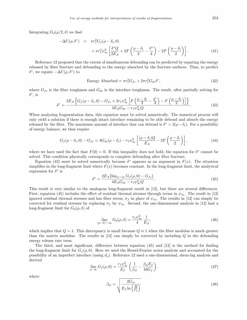
There are very few reports of measured debond lengths during fragmentation that can be used to test thedebonding model. Wagner et al. [12] gives some partial results; they measured debond length as a function ofapplied strain at low crack density or in the long-fragment limit. We can compare their results to predictionsusing the long-fragment result in equation (45); a fit of Wagner’s data [12] to equation (45) is given in Fig. 8.This fit used ds =∞ and Gdc = 200 J/m2. Their is significant scatter in the data, but the fit can be used toderive an estimate for interfacial toughness. The Gdc value here is slightly lower than the Gdc = 264 J/m2

result in [12]. This discrepancy is caused by the different expressions used to find δ∗. Both of these valuesare reasonable toughness values for an interface between glass fibers and a polymer matrix.

6. DISCUSSION

The goal of this paper was to investigate the use of fracture mechanics or energy methods for analyzingfragmentation experiments. All energy methods rely first on deriving an accurate stresses analysis for thefragmentation specimen and second on using that stress analysis to evaluate energy release rates for allrelevant failure mechanisms. Here we considered only fiber fracture and debonding. We needed to calculatethe axial stress in the fiber, the energy release rate for fiber fracture, and the energy release rate for interfacial

0.0 0.2 0.6 0.8 1.0 1.2 1.40.4

Applied Strain (%)

0.0

0.2

0.4

0.6

0.8

1.0

Cra

ck D

ensi

ty (

mm

-1)

50

0

100

250

200

250

300

350

400

Deb

ond

Gro

wth

(fib

. rad

.)

Figure 7. Predicted fragmentation and debond growth results using the fiber strength model with simultaneous debondingcompared to actual experiments. The prediction assumed a perfect interface (ds = ∞), a fiber toughness of Gfc = 10 J/m2,and a debonding toughness of Gdc = 30.5 J/m2. The experimental data is for T50 carbon fibers in an epoxy matrix.


0.0 0.5 1.0 1.5 2.0 2.5

Applied Strain (%)

0

2

4

6

8

10D

ebon

d G

row

th (

fib. r

ad.)

Figure 8. Long-fragment δ∗ as a function of applied strain compared to experimental data. The fit curve used ds = ∞ andGdc = 200 J/m2. The data is for E-glass fibers (with diameter 2r1 = 18.4 µm) in a polymer matrix.

debonding. All calculations were done using the Bessel-Fourier series analysis in [7]. In this section, weconsider the accuracy of the required calculations.

First, fiber fracture is predicted to occur when the stress in the middle of a fragment of aspect ratio ρ−δi(the point of highest tensile stress) becomes equal to the strength of the fiber for that length or when

ψ∞(

1 +⟨σ

(p)zz,1(ρ− δi : ζ = 0)

⟩)= σult(ρ− δi). (49)

Thus, predicting fiber fracture involves accurately determining the average perturbation axial stress in themiddle of the fiber fragment. Now, recall that the Bessel-Fourier series method is an exact elasticity solutionexcept for the axial stress end condition on the fiber. By Saint-Venant’s principle, the stress solution isexpected to be exact except for regions near the fiber break. Because 〈σ(p)

zz,1(ρ− δi : ζ = 0)〉 is evaluated asfar away from the break as possible, it is expected to be very accurate.

Calculating the amount of energy released by a fracturing fiber, Gf (ρ − δi, 0), is a much harder prob-lem. The solution is equivalent to solving the fracture mechanics problem for a penny-shaped crack in aheterogeneous structure — a problem which has not yet been solved. In an attempt to judge the accuracyfor Gf (ρ − δi, 0), we compared it to finite element analysis (FEA) calculations. The comparison, shown inFig. 9, shows that the Bessel-Fourier result agrees with FEA results at high crack density, but is a factor oftwo higher than the FEA results at low crack density. The low crack density results are important becausethey include the long-fragment limit result for Gf (ρ, 0). Unfortunately, it is not certain whether or not theFEA results are correct. The FEA calculation involves selecting a mesh around a crack tip at a bimaterialinterface with two materials that differ significantly in their mechanical problems. The FEA results are meshdependent; i.e., they are not converged. As we continued to refine the mesh within the limits of computermemory and implemented crack-tip elements, the FEA result for Gf (ρ, 0) continued to increase. We suggestthat the correct result for Gf (ρ, 0) lies between the Bessel-Fourier analysis and the FEA calculations.

Accurately calculating Gf (ρ, δi) remains an important problem for using energy methods to analyzefragmentation experiments. We have recently tried to refine the Bessel-Fourier series analysis [19]. In brief,


0 1 3 4 5 6 82

Crack Density (mm-1)

70.0

0.1

0.2

0.6

0.7

0.9

Gf(ρ

,0)

(mJ/

m2 )

0.3

0.4

0.5

0.8 Bessel-Fourier Analysis

Refined Bessel-Fourier Analysis

FEA

Figure 9. Gf (ρ, 0) as a function of crack density using the Bessel-Fourier series analysis, an FEA analysis, or a refinedBessel-Fourier analysis. The plot is for isotropic glass fibers in a polymer matrix with a perfect interface (ds = ∞) usingψ∞ = 1.

we can add more terms to the fiber stress function that are consistent with all boundary conditions, butcontribute non-zero axial stress on the fiber break surface. These extra terms allow us to compensate for theerrors in the fiber end stress inherent in the initial Bessel-Fourier series [7]. With enough extra terms, theaxial stress on the fiber break can be made arbitrarily close to zero (or −1 in the perturbation stresses). Intheory, the refined calculation can therefore be made arbitrary close to the exact result. Figure 9 includesa plot of Gf (ρ, 0) calculated using the refined Bessel-Fourier series analysis [19]. The results fall betweenthe initial Bessel-Fourier analysis and the FEA results, but are still 50% higher than the FEA results atlow crack density. We are currently exploring alternative techniques that can resolve the question about thecorrect result for fiber fracture energy release rate.

We used an very simple analysis to find the energy release rate for debonding, Gd(ρ, δ), for the case ofa frictionless interface. Despite its simplicity, Gd(ρ, δ) is expected to very accurate except for very shortdebond lengths (δ less than a few fiber diameters). The concern about Gd(ρ, δ) is not its accuracy, but theeffect of friction which is expected to present in real experiments. In the presence of friction, the interfacewill slip less than when it is frictionless. The consequence of less slippage is that Gd(ρ, δ) will be lower. Thelowering effect will depend on the coefficient of friction.

When analyzing fragmentation experiments with simultaneous debonding, the extent of debonding can beestimated without any knowledge of Gd(ρ, δ). Revising the fiber-strength failure model to include a debondzone we can write

ψ∞ =σult(ρ− δi)

1 +⟨σ

(p)zz,1(ρ− δi : ζ = 0)

⟩ . (50)

Given experimental data for ψ∞ (calculated from applied strain and thermal load, T ) and ρ (calculatedfrom crack density), we can solve equation (50) for debond size or δi. In brief, the debond size can be backcalculated from experimental data by looking at the difference between a zero-debonding analysis and theexperimental results. This calculation will be inaccurate at low crack density, where the difference betweenexperiments and zero-debonding predictions are small (see Fig. 5), but it will give a good estimate of δi athigh crack density. The need for Gd(ρ, δ) arises when the goal is to deduce an interfacial toughness fromexperimental debond lengths. The results in Fig. 7 show that a frictionless analysis fits the results welland gives us one estimate of Gdc. Because there is no room for improvement, adding the effect of friction


cannot improve the model. What adding friction will do, however, is change the value of Gdc required tofit experimental results. As the coefficient of friction increases, the apparent value of Gdc will also increase.In summary, it will be a useful exercise to include friction in the analysis for Gd(ρ, δ). An accurate frictionanalysis, however, will provide no benefit in interpreting fragmentation results unless there are independentexperimental results that provide the coefficient of friction.

A complete set of fragmentation experiments includes the fiber break or crack density as a function ofapplied strain. Modeling such experiments using energy methods requires input of fiber strength properties,the stress-transfer properties of the intact interface, ds, the fiber toughness, the interfacial toughness, andthe coefficient of friction for the interface. It appears impossible to deduce all require input properties byanalysis of fragmentation results alone. Thus, fragmentation experiments should always be supplementedby other experiments. Fiber strength properties can be measured by experiments on isolated fibers. Theinterfacial stress-transfer properties can be measured using Raman spectroscopy [7, 18]. We need to developmethods for measuring the coefficient of friction. Given these input material properties, the fragmentationtest provides the potential for measuring interfacial toughness, Gdc. Before a deduced Gdc can be claimedto be an interfacial toughness, the model predictions must be compared to observations of debond sizes. Ifthis comparison reveals errors, then the analysis will need to be modified to account for the actual failuremechanisms. Many other possible failure mechanisms will be amenable to the energy methods outlined inthis paper.

Acknowledgements

This work was supported, in part, by a grant from the Mechanics of Materials program at NSF (CMS-9401772), and, in part, by a grant from the United States-Israel Binational Science Foundation (BSF GrantNo. 92-00170), Jerusalem, Israel.

REFERENCES

1. N. J. Wadsworth and I. Spilling, Br. J. Appl. Phys. (J. Phys. D.), 1, 1049–1058 (1968).

2. A. A. Fraser, F. H. Ancker and A. T. DiBenedetto, in: Proc. 30th Conf. SPI Reinforced Plastics Div., Section 22-A,pp. 1–13 (1975).

3. L. T. Drzal, M. J. Rich and P. F. Lloyd, J. Adhesion, 16, 1–30 (1983).

4. W. D. Bascom and R. M.Jensen, J. Adhesion, 19, 219–239 (1986).

5. W. D. Bascom, K-J. Yon, R. M. Jensen and L. Cordner, J. Adhesion, 34, 79–98 (1991).

6. H. D. Wagner, H. E. Gallis and E. Wiesel, J. Mat. Sci., 28, 2238–2244 (1993).

7. J. A. Nairn and Y. C. Liu, Int. J. Solids Structures, 34, 1255–1281 (1997).

8. Z. Hashin, Mech. of Materials, 8, 333–348 (1990).

9. Z. Hashin, in: Inelastic Deformation of Composite Materials, G. J. Dvorak (Ed.), Springer-Verlag, New York, pp. 3–34(1990).

10. P. Feillard, G. Desarmot and J. P. Favre, Comp. Sci. Technol., 49, 109–114 (1993).

11. P. Feillard, G. Desarmot and J. P. Favre, Comp. Sci. Technol., 50, 265–279 (1994).

12. H. D. Wagner, J. A. Nairn and M. Detassis, Applied Comp. Mater., 2, 107–117 (1995).

13. C. H. Liu and J. A. Nairn, Unpublished Results (1996).

14. J. A. Nairn, S. Hu and J. S. Bark, J. Mat. Sci., 28, 5099–5111 (1993).

15. J. A. Nairn and S. Hu, in: Damage Mechanics of Composite Materials, Ramesh Talreja (Ed.), Elsevier, Amsterdam,pp. 187–243 (1994).

16. J. A. Nairn, in: Proc. 10th Int’l Conf. on Comp. Mat., Whistler, British Columbia, Canada, I, pp. 423–430 (1995).

17. Y. Huang and R. J. Young, Comp. Sci. Technol., 52, 505–517 (1994).

18. N. Melanitis, C. Galiotis, P. L. Tetlow and C. K. L. Davies, J. Mat. Sci., 28, 1648–1654 (1993).

19. Y. C. Liu and J. A. Nairn, Unpublished Results (1996).

20. S. G. Lekhnitski, Theory of an Anisotropic Body. MIR Publishers, Moscow (1981).

APPENDIX

In a recent paper [7], the stresses in a fiber fragment in a fragmentation specimen were analyzed using a Bessel-Fourier seriesstress function. The stress analysis satisfies equilibrium and compatibility exactly. It further satisfies all boundary conditions


exactly except for the perturbation axial stress on the fiber end. Instead of the perturbation fiber end stress being exactly -1,only the average perturbation fiber end stress is equal to -1. Substituting the stress function in [7] into the equations in [20] itis possible to find any component of stress, strain, or displacement. Here we quote only those results from [7] that are necessaryfor the calculations in this paper. The required results for a transversely isotropic fiber are⟨

σ(p)zz,1

⟩= B2 +

B3d

2+B3

∞∑i=1

cos kiζ

[c1i

(c

s21− d)I1(β1i)

β1i+ c2i

(c

s22− d)I1(β2i)

β2i

], (A1)

w(p)1 = ζ

(B2

EA− 2νAB1

EA

)+

B3

2GT

[(1− νT )ξ2ζ +

2νAET ρ2

3EAζ

]

+B3

∞∑i=1

sin kiζ

ki

[(−1)i

8νA(1 + νT )

EAk2i

+ c1i

(1

s21GA− d+ 2νAa

EA

)I0(β1ir) (A2)

+ c2i

(1

s22GA− d+ 2νAa

EA

)I0(β2ir)

],

ε(p)zz,1 =

∂w1

∂ζ= −2νAB1

EA+B2

EA+

B3

2GT

[(1− νT )ξ2 +

2νAET ρ2

3EA

]

+B3

∞∑i=1

cos kiζ

[(−1)i

8νA(1 + νT )

EAk2i

+ c1i

(1

s21GA− d+ 2νAa

EA

)I0(β1iξ) (A3)

+ c2i

(1

s22GA− d+ 2νAa

EA

)I0(β2iξ)

],

where

⟨σ

(p)zz,1

⟩is the average fiber stress. The shear stress in the isotropic matrix is

τ(p)rz,2 = B3

∞∑i=1

sin kiζ[c3i (−K1(kiξ)) + c4i

(2(1− νm)K1(kiξ)− kiξK0(kiξ)

)](A4)

Unfortunately, the stresses for an isotropic fiber are not a special case of the anisotropic fiber. The required results for anisotropic fiber are⟨

σ(p)zz,1

⟩= B2 +

B3

2+ 2B3

∞∑i=1

cos kiζ

[c1i

I1(ki)

ki+ c2i

(I0(ki) + 2(1− νf )

I1(ki)

ki

)], (A5)

w(p)1 = ζ

(B2

Ef− 2νfB1

Ef

)+

B3

2Gf

[(1− νf )ξ2ζ +

2νfρ2

3ζ

]+

B3

2Gf

∞∑i=1

sin kiζ

ki

[(−1)i

8νf

k2i

+ c1iI0(kiξ) + c2i(kiξI1(kiξ) + 4(1− νf )I0(kiξ)

)], (A6)

ε(p)zz,1 = −2νfB1

Ef+B2

Ef+

B3

2Gf

[(1− νf )ξ2 +

2νfρ2

3

]+

B3

2Gf

∞∑i=1

cos kiζ

[(−1)i

8νf

k2i

+ c1iI0(kiξ) + c2i(kiξI1(kiξ) + 4(1− νf )I0(kiξ)

)], (A7)

where Ef , Gf , and νf are the Young’s and shear moduli and Poisson’s ratio of the fiber. In the above equations, I0(x) andI1(x) are modified Bessel functions of the first kind, K0(x) and K1(x) are modified Bessel functions of the second kind,

ki =2r1iπ

l=iπ

ρ, and βji =

ki

sj(A8)

where

s21 =a+ c+

√(a+ c)2 − 4d

2d, s22 =

a+ c−√

(a+ c)2 − 4d

2d(A9)


and

a =−νA(1 + νT )

1− ν2AETEA

, b =νT − νAET

EA

(EAGA− νA

)1− ν2

AETEA

,

c =

EAGA− νA(1 + νT )

1− ν2AETEA

, d =

EA2GT

(1− νT )

1− ν2AETEA

.

(A10)

The remaining terms (B1, B2, B3 and cji) are unknowns that must be determined from the boundary and interfaceconditions. For an anisotropic fiber imperfectly bonded to a matrix with an interface parameter, ds, the cji constants are foundby solving a 4× 4 linear system for each term in the Bessel-Fourier series. In matrix form, the linear systems are

(a− 1

s21

)I1(β1i)s1

(a− 1

s22

)I1(β2i)s2(

a− 1s21

)I0(β1i) +

(1−b)s21

I1(β1i)β1i

(a− 1

s22

)I0(β2i) +

(1−b)s22

I1(β2i)β2i

(b−1)

s21

I1(β1i)2GT β1i

(b−1)

s22

I1(β2i)2GT β2i

−(

1s21GA

− d+2νAaEA

)I0(β1i)−

(1s21− a)β1iI1(β1i)

ds−(

1s22GA

− d+2νAaEA

)I0(β2i)−

(1s22− a)β2iI1(β2i)

ds

−K1(ki) 2(1− νm)K1(ki)− kiK0(ki)

K0(ki) +K1(ki)ki

−(1− 2νm)K0(ki) + kiK1(ki)

−K1(ki)2Gmki

−K0(ki)2Gm

K0(ki)2Gm

12Gm

(kiK1(ki)− 4(1− νm)K0(ki)

)

c1i

c2i

c3i

c4i

=

0

(−1)i4(1+νT )

k2i

(−1)i4(1−νT )

2GT k2i

(−1)i8νA(1+νT )

EAk2i

(A11)

Once the cji are known, the remaining constants can be found using

B3 = −

{EA(1− νT )

2

(1− νTET

+ 1 + νmEm

− 2ν2A

EA

)[νAaEA

(1 + νm

Em− 1 + νT

ET

)

− 1

GT

(1− νTET

+1 + νm

Em

)](A12)

+d

2+

∞∑i=1

2(−1)−i[c1i

(c

s21− d)I1(β1i)

β1i+ c2i

(c

s22− d)I1(β2i)

β2i

]}−1

,

B2 =EA(1− νT )

2

(1−νTET

+ 1+νmEm

− 2ν2A

EA

)[νAaEA

(1 + νm

Em− 1 + νT

ET

)− 1

GT

(1− νTET

+1 + νm

Em

)]B3, (A13)

B1 =

νAEA

1− νTET

+ 1 + νmEm

B2 +B3

[(1 + νT )ρ2

3+

(1− νT )a

8

1Gm− 1GT

1− νTET

+ 1 + νmEm

]. (A14)


When the fibers are isotropic, the equations for cji are

−I1(ki) −2(1− νf )I1(ki)− kiI0(ki)

−I0(ki) +I1(ki)ki

−(1− 2νf )I0(ki)− kiI1(ki)

− I1(ki)2Gfki

− I0(ki)2Gf

−(I0(ki)2Gf

+kiI1(ki)ds

)−(

12Gf

+2(1−νf )

ds

)kiI1(ki)−

(2(1−νf )

Gf+k2ids

)I0(ki)

−K1(ki) 2(1− νm)K1(ki)− kiK0(ki)

K0(ki) +K1(ki)ki

−(1− 2νm)K0(ki) + kiK1(ki)

−K1(ki)2Gmki

−K0(ki)2Gm

K0(ki)2Gm

12Gm

(kiK1(ki)− 4(1− νm)K0(ki)

)

c1i

c2i

c3i

c4i

=

0

(−1)i4(1+νf )

k2i

(−1)i2(1−νf )

Gfk2i

(−1)i4νfGfk

2i

(A15)

and the remaining constants are given by

B3 = −

{ν2f

(1Gm− 1Gf

)2

((1− 2νf )

Gf+ 1Gm

) − 1

2

+

∞∑i=1

2(−1)−i[c1i

I1(ki)

ki+ c2i

(I0(ki) + 2(1− νf )

I1(ki)

ki

)]}−1

, (A16)

B2 =

ν2f

(1Gm− 1Gf

)2

((1− 2νf )

Gf+ 1Gm

) − 1

B3, (A17)

B1 =

νfEf

1− νfEf

+ 1 + νmEm

B2 +B3

(1 + νf )ρ2

3− νf

8

1Gm− 1Gf

1− νfEf

+ 1 + νmEm

. (A18)

Documents

On the use of energy methods for interpretation of …forestry.oregonstate.edu/cof/wse/faculty/Nairn/papers/...Composite Interfaces, Vol 4, pp. 241{267 (1996) c VSP 1996 Author prepared