Embed Size (px)
Citation preview
On the Use of a Michelson Interferometer to
Determine Indices of Refraction
John Grasel
5/08/2011
Abstract
The index of refraction of helium gas was measured by recording thenumber of fringes traversing the output of a Michelson interferometeras the helium pressure in an optical cell increased. The LabView codewas extended to use a remote clicker to more accurately identify thepressure in the chamber. Using an algorithm to compute the numberof fringes between data points, the index of refraction of helium was de-termined to be 1+(36.01±0.06)×10−6. The relation between pressureand time was determined to correspond closely to that of compressibleisothermal flow. Using the additional pressure data and a new Fouriertransform analysis, more accurate results for the index of refraction ofhelium, 1 + (35.98± 0.05)× 10−6 were determined.
1
Contents
1 Experimental Setup and Theory 3
2 The Index of Refraction of Helium 52.1 Experiment Adjustments . . . . . . . . . . . . . . . . . . . . . 5
2.1.1 LabView Modifications . . . . . . . . . . . . . . . . . . 52.1.2 Python Digital Signal Processing . . . . . . . . . . . . 6
2.2 Data and Results . . . . . . . . . . . . . . . . . . . . . . . . . 8
3 Investigating the Pressurization of the Cell 103.1 Theory of Pressure Drop Along a Pipe . . . . . . . . . . . . . 103.2 Results . . . . . . . . . . . . . . . . . . . . . . . . . . . . . . . 12
4 Fourier Data Analysis 134.1 Pressure Domain Theory . . . . . . . . . . . . . . . . . . . . . 13
4.1.1 Non-Mathematical Overview . . . . . . . . . . . . . . 134.1.2 Mathematical Analysis . . . . . . . . . . . . . . . . . . 154.1.3 Fourier Transforms in Pressure . . . . . . . . . . . . . 154.1.4 Choosing Sinusoidal Fitting or Fourier Transforms . . 17
4.2 Coding the Resampler . . . . . . . . . . . . . . . . . . . . . . 184.3 Helium Results . . . . . . . . . . . . . . . . . . . . . . . . . . 184.4 Air Results . . . . . . . . . . . . . . . . . . . . . . . . . . . . 19
4.4.1 Sinusoidal Fitting for Air . . . . . . . . . . . . . . . . 194.4.2 Fourier Transform Code . . . . . . . . . . . . . . . . . 204.4.3 Fourier Transform Results for Air . . . . . . . . . . . 21
4.5 Fourier Transform Results for Helium . . . . . . . . . . . . . 22
5 Conclusion 22
6 Graphics 246.1 Helium Fringes vs. Pressure . . . . . . . . . . . . . . . . . . . 246.2 Air Pressure vs. Time . . . . . . . . . . . . . . . . . . . . . . 296.3 Helium Pressure vs. Time . . . . . . . . . . . . . . . . . . . . 326.4 Helium Fringes vs. Pressure . . . . . . . . . . . . . . . . . . . 366.5 Air Fringes vs. Pressure . . . . . . . . . . . . . . . . . . . . . 396.6 Fourier Transform of Air . . . . . . . . . . . . . . . . . . . . . 416.7 Fourier Transform of Helium . . . . . . . . . . . . . . . . . . 46
7 Code Appendix 507.1 process.py . . . . . . . . . . . . . . . . . . . . . . . . . . . . . 507.2 smooth.py . . . . . . . . . . . . . . . . . . . . . . . . . . . . . 577.3 pressure resample.py . . . . . . . . . . . . . . . . . . . . . . . 597.4 fourier transform.py . . . . . . . . . . . . . . . . . . . . . . . 61
2
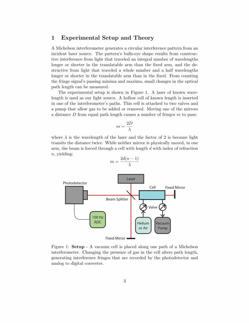
1 Experimental Setup and Theory
A Michelson interferometer generates a circular interference pattern from anincident laser source. The pattern’s bulls-eye shape results from construc-tive interference from light that traveled an integral number of wavelengthslonger or shorter in the translatable arm than the fixed arm, and the de-structive from light that traveled a whole number and a half wavelengthslonger or shorter in the translatable arm than in the fixed. From countingthe fringe signal’s passing minima and maxima, small changes in the opticalpath length can be measured.
The experimental setup is shown in Figure 1. A laser of known wave-length is used as our light source. A hollow cell of known length is insertedin one of the interferometer’s paths. This cell is attached to two valves anda pump that allow gas to be added or removed. Moving one of the mirrorsa distance D from equal path length causes a number of fringes m to pass:
m =2D
λ
where λ is the wavelength of the laser and the factor of 2 is because lighttransits the distance twice. While neither mirror is physically moved, in onearm, the beam is forced through a cell with length d with index of refractionn, yielding:
m =2d(n− 1)
λ
Photodetector
Beam Splitter
Cell
Fixed Mirror
Fixed Mirror
Valve
Heliumor Air
VacuumPump
100 HzADC
Laser
Figure 1: Setup - A vacuum cell is placed along one path of a Michelsoninterferometer. Changing the pressure of gas in the cell alters path length,generating interference fringes that are recorded by the photodetector andanalog to digital converter.
3

To change the index of refraction, we change the pressure. The index ofrefraction n is dependent on pressure P , so the formula becomes
m =2d (n[P ]− 1)
λ
For shorthand, n will be used instead of n[P ]. Values for the index of refrac-tion are quoted at atmospheric pressure P0. The index of refraction minusone is proportional to the pressure, so
n− 1 = αP
P0(1)
where α is the proportionality constant. The index of refraction is definedto be one in a vacuum, where P = 0, which is satisfied by our formula. Theindex of refraction at atmospheric pressure is the quantity of interest:
n[P0]− 1 = α
Substituting our definition of n from Equation (1),
m =αP · 2dλP0
Substituting in α,
m =(n− 1)P · 2d
λP0
Now, all variables are fixed except P and m, so changing one changes theother.
∆m =(n− 1)∆P · 2d
λP0
Rearranging terms,
n− 1 =∆m
∆P
λP0
2d(2)
The objective of the experiment is find the number of fringes m at variouspressures P . A plot of m vs. P has a slope of ∆m/∆P , which by Equation(2) is proportional to the index of refraction. The counting of the fringes isaccomplished by centering the photodiode on the circular fringes and digi-tizing the intensity. Interrupting the laser with an index card at intervalsof equal pressure tags the fringes with marks equally spaced in pressure.For this paper, these intervals of equal pressure are referred to as “isobaricintervals” 1. The fringe intensity sampled at isobaric intervals is referred toas “isobaric data”. Counting the cumulative number of fringes that havepassed from the first isobaric data point to each of the rest yields values form at different P .
1Not to be confused with a system at constant pressure!
4
2 The Index of Refraction of Helium
2.1 Experiment Adjustments
The largest change in the procedure is ensuring that helium is the only gaswithin the chamber. Since its index of refraction (minus one) is one tenththat of air, a small amount of air can tamper with results. The vacuumpump can lower the pressure in the chamber to around 8 mmHg, and thesystem pressure can be safely raised to 800 mmHg. Thus, one ”flush” of thesystem, which consists of evacuating as much of the air as possible and fillingit with helium, removes roughly 1 − 8/800 = 99% of the air, assuming thehelium in the tank is pure. Repeating this process 5 times results in nearlypure helium. In addition, the system was left at a near-vacuum state for tenminutes, and there was no noticeable change in pressure, so leakage is not aconcern.
The given procedure is effective for measuring large indices of refraction,like that of air, but it has some flaws. Firstly, in order to mark the chamberpressure, a mark is made by interrupting the laser beam, but this interruptsvalid data as well. In addition, a human can only determine the position ofan interruption within a fringe period to 1 part in 16. This is insufficientto measure the refractive index of helium. In addition, the computer canuse precise algorithms to determine fractional wavelength, and they havethe advantage of being consistent; i.e, if it consistently overestimates thefractional wavelength, that contributes only to the offset of the m vs. Pgraph, not its slope. Computers can record a click with better resolutionthan an experimentalist can wave an index card, and it requires less efforton the experimentalist. A factor of 10 to 20 more pressure data pointscan be acquired. The computer can process the data rapidly and generateplots to ensure that the algorithm is working properly. These adjustmentsrequire altering the existing LabView code and writing processing softwarein Python.
2.1.1 LabView Modifications
The LabView code was modified to save a list of data points when a key-board or slide advancer key is pressed. Since the sample rate is 100 samplesper second, the time in seconds of any press is equal to its data point indexdivided by 100. The average click is represented by 5-8 samples, correspond-ing to 0.05-0.08 seconds. This is much more responsive than the previousmethod. The clicker used does not register a small fraction of the clicks(roughly 1 in 50), but this is corrected for in the signal processing. It is notknown whether this is a hardware problem in the clicker, an error in thewireless transmission, or a software issue.
5
2.1.2 Python Digital Signal Processing
The processing code was written in Python; the code can be found on Pages50 through 57. After parsing the data files, the average of consecutive presspoints is taken to determine when keys were pressed. An algorithm checks tosee if any clicks appear to be missing, using the fact that the time betweenclicks is roughly linear. If a gap is found, the algorithm will guess the skippedclick occurred halfway between the clicks on either side. This method willfix any single missing point, but will fail when multiple points are skippedin a row.
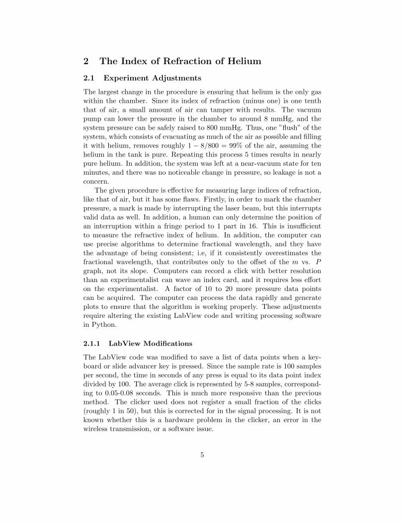
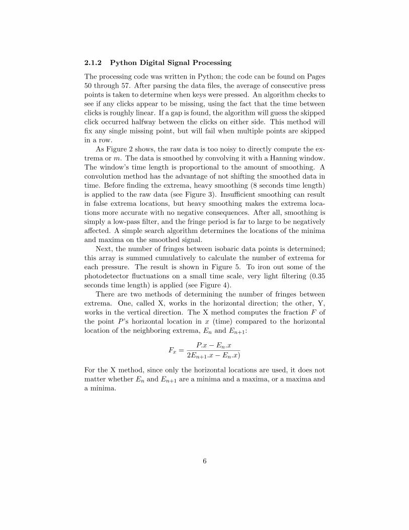
As Figure 2 shows, the raw data is too noisy to directly compute the ex-trema or m. The data is smoothed by convolving it with a Hanning window.The window’s time length is proportional to the amount of smoothing. Aconvolution method has the advantage of not shifting the smoothed data intime. Before finding the extrema, heavy smoothing (8 seconds time length)is applied to the raw data (see Figure 3). Insufficient smoothing can resultin false extrema locations, but heavy smoothing makes the extrema loca-tions more accurate with no negative consequences. After all, smoothing issimply a low-pass filter, and the fringe period is far to large to be negativelyaffected. A simple search algorithm determines the locations of the minimaand maxima on the smoothed signal.
Next, the number of fringes between isobaric data points is determined;this array is summed cumulatively to calculate the number of extrema foreach pressure. The result is shown in Figure 5. To iron out some of thephotodetector fluctuations on a small time scale, very light filtering (0.35seconds time length) is applied (see Figure 4).
There are two methods of determining the number of fringes betweenextrema. One, called X, works in the horizontal direction; the other, Y,works in the vertical direction. The X method computes the fraction F ofthe point P ’s horizontal location in x (time) compared to the horizontallocation of the neighboring extrema, En and En+1:
Fx =P.x− En.x
2En+1.x− En.x)
For the X method, since only the horizontal locations are used, it does notmatter whether En and En+1 are a minima and a maxima, or a maxima anda minima.
6
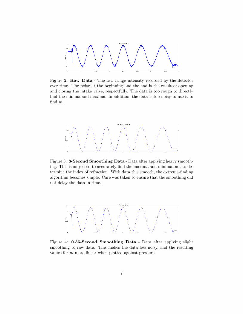
Figure 2: Raw Data - The raw fringe intensity recorded by the detectorover time. The noise at the beginning and the end is the result of openingand closing the intake valve, respectfully. The data is too rough to directlyfind the minima and maxima. In addition, the data is too noisy to use it tofind m.
Figure 3: 8-Second Smoothing Data - Data after applying heavy smooth-ing. This is only used to accurately find the maxima and minima, not to de-termine the index of refraction. With data this smooth, the extrema-findingalgorithm becomes simple. Care was taken to ensure that the smoothing didnot delay the data in time.
Figure 4: 0.35-Second Smoothing Data - Data after applying slightsmoothing to raw data. This makes the data less noisy, and the resultingvalues for m more linear when plotted against pressure.
7

The Y method calculates the horizontal position by using vertical direc-tion y (voltage) with some simple trigonometry:
Fy =1
4± 3
2πarcsin
(2P.y − En.y − En+1.y
2(En+1.y − En.y)
)The plus sign is chosen when En is a minima and En+1 is a maxima, andthe minus sign when the opposite is true.
The X method is inaccurate when the fringe period is changing rapidly,while the Y method is not affected by the fringe period. The Y methoddepends on the maximum intensity being constant over time, and it is lessaccurate near extrema due to the inverse sine function, but the X methoddoes not have these limitations. From experimentation, the Y method worksbest with air, when there are lots of fringes and thus a plethora of verticaldata, and the changing fringe period leaves the X method inaccurate. TheX method works better for helium, though, because there are fewer fringes.Both methods have weaknesses, but the mean difference between the X andY method:
1
N − 1
N−1∑n=1
|Fx − Fy| (3)
is a very conservative estimator of the algorithm’s effectiveness; results showit is 1 part in 30, roughly twice as accurate as a human. While these methodsmay be better than manual estimation, but as they are still non-ideal, thereis still benefit from verifying their effectiveness or circumventing their use.
2.2 Data and Results
The charts of pressure versus fringes are shown in Figures 8, 9, 10, 11, 12,13, 14, and 15. Each chart is the result of five evacuations and fills followed
Figure 5: Final Result - The 0.35-second smoothed data overlayed withidentified extrema (red) and isobaric data points (green). In this case, thefirst and last extrema locations are inaccurate, so X-method calculationswould only be valid between indices 2,000 and 13,500.
8
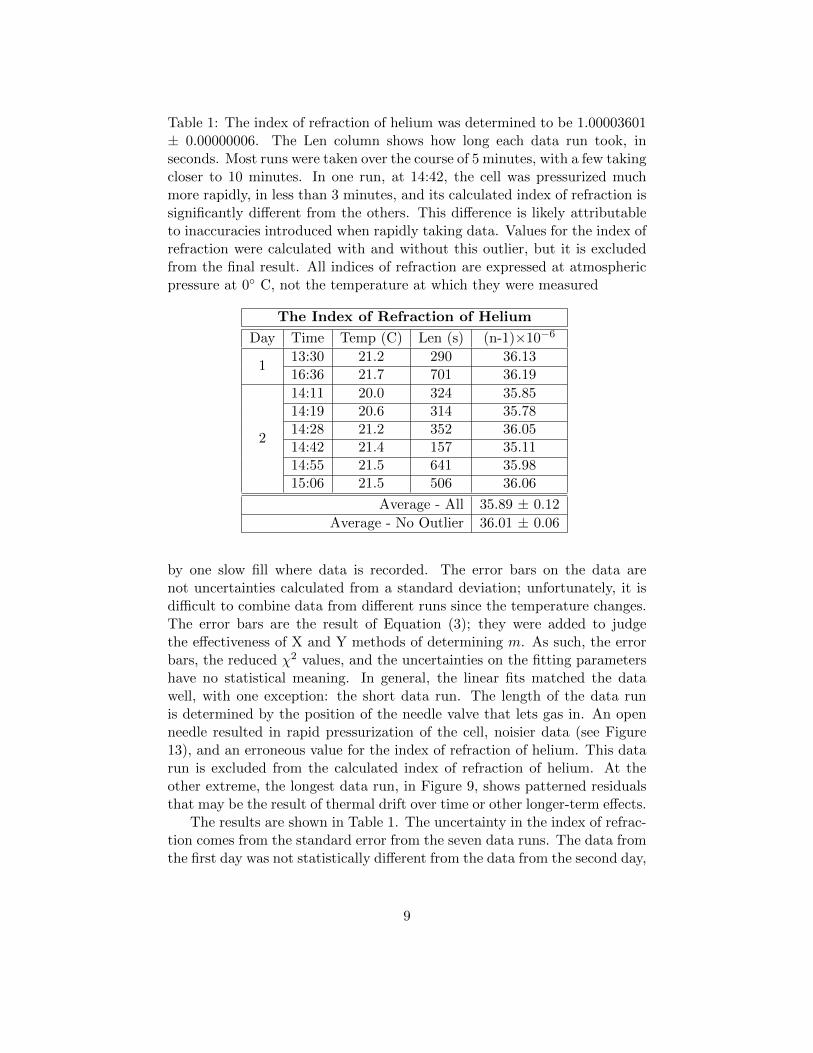
Table 1: The index of refraction of helium was determined to be 1.00003601± 0.00000006. The Len column shows how long each data run took, inseconds. Most runs were taken over the course of 5 minutes, with a few takingcloser to 10 minutes. In one run, at 14:42, the cell was pressurized muchmore rapidly, in less than 3 minutes, and its calculated index of refraction issignificantly different from the others. This difference is likely attributableto inaccuracies introduced when rapidly taking data. Values for the index ofrefraction were calculated with and without this outlier, but it is excludedfrom the final result. All indices of refraction are expressed at atmosphericpressure at 0◦ C, not the temperature at which they were measured
The Index of Refraction of Helium
Day Time Temp (C) Len (s) (n-1)×10−6
113:30 21.2 290 36.1316:36 21.7 701 36.19
2
14:11 20.0 324 35.8514:19 20.6 314 35.7814:28 21.2 352 36.0514:42 21.4 157 35.1114:55 21.5 641 35.9815:06 21.5 506 36.06
Average - All 35.89 ± 0.12
Average - No Outlier 36.01 ± 0.06
by one slow fill where data is recorded. The error bars on the data arenot uncertainties calculated from a standard deviation; unfortunately, it isdifficult to combine data from different runs since the temperature changes.The error bars are the result of Equation (3); they were added to judgethe effectiveness of X and Y methods of determining m. As such, the errorbars, the reduced χ2 values, and the uncertainties on the fitting parametershave no statistical meaning. In general, the linear fits matched the datawell, with one exception: the short data run. The length of the data runis determined by the position of the needle valve that lets gas in. An openneedle resulted in rapid pressurization of the cell, noisier data (see Figure13), and an erroneous value for the index of refraction of helium. This datarun is excluded from the calculated index of refraction of helium. At theother extreme, the longest data run, in Figure 9, shows patterned residualsthat may be the result of thermal drift over time or other longer-term effects.
The results are shown in Table 1. The uncertainty in the index of refrac-tion comes from the standard error from the seven data runs. The data fromthe first day was not statistically different from the data from the second day,
9

so the results were combined. There is certainly no consensus in previousresults, as seen in Figure 6. In fact, there seem to be two distinct camps ofresults, one near 34.75, and the other near 36.0. This new data is the mostprecise value seen, possibly due to the new methods of data analysis and theacquisition of seven data runs instead of the standard five.
3 Investigating the Pressurization of the Cell
Collecting information via computer yielded extra information about thepressure inside of the cell over time. With hundreds of pressure data pointsspaced at intervals of 5 mmHg, it becomes possible to see whether the actualdata matches theory. If so, a curve of best fit of pressure over time canbe computed, which potentially averages out the random error inherent inclicking a button at equal-pressure intervals.
3.1 Theory of Pressure Drop Along a Pipe
Here, an attempt is made to derive the theoretical pressure in the cell overtime. In order to simplify the theory, a few assumptions must be made. Theflow is isothermal because the experiment is not insulated and is exposed tothe ambient environment, and no mechanical work is done on or by the gas.The gas is ideal, which is a good assumption for air at atmospheric pressure,and it is even better for lighter gases like helium and gases at low pressure.The friction factor is constant, and the pipe is straight and horizontal. Then,
Figure 6: There is little consensus within Harvey Mudd regarding the indexof refraction of helium. However, this new data, along with that of two otherstudents, agrees with literature values near 36.
10
the equation for compressible isothermal flow is
w2 =Dρ1A
2
fL
p21 − p2
2
p1
where w is the average mass flow rate, p1 and p2 are the pressures at thebeginning and end of the pipe, ρ1 is the gas density inside the gas reservoir,f is the friction factor, L is the pipe length, D is the pipe diameter, and Ais the cross-sectional area2. By the ideal gas law,
PV = nRT =⇒ dP
dt∝ dn
dt
and the mass flow rate w divided by the molecular mass m is the moleculeflow rate, or
w
m= n =⇒ dw
dt∝ dn
dt
Combining constants,
w2 ∝ p21 − p2
2
p1=⇒ w ∝
√p2
1 − p22
p1
so
dP
dt∝
√p2
1 − p22
p1
giving us our differential equation, with P0 as the outside pressure and P asthe cell pressure,
dP
dt= C1
√P 2
0 − P 2
p1
Solving this differential equation,
P = P0 sin
(C1t+ C2√
P0
)(4)
At first glance, this periodic solution seems nonsensical, since thermodynam-ics states that the system will never move away from equilibrium. However,if the solution is plugged back into the differential equation,
cos
(C1t+ C2√
P0
)=
√cos2
(C1t+ C2√
P0
)2From http://www.pipeflowcalculations.com/pipeflowtheory/pressure-drop-equation-
in-isothermal-flow.php
11

which occurs only whenC1t+ C2√
P0<π
2
Solving for t and plugging that value back into the solution, it is seen thatthe solution only applies when 0 ≤ P ≤ P0. Since this is the region ofinterest, the solution holds.
3.2 Results
The experiment pressure data was fit to the theoretical prediction; firstly,the data taken during the second experiment, when the index of refractionof air was determined, was used. The plots for air data are shown in Figures16, 17, 18, 19, and 20. For all but one graph, the model is a very goodfit. The pressure data does not have associated uncertainty, since each datapoint is a single measurement, so the reduced χ2 values are meaningless,but the residuals are small, and a value of P0 = 750 mmHg is obtained,which is close to atmospheric pressure. Every plot has identically-patternedresiduals, but there aren’t enough data points to draw serious conclusions.
Fortunately, the helium pressure data has an order of magnitude morepoints than its air counterpart. The plots are shown in Figures 21, 22, 23,24, 25, and 26. The data fits the data incredibly well, with residuals under5 mmHg in nearly all cases; this is even more impressive because over ahundred data points were taken, and the pressure dial’s tick resolution is5 mmHg. One oddity is that the calculated P0 is around 900 mmHg, buttheoretically it should be around 1250 mmHg3. This could be a result of thefit not working as well at high pressures, or perhaps there is an issue withthe helium regulator.
The most interesting feature of all but one of these graphs is they sharethe same patterned residuals as the air graphs. The residual pattern lookslike 80% of a sinusoid. The fact that it is present on nearly every graph sug-gests that there is either an issue with the model, or there is an issue withthe experiment. There were no blatant assumptions in the model, and thedata conforms so well to the fit, that it is unlikely that there is an issue withthe model. The residuals are so similar that they’re unlikely to be caused bythermal fluctuations. After examining several causes, it has been hypothe-sized that the residuals are an artifact of a tall experimenter looking down onthe setup, an effect dubbed “perspective error”. At low pressure, when theneedle is facing southwest, a tall experimenter reads a slightly lower valuethan is actually there. The effect reverses at medium pressure, about 400mmHg, where the needle is vertical. The needle continues clockwise untilit’s vertically down near 800 mmHg. The geometry of the setup suggests
31250 mmHg ≈ 1 atmosphere + 10 psi
12
that an experimentalist’s constant head position looking at a needle spin-ning around a dial would yield residual errors that were sinusoidal and of amagnitude comparable to what is seen in the results. The final mystery iswhy Figure 24 on Page 34 has completely flat residuals; this was the datapoint excluded from the value of the index of refraction of helium becausethe data was taken so quickly. It’s possible that the needle was spinning sorapidly, the experimenter leaned in close to see when it was passing pressurepoints, which could eliminate the perspective error. Additional testing isnecessary to verify this hypothesis.
4 Fourier Data Analysis
It has been demonstrated that there is a way to accurately find pressureover time from experimental data. This data can be used to obtain moreaccurate values for the index of refraction of air.
4.1 Pressure Domain Theory
4.1.1 Non-Mathematical Overview
Figure 7 visualizes the non-mathematical concepts of the old method, whichwill hereafter be referenced as time-domain analysis, and the new tech-nique, which is called pressure-domain analysis. Recall that the time-domainmethod involved marking a small number (around 150, ∆P = 5 mmHg) ofequally-spaced-in-pressure points using an automated clicker, or worse, in-terrupting the laser beam to take an even smaller number (around 15, ∆P =50 mmHg) points. These points are used to sample the time-domain fringeintensity signal, keeping tens or hundreds of fringe amplitudes out of tensof thousands recorded by the analog to digital converter. The experimentercan manually estimate the fractional position of each point in the fringe,or the computer can do so digitally, but neither procedure is accurate norprecise. Recall that the slope of the number of fringes vs. pressure plotyields a result proportional to the index of refraction of air. There are tworeasons pressure-domain analysis is more effective: doesn’t throw out over99% of the fringe data4, and it avoids the fuzzy procedure of determiningthe number of fringes between isobaric data points outlined in Section 2.1.2on Page 6.
The pressure-domain method uses the equation relating time to pressure(Equation 4 on Page 11) to fit the pressure data over time. This informationis used to sample the fringe intensity linearly in pressure, keeping the hugeamount of fringe intensity data recorded and putting it to use - the frequency
4At best, the sampling keeps hundreds of data points out of tens of thousands
13
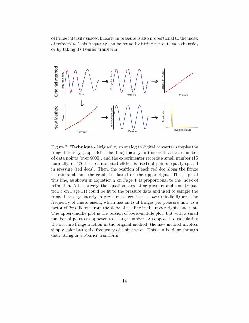
of fringe intensity spaced linearly in pressure is also proportional to the indexof refraction. This frequency can be found by fitting the data to a sinusoid,or by taking its Fourier transform.
Frin
ge A
mpl
itude
Frin
ge A
mpl
itude
Time Pressure Pressure
Num
ber o
f Frin
ges
Tim
e
Pressure Pressure
Frin
ge A
mpl
itude
Am
plitu
de
Inverse Pressure
Orig
inal
Met
hod
New
Met
hod
Figure 7: Technique - Originally, an analog to digital converter samples thefringe intensity (upper left, blue line) linearly in time with a large numberof data points (over 9000), and the experimenter records a small number (15normally, or 150 if the automated clicker is used) of points equally spacedin pressure (red dots). Then, the position of each red dot along the fringeis estimated, and the result is plotted on the upper right. The slope ofthis line, as shown in Equation 2 on Page 4, is proportional to the index ofrefraction. Alternatively, the equation correlating pressure and time (Equa-tion 4 on Page 11) could be fit to the pressure data and used to sample thefringe intensity linearly in pressure, shown in the lower middle figure. Thefrequency of this sinusoid, which has units of fringes per pressure unit, is afactor of 2π different from the slope of the line in the upper right-hand plot.The upper-middle plot is the version of lower-middle plot, but with a smallnumber of points as opposed to a large number. As opposed to calculatingthe obscure fringe fraction in the original method, the new method involvessimply calculating the frequency of a sine wave. This can be done throughdata fitting or a Fourier transform.
14
4.1.2 Mathematical Analysis
The fringe intensity of a non-ideal Michelson interferometer is given by theequation
I = Imax cos2
(2π
λ(L1 − L2) + φ
)+ Imin
where λ is the laser wavelength, L1 and L2 are the fixed and movable pathlengths, and φ a phase term added because the equal-path length positioncan be anywhere in the fringe. Remember that Equation 1 on Page 4 stated
L1 − L2 = 2 (n− 1) dP
P0
so the intensity relation, now a function of pressure, becomes
I[P ] = Imax cos2
(4πd
λP0(n− 1)P + φ
)+ Imin (5)
If the data is fit to a curve,
I[P ] = Imax cos2 (CP + φ) + Imin
where C is a constant, then the index of refraction can be found:
n− 1 = CP0
4π
λ
d(6)
Note that C is related to the slope ∆m/∆P from the linear fit in the oldmethod by the equation:
C = 2π∆m
∆P(7)
Using a trigonometry identity, cosx2 = (1 + cosx)/2, we can also fit to thecurve
I[P ] = Imaxcos(2CP + 2φ) + 1
2+ Imin (8)
4.1.3 Fourier Transforms in Pressure
Once the fringe intensity is resampled to be equally spaced in pressure, thesinusoid’s period must be found. This can be found with a Fourier transformor by fitting the data to Equations 5 or 8. In order to determine which touse, Fourier transforms in pressure space must be investigated. Any functionf [x] defined for −L < x < L can be written as
f [x] = a0 + 2∞∑n=1
an cos (nx) + 2∞∑n=1
bn sin (nx)
15
where
an =1
L
∫ L
−Lf [x] cos (nx)dx
bn =1
L
∫ L
−Lf [x] sin (nx)dx
If cn is defined as an - bn when n > 0 and c†−n when n < 0, then the seriescan be rewritten as
f [x] = a0 + 2∞∑n=1
an(einx + e−inx
)+bni
(einx − e−inx
)=
∞∑n=1
(an − bn) einx + (an + bn) e−inx
=∞∑
n=−∞cne
inx
(9)
Since I[P ] is also a function, it can be expressed as a Fourier series:
I[P ] =∞∑
n=−∞cne
inP
Let the intensity data have N terms at pressures from Pmin to Pmax, a rangeof Prange = Pmax − Pmin. The data is equally spaced at pressure intervalsof Prange/N . With a finite number of terms N in the pressure data, a closeapproximation is made instead. First it is noted that I can be thought of asa function of pressure, or as “the n’th element of the intensity array” In, so
I
[Pmin +
Prange
Nn
]= In
Thus, the approximations become
Cn ≈N−1∑k=0
Ikeink
I[P ] ≈ 1
N
(N−1)/2∑n=−(N−1)/2
Cne2πinP/Prange
where the 1/N factor in the cns was moved from the Cns to I[P ]. The criticalachievement is that the top equation is simply the discrete Fourier transform
16
of the intensity, which is easily computed! Now, if this is rewritten in theform of Equation (8),
I[P ] =1
N
(C0 + Cnmaxe
2πinmaxP/Prange + C−nmaxe−2πinmaxP/Prange
)(10)
where nmax is the index of the peak intensity in the Fourier spectra. We canrewrite Equation (8) as
I[P ] =
(Imin +
Imax
2
)+
(Imax
4e2iφe2iCP
)+
(Imax
4e−2iφe−2iCP
)Comparing this with Equation (10), the Fourier coefficients are related tophysical parameters:
|Cnmax |N
=Imax
4
C0
N= Imin +
Imax
2
C =πnmax
Prange
Solving the equations for the variables of interest,
Imax = 4|Cnmax |N
(11)
Imin =C0
N− Imax
2=C0 − 2|Cnmax |
N(12)
C =πnmax
Prange(13)
As a recap, taking the Fourier transform of intensity data equally spacedin pressure yields a coefficient vector. The index of the maximum element,nmax and its value Cnmax are found, and from these values, all variables ofinterest can be derived, including C, which is proportional to the index ofrefraction (Equation 6).
4.1.4 Choosing Sinusoidal Fitting or Fourier Transforms
Now, two different ways are available to calculate the value C from intensitydata - sinusoidal fitting, or the Fourier transform. The Fourier transformmethod is limited by the resolution of the peak specified nmax. The peakindex is just the closest integer to the “true” value, so the uncertainty onnmax is 1/2. Thus the uncertainty on C is given by
∆C =π
2Prange(14)
17

The experiment uncertainty can be defined as
Uncertainty =∆(n− 1)
n− 1=
∆C
C=
π2Prange
2π∆m∆P
=1
4Prange∆m∆P
=1
4m
where Equation 7 was used for C. In the last step, multiplying a pressurerange times a slope representing the change in the number of fringes per unitpressure results in the total number of fringes traversed m. Thus, the erroris inversely proportional to the number of fringes! For helium, a maximum of5.5 fringes can be acquired over a safe pressure range, so the uncertainty inthe index of refraction is around 12%, an unacceptably high value. However,for air, a maximum of 45 fringes can be acquired, so the uncertainty is only0.6%, a much more acceptable value.
Fortunately, the Fourier transform’s weakness is the sinusoidal fit’s strength:when there are only a few fringes, a sinusoidal fit can accurately calculatethe frequency; however, when there are many fringes, the fit is unable toadapt to minuscule changes in frequency and amplitude, and these can com-pound until the fit no longer agrees with the data. In summary, for gaseswith refractive indices less than or close to that of helium, sinusoidal fittingshould be used. For gases with indices of refraction greater than or near air’sindex of refraction, Fourier transforms are more effective. For the region ofgases between helium and air, either method will work.
4.2 Coding the Resampler
The algorithm for resampling the data linearly in pressure is relativelystraightforward, and the code is attached in the back on Page 59. As be-fore, presses are bunched and the clicks where reliable data starts and endsare noted. Two functions are defined: P [x], which takes a data point indexand turns it into a pressure, and X[p], which does the inverse. P is usedto determine the pressures where good data starts and ends. The intensitydata, which starts linearly in time, is interpolated linearly. A linear spaceof pressure points is created from the start of the accurate pressure data toits end, and each pressure is applied to X, which returns its correspondingpoint. All of these points sample the interpolating function, creating a newfunction of fringe intensities that is sampled linearly in pressure.
4.3 Helium Results
Table 2 shows the results from fitting fringe amplitude data that’s equallyspaced in pressure to a sinusoid. The graphs are shown in Figures 27, 28, 29,30, 31, and 32. The calculated index of refraction is 35.98± 0.05, calculatedwith the mean and standard error of the six trials. The mean very similar to
18
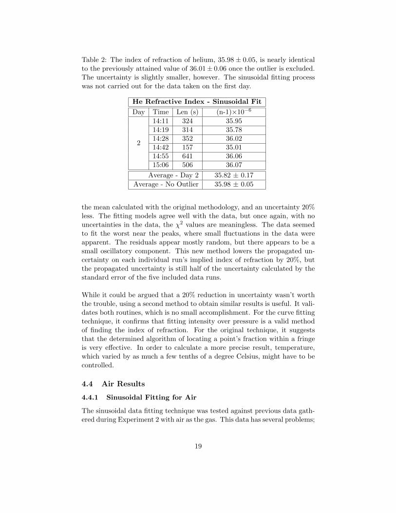
Table 2: The index of refraction of helium, 35.98 ± 0.05, is nearly identicalto the previously attained value of 36.01± 0.06 once the outlier is excluded.The uncertainty is slightly smaller, however. The sinusoidal fitting processwas not carried out for the data taken on the first day.
He Refractive Index - Sinusoidal Fit
Day Time Len (s) (n-1)×10−6
2
14:11 324 35.9514:19 314 35.7814:28 352 36.0214:42 157 35.0114:55 641 36.0615:06 506 36.07
Average - Day 2 35.82 ± 0.17
Average - No Outlier 35.98 ± 0.05
the mean calculated with the original methodology, and an uncertainty 20%less. The fitting models agree well with the data, but once again, with nouncertainties in the data, the χ2 values are meaningless. The data seemedto fit the worst near the peaks, where small fluctuations in the data wereapparent. The residuals appear mostly random, but there appears to be asmall oscillatory component. This new method lowers the propagated un-certainty on each individual run’s implied index of refraction by 20%, butthe propagated uncertainty is still half of the uncertainty calculated by thestandard error of the five included data runs.
While it could be argued that a 20% reduction in uncertainty wasn’t worththe trouble, using a second method to obtain similar results is useful. It vali-dates both routines, which is no small accomplishment. For the curve fittingtechnique, it confirms that fitting intensity over pressure is a valid methodof finding the index of refraction. For the original technique, it suggeststhat the determined algorithm of locating a point’s fraction within a fringeis very effective. In order to calculate a more precise result, temperature,which varied by as much a few tenths of a degree Celsius, might have to becontrolled.
4.4 Air Results
4.4.1 Sinusoidal Fitting for Air
The sinusoidal data fitting technique was tested against previous data gath-ered during Experiment 2 with air as the gas. This data has several problems;
19
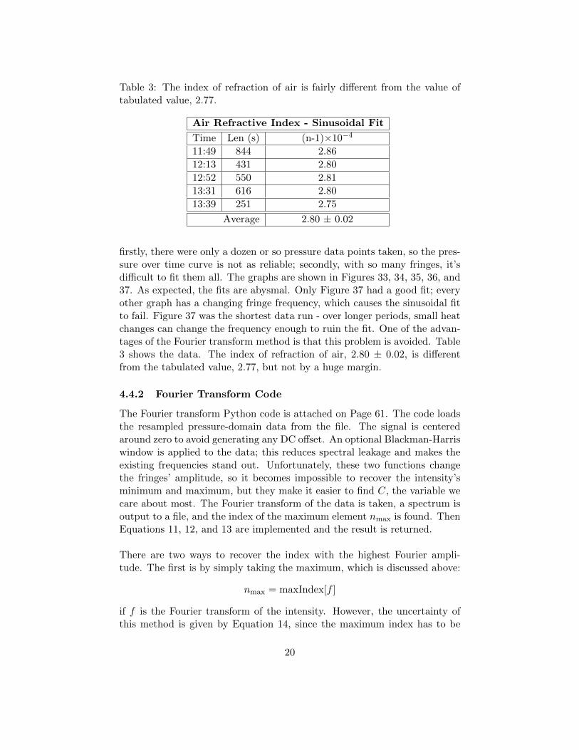
Table 3: The index of refraction of air is fairly different from the value oftabulated value, 2.77.
Air Refractive Index - Sinusoidal Fit
Time Len (s) (n-1)×10−4
11:49 844 2.86
12:13 431 2.80
12:52 550 2.81
13:31 616 2.80
13:39 251 2.75
Average 2.80 ± 0.02
firstly, there were only a dozen or so pressure data points taken, so the pres-sure over time curve is not as reliable; secondly, with so many fringes, it’sdifficult to fit them all. The graphs are shown in Figures 33, 34, 35, 36, and37. As expected, the fits are abysmal. Only Figure 37 had a good fit; everyother graph has a changing fringe frequency, which causes the sinusoidal fitto fail. Figure 37 was the shortest data run - over longer periods, small heatchanges can change the frequency enough to ruin the fit. One of the advan-tages of the Fourier transform method is that this problem is avoided. Table3 shows the data. The index of refraction of air, 2.80 ± 0.02, is differentfrom the tabulated value, 2.77, but not by a huge margin.
4.4.2 Fourier Transform Code
The Fourier transform Python code is attached on Page 61. The code loadsthe resampled pressure-domain data from the file. The signal is centeredaround zero to avoid generating any DC offset. An optional Blackman-Harriswindow is applied to the data; this reduces spectral leakage and makes theexisting frequencies stand out. Unfortunately, these two functions changethe fringes’ amplitude, so it becomes impossible to recover the intensity’sminimum and maximum, but they make it easier to find C, the variable wecare about most. The Fourier transform of the data is taken, a spectrum isoutput to a file, and the index of the maximum element nmax is found. ThenEquations 11, 12, and 13 are implemented and the result is returned.
There are two ways to recover the index with the highest Fourier ampli-tude. The first is by simply taking the maximum, which is discussed above:
nmax = maxIndex[f ]
if f is the Fourier transform of the intensity. However, the uncertainty ofthis method is given by Equation 14, since the maximum index has to be
20
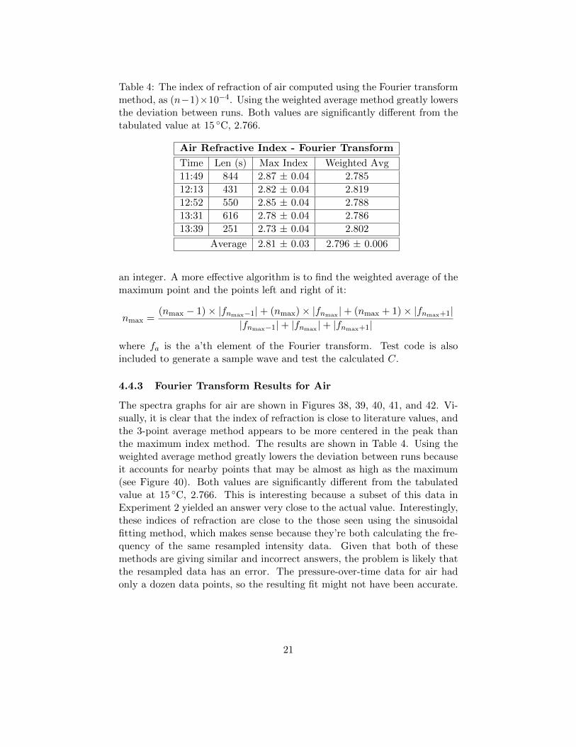
Table 4: The index of refraction of air computed using the Fourier transformmethod, as (n−1)×10−4. Using the weighted average method greatly lowersthe deviation between runs. Both values are significantly different from thetabulated value at 15 ◦C, 2.766.
Air Refractive Index - Fourier Transform
Time Len (s) Max Index Weighted Avg
11:49 844 2.87 ± 0.04 2.785
12:13 431 2.82 ± 0.04 2.819
12:52 550 2.85 ± 0.04 2.788
13:31 616 2.78 ± 0.04 2.786
13:39 251 2.73 ± 0.04 2.802
Average 2.81 ± 0.03 2.796 ± 0.006
an integer. A more effective algorithm is to find the weighted average of themaximum point and the points left and right of it:
nmax =(nmax − 1)× |fnmax−1|+ (nmax)× |fnmax |+ (nmax + 1)× |fnmax+1|
|fnmax−1|+ |fnmax |+ |fnmax+1|
where fa is the a’th element of the Fourier transform. Test code is alsoincluded to generate a sample wave and test the calculated C.
4.4.3 Fourier Transform Results for Air
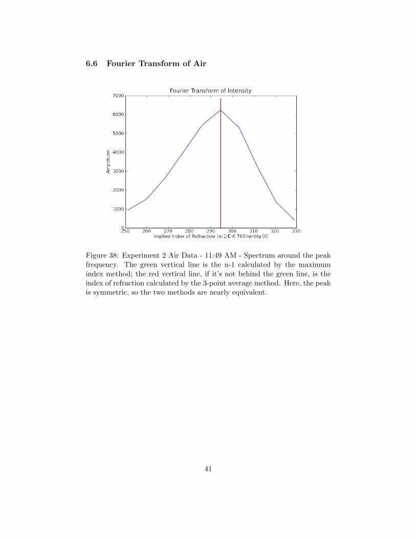
The spectra graphs for air are shown in Figures 38, 39, 40, 41, and 42. Vi-sually, it is clear that the index of refraction is close to literature values, andthe 3-point average method appears to be more centered in the peak thanthe maximum index method. The results are shown in Table 4. Using theweighted average method greatly lowers the deviation between runs becauseit accounts for nearby points that may be almost as high as the maximum(see Figure 40). Both values are significantly different from the tabulatedvalue at 15 ◦C, 2.766. This is interesting because a subset of this data inExperiment 2 yielded an answer very close to the actual value. Interestingly,these indices of refraction are close to the those seen using the sinusoidalfitting method, which makes sense because they’re both calculating the fre-quency of the same resampled intensity data. Given that both of thesemethods are giving similar and incorrect answers, the problem is likely thatthe resampled data has an error. The pressure-over-time data for air hadonly a dozen data points, so the resulting fit might not have been accurate.
21

Table 5: The index of refraction of helium is computed using the Fouriertransform method on Day 2 data, as (n − 1) × 10−6. Using the weightedaverage method greatly lowers the deviation between runs; as expected, themax index uncertainty, which is calculated not as the standard error butpropagated error stemming from the discrete Fourier transform resolution,is too great for results of any significance. However, the weighted averagemethod has a lower uncertainty but gives a different index of refraction fromthe value of 35.98± 0.05 calculated earlier.
Air Refractive Index - Fourier Transform
Time Len (s) Max Index Weighted Avg
14:11 324 33.9 ± 3.4 35.4
14:19 314 34.0 ± 3.4 35.1
14:28 352 34.1 ± 3.4 35.5
14:42 157 33.5 ± 3.4 34.9
14:55 641 33.8 ± 3.4 35.1
15:06 506 34.2 ± 3.4 35.5
Average 34 ± 3 35.24 ± 0.10
4.5 Fourier Transform Results for Helium
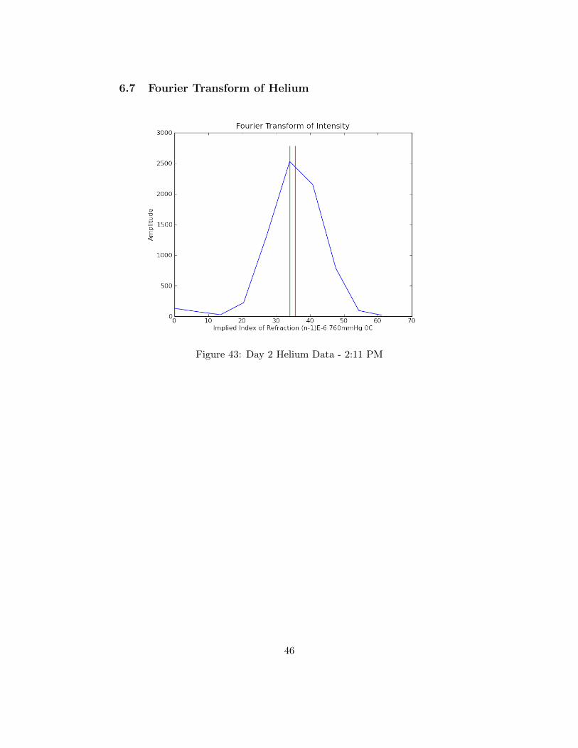
Even though it has already been argued that Fourier analysis is probablynot great for helium, it was trivial to do it after the code had been writtenfor air. The graphs are shown in Figures 43, 44, 45, 46, 47, and 48. The datais shown in Table 5. As expected, the max index uncertainty is too great forresults of any significance. Unlike the weighted average uncertainty, whichis the standard error of the results from individual experiments, the maxindex uncertainty is propagated error stemming from the discrete Fouriertransform resolution (see Equation 14). This is because the uncertaintyfrom the theoretical resolution was greater than the standard error. Sinceboth this Fourier method and the sinusoidal fitting method use the sameresampled pressure data, the resulting values for the index of refractionshould have been closer; however, this can probably be attributed to whathad already been hypothesized: Fourier transform analysis should not beused for gases with indices of refraction as low as that of helium.
5 Conclusion
The LabView modifications and the Python fringe estimator developed inExperiment 2 turned out to be very effective in measuring the index of re-fraction of helium. It also yielded additional pressure and timing data thatopened multiple doors for new methods of data analysis. The pressuriza-
22

tion of the cell over time matched closely to theory, but using that data todetermine the indices of refraction had mixed results, with moderate suc-cess with helium and the sinusoidal fitting, and less success with the Fouriertransform.
23

6 Graphics
6.1 Helium Fringes vs. Pressure
Figure 8: Day 1 1:30 PM - A linear fit is great for this data. Data runconsisted of 5 evacuations and fillings to remove any air from the system,followed by one slow pressurization of the cell while fringe and pressure datawere recorded. The data run was a single measurement without uncertainty,so the error bars shown have no statistical meaning; therefore, the uncer-tainties and the χ2 values are also meaningless.
24
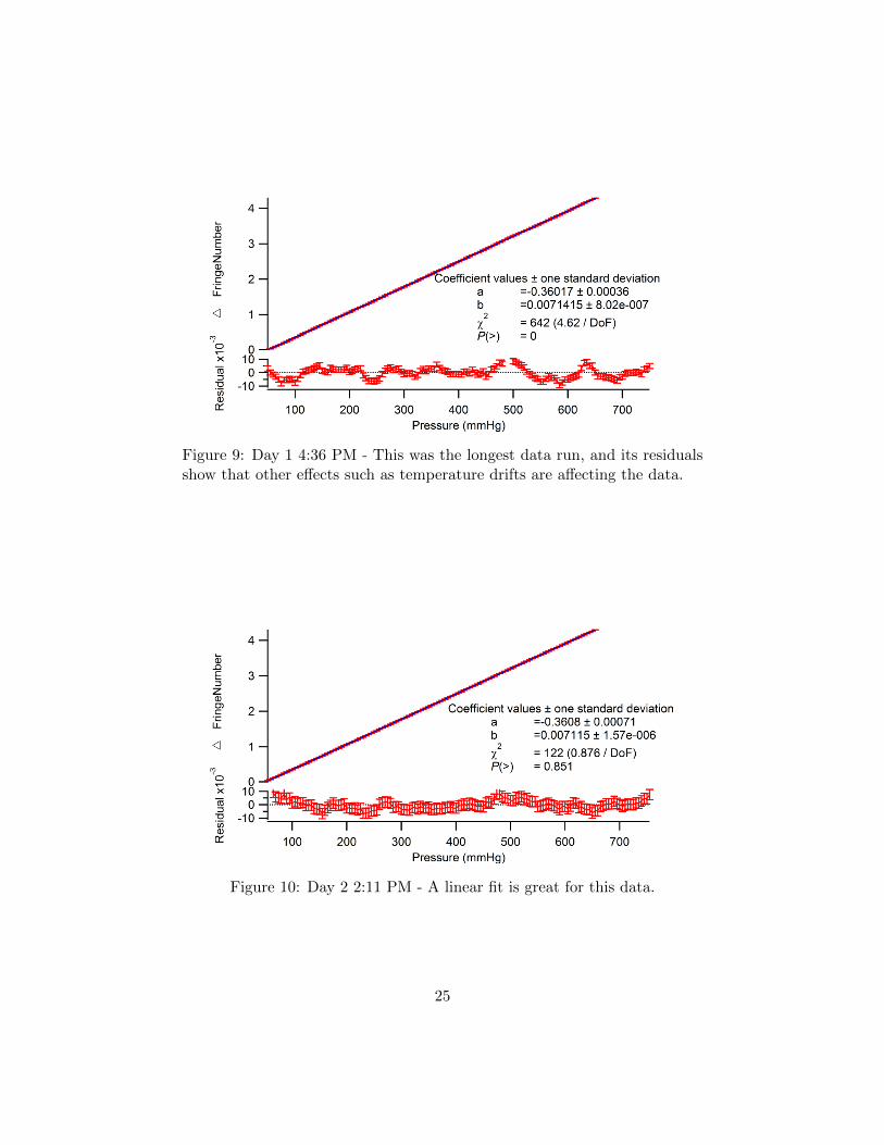
Figure 9: Day 1 4:36 PM - This was the longest data run, and its residualsshow that other effects such as temperature drifts are affecting the data.
Figure 10: Day 2 2:11 PM - A linear fit is great for this data.
25

Figure 11: Day 2 2:19 PM - The first dozen data points do not fit the curvewell, so the data was masked.
Figure 12: Day 2 2:28 PM - A linear fit is good for this data.
26
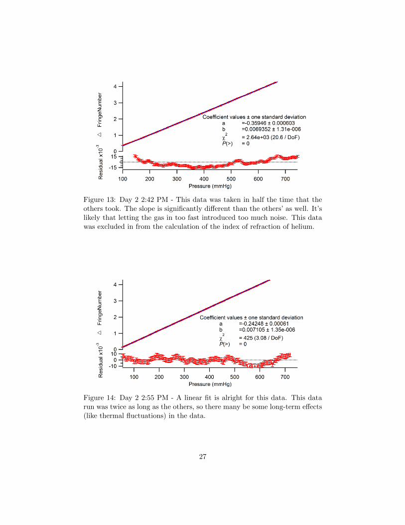
Figure 13: Day 2 2:42 PM - This data was taken in half the time that theothers took. The slope is significantly different than the others’ as well. It’slikely that letting the gas in too fast introduced too much noise. This datawas excluded in from the calculation of the index of refraction of helium.
Figure 14: Day 2 2:55 PM - A linear fit is alright for this data. This datarun was twice as long as the others, so there many be some long-term effects(like thermal fluctuations) in the data.
27

Figure 15: Day 2 3:06 PM - A linear fit is alright for this data, but the errorbars were noticeably smaller for this data set. The error estimator in thePython script isn’t terribly accurate, which is alright since the uncertaintypropagation is not critical here.
28
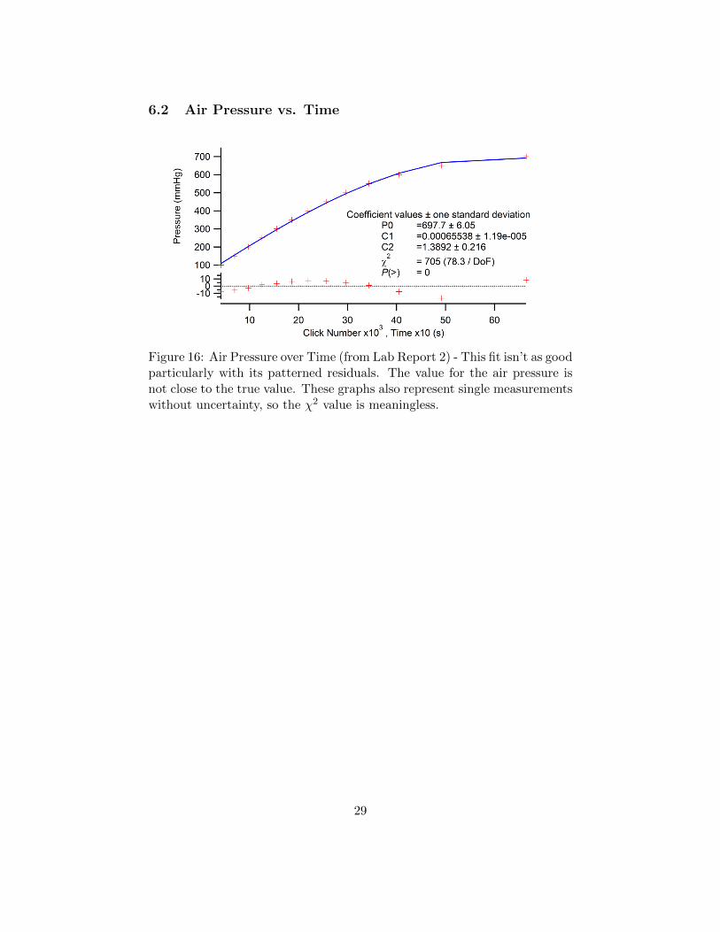
6.2 Air Pressure vs. Time
Figure 16: Air Pressure over Time (from Lab Report 2) - This fit isn’t as goodparticularly with its patterned residuals. The value for the air pressure isnot close to the true value. These graphs also represent single measurementswithout uncertainty, so the χ2 value is meaningless.
29
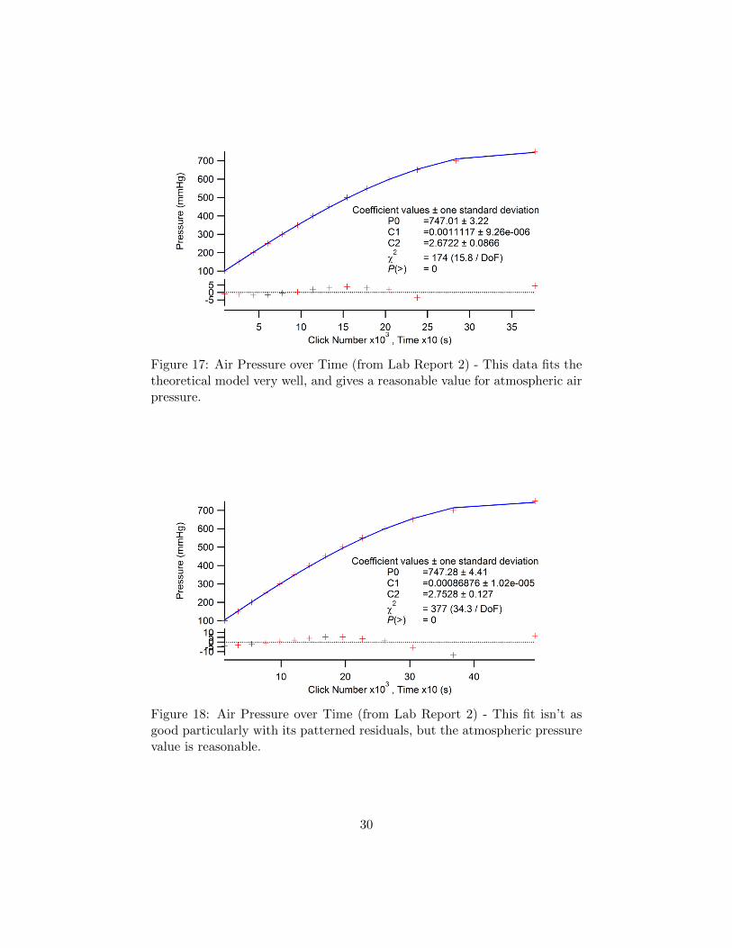
Figure 17: Air Pressure over Time (from Lab Report 2) - This data fits thetheoretical model very well, and gives a reasonable value for atmospheric airpressure.
Figure 18: Air Pressure over Time (from Lab Report 2) - This fit isn’t asgood particularly with its patterned residuals, but the atmospheric pressurevalue is reasonable.
30

Figure 19: Air Pressure over Time (from Lab Report 2) - This fit isn’t asgood particularly with its patterned residuals, and the atmospheric pressurevalue is a little low.
Figure 20: Air Pressure over Time (from Lab Report 2) - This fit is great,as is the atmospheric pressure value.
31

6.3 Helium Pressure vs. Time
Figure 21: Helium Pressure over Time - The data fits the model very well.As before, each data point is a single measurement without uncertainty, sothe propagated uncertainty and χ2 values are meaningless.
32
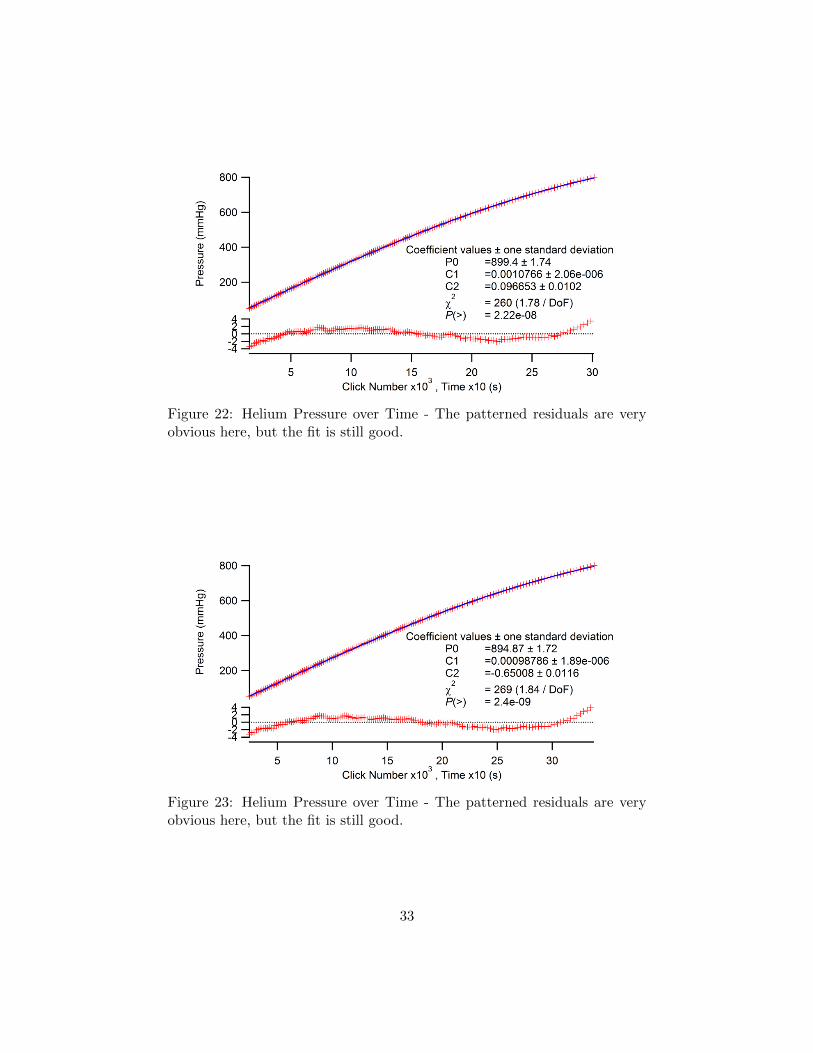
Figure 22: Helium Pressure over Time - The patterned residuals are veryobvious here, but the fit is still good.
Figure 23: Helium Pressure over Time - The patterned residuals are veryobvious here, but the fit is still good.
33
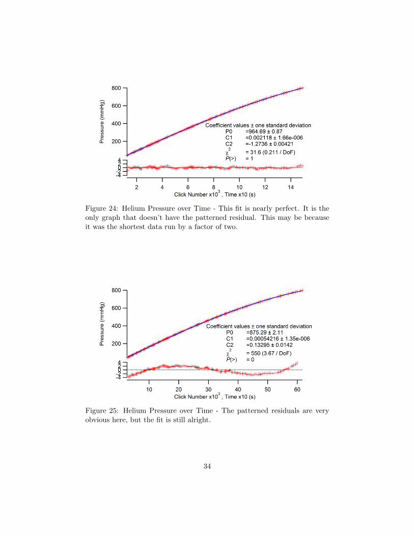
Figure 24: Helium Pressure over Time - This fit is nearly perfect. It is theonly graph that doesn’t have the patterned residual. This may be becauseit was the shortest data run by a factor of two.
Figure 25: Helium Pressure over Time - The patterned residuals are veryobvious here, but the fit is still alright.
34
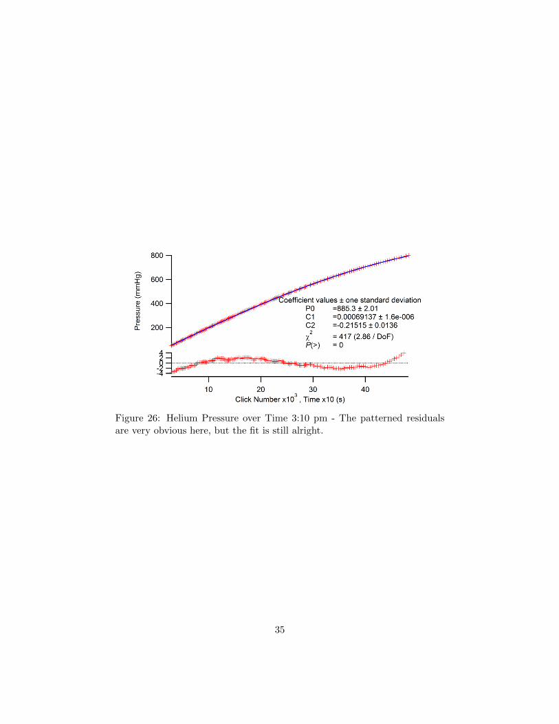
Figure 26: Helium Pressure over Time 3:10 pm - The patterned residualsare very obvious here, but the fit is still alright.
35
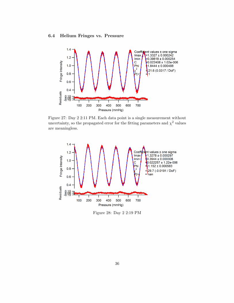
6.4 Helium Fringes vs. Pressure
Figure 27: Day 2 2:11 PM. Each data point is a single measurement withoutuncertainty, so the propagated error for the fitting parameters and χ2 valuesare meaningless.
Figure 28: Day 2 2:19 PM
36
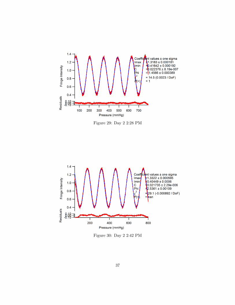
Figure 29: Day 2 2:28 PM
Figure 30: Day 2 2:42 PM
37
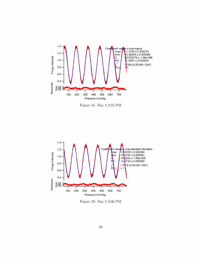
Figure 31: Day 2 2:55 PM
Figure 32: Day 2 3:06 PM
38
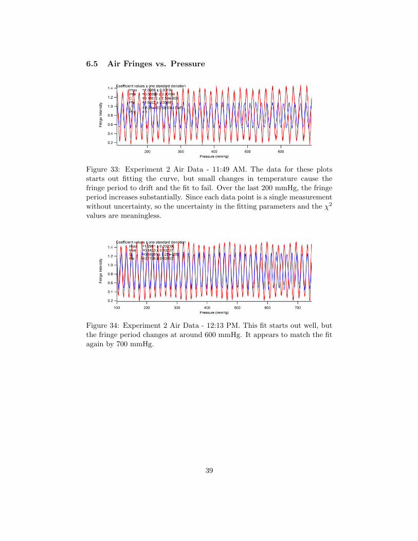
6.5 Air Fringes vs. Pressure
Figure 33: Experiment 2 Air Data - 11:49 AM. The data for these plotsstarts out fitting the curve, but small changes in temperature cause thefringe period to drift and the fit to fail. Over the last 200 mmHg, the fringeperiod increases substantially. Since each data point is a single measurementwithout uncertainty, so the uncertainty in the fitting parameters and the χ2
values are meaningless.
Figure 34: Experiment 2 Air Data - 12:13 PM. This fit starts out well, butthe fringe period changes at around 600 mmHg. It appears to match the fitagain by 700 mmHg.
39
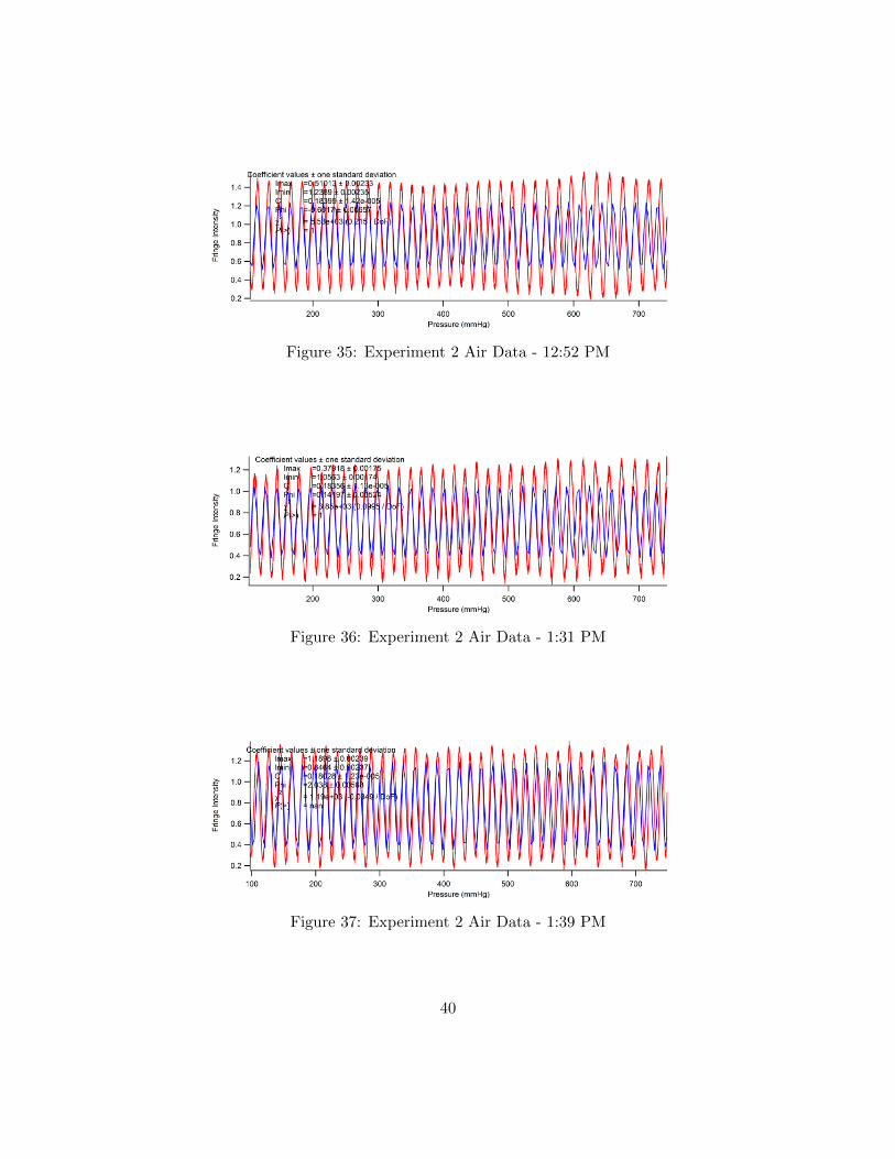
Figure 35: Experiment 2 Air Data - 12:52 PM
Figure 36: Experiment 2 Air Data - 1:31 PM
Figure 37: Experiment 2 Air Data - 1:39 PM
40
6.6 Fourier Transform of Air
Figure 38: Experiment 2 Air Data - 11:49 AM - Spectrum around the peakfrequency. The green vertical line is the n-1 calculated by the maximumindex method; the red vertical line, if it’s not behind the green line, is theindex of refraction calculated by the 3-point average method. Here, the peakis symmetric, so the two methods are nearly equivalent.
41
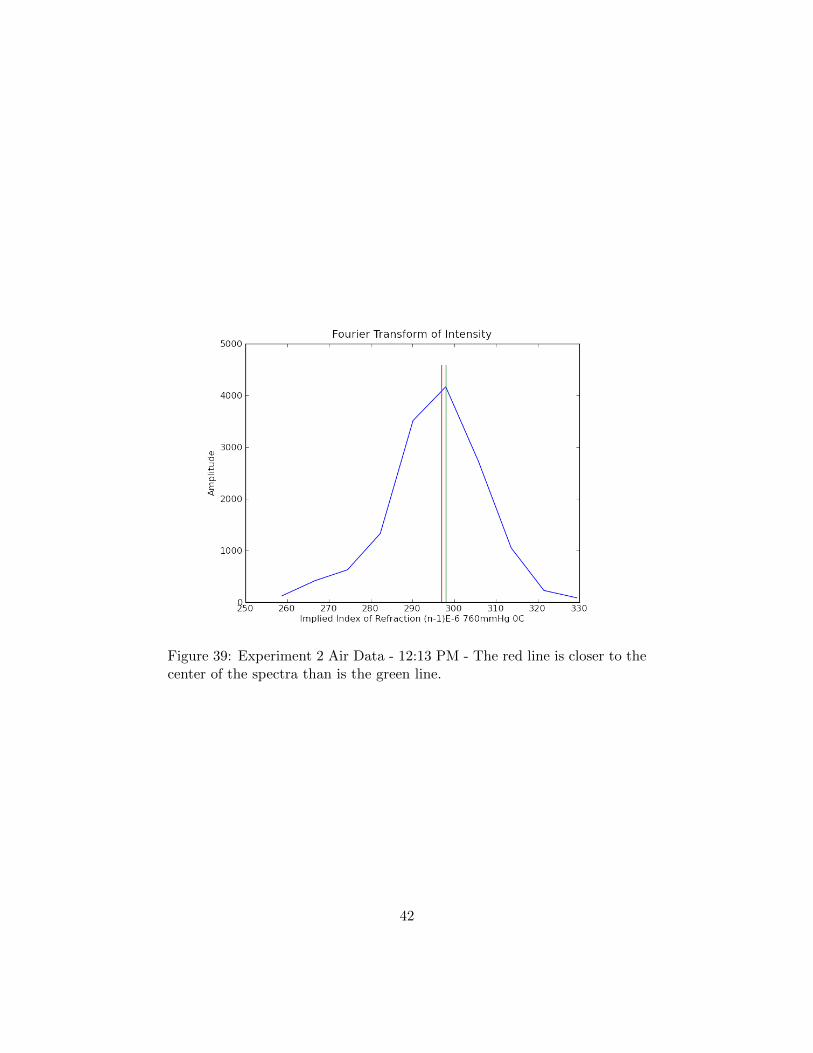
Figure 39: Experiment 2 Air Data - 12:13 PM - The red line is closer to thecenter of the spectra than is the green line.
42

Figure 40: Experiment 2 Air Data - 12:52 PM - When the peaks are ofnearly equal value, the maximum index method (green) is very inaccurate;the average method (red) is closer to the center.
43
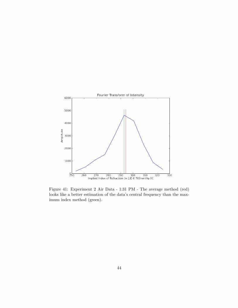
Figure 41: Experiment 2 Air Data - 1:31 PM - The average method (red)looks like a better estimation of the data’s central frequency than the max-imum index method (green).
44
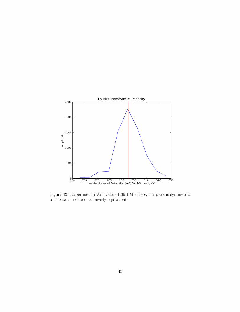
Figure 42: Experiment 2 Air Data - 1:39 PM - Here, the peak is symmetric,so the two methods are nearly equivalent.
45
6.7 Fourier Transform of Helium
Figure 43: Day 2 Helium Data - 2:11 PM
46

Figure 44: Day 2 Helium Data - 2:19 PM
Figure 45: Day 2 Helium Data - 2:28 PM
47
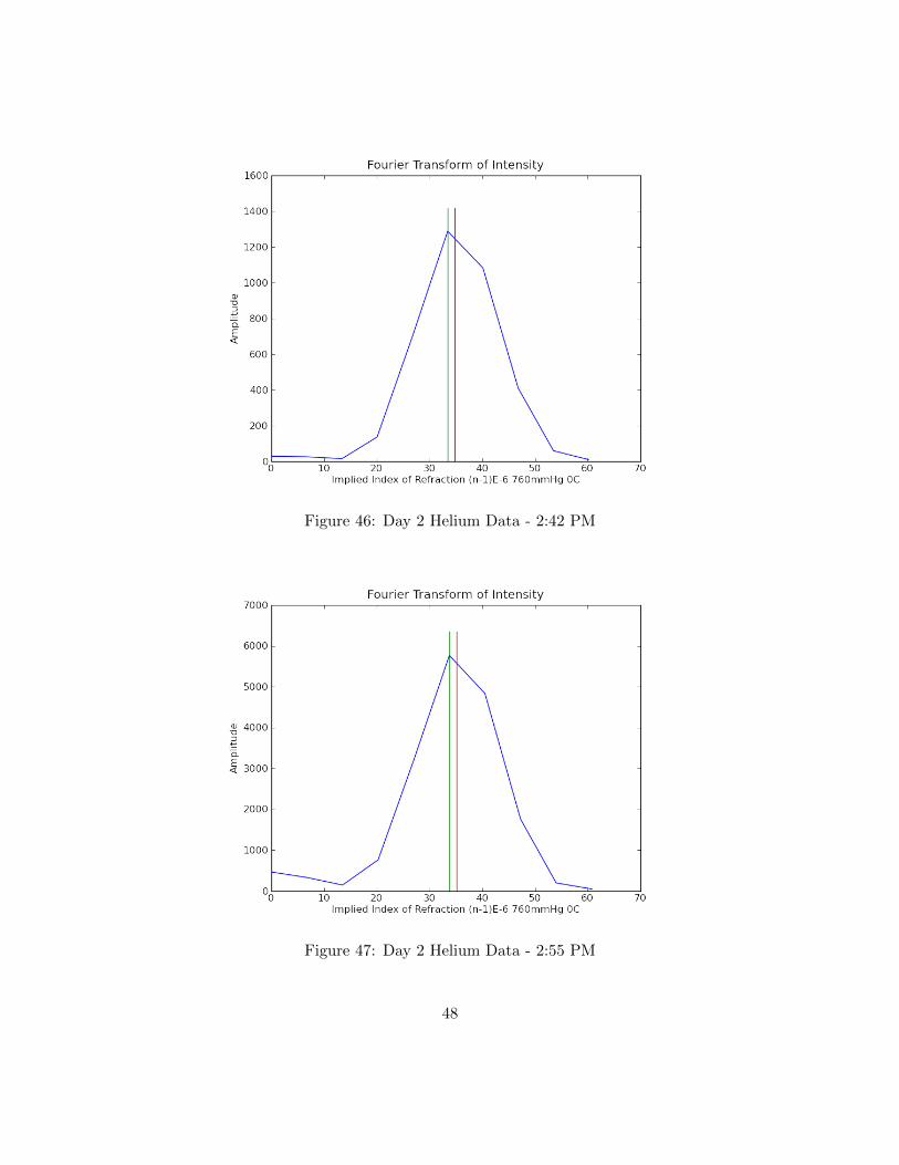
Figure 46: Day 2 Helium Data - 2:42 PM
Figure 47: Day 2 Helium Data - 2:55 PM
48
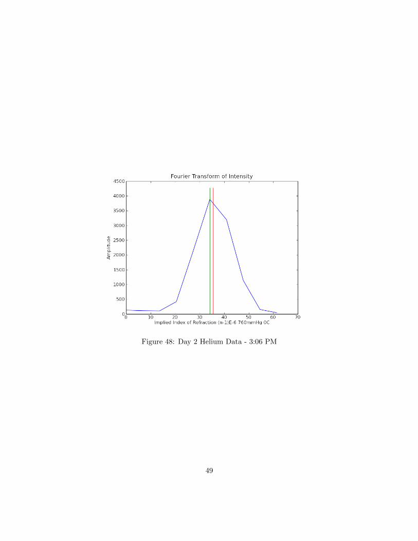
Figure 48: Day 2 Helium Data - 3:06 PM
49

7 Code Appendix
7.1 process.py
1 import os
2 import sys
3 import numpy as np
4 import pylab
5 import math
6
7 import smooth
8
9 crop=2
10
11 def process(data_fstr, press_fstr, debug_dstr,
12 fix_press_errors=True, smooth_presses=True):
13
14 print "Processing %s" % os.path.split(data_fstr)[1].split(’.’)[0]
15 if not os.path.exists(debug_dstr):
16 os.mkdir(debug_dstr)
17
18 # use Numpy to load the data from the text file
19 data, presses = map(np.genfromtxt, [data_fstr, press_fstr])
20
21 # group the key press locations
22 presses = average(group(presses))
23
24 # see if any key presses are missing
25 if fix_press_errors:
26 presses = fix_presses(presses)
27
28 for p in presses:
29 print p
30 print
31 return
32
33 print len(presses)
34 # optionally smooth key press data- USE WITH CAUTION
35 if smooth_presses:
36 presses = buff(presses, crop)
37 print len(presses)
38 savePresses(presses[crop:-crop], os.path.join(debug_dstr, ’presses_raw’), ’Before Smoothing Presses’)
39 spresses = smooth.smooth(np.array(presses), window_len=4)
40 savePresses(spresses[crop:-crop], os.path.join(debug_dstr, ’presses_smooth’), ’After Smoothing Presses’)
41 savePresses((spresses - np.array(presses))[crop:-crop], os.path.join(debug_dstr, ’presses_dif’), ’After Smoothing Presses’)
42 presses = presses[crop:-crop]
43 print len(presses)
44
45 saveArray(data, os.path.join(debug_dstr, ’raw’), ’Before Smoothing’)
46
47 # Calculate the window length with this estimation. Longer data typically has to be
48 # smoothed more! Supersmoothing is used to determine the extrema location. Less
49 # smoothing is necessary for the rest.
50 windowLen = min(800, len(data) / 80)
51 supersmoothdata = list(smooth.smooth(data, window_len=windowLen))
52 saveArray(supersmoothdata, os.path.join(debug_dstr, ’supersmooth’), ’After Super Smoothing’)
53
54 # Normal smooth the data
55 data = list(smooth.smooth(data, window_len=35))
56 saveArray(data, os.path.join(debug_dstr, ’smooth’), ’After Smoothing’)
50
57
58 # Access the voltage where every key was pressed
59 pressHeights = lookup_vals(data, presses)
60
61 # Calculate where the extrema are
62 minmax, firstIsMax = find_extrema(supersmoothdata, int(presses[0]), int(presses[-1]))
63 extremaHeights = lookup_vals(data, minmax)
64 extremas = extrema(minmax, extremaHeights, firstIsMax)
65 plot_extrema_presses(data, minmax, presses, pressHeights,
66 os.path.join(debug_dstr, ’extrema’))
67
68 # Lookup the fractional position of each press between 2 extrema.
69 # f1 does this in X, and f2 does this in Y.
70 f1 = crude_fraction(presses, extremas)
71 f2 = fraction_between_extrema(presses, pressHeights, extremas)
72
73 diff = sum(abs(np.array(f1) - np.array(f2))) / len(f2)
74 print "Average diff between crude & accurate fractions: %.4f wavelengths" % diff
75
76 delta2 = find_deltas(presses, f2, extremas)
77 delta1 = find_deltas(presses, f1, extremas)
78
79 mean2, stdev2 = meanstdev(delta2)
80 mean1, stdev1 = meanstdev(delta1)
81
82 delta2 = [0] + list(np.cumsum(np.array(delta2)))
83 delta1 = [0] + list(np.cumsum(np.array(delta1)))
84
85 for i, x in enumerate(delta2):
86 print i, x, stdev2, delta1[i], stdev1
87
88
89 """ Calculate mean and standard deviation of data x[]:
90 mean = {\sum_i x_i \over n}
91 std = sqrt(\sum_i (x_i - mean)^2 \over n-1)
92 """
93 def meanstdev(x):
94 from math import sqrt
95 n, mean, std = len(x), 0, 0
96 for a in x:
97 mean = mean + a
98 mean = mean / float(n)
99 for a in x:
100 std = std + (a - mean)**2
101 std = sqrt(std / float(n-1))
102 return mean, std
103
104
105 def find_deltas(presses, frac_extremas, extremas):
106 ret = []
107 for i in xrange(len(presses) - 1):
108
109 initial = 0.5 - frac_extremas[i]
110 final = frac_extremas[i+1]
111 extremasIndexAfterInitial = extremas.indexBelowAbove(presses[i])[1]
112 extremasIndexBeforeFinal = extremas.indexBelowAbove(presses[i+1])[0]
113 d = initial + final + (-extremasIndexAfterInitial + extremasIndexBeforeFinal) / 2.0
114 ret.append(d)
115
116 return ret
51
117
118 def crude_fraction(presses, extrema):
119
120 ret = []
121 for X in presses:
122 #print "Press Position: %s" % X
123 lowerExtremaIndex, upperExtremaIndex = extrema.indexBelowAbove(X)
124 Nbefore = extrema.x[lowerExtremaIndex]
125 Nafter = extrema.x[upperExtremaIndex]
126 #print " Extrema Below: #%s @ %s" % (lowerExtremaIndex, Nbefore)
127 #print " Extrema Above: #%s @ %s" % (upperExtremaIndex, Nafter)
128 fraction = (X - Nbefore) / (2.0 * (Nafter - Nbefore))
129 #print " Crude Fraction: %s" % fraction
130 ret.append(fraction)
131
132 return ret
133
134 def fraction_between_extrema(presses, pressHeights, extrema):
135
136 ret = []
137 for X, Y in zip(presses, pressHeights):
138 beforeExtremaIndex, afterExtremaIndex = extrema.indexBelowAbove(X)
139 beforeExtremaYValue = extrema.y[beforeExtremaIndex]
140 beforeExtremaMax = extrema.isMax(beforeExtremaIndex)
141 afterExtremaYValue = extrema.y[afterExtremaIndex]
142
143 if beforeExtremaMax:
144 MIN = beforeExtremaYValue
145 MAX = afterExtremaYValue
146 else:
147 MIN = afterExtremaYValue
148 MAX = beforeExtremaYValue
149
150 X = 0.25 + (3 / (2 * math.pi)) * \
151 math.asin( (2*Y - MIN - MAX) / (2 * (MAX - MIN)))
152
153 if beforeExtremaMax:
154 ret.append(X)
155 else:
156 ret.append(0.5 - X)
157 return ret
158
159
160 def find_extrema(data, start, end):
161 first, firstIsMax = find_extrema_left(data, start)
162 ret = [first]
163 nextIsMin = firstIsMax
164
165 while first < end:
166 first = find_next_extrema(data, first, nextIsMin)
167 ret.append(first)
168 nextIsMin = not nextIsMin
169
170 return ret, firstIsMax
171
172 def find_next_extrema(data, start, isMin, incr = 65):
173 s_0 = start + 2 * incr
174
175 if s_0 > len(data):
176 print "find_next_extrema error: position %i" % start
52

177 s_0 = len(data) - 1
178 raw_input()
179
180 point = data[start]
181 right = data[start + incr]
182 right2= data[s_0]
183
184 if not isMin and point < right and right > right2:
185 return start + index(max, data[start : s_0])
186 if isMin and point > right and right < right2:
187 return start + index(min, data[start : s_0])
188 return find_next_extrema(data, start+incr, isMin, incr)
189
190
191 def find_extrema_left(data, start, incr = 40):
192 s_0 = start - 2 * incr
193 point = data[start]
194 left = data[start - incr]
195 left2= data[s_0]
196
197 if point > left and left < left2:
198 return s_0 + index(min, data[s_0 : start]), False
199 if point < left and left > left2:
200 return s_0 + index(max, data[s_0 : start]), True
201 else:
202 return find_extrema_left(data, start-incr, incr)
203
204
205 def index(function, L):
206 m = function(L)
207 for i, val in enumerate(L):
208 if m == val: return i
209
210
211 def lookup_vals(data, points):
212 return [(1 - p + math.floor(p)) * data[int(math.floor(p))] +
213 ( p - math.floor(p)) * data[int(math.ceil(p))] for p in points]
214
215
216 def average(x):
217 ret = np.empty(len(x))
218 for i in xrange(len(x)):
219 ret[i] = sum(x[i]) / 2.0
220 return ret
221
222 def group(x):
223 ret = []
224 L = len(x)
225 start = None
226 for i in xrange(L):
227 thisEl = x[i]
228 nextEl = x[i + 1] if i+1 < L else None
229 if start is None:
230 start = thisEl
231 if thisEl + 1 != nextEl:
232 end = thisEl
233 ret.append((start, end))
234 start = None
235 return ret
236
53

237 def rename(d, n):
238 return os.path.join(d, n.replace(’.data.txt’, ’.press.txt’))
239
240
241 def savePresses(n, fname, title=’’):
242 xdim = max(len(n) / 600, 8)
243 pylab.figure(figsize = (xdim,6), frameon=False)
244 pylab.plot(n, ’.’)
245 pylab.ylabel(’Press Position’)
246 pylab.xlabel(’Press Number’)
247 pylab.title(title)
248 pylab.savefig(fname + ".png")
249 pylab.close()
250
251
252 def saveArray(n, fname, title=’’):
253 raw_plot(n)
254 pylab.title(title)
255 pylab.savefig(fname + ".png")
256 pylab.close()
257
258 def plot_extrema_presses(data, minmax, presses, pheights, fname):
259 raw_plot(data)
260 for m in minmax:
261 pylab.axvline(x=m, color=’r’)
262
263 pylab.plot(presses, pheights, ’go’)
264
265 pylab.title("Extrema Locations")
266 pylab.savefig(fname + ".png")
267 pylab.close()
268
269 def raw_plot(n):
270 xdim = max(len(n) / 600, 8)
271 pylab.figure(figsize = (xdim,6), frameon=False)
272 pylab.plot(n)
273 pylab.ylabel(’Voltage (V)’)
274 #pylab.ylim([0, 1])
275
276
277 def fix_presses(presses, margin=1.7):
278 """
279 >>> fix_presses([1,2,3,4,5,6,7])
280 [1, 2, 3, 4, 5, 6, 7]
281 >>> fix_presses([1,2,3,5,6,7])
282 Skipped press detected at Point 3
283 Presses are:
284 1 2
285 2 3
286 INSERTING 4.000000
287 3 5
288 [1, 2, 3, 4, 5, 6, 7]
289 >>> fix_presses([1,2,3,5,6,7, 9])
290 Skipped press detected at Point 3
291 Presses are:
292 1 2
293 2 3
294 INSERTING 4.000000
295 3 5
296 Skipped press detected at Point 6
54
297 Presses are:
298 4 6
299 5 7
300 INSERTING 8.000000
301 6 9
302 [1, 2, 3, 4, 5, 6, 7, 8, 9]
303 """
304 new_presses = [presses[0]]
305 lastgap = presses[1] - presses[0]
306
307 for i in xrange(1, len(presses)):
308 newgap = presses[i] - presses[i-1]
309 if newgap > lastgap * margin:
310 newval = (presses[i] + presses[i-1])/2
311 print "Skipped press detected at Point %i" % i
312 print "Presses are:"
313 print i-2, presses[i-2]
314 print i-1, presses[i-1]
315 print "INSERTING %f" % newval
316 print i, presses[i]
317 new_presses.append(newval)
318 newgap /= 2
319 new_presses.append(presses[i])
320 lastgap = newgap
321
322 return new_presses
323
324
325 def buff(L, n=5):
326 """
327 >>> buff([5,6], 1)
328 [4, 5, 6, 7]
329 >>> buff([5,6], 2)
330 [3, 4, 5, 6, 7, 8]
331 >>> buff([5,6, 8], 2)
332 [3, 4, 5, 6, 8, 10, 12]
333 """
334 prv = L[1] - L[0]
335 nxt = L[-1] - L[-2]
336 prv = [L[0] - a * prv for a in reversed(xrange(1, n+1))]
337 nxt = [L[-1] + a * nxt for a in xrange(1, n+1)]
338 return prv + L + nxt
339
340
341 class extrema(object):
342
343 def __init__(self, x_points, y_points, firstIsMax):
344 self.x = x_points
345 self.y = y_points
346 self.firstIsMax = firstIsMax
347
348 def __len__(self):
349 return len(self.x)
350
351 def isMax(self, key):
352 return key % 2 != self.firstIsMax
353
354 def indexBelowAbove(self, x):
355 prevvalue = self.x[0]
356 for index, value in enumerate(self.x[1:]):
55
357 if prevvalue <= x <= value:
358 return index, index+1
359 prevvalue = value
360
361
362 def main(args):
363 join = os.path.join; split = os.path.split
364 this_file = args[0]
365 parent_dir = split(this_file)[0]
366 debug_dir = join(parent_dir, ’debug’)
367 to_process = [x for x in args[1:] if ’.data.txt’ in x]
368
369 if to_process == []:
370 data = join(parent_dir, ’data’)
371 files = [join(data, fn) for fn in os.listdir(data)]
372 main([this_file] + files)
373 else:
374 results = [process(f,
375 join(rename(*split(f))),
376 join(debug_dir, split(f)[1].split(’.’)[0])
377 ) for f in to_process]
378 print results
379
380 if __name__ == ’__main__’:
381 main(sys.argv)
382 raw_input()
56
7.2 smooth.py
1 import numpy
2
3 def smooth(x,window_len=11,window=’hanning’):
4 """smooth the data using a window with requested size.
5
6 This method is based on the convolution of a scaled window with the signal.
7 The signal is prepared by introducing reflected copies of the signal
8 (with the window size) in both ends so that transient parts are minimized
9 in the begining and end part of the output signal.
10
11 input:
12 x: the input signal
13 window_len: the dimension of the smoothing window; should be an odd integer
14 window: the type of window from ’flat’, ’hanning’, ’hamming’, ’bartlett’, ’blackman’
15 flat window will produce a moving average smoothing.
16
17 output:
18 the smoothed signal
19
20 example:
21
22 t=linspace(-2,2,0.1)
23 x=sin(t)+randn(len(t))*0.1
24 y=smooth(x)
25
26 see also:
27
28 numpy.hanning, numpy.hamming, numpy.bartlett, numpy.blackman, numpy.convolve
29 scipy.signal.lfilter
30
31 TODO: the window parameter could be the window itself if an array instead of a string
32 """
33
34 if x.ndim != 1:
35 raise ValueError, "smooth only accepts 1 dimension arrays."
36
37 if x.size < window_len:
38 raise ValueError, "Input vector needs to be bigger than window size."
39
40
41 if window_len<3:
42 return x
43
44
45 if not window in [’flat’, ’hanning’, ’hamming’, ’bartlett’, ’blackman’]:
46 raise ValueError, "Window is on of ’flat’, ’hanning’, ’hamming’, ’bartlett’, ’blackman’"
47
48
49 s=numpy.r_[2*x[0]-x[window_len-1::-1],x,2*x[-1]-x[-1:-window_len:-1]]
50 #print(len(s))
51 if window == ’flat’: #moving average
52 w=numpy.ones(window_len,’d’)
53 else:
54 w=eval(’numpy.’+window+’(window_len)’)
55
56 y=numpy.convolve(w/w.sum(),s,mode=’same’)
57 return y[window_len:-window_len+1]
58
57
59
60
61
62 from numpy import *
63 from pylab import *
64
65 def smooth_demo():
66
67 t=linspace(-4,4,100)
68 x=sin(t)
69 xn=x+randn(len(t))*0.1
70 y=smooth(x)
71
72 ws=31
73
74 subplot(211)
75 plot(ones(ws))
76
77 windows=[’flat’, ’hanning’, ’hamming’, ’bartlett’, ’blackman’]
78
79 hold(True)
80 for w in windows[1:]:
81 eval(’plot(’+w+’(ws) )’)
82
83 axis([0,30,0,1.1])
84
85 legend(windows)
86 title("The smoothing windows")
87 subplot(212)
88 plot(x)
89 plot(xn)
90 for w in windows:
91 plot(smooth(xn,10,w))
92 l=[’original signal’, ’signal with noise’]
93 l.extend(windows)
94
95 legend(l)
96 title("Smoothing a noisy signal")
97 show()
98
99
100 if __name__==’__main__’:
101 smooth_demo()
58
7.3 pressure resample.py
1 import os
2 import sys
3 import numpy as np
4 import process
5 import math
6 import process
7
8 from scipy.interpolate import interp1d
9
10 def resample(data_fstr, press_fstr, fit_fstr, dest_fstr, debug_dstr):
11
12 print "Resampling %s" % os.path.split(data_fstr)[1].split(’.’)[0]
13 if not os.path.exists(debug_dstr):
14 os.mkdir(debug_dstr)
15 if not os.path.exists(fit_fstr):
16 print "Save fit parameters for P0 * Sin((t * C1 + C2]) / Sqrt(P0))"
17 print "Save in %s, in same order as above, one per line" % fit_fstr
18
19 # use Numpy to load the data from the text file
20 data, fit, presses = map(np.genfromtxt, [data_fstr, fit_fstr, press_fstr])
21
22 presses = process.average(process.group(presses))
23 xstart = presses[0]
24 xend = presses[-1]
25
26 @np.vectorize
27 def P(x):
28 return fit[0] * math.sin((x * fit[1] + fit[2]) / math.sqrt(fit[0]))
29
30 @np.vectorize
31 def X(p):
32 return (math.sqrt(fit[0]) * math.asin(p / fit[0]) - fit[2]) / fit[1]
33
34 L = len(data)
35 interpdata = interp1d(range(L), data)
36 print ’.’,
37 pstart = P(xstart)
38 pend = P(xend)
39 pressurePoints = np.linspace(pstart, pend, L)
40 print ’.’,
41 resampled = interpdata(X(pressurePoints))
42 print ’.’,
43 np.savetxt(dest_fstr, np.column_stack((pressurePoints, resampled)))
44 print "Done"
45
46 def rename(f, new):
47 [d, n] = os.path.split(f)
48 return os.path.join(d, n.replace(’.data.txt’, ’.’ + new + ’.txt’))
49
50 def main(args):
51 join = os.path.join; split = os.path.split
52 this_file = args[0]
53 parent_dir = split(this_file)[0]
54 debug_dir = join(parent_dir, ’debug’)
55 to_process = [x for x in args[1:] if ’.data.txt’ in x]
56
57 if to_process == []:
58 data = join(parent_dir, ’data’)
59

59 files = [join(data, fn) for fn in os.listdir(data)]
60 main([this_file] + files)
61 else:
62 [resample(f,
63 rename(f, ’press’),
64 rename(f, ’fit’),
65 rename(f, ’resampled’),
66 join(debug_dir, split(f)[1].split(’.’)[0])
67 ) for f in to_process]
68
69 if __name__ == ’__main__’:
70 main(sys.argv)
60
7.4 fourier transform.py
1 import os
2 import sys
3 import numpy as np
4 import process
5 import math
6 import process
7 import pylab
8 from scipy.interpolate import interp1d
9 from pressure_resample import rename
10 from scipy.signal import get_window
11
12 def fd(data_fstr, img_fstr, debug_fstr):
13 print "Fourier Transforming %s" % os.path.split(data_fstr)[1].split(’.’)[0]
14
15 print data_fstr
16 print img_fstr
17
18 [P, I] = np.loadtxt(data_fstr, unpack=True)[:10]
19 Cnmax, nmax, imax, imin, C, Cerr, C2 = fd_worker(P, I, img_fstr)
20
21 print "Cnmax", Cnmax
22 print "nmax", nmax
23 print "Imax", imax
24 print "Imin", imin
25 print "C %s +/- %s, %s" % (C, Cerr, C2)
26
27 CtoN = 1609.248193
28
29 def fd_worker(P, I, img_fstr):
30 N = len(P)
31 I -= np.mean(I)
32 I *= get_window("blackmanharris", N)
33 f = np.fft.fft(I)
34 nmax = abs(f[:N/2]).argmax(); Cnmax = abs(f[nmax])
35 C0 = abs(f[0])
36 imax = 4 * Cnmax / N
37 imin = (C0 - 2 * Cnmax)/ N
38 C = np.pi * nmax / (P[-1] - P[0])
39 Cerr = np.pi / (P[-1] - P[0])
40
41 Cnmaxm = abs(f[nmax-1])**2
42 Cnmaxp = abs(f[nmax+1])**2
43 Cnmaxs = Cnmax**2
44
45 C2 = ((nmax-1) * Cnmaxm + (nmax) * Cnmaxs + (nmax+1) * Cnmaxp)\
46 / (Cnmaxm + Cnmaxs + Cnmaxp) * np.pi / (P[-1] - P[0])
47
48 x = C / nmax * CtoN * np.arange(max(0, nmax-5), nmax+5)
49 y = abs(f[max(0, nmax-5):nmax+5])
50 pylab.figure(frameon=False)
51 pylab.plot(x, y)
52 pylab.plot([C * CtoN]*2, [0, max(y)*1.1])
53 pylab.plot([C2 * CtoN]*2, [0, max(y)*1.1])
54 pylab.ylabel(’Amplitude’)
55 pylab.xlabel(’Implied Index of Refraction (n-1)E-6 760mmHg 0C’)
56 pylab.title("Fourier Transform of Intensity")
57 pylab.savefig(img_fstr)
58 pylab.close()
61
59
60 return Cnmax, nmax, imax, imin, C, Cerr, C2
61
62
63 def test_fd_worker():
64 C = 0.178
65 Phi = 2.038
66 Imin = 0.34
67 Imax = 1.19
68 DeltaP = .015
69 PStart =50
70 PEnd = 850;
71
72 P = np.arange(PStart, PEnd, DeltaP)
73 I = Imax * (np.cos(2*C*P + Phi) + 1) / 2 + Imin;
74
75 Cnmax, nmax, Imax, Imin, C, Cerr, C2 = fd_worker(P, I, "test.png")
76
77 print "Cnmax", Cnmax
78 print "nmax", nmax
79 print "Imax", Imax
80 print "Imin", Imin
81 print "C %s +/- %s, %s" % (C, Cerr, C2)
82
83
84 def main(args):
85 #if 1:
86 # test_fd_worker()
87 # return
88
89 join = os.path.join; split = os.path.split
90 this_file = args[0]
91 parent_dir = split(this_file)[0]
92 debug_dir = join(parent_dir, ’debug’)
93 img_dir = join(join(parent_dir, "img"), "fd")
94 to_process = [x for x in args[1:] if ’.data.txt’ in x]
95
96 if to_process == []:
97 data = join(parent_dir, ’data’)
98 files = [join(data, fn) for fn in os.listdir(data)]
99 main([this_file] + files)
100 else:
101 [fd(rename(f, ’resampled’),
102 join(img_dir, split(f)[1].split(’.’)[0] + ".png"),
103 join(debug_dir, split(f)[1].split(’.’)[0])
104 ) for f in to_process]
105
106 if __name__ == ’__main__’:
107 main(sys.argv)
62