Embed Size (px)
Citation preview

of the South African Institution of Civil Engineering Volume 58 Number 2 June 2016

1
Contents
of the South African Institution of Civil EngineeringVolume 58 No 2 June 2016 ISSN 1021-2019
PublISherSouth African Institution of Civil EngineeringBlock 19, Thornhill Office Park, Bekker Street, Vorna Valley, Midrand, South AfricaPrivate Bag X200, Halfway House, 1685, South AfricaTel +27 (0)11 805 5947/48, Fax +27 (0)11 805 5971http://[email protected]
edItor-IN-chIefProf Gerhard HeymannUniversity of PretoriaTel +27 (0)12 420 [email protected]
joINt edItor-IN-chIefProf Chris Clayton University of [email protected]
MANAGING edItorVerelene de KokerTel +27 (0)11 805 5947, Cell +27 (0)83 378 [email protected]
jourNAl edItorIAl PANelProf G Heymann – University of PretoriaProf CRI Clayton – University of SouthamptonProf Y Ballim – University of the WitwatersrandProf W Burdzik – University of PretoriaDr P Day – Jones & Wagener (Pty) LtdProf J du Plessis – University of StellenboschProf GC Fanourakis – University of JohannesburgProf M Gohnert – University of the WitwatersrandProf PJ Gräbe – University of PretoriaDr C Herold – Umfula Wempilo ConsultingProf A Ilemobade – University of the WitwatersrandProf SW Jacobsz – University of PretoriaProf EP Kearsley – University of PretoriaProf JV Retief – University of StellenboschProf E Rust – University of PretoriaProf W Steyn – University of PretoriaMr M van Dijk – University of PretoriaProf JE van Zyl – University of Cape TownProf C Venter – University of PretoriaProf A Visser – University of PretoriaDr E Vorster – Aurecon South Africa (Pty) LtdProf J Wium – University of StellenboschProf A Zingoni – University of Cape TownProf M Zuidgeest – University of Cape Town
Peer revIewINGThe Journal of the South African Institution of Civil Engineering is a peer-reviewed journal that is distributed internationally
deSIGN ANd reProductIoNMarketing Support Services, Ashlea Gardens, Pretoria
PrINtINGFishwicks, Pretoria
Papers for consideration should be e-mailed to the Managing Editor at: [email protected]
The South African Institution of Civil Engineering accepts no responsibility for any statement made or opinion expressed in this publication. Consequently, nobody connected with the publication of this journal, in particular the proprietor, the publisher and the editors, will be liable for any loss or damage sustained by any reader as a result of his or her action upon any statement or opinion published in this journal.
© South African Institution of Civil Engineering
Journal of the South African Institution of Civil Engineering • Volume 58 Number 2 June 2016
2 Development of a practical methodology for the analysis of gravity dams using the non-linear finite element methodJ H Durieux, B W J van Rensburg DOI: 10.17159/2309-8775/2016/v58n1a1
14 Shortcomings in the estimation of clay fraction by hydrometerP Stott, E Theron DOI: 10.17159/2309-8775/2016/v58n2a2
25 A qualitative model study on the effect of geosynthetic foundation reinforcement in sand overlying very soft clayB R Jones, S W Jacobsz, J L van Rooy DOI: 10.17159/2309-8775/2016/v58n2a3
35 The effects of under-sleeper pads on sleeper–ballast interactionP J Gräbe, B F Mtshotana, M M Sebati, E Q Thünemann DOI: 10.17159/2309-8775/2016/v58n2a4
42 Stormwater pond efficiency determinations with the effluent probability method: The use of mass versus concentration parametersI C Brink, W Kamish DOI: 10.17159/2309-8775/2016/v58n2a5
49 Stormwater pond metals and solids removal efficiency determination with the effluent probability method: A novel classification systemI C Brink, W Kamish DOI: 10.17159/2309-8775/2016/v58n2a6

2 Durieux JH, Van Rensburg BWJ. Development of a practical methodology for the analysis of gravity dams using the non-linear finite element method. J. S. Afr. Inst. Civ. Eng. 2016;58(2), Art. #708, 12 pages. http://dx.doi.org/10.17159/2309-8775/2016/v58n2a1
techNIcAl PAPerJournal of the South african inStitution of civil engineeringVol 58 No 2, June 2016, Pages 2–13, Paper 708
HAnS DURIEUX (Pr Eng) was enrolled for an MEng in Structural Engineering at the University of Pretoria when this paper was written. He retired at the end of August 2015, but is still active as a private consultant on a freelance basis. He previously worked in the Structural Division in the Directorate Asset Management at the Department of Water and Sanitation
(DWS). He obtained his BSc Eng (Civil) at the University of Pretoria in 1972 and thereafter obtained a BSc Eng (Hons) in 1979 and MEng (Structural Engineering) in 2009. His work experience is in the field of planning and designing of water-related projects at the DWS. Over the last 24 years he has specialised in structural studies of dams, utilising the finite element method.
Contact details: PO Box 40050 Moreleta Park Pretoria 0044 South Africa T: +27 82 809 5302 E: [email protected]
PROF BEn VAn REnSBURG (Pr Eng, FSAICE) is professor in the Department of Civil Engineering in the field of structural engineering. He started his career in consulting engineering and worked in a research organisation, subsequently joining the University of Pretoria. He obtained BSc and MSc degrees in Civil Engineering from the University of Pretoria, an MSc (Structural
Engineering) from the University of Southampton and a PhD (Civil Engineering) from the University of Pretoria.
Contact details: Department of Civil Engineering University of Pretoria Pretoria 0002 South Africa T: +27 12 420 2439 E: [email protected]
Keywords: gravity dams, non-linear finite element method, classical method, singularity point, Drucker-Prager
INtroductIoNThroughout history many methods and theories have been developed to design gravity dams. For many decades the popular ‘classical’ or ‘conventional’ method (CM) was used. This method became virtually a design standard and is still used by many engineers. It is based on the formulation of Bernoulli’s ‘shallow beam theory’. Despite its popularity, the method has many limitations. Its popu-larity can be attributed to its straightforward approach, conservative results and the fact that manual calculations can be done.
The finite element method (FEM) has become a popular tool for analysing complex structures. Although the geometry of a gravity dam is very basic, the structural analysis of such a mass concrete structure is relatively complex, due to the non-linear material behaviour and the variety of static and dynamic loads acting on the structure. In this paper the FEM is investigated as a design tool for analysing gravity dams. Although the FEM is already widely used for this purpose, there are some deficiencies
that have to be addressed in order to fully utilise this method. The major shortcoming of the linear elastic FEM is its sensitivity to mesh density and stress peaks at the points of so-called ‘singularities’. These are posi-tions where the structure has sharp edges, or re-entrant corners, usually leading to infinite stresses. An additional shortcoming of the linear elastic FE analysis is dealing with brittle material behaviour in tension and compression stress zones.
Although in this paper the FEM Drucker-Prager material yield model is illustrated with 2-D models, these principles and con-cepts can also be adapted to 3-D models.
clASSIcAl Method (cM)The theory of the CM is well documented (USBR 1976; CADAM 2001). This method, used to evaluate the stability of a gravity dam, is based on two criteria: (1) the calculation of the tensile stress at the heel and toe of the wall by means of the Bernoulli thin beam formula, and (2) the factor of safety against
development of a practical methodology for the analysis of gravity dams using the non-linear finite element methodJ H Durieux, B W J van Rensburg
For many decades the ‘classical’ method has been used to design gravity dams. This method is based on the Bernoulli shallow beam theory. The finite element method (FEM) has become a powerful tool for the dam design engineer. The FEM can deal with material properties, temperatures and dynamic load conditions, which the classical method cannot analyse. The FEM facilitates the design and optimisation of new dams and the back analysis of existing dams. However, the linear elastic FEM has a limitation in that computed stresses are sensitive to mesh density at ‘singularity points’. Various methods have been proposed to deal with this problem. In this paper the Drucker-Prager non-linear finite element method (DP NL FEM) yield model is presented as a method to overcome the problem of the stress peaks at singularity points, and to produce more realistic stresses at the base of the dam wall. The fundamentals of the DP NL FEM are presented. Benchmark studies of this method demonstrate the method’s viability to deal with zones in a structure with stresses beyond the elastic limit where yielding of the material occurs. A case study of a completed gravity dam is analysed, comparing several analysis techniques. The service and extreme load cases are investigated. Different material properties for the concrete and rock, including weathered material along the base of the wall, are considered. The application and merits of the DP NL FEM are presented. The calculation of the critical factor of safety against sliding is done with a more realistic determination of the conditions along the base of the wall.

Journal of the South African Institution of Civil Engineering • Volume 58 Number 2 June 2016 3
sliding calculated from the Coulomb friction equation. A set of load combinations is evalu-ated according to the design standards. These are based on failure mechanisms relevant to the specific gravity dam. The CM method will not be dealt with in this paper, although the results of a CM analysis with the well-known program CADAM (2001) will be illustrated.
In South Africa and many other countries no official code of practice for dam design is available, and the design criteria, load conditions, acceptable stresses and factors of safety (FOS) are left to the discretion of the approved professional person (APP) and/or design engineers. However, a large variety of SANCOLD (South African National
Committee on Large Dams) and ICOLD (International Commission on Large Dams) publications and guidelines are available to the design engineer.
fINIte eleMeNt Method (feM)The FEM is a powerful design tool for ana-lysing gravity dams, but when the analyses are performed in the linear elastic domain, the problems of stress peaks at the points of singularity have to be addressed. Figure 1 illustrates the singularity problems at the heel and toe of the wall of a gravity dam for a homogeneous wall and foundation. The heel is defined as the position where the upstream face of the wall intersects the foundation face. Similarly the toe is defined as the posi-tion where the downstream face of the wall intersects the foundation face.
The points where singularities emerge are important positions in gravity dam design. In order to address the singularities problem for linear FE analysis, the following solutions were investigated by Durieux (2009):
■ Identify points where singularities occur and disregard the peak stresses within a small restricted area.
■ Use a relatively coarse FEM mesh to eliminate the singularity effects, but still capture the essential stresses in the wall section with reasonable accuracy.
■ Employ ‘stress linearisation’. ■ Modify the geometry to incorporate a fil-
let or round-off radius, relaxing the stress concentration.
Non-linear analysis techniques provide more realistic stress distributions at singularities:
■ Fracture mechanics techniques which simulate crack development at the sin-gularity point and redistribute the stress surges.
■ Contact elements follow a prescribed path and open when a specified tensile stress occurs, and thus relieve tensile stresses.
■ Non-linear material methods, such as the Mohr-Coulomb and Drucker-Prager yield models, which will be the focus of this paper.
Illustration of the singularity effect on a hypothetical triangular dam in 2-dTo illustrate the effect of the singularity problem on a gravity dam, a 2-D plane strain FE model of a hypothetical triangular dam was created with different mesh densities. Mesh densities of 4, 8, 12, 20, 40, 80 and 160 elements along the base of the wall were modelled. Figure 2 illustrates some of these mesh densities for a 100 m high triangular gravity dam with a downstream slope of 1:0.8. A monolithically FEM mesh was used, i.e. wall
Figure 1 Illustration of singularity points where stress peaks occur
Singularity points
ToeHeel
Figure 2 Triangular gravity dam – mesh densities with 4, 8, 20 and 160 elements at the base

Journal of the South African Institution of Civil Engineering • Volume 58 Number 2 June 20164
and foundation were only distinguished by their material properties, but no discontinuities were introduced, such as contact elements.
The load conditions applied are: (a) hydro-static pressure of 100 m water applied on the upstream face, (b) full uplift pressure under the wall (triangular distribution from 1 MPa at the heel to zero at the toe), and (c) self-weight of the concrete wall. The MSC Marc FE program was used (MSC Marc 2003).
The material properties of a typical concrete gravity dam were used, i.e. elastic modulus for concrete Ec = 20 GPa, Poisson’s ratio υ = 0.22 and density ρ = 2 400 kg/m³. For the foundation, Er = 30 GPa and υ = 0.25 were used. No density was incorporated into
the foundation block. The boundary condi-tions were applied on the foundation block and were fixed on the lower circumference in the x and y directions. The last mesh illus-trated in Figure 2 is one-way biased to limit the number of elements, but still has the cor-rect element size at the heel of the wall.
Figure 3 illustrates the contour plot of the vertical normal stress (Sy) for a mesh density of a one-way biased 160 elements at the base of the wall. The load case was for the above-mentioned load condition. The maximum vertical normal stress Sy at the heel of the wall is 5.30 MPa.
Figure 4 illustrates the distribution of normal tensile stress Sy at the heel of the wall
for the seven mesh densities. The load condi-tions (as outlined above) were the same for all the analyses.
The normal stress Sy at the heel of the wall in Figure 4 varies from 0.36 MPa to 5.30 MPa for the 4 to 160 element mesh den-sities, illustrating the large disparity in the stress. The question is, which stress is the correct one to represent the stress condition at the heel of the wall?
The main stability criterion used in the CM is based on calculating the stress at the heel of the wall and assessing it with an allowable tensile stress for a given load condition. However, when the same evalu-ation criterion is used with the linear FEM, conflicting conclusions on the safety of the structure can be reached, due to the large stress variation at the heel depending on the mesh density (illustrated in Figure 4). It is thus necessary to adopt another evaluation criterion for the FEM.
One of the methods mentioned above to address the singularity problem in an FEM is to use the non-linear material yield models. The Drucker-Prager (DP) yield model is well suited to deal with this problem, but then an alternative evaluation criterion would have to be adopted for gravity dams. The authors have found that a useful technique for evalu-ating the structural behaviour of a gravity wall, utilising the non-linear FEM, is by com-puting the equivalent plastic strain (EQPS) of the wall for the given load conditions. The EQPS provides a means of measuring the material yielding in the plastic zone (plastic strain) and presents the areas where plastic material yielding is assumed to occur. The EQPS can be illustrated on a graph present-ing the normal stress versus strain. The position where the EQPS starts is where the curve deviates from the linear relationship (see Figure 5 in next section).
deterMINAtIoN of the PArAMeterS for the drucker-PrAGer Model froM StANdArd lAborAtory teStSThe theory of the DP model is well docu-mented in text books, such as Zienkiewicz (1977) and Chen (1982).
A simplified uni-axial stress-strain curve for the DP ideal plastic model is presented in Figure 5, which illustrates the linear and non-linear relationship between stress and strain.
In Figure 5 the stress-strain curve illus-trates that the theory of the linear plastic DP (also called the ideal plastic DP) is a conser-vative approach, because the linear horizon-tal line of the relationship deviates from the non-linear stress-strain curve when entering
Figure 4 Maximum vertical normal stresses at the heel of the triangular gravity dam for different numbers of elements along the base
Nor
mal
str
ess S
y (M
Pa)
6
5
Sensitivity of mesh density on a triangular gravity dam (100 metres high)
4
3
2
1
0
Number of elements180160140120100806040200
0.360.70
1.00
1.49
2.36
3.57
5.30
SyyL
Figure 3 Vertical normal stresses for a triangular gravity dam with a mesh density of 160 elements along the base
5.30+0004.81+0004.32+0003.83+0003.34+0002.85+0002.36+0001.87+0001.38+0008.85–0013.94–001
–9.66–002–5.87–001–1.08+000–1.57+000–2.06+000
–2.06
MSC Patran 2005 r2 25-Sep-08 13:54:44
Fringe: Default Static Step, A1:Incr=0, Time=0.00000, Stress, Global System, Y Component, At Layer 1
default_Fringe:Max 5.30+000 @ Nd 1Min –2.06+000 @Nd 4521default_Deformation:Max 1.62–002 @ Nd 4638
X
Y

Journal of the South African Institution of Civil Engineering • Volume 58 Number 2 June 2016 5
the non-linear region. This implies that the yielding stress of the material is kept con-stant at a lower stress level below the actual stress-strain relationship. This approach is valid only until the horizontal (dotted) line intersects the non-linear curve. The DP analysis should be kept within this strain region to ensure a conservative approach.
Figure 6, from Zienkiewicz (1977), illus-trates the Mohr-Coulomb, Tresca, Drucker-Prager (DP) and Von Mises material yield criteria. It should be noted that the stresses are illustrated in the negative zones. The envelopes represent the failure domain. σ1, σ2 and σ3 are the maximum, intermediate and minimum principal stresses respectively, φ is the internal friction angle and c the cohesion.
This paper will focus on the Drucker-Prager yield criterion.
basic theory of the drucker-Prager modelIn Chen (1982) and MSC Marc (2003) the following equation of the Drucker-Prager yield criterion is given:
f = αJ1 + J2½ –
σ
√3 = 0 (1)
The equations for calculating the c and φ are given in terms of α and σ:
c = σ
[3(1 – 12α2)]½; Sin φ =
3α
(1 – 3α2)½ (2)
where: c = cohesion of material φ = internal friction angle of material σ = calculated yield stress α = DP constant
J1 (MSC Marc 2003) or I1 (Chen 1982) is the first invariant of the stress tensor:
J1 = σii with σii = σ1+ σ2+ σ3
J2 is the second invariant of the stress tensor:
J2 = 1
2 σij σij
σii and σij are stress tensors
σ1, σ2 , σ3 are maximum, intermedi-ate and minimum principal stresses respectively.
Chen (1982) gives:
f(I1, J2) = αI1 + √J2 – k (3)
where:
k = σ
√3 (4)
Chen (1982) also gives the equations for determining the values of friction and cohe-sion in terms of the tensile and compressive yield strength of the material:
Sin φ = fc – ft
fc + ft and c =
fc ft
fc – ft Tan φ (5)
where: ft = tensile strength of material fc = compressive strength of material
Figure 6 Graphical illustrations of the different yield criteria (Zienkiewicz 1977)
√3c cot φ
–σ3
Mohr-Coulomb φ > 0
σ1 = σ2 = σ3
Tresca φ = 0
–σ2
–σ1
Drucker-Prager φ > 0
–σ3 σ1 = σ2 = σ3
Von Mises φ = 0
–σ2
√3c cot φ
–σ1 (a) (b)
Figure 5 Simplified stress-strain curves for uniaxial material tests used in the Drucker-Prager theory
Stress
DP linear plastic curve
+
+
Non-linear region
Linear regionIdeal plastic region
Tension area
Strain
Linear region
Compressive area
Ideal plastic region
Non-linear region
–
–

Journal of the South African Institution of Civil Engineering • Volume 58 Number 2 June 20166
By substituting these values of φ and c in Equation (2) the parameters for the DP model (σ and α) can be obtained.
From the above equations it can be seen that, by simply using the tensile and compres-sive strengths of the concrete, all the necessary parameters for the DP model can be derived. These material properties can be obtained from standard material laboratory tests.
beNchMArkS APPlyING the drucker-PrAGer ModelTo evaluate the accuracy of the DP non-linear FEM (DP NL FEM) to address the singularity problem in concrete structures, a series of benchmarks were conducted.
The DP NL FEM analyses were computed with MSC Marc (2003) using the non-linear material facility. The loads were divided into time-steps and ramped from zero to maximum value during specific time-steps.
The load time-stepping is necessary to accomplish correct convergence in the FE program for material yielding throughout the structure. For each time-step an iterative process was used to ensure that complete convergence had been obtained. Convergence is defined as a solution of which the results for stress or deformation congregate to a single value through the prescribed time-steps and iterations, and the oscillation of the results stabilises within the given convergence tolerances.
The benchmarks from, amongst others, Bhattacharjee and Léger (1994) and Carpinteri et al (1992) were arranged and conducted, and
described comprehensively in Durieux (2009), according to the level of complexity:
■ Simple tensile specimen ■ 2-D standard beam test ■ 2-D standard shear beam ■ Model gravity dam ■ Full-size concrete gravity dam.
One benchmark of a model gravity dam (as shown in Figure 7), 2.4 m high, of Carpinteri et al (1992) is summarised by way of illustra-tion. This benchmark was chosen because information on the physical laboratory model and the results of a fracture mechanics study by Bhattacharjee and Léger (1994), same FE model as illustrated in Figure 7, were available.
Figure 7 Schematic presentations of the model gravity dam and the EQPS in notch at a force of 750 kN
0.25
0.08
CMOD2.00 0.
152.
40
3.64–004MSC Patran 2005 r2 22-Jan-07 12:13:29
Fringe: Constant, A1:Incr=40, Time=3.00000, Strain, Total Plastic Equivalent (from rate), , (NON-LAYERED)
default_FringeMax 3.64–004 @Nd 374Min –1.65–005 @Nd 168default_DeformationMax 3.76–004 @Nd 13
3.39–0043.14–0042.88–0042.63–0042.37–0042.12–0041.87–0041.61–0041.36–0041.10–0048.50–0055.96–0053.43–0058.88–006
–1.65–005
X
Y
Table 1 Parameters for the benchmark of Bhattacharjee and Léger (1994)
Modulus of elasticity E
(GPa)
Poisson’s ratio υ
Density ρ(kg/m³)
Concrete tensile yield strength ft
(MPa)
Concrete compressive yield
strength fc (MPa)
35.7 0.1 2 400 3.6 36
Figure 8 EQPS of the model gravity dam at a force of 1 500 kN and graphs of the CMOD for the DP, experimental and FCM-VSRF models
X
Ydefault_FringeMax 2.74–003 @Nd 374Min –2.08–004 @Nd 168default_DeformationMax 1.20–003 @Nd 13
2.74–0032.54–0032.35–0032.15–0031.95–0031.76–0031.56–0031.36–0031.17–0039.71–0047.74–0045.78–0043.82–0041.85–004
–1.11–005–2.08–005
MSC Patran 2005 r2 22-Jan-07 14:19:35
Fringe: AFL, A2:Incr=30, Time=2.00000, Strain, Total Plastic Equivalent (from rate), , (NON-LAYERED)
Drucker-Prager Model
Tota
l for
ce (k
N)
CMOD (mm)
800
700
600
500
400
300
200
100
00.2000.1500.1000.0500
Drucker-Prager Experimental FCM-VSRF

Journal of the South African Institution of Civil Engineering • Volume 58 Number 2 June 2016 7
Bhattacharjee and Léger (1994) analysed this model dam applying a non-linear fracture mechanics crack propagation cri-terion. A ‘fixed crack model with variable shear resistance factor’ (FCM-VSRF) was employed. In this model, the local reference axis system is first aligned with the principal strain directions at the instance of softening initiation, and kept non-rotational for the rest of an analysis. The shear resistance fac-tor is derived using the strain components corresponding to the fixed local axis direc-tions. The variable shear resistance factor takes account of deformations in both lateral and normal directions to the fracture plane.
The DP NL FEM was loaded with a triangular load representing the point loads on the model concrete dam. The boundary conditions were applied directly on the base of the wall. No uplift loading was modelled. The total load of the triangularly distributed load was ramped from zero to 1 500 kN. The parameters used in the DP benchmark model are from Bhattacharjee and Léger (1994) and are given in Table 1.
The values for the crack mouth opening displacement (CMOD), for the pre-assigned notch, were computed by the authors utilising the DP NL FEM and the results compared with the experimental data. From Figure 8 it
can be seen that the CMOD values compared well with the experimental model. It can be noted that the theoretical fixed-crack model with variable shear resistance factor (FCM-VSRF) is less ‘stiff ’ than the DP NL FEM.
With the maximum load of 1 500 kN, the DP NL FEM model exhibits two zones where plastic strain has occurred, as illustrated by the EQPS, and here material failure can be expected. From the results in Figure 8 it can be seen that the CMOD of the DP NL FEM correlated well with the experimental data of the concrete model by Carpinteri et al (1992).
Models of the DP NL FEM were also prepared by Durieux (2009) to evaluate the sensitivity of peak stresses at singularity points for a variation in mesh density. These results showed that the DP NL FEM is sig-nificantly less sensitive (than the linear FEM) to a variation in mesh density.
Finally, to calibrate the mass concrete mate-rial parameters for the DP NL FEM, Durieux (2009) studied the laboratory-tested material properties of 12 existing DWS dams. The average tensile strength of the mass concrete used in DWS dams is found to be 3.77 MPa, with a standard deviation of 0.8 MPa. The cor-responding compressive strength is 33.3 MPa, with a standard deviation of 12.7 MPa. (This is consistent with the traditionally accepted ratio for mass concrete where the tensile to com-pression strength ratio is approximately 10%.)
cASe StudyThe following case study of a dam recently constructed was chosen, because it was designed in accordance with the latest design criteria and reviewed by a panel of specialist dam engineers in South Africa. The dam shape was optimised by the CM in agreement with the recommended design memorandum (RDM) of the Professional Design Team (2005). The objectives of the case study were to illustrate:
■ the contrast in the stress distributions between a linear static analysis and a DP NL FE analysis for an extreme load condition
■ the region where material yielding is expected for an extreme load condition
■ the stress distribution along the base of the wall when a long-term, or residual, material property was used
■ the variation in the factor of safety (FOS) against sliding calculated for the CM and the DP NL FEM, as exhibited by a failure domain graph.
Figure 9 is an artist’s impression of the dam. The dam has a centre OG spillway and roller-compacted concrete flanks.
For the purpose of this paper three types of analyses were done for comparison:
Figure 9 Artist’s impression of the case study gravity dam
Figure 10 Geometry, boundary conditions and pressure loads of the case study
40 64.80 40
Silt pressure
line
Boundary condition(Ux = Uy = 0)
Pressure line for drainage system(Uplift pressure)
Gallery
Tailwater pressure line(For flood conditions)
Down stream slope 1:0.8 (V:H)
5075
Hydrostatic pressure line

Journal of the South African Institution of Civil Engineering • Volume 58 Number 2 June 20168
■ Classical method ■ Static plane strain linear FEM ■ Static plane strain DP NL FEM.
The geometry, boundary conditions and pres-sure loads are illustrated in Figure 10. Only a static analysis with hydrostatic loads is pre-sented in this paper. The uplift force or pore pressure is for a partial or drained condition.
classical methodThe geometry as presented in Figure 10 was used to set up the data for the CADAM program.
The input parameters for the CM are: ■ Internal friction angle (peak) at the base
surface (φ) = 40º ■ Cohesion (peak) at the base surface (c̀ ) =
0.6 MPa ■ Density of mass concrete (ρc) = 2 450 kg/m³ ■ Density of silt (ρs) = 400 kg/m³
Service load case: ■ Hydrostatic pressure at full supply level
(FSL = 75.0 m) ■ Silt load of 40 m ■ Self-weight ■ Partial uplift condition (pore pressure
drained under the base line).
Extreme load case: ■ Hydrostatic pressure of a safe evaluation
flood (SEF = 81.5 m) ■ Silt pressure of 40 m ■ Tail-water level of 23 m on the down-
stream side for an SEF ■ Self-weight ■ Partial uplift condition.
finite element modelsThe mesh density for the FEM is illustrated in Figure 11 and is a relatively fine mesh at the heel of the wall. Note the set elements along the base of the wall representing a weak material zone. This is, how-ever not a contact element joint, but a DP material zone.
Assumptions of the finite element models ■ Homogeneous models, i.e. no contact
elements ■ No temperature loads ■ No seismic loads ■ Use of second-order isoparametric
elements ■ Boundary conditions: The structure was
restrained on the foundation block in the x and y directions as illustrated in Figure 10.
The FEM is homogeneous, i.e. no special ele-ments between the wall and foundation were introduced, e.g. contact elements. However, at the first layer of elements above the foun-dation block a separate material property
was also assigned to represent an old and deteriorated contact layer.
The concrete material properties were taken from the Professional Design Team (2007) laboratory report. An average compressive concrete strength of 15 MPa was specified. The maximum allowable tensile stress was determined from the traditional ratio of 1:10 of tensile to compressive stress.
Material parameters
Mass concrete: ■ Modulus of elasticity (Ec) 20 000 MPa ■ Poisson’s ratio (υ) 0.22 ■ Density (ρ) 2 450 kg/m3
Properties for sliding calculations:The properties at the base sliding line
■ Friction angle (φ) 40º ■ Cohesion (c’ ) 0.6 MPa
Drucker-Prager parameters: ■ Normal and long-term (residual) com-
pression stress for concrete fcc = 15.0 MPa
■ Normal (residual) tensile stress for con-crete ftc = 1.5 MPa
■ Long-term (weathered) tensile stress for concrete frc = 0.2 MPa
The very low residual material strength was chosen to simulate a deteriorated, very old concrete. Results of acoustics emission laboratory tests have demonstrated that old concrete under severe conditions can eventu-ally reach very low tensile strength values of 0.2 MPa (Oosthuizen 2007).
From the equations presented, the values for the DP parameters were calculated:
■ Normal concrete: ftc = 1.5 and fcc = 15 MPa: DP parameters: αtc = 0.247 and σtc = 2.14 MPa.
■ Deteriorated concrete: ftc = 0.2 and fcc = 15 MPa: DP parameters: αtc = 0.283 and σtc = 0.298 MPa.
Foundation rock properties (for slightly weathered rock):
■ Modulus of elasticity (fractured) (Erock) 10 000 MPa
■ Poisson’s ratio (υ) 0.25 ■ Density (ρrock) zero
Table 2 Results of the CADAM classical method
Load case (partial uplift)
Stress at heel (MPa) Stress at toe (MPa) FOSsliding
Result Norm Result Norm Result Norm
Service load –0.38 < 0.0 –1.10 > –3.0 2.88 > 3.0
Extreme load –0.05 < + 0.5 –1.21 > –3.0 2.47 > 1.5
Note: Tensile stress is (+) and compressive stress is (-)
Figure 11 Finite element mesh of the wall, foundation block and soft joint
X
Y
Z
RCC
Rock
Soft_Joint

Journal of the South African Institution of Civil Engineering • Volume 58 Number 2 June 2016 9
Drucker-Prager parameters for rock:ft_rock = 1.5 MPa, fc rock = 15 MPa: DP para-meters: αrock = 0.247 and σrock = 2.14 MPa.
load cases for the linear and non-linear analysesIn order to obtain the correct stresses (for full convergence in the FEM) for the non-linear analysis, the loads were stepped or ramped up through the different steps.
Service load case: time-steps 1 to 3 ■ Time-step 1 – the gravity load is ramped
from zero to maximum. ■ Time-step 2 – the hydrostatic pressure is
ramped from empty to FSL. ■ Time-step 3 – partial or drained uplift
pressure is applied, as well as the silt load (silt level = 40 m).
Extreme load case: time-step 4 ■ Time-step 4 – The water overspill is
ramped from FSL to SEF, and the corre-sponding tail-water pressure is applied as well (max tail-water = 23 m) (FSL = 75.0 m and SEF = 81.5 m as before).
The factor of safety (FOS) against sliding was determined along the horizontal contact line using the vertical normal stress Sy to calcu-late the Coulomb friction resistance.
dIScuSSIoN of cASe Study ANAlySeS
classical methodThe stresses at the heel and toe were calculated with the CADAM software. The results of the service and extreme load cases are represented in Table 2. The criterion for stability utilising the CM is by evaluating:
■ The tensile stress (with CM compression) at the heel of the wall
■ The compression stress at the toe of the wall
■ The factor of safety (FOS) against sliding.For both the service and extreme load cases no tensile stresses were found at the heel of the wall. This implies that this wall is stable against over-turning for the static load conditions. The factor of safety against slid-ing is also within the allowable range for the extreme load, but slightly low for the service load. This can be contributed to the fact that a relatively low cohesion was used.
finite element methodsThe FE method uses a quite different approach than the CM to evaluate the safety of a gravity wall. The loads in the FEM are divided into different load-steps. For this analysis four load-steps were selected, as illustrated in the previous paragraph. The first
analysis presented is a linear static analysis with the load-steps from zero to the full sup-ply level and followed by the eventual extreme load case for the SEF. The next analysis is the DP NL FEM for the same load-steps.
In Table 3 the normal stress Sy is used since it is comparable with the stress calculated
for the CM. From Table 3 it can be observed that the tensile stress at the heel of the wall is reduced due to the yielding of the material.
Figure 12 is a contour plot of the maximum principal stresses at the heel of the wall for the linear FEM. This is the position where the maximum tensile stress occurs and can be
Figure 12 Extreme load case – maximum principal stresses for linear FEM with the zone at the heel inserted
HFIMaximum principal stress
7.168e+000
Inc: 40Time: 4.000e+000
6.391e+000
5.613e+000
4.836e+000
4.059e+000
3.281e+000
2.504e+000
1.726e+000
9.487e–001
1.712e–001
–6.062e–001
Inc: 40Time: 4.000e+000
7.168e+000
6.391e+000
5.613e+000
4.836e+000
4.059e+000
3.281e+000
2.504e+000
1.726e+000
9.487e–001
1.712e–001
–6.062e–001
HFI
Maximum principal stress
X
Y
Z
X
Y
Z

Journal of the South African Institution of Civil Engineering • Volume 58 Number 2 June 201610
compared with the stress distribution of the DP NL FE analysis results. Note the restricted area where the high tensile stresses are located.
The maximum principal stress S1 for the linear case is 7.2 MPa. The normal stress Sy at the same position is 3.01 MPa. The yield stress for mass concrete is approximately between 2 and 3 MPa, which implies that material yielding will occur in the FEM at the heel of the wall.
Figure 13 presents the maximum princi-pal stresses for the DP NL FEM analysis for the same load case as in Figure 12 (extreme load condition). The stress distributions for the linear and non-linear analyses can be compared. Note the lower principal tensile stress and the redistribution of the tensile stress at the heel of the wall.
The maximum principal stress has now decreased from 7.2 MPa to 1.635 MPa. This indicates that some yielding has occurred at the heel of the wall.
To illustrate the yielding, a contour plot of the total EQPS for the extreme load case is presented in Figure 14. The region of non-zero EQPS can be interpreted as the region where the material changes from the linear to the non-linear state on the stress-strain curve.
From Figure 14 it can be seen that the EQPS dips into the foundation at approxi-mately 45° for a distance of approximately 3.5 m. This is a typical pattern where the material properties for the concrete wall and the rock foundation are of the same order. This failure pattern is also seen in fracture mechanics analyses of similar dams (Cai et al 2008).
The NL DP FE yield model can also be uti-lised in dam analysis where different material properties are used. For a worst-case scenario the same model was used, but with a weak or weathered residual layer of material between the concrete wall and the rock. Figure 15 illustrates the structural behaviour of this scenario. The tensile yield stress for the weak layer was assumed to be ft = 0.2 MPa. No con-tact elements were included and the FE mesh is thus homogeneous.
From Figure 15 it can be seen that the yield zone is along the weak layer and does not dip into the rock as in Figure 14. The EQPS contour plot shows that yielding could occur up to approximately 15.5 m (24%) of the base length for such an extreme load condition. This is useful to evaluate the condition of very old dams founded on weathered concrete or rock. Weak founda-tion layers or deep-seated sliding joints can be analysed in a similar manner.
Figure 16 illustrates the maximum prin-cipal stress (S1) along the base of the wall for the extreme load case and for the following three analyses:
Table 3 Vertical stresses at the heel and toe of the wall and FOS against sliding
Service load Extreme load
Heel (MPa) Toe (MPa) FOS Heel (MPa) Toe (MPa) FOS
Linear FE +1.77 –1.23 2.98 +3.01 –1.54 2.53
DP NL FE ( ft = 1.5 MPa) +1.20 –1.24 2.97 +1.43 –1.56 2.51
Note: Tensile stress is (+) and compressive stress is (-)
Figure 13 Extreme load case – maximum principal stresses for DP NL FEM, with the zone at the heel inserted
HFIMaximum principal stress
HFIMaximum principal stress
Inc: 40Time: 4.000e+000
1.635e+000
1.404e+000
1.173e+000
9.419e–001
7.110e–001
4.800e–001
2.491e–001
1.814e–002
–2.128e–001
–4.437e+001
–6.747e–001
1.635e+000
1.404e+000
1.173e+000
9.419e–001
7.110e–001
4.800e–001
2.491e–001
1.814e–002
–2.128e–001
–4.437e+001
–6.747e–001
Inc: 40Time: 4.000e+000
X
Y
Z
X
Y
Z

Journal of the South African Institution of Civil Engineering • Volume 58 Number 2 June 2016 11
■ Linear analysis (indicated as S1-L) ■ NL DP FEM with equal concrete and rock
material properties, ft = 1.5 MPa (indi-cated as S1 ft = 1.5)
■ NL DP FEM with weathered material along the base of the wall ft = 0.2 MPa and rock ft = 1.5 MPa (indicated as S1 ft = 0.2).
From Figure 16 it can be seen that the stress graphs converge at approximately 15 metres from the heel of the wall. The weathered base layer produces very low stresses at the heel.
factor of safety against slidingThe critical factor of safety (FOS) of a gravity dam is typically the resistance against slid-ing. A “failure domain graph” (Oosthuizen 1985) is useful for determining the safety of a wall for given material properties, i.e. cohesion (c’) and friction angle (φ), of the foundation at the contact surface. The values c’ versus φ for the FOS against sliding equal to either 1.0 or 2.0 are determined.
The calculation for the FOS against slid-ing is performed in a similar manner as used for the CM:
FOS = c’. A + (∑V– – U). tan φ
∑H (6)
where: ∑V– = sum of vertical loads, excluding uplift
pressures U = force due to uplift pressures A = area of uncracked region along the
base line ∑H = sum of all horizontal loads, including
tail-water pressures c’ = cohesion (apparent or real. For
apparent cohesion a minimum value of compressive stress, σn, should be specified to determine the com-pressed area upon which cohesion could be mobilised)
φ = friction angle (peak value or residual value).
The failure domain is the area below the line for FOS = 1.0, and the safe domain the area above the line FOS = 2.0. Figure 17 illustrates the results of the analyses of these domains for the CM and the NL DP FEM (indicated as FEM) for the case study for the extreme load case and a concrete tensile yield of ft = 1.5 MPa. It is suggested that the NL DP FEM provides more reliable values for the required cohesion and internal friction angle.
ProPoSed MethodoloGy for the ANAlySIS of A GrAvIty dAMThe following methodology for analysing gravity dams using the design criteria of the NL DP FEM is proposed:
■ Initially prepare the CM and the linear 2-D FEM analyses. For the FEM select a relatively coarse mesh (to minimise the stress peaks). From these analyses identify any problem areas. Aspects to consider are the topography, geology and material properties.
■ Perform an NL DP FEM and examine the area of non-zero EQPS to identify material
yielding zones. Identify areas of extensive material failure. The safety of the struc-ture is determined by standards laid down by the APP and the design engineer.
■ For existing dams the back-analysis should be compared with information from instrumentation and geodetic surveys.
■ As a first assumption, the material yield-ing regions, as detected from the EQPS
Figure 14 Extreme load case – EQPS at the heel of the wall for DP NL FEM
HFI
Maximum principal stress
Inc: 40Time: 4.000e+000
1.456e–003
1.284e–003
1.111e–003
9.391e–004
7.669e–004
5.947e–004
4.225e–004
2.502e–004
7.804e–005
–9.418e–005
–2.664e–004
X
Y
Z
Figure 15 Extreme load case – EQPS for a weak joint for DP NL FEM
MSC.Patran 2005 r2 20-Mar-08 17:15:09Deform: HFL, A1:Incr=40, Time=4.00000, Displacement, Translation
default_Fringe:Max 1.92-003 @Nd 677Min –696-005 @Nd 2956default_Deformation:Max 1.21-002 @Nd 5
1.92–003
1.78–003
1.65–003
1.52–003
1.39–003
1.26–003
1.12–003
9.90–004
8.58–004
7.25–004
5.93–004
4.60–004
3.28–004
1.95–004
6.29–005
–6.96–005Y
X

Journal of the South African Institution of Civil Engineering • Volume 58 Number 2 June 201612
plots, should preferably not exceed, say, 3% of the base width for a service load and 10% for an extreme load condition. These percentages are recommended by the authors and are based on past experience. The FOS against sliding is calculated from the summation of the computed normal stresses Sy, similar to the CM.
■ The 2-D FEM application illustrated here can be extended to 3-D analysis models. The Drucker-Prager yield model is compatible with a 3-D analysis. These models could include more aspects of the geometry and foundation details, such as geological joints and faults. 3-D analysis is important for dams where sliding along the flanks is of concern, i.e. where the
wall is founded on steep flank formations (Lombardi 2007).
coNcludING reMArkSThe CM is still widely used to analyse grav-ity dams due to its straightforward approach. The CM has, however, limitations for back analysis on existing dams for dam safety evaluations, especially where weathered material is an important concern.
FEM analyses may use fine element meshes to incorporate more geometric detail. In the linear domain, the FEM is sensitive to mesh density and high stress peaks at singularity points. The non-linear FEM models analyse dams more accurately. For the use of contact elements the possible failure path should be postulated in advance. The NL fracture mechanics method (Cai et al 2008) is possibly a more accurate, but extremely complicated, method to employ in the design of gravity dams. This paper illustrates the possibilities of the non-linear Drucker-Prager yield model.
It has been illustrated that gravity dams can be analysed with the NL DP FEM with more certainty, and that the high stress peaks at the singularity points can be overcome. One advantage of the NL DP FEM is that the DP parameters can readily be obtained from standard material laboratory tests.
The NL DP FEM facilitates the design and optimisation of dams with more confidence. New design criteria related to construction materials and different cross-sections can be investigated, and safer margins of structural stability can be determined.
For the purpose of safety back analysis of existing dams, the NL DP FEM (the DP parameters based on the in-situ material properties) may be used as a precursor to, and as a check for, the more complex NL fracture mechanics method.
AckNowledGeMeNtSThe authors wish to acknowledge and express their appreciation to the personnel of the Department of Water and Sanitation (DWS) Sub-directorate: Dam Safety and Surveillance, especially Prof C Oosthuizen for his valuable input. The DWS, who spon-sored the research, is thanked for their per-mission to publish this paper. The opinions expressed in this paper are, however, those of the authors.
refereNceSBhattacharjee, S S & Léger P 1994. Application of
NLFM models to predict cracking in concrete
gravity dams. Journal of Structural Engineering,
120(4): 1255–1271.
Figure 16 Extreme load case – graphs for the maximum principal stresses for the three models, i.e. Linear, DP NL FEM ft = 0.2 and DP NL FEM ft = 1.5 (MPa)
Drucker-Prager analysis for material strengthft = 0.2 and 1.2 MPa
Max
imum
pri
ncip
al s
tres
s S1
(MPa
)
7
6
5
4
3
2
1
0
–1
–2
Base distance (m)706050403020100
S1-L S1 ft = 0.2 S1 ft = 1.5
Figure 17 Extreme load case – failure and safety domain graphs
FOS for extreme load case
Tan
φ
1.8
1.6
1.4
1.2
1.0
0.8
0.6
0.4
0.2
0
Cohesion (MPa)1.21.00.80.60.40.20
Safe domain
Failure domain
CM 1.0
FE 1.0
CM 2.0
FE 2.0
FEM FOS = 1 FEM FOS = 2

Journal of the South African Institution of Civil Engineering • Volume 58 Number 2 June 2016 13
CADAM User’s Manual 1.4.3 2001. Montreal, Canada:
Department of Civil, Geological and Mining
Engineering.
Cai, Q, Robberts, J M & Van Rensburg, B W J 2008.
Finite element modelling of concrete gravity dams.
Journal of the South African Institution of Civil
Engineering, 50(1): 13–24.
Carpinteri, A, Valente, S V, Farrara, D &
Imperato, L 1992. Experimental and numerical
fracture modelling of a gravity dam. In:
Bazant, Z P (Ed.), Fracture Mechanics of Concrete
Structures, London: Elsevier Applied Science,
pp 351–360.
Chen, W F 1982. Plasticity in Reinforced Concrete. New
York: McGraw-Hill.
Durieux J H 2009. Development of a practical
methodology for the analysis of gravity dams
using the non-linear finite element method. MEng
dissertation, University of Pretoria.
Professional Design Team 2005. De Hoop Dam: Design
criteria memorandum for comparative dams.
Internal report, DWAF, South Africa.
Professional Design Team 2007. De Hoop Dam:
Material laboratory report on concrete materials and
trial mixes. Internal report, Pretoria: Department of
Water Affairs and Forestry.
Lombardi, G 2007. 3-D analysis of gravity dams.
Hydropower and Dams, 1: 98–102.
MSC Marc User’s Guide 2003. Munich, Germany: MSC
Software GmbH.
Oosthuizen, C 1985. Methodology for the probabilistic
evaluation of dams (part of a PhD thesis. San Rafael,
CA, University of Columbia Pacific). Pretoria:
Department of Water Affairs and Forestry.
Oosthuizen, C 2007. Personal communication related
to the results of concrete material strength tested by
the acoustic emission process for concrete loaded for
long time periods.
USBR (United States Bureau of Reclamation) 1976.
Design of gravity dams. Denver, CO: US Government
Printing Office.
Zienkiewicz, O C 1977. Finite Element Method, 3rd ed.
Maidenhead, UK: McGraw-Hill.

14 Stott P, Theron E. Shortcomings in the estimation of clay fraction by hydrometer. J. S. Afr. Inst. Civ. Eng. 2016;58(2), Art. #1232, 11 pages. http://dx.doi.org/10.17159/2309-8775/2016/v58n2a2
techNIcAl PAPerJournal of the South african inStitution of civil engineeringVol 58 No 2, June 2016, Pages 14–24, Paper 1232
PHILIP STOTT (Pr Eng, MSAICE) received BSc (Hons) and MSc degrees from Manchester University. He lectured at Ahmadu Bello University in nigeria and the University of the Witwatersrand in Johannesburg, and has been working as a consulting engineer since 1984. He received the Henry Adams Award from the Institute of Structural Engineers, London.
Currently he is a DTech Candidate and a member of the Soil Mechanics Research Group at the Central University of Technology (CUT), Bloemfontein. He is also a member of the Structural and Geotechnical Divisions of SAICE (South African Institution of Civil Engineering).
Contact details: Department of Civil Engineering Central University of Technology Private Bag X2039 Bloemfontein 9300 South Africa T: +27 82 253 4001 E: [email protected]
DR ELIZABETH THEROn (Pr Tech Eng) received an nHDip and MTech in Civil Engineering from the then Technikon Free State (renamed since to the Central University of Technology, or CUT for short), Bloemfontein, South Africa. She also has a PhD in Geography from the University of the Free State, Bloemfontein. She has lectured in civil engineering at the forerunner of the CUT
since 1987, and has received the Prestige Award of the Vice-Chancellor (Academic: Class Gold). She is currently a senior lecturer at the CUT, and project manager of, and researcher in, CUT’s Soil Mechanics Research Group.
Contact details: Department of Civil Engineering Central University of Technology Private Bag X20539 Bloemfontein 9300 South Africa T: +27 51 507 3646 E: [email protected]
Keywords: hydrometer analysis, clay fraction, dispersion of clays, de-flocculation
INtroductIoNAn estimation of the clay fraction of a soil is required for a number of soil evaluations, including common methods of assessing heave potential relating to foundation design. Van der Merwe’s method (Van der Merwe 1964) uses the plasticity index (PI) and clay fraction. Skempton’s “activity” is defined as PI/clay fraction (Skempton 1953). The method of estimating clay fraction by hydrometer, as specified in the South African standard SANS 3001 GR3 (SANS 2011), is very similar to that specified in Britain, America, Australia and many other countries. It is, however, somewhat dubious in its efficiency. Savage suggested that the hydrometer method may be doubtful due to four factors (Savage 2007):1. Stoke’s law assumes all particles to be
spherical, while clays are flaky.2. De-flocculation of many clays is seldom
fully completed at the time of testing.3. Clay particles are partially carried down
by the larger particles.4. A relative density of 2.65 is assumed for
all particles, which may not be true.Savage proposed a method of estimating clay fraction indirectly by using Skempton’s activity formula. Unfortunately there seems to be no clear pattern of correlation between hydrome-ter results and Savage’s method. Savage did not give examples, and the examination of samples by the Central University of Technology (CUT) Soil Mechanics Research Group revealed no clear pattern of correlation (some values high-er, some lower than the hydrometer). There appears to be no way of telling which gives the better estimate, or what the likely margins of error may be. The method does not appear to have found wide acceptance.
Progress has been made on Savage’s first point, the question of non-sphericity of par-ticles. It has been addressed by laser scatter-ing techniques for particle suspensions (e.g. Konert & Vandenberghe 1997; McCave et al 1986; Ma et al 2000). This technique has enabled an allowance to be made for particle shape, and has generally led to a small but significant increase in clay fraction estima-tion. Such an allowance is not specified in SANS 3001 GR3.
Savage’s fourth point seems to have drawn little attention, since almost all non-organic soil components have densities reasonably close to 2.7, and the likely error due to this factor is probably quite small. His remaining two points concern dispersion, and obviously merit attention.
Research currently being done on the theoretical aspects of dispersion of clay par-ticles suggests that the problem is far from well understood (e.g. Robinet et al 2011), and it remains very difficult to assess most aspects of dispersion for any specific clay and solute system. Experimental research on de-flocculation/dispersion using non-traditional de-flocculants currently appears to be concentrated on ceramics (e.g. Al-Lami 2008). Such dispersants produce functional groups acting as spacers between clay par-ticles and may be too expensive for routine soils testing at this stage of development. Work on de-flocculation/dispersion relevant to soil mechanics continues to use methods and dispersants which have been in use for many years (e.g. Rodriguez et al 2011; Rolfe et al 1960). Attempts to assess the magnitude of error likely to be involved in incomplete dispersion continue to use the hydrometer itself as the instrument of investigation
Shortcomings in the estimation of clay fraction by hydrometerP Stott, E Theron
The estimation of clay fraction is important for predicting the engineering properties of a soil. SANS 3001 GR3 (SANS 2011) specifies a procedure for clay fraction determination using a hydrometer. It has long been suspected that there may be flaws in this approach. Some of the possible sources of error have been suggested, but little or no change has been made in the standard procedures for assessment of clay fraction in well over half a century. This paper deals with a microscopic examination of some typical South African clayey soils to assess the adequacy of dispersion and possible consequences for clay fraction determination in currently specified hydrometer procedures. Clays are examined both with and without dispersant, and with and without labelling of clay minerals using an exchangeable cation dye.
Note to readers:This paper contains 18 supporting photographs which are discussed in detail on pages 20–22. However, due to space constraints, the photographs have been spread evenly throughout the paper. We trust that this will not inconvenience our readers.

Journal of the South African Institution of Civil Engineering • Volume 58 Number 2 June 2016 15
(Nettleship et al 1997; Rodriguez et al 2011). This paper is primarily concerned with Savage’s second point, the dispersion of clay particles. His third point, clay being carried down with larger particles, follows from this as a matter of course.
theoretIcAl bAckGrouNd to dISPerSIoN of clAySThe behaviour of dispersants is complex and appears to be still imperfectly understood. This outline synthesises information from Das (2008), Zschimmer and Schwartz (2014), Nettleship et al (1997) and Robinet et al (2011).
Clay particles carry charges which leave their inner structure negatively charged and tend to leave their outer edges positively charged. When active clay soils are mixed with water, two things tend to happen. Firstly, water molecules, which are polar (their atomic structure leaves one side posi-tively charged and the other side negatively charged, while remaining neutral as a whole), surround cations (positively charged metal ions) in the soil. When coated with water the cations become mobile. They are strongly attracted by the negative charges in the inte-rior of some types of clay minerals and pen-etrate between the tetrahedral and octahe-dral sheets of these clays, forcing the sheets apart. This is the reason why some clays can increase in volume powerfully when wet-ted. Secondly, the positively charged outer edges of the clay particles attract negatively charged ions which form a diffuse layer whose concentration diminishes with dis-tance from the clay surface. Multi-valent ions provide multiple electro-negativity and rela-tively few of them need to congregate around a clay particle to balance the positive charge on the surface of the clay. The resulting field surrounding the clay has marked peaks at the ions and troughs between them. This allows adjacent clay particles to maintain mutual electrical attraction by fitting troughs on one particle to peaks on another.
In order to assess clays by their rate of precipitation, as in the pipette and hydrom-eter methods, it is necessary to disperse the particles of clay into the water through which they precipitate. Mechanical agitation is essential for this, but is not sufficient on its own. Chemical dispersion is needed to break the bonds of electrical attraction holding assemblages of clay particles together.
Dispersants work in three ways. The first is to replace multi-valent ions at the clay surface by mono-valent ions. When an individual clay particle is surrounded by sufficient mono-valent ions to render it electro-neutral, the field surrounding it is relatively uniform; clay particles in such a
state cannot attract each other by fitting electrostatic peaks to troughs. The second way is by reacting with multi-valent ions to form chemical complexes, making them unavailable for attraction to clay surfaces. The third manner is by forming functional groups which act as spacers between the clay
particles, effectively preventing them from approaching each other.
The combined action of clay particles, cations and dispersing agents is complex. Above a certain concentration of dispersant the diffused double layer starts to become thinner, repulsion between the particles
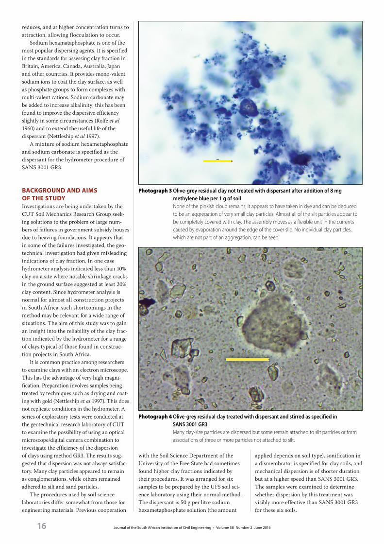
Photograph 1 Olive-grey residual clay not treated with dispersant but mechanically stirred as specified in SANS 3001 GR3 Comparison with the 30 micron by 2 micron rectangle suggests that there are particles of about 2 microns attached to several of the silt particles. Some clay-size particles appear to be dispersed in suspension. note the faint pinkish cloudy patches covering a considerable part of the field of view (most of which is not within the lens’s range of sharp focus).
Photograph 2 Olive-grey residual clay, not treated with dispersant, after addition of 3 mg methylene blue per 1 g of soil Many of the particles of 2 microns and a little larger adhering to the silt particles show a faint blue outline. Much of the pinkish cloudy area has taken in methylene blue and appears to be composed of extremely small clay particles. Little of the field of view is in focus, but some deeply-stained individual particles smaller than 1 micron are discernible.
Journal of the South African Institution of Civil Engineering • Volume 58 Number 2 June 201616
reduces, and at higher concentration turns to attraction, allowing flocculation to occur.
Sodium hexamataphosphate is one of the most popular dispersing agents. It is specified in the standards for assessing clay fraction in Britain, America, Canada, Australia, Japan and other countries. It provides mono-valent sodium ions to coat the clay surface, as well as phosphate groups to form complexes with multi-valent cations. Sodium carbonate may be added to increase alkalinity; this has been found to improve the dispersive efficiency slightly in some circumstances (Rolfe et al 1960) and to extend the useful life of the dispersant (Nettleship et al 1997).
A mixture of sodium hexametaphosphate and sodium carbonate is specified as the dispersant for the hydrometer procedure of SANS 3001 GR3.
bAckGrouNd ANd AIMS of the StudyInvestigations are being undertaken by the CUT Soil Mechanics Research Group seek-ing solutions to the problem of large num-bers of failures in government subsidy houses due to heaving foundations. It appears that in some of the failures investigated, the geo-technical investigation had given misleading indications of clay fraction. In one case hydrometer analysis indicated less than 10% clay on a site where notable shrinkage cracks in the ground surface suggested at least 20% clay content. Since hydrometer analysis is normal for almost all construction projects in South Africa, such shortcomings in the method may be relevant for a wide range of situations. The aim of this study was to gain an insight into the reliability of the clay frac-tion indicated by the hydrometer for a range of clays typical of those found in construc-tion projects in South Africa.
It is common practice among researchers to examine clays with an electron microscope. This has the advantage of very high magni-fication. Preparation involves samples being treated by techniques such as drying and coat-ing with gold (Nettleship et al 1997). This does not replicate conditions in the hydrometer. A series of exploratory tests were conducted at the geotechnical research laboratory of CUT to examine the possibility of using an optical microscope/digital camera combination to investigate the efficiency of the dispersion of clays using method GR3. The results sug-gested that dispersion was not always satisfac-tory. Many clay particles appeared to remain as conglomerations, while others remained adhered to silt and sand particles.
The procedures used by soil science laboratories differ somewhat from those for engineering materials. Previous cooperation
with the Soil Science Department of the University of the Free State had sometimes found higher clay fractions indicated by their procedures. It was arranged for six samples to be prepared by the UFS soil sci-ence laboratory using their normal method. The dispersant is 50 g per litre sodium hexametaphosphate solution (the amount
applied depends on soil type), sonification in a dismembrator is specified for clay soils, and mechanical dispersion is of shorter duration but at a higher speed than SANS 3001 GR3. The samples were examined to determine whether dispersion by this treatment was visibly more effective than SANS 3001 GR3 for these six soils.
Photograph 3 Olive-grey residual clay not treated with dispersant after addition of 8 mg methylene blue per 1 g of soil none of the pinkish cloud remains, it appears to have taken in dye and can be deduced to be an aggregation of very small clay particles. Almost all of the silt particles appear to be completely covered with clay. The assembly moves as a flexible unit in the currents caused by evaporation around the edge of the cover slip. no individual clay particles, which are not part of an aggregation, can be seen.
Photograph 4 Olive-grey residual clay treated with dispersant and stirred as specified in SANS 3001 GR3 Many clay-size particles are dispersed but some remain attached to silt particles or form associations of three or more particles not attached to silt.

Journal of the South African Institution of Civil Engineering • Volume 58 Number 2 June 2016 17
eQuIPMeNt, MAterIAlS ANd theIr uSAGe IN the INveStIGAtIoN
Microscope and cameraAn optical microscope with objectives of 10x, 40x, 60x and 100x was equipped
with a digital camera (resolution 9 mega pixels). Magnification resulting from the combined effects of the microscope’s lenses and the camera was assessed by measurements on a 100 lines/mm diffraction grating.
A drop of sample prepared for hydrome-ter analysis was placed on a microscope slide, covered with a cover-slip and photographed at various magnifications.
Photographs were taken at various loca-tions on the slide. Most of the photographs in this investigation were taken using the microscope’s 40x objective since more pow-erful lenses give a very small depth of focus.
MagnificationThe combined optical and digital magnifica-tion can be defined in different ways. The computer screen that was used to view the images showed lines spaced at 10 microns on the diffraction grating, spaced at 40 mm on the screen when using the 40x objective. This implies a magnification of 4 000 times. Alternatively, the 10-micron spacing on the diffraction grating corresponds to 150 pixels on the photographs produced by the camera using the same objective. The most convenient way of indicating magnification is by incorporating a reference object of known size. All of the photographs in this article have a rectangle superimposed to indicate the scale. The length and breadth of each rectangle represent 30 microns and 2 microns respectively.
variations in procedureSamples were also prepared employing vari-ations to the normal procedures in order to examine the influence of time of soaking in dispersant, time of agitation, concentration of dispersant and volume of dispersant used. Method GR3 specifies only minimum times of soaking and agitation. All of the times involved are within these specifications, and this part of the investigation served only to verify whether this aspect of the specification is adequate. Examination of the concentration of dispersant was prompted by the finding of a difference in hydrometer yield for certain clays using the Japanese and American standards, which specify different concentrations of sodium hexametaphos-phate (Mishra et al 2011).
Methylene blueIn addition, samples were treated with methylene blue (MB), with the aim of labelling clay particles for positive identi-fication. Methylene blue (C16H18 N3SCl) is an effective indicator of clay, as it readily exchanges places with cations in the clay mineral structure, the amount depending on the cation exchange capacity (CEC) and specific surface area (SSA) of the clay min-erals (Turoz & Tosun 2011). Active clays like montmorillonite have high CEC and SSA, and readily take in methylene blue. When MB is available in large concentrations,
Photograph 5 Olive-grey residual clay treated with dispersant and methylene blue The small agglomerations of clay-size particles show little, if any, staining, suggesting very low CEC. The silt particle at bottom centre appears to be coated with very small, high CEC particles which are very darkly stained. The deeply stained agglomeration in the centre is about 50 microns in length and 25 microns in width. It appears to be made of very small, high CEC particles, and it seems to engulf several silt and clay-size particles. Such agglomerations were not uncommon in this sample, but probably not common enough to ensure a meaningless clay fraction from hydrometer analysis.
Photograph 6 Red-brown soil from Limpopo after mechanical stirring without addition of dispersing agent Many of the silt-sized particles appear to have clay-sized particles adhering to them. A faint cloudy pinkish haze, as noted in Photograph 1, is again evident. Most of the silt particles appear to be clustered together in loose associations.
Journal of the South African Institution of Civil Engineering • Volume 58 Number 2 June 201618
such clays rapidly become totally opaque and appear in photographs as dark blobs in which no structure can be seen. Inactive clay minerals like kaolinite have low CEC and SSA and show little colouring until high CEC/SSA fractions present are already deeply stained. Progressive addition of small amounts of dye can therefore give an indi-cation of the types of clay mineral present in a sample, and can also help to establish whether the clay-size particles which can be seen adhering to silt and sand particles are, in fact, composed of clay minerals. Any additive to the soil solution which affects the cation balance will inevitably influence the effectiveness of the dispersant. Only small quantities of methylene blue were therefore added to the dispersed samples. It could be expected that silt and sand would not be coloured, and high CEC / high SSA clays (e.g. montmorillonite) would be col-oured after adding very little dye, whereas low CEC / low SSA clays (e.g. kaolinite) would be coloured only after the addition of considerably more dye.
theoretIcAl coNSIderAtIoNS ANd StreNGthS / weAkNeSSeS of the Method eMPloyedSoil mechanics and soil science generally consider all particles of 2 microns and smaller to be clay-size particles, and those from 2 microns to 60 microns (or some other arbitrary figure of this order) to be of silt-size. But particles and agglomera-tions of clay minerals typically range from about 0.1 micron to slightly more than 2 microns; non-clay particles typically range from about 1 micron upwards (Robinet et al 2011). Some clays, e.g. kaolinite and haloysite, may have particles considerably larger than 2 microns, as can be seen in electron micrographs by Bühmann and Kirsten (1991). There is thus a range where size classification may not correspond with mineral classification. Certain important aspects of soil behaviour (e.g. volume change) depend on clay mineral content, while hydrometer and pipette analyses attempt to establish only particle sizes, not mineral content. Many of the individual particles observed were in this ambigu-ous range of 1 to 2 microns, raising the question of whether they are clay particles which need to be dispersed, or silt particles which do not flocculate and should not need dispersion.
The magnifications possible with the optical microscope and camera combina-tion used in this investigation are probably sufficient to distinguish most of the range typical for clay through silt to sand, but not
adequate to measure the smallest particles in this range. Since all samples remained in aqueous suspension, all of the smaller indi-vidual particles were subject to Brownian motion. At the highest magnification (100x objective – 37.5 pixels per micron, 10 000x magnification on the computer screen), particles at the lower end of the clay-size range could be distinguished in many of the samples, but their Brownian motion
hindered observation or measurement since they suddenly appear in the focal plane, and disappear as they move away from the focal plane. Photographing them was not very successful, possibly because the exposure time of the camera/computer combination was too long. Many small particles were vis-ible and could be photographed where they formed part of large agglomerations or were attached to silt or sand particles.
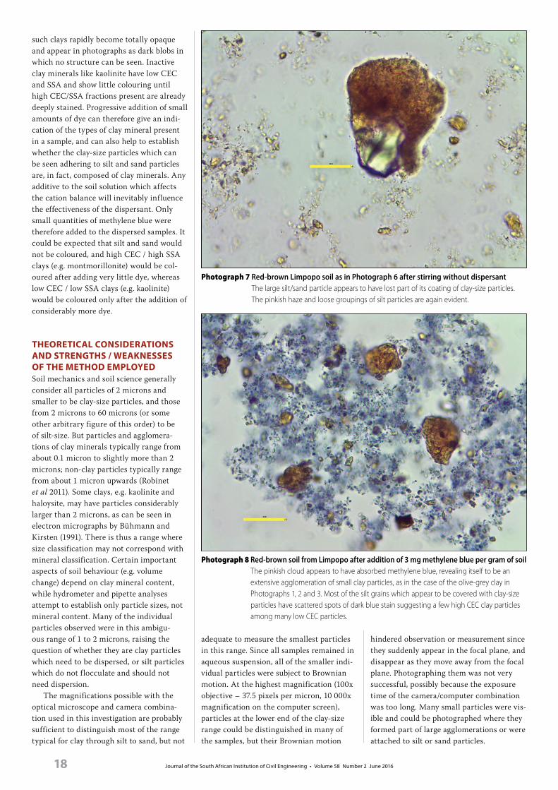
Photograph 7 Red-brown Limpopo soil as in Photograph 6 after stirring without dispersant The large silt/sand particle appears to have lost part of its coating of clay-size particles. The pinkish haze and loose groupings of silt particles are again evident.
Photograph 8 Red-brown soil from Limpopo after addition of 3 mg methylene blue per gram of soil The pinkish cloud appears to have absorbed methylene blue, revealing itself to be an extensive agglomeration of small clay particles, as in the case of the olive-grey clay in Photographs 1, 2 and 3. Most of the silt grains which appear to be covered with clay-size particles have scattered spots of dark blue stain suggesting a few high CEC clay particles among many low CEC particles.

Journal of the South African Institution of Civil Engineering • Volume 58 Number 2 June 2016 19
GeNerAl coNSIderAtIoNSThe following considerations in terms of the microscopic investigation should be noted:1. Those samples extracted for microscopic
investigation at the UFS laboratory were taken by pipette after a settling time calculated to give only silt- and clay-sized particles at the depth of extraction (larger
particles having settled below this level). The largest particle sizes measured were of the order 50 microns, suggesting that the sample was, indeed, restricted to clay and silt-sized particles. Samples prepared in the CUT laboratory were taken imme-diately after agitation, and some samples contained particles considerably larger
than 50 microns, allowing examination of sand grains as well as silt.
2. The cover slip over the sample was supported by the largest particles, and consequently a depth of about 50 microns was filled with suspension for the UFS samples, and up to about 100 microns for the CUT samples. Depth of sharp focus at high magnification is far smaller than this and consequently photographs neces-sarily had most of their field out of focus.
3. Since clay sizes range from 2 microns downwards, the concentration of suspen-sion specified in the hydrometer method allows too many clay particles in a depth of 50 microns for convenient optical differentiation. This made dilution of the hydrometer samples necessary. The majority of samples were diluted with three times their own volume of de-ion-ised water. This dilution was arbitrarily chosen and was considered adequate for this purely qualitative investigation.
4. The gap of approximately 50 to 100 microns between slide and cover slip allows evaporation of the suspension’s water around the edges. It may be pos-sible to seal around the edge of the cover slip and prevent evaporation, but it was found that the movement of water caused by evaporation was helpful in distinguish-ing between clay-size particles which were dispersed and free-floating, and those which were attached to silt or sand particles or formed agglomerations with other clay particles. This consideration results in a very limited time available for the observation of each slide.
5. When samples dry out they conglomer-ate, making it difficult to draw conclu-sions about the behaviour of the clay in conditions relevant to the pipette and hydrometer tests. Only observations in suspension conditions were considered in this investigation.
SAMPleS uSed IN the INveStIGAtIoNSamples of six widely different clay soils (from the Free State, Northern Cape, Western Cape and Limpopo) were mechani-cally agitated, as in procedure GR3, but without first soaking in dispersant. Samples of the same soils were prepared with both dispersant and mechanical agitation at CUT, as per SANS 3001 GR3, and at the Soil Science Laboratory of UFS using standard soil science procedures. From the six soils, two were selected as showing typical features and illustrating the general effectiveness of the investigation’s procedures. One soil appeared to show fair dispersion, the other
Photograph 9 Red-brown Limpopo soil mechanically stirred (without treatment with dispersant) and subsequent addition of 6 mg of methylene blue per gram of soil The dense mass of deeply stained clay particles appears to almost completely engulf a silt particle covered with barely stained clay-size particles.
Photograph 10 Red-brown Limpopo soil not treated by dispersant with 6 mg/g methylene blue added The large blue structure is more than 150 microns by 50 microns in size. Within this structure silt particles can be distinguished. Much of the agglomeration appears to consist of clay particles of about 1 micron or smaller. The agglomeration slightly above and left of centre appears to consist almost entirely of a different species of clay particles of about 2 microns which are very lightly stained. Very few soil particles are visible which are not part of an agglomeration.

Journal of the South African Institution of Civil Engineering • Volume 58 Number 2 June 201620
very inadequate dispersion. The first of these samples is shown in Photographs 1 to 5, the second in Photographs 6 to 13. They provide a reference frame and show widely different clays with and without dispersant, both with and without methylene blue. Features of some of the other soils are shown in the remainder of the photographs.
obServAtIoNSPhotograph 1 is of an olive-grey residual clay from a proposed housing development in Bloemfontein. Tests at the UFS Soil Science Laboratory gave LL 72, PI 26 and clay frac-tion 41% (by both hydrometer and pipette methods). Photograph 2 shows the same sample after the addition of 3 mg of MB per gram of soil. Photograph 3 shows the same sample after the addition of a further 5 mg/g of MB dye.
It appears that a large number of very small clay particles bind considerable numbers of various kinds of particles into associations. Currents caused by evaporation of the suspension’s water show that these associations are flexible, but strongly tied together and move as a unit.
Photograph 4 shows the same soil after treatment with dispersant as specified in SANS 3001 GR3. Comparison with Photograph 1 shows a very large increase in clay-size particles dispersed throughout the water. There are, however, some clay-size particles adhering to silt particles, and a number of small agglomerations of clay-size particles with no visible silt core.
Photograph 5 shows this same dispersant-treated sample after the addition of meth-ylene blue. While this sample shows good dispersion compared to the untreated state, it is apparent that dispersion is not complete. The majority of dispersed particles appear to be about 2 microns in size, but small, deeply stained particles of less than 1 micron can also be seen, and it is difficult to discern whether they are free or attached to larger clay-size particles. The agglomerations of clay-size particles, the clay-coated silt parti-cles and the agglomeration of very fine clay will probably not precipitate at a rate which will ensure their contribution to the clay fraction being recorded by the hydrometer.
Photograph 6 is of a red-brown soil from the Limpopo Province, which has a history of giving variable results in soil tests and caus-ing difficulties in construction. Treatment was only mechanical stirring of the raw soil without dispersant. Commercial laboratory results for samples sent by CUT as part of a parallel testing programme ranged between 17% and 56% for clay fraction, and between 31 and 43 for PI.
As in the case of the olive-grey Bloemfontein soil there are shadowy pinkish bands associated with the distinctly visible particles. There are also many clay-size particles adhering to most of the silt-size particles.
In Photograph 7 a large grain of silt appears to be mostly covered with clay-size particles. Part of the grain, however, is com-pletely clean and free from clay coating. It is possible that it was struck by one of the pad-dles of the mechanical stirrer and some of the coating was torn away. The coating of the lower right area seems to have come loose
from the large particle, but remains attached to the clay coating above.
Photograph 8 shows the same sample after addition of 3 mg/g of methylene blue. A few small blue spots are visible on the larger silt-sized particles, but the majority of par-ticles of about 2 microns remain unstained. A clearly visible cloud of very small blue-stained particles has largely replaced the faint pink cloud, suggesting that the cloud consists of very small and possibly translu-cent clay particles with high CEC/SSA.
Photographs 9 and 10 show the same sample after the addition of a further 3 mg/g
Photograph 11 Red-brown Limpopo soil after treatment with dispersant at the UFS Soil Science Laboratory Many clay-size particles are well dispersed, but a substantial number remain attached to silt particles. There are also cloudy pinkish areas similar to those in Photograph 1.
Photograph 12 Same sample as Photograph 11 after addition of methylene blue

Journal of the South African Institution of Civil Engineering • Volume 58 Number 2 June 2016 21
of methylene blue. Photograph 9 shows a grain of silt, apparently covered with low CEC clay, almost completely enveloped by high CEC clay particles. A number of small clay particles appear to be dispersed into the surrounding water, but the majority are asso-ciated with aggregations. In Photograph 10 a large agglomeration of clay appears to contain several small silt particles of various types.
Photograph 11 shows a sample of the same soil treated with dispersant. Many
small clay particles are dispersed, and, com-pared to Photographs 6 and 7, the groupings of silt particles have largely disappeared. Yet many of the slit particles remain totally or partially coated with clay-size particles, and many agglomerations of two or more clay-size particles can be seen.
Photographs 12 and 13 show the same soil after addition of methylene blue. Compared to Photographs 9 and 10, where no dispersant was used, dispersion is clearly
improved, but most of the silt particles are seen to be covered with clay, and the faint pinkish clouds again appear to be revealing themselves as very fine clay particles which are not well dispersed and may settle in the hydrometer as silt-size aggregates rather than as individual clay particles.
Photograph 13 shows an exceptionally large agglomeration of small clay particles engulfing several silt particles and numer-ous 1 to 2 micron clay particles against a background of well-dispersed clay particles. Nettleship et al (1997) came to the conclusion that their anomalous observations of settle-ment in the hydrometer might be explained by agglomeration taking place while particles were settling during the test. It seems more likely that this could be the case here than that such an agglomeration could have sur-vived 15 minutes of stirring at 1 500 rpm after prolonged soaking in dispersant.
The amount of clay which is obviously not dispersed in Photographs 12 and 13 sug-gests that it is very unlikely that the hydro-meter will give a reliable estimate of the true clay fraction of this soil.
Photograph 14 shows a soil from a housing project in the Northern Cape. Hydrometer analysis had shown the clay fraction for almost all of the samples from this site to be very low. This led to a low value of Van der Merwe’s predicted heave being accepted for design. Heave damage did, however, occur on the project.
A considerable fraction of the clay-size particles visible in the photograph are attached to silt particles of various sizes. It is not clear whether all the agglomerations of clay-size particles have a silt core, but it appears that much of the clay in this sample has not been dispersed. Hydrometer analysis could underes-timate the clay content quite drastically. This might explain the unexpected damage which occurred at the housing project.
Another sample, from less than 100 m away, was prepared according to SANS 3001 GR3 at the CUT laboratory. A house had become structurally unsound due to heave while still under construction a few metres from where this sample was taken. Photographs 15 and 16 are of this sample. In Photograph 15 many of the visible clay-sized particles are attached to silt particles. It appears that the large congregation of clay-sized particles in Photograph 16 surrounds a root hair or similar thin, thread-like structure.
Considerably more clay is undispersed than is dispersed. This would suggest the likelihood of a misleading estimate of clay fraction by the hydrometer method.
Photograph 17 shows a low-activity kaolinitic soil described as “light yellow silty clay” from the Western Cape after
Photograph 13 Same sample as Photograph 12 The dispersion and agitation procedures have produced many well-dispersed clay particles, but the large agglomeration shown here is far from dispersed. This sand-size grouping of silt and clay is unlikely to settle at the rate expected of clay, nor are the numerous smaller aggregations.
Photograph 14 Soil from a subsidy housing project in the Northern Cape after treatment with dispersant and mechanical agitation at the UFS Soil Science Laboratory The majority of silt particles remain covered with clay-size particles.

Journal of the South African Institution of Civil Engineering • Volume 58 Number 2 June 201622
dispersion and addition of methylene blue. It has LL 34, PI 13 and LS 4.6 suggesting that its heave potential is very low. All of the clay particles are about 2 micron or slightly larger in size, which is consistent with the clay being kaolinite. This is the only sample tested which showed no small, high CEC clay particles; all of the other samples showed a range of sizes and probable clay mineral types. Many agglomerations of clay particles are evident. Since it is unlikely that these will settle at the rate expected of individual clay particles, the clay fraction determination is again likely to be unreliable. The description “silty clay” seems inappropriate, since little, if any, silt is evident. The agglomerations of clay are, however, of silt size and it could be that they had settled in the hydrometer at the rate expected of silt-size particles and had been incorrectly assessed as silt.
AddItIoNAl teStSAlthough it appears that one or two of the samples tested showed fair dispersion (as in Photographs 4 and 5), none showed unques-tionably satisfactory dispersion (i.e. little or no clay-sized material forming agglomera-tions or associations with other particles). Some showed very poor dispersion (as in Photographs 12 to 16). Tests at the CUT geotechnical research laboratory were carried out to assess the effect of concentration of dispersant, volume of dispersant, length of time of submersion in dispersant and time of mechanical agitation. The GR3 procedure includes only minimum times for soaking and agitation, so this served only to check the adequacy of this aspect of the specification.
SANS 3001 GR3 calls for a minimum of 16 hours submersion in the dispersing agent. Various periods from 16 hours to 2 weeks were tested. No visible improvement in dis-persion was observed.
SANS 3001 GR3 calls for a minimum mechanical stirring time of 15 minutes at 1 500 rpm. Various periods from 15 min-utes to 24 hours were tried with no visible improvement in dispersion observed. This tends to confirm that the specified minimum times are adequate.
No visible improvement in dispersion was observed by doubling the quantity of disper-sant used to treat the samples or by increasing the concentration of dispersant from 40 g/l to 60 g/l. This was not unexpected, since the UFS samples used 50 g/l and showed no visibly significant improvement in dispersion from the GR3 samples.
Samples taken from suspensions permit-ting little time for settlement, allowed assess-ment of the dispersion of clay particles from sand-size particles. Dispersion appeared to
be no better than from silt, as can be seen in Photograph 18.
With particles as large as this, the depth of the suspension between slide and cover slip is so great that very little of the sus-pended material is in focus. It appears that treatment with dispersant and subsequent
mechanical agitation had failed to dislodge clay particles from the sand grain.
dIScuSSIoNAll of the clays tested showed some lack of dispersion. Every sample showed instances
Photograph 15 Sample of soil from the Northern Cape after soaking in dispersant and mechanical agitation as specified by SANS 3001 GR3 This sample was taken a few metres from where a house became structurally unsound due to heave and was demolished before the roof was installed. Soil apparently identical to this from a nearby test pit was assessed by hydrometer as containing only 6% clay. Many apparently clean silt particles can be seen, as can many dispersed particles smaller than 2 microns. The larger particles are all covered with clay-size particles.
Photograph 16 Same sample as Photograph 15 after treatment with dispersant and mechanical stirring A large number of clay-size particles form an agglomeration around a thin, thread-like structure – possibly a root-hair – while towards the top right many similar size particles appear to be well dispersed.

Journal of the South African Institution of Civil Engineering • Volume 58 Number 2 June 2016 23
of clay remaining attached to larger parti-cles or forming agglomerations with other clay particles.
In some cases the lack of dispersion was fairly small, but in some cases a substantial fraction of the clay particles appeared to be undispersed. This suggests that it will not be reasonable to look for some universal factor
by which hydrometer results could be cor-rected. It appears that predictions based on clay fraction determined by the procedure of SANS 3001 GR3 may be very unreli-able for some soils. Since the SANS 3001 procedure is quite similar to that of many other countries, it is likely that this problem may be widespread. The samples prepared at
the UFS Soil Science Laboratory, using soil science procedures with some differences to those of SANS 3001 GR3, showed visibly similar results to those prepared at the CUT laboratory using the GR3 procedure.
It might be reasonable to consider specify-ing different de-flocculants for different types of soil. Rodriguez et al (2011) found that lith-ium hydroxide is very efficient for high-CEC soils, but is not effective for dispersing low-CEC electropositive soils. Rolfe et al (1960) found considerable difference in the clay yield given by a number of dispersants across different types of clay in hydrometer tests. Perhaps it is not surprising that the single dispersant specified for all South African soils appears to be reasonably adequate for some soils and completely inadequate for others. Changing dispersant may be futile, however, since most of the soils tested showed mixtures of clay ranging from small, high CEC particles (much of it probably montmorillonite) to large, low CEC particles (much of it probably kaolinite). If a dispersant is not efficient for several types of clay, it will not give reliable results for these soils.
The methods of quantitatively assessing the efficiency of de-flocculants for geotech-nical and soil-science purposes (Rodriguez et al 2011; Rolfe et al 1960) take hydrometer yield as the standard of comparison. There appears to have been no attempt to assess how much of the clay remains undispersed. The use of even the most efficient dispersant for any particular clay may therefore give poor results.
There is also the question of mechanical agitation. Rodriguez et al (2011) noted that horizontal mechanical shaking in helicoidal motion, with the addition of coarse sand as an abrasive, is more effective for dispersion than the conventional method. They did note, however, that its efficiency is not the same for all soils.
coNcluSIoNIt appears that Savage’s suspicion that “de-flocculation of many clays is seldom fully completed at the time of testing” is well founded. None of the clays tested reached good dispersion, even when all aspects of the dispersion procedure were extended substantially. Clay coating of large (silt/sand) particles was observed to some extent in all samples which contained silt and sand par-ticles – in some cases to a very considerable extent. Such particles will probably settle at the rate of silt/sand particles and their clay coating will not be assessed with the clay fraction.
It may be advisable to consider the hydrometer unreliable for any critical
Photograph 17 Western Cape yellow kaolinitic soil after addition of methylene blue following treatment with dispersant and mechanical stirring to the specification of SANS 3001 GR3 Almost all of the particles are about 2 microns or slightly larger. Many form groups of from a few to many particles. Many appear to be properly dispersed, but many are not.
Photograph 18 Dark-brown sandy clay from a road project at Thaba Nchu in the central Free State after preparation for hydrometer analysis by soaking in dispersant and mechanical agitation according to SANS 3001 GR3 This sand grain is of the order of 200 microns long and 100 microns wide. It appears to be completely covered with clay-size particles. Many clay particles around it are dispersed, although most are out of focus and cannot be clearly seen.

Journal of the South African Institution of Civil Engineering • Volume 58 Number 2 June 201624
analysis such as heave prediction. Work in progress at the CUT soil mechanics research group is attempting to find more reliable methods of assessing clay frac-tion, but this is at a very early stage and is therefore unlikely to be able to give reliable quantitative results for at least two years. The quest for better methods of assessing clay content should perhaps become a priority on a wider scale.
AckNowledGeMeNtSThe authors wish to express their thanks and appreciation to Prof L van Rensburg and Mrs Y Dessels of the Free State University, and Prof SW Jacobsz of the University of Pretoria, for their assistance and encour-agement, as well as the National Research Foundation (NRF) for its financial sup-port of the CUT soil mechanics research group’s work.
refereNceSAl-Lami, H S 2008. Evaluation of some water-soluble
dispersants for different types of kaolin powders.
Al-Taqani, 21: 95–100. Available at: http://www.iasj.
net.
Bühmann, C & Kirsten W F A 1991. The mineralogy of
five weathering profiles, developed from Archaean
granite in the eastern Transvaal, Republic of South
Africa. South African Journal of Plant and Soil,
3: 126–152. DOI: 10.1080/02571862.1991.10634823.
Das, B M 2008. Advanced Soil Mechanics, 3rd ed. New
York: Taylor and Francis.
Konert, M & Vandenberghe, J 1997. Comparison of laser
grain size analysis with pipette and sieve analysis: A
solution for the underestimation of the clay fraction.
Sedimentology, 44(3): 523–535.
Ma, Z, Merkus, H G, de Smet, J G A E, Heffels, C &
Scarlett, B 2000. New developments in particle
characterization by laser diffraction: Size and shape.
Powder Technology, 111(1–2): 66–78.
McCave, I N, Bryant, R J, Cook, H F & Coughanowr,
C A 1986. Evaluation of a laser-diffraction-size
analyser for use with natural sediments. Journal of
Sedimentary Petrology, 56(4): 561–564.
Mishra, A K, Ridlo, M O & Higashi, T 2011.
Comparison of the clay fraction of Ariake clay
determined by Japanese and ASTM standards.
Marine Georesources and Geotechnology, 29(2):
110–116. DOI: 10.1080/1064119X.2012.525138.
29:110-116, 2011.
Nettleship, I, Cisko, L & Vallejo, L E 1997. Aggregation
of clay in the hydrometer test. Canadian
Geotechnical Journal, 34: 621–626.
Robinet, J C, Coelho, D & Altmann, S 2011. State of
the art on cation diffusion in clay mineral systems.
Karlsruhe, Germany: European Commission
(Community Research), CatClay Report 1/5/2011.
Rodrigues, C, de Oliveira, V A, da Silveira, P M &
Santos, G G 2011. Chemical dispersants and pre-
treatments to determine clay in soils with different
mineralogy. Journal of the Brazilian Society of Soil
Science, 35(5): 1589–1596. Available at: http://www.
redalyc.org.
Rolfe, B N, Miller, R F & McQueen, I S 1960. Dispersion
characteristics of montmorillonite, kaolinite, and
illite clays in waters of varying quality, and their
control with phosphate dispersants. Washington DC:
Geological Survey and Colorado State University,
Professional Paper 334-G.
SANS (South African National Standard) 2011. SANS
3001: 2011, Edition 1.1. Civil Engineering Test Methods,
Part GR3. Pretoria: SABS Standards Division.
Savage, P F 2007. Evaluation of possible swelling
potential of soil. Proceedings, 26th South African
Transport Conference (SATC 2007), Pretoria, 9–12
July 2007.
Skempton, A W 1953. The colloidal “activity” of clays.
Proceedings, 3rd International Conference on Soil
Mechanics, Zurich, 1, pp 57–60.
Turoz, M & Tosun, H 2011. The use of methylene blue
test for predicting swell parameters of natural clay
soils. Scientific Research and Essays, 8: 1780–1792.
Van der Merwe, D H 1964. The prediction of heave
from the plasticity index and percentage clay
fraction in soils. The Civil Engineer in South Africa,
June: 103–107.
Zschimmer & Schwarz GmbH & Co 2014. Mechanisms
of action of deflocculates and dispersants in
ceramic bodies. Ceramics. Available at: http://www.
zschimmer-schwarz.com/en/simon/zschimmer-
schwarz/media/site/downloads/fachinfo/eng/
Fach/E_WirkmechVerfluess.pdf.

25Jones BR, Jacobsz SW, Van Rooy JL. A qualitative model study on the effect of geosynthetic foundation reinforcement in sand overlying very soft clay. J. S. Afr. Inst. Civ. Eng. 2016;58(2), Art. #1340, 10 pages. http://dx.doi.org/10.17159/2309-8775/2016/v58n2a3
techNIcAl PAPerJournal of the South african inStitution of civil engineeringVol 58 No 2, June 2016, Pages 25–34, Paper 1340
BREnDOn JOnES completed his BSc (Hons) degree at the University of KwaZulu-natal in 2010, joining the consulting industry thereafter, and currently he is with SMEC South Africa. In 2014 he graduated with an MSc in Engineering Geology from the University of Pretoria. He has been involved in academia as a part-time lecturer at the University of Pretoria and is
studying towards his PhD at the same institution.
Contact details: Department of Geology University of Pretoria Private Bag X20 Hatfield, 0028 South Africa T: +27 12 420 5012 E: [email protected]
PROF S W Jacobsz (Pr Eng, MSAICE) graduated with an MEng degree from the University of Pretoria in 1996 and completed a PhD at the University of Cambridge in 2002. He is an associate professor in the Department of Civil Engineering at the University of Pretoria, and has 20 years of design and research experience in industry and academia.
Contact details: Department of Civil Engineering University of Pretoria Pretoria, 0002 South Africa T: +27 12 420 3124 E: [email protected]
PROF LOUIS VAn ROOY started lecturing in the Department of Geology at the University of Pretoria in 1985, obtaining his PhD in Engineering Geology in 1992. His research interests include the durability of basic igneous rocks for use in construction, problem soils, safe development on dolomite land, and rock engineering. He has supervised or
co-supervised more than 25 MSc and PhD students, and is the author or co-author of more than 30 papers in journals and conference proceedings. He serves on the council of SAIEG (South African Institute of Engineering and Environmental Geologists) and is the Vice-President for Africa of IAEG (International Association of Engineering Geologists).
Contact details: Department of Geology University of Pretoria Private Bag X20 Hatfield, 0028 South Africa T: +27 12 420 2023 E: [email protected]
Keywords: centrifuge modelling, soft clay, geogrid, reinforced sand
INtroductIoNSouthern Africa’s eastern coastline is characterised by several lagoonal systems, comprising complex unconsolidated deposits of sands, silts and clays. These river estuaries are hosts to a number of major harbours, and have proved to be problematic as far as foundation solutions for structures, which typically involve piling techniques, are concerned. Zannoni et al (2012) and Moore et al (2012) have both presented case studies where high-tensile strength geogrids have successfully been adopted to provide basal reinforcement upon which structures can be founded. The basal reinforcement utilised in both studies was specifically to support the floors of warehouse structures in which large platform loads developed as a result of product stockpiling. The foundations for the walls and overhead roof structures were piled. The major concern on site for both these studies was the presence of compress-ible, soft, thin, shallow clay horizons below the foundation footprint.
The warehouse floors were constructed on a layer of sand reinforced with a geogrid constructed over the soft clay layer. The application of surcharge to the floor would result in undrained loading of the clay. Increasing the load would eventually result in the undrained strength of the clay being exceeded. This could result in the clay failing by being squeezed out to the sides (SANS 207 2006). This deformation could result in undesirable non-uniform settlement and horizontal deformation of the floor. The intension with the provision of reinforcement
in the sand layer above the clay is to control horizontal deformation and to strengthen the sand layer to provide a more rigid support to the floor.
Deformation observed in soil is the result of both compressive and tensile strains, which usually develop when soil shears (Jewell 1996). However, when reinforce-ment is placed in soil it can develop bond through frictional contact between the soil particles and the planar surface areas of the reinforcement, and from bearing stresses on transverse surfaces that exist in geogrids or ribbed strips (Jewell 1996). Deformation in the soil causes tensile forces to develop in the reinforcement when the reinforcement is inclined in a direction perpendicularly to that of the compressive strain in the soil. The mobilised reinforcement force, ultimately limited by the available bond, acts to alter the force equilibrium in the soil (Jewell 1996). The performance of reinforced soil foundations depends not only on soil and reinforcement properties, but also on this interaction between the soil and reinforcement (Sharma et al 2009). Sharma et al (2009) also noted that geogrids with higher tensile moduli performed better than geogrids with lower moduli, whilst Binquet and Lee (1975) were also the earliest researchers to show that a failure load could be increased by the use of multiple layers of reinforcement.
Sharma et al (2009) summarised three reinforcement mechanisms of a reinforced soil foundation under strip footings. One mechanism, termed the membrane effect, is
A qualitative model study on the effect of geosynthetic foundation reinforcement in sand overlying very soft clayB R Jones, S W Jacobsz, J L van Rooy
A centrifuge model study was carried out investigating the effects of the inclusion of geogrid reinforcement in a sand layer constructed over a thin, very soft clay layer to facilitate the construction of warehouse floors supporting product stockpiles. The use of geogrid reinforcement allowed larger surcharge loads to be applied for a given amount of settlement by allowing load to be spread over the footprint area of the geogrid due to the tension membrane effect and its associated benefits. A lower-bound calculation of the load at which the tensile reinforcement starts to function is presented. Upper-bound solutions were found to overestimate allowable surcharge loads, as they are associated with unacceptable deformations. The reinforcing effect of the geogrid was found to have been fully mobilised at 5% vertical compression of the clay layer.
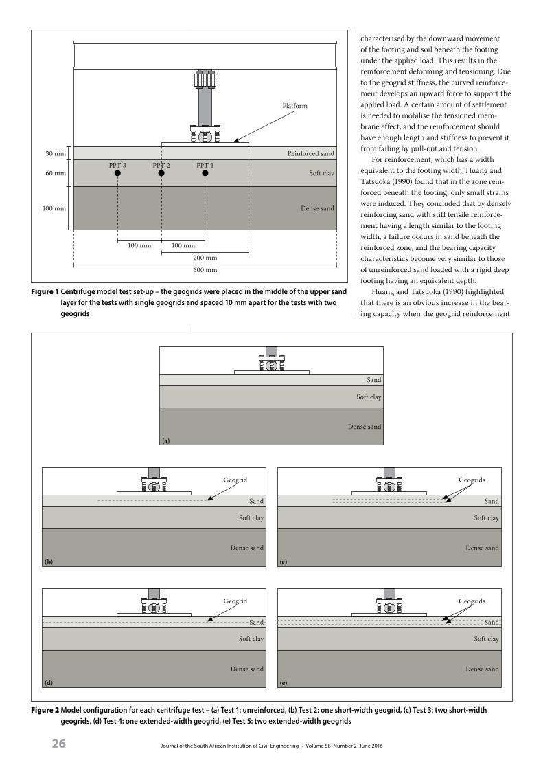
Journal of the South African Institution of Civil Engineering • Volume 58 Number 2 June 201626
characterised by the downward movement of the footing and soil beneath the footing under the applied load. This results in the reinforcement deforming and tensioning. Due to the geogrid stiffness, the curved reinforce-ment develops an upward force to support the applied load. A certain amount of settlement is needed to mobilise the tensioned mem-brane effect, and the reinforcement should have enough length and stiffness to prevent it from failing by pull-out and tension.
For reinforcement, which has a width equivalent to the footing width, Huang and Tatsuoka (1990) found that in the zone rein-forced beneath the footing, only small strains were induced. They concluded that by densely reinforcing sand with stiff tensile reinforce-ment having a length similar to the footing width, a failure occurs in sand beneath the reinforced zone, and the bearing capacity characteristics become very similar to those of unreinforced sand loaded with a rigid deep footing having an equivalent depth.
Huang and Tatsuoka (1990) highlighted that there is an obvious increase in the bear-ing capacity when the geogrid reinforcement
Figure 1 Centrifuge model test set-up – the geogrids were placed in the middle of the upper sand layer for the tests with single geogrids and spaced 10 mm apart for the tests with two geogrids
Platform
100 mm
600 mm
200 mm
100 mm100 mm
60 mm
30 mm
PPT 1PPT 2PPT 3
Reinforced sand
Soft clay
Dense sand
Figure 2 Model configuration for each centrifuge test – (a) Test 1: unreinforced, (b) Test 2: one short-width geogrid, (c) Test 3: two short-width geogrids, (d) Test 4: one extended-width geogrid, (e) Test 5: two extended-width geogrids
Dense sand
Soft clay
Sand
(a)
Dense sand
Soft clay
Sand
(b)
Geogrid
Dense sand
Soft clay
Sand
(c)
Geogrids
Dense sand
Soft clay
Sand
(d)
Geogrid
Dense sand
Soft clay
Sand
(e)
Geogrids

Journal of the South African Institution of Civil Engineering • Volume 58 Number 2 June 2016 27
is wider than the footing width. They suggest that the increase in the bearing capacity, by using long reinforcement layers, can be considered due to two factors – firstly, from the deep footing effect, as is observed in the case of reinforcing with short reinforce-ment layers, and secondly, from the effects contributed by the portions of reinforcement placed in the zone beyond the footing width. They termed this the ‘wide slab’ effect. Their test results showed that the wide slab effect contributed about 10–50% of the total increase in the bearing capacity. Huang and Tatsuoka (1990) also concluded that the degree of contribution also increased with a larger covering ratio above the reinforcement and the number of reinforcing layers present.
Sharma et al (2009) note four possible failure modes for reinforced soil foundations, namely (1) failure above the top layer of reinforcement, (2) failure between reinforce-ment layers, (3) failure similar to footings on a two-layer soil system, and (4) bearing failure within the reinforced zone. Of the four possible modes of failure defined, the third failure mode was the most relevant to the research covered in this paper. This failure mode is applicable to footings on a two-layer soil system, which is similar to when a strong soil layer overlies a weaker soil layer (Wayne et al 1998). This occurs if the strength of the reinforced zone is much larger than that of the underlying unreinforced zone, and the reinforcement depth ratio (d/B) is relatively small. Consequently, a punching shear failure will occur in the reinforced zone, followed by a general shear failure in the underlying softer unreinforced zone (Sharma et al 2009).
Understanding failure mechanisms is an important component of stability analyses of earth structures. If reinforcement is used, the mechanisms become altered, and choosing the right mechanism for stability analysis may not always be straightforward (Michalowski & Shi 2003). This study seeks to qualitatively define the behaviour of a compressible, soft, thin, shallow clay horizon
under an applied load from a wide platform founded upon reinforced sand by using geotechnical centrifuge modelling. Jones and Van Rooy (2014) have previously presented some preliminary findings, and this paper serves to finalise the study.
GeotechNIcAl ceNtrIfuGe Model
test set-upFive geotechnical centrifuge model tests were performed at a scale of 1:50 using the 150 G-ton geotechnical centrifuge housed in the Department of Civil Engineering at the University of Pretoria. Details of the centrifuge facility are described by Jacobsz et al (2014). The model consisted of a 100 mm (5 m) thick dense basal sand layer, overlain by a 60 mm (3 m) thick soft clay layer, which was subsequently overlain by a 30 mm (1.5 m) thick sand layer in which the geogrids were placed. The dimensions in brackets refer to the full scale. Each test was constructed identically, with the model set-up illustrated in Figure 1 and the different configurations of each test illustrated in Figure 2.
The first model (Test 1) was tested without any reinforcement. Tests 2 and 3 consisted of models that were respectively reinforced with one and two geogrids placed in the upper sand layer. The geogrids extended 50 mm (2.5 m) past the edge of the platform and are referred to as having a short width. Tests 4 and 5 had one and two geogrids respectively, extending to 180 mm (9 m) from the edge of the platform, and are referred to as geogrids of extended width. Tests 2 and 4 had one geogrid placed in the middle of the clay layer, while Tests 3 and 5 had two geogrids spaced 10 mm (0.5 m) apart.
Model preparation and constructionThe model was prepared in a strongbox measuring 600 mm x 400 mm in plan, fitted with a glass window, which was reduced to
600 mm x 250 mm by placing spacers at the back of the strongbox. The basal sand layer was pluviated to create a 100 mm (5 m) thick dense sand horizon with a relative density of about 69%. This sand was carefully saturated from the base by introducing pore water via a header tank. Dry kaolin clay powder was pre-pared by mixing under partial vacuum with de-ionised, de-aired water at twice the liquid limit. The slurry was poured over the basal sand horizon and allowed to consolidate in the centrifuge for 14 hours at 50 G under a surcharge load of approximately 25 kPa. This ensured that the clay was normally consoli-dated and of a very soft consistency with an undrained shear strength which averaged approximately 6 kPa in each test (measured using a vane shear apparatus).
Finally, the reinforced sand layer was pluviated over the clay to a thickness of 30 mm (1.5 m). For the tests with reinforcing included, the sand pluviation was ceased tem-porarily to allow placement of the geogrids within the reinforcing sand. The geogrids used were unscaled Macgrid EG 20S (a polypropylene biaxial geogrid produced by an extrusion process), obtained from Maccaferri. The geogrid had an ultimate tensile strength of 20 kN/m at 13% strain, with a stiffness of approximately 350 kN/m, i.e. very stiff and strong at the prototype scale. The mesh open-ing size of the geogrid was 38 mm × 38 mm, and had a percentage open area of 76%. The geotechnical properties of the sand, clay and model geogrid are presented in Table 1, whilst the geogrid is shown in Figure 3.
Three pore pressure transducers (PPTs) were installed at three locations within the clay layer of the model. PPT 1 was installed underneath the centre of the platform, and PPT 2 at the edge of the platform, 100 mm away from the first transducer. PPT 3 was installed 100 mm from the edge of the plat-form. All PPTs were positioned in the middle of the clay layer. The purpose of the PPTs was to assess the extent of the zone influenced due to the application of the platform load, as
Table 1 Geotechnical properties of the materials used in the centrifuge model tests
Sand*Angle of internal friction, φ 34°
Dry unit weight, γd(max) 16.7 kN/m3
Clay
Liquid limit 47%
Plastic limit 22%
Undrained shear strength 6.1 kPa
Saturated unit weight, γs 19.3 kN/m3
GeogridUltimate tensile strength (UTS) 20 kN/m
Strain at UTS 13%
*(Archer 2014)Figure 3 Macgrid EG 20S biaxial geogrid used
in the centrifuge model tests
120 mm80 mm40 mm0 mm

Journal of the South African Institution of Civil Engineering • Volume 58 Number 2 June 201628
loading of the clay would immediately result in the generation of excess pore pressures. Jones (2014) provides further details of the materials and methodology used during the model construction for the centrifuge tests.
test sequenceDuring loading of the model an aluminium platform of 200 mm width, 250 mm length, and 5 mm thickness was attached to a jack and lowered at a constant rate of 0.081 mm/s. The bending stiffness (EI) of the plate was 729 Nm2/m width at the model scale, equiva-lent to 91.2 MNm2/m at full scale. A load cell recorded the applied load mobilised against the platform, while an LVDT measured the vertical displacement at the centre of the platform. The model was observed using a small digital video camera.
ceNtrIfuGe teSt reSultS
load – deformation behaviourThe deformation behaviour from snapshots during each test at respectively 5, 10 and 15 mm vertical displacement is presented in Figures 4, 5 and 6. In order to qualify the deformation behaviour in each model, the following was specifically observed during each test: (1) the mean applied stress recorded against the platform, (2) the maximum vertical height of the heave during deformation of the clay horizon, (3) the offset of this maximum height from the edge of the platform, and (4) the width of the heave zone. A transparency with a grid printed on it was placed between the glass and the model, which assisted in scaling the geometry of the deformation behaviour. Each square on the grid measured 5 mm x 5 mm. Table 2 sum-marises the observations from the deforma-tion of the clay horizon.
Test 1 – unreinforcedIt is evident in Test 1, which had no reinforce-ment, that at 5 mm vertical platform displace-ment there was little deformation of the clay horizon. The applied load was 20.4 kPa. The width of the deformation zone is 320 mm, with a maximum height of heave of 1 mm, and the offset of this maximum height at 40 mm from the edge of the platform.
At 10 mm vertical displacement, under an applied load of 23.8 kPa, a shear zone formed vertically through the upper sand horizon below the edges of the platform as punching occurred into the underlying clay. The clay horizon continued to strain underneath the platform and squeezed out laterally. The width of the deformation zone increased to 380 mm, with the heave in the clay attaining a maximum height of approximately 5 mm.
Figure 4 Comparison of load-deformation behaviour between (a) Test 1: unreinforced, (b) Test 2: one short geogrid, (c) Test 3: two short geogrids, (d) Test 4: one extended geogrid, and (e) Test 5: two extended geogrids, at 5 mm vertical displacement
Legend:A: Reinforcing sand Platform edge: Layer interface:B: Clay layer Geogrid:C: Basal sand Width of deformation: Maximum heave:
Test 524.8 kPa
Test 422.5 kPa
Test 314.4 kPa
Test 228.9 kPa
Test 120.4 kPa
A
B
C(a)
(b)
(c)
(d)
(e)
Table 2 Observed deformations in the centrifuge model tests at 5, 10 and 15 mm displacement
Test
1 2 3 4 5
5 mm
Applied stress (kPa) 20.4 28.9 14.4 22.5 24.8
Maximum heave height (mm) 1 2 2 1 3
Offset of maximum heave height (mm) 40 70 50 75 70
Overall width of deformation zone (mm) 320 420 360 440 500
10 mm
Applied stress (kPa) 23.8 36 23.2 31.3 34.1
Maximum heave height (mm) 5 4 5 5 9
Offset of maximum heave height (mm) 60 70 75 85 105
Overall width of deformation zone (mm) 380 440 490 460 500
15 mm
Applied stress (kPa) 29.9 44.3 32.5 40.9 44.7
Maximum heave height (mm) 5 6 10 10 14
Offset of maximum heave height (mm) 50 70 75 95 110
Overall width of deformation zone (mm) 450 450 530 520 500

Journal of the South African Institution of Civil Engineering • Volume 58 Number 2 June 2016 29
The extent of the deformation zone of the clay at 15 mm vertical displace-ment had increased in width to 450 mm. The maximum height of heave occurred approximately 50 mm from the edge of the platform. However, there was no change in the height of heave as it remained at a maxi-mum of 5 mm. The load at this time reached 29.9 kPa. In this test the largest strains in the clay appeared to occur immediately under-neath the footprint of the platform as the platform punched into the clay, displacing clay outwards and upwards, causing some heave at the adjacent surface.
Test 2 – one short-width geogridWith one short-width geogrid in Test 2, there was already some deformation of the
clay horizon present at small displacements, unlike the unreinforced test. At 5 mm verti-cal displacement, the width of the zone of visible deformation was 420 mm, whilst the maximum height of heave was 2 mm, located 70 mm from the edge of the platform. The applied stress achieved at this displacement was 28.9 kPa.
At 10 mm vertical displacement, the width of the deformation zone was 440 mm, whilst the heave of the clay horizon attained a maximum height of approximately 4 mm at an offset which remained at 70 mm. The applied stress achieved was 36 kPa.
The lateral extent of the deformation zone, as well as the offset of the maximum height of heave of the clay, was the same at 15 mm vertical displacement. However, the
maximum height of heave was 6 mm for the clay horizon, by which time the applied stress had increased to 44.3 kPa. The clay below the width of the geogrid had exhibited the most strain.
Test 3 – two short-width geogridsTest 3, which had two short-width geogrids, much like in Test 2, showed some deformation of the clay horizon at 5 mm vertical platform displacement at an applied stress of only 14.4 kPa. Reasons for this low stress are possibly related to poor saturation of the clay, as will be discussed later. The heave attained a maximum height of 2 mm at an offset of 50 mm, and the width of the visible deformation zone amounted to 360 mm.
At 10 mm vertical displacement, under an applied stress of 23.2 kPa, the heave of the clay reached a maximum height of approximately 5 mm at an offset of 75 mm, whilst the width of the deformation zone had increased to 490 mm.
The width of the deformation zone of the clay at 15 mm vertical displacement increased to 530 mm. While the offset at which maximum heave occurred, remained unchanged at 75 mm from the edge of the platform, the heave attained a maximum height of 10 mm at an applied stress of 32.5 kPa. Similar to the test with a single layer of short-width geogrid, the largest strains that had occurred in the clay horizon coincided with the width of the geogrid.
Test 4 – one extended-width geogridThe model with a single layer of extended-width geogrid showed little deformation of the clay horizon at 5 mm vertical displace-ment. The mobilised stress at this time was 22.5 kPa and the width of the deformation zone approximately 440 mm, with the offset of the maximum height of heave occurring 75 mm from the platform edge. The height of heave was only 1 mm.
At 10 mm vertical displacement, the width of the deformation zone had reached 460 mm, while the heave of the clay reached a maximum height of approximately 5 mm. The offset had moved to 85 mm from the edge of the platform and the mobilised stress had increased to 31.3 kPa.
At 15 mm vertical displacement the lateral extent of the deformation zone of the clay was wider (520 mm). The heave attained a maximum height of 10 mm at an offset of 95 mm, under an applied mobilised load of 40.9 kPa. The inclusion of the single extended-width geogrid reinforcement in the sand in the upper horizon widened the zone of deformation in the clay to a width coincid-ing with the width of the geogrid.
Figure 5 Comparison of load-deformation behaviour between (a) Test 1: unreinforced, (b) Test 2: one short geogrid, (c) Test 3: two short geogrids, (d) Test 4: one extended geogrid, and (e) Test 5: two extended geogrids, at 10 mm vertical displacement
Legend:A: Reinforcing sand Platform edge: Layer interface:B: Clay layer Geogrid:C: Basal sand Width of deformation: Maximum heave:
Test 534.1 kPa
Test 431.3 kPa
Test 323.2 kPa
Test 236.0 kPa
Test 123.8 kPa
A
B
C(a)
(b)
(c)
(d)
(e)

Journal of the South African Institution of Civil Engineering • Volume 58 Number 2 June 201630
Figure 6 Comparison of load-deformation behaviour between (a) Test 1: unreinforced, (b) Test 2: one short geogrid, (c) Test 3: two short geogrids, (d) Test 4: one extended geogrid, and (e) Test 5: two extended geogrids, at 15 mm vertical displacement
Legend:A: Reinforcing sand Platform edge: Layer interface:B: Clay layer Geogrid:C: Basal sand Width of deformation: Maximum heave:
Test 544.7 kPa
Test 440.9 kPa
Test 332.5 kPa
Test 244.3 kPa
Test 129.9 kPa
A
B
C(a)
(b)
(c)
(d)
(e)
Test 5 – two extended-width geogridsTest 5, with two extended-width geogrids, showed some deformation and heave of the clay horizon occurring at 5 mm verti-cal displacement. The deformation zone attained a width of approximately 500 mm and the heave attained a maximum height of 3 mm, 70 mm from the platform edge. This occurred at an applied stress of 24.8 kPa.
At 10 mm vertical displacement, the hori-zontal extent of the deformation zone did not change. However, the heave of the clay reached a maximum height of approximately 9 mm, 105 mm from the platform edge. The mobilised stress had increased to 34.1 kPa.
At 15 mm vertical displacement, the heave attained a maximum height of 14 mm, with the offset increasing to 110 mm from the platform edge. The mobilised stress reached 44.7 kPa. Again, most of the defor-mation in the clay coincided with the width of the reinforcement.
Platform load – settlement behaviourThe loads mobilised against the platform during each centrifuge model test are plotted against the vertical platform displacement in Figure 7. The corresponding applied stresses are also indicated.
Looking at Figure 7, the loads from Tests 1, 2, 4 and 5 (i.e. the tests without reinforce-ment, with one short geogrid, and with one and two extended geogrids respectively) initially mobilised at very similar rates. The results from Test 3 (two short geogrids) show a very soft response and it is thought that the clay in this test might have been poorly con-solidated or not thoroughly saturated, which makes comparison with the other test results difficult. This test result is therefore gener-ally excluded from the discussions below.
The effect of the inclusion of reinforce-ment becomes evident after approximately 3 mm of settlement. This illustrates that some settlement is required before tensile strength is mobilised in the reinforcement. In the case of the unreinforced situation, the rate at which load is mobilised with settle-ment is visibly lower than for the reinforced cases beyond 3 mm settlement. This illus-trates the stiffening effect provided by the reinforcement.
The results from the tests on extended geogrids (Tests 4 and 5) are very similar, with Test 5, which had two geogrids, ultimately mobilising a slightly higher load than Test 4.
load – pore pressureIt was of interest to know the extent of the zone of influence resulting from the loading of the platform as a function of the Figure 7 Load-displacement curves for the centrifuge model tests, up to 15 mm vertical displacement
Load
(kN
)
2.5
2.0
1.5
1.0
0.5
0
Displacement (mm)1514131211109876543210
App
lied
stre
ss (k
Pa)
50
45
40
35
30
25
20
15
10
5
0
Test 1: Unreinforced Test 2: One geogrid (short)Test 4: One geogrid (extended)
Test 3: Two geogrids (short)Test 5: Two geogrids (extended)

Journal of the South African Institution of Civil Engineering • Volume 58 Number 2 June 2016 31
reinforcement layout used. Load application during the centrifuge tests was rapid to model undrained construction. Undrained loading of the clay layer would have been accompanied by immediate changes in pore pressures. The magnitude of the excess pore pressures generated indicates the magnitude of total stress change acting at each particu-lar location. Pore pressures were therefore measured at three different locations within the clay layer (illustrated in Figure 8(f)) to judge the extent of the zone of influence.
The change in pore pressure measured at three different locations with respect to the platform during each test, plotted against the applied stresses, are displayed in Figure 8. A 45° line is indicated for each test result,
indicating an excess pore pressure or total stress change equal to the magnitude of the applied stress.
Figure 8(a) shows the pore pressures generated in the test without reinforcement (Test 1). The pore pressure response under the centre of the platform was initially very similar to the applied stress, up to an applied stress of about 18 kPa, due to undrained conditions. The pore pressure response under the edge of the platform was less, reflecting the reduced stress increase below the edge, as expected. The pore pressure at PPT3, located 100 mm from the edge of the platform, initially showed no response, but then suddenly began to increase beyond about 18 kPa applied stress at a rate similar
to the rate of load application. That seems to suggest that the clay under the platform yielded at this point, mobilising a failure mechanism, suddenly expanding the zone of influence. This hypothesis is supported when comparing with Figure 7, where an applied stress of 18 kPa corresponds well with the point on the stress-settlement curve where the rate of settlement versus applied stress increased. The corresponding settlement was approximately 3 mm (5% of the depth of the clay layer).
Figure 8(b) (Test 2) illustrates the effect of the inclusion of reinforcement. The pore pressure response was initially very similar to that of Test 1, but PPT3 began to respond significantly earlier. This illustrates that
Figure 8 Change in pore pressure versus load curves, for each centrifuge model test
∆ P
ress
ure
(kPa
)∆
Pre
ssur
e (k
Pa)
∆ P
ress
ure
(kPa
)
∆ P
ress
ure
(kPa
)∆
Pre
ssur
e (k
Pa)
30
30
30
30
30
25
25
25
25
25
20
20
20
20
20
15
15
15
15
15
10
10
10
10
10
5
5
5
5
5
0
0
0
0
0
Applied stress
Applied stress
Applied stress
Applied stress
Applied stress
0
0
0
0
0
10
10
10
10
10
20
20
20
20
20
40
40
40
40
40
30
30
30
30
30
50
50
50
50
50
60
60
60
60
60
(a) Test 1: Unreinforced (b) Test 2: One geogrid (short width)
(c) Test 3: Two geogrids (short width) (d) Test 4: One geogrid (extended width)
(e) Test 5: Two geogrids (extended width) (f) Location of PPTs in clay horizon
100 mm100 mm
PPT 1PPT 2PPT 3
Reinforced sand
Soft clay
Dense sand
PPT 1 PPT 2 PPT 3

Journal of the South African Institution of Civil Engineering • Volume 58 Number 2 June 201632
the reinforcement expanded the zone of influence by loading clay adjacent to the platform. It is also significant to note that the rate of pore pressure increase at PPT3 is much lower than in Test 1, reflecting pre-failure conditions.
In Figure 8(c) (Test 3) it can be seen that the pore pressure response under the platform was significantly less than the magnitude of the applied load. This could indicate that the clay was not well satu-rated, which would explain the anomalous response referred to earlier. Despite this, it is evident that the pore pressures at PPT3 began to respond even earlier than in the case of Test 2, illustrating that the addition of a second layer of reinforcement more effectively expanded the influence zone.
The pore pressure responses at PPT1 and PPT2 with extended geogrids (Tests 4 and 5) were initially similar to Tests 1 and 2, i.e. the response under the platform reflected the applied pressure. However, PPT3 began to respond almost immediately after load appli-cation, illustrating that the wider geogrid was effective in expanding the zone of influ-ence far into the adjacent soil.
The pore pressure at PPT3 reached a peak at an applied stress of between 20 kPa and 25 kPa, and then reduced. When compared with Figure 7, this corresponds well to the point where the rate of settlement accelerated. The pore pressure underneath the platform (PPT1 and PPT2) continued to increase linearly with increasing load. It appears that a failure mechanism was mobilised, inter-secting between PPT2 and PPT3 so that there was minimal effect on PPT3 after mobilisa-tion of the failure mechanism.
theoretIcAl ultIMAte loAd ANd fAIlure MechANISMFor the design of the geogrid-reinforced foundation it is necessary to assess the maximum surcharge that can be applied to
the foundation system. Following SANS 207 (2006) this can be estimated using simpli-fied equilibrium calculations, perhaps more rigorously using the principles of upper- and lower-bound plasticity theory (see for exam-ple Atkinson & Bransby 1978; Atkinson 1981; Calladine 2000), or even more rigorously by means of numerical analysis.
In the case of an upper-bound analysis, a potential failure mechanism is identified and the amount of work done by external loads is equated to the amount of internal work dissipated by the mechanism in order to solve the collapse load. It is assumed that full plastic conditions are developed on all failure surfaces. The resulting estimate gives a non-conservative or upper-bound estimate of the collapse load. Failure mechanisms can be optimised to find the most critical one. For the work presented here, the upper-bound collapse load was estimated using the software Limitstate Geo, which applies an optimisation routine to find the most criti-cal failure mechanism and corresponding collapse load estimate. The optimised upper-bound mechanisms for the unreinforced situation are illustrated in Figure 9. An ulti-mate collapse load of 2.18 kN (model scale) or 43.5 kPa is predicted. When compared to the load displacement curves in Figure 7, this estimate is on the high side and is only reached at large displacements.
For the lower-bound estimate, an equilib-rium stress state that nowhere exceeds the yield criterion, is postulated from which the collapse load is estimated using principles of equilibrium. This provides a conservative estimate of the collapse load. Based on the theory of plasticity, the true collapse load will occur between the upper- and lower-bound estimates. Should the two methods provide identical solutions, an exact solution to the problem would have been found (Atkinson 1981).
A potential lower-bound stress state for a clay layer being compressed between two
rigid surfaces is postulated in Figure 10. The lines forming the patterns of kites and triangles represent stress discontinuities that allow the stress state to vary across discon-tinuities (see for example Bolton (1979) or Atkinson (1981)). In every triangle the major principal stress direction is inclined 30° to the vertical, while in the kites it is vertical. The axis of symmetry of the loaded floor is on the right, with clay being squeezed to the left.
Assuming that the full undrained shear strength of the clay is mobilised in each kite and triangle allows the maximum vertical stress that can be applied to the clay layer to be determined. This maximum vertical stress (σv), i.e. a lower-bound or conservative estimate of the vertical stress required to squeeze out the clay, is given by Equation 1 and increases linearly from the uncon-fined edge at the left to the centre of the loaded area.
σv = √3 cu
D x (1)
where: cu = undrained shear strength of the clay D = thickness of clay layer x = horizontal distance from unconfined
edge
From Equation 1 a lower bound collapse load (Fl) can be estimated as:
Fl = √3
4
cuB2
D (2)
Note that other stress states providing better (i.e. less conservative) lower-bound estimates may be postulated. The lower-bound for the collapse load calculated for the unreinforced situation amounts to 0.433kN. When com-pared with Figure 7, this fits well with the end of the initial linear sections of the load-displacement curves, indicating that this
Figure 9 Most critical upper-bound failure mechanism in the absence of reinforcement (model dimensions)
60 mm
30 mm
200 mm200 mm200 mm
Clay
Sand
43.5 kPa ultimate stress
Rigid footing

Journal of the South African Institution of Civil Engineering • Volume 58 Number 2 June 2016 33
particular lower-bound provides a realistic indication of the first onset of yielding of the clay, i.e. the point at which significant loads will begin to mobilise in the reinforcement.
dIScuSSIoNThis study entailed a qualitative investigation into the effects of using comparatively very strong and stiff geogrid reinforcement on the deformation mechanism below a wide, rigid surcharge on sand overlying soft clay. With the exception of Test 3, which is suspected to have suffered from poor clay saturation, the physical models provided consistent results to allow the effect of different reinforcement configurations to be assessed.
In all the centrifuge model tests there was no disturbance to the boundary between the basal sand horizon and the overlying clay horizon. As such, the interface between the two horizons behaved as a fixed boundary. The clay above the sand moved laterally at this boundary as it was squeezed out from under the applied load. The observed failure modes were typical of a strong soil overlying a weaker soil horizon (Wayne et al 1998).
In the absence of reinforcement, shear planes extending vertically downwards from the edges of the loaded platform soon cut through the sand layer, so that the platform and underlying sand punched into and compressed the clay layer. Heave occurred adjacent to the loaded platform as clay was squeezed out to the sides. At large displace-ments, the extent of the observed zone of influence corresponded well with the extent of the failure mechanism presented in Figure 9.
As expected, the introduction of rein-forcement in the sand layer resulted in higher
loads being mobilised for any given displace-ment (Huang & Tatsuoka 1990). Increasing the amount and extent of the reinforcement resulted in an increased mobilised load for a given displacement. The addition of reinforcement visibly expanded the zone of influence around the loaded platform, with the mode of deformation becoming that of a ‘wide slab’ (Huang & Tatsuoka 1990).
The expansion of the zone of influence was also detected from the pore pres-sure readings. As the platform was forced downward, the geogrids were also stretched downward near the platform, mobilising the tension membrane effect (Sharma et al 2009). This shifted the point of maximum heave further from the platform. At large displacements the width of the zone of influ-ence appeared to be equal to the width of the geogrid. The maximum heave occurred within the width of the reinforcement. If an additional surcharge load can be applied to this region, it may improve the mobilisable tensile resistance of the geogrid by anchoring it more effectively into the sand layer, also potentially mitigating the amount of heave.
The initial load-settlement response from the various tests were very similar, with loads in all tests mobilising approxi-mately linearly, with settlement up to just under 1 mm (1.7% strain in the clay layer). Thereafter, the mobilised load began to flatten off and the load-settlement response became curved. By approximately 3 mm settlement (vertical strain of 5% in the clay layer) the load again increased linearly, with further settlement but at a reduced rate. The end of the initial linear section of the load-settlement curve corresponds well with the lower-bound collapse load calculated above. This lower-bound load was calculated
on the premise that nowhere had yielding of the clay occurred yet. Deformations were subsequently small, and minimal tensile strength would have been mobilised in the reinforcement.
The observation that the load settle-ment curves began to flatten off beyond the lower-bound estimate suggests that yielding had begun to occur. The onset of yielding, i.e. appreciable deformation of the clay, is required for the mobilisation of significant tension in the reinforcement. The flattening off of the curves beyond 3 mm (5% vertical strain in the clay) suggests that the full load that could be transferred to the reinforce-ment had been mobilised. Beyond this point the unreinforced model behaved plastically, with only a very gradual increase in load with further settlement as the loaded plat-form penetrated deeper into the underlying material. The reinforced models showed an increase in load beyond this point as more resistance was mobilised, with further plat-form settlement as the tension membrane effect (Sharma et al 2009) intensified. The longer geogrids mobilised loads at a greater rate (i.e. behaved stiffer) compared to the shorter geogrid, as it was able to transfer load to a larger body of soil.
Measuring the pore pressure response during loading provided a good indication of the expansion of the zone of influence during loading. Before the zone of influence reached a certain position, no pore pressure response was observed. Once the zone of influence had expanded to a location, the local pore pressure increased. Should the pore pres-sure peak and then level off or reduce with further settlement, it suggests that a failure mechanism had been fully mobilised and that constant volume deformation was occurring, indicating full plastic conditions. This response is evident from the pore pres-sures at PPT3 in the test results presented in Figure 8.
Despite being optimised to find a mini-mum value, the upper-bound calculation significantly over-predicted the load that could be resisted by the platform unless large displacements were mobilised. Such settlement would most likely be unaccept-able in practice. The reason for the over-estimation is the result of the assumption that the entire soil mass within the zone of influence was in a state of plastic yielding, which in practice is unlikely, because the zone of yielding is likely to expand progres-sively with increasing load.
Future improvement to the model will include the application of a flexible rather than a rigid surcharge, and scaling down the stiffness and strength of the reinforcement. Upper-bound mechanisms, taking into
Figure 10 A lower-bound stress state in the clay layer nowhere exceeding the yield criterion
Clay
Axis of symmetry
σv
Rigid
Rigid
Principal stress direction
X
60° 30°

Journal of the South African Institution of Civil Engineering • Volume 58 Number 2 June 201634
account reinforcement, may be considered, but are likely to give even less conservative results than presented here.
coNcluSIoNSA physical model study was presented, which investigated the effects of geogrid reinforcement in a sand layer constructed over very soft clay in order to facilitate the construction of warehouse floors supporting product stockpiles. The following conclu-sions are presented:
■ The use of reinforcement allowed larger surcharge loads to be applied for a given amount of settlement by allowing load to be spread over the footprint area of the geogrid due to the tension membrane effect and its associated benefits.
■ A lower-bound estimate was presented, allowing the surcharge load to be esti-mated, beyond which yielding of the clay occurred, i.e. the load at which the reinforcement began to function.
■ The optimised upper-bound mechanism overestimated the allowable surcharge, as it assumed widespread yielding of the soil, resulting in excessive deformation.
■ The reinforcing effect of the geogrid appeared to have been fully mobilised at 5% vertical compression of the clay layer. More flexible reinforcement is likely to require greater strain to fully mobilise resistance.
AckNowledGeMeNtSThe authors would like to acknowledge Mr Edoardo Zannoni and Maccaferri Africa
for their advice and assistance, and for supplying materials for the research. The financial assistance of the National Research Foundation (NRF) towards this research is also hereby acknowledged. Thanks are also extended to Mr Mark Richter and Mr Lionel Moore.
refereNceSArcher, A 2014. Using small strain stiffness to predict
the settlement of shallow foundations. MEng
dissertation (unpublished), Pretoria: University of
Pretoria.
Atkinson, J H 1981. Foundations and slopes: An
introduction to applications of critical state soil
mechanics. New York: Wiley.
Atkinson, J H & Bransby, P L 1978. The mechanics of
soils: An introduction to critical state soil mechanics.
New York: McGraw-Hill.
Binquet, J & Lee, K L 1975. Bearing capacity tests on
reinforced earth slabs. Journal of the Geotechnical
Engineering Division, ASCE, 101(12): 1241–1255.
Bolton, M D 1979. A guide to soil mechanics. New York:
Wiley.
Caladine, C R 2000. Plasticity for engineers – Theory
and applications. Chichester, UK: Horwood
Publishing.
Huang, C C & Tatsuoka, F 1990. Bearing capacity tests
of reinforced horizontal sandy ground. Geotextiles
and Geomembranes, 9(1): 51–81.
Jacobsz, S W, Kearsley, E & Kock, J 2014. The
geotechnical centrifuge facility at the University
of Pretoria. In: Gaudin, C & White, D (Eds.),
Proceedings, 8th International Conference on
Physical Modelling in Geotechnics, Perth, Australia,
CRC Press.
Jewell, R A 1996. Soil reinforcement with geotextiles.
Special Publication (Book 123) of the Construction
Industry Research & Information Association
(CIRIA). London: Thomas Telford.
Jones, B R 2014. Geotechnical centrifuge modelling of the
behaviour of a compressible clay horizon underlying
a reinforced sand foundation. MSc dissertation
(unpublished), Pretoria: University of Pretoria.
Jones, B R & Van Rooy, J L 2014. Behaviour of a thin
compressible clay horizon under geogrid reinforced
sand with a wide platform load. In: Lollino, G,
Manconi, A, Locat, J, Huang, Y & Artigas, M C
(Eds.), Engineering Geology for Society and Territory,
Vol 4, Cham, Switzerland: Springer International
Publishing, 51–54.
Michalowski, R L & Shi, L 2003. Deformation patterns
of reinforced foundation soil at failure. Journal of
Geotechnical and Geoenvironmental Engineering,
129(5): 439–449.
Moore, L, Richter, M & Gillie, A 2012. The use of
double twisted wire mesh steel geogrids in southern
Africa. In: Fernández, M B (Ed.), Proceedings, 5th
Geosynthetics Congress (EuroGeo 5), Valencia,
Spain, 16–19 September.
SANS (South African National Standard) 2006. SANS
207: 2006 Design and construction of reinforced soils
and fills. Pretoria: SABS Standards Division.
Sharma, R, Chen, Q, Abu-Farsakh, M & Yoon, S
2009. Analytical modelling of geogrid reinforced
soil foundation. Geotextiles and Geomembranes,
27: 63–72.
Wayne, M H, Han, J & Akins, K 1998. The design of
geosynthetic reinforced foundations. In: Proceedings,
ASCE 1998 Annual Convention & Exposition, ASCE
Geotechnical Special Publication 76: 1–18.
Zannoni, E, Freeman, T & Richter, M 2012. Basal
reinforcement over soft soil using high strength
bonded geogrids at Agriport Maydon Warf. In:
Fernández, M B (Ed.) Proceedings, 5th Geosynthetics
Congress (EuroGeo 5), Valencia, Spain,
16–19 September.

35Gräbe PJ, Mtshotana BF, Sebati MM, Thünemann EQ. The effects of under-sleeper pads on sleeper–ballast interaction. J. S. Afr. Inst. Civ. Eng. 2016;58(2), Art. #1241, 7 pages. http://dx.doi.org/10.17159/2309-8775/2016/v58n2a4
techNIcAl PAPerJournal of the South african inStitution of civil engineeringVol 58 No 2, June 2016, Pages 35–41, Paper 1241
PROF HAnnES GRÄBE (Pr Eng, FSAICE) is a civil engineer with 22 years’ experience in the fields of track technology, geotechnology, advanced laboratory testing, field investigations, maintenance models and numerical analysis of track structures. He is currently employed by the University of Pretoria as Associate Professor:
Transnet Freight Rail Chair in Railway Engineering, where he lectures under- and post-graduate courses in railway engineering. He is also responsible for railway research and continuing professional education in the form of short courses presented to industry.
Contact details: Transnet Freight Rail Chair in Railway Engineering Department of Civil Engineering University of Pretoria, Pretoria, 0001, South Africa T: +27 12 420 4723 E: [email protected]
BABALWA MTSHOTAnA studied at the University of Pretoria where she obtained a BEng degree in Civil Engineering. She is currently employed at Sectional Poles, where she works on the structural aspects of the design and analysis of telecommunication towers/masts and lighting masts.
Contact details: Department of Civil Engineering Sectional Poles (Pty) Ltd University of Pretoria 334 Glenwood Road, Lynnwood Park Pretoria, 0001, South Africa Pretoria, 0001, South Africa T: +27 12 348 8660 E: [email protected]
MARTHA SEBATI obtained a BEng degree in Civil Engineering from the University of Pretoria. She is currently employed at the Roads Agency Limpopo as a Trainee Civil Engineer. Her main focus is the construction and maintenance of roads in the Limpopo Province of South Africa.
Contact details: Department of Civil Engineering Roads Agency Limpopo University of Pretoria 26 Rabe Street, Lynnwood Park Pretoria, 0001, South Africa Polokwane, 0700, South Africa T: +27 15 284 4661 E: [email protected]
QUInTIn THÜnEMAnn graduated from the University of Pretoria with a BEng degree in Civil Engineering. His final-year research project focused on the use of under-sleeper pads when subjected to typical heavy-haul loading conditions.
Contact details: Department of Civil Engineering University of Pretoria Pretoria, 0001, South Africa T: +27 12 420 4723 E: [email protected]
Keywords: under-sleeper pads, ballast, concrete sleepers, ballast settlement, ballast breakdown
INtroductIoNA conventional track structure consists of the superstructure (i.e. rail, fastening system and sleeper) as well as the substructure (i.e. ballast, subballast and subgrade materials) (Selig & Waters 1994). With the introduction of concrete sleepers and the phasing out of wooden sleepers in some countries, the tra-ditional track structure became significantly stiffer and an elastic pad or rail pad was introduced between the rail and the concrete sleeper. The rail pad reduces the high-frequency force components that result from dynamic wheel–rail interaction and insulates the rail from the sleeper (Esveld 2001). The next interface where high stress concentra-tions are present is the underside of the concrete sleeper that is in direct contact with the ballast. With traffic, the concrete and ballast are subjected to high contact stresses which gradually crush the ballast and erode or wear the underside of the sleeper. It is therefore no surprise that ballast breakdown and sleeper wear have been identified as two of the three major sources of ballast fouling (Selig & Waters 1994). Ballast breakdown is caused by, amongst others, handling during transportation, construction, chemical weathering, tamping and normal traffic damage.
Apart from ballast breakdown, ballast settlement is responsible for gradual track geometry deterioration which necessitates
corrective maintenance in the form of track realignment, usually by a mechanised tamp-ing machine in combination with a dynamic track stabiliser (Maree & Gräbe 1997). It is unfortunate that this process of corrective maintenance unavoidably contributes to fur-ther ballast breakdown and degradation. It is exactly this aspect that prompted the devel-opment of under-sleeper pads (USPs), a rela-tively new contribution to the traditional bal-last track structure, aimed at reducing ballast and sleeper deterioration, and lengthening the ballast tamping cycle. A life cycle cost calculation, which falls outside the scope of this paper, would be required to compare the benefits of reduced ballast maintenance to the cost of the product. If such a calculation produces a significant cost benefit, the intro-duction of USPs on passenger, freight and heavy-haul lines should play a significant role in reducing ballast and sleeper maintenance costs. Potocan and Dorfner (2013) addressed this aspect in their research and found the USPs to be financially viable.
bAckGrouNdThe first use of USPs was during the mid-1980s on main and high-speed lines in Europe. Since then, several research projects involving numerical, field and laboratory work were carried out to evaluate the effec-tiveness of USPs.
the effects of under-sleeper pads on sleeper–ballast interactionP J Gräbe, B F Mtshotana, M M Sebati, E Q Thünemann
Under-sleeper pads (USPs), typically made from polyurethane, are used by railways in certain parts of the world to reduce ballast settlement and consequently lengthen the ballast tamping cycle. The rationale behind this relatively new addition to the conventional ballasted track structure is that the pad increases the contact area between the angular ballast particles and the underside of the concrete sleeper, with the effect that ballast breakdown and total track settlement are reduced. This paper describes two experiments on the effects of USPs on four aspects of sleeper–ballast interaction, namely contact area, contact pressure, ballast settlement and ballast breakdown. Static and dynamic tests up to 1 million loading cycles were performed under controlled laboratory conditions on concrete sleepers with and without USPs. Sophisticated pressure sensors revealed an increase in contact area from 12% to 35% for static loading tests, and from 8% to 20% for dynamic tests, with a resulting 70% reduction in contact pressure. In addition, a 44% reduction in ballast settlement and a 23% reduction in ballast breakdown were achieved by the introduction of USPs. In conclusion it is argued that the introduction of USPs specifically on heavy-haul lines would offer significant advantages with respect to ballast settlement and breakdown. These advantages are most likely to lengthen general ballast tamping and screening cycles, resulting in significant life cycle cost savings.

Journal of the South African Institution of Civil Engineering • Volume 58 Number 2 June 201636
Numerical work on USPs includes a para-metric characterisation study on the influ-ence of rail pad stiffness, USP stiffness and the stiffness of the ballast and subgrade on dynamic aspects of vehicle–track interaction (Johansson et al 2008). The study concluded that the selection of USP properties with the aim of enhancing track performance will be a compromise between reducing vibration magnitudes in the superstructure on the one hand and vibration magnitudes in the substructure on the other hand. The former would require a stiff USP while the latter would favour a USP with lower stiffness. In another numerical study involving finite element modelling, three different cases were studied, namely the transition from a soft to a stiffer track, a track section with randomly varying stiffness and a track structure with hanging sleepers (Witt 2008). The conclu-sions from this study highlight the advan-tages of a USP in each of the three cases and emphasise the importance of choosing the correct USP stiffness.
Research carried out by the Graz University of Technology (TUG) and on Austrian Federal Railways (ÖBB) involved
the monitoring of USP installations on hundreds of main line track test sections, with and without USPs. All test sections demonstrated a significantly reduced rate of deterioration, resulting in extended tamping cycles of at least double the original. The researchers also claimed a 30% life cycle cost reduction of ballasted track as a result of the use of USPs (Veit & Marschnig 2009; Schilder & Auer 2009; Marschnig & Veit 2011). Following these successes, USPs are now used in Austria, Germany, France, Spain and Switzerland in a variety of applications, including high-speed lines, normal main lines, turnouts and sharp curves (Loy 2008; Potocan & Dorfner 2013).
In a study involving mostly mixed traffic track up to a moderate axle load of 22.5 tons, the researchers are of the opinion that USPs should be even more effective in heavy-haul applications (Veit & Marschnig 2013). As a minimum, the contact area should be increased from between 5% and 12% to approximately 30%, while tamping demand is expected to reduce by at least 50%.
Typical USP installations include main lines, high-speed lines, mixed-freight cor-ridors, turnouts, sharp curves and track transitions. Application of this technology
to heavy-haul lines is however not common and, although numerical and parametric studies and a considerable amount of field monitoring tests have been carried out, laboratory simulation of USP installations under heavy-haul conditions have up to now been limited. The research described in this paper is aimed at quantifying the ballast performance improvement brought about by introducing USPs through a series of labora-tory tests under controlled conditions.
eXPerIMeNtAl workThe objectives of this paper were achieved by carrying out two different laboratory experi-ments on the effectiveness of under-sleeper pads (USPs). Experiment 1 involved the testing of one 278 kg concrete sleeper (type PY) on ballast in a wooden box to evaluate the effect of a USP on ballast contact area and ballast pressure. Experiment 2 involved the testing of a half concrete sleeper on ballast in a steel box to evaluate the effect of a USP on ballast settlement and ballast breakdown. Common to both experiments were the ballast aggregate that was used and the type of USP selected for the experiments. Where possible, the conditions on a freight
Table 1 Ballast grading specification for South African railway lines (Transnet Freight Rail 1998)
Nominal aperture
size of sieve (mm)
% passing by mass for
ordinary lines
% passing by mass
for heavy-haul lines
75 100 100
63 100 80–100
53 80–100 40–70
37.5 40–70 10–30
26.5 10–30 0–5
19.0 0–5 0–1
13.2 0–1 0
Figure 2 Experiment 1 laboratory setup of PY concrete sleeper in a special ballast box: (a) preparation for test without USP, and (b) positioning of the pressure mats between the sleeper and the ballast
(a) (b)
Figure 1 Sleeper and pressure mat test configuration for Experiment 1
2 400 mm
600 mm500 mm
190 mm 600 mm600 mm 600 mm
Pressure Mat A Protective rubber mats Pressure Mat B Concrete sleeper Wooden box filled with ballast
500 mm

Journal of the South African Institution of Civil Engineering • Volume 58 Number 2 June 2016 37
or heavy-haul railway line were simulated in terms of the applied loads and the track components chosen for the laboratory tests.
characteristics of the under-sleeper padThe under-sleeper pad used in the laboratory experiments was made from polyurethane and had elastoplastic properties. The pad had a bending modulus of 0.22 N/mm3 and a static secant stiffness of between 0.01 N/ mm2 and 0.10 N/mm2. The pad was 10 mm thick and it was installed directly below the sleeper without a mounting mesh. The pad was manufactured to withstand loads of up to 0.5 N/mm2, and had a smooth and a relatively rough side with an even tex-ture. The pad was placed between the sleeper and the ballast in such a manner that the rough side made contact with the ballast.
ballast propertiesThe ballast used in the laboratory experi-ments were selected and graded to comply with the Transnet Freight Rail ballast speci-fication (S406) (Transnet Freight Rail 1998). The document specifies a uniformly graded aggregate that complies with strict minimum criteria regarding soundness, durability, abrasion characteristics, plasticity of fines, flakiness, voids and relative density. The grading envelope of the aggregates is given in Table 1. The ballast used was crushed gran-ite, fully complying with the specification for heavy-haul lines.
experiment 1Experiment 1 involved the testing of a complete PY sleeper on ballast in a spe-cially designed wooden box, as shown in Figure 2 (also refer to Figure 1 for the test configuration). The load was applied to the sleeper with a 900 mm steel beam resting on the sleeper at the two rail seats. For the purposes of the experiment, two pressure mats or matrix-based tactile surface sensors (MBTSS) were used to measure the contact area and the magnitude of the applied stress. Each pressure mat (500 mm x 500 mm) had 2 112 surface sensors positioned in a grid of 44 rows and 48 columns. For protection, the pressure mats were placed between two thin rubber membranes (600 mm x 600 mm x 2 mm), one between the sleeper and the pressure mat, and one between the pressure mat and the ballast. The two pressure mats (A and B) were positioned to cover the area directly below the point of load application so that the maximum stresses could be measured as shown in Figure 2. Seating of the sleeper was achieved by an initial 1 000 cycles to a maximum of 50 kN at a frequency of 2 Hz.
experiment 2Experiment 2 involved the testing of approximately half a PY sleeper (1 m in length) on ballast in a specially designed steel box as shown in Figure 3. The load was applied by an hydraulic actuator on a steel ball at the rail seat. No contact stress measurements were done during this experiment. Two linear variable differential transducers (LVDTs) were, however, used to measure the vertical displacement (set-tlement) of the sleeper in the ballast box, as depicted in Figure 4. The grading of the ballast was determined before and after the execution of each of the tests.
For this experiment a maximum number of 1 million cycles was arbitrarily chosen as a large enough value to evaluate the long-term
performance of the ballast and USPs as a result of cyclic loading. On a heavy-haul line that annually exports 75 million gross tonnes (MGT) of coal, 1 million cycles would roughly represent one year’s traffic.
calibration of the matrix-based tactile surface sensorsThe pressure mats were calibrated to an absolute reference by placing a known mass directly onto the sensor and adjusting the sensitivity of the sensor to correspond with the test load. The protective rubber membranes were not used as part of this calibration procedure. It should be noted that the membranes would have an effect on the measured pressure distribution, but not on the total measured load. The
Figure 4 Experiment 2 laboratory setup of a half PY concrete sleeper in a special ballast box with instrumentation to measure the settlement of the sleeper: (a) complete installation for test without USP, and (b) instrumentation and setup for test with USP installed
(a) (b)
Figure 3 Sleeper dimensions and test layout for Experiment 2
590 mm
Steel ball
Steel plate
Hydraulic actuator
Steel ball
Concrete sleeper
Under-sleeper pad
Ballast
Steel box
90 mm 90 mm
Concrete sleeper LVDT measurement areas Steel box filled with ballast
350 mm
1 400 mm
Steel plate

Journal of the South African Institution of Civil Engineering • Volume 58 Number 2 June 201638
objective of the use of the surface sensors was, however, not to measure the exact pressure distribution at the sleeper and USP interface, but rather to facilitate comparative analyses between the different experimental setups.
reSultS ANd dIScuSSIoNThe results from the two experiments described above are analysed and discussed in the following paragraphs under the fol-lowing headings: ballast contact area and contact pressure, ballast settlement, ballast breakdown and elastic (pad) recovery.
ballast contact area and contact pressureIt is known that the contact area between the underside of a concrete sleeper and new bal-last stone is between 3% and 5% of the total area of a sleeper (Potocan & Dorfner 2013).
During Experiment 1, static and dynamic loading tests were carried out under similar conditions with and without the USP between the sleeper and the ballast. For the static loading tests the total load on the sleeper was slowly increased from 0 kN to 50 kN. The load was restricted to 50 kN to prevent damage to the pressure sensors. During the dynamic tests, the load was cycled at a frequency of 2 Hz between 2 kN and 50 kN. Each dynamic test consisted of 200 cycles.
The unloaded state was defined as the loading of the sleeper only with no exter-nal load. The unloaded contact area was between 5% and 6% without a USP. With a USP, the unloaded contact area was between 10% and 11%.
Figure 5 shows a summary of the static and dynamic test results highlighting the effect of USPs on contact area and contact pressure. The values shown here are all for a maximum load of 50 kN. As expected, the higher contact pressure and contact area measurements are registered by pressure Mat A, the one directly below the point of load application. The results also illustrate the significant increase in the contact area between the ballast and sleeper when a USP is introduced. In the static test, the contact area between the ballast and sleeper under a load of 50 kN increased from 12% of the total sleeper area (without a USP) to 35% on average as a result of the introduction of the USP. In a similar manner the average contact stress decreased from 1 012 kPa to 310 kPa, a significant reduction of 69%.
In the dynamic test, the introduction of the USP increased the contact area under a load of 50 kN from 8% to 28%, and decreased the contact stress from 1 029 kPa to 310 kPa, an average reduction of 70%.
ballast settlementExperiment 2 consisted of four different ballast settlement tests. The first two ballast settlement tests entailed a total of 1 million cycles each on a shortened sleeper (1 m in length, as per the setup in Figure 4). The load was cycled between 1 kN and 121 kN at a frequency of 4 Hz. The axle load on a typical
heavy-haul line in South Africa is 26 t, which is equal to a force of approximately 260 kN for a full concrete sleeper. Although a single sleeper in the track would normally not carry 100% of the axle load, it was nevertheless decided to retain this load to account for dynamic effects and extreme cases where overstressing of the sleepers takes place.
Figure 5 Pressure and contact area results for a total sleeper load of 50 kN under static and dynamic testing
Pres
sure
(kPa
)
1 400
1 200
1 000
800
600
400
200
0
Con
tact
are
a (%
)
100
80
60
40
20
0
Test configurationWithout USP With USP
Static pressure: Mat AStatic pressure: Mat BStatic contact: Mat AStatic contact: Mat B
Dynamic pressure: Mat ADynamic pressure: Mat BDynamic contact: Mat ADynamic contact: Mat B
Figure 6 Settlement results of the 1 000 000 cycle test and the 200 000 cycle test (Experiment 2)
Sett
lem
ent (
mm
)
60
50
40
30
20
10
01 000 000100 00010 0001 000100
Cycles
Experimental data without USP (2k cycles)Experimental data with USP (2k cycles)
Experimental data with USP (1 m cycles)Experimental data without USP (1 m cycles)
Trend without USP: y = 1.187 + 0.015x0.622
Trend with USP: y = –2.328 + 1.118x0.252
Trend without USP: y = –3.054 + 1.218x0.282
Trend with USP: y = 0.694 + 0.435x0.310

Journal of the South African Institution of Civil Engineering • Volume 58 Number 2 June 2016 39
The load was consequently scaled down in relation to the area of the shortened (less than half) sleeper, resulting in a total load of 120 kN. To allow for consolidation of the ballast before the actual test com-menced, 2 200 cycles at half the total load were applied. In the first test the sleeper was loaded without the USP, while a USP was inserted between the sleeper and the ballast for the second test.
The cyclic load was applied in such a way that no moment would be transferred onto the sleeper, thereby allowing the sleeper to settle freely and unrestricted. During the first test without the USP, after roughly 100 000 cycles, the sleeper tilted sideways due to uneven settlement of the ballast. A slight increase in the rate of settlement was also observed at this stage of the testing. The sleeper was repositioned with minimum disturbance to allow the test to continue to the full number of cycles.
Due to the problems with the uneven settlement of the sleeper during the 1 million cycle experiment, it was decided to perform a second ballast settlement test, this time only to a maximum of 200 000 cycles. As before, the load was cycled between 1 kN and 121 kN at a frequency of 4 Hz. The consolidation phase of the test involved 4 000 cycles at half the maximum load.
Figure 6 shows the experimental settle-ment data of the 1 million cycle test and the 200 000 cycle test. Power relationships of the form y = y0 + axb where x represents the number of cycles, y0 the initial settlement and a and b shape parameters, were used to quantify the growth in settlement, as
depicted by the trend lines in the same graph (Ebersöhn 1995).
It is interesting to note that a change in the rate of settlement occurred just after 100 000 cycles in both tests involving the testing of the sleeper without a USP (see Figure 6). A possible explanation could be that this was the amount of loading or traffic required to bring about significant crush-ing of the ballast and cause an increase in the settlement rate. Figure 6 also shows the remarkable similarity between the settle-ment trends of the two tests where the USP was introduced. The tests without the USP, however, demonstrate different settlement rates and magnitudes, with the only similar-ity being the significantly higher settlement compared to the tests without the USP.
At the end of 1 000 000 cycles the sleeper without the USP settled 55.1 mm, while the sleeper with the USP settled 31.1 mm. This difference represents a 44% reduction in settlement as a result of the installation of the USP. Similarly, after 200 000 cycles the sleeper without the USP settled 31.0 mm, while the sleeper with the USP settled 22.5 mm, a 27% reduction in settlement as a result of the use of the USP.
ballast breakdownAs part of Experiment 2, the crushing of the ballast (or ballast breakdown) was investi-gated. The mass and grading of the ballast used in both tests were carefully recorded before and after the execution of each of the tests. This included a control test without a USP and a test with a USP. The same pro-cedure was followed for both the 1 million
cycle test and the 200 000 cycle test, but because the cycles in the latter were limited, the results were not as prominent as those of the 1 million cycle test and they will not be presented here.
Table 2 shows the results of the grading analyses on the different ballast samples before and after the completion of the 1 mil-lion cycles. The following important aspects are highlighted by the data in Table 1:
■ Before commencing with the cyclic loading, the samples of ballast used for both tests contained no fines (aggregate smaller than 19 mm).
■ As a result of the cyclic loading, the fines (< 19 mm) increased from 0 kg to 3.710 kg (0.97% of the total sample mass) and 2.798 kg (0.74% of the total sample mass) for the test without the USP and the test with the USP respectively. Although these figures are relatively small, the change in the fines increase (from 0.97% to 0.74%) is 23% less as a result of the introduction of the USP.
Figure 7 shows the results of the grading analyses carried out on the different ballast samples used for Experiment 2. A loga-rithmic scale was used for the percentage passing the various sieve sizes so that the small particle size fractions of the material could be evaluated. The graph also shows the reduction in ballast breakdown that was calculated for all sieve sizes. The high reduc-tion calculated for the aggregate < 0.075 mm could be regarded as unreliable, due to the extremely small mass of material involved. If this value is ignored, the average reduction in ballast breakdown as a result of the USP equates to 24%. This average value cor-relates well with the 23% reduction in fines (< 19 mm) that was calculated previously as a result of the use of the USP.
Further analysis of the data presented in Table 2 reveals that the largest particle size in the smallest 50% of particles (D50) = 53 mm for the ballast material before commencing with the cyclic loading on the sleeper without a USP. After the test the grading curve moves in the direction of smaller aggregate so that D50 = 45 mm. For the cyclic loading test with a USP, D50 = 53 mm before the test and remains at the same value even after completion of the 1 million cycles. This observation also sup-ports the notion that ballast degradation is significantly reduced by using USPs.
elastic (pad) recoveryA final aspect that was considered in the evaluation of the effect of a USP on sleeper–ballast interaction was the elastic recovery of the pad. After completion of the tests in Experiment 2, the pads were removed from
Table 2 Sieve analysis results before and after Experiment 2 (1 million cycles)
Sieve size (mm)
Before testing After testing
Without USP With USP Without USP With USP
Mass retained on sieve (kg)
< 0.075 0 0 0.118 0.020
0.075 0 0 0.072 0.194
0.15 0 0 0.488 0.210
0.60 0 0 0.198 0.168
1.18 0 0 0.622 0.508
4.75 0 0 0.824 1.036
13.20 0 0 1.388 0.662
19 0.30 0.20 1.95 1.52
26.6 8.65 7.85 11.20 10.83
37.5 109.6 76.5 148.9 96.1
53 173.4 181.6 150.8 184.7
63 89.3 109.3 64.3 78.6
75 0 0 0 0
Total mass 381.3 375.4 380.8 374.5
Total fines (< 19 mm) 0 0 3.710 (0.97%) 2.798 (0.74%)
Mass loss – – 0.5 (0.13%) 0.9 (0.24%)

Journal of the South African Institution of Civil Engineering • Volume 58 Number 2 June 201640
the sleeper–ballast interface and allowed to recover in the absence of any loading. Figure 8 shows how the severe indentations as a result of the ballast pushing into the pad, and in one case tearing the pad, disappeared almost completely after 24 hours. Future tests on USPs are planned during which the structural properties of the pad will be eval-uated before and after stages (i.e. increments of 100 000 repetitions) of cyclic loading.
coNcluSIoNSThe objective of this paper was to evaluate the effect of under-sleeper pads on four aspects related to sleeper–ballast interaction. These included ballast contact area, contact pressure, ballast settlement and ballast breakdown, specifically under heavy-haul conditions as opposed to passenger and general freight traffic.
In the first experiment it was found that the unloaded contact area between the bal-last and the underside of a PY (heavy-haul) sleeper is between 5% and 6% without an under-sleeper pad. During a static test on the sleeper from 0 kN to 50 kN, the introduction of the USP resulted in a contact area increase from 12% without a USP to 35 % with a USP, while the contact stress was reduced by 69%. A dynamic test in which the sleeper load was cycled between 2 kN and 50 kN produced similar results, with a contact area increase from 8% to 20% and an average reduction of 70% in the contact pressure.
The second experiment involved the application of 1 million and then
200 000 cycles between 1 kN and 121 kN on half a sleeper with and without a USP. The installation of the USP resulted in a 44% reduction in the total settlement after 1 million cycles. The second settlement test to a total of 200 000 cycles showed a 27% reduction in the settlement of the half sleeper as a result of the USP. The ballast used in the second experiment was graded before and after the application of the 1 million loading cycles. The aggregate used in both tests (with and without the USP) experienced ballast breakdown as a
result of the high cyclic loads. However, the USP reduced the breakdown of the ballast across all particle sizes by an average of 24%. Similarly, the amount of fine aggregate (< 19 mm) was 23% less when a USP was used. In terms of ballast grading, the d50 value of the new ballast was reduced from 53 mm to 45 mm in the test without a USP, while the d50 value of the ballast mate-rial with the USP remained unchanged at 53 mm. Visual observations indicated good to excellent elastic recovery of the used pad 24 hours after the 1 million cycle test.
Figure 8 Condition and appearance of the USP before and after Experiment 2 (1 million cycles) and after a recovery period of 24 hours
Before test After test After recovery
Top
Bottom
Figure 7 Ballast breakdown results of the 1 million cycle test (Experiment 2)
Redu
ctio
n in
bal
last
bre
akdo
wn
(%)
100
Perc
enta
ge p
assi
ng (%
)
100
80
60
40
20
0
10
1
0.1
0.01
0.001
Sieve size (mm)0.075 0.15 0.6 1.18 4.75 13.2 19 26.6 37.5 53 63 75
Ballast breakdown reduction Before test (without USP)After test (without USP)
Before test (with USP)After test (with USP)

Journal of the South African Institution of Civil Engineering • Volume 58 Number 2 June 2016 41
In conclusion it can be stated that the introduction of USPs on heavy-haul lines, as demonstrated by the two experiments described in this paper, offers significant advantages with respect to ballast settlement and breakdown. It was shown in the paper that an increase in sleeper-ballast contact area and a subsequent reduction in the contract pressure result from the placement of a USP between the sleeper and the ballast. A subsequent reduction in ballast settlement and breakdown under cyclic loading was directly attributed to the introduction of the USP. These advantages are most likely to lengthen the ballast tamping and screening cycles, resulting in significant life cycle cost savings. Subject to long-term structural performance and fatigue as a result of cyclic loading and adverse environmental condi-tions, the use of under-sleeper pads should be considered as a viable addition and pos-sible improvement to existing heavy-haul infrastructure technology.
AckNowledGeMeNtSTransnet Freight Rail is gratefully acknow-ledged for financial support to the Chair in Railway Engineering at the University
of Pretoria. The authors wish to thank the following staff members of the Department of Civil Engineering at the university for assisting with the laboratory tests, special-isd equipment and writing of this paper: Prof Wynand VdM Steyn, Mr Johan Scholtz, Mr Derek Mostert, Mr Jaco Vorster, Mr Rudolph du Plooy and Mr Paul Vorster.
refereNceSEbersöhn, W 1995. Substructure influence on track
maintenance requirements. PhD thesis, Amherst,
MA: University of Massachusetts, Department of
Civil and Environmental Engineering.
Esveld, C 2001. Modern Railway Track, 2nd ed. The
Netherlands: MRT-Productions.
Johansson, A, Nielsen, J C O, Bolmsvik, R, Karlström,
A & Lundén, R 2008. Under sleeper pads – Influence
on dynamic train–track interaction. Wear,
265(9): 1479–1487.
Loy, H 2008. Under sleeper pads: Improving track
quality while reducing operational costs. European
Railway Review, 4: 46–51.
Maree, J S & Gräbe, P J 1997. Use of a dynamic track
stabiliser to improve track maintenance and
optimization of track tamping. Proceedings, 6th
International Heavy Haul Conference, Cape Town,
June, pp 945–957.
Marschnig, S & Veit, P 2011. Making a case for under-
sleeper pads. International Railway Journal, 51: 27–29.
Potocan, S & Dorfner, T 2013. Under sleeper pads for
life cycle management used in building sustainable
high quality tracks. Proceedings, 10th International
Heavy Haul Association Conference, New Delhi,
India, February, Vol 1 pp 117–122.
Schilder, R & Auer, F 2009. Technical and economical
aspects to Under Sleeper Pads – Part 1: Long-term
experiences in the ÖBB-network (in German).
ZEVrail, 133(5): 180–193.
Selig, E T & Waters, J M 1994. Track Geotechnology
and Substructure Management. London: Thomas
Telford.
Transnet Freight Rail (TFR) 1998. S406 – Specification
for the supply of stone. Johannesburg: TFR.
Veit, P & Marschnig, S 2009. Technical and economical
aspects to Under Sleeper Pads – Part 2: Economic
efficiency in the ÖBB-network. ZEVrail, 133(11–12):
436–443.
Veit, P & Marschnig, S 2013. Dedicated freight
corridors – A case for Under Sleeper Pads.
Proceedings, 10th International Heavy Haul
Association Conference, New Delhi, India, February,
Vol 1 pp 134–138.
Witt, S 2008. The influence of Under Sleeper Pads
on railway track dynamics. Report LIU-IEI-
A—08/00442-SE. Linköping, Sweden: Linköping
University.

42 Brink IC, Kamish W. Stormwater pond efficiency determinations with the effluent probability method: The use of mass versus concentration parameters. J. S. Afr. Inst. Civ. Eng. 2016;58(2), Art. #1180, 7 pages. http://dx.doi.org/10.17159/2309-8775/2016/v58n2a5
techNIcAl PAPerJournal of the South african inStitution of civil engineeringVol 58 No 2, June 2016, Pages 42–48, Paper 1180
ISOBEL BRInK (Associate Member SAICE) is a PhD student in Civil Engineering at Stellenbosch University. She obtained a B Bldg Arts degree from the University of Port Elizabeth in 1999, and a BSc and an MSc in Civil Engineering from the University of Cape Town in 2005 and 2008 respectively (with her MSc specialising in water quality). She was on the Dean’s Merit List for all
her civil engineering undergraduate study years, which she completed with first-class honours.
Contact details: Department of Civil Engineering Stellenbosch University Private Bag X1 Matieland, 7602 South Africa T: +27 21 808 4195 E: [email protected]
WAGEED KAMISH (Pr Eng) obtained a BSc in Chemical Engineering from the University of Cape Town and an MSc in Civil Engineering from Stellenbosch University, where he is also completing his PhD studies in Environmental Engineering. He has 18 years’ experience in the water quality field and has specifically been focusing on water quality situation assessments
for water resource studies, as well as hydrodynamic water quality and hydrological modelling. More recently he has been involved in cleaner production projects and computational fluid dynamics analyses in support of bulk infrastructure designs.
Contact details: Department of Civil Engineering Stellenbosch University Private Bag X1 Matieland, 7602 South Africa T: +27 21 808 4352 E: [email protected]
Keywords: stormwater, pond efficiency, detention pond, retention pond, effluent probability method, mass, concentration
INtroductIoNIn the past, the use of the concentration parameter has been favoured in general stormwater structure efficiency determina-tions (Greb & Bannerman 1997; Strecker et al 2001; Hossain et al 2005; Barrett 2008), as well as specifically with use of the Effluent Probability Method (EPM) (Chen et al 2009; Geosyntech Consultants Inc & Wright Water Engineers Inc 2011; Fassman 2012).
This paper contains findings from a larger research project into the design of stormwater detention and retention ponds for removal of metals. Said project required determinations of stormwater pond efficien-cies in order to investigate links with pond physical parameters (volume, retention time, etc). The EPM was used for the determina-tion of pond efficiencies.
The term “efficiency” has often been used in literature without explanation of its exact meaning. In this paper, the following defini-tion applies: “Efficiency is a measure of how well a structure or system removes a sub-stance”. This definition was adapted from an original definition proposed by Strecker et al (2001), which reads: “Efficiency is a measure of how well a BMP (read Best Management Practice) or BMP system removes pollutants”. The revised definition omitted references to the term “BMP” and replaced the original term “pollutants” with the term “substance”. This was done to generalise the definition, since the term “BMP” is specific mainly to
literature originating in the USA, and the meaning of the term “pollutant” is specific to its application. Furthermore, the definition of efficiency is delineated here only to refer to differences between monitored pond point influents and effluents, i.e. the definition does not include substance sources such as direct overland flow or base flow.
The definition of efficiency used in this research therefore refers to the removal (positive or negative) of a tangible element, i.e. a substance, by a stormwater structure. Therefore, there is a fundamental fallacy in the use of a concentration parameter when determining pond efficiencies, namely concentration is not a tangible element. It is a mathematical construct comprising physically measurable quantities – mass and volume. It is also an abstract concept – one cannot see or feel concentration. Terms such as “removal of concentration” are therefore ill-advised. Concentration does not exist physically and cannot be removed physically. Concentration, however, can be changed through removal or addition of the physical elements found in its compound parameters, namely mass and volume.
Nevertheless, the favoured use of the concentration parameter in literature neces-sitated further investigation into whether the concentration parameter may be used as a proxy parameter for mass, to ascertain the amount of substance removed by a structure. The aforementioned hypothesis
Stormwater pond efficiency determinations with the effluent probability method: the use of mass versus concentration parametersI C Brink, W Kamish
Use of the concentration parameter has in the past generally been favoured in stormwater structure efficiency determinations, and specifically with use of the Effluent Probability Method. However, efficiency is by definition related to the amount of substance removed within a stormwater structure, and concentration, being a mathematical construct, cannot be “removed”. The purpose of this study was to investigate whether there is substantive proof for the use of substance concentration as a proxy for mass in the Effluent Probability Method to ascertain the amount of substance removed by a structure, i.e. its efficiency. Theoretical considerations and results of data analyses did not support this, and it is therefore recommended that mass, and not concentration, be used in efficiency determinations with the Effluent Probability Method.
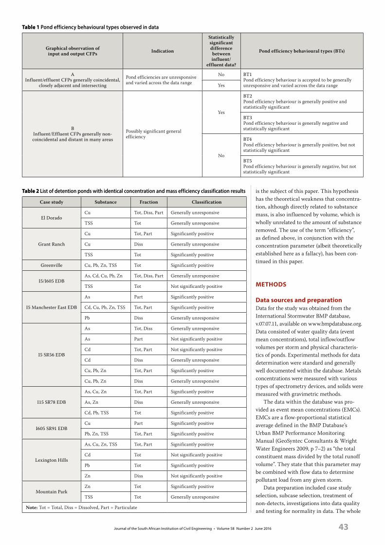
Journal of the South African Institution of Civil Engineering • Volume 58 Number 2 June 2016 43
is the subject of this paper. This hypothesis has the theoretical weakness that concentra-tion, although directly related to substance mass, is also influenced by volume, which is wholly unrelated to the amount of substance removed. The use of the term “efficiency”, as defined above, in conjunction with the concentration parameter (albeit theoretically established here as a fallacy), has been con-tinued in this paper.
MethodS
data sources and preparationData for the study was obtained from the International Stormwater BMP database, v.07.07.11, available on www.bmpdatabase.org. Data consisted of water quality data (event mean concentrations), total inflow/outflow volumes per storm and physical characteris-tics of ponds. Experimental methods for data determination were standard and generally well documented within the database. Metals concentrations were measured with various types of spectrometry devices, and solids were measured with gravimetric methods.
The data within the database was pro-vided as event mean concentrations (EMCs). EMCs are a flow-proportional statistical average defined in the BMP Database’s Urban BMP Performance Monitoring Manual (GeoSyntec Consultants & Wright Water Engineers 2009, p 7–2) as “the total constituent mass divided by the total runoff volume”. They state that this parameter may be combined with flow data to determine pollutant load from any given storm.
Data preparation included case study selection, subcase selection, treatment of non-detects, investigations into data quality and testing for normality in data. The whole
Table 1 Pond efficiency behavioural types observed in data
Graphical observation of input and output CFPs Indication
Statistically significant difference between influent/
effluent data?
Pond efficiency behavioural types (BTs)
AInfluent/effluent CFPs generally coincidental,
closely adjacent and intersecting
Pond efficiencies are unresponsive and varied across the data range
No BT1Pond efficiency behaviour is accepted to be generally unresponsive and varied across the data rangeYes
BInfluent/Effluent CFPs generally non-coincidental and distant in many areas
Possibly significant general efficiency
Yes
BT2Pond efficiency behaviour is generally positive and statistically significant
BT3Pond efficiency behaviour is generally negative and statistically significant
No
BT4Pond efficiency behaviour is generally positive, but not statistically significant
BT5Pond efficiency behaviour is generally negative, but not statistically significant
Table 2 List of detention ponds with identical concentration and mass efficiency classification results
Case study Substance Fraction Classification
El DoradoCu Tot, Diss, Part Generally unresponsive
TSS Tot Generally unresponsive
Grant Ranch
Cu Tot, Part Significantly positive
Cu Diss Generally unresponsive
TSS Tot Significantly positive
Greenville Cu, Pb, Zn, TSS Tot Significantly positive
I5/I605 EDBAs, Cd, Cu, Pb, Zn Tot, Diss, Part Generally unresponsive
TSS Tot Not significantly positive
I5 Manchester East EDB
As Part Significantly positive
Cd, Cu, Pb, Zn, TSS Tot, Part Significantly positive
Pb Diss Generally unresponsive
I5 SR56 EDB
As Tot, Diss Generally unresponsive
As Part Not significantly positive
Cd Tot, Part Not significantly positive
Cd Diss Generally unresponsive
Cu, Pb, Zn Tot, Part Significantly positive
Cu, Pb, Zn Diss Generally unresponsive
I15 SR78 EDB
As, Cu, Zn Tot, Part Significantly positive
As, Zn Diss Generally unresponsive
Cd, Pb, TSS Tot Significantly positive
I605 SR91 EDBCu Part Significantly positive
Pb, Zn, TSS Tot, Part Significantly positive
Lexington Hills
As, Cu, Zn, TSS Tot, Part Significantly positive
Cd Tot Not significantly positive
Pb Tot Significantly positive
Zn Diss Not significantly positive
Mountain ParkZn Tot Significantly positive
TSS Tot Generally unresponsive
Note: Tot = Total, Diss = Dissolved, Part = Particulate

Journal of the South African Institution of Civil Engineering • Volume 58 Number 2 June 201644
project consisted of investigations into 10 detention pond and 20 retention pond case studies. Data was divided into a total of 120 metals and solids subcases, namely arsenic, cadmium, copper, lead, zinc, total suspended solids (TSS) and total volatile solids (TVS). Further division of subcases into total and dissolved fractions yielded 168 data sets.
The Regression on Order Statistics (ROS) method was used to estimate non-detect (censored) values for statistical calculations. The software application NADA for R ver-sion 2.15.0 (The R Foundation for Statistical Computing, copyright 2012) was used to model values. Mass data was calculated from ROS modelled non-detect values only in cases where the position of the modelled value in relation to volume data was clear, i.e. where there was no doubt that the modelled value related to a specific storm event. Data sets with > 80% non-detects could not be modelled (Helsel & Lee 2005) and were left unchanged.
Quality assurance: data reviewsData was deleted from raw datasets in the following cases:1. Paired datasets where the measured solu-
ble concentration was reported to be a value larger than the measured total con-centration. It was impossible to ascertain where the error occurred, and therefore total and soluble data in such cases were wholly removed from the datasets.
2. Datasets where the non-detects were reported with a method detection limit that was higher than any of the measured data. This scenario does not allow for any insight into the placement of data on a ranking scale; it only shows that the non-detects are somewhere within the whole range of the measured data. Such non-detect data was therefore deleted from the datasets.
3. Data that had been identified in the database by the data providers as “not for further use in water quality or volumetric analyses”.
4. Data coded as grab samples. The majority of data comprised event-mean concentra-tions. Grab samples could not be assumed to represent mean concentrations and were therefore not included in further data analyses.
StatisticsDescriptive statistics were calculated with the software program STATISTICA v.10 (Copyright© StatSoft Inc 1984–2011). The results of normality testing indicated a lack of normality in a great number of datasets (untransformed as well as log-transformed). Non-parametric descriptive statistics
Table 3 List of retention ponds with identical concentration and mass efficiency classification results
Case study Substance Fraction Classification
Central Park Pb, Zn Tot Significantly positive
Cockroach BayPb Tot Not significantly negative
TSS Tot Not significantly positive
De Bary
Cu Part Generally unresponsive
Pb Tot Not significantly positive
Zn Tot, Diss Significantly positive
Zn Part Not significantly positive
TSS Tot Significantly positive
Greens Bayou
Cu Diss Not significantly negative
Pb Tot Not significantly negative
Zn Part Not significantly negative
Heritage Estates
Cd Tot Generally unresponsive
Cu Tot Significantly positive
Pb, Zn, TSS Tot Not significantly positive
I5 La Costa East
Cd, Cu, Pb, Zn, TSS Tot, Part Significantly positive
Cu, Zn Diss Not significantly positive
Pb Diss Significantly positive
Lake Ellyn
Cu, Pb, Zn, TSS Tot, Part Significantly positive
Pb Diss Significantly negative
Zn Diss Significantly positive
Lake Ridge Pb, TSS, TVS Tot Significantly positive
Madison Monroe StPb Tot Not significantly positive
TSS, TVS Tot Significantly positive
McKnight Basin Pb, TSS, TVS Tot Significantly positive
Phantom Lake Pond A Cu, Pb, Zn, TSS Tot Significantly positive
PinellasCu Tot Significantly positive
TSS, TVS Tot Generally unresponsive
PittsfieldPb Tot Not significantly positive
TSS Tot Significantly positive
Runaway Bay Zn, TSS Tot Not significantly positive
Silver Star Rd
Pb, Zn Tot Generally unresponsive
Pb Diss Significantly positive
Pb Part Significantly negative
Zn Diss, Part Generally unresponsive
TSS, TVS Tot Significantly negative
Tampa Office Pond 1 Zn Tot Significantly positive
Tampa Office Pond 2Cd, Zn Tot Not significantly positive
TSS Tot Significantly positive
Tampa Office Pond 3 Pb, Zn, TSS Tot Significantly positive
University of New Hampshire Zn Tot Significantly positive
Note: Tot = Total, Diss = Dissolved, Part = Particulate

Journal of the South African Institution of Civil Engineering • Volume 58 Number 2 June 2016 45
were therefore further used to determine measures of location, central tendency and spread. The results of these analyses were not directly pertinent to the arguments pre-sented in this paper and were therefore not explicitly included.
the effluent Probability Method (ePM)The EPM provides a statistical view of influent and effluent quality, and has been recommended by GeoSyntec Consultants & Wright Water Engineers (2009) under sup-port from inter alia the Water Environment Research Foundation (WERF), the United States Environmental Protection Agency (USEPA) and the American Society of Civil Engineers (ASCE).
The methodology broadly comprises the following steps:1. Determine whether a BMP is providing
treatment by calculating statistical sig-nificance at 95% confidence level between influent and effluent values.
2. Examine a cumulative distribution func-tion or standard parallel probability plot of influent and effluent quality. (GeoSyntec Consultants & Wright Water Engineers 2009)
The results of the statistical analysis indi-cated that normality could not be assumed in many datasets and that difference values between influent and effluent data were non-symmetrical. The state of the data therefore necessitated the use of the non-parametric, but less powerful, Sign test for testing of sta-tistical significance. The software program STATISTICA v.10 (Copyright© StatSoft Inc 1984–2011) was used for all calculations of statistical significance. Statistical signifi-cance between influent and effluent data was accepted at p < 0.05. A table published by Dixon (1953, Table 1, p 468) was used to estimate power.
Cumulative Distribution Functions (CDFs) can be approximated by Cumulative Frequency Plots (CFPs) and can be displayed on these plots to determine how well the data fits a theoretical (e.g. normal) distribu-tion (GeoSyntec Consultants & Wright Water Engineers 2009). However, the estab-lishment of pond efficiencies for comparative purposes did not require the establishment of theoretical distributions. Normality of datasets was established through the use of Normal Probability Plots in order to inform the choice between statistical tests. Therefore, the sample approximations of the CDFs, i.e. CFPs, were deemed adequate for the graphical representations of data in this project.
STATISTICA v.10 (Copyright© StatSoft Inc 1984–2011) was used to generate CFPs.
Table 4 List of detention ponds with contradictory concentration/mass efficiency classification results
Case study Substance Fraction Classification – Concentration Classification – Mass Strength
of result
I5 Manchester East EDB
As Tot Generally unresponsive Significantly positive Informative
As Diss Not significantly negative Not significantly positive Informative
Cd Diss Not significantly positive Generally unresponsive Arguable
Cu Diss Generally unresponsive Significantly positive Informative
Zn Diss Generally unresponsive Significantly positive Informative
I5 SR56 EDB TSS Tot Significantly positive Not significantly positive Arguable
I15 SR78 EDB Cu Diss Generally unresponsive Significantly positive Informative
I605 SR91 EDB
Cu Tot Not significantly positive Significantly positive Arguable
Cu Diss Not significantly negative Significantly positive Informative
Pb Diss Generally unresponsive Significantly positive Informative
Zn Diss Not significantly positive Significantly positive Arguable
Lexington Hills
As Diss Generally unresponsive Not significantly positive Arguable
Cu Diss Not significantly negative Not significantly positive Informative
Note: Tot = Total, Diss = Dissolved, Part = Particulate
Table 5 List of retention ponds with contradictory concentration and mass efficiency classification results
Case study Substance Fraction Classification – Concentration Classification – Mass Strength
of result
Central Park
Cd Tot Significantly positive Significantly negative Informative
Cu, TSS, TVS Tot Significantly positive Not significantly positive Arguable
Cockroach Bay Cu Tot Not significantly positive Significantly positive Arguable
De Bary Cu Tot, Diss Significantly positive Generally unresponsive Informative
Greens Bayou
Cu Tot, Part Not significantly negative Generally unresponsive Arguable
Zn Tot, Diss Significantly negative Not significantly
negative Arguable
TSS Tot Significantly positive Not significantly positive Arguable
I5 La Costa East Cd Diss Not significantly positive Generally unresponsive Arguable
Lake Ellyn Cu Diss Significantly positive Generally unresponsive Informative
Lakeside Zn, TSS Tot Significantly positive Not significantly positive Arguable
PinellasPb Tot Significantly positive Generally unresponsive Informative
Zn Tot Significantly positive Not significantly positive Arguable
Tampa Office Pond 1
TSS Tot Significantly positive Not significantly positive Arguable
Tampa Office Pond 2
Cu Tot Generally unresponsive Not significantly positive Arguable
Tampa Office Pond 3
Cd, Cu Tot Significantly positive Not significantly positive Arguable
University of New Hampshire
TSS Tot Significantly positive Not significantly positive Arguable
Note: Tot = Total, Diss = Dissolved, Part = Particulate

Journal of the South African Institution of Civil Engineering • Volume 58 Number 2 June 201646
The Lowess smoothing method was used in the generation of regression lines, while graphical observations were limited to visual categorisation of graphical behaviour according to plot point and regression line proximity.
classification of pond efficienciesRelationships between input and output CFPs resulted in the classification of general pond efficiencies into two different obser-vational types. Additional consideration of statistical significance results led to the establishment of five different behavioural types (BTs), which are discussed further below. The criteria for the selection of BTs are shown in Table 1 (p 43).
reSultS ANd dIScuSSIoN
dataset efficiency classificationsPond efficiencies were classified separately for substance type (metals and solids), as well as fraction (total, dissolved or particulate). Tables 2 to 5 (pp 43–45) contain lists of detention and retention ponds with similar and dissimilar concentration and mass effi-ciency classification results.
The power of the Sign test results was low for the majority of detention and reten-tion pond total (concentration and mass) cases where statistical significance between influent and effluent values was not found. It is therefore possible that, due to effect size, these case studies may have produced signifi-cant results if larger sample sizes had been available. However, the subject of this inves-tigation was to ascertain if concentration and mass data provide similar interpretations of efficiency with the EPM. Therefore, the focus was on the data at hand, and hypotheses regarding different outcomes with larger data samples were considered to be irrelevant.
Classifications where subjectivity may have resulted in arguable outcomes, namely classifications labelled as “not significantly positive”, “not significantly negative” or “gen-erally unresponsive” were found in a number of cases. Efficiency classifications of such cases may have been found to be identical rather than contradictory if (1) more data had been available to improve the power and change the outcome of the statistical significance results, or (2) a different (and subjective) decision regarding the graphical display of data had been made.
Therefore it is possible that, under differ-ent circumstances, similar concentration and mass classifications may have been found for cases where the classifications were combi-nations of (1) not significantly positive and significantly positive, (2) not significantly
negative and significantly negative, and (3) not significantly positive/negative and generally unresponsive. In this research such cases include the following: I5 Manchester East EDB (dissolved cadmium), I5 SR56 EDB (TSS), I605 SR91 EDB (total copper, dissolved
zinc), Lexington Hills Pond (dissolved arse-nic), Central Park Pond (total copper, TSS, TVS), Cockroach Bay Pond (total copper), Greens Bayou (total and particulate copper, total and dissolved zinc, TSS), I5 La Costa East EDB (dissolved cadmium), Lakeside
Figure 1 I5 Manchester East EDB CFP for arsenic concentration influent/effluent values
Frac
tion
of v
alue
s bel
ow
1.00
0.60
0.40
0.20
Concentration (μg/l)0.250 1.8 2.6 3.0
Histogram of multiple variables
0.80
00.8 1.0 2.21.5
Tot_In Tot_Out Diss_In Diss_Out Part_In Part_Out
Appendix*: CFP's for Detention Ponds - As
Figure 2 I5 Manchester East EDB CFP for arsenic mass influent/effluent values
Frac
tion
of v
alue
s bel
ow
1.00
0.60
0.40
0.20
Mass (g)
0.01
3
Histogram of multiple variables
0.80
0
Tot_In Tot_Out Diss_In Diss_Out Part_In Part_Out
0.03
8
0.05
60.
066
0.08
70.
104
0.12
3
0.15
6
0.22
1
0.47
4
0.66
2
Appendix*: CFP's for Detention Ponds - As
0.01
3
0.03
8
0.05
60.
066
0.08
70.
104
0.12
30.
156
0.22
1
0.47
4
0.66
2
Mass, g

Journal of the South African Institution of Civil Engineering • Volume 58 Number 2 June 2016 47
Pond (total zinc, TSS), Pinellas Pond (total zinc), Tampa Office Pond 1 (TSS), Tampa Office Pond 2 (total copper), Tampa Office Pond 3 (total cadmium, total copper) and University of New Hampshire Pond (TSS).
Cases where the differences between influent and effluent values were statistically significant, combined with CFPs that were obviously distant, classifications such as
“significantly positive” or “significantly nega-tive” are well founded and not considered to be arguable. Therefore, cases where the concentration and mass classifications were combinations – (1) positive and negative, or (2) generally unresponsive and significantly positive/negative – they have notable differ-ences between concentration and mass effi-ciencies. Such cases included the following:
I5 Manchester East EDB (total and dissolved arsenic, dissolved copper, dissolved zinc), I15 SR78 EDB (dissolved copper), I605 SR91 EDB (dissolved copper, dissolved lead), Lexington Hills (dissolved copper), Central Park Pond (total cadmium), De Bary Pond (total and dissolved copper), Lake Ellyn (dissolved cop-per) and the Pinellas Pond (total lead).
No evidence was found to suggest that contradictory concentration/mass classifica-tions may be linked to specific substances. Contradictory results for both detention and retention ponds encompassed all metals (arsenic, cadmium, copper, lead, zinc) and solids subcases (TSS, TVS).
Graphical data behaviourInvestigation of CFPs showed differences in concentration and mass data behaviour that were obscured by the simplistic singular effi-ciency classification results. Two informative cases were selected for illustrative purposes (see Figures 1 to 4).
The I5 Manchester East EDB (arsenic) CFPs indicate markedly different total and dissolved arsenic concentration and mass efficiencies. Total concentration influent/effluent data behaviour is closely adjacent along the majority of the data range while, in contrast, total mass influent/effluent data is distant along the majority of the data range. Dissolved concentration influent/effluent CFPs indicate negative removals along the majority of the data range while, in contrast, the mass influent/effluent CFPs indicate positive removals along the majority of the data range. Interpretation of the concentra-tion graphs therefore leads to an inference of poor total and negative dissolved pond efficiencies, while the interpretation of the mass data indicates considerably better and generally positive pond efficiencies.
The Central Park Pond CFPs (total cadmium) indicate positive concentration efficiencies and negative mass efficiencies. Therefore, interpretation of the concentra-tion graph leads to an inference of positive total pond efficiencies, while the interpreta-tion of the mass data indicates much poorer negative efficiencies.
These graphs illustrate erroneous con-clusions that can be made regarding pond efficiencies through the use of concentration as a parameter for the determination of the amount of substance removed, namely:1. In the I5 Manchester East EDB it is
possible that physical pond functioning influenced influent arsenic concentra-tions in such a way that substances were more concentrated when they reached the pond effluent stream. This does not mean that the pond did not remove substances, as was evidenced by the mass data, only
Figure 3 Central Park Pond CFPs for total cadmium concentration influent/effluent values
Frac
tion
of v
alue
s bel
ow
1.00
0.60
0.40
0.20
Concentration (μg/l)0.1 0.8
0.80
00.4
Tot_In Tot_Out
Figure 4 Central Park Pond CFPs for total cadmium mass influent/effluent values
Frac
tion
of v
alue
s bel
ow
1.00
0.60
0.40
0.20
Mass (g)0.1 3.0
0.80
00.7
Tot_In Tot_Out

Journal of the South African Institution of Civil Engineering • Volume 58 Number 2 June 201648
that the substances became more concen-trated within the pond.
2. The Central Park pond sources of influ-ent other than the influent stream, such as direct overland flow, direct rainfall or base flow, may have increased pond volumes and decreased influent cadmium concentrations, thereby reducing efflu-ent concentrations. This does not mean that the pond removed cadmium, as was evidenced by the mass data, only that the substance became less concentrated within the pond.
coNcluSIoNSThe subject of this paper was an inves-tigation into the hypothesis that the concentration parameter may be used as a proxy parameter for mass in the Effluent Probability Method (EPM) to ascertain the amount of substance removed by a structure, i.e. its efficiency. The results of theoretical considerations and data analyses negate this hypothesis. Theoretically, the hypothesis has the weakness that concentration, although mathematically directly related to mass, is also influenced by volume, which is com-pletely unrelated to mass.
Data investigations showed that many of the resultant contradictory classifications for concentration and mass data may be arguable. Different graphical interpretations may have resulted in similar classifications for concen-tration and mass data in some cases. However, a noteworthy number of cases had contradic-tory concentration and mass classifications that were not deemed to be fundamentally arguable. Cases wherein (1) concentration and mass removals were opposite (i.e. positive and negative), or (2) where significant removals were found for concentration, and generally
unresponsive behaviour was seen for mass (and vice versa), were deemed to have unargu-ably contradictory concentration and mass data behaviours.
Therefore, the efficiency classification results (Tables 2–5 on pp 43–45) indicate that different classifications were possible for evaluations of concentration and mass efficiencies. Such differences were due to different concentration and mass data behaviours, as illustrated in Figures 1 and 2. Pond influent concentrations changed within ponds with subsequent increases or decreases in effluent concentration values without con-current increases or decreases in mass values.
Figures 1 and 2 demonstrate erroneous conclusions that can be made through the use of the concentration parameter, namely (1) increases in effluent concentrations compared to influent concentrations do not necessarily mean that the pond did not remove substances, only that the substances became more concentrated within the pond, and (2) decreases in effluent concentrations compared to influent concentrations do not necessarily mean that the pond removed substances, only that the substances became less concentrated within the pond.
Therefore the results suggest that not only is the use of the concentration parame-ter as a proxy parameter for mass unfounded for use in the EPM, but, in addition, errone-ous conclusions regarding pond efficiencies can be made. It is therefore recommended that the mass parameter be used for determi-nation of pond efficiencies with the EPM.
refereNceSBarrett, M E 2008. Comparison of BMP performance
using the international BMP database. Journal of
Irrigation and Drainage Engineering, 134(5): 556–561.
Chen, C F, Lin, J Y, Huang, C H, Chen, W L &
Chueh, N L 2009. Performance evaluation of full-
scale natural treatment system for nonpoint source
and point source pollution removal. Environmental
Monitoring and Assessment, 157(1): 391–406.
Dixon, W J 1953. Power functions of the sign test and
power efficiency for normal alternatives. Annals of
Mathematical Statistics, 24(3): 467–473. Available
at: http://www.jstor.org (accessed on 29 September
2011).
Fassman, E 2012. Stormwater BMP treatment
performance variability for sediment and heavy
metals. Separation and Purification Technology,
84: 95–103.
GeoSyntec Consultants & Wright Water Engineers
2009. Urban stormwater BMP performance
monitoring. Available at: http://www.bmpdatabase.
org (accessed on 17 May 2011).
Geosyntech Consultants Inc & Wright Water
Engineers Inc 2011. International stormwater Best
Management Practices (BMP) database. Pollutant
category summary: Metals. Available at: http://www.
bmpdatabase.org (accessed on 28 September 2011).
Greb, S R & Bannerman, R T 1997. Influence of particle
size on wet pond effectiveness. Water Environment
Research, 69(6): 1134–1138.
Helsel, D R & Lee, L 2005. Statistical analysis of
water-quality data containing multiple detection
limits: S-language software for regression on
order statistics. Computers & Geosciences, 31(10):
1241–1248.
Hossain, M A, Alam, M, Yonge, D R & Dutta, P 2005.
Efficiency and flow regime of a highway stormwater
detention pond in Washington, USA. Water, Air, and
Soil Pollution, 164(1): 79–89.
Strecker, E W, Quigley, M M, Urbonas, B R, Jones, J E &
Clary, J K 2001. Determining urban stormwater BMP
effectiveness. Journal of Water Resources Planning
and Management, 127(3): 144–149.

49Brink IC, Kamish W. Stormwater pond metals and solids removal efficiency determination with the effluent probability method: A novel classification system. J. S. Afr. Inst. Civ. Eng. 2016;58(2), Art. #TN-69, 7 pages. http://dx.doi.org/10.17159/2309-8775/2016/v58n2a6
techNIcAl NoteJournal of the South african inStitution of civil engineeringVol 58 No 2, June 2016, Pages 49–55, Technical Note 69
ISOBEL BRInK (Associate Member SAICE) is a PhD student in Civil Engineering at Stellenbosch University. She obtained a B Bldg Arts degree from the University of Port Elizabeth in 1999, and a BSc and an MSc in Civil Engineering from the University of Cape Town in 2005 and 2008 respectively (with her MSc specialising in water quality). She was on the Dean’s Merit List for all
her civil engineering undergraduate study years, which she completed with first-class honours.
Contact details: Department of Civil Engineering Stellenbosch University Private Bag X1 Matieland, 7602 South Africa T: +27 21 808 4195 E: [email protected]
WAGEED KAMISH (Pr Eng) obtained a BSc in Chemical Engineering from the University of Cape Town and an MSc in Civil Engineering from Stellenbosch University, where he is also completing his PhD studies in Environmental Engineering. He has 18 years’ experience in the water quality field and has specifically been focusing on water quality situation assessments
for water resource studies, as well as hydrodynamic water quality and hydrological modelling. More recently he has been involved in cleaner production projects and computational fluid dynamics analyses in support of bulk infrastructure designs.
Contact details: Department of Civil Engineering Stellenbosch University Private Bag X1 Matieland, 7602 South Africa T: +27 21 808 4352 E: [email protected]
Keywords: standard classification system, stormwater pond, metals removal
INtroductIoNThis technical note presents information on the development and application of a classifi-cation system for use as a supplement to the Effluent Probability Method (EPM). It is part of a larger project into the determination of links between stormwater pond efficiency, in terms of metals and solids removal, and design. It became apparent during the course of the project that a scheme that enabled the comparison of case studies in terms of efficiency was required. A literature search yielded no such system, necessitating the development of the classification system presented here.
The definition of stormwater pond effi-ciency used in this paper was adopted from literature provided by the United States of America Environmental Protection Agency (USEPA) and reads as follows: “Efficiency is a measure of how well a BMP (read Best Management Practice) or BMP system removes pollutants” (Geosyntech Consultants et al 1999). In this paper, the term “efficiency” refers specifically to how well a stormwater pond removes metals and solids.
The Effluent Probability Method (EPM) has been used in a number of studies to determine stormwater structure substance removal efficiencies, e.g. Chen et al (2009), Geosyntech Consultants Inc & Wright Water Engineers Inc (2011), and Fassman (2012). The findings of Chen et al (2009) and Geosyntech Consultants Inc & Wright Water Engineers Inc (2011) are limited to graphical comparisons of influent and effluent data for specific substances with cumulative frequency plots. The findings
of Fassman (2012) are limited to categorical (swales, wetlands, etc) graphical com-parisons of substance effluent event mean concentrations.
These studies illuminate a shortcom-ing of the EPM, namely that efficiency of specific structures can only be subjectively quoted, simply as “more or less efficient” in relation to other structures, with no scheme to suggest how “efficient” or “inefficient” a structure is.
the efflueNt ProbAbIlIty MethodThe EPM provides a statistical view of influent and effluent quality and was recom-mended by GeoSyntec Consultants & Wright Water Engineers (2009) under support from inter alia the Water Environment Research Foundation (WERF), the United States Environmental Protection Agency (USEPA) and the American Society of Civil Engineers (ASCE).
This methodology broadly comprises the following steps:1. Determine whether a BMP is providing
treatment by calculating statistical sig-nificance at 95% confidence level between influent and effluent values.
2. Examine a cumulative distribution func-tion or standard parallel probability plot of influent and effluent quality. (GeoSyntec Consultants & Wright Water Engineers 2009)
The advantages of the EPM are: (1) it is easy to apply, and (2) it provides a clear picture of the effluent vs influent water quality.
Stormwater pond metals and solids removal efficiency determination with the effluent probability method: A novel classification systemI C Brink, W Kamish
This technical note contains findings from a larger research project into the design of stormwater detention and retention ponds for removal of metals and solids. The project required a standard system with which case studies obtained from the International Stormwater BMP Database could be compared in terms of efficiency. A novel classification system for use with the Effluent Probability Method, designed for this purpose, was developed and is presented here.

Journal of the South African Institution of Civil Engineering • Volume 58 Number 2 June 201650
Shortcomings of the method are:1. The measure of statistical significance
is only a measure that proves/disproves the null hypothesis that the influent and effluent data medians are equal at a pre-defined significance level. It cannot prove that influent concentration has some impact on effluent concentration.
2. Graphical displays of data provide only a sense of pond performance. Personal judgement must be used to conclude whether a pond performs well or poorly in relation to other ponds.
Cumulative distribution functions (CDFs) can be approximated by cumulative fre-quency plots (CFPs) (GeoSyntec Consultants & Wright Water Engineers 2009). CFPs are variations of histograms, in which the height of each bar represents the total number of observations that are less than or equal to the upper limit of the bin (Montgomery & Runger 2003). These graphs are useful in pond efficiency evaluations, because they can indicate variations in pond efficiencies over inflow/outflow data ranges. The establish-ment of pond efficiencies for comparative purposes in this project did not require the establishment of theoretical distributions. Normality of datasets was established through the use of normal probability plots in order to inform the choice between statis-tical tests. Therefore, the sample approxima-tions of the cumulative distribution func-tions, i.e. CFPs, were deemed adequate for the graphical representations of data.
The use of statistical significance is con-troversial and has been criticised. Dickson and Baird (2011) stated that, although statistical significance testing has become the standard in many scientific explorations, the assumption that a significant differ-ence is due to some causal relationship is
Table 1 Pond efficiency behavioural types observed in data
Graphical observation Indication
Statistically significant difference between inflow/
outflow data?
Pond efficiency behavioural types (BT)
AIn/out CFPs generally coincidental,
closely adjacent and intersecting
Pond efficiencies are unresponsive and varied across the data range
Yes BT1Pond efficiency behaviour is accepted to be generally unresponsive and varied across the data rangeNo
BCFPs generally non-coincidental
and distant in many areas
Possibly significant general efficiency
Yes
BT2Pond efficiency behaviour is generally positive and statistically significant
BT3Pond efficiency behaviour is generally negative and statistically significant
No
BT4Pond efficiency behaviour is generally positive, but not statistically significant
BT5Pond efficiency behaviour is generally negative, but not statistically significant
Table 2 Sign test p-value results for selected case studies
Case study
Sign test p-value
Total Dissolved Particulate
Conc Mass Conc Mass Conc Mass
I5/I605 EDB – zinc 0.15 0.15 0.009 0.009 0.77 0.77
Lake Ellyn – zinc 0.00006 0.00006 0.00006 0.002 0.0004 0.0004
I605 SR91 EDB – copper 0.22 0.04 0.68 0.04 0.04 0.04
Central Park – cadmium 0.03 0.01 no data no data no data no data
Note: Values in bold denote statistically significant results at p < 0.05.Values in italics denote results with low statistical power (< 0.8).
Figure 1 I5 I605 EDB CFPs for zinc concentration inflow/outflow values
Frac
tion
of v
alue
s bel
ow
1.00
0.60
0.40
0.20
Concentration (μg/l)
1.40
0
0.80
0
Tot_In Tot_Out Diss_In Diss_Out Part_In Part_Out
24.0
00
77.0
0091
.300
108.
000
130.
000
219.
000
361.
000
15.0
00
40.0
0044
.400
52.2
0059
.000
65.0
00

Journal of the South African Institution of Civil Engineering • Volume 58 Number 2 June 2016 51
currently “more an article of faith than a well-established principle”. On the choice of the significance level, Dickson & Baird (2011) stated that the choice of significance
level is in itself statistically insignificant, is arbitrary and unbased in theory. Statistical significance should therefore be used with cognisance of the criticisms raised against
it. The EPM reduces the chance of draw-ing incorrect conclusions from the p-value by coupling its interpretation with that of graphical displays of data.
clASSIfIcAtIoN SySteM develoPMeNt
Statistical significance testingData was obtained from the International Stormwater BMP Database, v.07.07.11, avail-able on www.bmpdatabase.org. Normality test results indicated that normality could not be assumed in many datasets, and that difference values between inflow and outflow data were generally non-symmetrical. The Sign test was therefore chosen for use. It has been con-sidered by Dixon and Mood (1946) to be most useful when (1) there are pairs of observations on the two things being compared, (2) each of the two observations of a given pair arose under similar conditions, and (3) the dif-ferent pairs were observed under different conditions. This condition generally makes the t-test invalid. These conditions were suited for use with the data of this project where (1) pond inflow and outflow data could be seen as pairs, (2) the inflow and outflow data arose under the same storm and runoff conditions, and (3) different storm inflow and outflow data pairs arose under different storms and different runoff conditions.
The software program STATISTICA v.10 (Copyright© StatSoft Inc 1984–2011) was used for all calculations. Statistical signifi-cance between inflow and outflow data was accepted at p < 0.05. A table published by Dixon (1953) (Table 1, p 468) was used to estimate power.
cumulative frequency Plots (cfPs)Graphical observations were limited to visual categorisation of graphical behaviour according to plot point and regression line proximity. STATISTICA v.10 (Copyright© StatSoft Inc 1984–2011) was used to generate CFPs for all datasets. The Lowess smooth-ing method was used for the generation of regression lines.
classification of pond efficienciesRelationships between in/out CFPs resulted in the categorisation of general pond effi-ciencies into two basic observational types. Additional consideration of statistical signifi-cance results led to the establishment of five different behavioural types (BTs), shown in Table 1.
The behavioural types of pond efficien-cies were classified as follows:1. BT1 – Generally unresponsive efficien-
cy: Pond efficiencies were classified as
Figure 2 I5 I605 EDB CFPs for zinc mass inflow/outflow values
Frac
tion
of v
alue
s bel
ow
1.00
0.60
0.40
0.20
0.18
9
0.80
0
Mass (g)Tot_In Tot_Out Diss_In Diss_Out Part_In Part_Out
1.63
5
2.83
3
3.99
5
5.91
8
8.71
310
.285
14.5
69
20.6
4127
.006
38.9
37
59.2
9378
.854
124.
989
200.
684
0.18
9
1.63
5
2.83
33.
995
5.91
8
8.71
310
.285
14.5
6920
.641
27.0
0638
.937
59.2
9378
.854
124.
989
200.
684
Mass, g
Figure 3 Lake Ellyn CFPs for zinc concentration inflow/outflow values
Frac
tion
of v
alue
s bel
ow
1.00
0.60
0.40
0.20
Concentration (μg/l)
3.00
0
0.80
0
Tot_In Tot_Out Diss_In Diss_Out Part_In Part_Out
Histogram of multiple variables
5.39
66.
090
8.73
4
11.3
1813
.091
17.1
2320
.052
23.1
6425
.863
30.8
4538
.692
46.0
0055
.450
80.0
00
153.
000
200.
000
240.
000
320.
000
593.
400

Journal of the South African Institution of Civil Engineering • Volume 58 Number 2 June 201652
generally unresponsive in cases where in/out data points and regression lines in the CFPs were coincidental, closely adjacent and/or intersected along the majority of the data range. A statistically significant result for the dataset was not held to negate this classification. This is because the Sign test results indicated significant differences (below a certain arbitrarily chosen p-value) between medians and could not prove or disprove efficiency on its own. Therefore, visual interpretation of graphical displays of data trumped the results of the Sign test in this case.
2. BT2 – Significantly positive efficiency: Pond efficiencies were classified as significantly positive when (a) in/out data points and regression lines on the CFPs were generally positive, non-coincidental and distant in the majority of the data range, and (b) the Sign test gave a statisti-cally significant result for paired inflow and outflow datasets.
3. BT3 – Significantly negative efficiency: Pond efficiencies were classified as sig-nificantly negative when: (a) in/out data points and regression lines on the CFPs were generally negative, non-coincidental and distant in the majority of the data range, and (b) the Sign test gave a statisti-cally significant result for paired inflow and outflow datasets.
4. BT4 – Not significantly positive effi-ciency: Pond efficiencies were classified as not significantly positive when: (a) in/out data points and regression lines on the CFPs were generally positive, non-coincidental and distant in the majority of the data range, and (b) the Sign test did not give a statistically significant result for paired inflow and outflow datasets.
5. BT5 – Not significantly negative effi-ciency: Pond efficiencies were classified as not significantly negative when: (a) in/out data points and regression lines on the CFPs were generally negative, non-coincidental and distant in the majority of the data range, and (b) the Sign test did not give a statistically significant result for paired inflow and outflow datasets.
eXAMPleSThe results of four case studies are presented to provide examples to illustrate the use of the classification system. Examples were specifically chosen to illustrate the different classification types.
Sign test resultsP-values for the selected case studies are shown in Table 2 (p 50). Results were deemed to be statistically significant at p < 0.05.
The power of the sign test was low (< 0.8) for (1) the I5/I605 EDB total and particulate zinc concentration and mass, and (2) the I605 SR91 EDB total and dissolved copper
concentration datasets. The power of the Sign test can be greatly influenced by sample size (see Dixon 1953) and it is therefore pos-sible that these cases might have produced
Figure 4 Lake Ellyn CFPs for zinc mass inflow/outflow values
Frac
tion
of v
alue
s bel
ow
1.00
0.60
0.40
0.20
Mass (g)
8.45
3
0.80
0
Tot_In Tot_Out Diss_In Diss_Out Part_In Part_Out
Histogram of multiple variables
27.6
94
55.7
6274
.318
86.9
3610
6.18
813
2.30
515
3.02
117
6.47
122
8.22
429
6.56
237
2.62
148
3.79
354
2.06
965
5.81
876
9.55
092
6.13
11
056.
926
1 29
5.49
6
2 22
9.78
12
732.
575
Figure 5 I605 SR91 EDB CFPs for copper concentration inflow/outflow values
Frac
tion
of v
alue
s bel
ow
1.00
0.60
0.40
0.20
Concentration (μg/l)4.00
0.80
0
Tot_In Tot_Out Diss_In Diss_Out Part_In Part_Out
Histogram of multiple variables
10.30 14.50 20.00 24.30 37.00

Journal of the South African Institution of Civil Engineering • Volume 58 Number 2 June 2016 53
statistically significant results if larger sample sizes had been available.
Graphical displays of dataCFPs for the selected case studies are pro-vided in Figures 1–8. The following terms were used in the graphs:
■ Tot_In: Total substance in inflow ■ Tot_Out: Total substance in outflow ■ Diss_In: Dissolved substance in inflow ■ Diss_Out: Dissolved substance in outflow ■ Part_In: Particulate substance in inflow ■ Part_Out: Particulate substance in
outflow
observations and efficiency classificationsBehavioural observations coupled with the Sign test results and the resultant efficiency classifi-cations are summarised in Table 3 (p 54).
AdvANtAGeS of the clASSIfIcAtIoN SySteM1. It provides a standardised methodology,
as well as terminology for pond efficiency classification through the creation of a singular descriptor of pond efficiencies, which can be used as a quick reference for comparison across case studies.
2. It is a supplement to the EPM, which is a highly recommended method (see GeoSyntec Consultants & Wright Water Engineers 2009) for pond efficiency determinations. The basis of the method is therefore already well established amongst stormwater quality researchers.
ShortcoMINGS of the clASSIfIcAtIoN SySteM1. An advantage of the system, namely the
provision of a singular descriptor of pond efficiency, is also a disadvantage. From the results it can be seen that complex cases may arise in which classification is overly simplified, resulting in failure to highlight underlying and complicated pond behaviour. For example, the I5 I605 EDB total zinc removal efficiencies for concentration and mass were classified as “generally unresponsive”. Closer inspec-tion of the CFPs showed that removals were positive at higher values and nega-tive at lower values, and this behavioural inconsistency could not be explicitly indicated in the classifications.
2. The efficiency classifications are qualita-tive rather than quantitative. In this sys-tem there are only five classifications and therefore only five levels of comparison, whereas numerical descriptors may result in infinite levels of comparison.
3. Shortcomings of the Effluent Probability Method are inherited by the classification system, e.g.:a. The graphical interpretations of
efficiency are subjective. Cases can arise in which the interpretation of graphs is debatable. For example, the I5 I605 EDB dissolved zinc removal efficiencies were classified as “gener-ally unresponsive”, even though the results of the statistical significance tests were p < 0.05 in both cases. The interpretation of the graphs as “CFPs coincidental and closely adjacent in many areas” had a purely subjective
Figure 6 I605 SR91 EDB CFPs for copper mass inflow/outflow values
Frac
tion
of v
alue
s bel
ow
1.00
0.60
0.40
0.20
Mass (g)0.013
0.80
0
Tot_In Tot_Out Diss_In Diss_Out Part_In Part_Out
Histogram of multiple variables
0.125 0.343 0.626 1.248 2.975 4.927
Figure 7 Central Park retention pond CFPs for total cadmium concentration influent/effluent values
Frac
tion
of v
alue
s bel
ow
1.00
0.60
0.40
0.20
Concentration (μg/l)0.1 0.8
0.80
00.4
Tot_In Tot_Out

Journal of the South African Institution of Civil Engineering • Volume 58 Number 2 June 201654
basis. Therefore, in cases where CFPs show unclear indications of overall efficiencies, the results of the classifi-cation procedure with the EPM may differ from researcher to researcher.
b. The system includes consideration of statistical significance, the use of which is a controversial topic among scientists (Dickson & Baird 2011).
coNcluSIoNThe Effluent Probability Method is a prefer-ential method for evaluation of stormwater pond efficiencies, but does not lend itself to comparisons across case studies. The development of the classification system presented here was necessitated by a need to create a standard and singular basis on which pond efficiencies could be compared across case studies.
The main advantage, and disadvantage, of the system is the singular descriptor of effi-ciency for a pond, which allows comparison between case studies, but at the same time limits the ability to deal with complicated efficiencies over different data ranges. Figure 8 Central Park retention pond CFPs for cadmium mass inflow/outflow values: totals only
Frac
tion
of v
alue
s bel
ow
1.00
0.60
0.40
0.20
Mass (g)0.1 3.0
0.80
00.7
Tot_In Tot_Out
Table 3 Observations and efficiency classifications of selected cases
Data type Graphical observation Indication of graphical observations Classification of behavioural type
I5 I605 EDB – zinc
Total and ParticulateConcentration and mass data
In/out CFPs coincidental and closely adjacent in many areas
Pond efficiencies are unresponsive and varied across the data range
Sign test results: Not statistically significantSuggested behavioural type: BT1Pond efficiency classification: Generally unresponsive
DissolvedConcentration and mass data
In/out CFPs coincidental and closely adjacent in many areas
Pond efficiencies are unresponsive and varied across the data range
Sign test results: Statistically significantSuggested behavioural type: BT1Pond efficiency classification: Generally unresponsive
Lake Ellyn – zinc
Total, Dissolved and ParticulateConcentration and mass
In/out CFPs non-coincidental and distant in many areas Possible significant general efficiency
Sign test results: Statistically significantSuggested behavioural type: BT2Pond efficiency classification: Significantly positive
I605 SR91 EDB – copper
TotalConcentration
In/out CFPs non-coincidental and distant in many areas Possible significant general efficiency
Sign test results: Not statistically significantSuggested behavioural type: BT4Pond efficiency classification: Not significantly positive
TotalMass
In/out CFPs non-coincidental and distant in many areas Possible significant general efficiency.
Sign test results: Statistically significantSuggested behavioural type: BT2Pond efficiency classification: Significantly positive
DissolvedConcentration
In/out CFPs non-coincidental and distant in many areas
Possible significant general efficiencyNote: removals were negative
Sign test results: Not statistically significantSuggested behavioural type: BT5Pond efficiency classification: Not significantly negative
DissolvedMass
In/out CFPs non-coincidental and distant in many areas Possible significant general efficiency
Sign test results: Statistically significantSuggested behavioural type: BT2Pond efficiency classification: Significantly positive
ParticulateConcentration and mass
In/out CFPs non-coincidental and distant in many areas Possible significant general efficiency
Sign test results: Statistically significantSuggested behavioural type: BT2Pond efficiency classification: Significantly positive
Central Park Retention Pond – cadmium
TotalConcentration
In/out CFPs non-coincidental and distant in many areas Possible significant general efficiency
Sign test results: Statistically significantSuggested behavioural type: BT2Pond efficiency classification: Significantly positive
TotalMass
In/out CFPs non-coincidental and distant in many areas
Possible significant general efficiencyNote: removals were negative
Sign test results: Statistically significantSuggested behavioural type: BT3Pond efficiency classification: Significantly negative

Journal of the South African Institution of Civil Engineering • Volume 58 Number 2 June 2016 55
In addition, the system has inherited the advantages, as well as the limitations, of the Effluent Probability Method.
The classification system is an attempt at improving the EPM for comparison of pond efficiencies. Future development of this system must include definite guidelines for classification and considerations of reproducibility. As it stands, it serves as a first overview of pond behaviour that can be used to inform further, more detailed, behavioural comparison.
refereNceSChen, C F, Lin, J Y, Huang, C H, Chen, W L &
Chueh, N L 2009. Performance evaluation of full-
scale natural treatment system for nonpoint source
and point source pollution removal. Environmental
Monitoring and Assessment, 157(1): 391–406.
Dickson, M & Baird, D 2011. Handbook of the
Philosophy of Science, Vol. 7. Philosophy of Statistics.
Amsterdam: Elsevier.
Dixon, W J & Mood, A M 1946. The statistical sign
test. Journal of the American Statistical Association,
41(236): 557–66. Available at: http://www.jstor.org
(accessed on 17 September 2012).
Dixon, W J 1953. Power functions of the sign test and
power efficiency for normal alternatives. Annals of
Mathematical Statistics, 24(3): 467–473. Available
at: http://www.jstor.org (accessed on 29 September
2011).
Fassman, E 2012. Stormwater BMP treatment
performance variability for sediment and heavy
metals. Separation and Purification Technology,
84: 95–103.
GeoSyntec Consultants & Wright Water Engineers
2009. Urban stormwater BMP performance
monitoring. Available at: http://www.bmpdatabase.
org (accessed on 17 May 2011).
Geosyntech Consultants, Urban Drainage and Flood
Control District, URS & UWRRC 1999. Task 3-1
Technical Memorandum. Available at: http://www.
bmpdatabase.org (accessed on 17 May 2011).
Geosyntech Consultants Inc & Wright Water
Engineers Inc 2011. International stormwater Best
Management Practices (BMP) database. Pollutant
category summary: Metals. Available at: http://www.
bmpdatabase.org (accessed on 28 September 2011).
Montgomery, D C & Runger, G C 2003. Applied
Statistics and Probability for Engineers, 3rd ed. New
York: Wiley.

Guidelines for the preparation of papers and technical notesAuthors should comply with the following guidelines when preparing papers for publication in the journal
The Journal of the South African Institution of Civil Engineering is published quarterly in March, June, September and December. Articles submitted for publication are reviewed by a panel of referees under the guidance of the SAICE Journal Editorial Panel. The jour-nal publishes research papers covering all the disciplines of civil engineering (structural, geotechnical, railway, coastal/marine, water, construction, environmental, municipal, transportation) and associated topics that are relevant to the civil engineering profession, and that preferably have particular relevance to civil engineering in southern Africa and the African continent.
When preparing articles for publication, authors should please take note of the following and comply with the guidelines as set out:
clASSIfIcAtIoN of ArtIcleS coNSIdered for PublIcAtIoN
■ Technical papers are well-researched, in-depth, fully referenced technical articles not exceeding 6 000 words in length (excluding tables, illustrations and the list of references). Related papers that deal with ‘softer sciences’ (e.g. education, social uplift-ment, etc) are accepted if they are of a technical nature and of particular interest to the civil engineer-ing profession. The latter type of paper will be subject not only to peer-review by civil engineers, but also to review by non-engineering specialists in the field covered by the paper.
■ Technical notes are short, fully referenced technical articles that do not exceed 2 000 words. A typical technical note will have limited scope often dealing with a single technical issue of particular importance to civil engineering.
■ Review papers are considered for publication as either technical papers or technical notes on condi-tion that they are the original work of the author and will assist the reader with the understanding, interpreting or applying of the subject under review. A review paper must contain criteria by which the work under review was evaluated, and contribute by synthesising the information and drawing new conclusions from the dissemination of the previously published work.
■ Discussion on published articles is welcomed up to six months after publication. The length of discus-sion contributions is limited to 1 500 words. Where appropriate, discussion contributions will be subject to the normal reviewing process and will be for-warded to the authors of the original article for reply.
PolIcy reGArdING lANGuAGe ANd orIGINAlIty of SubMItted ArtIcleS
■ Language: Manuscripts should preferably be presented in English, as the journal is distributed internationally. Articles submitted in any of the other official South African languages should be accompa-nied by an expanded abstract in English.
■ Original work: Papers and technical notes must be original contributions. Authors must affirm that sub-mitted material has not been published previously, is not under consideration for publication elsewhere and will not be submitted elsewhere while under consideration by the SAICE Journal Editorial Panel. It is the responsibility of the authors to ensure that pub-lication of any paper in the journal will not constitute a breach of any agreement or the transgression of any law. The corresponding author should confirm that all co-authors have read and approved the manuscript and accept these conditions. Authors are responsible for obtaining permission to publish experimental
data and other information that may be confidential or sensitive. Authors are also responsible for obtain-ing permission from copyright owners when repro-ducing material that has been published elsewhere. Proof of such permission must be supplied.
SubMISSIoN ProcedureS ANd reQuIred forMAt
■ Electronic submission: Manuscripts should be e-mailed to the editor at [email protected]. File sizes should not exceed 4 MB per e-mail – figures may for example be sent one by one or in groups not larger than 4 MB. Manuscripts should not be sent in PDF format as this precludes reviewing of papers per track changes.
■ Format: Manuscripts should be prepared in MS Word and presented in double line spacing, single column layout with 25 mm wide margins. Line numbers must be applied to the whole document. All pages should bear the authors’ names and be numbered at the bottom of the page. With the excep-tion of tables and figures (see below) the document should be typed in Times New Roman 12 pt font. Contributions should be accompanied by an abstract of not more than 200 words.
■ First page: The first page of the manuscript should include the title of the paper, the number of words of the main text (i.e. excluding figures, tables and the list of references), the initials and surnames of the authors, professional status (if applicable), SAICE affiliation (Member, Fellow, Visitor, etc), telephone numbers (landline and mobile), and e-mail and postal addresses. The name of the corresponding author should be underlined. Five keywords should be suggested.
■ Figures, tables, photos and illustrations: These should preferably be submitted in colour, as the journal is a full-colour publication.
■ Their positions should be clearly marked in the text as follows: [Insert Figure 1]
■ Figures, tables, photos, illustrations and equations should be numbered consecutively and should appear in the text directly after they have been referred to for the first time.
■ Illustrations must be accompanied by appropriate captions. Captions for tables should appear above the table. All other captions should appear below the illustration (figures, graphs, photos).
■ Only those figures and photographs essential to the understanding of the text should be included. All illustrations should be referred to in the text.
■ Figures should be produced using computer graphics. Hand-drafted figures will not be accept-ed. Lettering on figures should be equivalent to a Times New Roman 9 pt font or slightly larger (up to 12 pt) if desired. Lettering smaller than 9 pt is not acceptable.
■ Tables should be typed in Times New Roman 9 pt font. They should not duplicate information already given in the text, nor contain material that would be better presented graphically. Tabular matter should be as simple as possible, with brief column headings and a minimum number of columns.
■ Mathematical expressions and presentation of symbols:
■ Equations should be presented in a clear form which can easily be read by non- mathematicians. Each equation should appear on a separate line and should be numbered consecutively.
■ Symbols should preferably reflect those used in Microsoft Word Equation Editor or Mathtype,
or should be typed using the Times New Roman symbol set.
■ Variables in equations (x, y, z, etc, as well as lower case Greek letters) should be presented in italics. Numbers (digits), upper case Greek letters, sym-bols of metric measurement units (m for metres, s for seconds, etc) and mathematical/trigono-metrical functions (such as sin, cos and tan) are not written in italics, but in upright type (Roman). Variables and symbols used in the body of the text should match the format used in the equations, i.e. upright or italics, whichever is applicable.
■ Metric measurement abbreviations/units should conform to international usage – the SI system of units should be used.
■ Decimal commas may be used, but decimal points are preferred.
■ Symbols should preferably be defined in the text, but if this is not feasible, a list of notations may be provided for inclusion at the end of the paper.
■ Headings: Sections and paragraphs should not be numbered. The following hierarchy of headings should be followed: HEADING OF MAIN SECTION Heading of subsection Heading of sub-subsection
■ References: References should follow the Harvard system. The format of text citations should be as follows: “Jones (1999) discovered that …” or “recent results (Brown & Carter 1985; Green et al 1999) indicated that …” References cited in the text should be listed in alphabetical order at the end of the paper. References by the same author should be in chronological order. The following are examples of a journal article, a book and a conference paper:
■ Donald, A W 1954. Pore pressure coefficients. Géotechnique, 4(4): 143–147.
■ Terzaghi, K 1943. Practical soil mechanics. New York: Wiley.
■ Smith, A W, Black, C & White, A 1999. Factors affecting the strength of soils. Proceedings, ASCE Conference on Shear Strength of Soils, Colorado, pp 503–532.
Papers published previously in the Journal of the South African Institution of Civil Engineering should be cited if applicable.
■ Footnotes, trade names, acronyms, abbreviations: These should be avoided. If acronyms are used, they should be defined when they first appear in the text. Do not use full stops after abbreviations or acronyms.
■ Return of amended papers: Papers requiring amendments will be accepted up to six months after the referee reports have been sent to authors, after which the paper will be withdrawn from the system.
fINAl ArtIcle ■ Copyright: On acceptance of the paper or technical
note, copyright must be transferred by the author/s to the South African Institution of Civil Engineering on the form that will be provided by the Institution.
■ Photos of authors: The final corrected version of the paper should be accompanied by recent, high-resolution head and shoulders colour photographs and a profile not exceeding 100 words for each of the authors.
■ Proofs: First proofs of papers will be sent to authors in PDF format for verification before publication. No major rewrites will be allowed, only essential minor corrections.


![[Institution of Civil Engineers] Civil Engineering Measurement](https://img.dokumen.tips/doc/110x75/55cf885555034664618f820b/institution-of-civil-engineers-civil-engineering-measurement.jpg)