Observation of Entangled States of a Fully Controlled 20-Qubit System

Nicolai Friis,1,‡ Oliver Marty,2,‡ Christine Maier,3,4 Cornelius Hempel,3,4,† Milan Holzäpfel,2 Petar Jurcevic,3,4

Martin B. Plenio,2 Marcus Huber,1 Christian Roos,3 Rainer Blatt,3,4 and Ben Lanyon3,*1Institute for Quantum Optics and Quantum Information-IQOQI Vienna, Austrian Academy of Sciences,

Boltzmanngasse 3, 1090 Vienna, Austria2Institut für Theoretische Physik and IQST, Albert-Einstein-Allee 11, Universität Ulm,

89069 Ulm, Germany3Institute for Quantum Optics and Quantum Information, Austrian Academy of Sciences,

Technikerstraße 21a, 6020 Innsbruck, Austria4Institut für Experimentalphysik, Universität Innsbruck, Technikerstraße 25, 6020 Innsbruck, Austria

(Received 11 December 2017; revised manuscript received 13 February 2018; published 10 April 2018)

We generate and characterize entangled states of a register of 20 individually controlled qubits, whereeach qubit is encoded into the electronic state of a trapped atomic ion. Entanglement is generated amongstthe qubits during the out-of-equilibrium dynamics of an Ising-type Hamiltonian, engineered via laserfields. Since the qubit-qubit interactions decay with distance, entanglement is generated at early timespredominantly between neighboring groups of qubits. We characterize entanglement between these groupsby designing and applying witnesses for genuine multipartite entanglement. Our results show that, duringthe dynamical evolution, all neighboring qubit pairs, triplets, most quadruplets, and some quintupletssimultaneously develop genuine multipartite entanglement. Witnessing genuine multipartite entanglementin larger groups of qubits in our system remains an open challenge.

DOI: 10.1103/PhysRevX.8.021012 Subject Areas: Atomic and Molecular Physics,Quantum Physics, Quantum Information

I. INTRODUCTION

The ability to generate quantum entanglement [1,2]between large numbers of spatially separated and individu-ally controllable quantum systems—such as qubits—isof fundamental importance to a broad range of currentresearch endeavors, including studies of nonlocality [3],quantum computing [4], quantum simulation [5], quantumcommunication [6,7], and quantum metrology [8–11]. Forexample, in order for quantum computers and simulators togo beyond the capabilities of conventional computers, largeamounts of entanglement (or other quantum correlations)must be generated between their components [12].As such, there is an ongoing effort to generate and

characterize entangled states of increasing numbers ofqubits, in systems which permit preparation of arbitrary

initial states, the control of interactions between constituentparticles, and readout of individual sites. In such systems,the largest number of qubits entangled to date is 14,achieved in a trapped-ion system [13], followed by 10entangled superconducting qubits [14], and 10 entangledphotonic qubits [15].Since every qubit added to an experimental system doubles

the Hilbert space dimension in which the collective quantumstate is described, the task of characterization of an unknownstate in the laboratory can soon become a significantchallenge. Indeed, all generated entangled states of morethan 6 qubits to date have been of a highly symmetric form,such as Greenberger-Horne-Zeilinger (GHZ) or W states,for which efficient characterization techniques exist [16].How to generate and detect more complex multiqubitentangled states remains an open challenge.In this paper, we report on the deterministic generation

of complex entangled states of 20 trapped-ion qubits andtheir partial characterization via custom-built witnessesfor genuine multipartite entanglement (GME). Our statesare complex in the sense that they are generated duringquench dynamics of an engineered many-bodyHamiltonian and their exact description requires specifyinga number of parameters that grows exponentially in thenumber of qubits involved. Each qubit in our system canbe, and is in this work, individually manipulated and read

*ben.lanyon@uibk.ac.at†Present address: ARC Centre for Engineered Quantum

Systems, School of Physics, The University of Sydney, 2006New South Wales, Australia.

‡These authors contributed equally to this work.

Published by the American Physical Society under the terms ofthe Creative Commons Attribution 4.0 International license.Further distribution of this work must maintain attribution tothe author(s) and the published article’s title, journal citation,and DOI.

PHYSICAL REVIEW X 8, 021012 (2018)

2160-3308=18=8(2)=021012(20) 021012-1 Published by the American Physical Society

out, as required for universal quantum computation andquantum simulation.This paper is structured as follows. Section II presents

the experimental system and explains how the 20-qubitquantum states are generated and measured in the labo-ratory. Section III presents results of basic propertiesmeasured for the generated 20-qubit states, using estab-lished methods. Section IV introduces and applies analyti-cally derived GME witnesses to reveal genuine tripartiteentanglement in all groups of 3 neighboring qubits. To gobeyond tripartite correlations, we then turn to more com-putationally demanding witnesses in Sec. V, which enableGME to be detected in groups of up to 5 neighboringqubits. Finally, we discuss our results and possible futuredirections in Sec. VI.

II. EXPERIMENTAL SETUP

Our register of N ¼ 20 qubits is realized using a 1Dstring of 40Caþ ions confined in a linear Paul trap, with axial(radial) center-of-mass vibrational frequency of 220 kHz(2.712 MHz) [17]. A qubit is encoded into two long-livedstates of the outer valence electron in each ion. That is,the computational basis states of the qubits are chosenas j0i ¼ jSJ¼1=2;mj¼1=2i, j1i ¼ jDJ¼5=2;mj¼5=2i, which areconnected by an electric quadrupole transition at729 nm [18].Under the influence of laser-induced forces that off-

resonantly drive all 40 transverse normal vibrational modesof the ion string, the interactions between the qubits arewell described by an “XY” model in a dominant transversefield [19–21], with Hamiltonian

HXY ¼ ℏXi<j

Jijðσþi σ−j þ σ−i σþj Þ þ ℏB

Xj

σzj: ð1Þ

Here Jij is an N × N qubit-qubit coupling matrix, σþi (σ−i )is the qubit raising (lowering) operator for qubit i, B is thetransverse field strength (B ≫ maxfjJijjg), and σzj ≡ Zj isthe Pauli Z matrix for qubit j with eigenvectors satisfyingZj0i ¼ −j0i and Zj1i ¼ j1i. Interactions reduce approx-imately with a power law Jij ∝ 1=ji − jjα with qubitseparation number ji − jj, where in this work α ≈ 1.1.The ground state of HXY has all qubits in the state j0i.

The excited states are split into m uncoupled and non-degenerate manifolds. Each manifold contains an integernumber of qubit excitations (qubits in the state j1i), withthe mth manifold containing states with m qubit excita-tions. In previous work, we have shown that an initial stateconsisting of a single localized qubit excitation coherentlydisperses in the system, distributing quantum correlationsas it propagates [22]. Here, we study the entanglementgenerated during the time evolution of the initial 20-qubitNeel-ordered product state jψðt ¼ 0Þi ¼ j1; 0; 1;…i underHXY . That is, we study the state in the laboratory that is

ideally described by jψðtÞi ¼ expð−iHXYtÞjψð0Þi. Theinitial Neel state jψð0Þi contains localized qubit excitationsat every other site, which should ideally coherentlydisperse in the subsequent dynamics, entangling groupsof neighboring qubits, as we have previously shown forneighboring pairs with a string of up to 14 qubits [19].While Ref. [19] presented scalable tomography techniques[23–25], here we study multipartite entanglement dynamicsin the system.The initial state is prepared as follows. Standard Doppler

cooling, optical pumping, and resolved-sideband coolingprepare the initial qubit state j0; 0; 0;…; 0i and all 40transverse vibrational string modes into the motionalground state [19,20]. Next, a combination of qubit-resonantlaser beams that illuminate all ions simultaneously and off-resonant single-ion-focused laser beams flip every secondqubit, preparing the state jψð0Þi. The interactions (laser-induced forces) simulating HXY are then turned on.After the desired evolution time t, the interactions are

turned off and the state [ideally jψðtÞi] is measured viaqubit-state-dependent resonance fluorescence, using a sin-gle-ion-resolved electron multiplying charge coupled device(EMCCD) camera. Specifically, detecting a fluorescing(nonfluorescing) ion corresponds to the measurement out-come j0i (j1i). Such a measurement corresponds to projec-ting each of the 20 qubits into the eigenstates of the Pauli Zoperator, for which there are 220 possible outcomes eachcorresponding to a 20-qubit projective measurement out-come. After repeated state preparations and measurements inthe “Z basis,” any single-qubit expectation value (hZii),2-qubit correlator (hZiZji), or indeed any other n-qubit“Z-type” correlator can be estimated between any qubits (upto n ¼ 20). Performing single-qubit operations, with asingle-ion-focused laser, before the aforementioned meas-urement process enables projective measurement of anyqubit in any desired basis, and therefore the construction ofany multiqubit correlation function. That is, in this work fulllocal control over the individual qubits is available andnecessary for state preparation and analysis. A conceptualschematic of our experimental protocol is presented in Fig. 1.One approach to studying the entanglement properties

of an N-qubit system is to perform full quantum statetomography to estimate theN-qubit density matrix and thendevelop and apply entanglement measures to that matrix.While this is technically possible for our 20-qubit system(i.e., the required measurements can each be performed inprinciple), it is practically not feasible as, e.g., billions ofmeasurement bases are required. In general, the number ofmeasurement bases required for full state tomographygrows exponentially in N as 3N . Several of us have recentlyshown that matrix product state (MPS) tomography canprovide a pure-state estimate of states generated in quantumsystems with finite-range interactions, using a number ofmeasurements (and all other resources) that scales effi-ciently (polynomially) with the system size [19]. However,

NICOLAI FRIIS et al. PHYS. REV. X 8, 021012 (2018)

021012-2

MPS tomography failed to produce a useful pure-statedescription in our present 20-qubit system, probably due toerrors in preparation of the initial state that lead to mixedstates and the long-range nature of the interactions presentin our 20-qubit Hamiltonian.A more favorable approach to detecting and character-

izing entanglement in N-qubit systems is to developentanglement witnesses that are not a function of everyelement of the density matrix and can be directly measuredin the laboratory with a practical number of measurements.

III. INITIAL RESULTS: MAGNETIZATIONAND ENTANGLEMENT

As the first experimental step, we prepare the time-evolved state of our system [ideally described by jψðtÞi]and measure each qubit in the Z basis. The dynamical

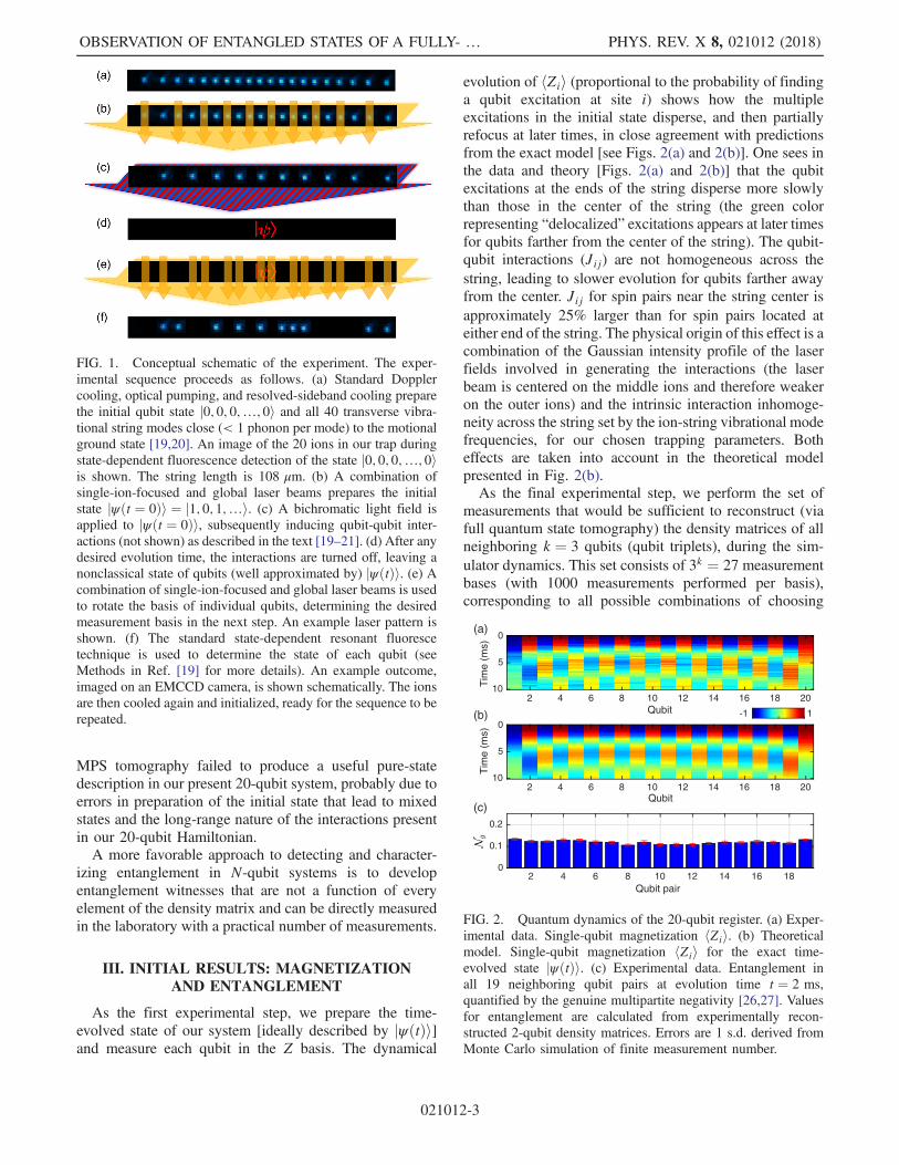
evolution of hZii (proportional to the probability of findinga qubit excitation at site i) shows how the multipleexcitations in the initial state disperse, and then partiallyrefocus at later times, in close agreement with predictionsfrom the exact model [see Figs. 2(a) and 2(b)]. One sees inthe data and theory [Figs. 2(a) and 2(b)] that the qubitexcitations at the ends of the string disperse more slowlythan those in the center of the string (the green colorrepresenting “delocalized” excitations appears at later timesfor qubits farther from the center of the string). The qubit-qubit interactions (Jij) are not homogeneous across thestring, leading to slower evolution for qubits farther awayfrom the center. Jij for spin pairs near the string center isapproximately 25% larger than for spin pairs located ateither end of the string. The physical origin of this effect is acombination of the Gaussian intensity profile of the laserfields involved in generating the interactions (the laserbeam is centered on the middle ions and therefore weakeron the outer ions) and the intrinsic interaction inhomoge-neity across the string set by the ion-string vibrational modefrequencies, for our chosen trapping parameters. Botheffects are taken into account in the theoretical modelpresented in Fig. 2(b).As the final experimental step, we perform the set of

measurements that would be sufficient to reconstruct (viafull quantum state tomography) the density matrices of allneighboring k ¼ 3 qubits (qubit triplets), during the sim-ulator dynamics. This set consists of 3k ¼ 27 measurementbases (with 1000 measurements performed per basis),corresponding to all possible combinations of choosing

Qubit pair2 4 6 8 10 12 14 16 18

0

0.1

0.2

Qubit2 4 6 8 10 12 14 16 18 20

Tim

e (m

s)

0

5

10

Qubit2 4 6 8 10 12 14 16 18 20

Tim

e (m

s)

0

5

10

-1 1

(a)

(b)

(c)

FIG. 2. Quantum dynamics of the 20-qubit register. (a) Exper-imental data. Single-qubit magnetization hZii. (b) Theoreticalmodel. Single-qubit magnetization hZii for the exact time-evolved state jψðtÞi. (c) Experimental data. Entanglement inall 19 neighboring qubit pairs at evolution time t ¼ 2 ms,quantified by the genuine multipartite negativity [26,27]. Valuesfor entanglement are calculated from experimentally recon-structed 2-qubit density matrices. Errors are 1 s.d. derived fromMonte Carlo simulation of finite measurement number.

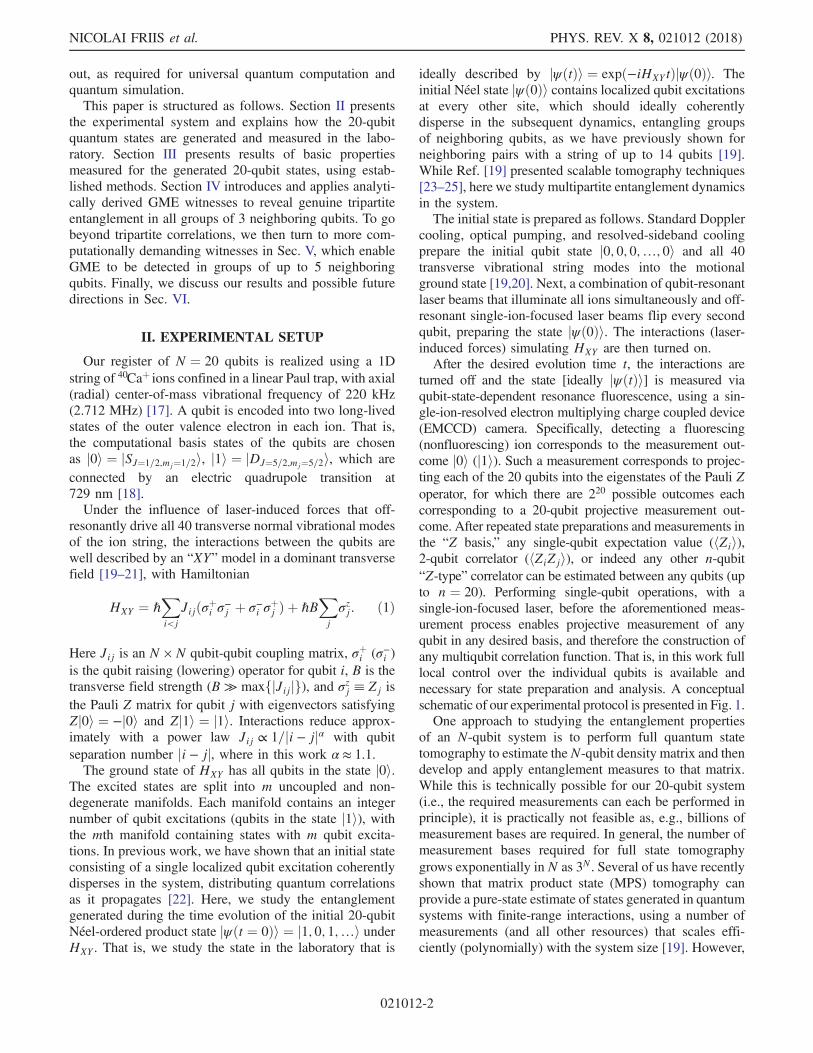
FIG. 1. Conceptual schematic of the experiment. The exper-imental sequence proceeds as follows. (a) Standard Dopplercooling, optical pumping, and resolved-sideband cooling preparethe initial qubit state j0; 0; 0;…; 0i and all 40 transverse vibra-tional string modes close (< 1 phonon per mode) to the motionalground state [19,20]. An image of the 20 ions in our trap duringstate-dependent fluorescence detection of the state j0; 0; 0;…; 0iis shown. The string length is 108 μm. (b) A combination ofsingle-ion-focused and global laser beams prepares the initialstate jψðt ¼ 0Þi ¼ j1; 0; 1;…i. (c) A bichromatic light field isapplied to jψðt ¼ 0Þi, subsequently inducing qubit-qubit inter-actions (not shown) as described in the text [19–21]. (d) After anydesired evolution time, the interactions are turned off, leaving anonclassical state of qubits (well approximated by) jψðtÞi. (e) Acombination of single-ion-focused and global laser beams is usedto rotate the basis of individual qubits, determining the desiredmeasurement basis in the next step. An example laser pattern isshown. (f) The standard state-dependent resonant fluorescetechnique is used to determine the state of each qubit (seeMethods in Ref. [19] for more details). An example outcome,imaged on an EMCCD camera, is shown schematically. The ionsare then cooled again and initialized, ready for the sequence to berepeated.

OBSERVATION OF ENTANGLED STATES OF A FULLY- … PHYS. REV. X 8, 021012 (2018)

021012-3

three Pauli operators. We carry out a simple scheme (choiceof measured Pauli operators) that allows measurements onall 18 neighboring qubit triplets (out of the 20-qubit string)to be performed in parallel, requiring a total of only twenty-seven 20-qubit measurement bases. From this data set, wecould reconstruct the density matrices of all single qubits,neighboring qubit pairs, and neighboring qubit triplets.Generalizing this approach to arbitrary k, all N − kþ 1groups of neighboring k-qubit density matrices in an N-qubit string can be fully characterized by measuring in 3k

bases (independent of the number of qubits N). For fixed k,this measurement approach is clearly efficient (constantoverhead) in the system size N. We nonetheless stop atk ¼ 3, as the number of measurement bases for k ¼ 4 isalready quite demanding and, as we show, k ¼ 3 is alreadysufficient to observe genuine multipartite entanglement ingroups of up to five qubits.We reconstruct the density matrices of all neighboring

qubit pairs from the experimental data, via the standardmaximum likelihood method, which finds the most likelyphysical density matrix to have produced the data. For eachof the reconstructed 2-qubit states we evaluate the genuinemultipartite negativity N g, an established measure forGME [26,27]. A positive value of N g for a given k-qubitstate implies the existence of genuine k-partite entangle-ment in this state, since N g vanishes for all biseparablestates. For two qubits, N g is directly related to thelogarithmic negativity [28]. More details on N g are givenin Sec. V. From the results one sees that all neighboringqubit pairs become entangled during the time evolution ofthe system, as is shown for t ¼ 2 ms in Fig. 2(c). Errorbars, on properties calculated using the tomographicallyreconstructed density matrices, are derived from the finitenumber of measurements (1000 for each global basis) usedto estimate expectation values and calculated using thestandard Monte Carlo method [29].Naturally, one may wonder if entanglement extends

beyond qubit pairs, for instance, in the form of bipartiteentanglement between distant qubits or in terms of genuinemultipartite entanglement between groups of more thantwo (adjacent) qubits. In fact, one may even be tempted toask, is multipartite entanglement not implied if everyneighboring qubit pair is entangled? The answer to thisquestion is simply no. One can indeed have states thatfeature entanglement in every 2-qubit reduction, yet stillfeature only bipartite entanglement [30]. Nonetheless, intheory, it is often possible to detect GME purely frominspection of the reduced density matrices of overlappinggroups of qubits [16]. This is the basis for our first approachto detecting GME, presented in the next section, where wederive GME witnesses purely from neighboring two-bodyobservables.In general, the task of determining if and how an N-qubit

quantum system is entangled is highly nontrivial. For anarbitrary known mixed state (e.g., reconstructed via full

state tomography), the problem is at least NP hard and eventhe best known relaxations are semidefinite programs(SDPs) that are not feasible beyond 5 qubits with ourcomputers [26,31]. However, if the density matrix is closeto a given pure target state jψTi, then targeted witnesses canbe constructed to detect its entanglement without resortingto full tomography [16]. There, the canonical ansatz wouldbe to estimate the fidelity to the ideal target stateTrðρjψTihψT jÞ and check whether it is above the maximumpossible fidelity of a biseparable state. That is, a corre-sponding witness would be W ¼ β1 − jψTihψT j, whereβ ≔ minAjAjjTrAðjψTihψT jÞjj∞; see, e.g., Ref. [16], Sec. 3.6. While this witness could in principle be successful indetecting GME if the experimental state is indeed veryclose to the intended pure state, it suffers from poor noiseresistance [32] and the task of determining the state fidelityfor arbitrary pure states still requires a number of meas-urement settings that scales exponentially in qubit num-ber [33].For example, if the state is “well conditioned” [33], i.e.,

if only few Pauli-expectation values are of a significantsize and all others vanish, one could estimate the fidelityvia randomized measurements [33] with effort that scalesefficiently in qubit number. Although our states are not wellconditioned, in Ref. [19] we implemented this randomizedmeasurement strategy to obtain a fidelity estimate for a14-qubit version of the states presented here, at one timestep. That experiment required preparing 5 × 105 sequen-tial copies of the state and involved over 5 hours of datataking (with periodic recalibration of experimental param-eters). Numerical simulations of the randomized measure-ment technique applied to the 20-qubit states consideredin this work show that more than 3 times the number ofcopies, and therefore impractical measurement time, wouldbe required to yield accurate fidelity estimations. As such,we aim to develop novel, and more time-efficient,approaches to characterizing entanglement in our 20-qubitsystem. As a first step in this direction, we focus on thedynamics of subsystem entanglement percolating throughthe system and are able to make statements about theentanglement using measurements completed in a few tensof minutes in our system.

IV. GME WITNESSES BASED ON2-QUBIT OBSERVABLES

In this section, we construct analytical witnesses forGME based on 2-qubit observables and use them to detectGME in groups of up to three neighboring qubits (k ¼ 3)within the 20-qubit (N ¼ 20) register. Recall that a (multi-partite) pure state jψi is called biseparable if there exists abipartition AjB such that jψi ¼ jϕiAjχiB for some jϕiA andjχiB, and is called genuinely multipartite entangled other-wise. Mixed states are GME if their density operatorscannot be written as convex combinations of biseparablepure states. For more details, see Appendix A 2.

NICOLAI FRIIS et al. PHYS. REV. X 8, 021012 (2018)

021012-4

Following the observation in the previous section ofstrong entanglement between neighboring qubits, the firsttype of GME witnesses we consider is based on averagefidelities of the 2-qubit density matrices with Bell states. Assuch, only expectation values of pairs of Pauli operators, onk-qubit subsets of choice, are required. Linear combina-tions of these expectation values are then evaluated andcompared to their respective thresholds for biseparablek-qubit states. Surpassing a k-qubit biseparability thresholdthen detects genuine k-partite entanglement.We now present a short technical summary of our

method, and refer the reader to Appendix A for moredetails. The main quantity of interest for detecting k-qubitGME in this section is the k-qubit symmetric average Bell

fidelity F ðkÞBell, which we define as

F ðkÞBell ≔

1

4bk

bk þ

Xki;j¼1i<j

ðjhXiXjij þ jhYiYjij þ jhZiZjijÞ!;

ð2Þ

where bk ¼� k2

�¼ 1

2fðk!Þ=½ðk − 2Þ!�g, and the subscripts

i and j denote operators acting nontrivially only on the ithand jth qubits; i.e., Oi ≡ 11 ⊗ … ⊗ 1i−1 ⊗ Oi ⊗ 1iþ1 ⊗… ⊗ 1N . The operator triple Xi ¼ UiXU

†i , Yi ¼ UiYU

†i ,

and Zi ¼ UiZU†i is chosen unitarily equivalent to the usual

triple of Pauli operators X, Y, and Z, although the unitaryUi ∈ SUð2Þ may be chosen differently for each qubit (for

each i). This ensures that F ðkÞBell can be written as a linear

combination (the absolute values can be replaced byappropriate sign changes) of pairs of Pauli operators. Aswe show in detail in Appendix A, any quantum state of kqubits for which

F ðkÞBell >

(112ð3þ ffiffiffiffiffi

15p Þ for k ¼ 3

14ð1þ ffiffiffi

3p Þ − 1

2k ðffiffiffi3

p− 1Þ for k ≥ 4

ð3Þ

is genuinely k-partite entangled for any choice ofU1;…; Uk.For example, for k ¼ 3 and k ¼ 4 one can detect GME for

F ð3ÞBell >

112ð3þ ffiffiffiffiffi

15p Þ ≈ 0.573 and for F ð4Þ

Bell >18ð3þ ffiffiffi

3p Þ≈

0.592, respectively. Meanwhile, the threshold for k ¼ 2

qubits, F ð2ÞBell > 0.5, is a well-known result.

If the underlying N-partite quantum state is known (theUi are known), one could directly measure all of the 3bk2-qubit correlators hOiOji appearing in Eq. (2) for opti-mally chosen fUig. However, when the optimal localmeasurements are unknown, one strategy is to measurethe 6k k-qubit basis settings corresponding to the set

nOðiÞ

XY;OðiÞYX;O

ðiÞXZ;O

ðiÞZX;O

ðiÞYZ; O

ðiÞZY

oi¼1;…;k

; ð4Þ

where OðiÞAB ¼ Ai

Qi≠jBj, and perform the optimization

when evaluating the corresponding results. From the 2k

outcomes of each of these simultaneous measurements of kqubits one can obtain the expectation values of all pairwisecombinations of Pauli operators.For our purposes, we exploit the fact that the results from

the twenty-seven 20-qubit measurement bases alreadytaken in the laboratory are also sufficient to calculate all

the expectation values appearing in the witnesses F ðkÞBell for

k ¼ 2 and k ¼ 3. That is, they contain as a subset, all the

2-qubit observables required to calculate F ð2ÞBell and F ð3Þ

Bell,without knowledge of the states. The results, for increasingsystem interaction times and for the optimization of the Uilimited to the X-Y plane for each qubit, are shown in Fig. 3.

First, the witness for bipartite entanglement (F ð2ÞBell > 0.5)

reaffirms that all qubits are (bipartite) entangled with theirdirect neighbors throughout the interaction time (from time0.5 to 3.5 ms). Second, genuine tripartite entanglementbetween neighboring qubit triples builds up more slowlyand is initially detected at time 1.5 ms. At time 2 ms, mosttriples of neighboring qubits are genuinely tripartiteentangled, before the GME gradually disappears again atlater times.The experimental uncertainties (error bars) in Fig. 3

originate from a finite number of measurements used toestimate expectation values. Specifically, the error barsshow an estimate of 1 standard deviation of the mean.When estimating the standard deviation of the mean, onemust consider possible correlations between 2-qubitexpectation values if they are estimated from outcomesof the same 20-qubit measurement basis. We estimate therelevant variance as described in Ref. [19] (therein seeSupplemental Material Secs. IV.A.4 and IV.A.5, pp. 9–13).The small deviations between the theoretical and mea-

sured dynamics of F ð2ÞBell and F ð3Þ

Bell in Fig. 3 are due toexperimental imperfections, which we discuss in the nextsection.A number of interesting observations, based on analy-

ses beyond those presented in Fig. 3, are now made. First,up to the evolution time presented in Fig. 3, entanglementbetween any 2-qubits spaced farther apart than directneighbors was never detected–in agreement with the idealtheoretical model. For instance, on these timescales, qubit1 does not directly become entangled with qubit 3 alone,but qubits 1, 2, and 3 do become genuinely tripartiteentangled with each other. In fact, the absence of next-nearest-neighbor pairwise entanglement was necessary todetect 3-qubit GME. Specifically, we found that a GMEwitness based only on the entanglement between directneighbors (see Appendix A 2 b) is not able to verifygenuine tripartite entanglement, and it was only possibleto do so once the (separable) correlations between non-neighboring qubits (e.g., qubits 1 and 3) are also takeninto account.

OBSERVATION OF ENTANGLED STATES OF A FULLY- … PHYS. REV. X 8, 021012 (2018)

021012-5

Second, although there are states for which the witness ofEqs. (2) and (3) could be used to detect GME between morethan 3 parties [34], it is not sensitive enough to do so for thestates presented here in our setup (neither for the theoreticalpredictions nor for the experimental data).To address the question of whether genuine multipartite

quantum correlations occur in groups of more than 3 qubits,in our setup, we hence turn to more computationallydemanding procedures, which we present in the next section.The observed and predicted entanglement peak ampli-

tude and dynamics for qubits near the center and those nearthe ends (Fig. 3) are markedly different. We attribute thosedifferences to the interaction inhomogeneity across thequbit string and boundary effects.

V. GME WITNESSES BASED ONNUMERICAL SEARCH

In this section, we present and apply a method thatemploys a numerical search to find k-qubit witnesses forGME. This search is computationally intensive: an opti-mization is performed that takes computational resourcesthat increase exponentially with k. Finding a GMEwitness operator for mixed 5-qubit states is already atthe practical limit of our available computers and algo-rithms. Nonetheless, we find witnesses that succeed indetecting GME in groups of up to 5 qubits in our 20-qubitexperimental system. In the following, we give a brief

overview of the new witnesses and defer to Appendix B fora more detailed discussion of the technical aspects.We make use of the genuine multipartite negativity (N g),

an established measure for GME [26,27]. A positive valueof N g for a given k-qubit state implies the existence ofgenuine k-partite entanglement in this state, since N g

vanishes for all biseparable states. The N g can be calcu-lated given knowledge of the density matrix [26,27].However, we have not performed a tomographically com-plete set of measurements for more than k ¼ 3 qubits (wedo not have the density matrices for the state in the lab, fork > 3). Our approach, to detect GME in any given group i,

of k qubits, is to find a k-qubit witness operator QðkÞi whose

expectation value provides a lower bound on the k-qubitN g, and which can be written as a function of the set ofmeasurements that were carried out in our experiment. Wenow provide more details on this approach.

We perform a search to find a k-qubit operator QðkÞi ,

subject to two important constraints. First, we search for anoperator which both maximizes the following inequality,

−TrðQðkÞi ρki Þ≡ SðkÞ

i ≤ N gðρki Þ; ð5Þfor a specific k-qubit state of interest ρki , and satisfies the

inequality for all possible k-qubit states. We call QðkÞi a

quantitative entanglement witness (QEW) because it pro-vides a lower bound on N g. It is straightforward to

(a)

(b)

FIG. 3. Entanglement witnesses based on symmetric average Bell fidelities. The experimental results (red) and theoretical predictionsbased on ideal time-evolved state jψðtÞi (blue) for the entanglement witnesses F ð2Þ

Bell and Fð3ÞBell are shown in (a) and (b), respectively. The

horizontally arranged panels show the results at different time steps, 0.0 ms, 0.5 ms, 1.0 ms, etc., with intervals of 0.5 ms during the timeevolution of the 20-qubit chain, starting with 0 ms (the initial state). Within each panel, each dot represents a pair (a) or triple (b) ofneighboring qubits. The horizontal dashed lines indicate the detection thresholds for bipartite [(a) F ð2Þ

Bell > 0.5] and genuine tripartite

entanglement [(b) F ð3ÞBell >

112ð3þ ffiffiffiffiffi

15p Þ ≈ 0.573], respectively. The error bars for each qubit pair or triple represent 1 standard deviation

of the mean in each direction. It can be seen in (a) that all qubits immediately become entangled with their direct neighbors and remainentangled throughout, whereas genuine tripartite entanglement is detected in time step 1.0 ms for the first time. At time step 2.0 ms, thewitness F ð3Þ

Bell indicates that all neighboring qubit triples are genuinely tripartite entangled simultaneously (although the witness is lessthan 1 standard deviation above the threshold for two of these triples).

NICOLAI FRIIS et al. PHYS. REV. X 8, 021012 (2018)

021012-6

constrain the search in this way and also to verify that any

given QðkÞi is a QEW. When searching for the optimal

witness, we use a theoretical model for the time-evolvedk-qubit state for ρki . Second, we include the additional

constraint that theQðkÞi can be written as a linear function of

the k-qubit measurement operators (projectors) that were

done, involving qubit group i. Specifically, we restrict QðkÞi

to the form

QðkÞi ¼

Xs;α

cðkÞi;s;αPðkÞs;α; ð6Þ

where the projectors PðkÞs;α correspond to the marginal

distributions of the twenty-seven 20-qubit projective meas-

urement settings carried out in the lab (Sec. III), and cðkÞi;s;α

denote some coefficients. Here, s and α label, respectively,the qubit outcome and the local basis of the measurements;see also Appendix B 2.

The search for the optimal witnesses operator QðkÞi is

carried out using a semidefinite program. The run time ofthe SDP is polynomial in the dimension of the Hilbert space[35,36], but the dimension of our Hilbert space naturally

increases exponentially with the number of qubits k. Thismakes the optimization demanding already for mediumnumbers of qubits: Our available computational resourcesare not sufficient to determine optimal witnesses for statesof more than 5 qubits.

The QðkÞi which satisfies Eqs. (5) and (6), and maximizes

the left-hand side of Eq. (5), determines an optimal witnesstailored to the target state (from a theoretical model) and the

available measurements. Once this optimal QðkÞi is found we

can calculate its expectation value from the outcomes of themeasurement done on the state in the laboratory. A witness

expectation value (SðkÞi ) larger than zero then detects k-qubit

GME (N g > 0), for the ith group of k qubits.The experimental results for k ¼ 3 presented in Fig. 4(a)

show that all neighboring qubit triplets soon develop GMEduring the dynamics, to within many standard deviations,reaching a maximum at t ¼ 2 ms. Furthermore, for thetimes 2, 2.5, and 3 ms, Figs. 4(b) and 4(c) show that GMEis detected in the majority of all neighboring groups of 4and 5 qubits, to within at least 1 standard deviation ofexperimental uncertainty.Figure 4 compares the witness results obtained from the

data with those derived from two theoretical models. The

(a)

(b)

(c)

FIG. 4. Entanglement witnesses derived by a numerical search. The entanglement witnesses Sð3Þi , Sð4Þ

i , and Sð5Þi (see Sec. V) are shown

in (a)–(c), respectively. The horizontally arranged subpanels show the results at different system evolution time steps with intervals of0.5 ms during the time evolution of the 20-qubit chain, starting with 0 ms (the initial state). Within each panel, each dot represents resultsfor a given triplet [(a) k ¼ 3], quadruplet [(b) k ¼ 4], or quintuplet [(c) k ¼ 5] of neighboring qubits. GME is detected if the witness ispositive. The different theory plots are for the pure model (black circles without error bars) and mixed model (blue triangles with errorbars), as described in the text. The red squares with error bars show experimental data. All error bars show 1 standard deviation of themean and originate from a finite number of numerically simulated measurements per measurement basis (1000).

OBSERVATION OF ENTANGLED STATES OF A FULLY- … PHYS. REV. X 8, 021012 (2018)

021012-7

first “pure” model employs the perfect pure 20-qubit time-evolved state [jψðtÞi] and uses exact knowledge of k-qubitdensity matrices to optimize and apply the witnesses.The witness expectation value for the pure model yields

SðkÞi ¼ N gðρki Þ. Although the pure model succeeds in

qualitatively describing the multipartite entanglementdynamics, the witness expectation values from the dataare generally offset to lower values. A more sophisticated“mixed” model is able to explain part of this offset, whichincludes known imperfections in preparing the initialNeel-ordered state. Specifically, out of 1000 attempts togenerate the Neel state, we observe the correct output state829 times. In the remaining 171 cases, 146 correspond tosingle qubit flip errors and the rest to errors with two ormore qubit flips. We attribute these errors to uncontrolledfluctuations in laser intensity and frequency, and modelthem as leading to the preparation of a statistical mixture ofthose different logical initial states, with correspondingweights. The witnesses used for the data were obtained by asearch involving the mixed-model reduced states for thetargets. We attribute the remaining small differencesbetween data and theory, in Fig. 4, to additional mixingprocesses that occur in the laser-induced qubit-qubitinteractions.The mixed theory predictions in Fig. 4 include error bars

due to the use of a finite number of numerically simulatedmeasurements per measurement basis (1000). Error barsindicate 1 standard deviation of the mean, which isestimated as in Sec. IV, and show that the fluctuations inthe data are largely consistent with those expected fromsuch statistical noise. We conclude that, in order to witness4- and 5-partite GME with greater statistical significance infuture work, we could benefit from taking more measure-ments. However, it will be challenging to ensure that theexperimental configuration remains stable over the longertime required to take such additional measurements.The sizes of the error bars on both data and mixed

theory points, in Fig. 4, increase with increasing k. This canbe understood as follows: there are more measurementoutcomes available in the data for the k ¼ 3 witnesscalculations than for larger k. Amongst the twenty-seven20-qubit measurement bases, 3-qubit measurements arerepeated (duplicated) more often in the measurementpattern than 4-qubit or 5-qubit measurements, leading tobetter statistics.

VI. DISCUSSION AND CONCLUSION

We have experimentally generated and detected thepresence of entanglement in a register of 20 qubits. Inparticular, we detected the dynamical evolution of genuinemultipartite entanglement in the system following aquench, and developed new characterization techniquesto do so. While we cannot say that 20-qubit GME wasgenerated, we can say that every qubit simultaneously

became genuine multipartite entangled with a least two ofits neighbors and, in most cases, three and four of itsneighbors.Our experimental apparatus represents the largest joint

system of individually controllable subsystems to datewhere the presence of entanglement has been demon-strated. Each qubit can be individually controlled andqubit-qubit interactions can be turned on and off as desired(and tuned to have various forms). As such, our system hasthe capability to perform universal quantum simulation andquantum computation.Confirming GME beyond groups of 5 qubits, even

for the ideal states, is currently beyond our availableclassical computational resources and algorithms. A pos-sible approach to overcome that problem is to exploitsymmetries in the system and initial state, to reduce the sizeof the search space for witnesses. Another is to tune theexperimental system Hamiltonian into regimes where moresymmetries are apparent or approximated, e.g., infinite ornearest-neighbor-only qubit-qubit interaction ranges.Finally, witnesses based on average Bell-state fidelities

are straightforward to use and measure in the lab. As withall such witnesses, they detect entanglement without theneed to carry out state tomography and can be evaluatedwith only a few measurements. This can be important forthe detection of weakly entangled states, where estimatesbased on state tomography are known to overestimateentanglement [37]. Our witnesses based on brute-forcenumerical searching have the advantage of placing the leastconstraints on the form of the state in the lab and themeasurements that should be taken: this can be important inthe case of unknown local rotations of qubits during thedynamics. As such, our witnesses should find applicationbeyond the present trapped-ion setting.

ACKNOWLEDGMENTS

The work in Innsbruck was supported by the AustrianScience Fund (FWF) under Grant No. P25354-N20, by theEuropean Commission via the integrated project SIQS,and by the Army Research Laboratory under CooperativeAgreement No. W911NF-15-2-0060. The views and con-clusions contained in this document are those of the authorsand should not be interpreted as representing the officialpolicies, either expressed or implied, of the Army ResearchLaboratory or the U.S. Government. B. L. acknowledgesfunding from the Austrian Science Fund (FWF) throughthe START Project No. Y 849-N20. N. F. and M. Huberacknowledge funding from the Austrian Science Fund(FWF) through the START Project No. Y879-N27 andthe joint Czech-Austrian project MultiQUEST (I 3053-N27).The work in Ulm was supported by an Alexander vonHumboldt Professorship, the ERC Synergy grant BioQ, theEU projects QUCHIP, and the U.S. Army Research OfficeGrant No. W91-1NF-14-1-0133, as well as by computa-tional resources by the state of Baden-Württemberg through

NICOLAI FRIIS et al. PHYS. REV. X 8, 021012 (2018)

021012-8

bwHPC and the German Research Foundation (DFG)through Grant No. INST 40/467-1 FUGG.

APPENDIX A: GME WITNESSES BASED ONBIPARTITE CORRELATORS

In this section, we introduce a method for the detectionof genuine multipartite entanglement in N-qubit systems.This method is based on 2-qubit observables and does notrequire full state tomography. In particular, our detectioncriteria can be phrased as biseparability thresholds foraverage Bell fidelities, i.e., expectation values of linearcombinations of pairs of Pauli operators. At the heart of thismethod lies the anticommutativity theorem (ACT) fromRefs. [38,39], which we use to provide bounds on theaverage Bell fidelities. Although our approach is not able todetect all types of GME in multipartite systems, itsadvantage lies in providing linear entanglement witnessesthat can be practically evaluated with only a few measure-ments. More specifically, our approach does not requireobtaining a good estimate of the N-partite correlationtensor [40,41] with 3N components, but instead only needsat most 6N measurements of strings of N local Paulioperators to test for N-partite GME. As we discuss, thelinearity of the witness also makes it amenable to a simpletreatment of the potentially correlated statistical errorsarising from deriving expectation values of bipartiteobservables from simultaneous measurements of N qubits.Following the brief description of these results in Sec. IV

of the main text, we now present more detailed derivationsof the quantities and bounds that we consider. InAppendix A 1, we briefly define and motivate the basicquantities of interest, before we construct our GME wit-nesses in Appendix A 2.

1. Framework

In this section, we explain the basic quantities andnotions of interest, i.e., the anticommutativity theoremof Ref. [39] and the average Bell fidelities to establish abasis for the more detailed discussion of GME that is tofollow in Appendix A 2.

a. Anticommutativity theorem

Let us consider a set fAngn¼1;2;…;k of self-adjoint,normalized, anticommuting operators on a Hilbert spaceH with dimðHÞ ¼ d, i.e.,

TrfAm; Angþ ¼ TrðAmAn þ AnAmÞ ¼ 2dδmn; ðA1Þfor all m; n ¼ 1;…; k. The ACT [38,39] then states thatfor all states ρ ∈ LðHÞ,

Xkn¼1

hAni2ρ ≤ maxn

hA2niρ: ðA2Þ

A simple example for the applicability of this theorem is theset of single-qubit Pauli operators fX; Y; Zg. Since all ofthese operators anticommute and square to the identity, theACT then simply requires that

hXi2ρ þ hYi2ρ þ hZi2ρ ≤ h1iρ ¼ 1: ðA3Þ

In other words, for single-qubit Pauli operators, the ACTis equivalent to demanding that Bloch vectors are (sub)normalized, i.e., positivity of the density operator ρ. A lesstrivial example of the ACT arises for 2 qubits. Consider theset of operators

fX1X2; Y1Y2; Z1Z2; X2X3; Y2Y3; Z2Z3g; ðA4Þ

where the shorthand notation for N-qubit operators is

Oi ≡ 11 ⊗ … ⊗ 1i−1 ⊗ Oi ⊗ 1iþ1 ⊗ … ⊗ 1N; ðA5Þ

and O ∈ fX; Y; Zg. We can sort the six operators in the setdisplayed in Eq. (A4) into three pairs of anticommutingoperators; e.g.,

fX1X2; Y2Y3gþ ¼ 0; ðA6aÞ

fY1Y2; Z2Z3gþ ¼ 0; ðA6bÞ

fZ1Z2; X2X3gþ ¼ 0: ðA6cÞ

Since the spectra of all six operators are f�1g (withtwofold degeneracy), we further have hOiOiþ1i2 ≤ 1,and the ACT theorem hence tells us that)

hX1X2i2ρ þ hY2Y3i2ρ ≤ 1; ðA7aÞ

hY1Y2i2ρ þ hZ2Z3i2ρ ≤ 1; ðA7bÞ

hZ1Z2i2ρ þ hX2X3i2ρ ≤ 1: ðA7cÞ

To see where these bounds can be of use, let us nextexamine fidelities with 2-qubit Bell states.

b. Average Bell-state fidelities

We now want to consider ways of quantifying how closea given 2-qubit state is to a maximally entangled Bell state.To this end, note that the density operators for the fourBell states can be written in a generalized Bloch decom-position as

ρψ− ¼jψ−ihψ−j¼1

4ð11;2−X1X2−Y1Y2−Z1Z2Þ; ðA8aÞ

ρψþ ¼ jψþihψþj¼1

4ð11;2þX1X2þY1Y2−Z1Z2Þ; ðA8bÞ

OBSERVATION OF ENTANGLED STATES OF A FULLY- … PHYS. REV. X 8, 021012 (2018)

021012-9

ρϕ− ¼jϕ−ihϕ−j¼1

4ð11;2−X1X2þY1Y2þZ1Z2Þ; ðA8cÞ

ρϕþ ¼ jϕþihϕþj¼1

4ð11;2þX1X2−Y1Y2þZ1Z2Þ: ðA8dÞ

For any 2-qubit density operator ρ, we can then computethe fidelity with any of the Bell states. For this purpose weuse the Uhlmann fidelity F, given by

F ðρ; σÞ ¼�Tr

ffiffiffiffiffiffiffiffiffiffiffiffiffiffiffiffiffiffiffiσ

pρffiffiffiσ

pq �2

; ðA9Þ

which reduces to

F ðρ; jψihψ jÞ ¼ hψ jρjψi ¼ Trðρjψihψ jÞ ðA10Þ

if one of the arguments is a pure state. For example, for theBell state jψ−i one can use Eq. (A8a) and the fact that allPauli operators are traceless to find

F ðρ;ρψ−Þ¼1

4ð1−hX1X2iρ−hY1Y2iρ−hZ1Z2iρÞ: ðA11Þ

Since the only difference to the fidelities with any of theother Bell states are the relative signs between the differentexpectation values, we can immediately note that thefidelity of ρ with any of the four Bell states is boundedaccording to

F ðρ; ρBellÞ ≤1

4ð1þ jhX1X2ij þ jhY1Y2ij þ jhZ1Z2ijÞ;

ðA12Þ

where we have dropped the subscript for the state ρ on theexpectation values for brevity.

c. Nearest-neighbor average Bell fidelity

When the system consists of more than 2 qubits, we canevaluate the fidelity with 2-qubit Bell states for any two ofthe constituent qubits. For simplicity, let us first considerthe nearest neighbors for now and examine the case of threequbits. The average fidelity with arbitrary nearest-neighborBell states is then

1

2½F ðρ; ρBell;12Þ þ F ðρ; ρBell;23Þ� ≤ FNNBell; ðA13Þ

where we define the quantity FNNBell as the upper bound

FNNBell ≔1

8ð2þ jhX1X2ij þ jhY1Y2ij þ jhZ1Z2ij

þ jhX2X3ij þ jhY2Y3ij þ jhZ2Z3ijÞ; ðA14Þ

but we refer to FNNBell as the average nearest-neighbor Bellfidelity from now on for simplicity. Next, we make use ofthe relation between the 1-norm jjajj1 ¼

Pni¼1 jaij and the

2-norm jjajj2 ¼ ðPni¼1 jaij2Þ1=2 in an n-dimensional vector

space, i.e., the fact that

jjajj1¼Xni¼1

jaij×1¼jða; 1Þj≤ jjajj2�Xn

i¼1

12�

1=2

¼ ffiffiffin

p jjajj2;

ðA15Þ

where we have taken 1 ¼ ð1; 1;…; 1ÞT to be a vector whosecomponents (with respect to whichever basis is chosen for a)are all equal to 1, and we have used the Cauchy-Schwarzinequality jða;bÞj≤ jjajj2jjbjj2. Combining this with theACT theorem from Eq. (A2), we find, e.g.,

jhX1X2ij þ jhY2Y3ij ≤ffiffiffi2

pðhX1X2i2 þ hY2Y3i2Þ ≤

ffiffiffi2

p:

ðA16Þ

Applying the same procedure to the other pairs of expect-ation values of anticommuting operators in Eq. (A14), wearrive at the bound

FNNBell ≤1

8ð2þ 3

ffiffiffi2

pÞ: ðA17Þ

The average nearest-neighbor Bell state fidelity can ofcourse be generalized to N qubits; i.e., the upper bound onthe average nearest-neighbor Bell fidelity is

1

N − 1

XN−1

i¼1

F ðρ; ρBell;iðiþ1ÞÞ ≤ F ðNÞNNBell; ðA18Þ

where we have defined

F ðNÞNNBell ≔

1

4ðN − 1Þ�ðN − 1Þ þ

XN−1

i¼1

XO¼X;Y;Z

jhO1Oiþ1ij�

¼ 1

4ðN − 1Þ ½ðN − 1Þ þ jhX1X2ij þ jhY1Y2ij

þ jhZ1Z2ij þ jhX2X3ij þ jhY2Y3ijþ jhZ2Z3ij þ � � � þ jhXN−1XNijþ jhYN−1YNij þ jhZN−1ZNij�: ðA19Þ

The expression on the right-hand side contains N − 1triples of expectation values. If N is odd, then N − 1 iseven, and each expectation value of an operator OiOiþ1

can be paired with another expectation value of anoperator O0

iþ1O0iþ2 that anticommutes with it; i.e., O;O0 ∈

fX; Y; Zg and fOiOiþ1; O0iþ1O

0iþ2gþ ¼ 0. The bound of

Eq. (A16) can hence be used f½3ðN − 1Þ�=2g times, and wearrive at

NICOLAI FRIIS et al. PHYS. REV. X 8, 021012 (2018)

021012-10

F ðNoddÞNNBell ≤

1

4ðN − 1Þ�ðN − 1Þ þ 3ðN − 1Þ

2

ffiffiffi2

p �

¼ 1

8ð2þ 3

ffiffiffi2

pÞ: ðA20Þ

However, when N is even, one triple of expectation values(without loss of generality for i ¼ N − 1) remains unpairedand can only be bounded by

jhXN−1XNij þ jhYN−1YNij þ jhZN−1ZNij ≤ 3: ðA21Þ

Thus we arrive at the following upper bound on thenearest-neighbor average Bell fidelity for arbitrary N-qubitstates; i.e.,

F ðNÞNNBell ≤

8<:

18ð2þ 3

ffiffiffi2

p Þ ðN oddÞ1

4ðN−1ÞhðN − 1Þ þ 3ðN−2Þ ffiffi2p

2þ 3i

ðN evenÞ:ðA22Þ

d. Symmetric average Bell fidelity

Instead of restricting the analysis to nearest neighbors asin Eq. (A14), one can of course also average over allpairings of 2 qubits, obtaining a quantity that is symmetricwith respect to the exchange of any 2 qubits. Noting thatthere are bN ¼ ðN

2Þ ¼ 1

2fðN!Þ=½ðN − 2Þ!�g different such

pairings, we have the upper bound

1

bN

XNi;j¼1i<j

F ðρ; ρBell;ijÞ ≤ F ðNÞBell; ðA23Þ

with the definition

F ðNÞBell ≔

1

4bN

bN þ

XNi;j¼1i<j

XO¼X;Y;Z

jhOiOjij!: ðA24Þ

For, instance, for 3 qubits we have b3 ¼ 3 and thesymmetric average Bell fidelity reads

F ð3ÞBell ¼

1

12ð3þ jhX1X2ij þ jhX2X3ij þ jhX1X3ij

þ jhY1Y3ij þ jhY1Y2ij þ jhY2Y3ijþ jhZ2Z3ij þ jhZ1Z3ij þ jhZ1Z2ijÞ: ðA25Þ

Here, we have arranged the expectation values such that itbecomes immediately obvious that the triples of operatorscorresponding to expectation values listed directly below orabove each other mutually anticommute. We can then apply

the bound of Eq. (A15) and the ACT of Eq. (A2), e.g., asillustrated for the terms

jhX1X2ij þ jhY1Y3ij þ jhZ2Z3ij≤

ffiffiffi3

pðjhX1X2ij2 þ jhY1Y3ij2 þ jhZ2Z3ij2Þ ≤

ffiffiffi3

p:

ðA26Þ

We thus arrive at the bound

F ð3ÞBell ≤

1

12ð3þ 3

ffiffiffi3

pÞ ¼ 1

4ð1þ

ffiffiffi3

pÞ: ðA27Þ

In fact, the same bound applies for arbitrary numbers ofqubits, since all 3bN expectation values can be collected ingroups of 3 mutually anticommuting operators. To see this,we use an inductive proof. Assume that we have found bNgroups of three anticommuting operators for N ≥ 3 qubitsand we wish to add another qubit. This means that we haveto additionally consider the operators

X1XNþ1; X2XNþ1; X3XNþ1;… ; XNXNþ1;

YNYNþ1; Y1YNþ1; Y2YNþ1;… ; YN−1YNþ1;

ZN−1ZNþ1; ZNZNþ1; Z1ZNþ1;… ; ZN−2ZNþ1:

All columns contain three mutually anticommuting oper-ators for N ≥ 3. If the original 3bN operators can bearranged in mutually anticommuting triples, then alsothe new set of 3bNþ1 operators can be grouped in thisway, which concludes the inductive step. We have alreadydemonstrated that this statement is true for N ¼ 3 and havehence shown that for any N ≥ 3 we have the bound

F ðN≥3ÞBell ≤ F ðNÞmax

Bell ≔1

4ð1þ

ffiffiffi3

pÞ: ðA28Þ

Having established these general bounds that apply forarbitrary quantum states, we next examine how thesebounds can be improved upon when the states in questionare biseparable. This will allow us to formulate criteria forthe detection of genuine multipartite entanglement.

2. GME witnesses

In this section, we establish upper bounds for the nearest-neighbor and symmetric average Bell fidelities for bisepar-able states. These new upper bounds are below therespective bounds of Eqs. (A22) and (A28) and henceleave room for GME states in between. That is, any statesfor which the combinations of expectation values discussedabove provide values beyond these biseparability boundsare GME. As we shall see, the biseparability bounds fornearest-neighbor Bell fidelities are not directly useful fordetecting GME, but these bounds serve as a simple examplefor discussing the method of construction, which will be

OBSERVATION OF ENTANGLED STATES OF A FULLY- … PHYS. REV. X 8, 021012 (2018)

021012-11

helpful for identifying GME witnesses based on symmetricaverage Bell fidelities.

a. Outline of the technique

In the following we consider bipartitions AjB of theset κ ¼ f1; 2;…; Ng of all N qubits; that is, we split κ intotwo sets,

A ¼ fa1; a2;…; akjai ∈ κ; ai ≠ aj ∀ i ≠ jg; ðA29aÞ

B ¼ fb1; b2;…; bN−kjbi ∈ κ; bi ≠ bj ∀ i ≠ jg; ðA29bÞ

such that A ∪ B ¼ κ and A ∩ B ¼ ∅. For N qubits, one has2N−1 − 1 different bipartitions.Before we continue, let us briefly recall the definitions

of biseparability and genuine multipartite entanglement.In general, a pure, N-partite state jψi ∈ H1;2;…;N ¼ H1 ⊗H2 ⊗ …HN is called k-separable if it can be written as atensor product with respect to some partition of H1;2;…;N

into k ≤ N subsystems. As a special case of this definition,a pure state is called biseparable if it can be written asa tensor product with respect to some bipartition, i.e., ifthere exists a bipartition AjB such that jψi ¼ jϕiAjχiB.Conversely, a pure state jψi ∈ H1;2;…;N that is not bisepar-able is called genuinely N-partite entangled. A mixed statewith density operator ρ is considered to be genuinelymultipartite entangled if it cannot be written as a convexcombination of biseparable states, that is, if it cannot bewritten as

ρbisep ¼Xi

pijψ ðiÞbisepihψ ðiÞ

bisepj; ðA30Þ

whereP

ipi ¼ 1 with 0 ≤ pi ≤ 1 and jψ ðiÞbisepi are bisepar-

able pure states. Note that the jψ ðiÞbisepi for different i can be

separable with respect to different bipartitions.Now, consider a bipartition AjB and an operator OiOj

such that i ∈ A and j ∈ B. If the system is in a pure statejψi that is separable with respect to to this bipartition, i.e., ifjψiAB ¼ jϕiAjχiB, then we have

hOiOjiψ ¼ hOiiϕhOjiχ : ðA31Þ

When we have a triple of operators XiXj, YiYj, and ZiZj

for such a separable state across AjB, we have

jhXiXjij þ jhYiYjij þ jhZiZjij¼ jhXiij jhXjij þ jhYiij jhYjij þ jhZiij jhZjij≤Yn¼i;j

ffiffiffiffiffiffiffiffiffiffiffiffiffiffiffiffiffiffiffiffiffiffiffiffiffiffiffiffiffiffiffiffiffiffiffiffiffiffiffiffiffiffiffiffiffiffiffiffiffiffiffiffijhXnij2 þ jhYnij2 þ jhZnij2

q≤ 1; ðA32Þ

where we have used the Cauchy-Schwarz inequality in thesecond-to-last step and the subnormalization of the Blochvector in the last step. The inequality Eq. (A32) can be usedto bound the Bell fidelities for pure biseparable states fordifferent bipartitions.As an example, consider again the nearest-neighbor

average Bell fidelity for three qubits from Eq. (A14).For the bipartition 1j23, we can apply (A32) to the firstthree expectation values in Eq. (A14), while the remainingthree can each be bounded by 1. A similar argument can bemade for the bipartition 12j3 by exchanging the roles of thetwo triples of expectation values, such that

F 1j23;12j3NNBell ≤

1

8ð2þ 1þ 3Þ ¼ 3

4; ðA33Þ

where the superscripts indicate that the inequality issatisfied for states that are biseparable with respect to (atleast one of) the listed bipartitions. When we examine thebipartition 2j13, the situation is slightly different, sinceEq. (A32) can be used for all expectation values, and wehave

F 2j13NNBell ≤

1

8ð2þ 1þ 1Þ ¼ 1

2: ðA34Þ

Any pure 3-qubit state that is separable with respect to oneor more of these bipartitions (any pure, biseparable stateof three qubits) must hence satisfy FNNBell ≤ 3

4. Moreover,

since any mixed state is considered to be biseparable whenit can be written as a convex combination of biseparablepure states (not necessarily with respect to the samebipartition), all mixed, biseparable states must also respectthis bound. Conversely, the first 3 qubits of any state ρfor which

1

8ð2þ jhX1X2ij þ jhY1Y2ij þ jhZ1Z2ij

þ jhX2X3ij þ jhY2Y3ij þ jhZ2Z3ijÞ >3

4ðA35Þ

are genuinely 3-partite entangled.

b. Nearest-neighbor average Bell fidelityas GME witness

In principle, the nearest-neighbor Bell fidelity couldhence provide a detection criterion for GME that can begeneralized to N qubits. However, at this point a remark onthe detection power of this quantity is in order, since evensome paradigmatic cases of genuinely tripartite entangledstates for 3 qubits cannot be detected with this bound. That

is, for the 3-qubit GHZ and W states jψ ð3ÞGHZi and jψ ð3Þ

W i(or the local unitarily equivalent 2-excitation Dicke state

jψ ð3ÞD;2i), given by

NICOLAI FRIIS et al. PHYS. REV. X 8, 021012 (2018)

021012-12

jψ ð3ÞGHZi ¼

1ffiffiffi2

p ðj000i þ j111iÞ; ðA36aÞ

jψ ð3ÞW i ¼ 1ffiffiffi

3p ðj100i þ j010i þ j001iÞ; ðA36bÞ

jψ ð3ÞD;2i ¼

1ffiffiffi3

p ðj110i þ j101i þ j011iÞ; ðA36cÞ

one finds nearest-neighbor average Bell fidelities of

F ð3ÞNNBellðjψ ð3Þ

GHZiÞ ¼1

2; ðA37aÞ

F ð3ÞNNBellðjψ ð3Þ

W iÞ ¼ 2

3; ðA37bÞ

F ð3ÞNNBellðjψ ð3Þ

D;2iÞ ¼2

3; ðA37cÞ

whereas the corresponding bound for detecting GME is 34.

One can hence try to improve the method or find analternative. One way to improve the bound is by way oftaking into account the purity of the biseparable states. Thatis, if we consider again the worst-case bipartition 1j23 for 3qubits under the assumption that the state is separable withrespect to this cut, i.e., that jψi123 ¼ jϕi1jχi23, we have

F 1j23NNBell ≤

1

8ð2þ

ffiffiffiffiffiffiffiffiffiffiffiffiffiffiffiffiffiffiffiffiffiffiffiffiffiffiffiffiffiffiffiffiffiffiffiffiffiffiffiffiffiffiffiffiffiffiffiffiffiffiffiffijhX2ij2 þ jhY2ij2 þ jhZ2ij2

qþ jhX2X3ij þ jhY2Y3ij þ jhZ2Z3ijÞ

¼ 1

8

�2þ jbj þ

X3n¼1

jtnnj�; ðA38Þ

where we have used the Bloch vector b of the second qubitand the correlation tensor t ¼ ðtmnÞ of qubits 2 and 3. Inother words, the state jχi23 can be written in a generalizedBloch decomposition as

ρχ ¼ jχihχj ¼ 1

4

�1þ b · σ⊗ 1þ1⊗ c · σþ

X3i;j¼1

tijσi⊗ σj

�;

ðA39Þ

where σ ¼ ðσnÞ is the vector of Pauli operatorsðσ1 ¼ X; σ2 ¼ Y; σ3 ¼ ZÞ. Now, since jχi23 is a pure state,we have Trðρ2χÞ ¼ 1, which translates to

1

4

�1þ jbj2 þ jcj2 þ

X3m;n¼1

jtmnj2�

¼ 1; ðA40Þ

and we can hence derive the bound

jbj2 þX3n¼1

jtnnj2 ≤ 3: ðA41Þ

Interpreting jbj and jtnnj (n ¼ 1, 2, 3) as coordinates in R4,we find that Eq. (A41) defines a four-dimensional sphere ofradius

ffiffiffi3

p. The sum of the coordinates is then maximal

when all coordinates take the same valueffiffiffiffiffiffiffiffi3=4

p. Inserting

into Eq. (A38), we then get the bound

F 1j23NNBell ≤

1

8

�2þ 4

ffiffiffi3

4

r �¼ 1

4ð1þ

ffiffiffi3

pÞ ≈ 0.683 013:

ðA42Þ

Since the bipartition 12j3 is equivalent and for 2j13 we

have the lower value F 2j13NNBell ≤

12, the “improved” bisepar-

ability bound for the nearest-neighbor average Bell fidelityfor three qubits is 1

4ð1þ ffiffiffi

3p Þ ≈ 0.683 013. This value is

still above the fidelity 23obtained for pure GME states of 3

qubits in Eq. (A44). In addition, we have also conducted anumerical search which did not reveal any pure 3-qubitstates with nearest-neighbor average Bell fidelities beyond23. At the same time, one can find biseparable states that

give values for F ð3ÞNNBell that are very close to

23. For instance,

for the state ρbisep ¼ j0ih0j1 ⊗ ρ23, where j0i1 is aneigenstate of Z, and the (nearly pure) state ρ has Blochvectors b ¼ c ¼ ð0; 0; 0.447ÞT and a diagonal correlation

matrix t ¼ diagf0.894;−0.894; 1g, we find F ð3ÞNNBell ¼

0.654375. We therefore conclude that, in their presentform, GME witnesses based on the nearest-neighboraverage Bell fidelity are practically irrelevant for 3 qubitsand there is no reason to expect an improvement for morethan 3 qubits.We therefore now continue with an analysis of a different

quantity, the symmetric average Bell fidelity.

c. Symmetric average Bell fidelity as GME witness

In this section, we discuss the usefulness of the sym-metric average Bell fidelity as a witness for GME. To thisend, we again need to identify the bipartitions providing the

worst (largest) upper bound for F ðNÞBell under the assumption

of separability with respect to the respective bipartition.Since the combination of expectation values that weconsider now is symmetric under the exchange of any 2qubits, this task is rather straightforward.First, we consider the case of 3 qubits separately, where

all three possible bipartitions (i.e., 1j23, 2j13, and 12j3)are equivalent. If the system state is pure and separable withrespect to any of these bipartitions, two of the triplesof expectation values in Eq. (A25) are “cut” by thebipartition and can be bounded by 1, while the remainingtriple consists of three commuting observables, whose

OBSERVATION OF ENTANGLED STATES OF A FULLY- … PHYS. REV. X 8, 021012 (2018)

021012-13

expectation values are jointly bounded by 3. For anylabeling of the 3 qubits, we hence have

F 1j23Bell ≤

1

12ð3þ 1þ 1þ 3Þ ¼ 2

3: ðA43Þ

As we discussed in Appendix A 2 b, this bound has to becompared with values achievable with pure GME states.For the 3-qubit GHZ-, W-, and 2-excitation Dicke states,we find symmetric average Bell fidelities

F ð3ÞBellðjψ ð3Þ

GHZiÞ ¼1

2; ðA44aÞ

F ð3ÞBellðjψ ð3Þ

W iÞ ¼ 2

3; ðA44bÞ

F ð3ÞBellðjψ ð3Þ

D;2iÞ ¼2

3; ðA44cÞ

which happen to coincide with the corresponding nearest-neighbor average Bell fidelities of Eq. (A44). We musthence try to improve the bound using a similar trick asbefore in Appendix A 2 b. Again assuming a biseparablepure state for the bipartition 1j23, we can write

F 1j23Bell ≤

1

12

�3þ jbj þ jcj þ

X3n¼1

jtnnj�; ðA45Þ

and in analogy to Eq. (A41) we can bound each of themoduli jbj, jcj, and jtnnj (for n ¼ 1, 2, 3) by

ffiffiffiffiffiffiffiffi3=5

p, which

gives the bound

F ð3ÞbisepBell ≤

1

12

3þ 5

ffiffiffi3

5

r !¼ 1

12ð3þ

ffiffiffiffiffi15

pÞ ≈ 0.572749:

ðA46Þ

Using numerical optimization, we can also provide apure biseparable state that comes very close to this bound.That is, for the state ρbisep ¼ j0ih0j1 ⊗ ρ23, where j0i1 is aneigenstate of Z, and the pure state ρ has Bloch vectorsb ¼ c ¼ ½0; 0; ð1= ffiffiffi

2p Þ�T and a diagonal correlation matrix

t¼diagfð1= ffiffiffi2

p Þ;−ð1= ffiffiffi2

p Þ;1g, we find F ð3ÞBell ¼ 0.569 036.

As before, the pure state biseparability bound extends tomixed states via convexity. Thus, any 3-qubit state forwhich the combination of (moduli of) expectation values onthe right-hand side of Eq. (A25) exceeds 1

12ð3þ ffiffiffiffiffi

15p Þmust

be genuinely tripartite entangled.Second, let us turn to the case of 4 qubits, where we are

interested in bounding the quantity

F ð4ÞBell ¼

1

24ð6þ jhX1X2ij þ jhX1X3ij þ jhX1X4ij

þ jhX2X3ij þ jhX2X4ij þ jhX3X4ijþ jhY1Y2ij þ jhY1Y3ij þ jhY1Y4ijþ jhY2Y3ij þ jhY2Y4ij þ jhY3Y4ijþ jhZ1Z2ij þ jhZ1Z3ij þ jhZ1Z4ijþ jhZ2Z3ij þ jhZ2Z4ij þ jhZ3Z4ijÞ: ðA47Þ

For any pure state that is separable with respect to abipartition into 1 versus 3 qubits, we find three triplesof expectation values that are cut (each bounded by 1),while three triples pertaining to the same subsystem can becombined into mutually anticommuting triples, eachbounded by

ffiffiffi3

p, obtaining

F 1j234Bell ≤

1

24ð6þ 3þ 3

ffiffiffi3

pÞ ¼ 1

8ð3þ

ffiffiffi3

pÞ ≈ 0.591506:

ðA48Þ

Instead, we can also use the bound arising from the purityof the reduced state of qubits 234 of the biseparable purestate. Since the local dimension for these three qubits is23 ¼ 8 and we have 12 terms appearing [the Bloch vectorsof the ith qubit jaij (i ¼ 2, 3, 4) and the correlations tensorelements jt23nnj, jt24nnj, and jt34nnj for n ¼ 1, 2, 3], we find thebound

F 1j234Bell ≤

1

24

�6þ 12

ffiffiffiffiffiffiffiffiffiffiffi8 − 1

12

r �¼ 1

8ð6þ

ffiffiffiffiffi84

pÞ ≈ 0.631881:

ðA49Þ

However, this upper bound is larger than that arising justfrom using the ACT, and Eq. (A49) is therefore of nofurther consequence.The only other possible type of bipartition of 4 qubits

is into two sets of 2 qubits. In this case, four triples are cutby the bipartition, but in each set one triple of unpairedoperators remains (jointly bounded by 3), such that we have

F 12j34Bell ≤

1

24ð6þ 4þ 3þ 3Þ ¼ 2

3: ðA50Þ

As we have argued before, a biseparability bound for 3qubits that is larger or equal to 2

3is not very useful since

even pure GME states (e.g., the 4-qubit Dicke state withtwo excitations) achieve only this value. We hence againturn to using the purity of the subsystems for a biseparablestate jψi1243 ¼ jϕi12jχi34. In this case, the symmetricaverage Bell fidelity can be bounded by

NICOLAI FRIIS et al. PHYS. REV. X 8, 021012 (2018)

021012-14

F 12j34Bell ≤

1

24

�6þja1j ja3jþ ja1j ja4jþ ja2j ja3jþ ja2j ja4j

þX

n¼1;2;3

jt12nnjþX

n¼1;2;3

jt34nnj�: ðA51Þ

Here, we encounter a different optimization problem thanbefore, since we no longer seek to maximize the sum ofabsolute values, but some quantities (e.g., ja1j and ja3j) arecoupled. However, due to the symmetric form (with respectto the exchange of qubits 12 with 34) of the expression, wemay write

F 12j34Bell ≤

1

24

�6þ2

�ja1j2þja2j2þ

Xn¼1;2;3

jt12nnj��

: ðA52Þ

We hence seek to maximize fða; tÞ ¼ 3tþ 2a2 under theconstraints 2a2 þ 3t2 ¼ 3 and a2 ≤ 1, which is achievedfor a ¼ 1 and t ¼ ð1= ffiffiffi

3p Þ, and hence

F 12j34Bell ≤

1

24

�6þ2

�2þ 3ffiffiffi

3p��

¼ 1

12

�5þ

ffiffiffi3

p �≈0.561004:

ðA53Þ

Since this value is smaller than that for the bipartition 1j234in Eq. (A48), we can identify the bound of Eq. (A48) withthe biseparability bound for the symmetric average Bellfidelity for 4 qubits; i.e.,

F ð4ÞbisepBell ≤

1

8

�3þ

ffiffiffi3

p �≈ 0.591 506: ðA54Þ

For more than 4 qubits, we can derive more generalexpressions using the method based on the ACT, whilethe exponentially increasing subsystem dimension makesbounds based on the subsystem purity unfeasible. Considera system of N ≥ 4 qubits that is in a separable pure statewith respect to a bipartition into a single qubit versus theremaining N − 1 qubits. One may then identify N − 1triples of expectation values that factorize and can bebounded by one, while the remaining bN−1¼bN−ðN−1Þtriples form anticommuting sets of three which are eachbounded by

ffiffiffi3

p. We thus have

F 1j23…NBell ≤

1

4

�1þ 1

bN

nN − 1þ ½bN − ðN − 1Þ�

ffiffiffi3

p o�

¼ 1

4

�1þ

ffiffiffi3

p �−

1

2N

� ffiffiffi3

p− 1�; ðA55Þ

where we have made use of the fact that ½ðN−1Þ=bN �¼f½ðN−1Þ2ðN−2Þ!�=ðN!Þg¼ð2=NÞ. Note that, as required,this bound reduces to the result obtained in Eq. (A48) forN ¼ 4. Intuitively, it is now clear that other bipartitions willprovide smaller upper bounds, since more operators are

affected by the factorization. The exception being the caseN ¼ 4, where we have already seen that the separation intotwo sets of two provides a larger upper bound since eachside then features unpaired expectation values.To confirm this, let us briefly consider bipartitions into 2

and N − 2 qubits for N ≥ 5. In such a case, 2ðN − 2Þexpectation values factorize for the respective pure, sepa-rable states, and one triple of operators pertaining to the twoisolated qubits cannot be paired with anticommutingpartners, whereas bN−2¼bN−ðN−2Þ¼bN−2ðN−1Þþ1triples of operators can be matched up in this way. Thus,we have

F 12j34…NBell ≤

1

4

�1þ 1

bN

h2ðN−2Þþ3þðbN−2Nþ3Þ

ffiffiffi3

p i�

¼1

4

�1þ

ffiffiffi3

p ��1þ 1

bN

�−1

N

� ffiffiffi3

p−1�: ðA56Þ

This expression provides a smaller upper bound when

1

2N

� ffiffiffi3

p− 1�>

1

4bN

�1þ

ffiffiffi3

p �ðA57aÞ

⇒ 1 >1

2ðN − 1Þ�1þ

ffiffiffi3

p �2; ðA57bÞ

which is the case for N ≥ 5, as expected. We have alsoconfirmed that this intuition holds for bipartitions into kversus N − k qubits for 3 ≤ k ≤ N − 3. We can henceformulate the biseparability bound based on the symmetricaverage Bell fidelity for arbitrary numbers of qubits in thefollowing way. For any biseparable state of N qubits, thesymmetric average Bell fidelity satisfies

F ðNÞBell ≤ F ðNÞbisep

Bell

≔

8<:

112

�3þ ffiffiffiffiffi

15p �

for N ¼ 3

14

�1þ ffiffiffi

3p �

− 12N

� ffiffiffi3

p− 1�

for N ≥ 4:

ðA58Þ

Conversely, any state that violates the inequality Eq. (A58)is genuinely N-partite entangled. Before we discuss thepractical usefulness of these witnesses, let us brieflyanalyze possible improvements in Appendix A 2 d.

d. Optimizing GME witnesses basedon bipartite fidelities

To keep the notation simple during the derivations, wehave thus far used only expectation values of pairs of thesame Pauli operators, i.e., of the form jhOiOjij. In practice,this corresponds to measuring the real part of certain off-diagonal elements of the density operator. To see this,consider a 2-qubit state ρ and note that

OBSERVATION OF ENTANGLED STATES OF A FULLY- … PHYS. REV. X 8, 021012 (2018)

021012-15

Tr½ρðX1X2 þ Y1Y2Þ� ¼ 4Reðh01jρj10iÞ: ðA59Þ

Of course, the off-diagonal element h01jρj10i need not bereal for a given 2-qubit state. Here, one may note that thederivations of all bounds that we have considered so far areinvariant under local unitary transformations. That is, wecan replace the triple of operators fXi; Yi; Zig for the ithqubit with the rotated operators Oi ¼ UiOiU

†i for any

unitary Ui. This is the case because such a rotation maps atriple of anticommuting operators to another triple ofanticommuting operators, and the length of the Blochvectors also is left invariant. For instance, one couldperform a rotation in the equatorial plane of the Blochsphere, and map

Xi ↦ Xi ¼ cosðθiÞXi − sinðθiÞYi; ðA60Þ

Yi ↦ Xi ¼ sinðθiÞXi þ cosðθiÞYi: ðA61Þ

In the example of Eq. (A59) this means we can pick θ1 ¼ 0and θ2 ¼ −ðπ=2Þ to obtain

Tr½ρðX1X2 þ Y1Y2Þ� ¼ Tr½ρðX1Y2 − Y1X2Þ�¼ 4Imðh01jρj10iÞ: ðA62Þ

In particular, there exist rotation angles θ1 and θ2 suchthat

Tr½ρðX1X2 þ Y1Y2Þ� ¼ 4jh01jρj10ij: ðA63Þ

In general, one hence has the freedom of N independenttransformations Ui ∈ Uð2Þ to optimize the GME witnessespresented so far. In an experimental setting, this optimi-zation can be done a priori if the quantum state ρ that oneexpects to produce (approximately) in the experiment isknown. However, if the underlying state is unknown,one may also measure all combinations of 2-qubit Paulioperators for all pairs of qubits within the set of N qubits[amounting to 9bN ¼ 9

2NðN − 1Þ 2-qubit measurements]

and perform the optimization on the experimental data. For

instance, the results for F ð3ÞBell presented in Fig. 3 of the main

text have been obtained by such a postprocessing ofavailable measurement data, and the corresponding opti-mization has been restricted to rotations in the X-Y planes,as shown in Eq. (A61).In addition to a posteriori optimization, one may

perform some of these 2-qubit measurements on differentpairs simultaneously if the individual outcomes for eachqubit are recorded. For instance, in a register of N ≥ 3qubits one may obtain the expectation values of X1X2 andX2Y3 from measuring the first and second qubit in theeigenbasis of X and the third in the eigenbasis of Y andrecording all three outcomes in each run. For measurementsof this kind, such as have been performed in our

experiment, data used to estimate different 2-qubit expect-ation values may be correlated, which has to be taken intoaccount in the calculation of the estimate for the variance ofthe GME witness. This is explained in more detail inRef. [19] (therein see Supplemental Material Secs. IV. A. 4and IV. A. 5, pp. 9–13).

e. Usefulness of GME witnesses basedon bipartite fidelities

A crucial question when employing these witnesses is ofcourse whether or not states exist that can be detected bythem. To analyze this problem, we compare the upper

bound F ðNÞbisepBell for biseparable states with the upper bound

F ðNÞmaxBell for arbitrary states from Eq. (A28) by calculating

their distance as a function of the number of qubits. We findthe expression

F ðNÞmaxBell − F ðNÞbisep

Bell ¼8<:

112

ffiffiffi3

p ð3 − ffiffiffi5

p Þ ðN ¼ 3Þ12N ð

ffiffiffi3

p− 1Þ ðN ≥ 4Þ;

ðA64Þ

where the numerical values for 3 and 4 qubits are 112

ffiffiffi3

p ð3 −ffiffiffi5

p Þ ≈ 0.110 264 and 18ð ffiffiffi

3p

− 1Þ ≈ 0.091 506 4, respec-tively. The gap between the bounds is hence largestfor N ¼ 3, and shrinks with increasing number ofqubits. It is hence expected that there is some finiteN for which no GME states exist that are detected byour witnesses, and at this point, we cannot say forwhich N this occurs.For 3 qubits, we have already found examples of

genuinely tripartite entangled states that can be detected,

i.e., the 3-qubit W state jψ ð3ÞW i and the 2-excitation Dicke

state jψ ð3ÞD;2i, which provide symmetric average Bell fidel-

ities of 23. The experimental results discussed in the main

text (see Fig. 3) further show that F ð3ÞBell is also a useful

witness for mixed states produced in realistic situations.

Beyond 3 qubits, the witnesses F ðN≥4ÞBell (optimized only

over rotations in the X-Y plane; see Appendix A 2 d) havenot been able to detect GME in our experimental setting.However, we know that 4-qubit states exist, e.g., the 4-qubit

2-excitation Dicke state jψ ð4ÞD;2i which could be detected in

this way, since F ð4ÞBellðjψ ð4Þ

D;2iÞ ¼ 23. Unfortunately, the 2-

excitation Dicke state for 5 qubits only provides a value of

F ð5ÞBellðjψ ð5Þ

D;2iÞ ¼ 0.6, whereas F ðNÞbisepBell ¼ 1

20ð7þ 3

ffiffiffi3

p Þ≈0.61. Tentative searches for other 5-qubit states for which

F ð5ÞBell exceeds the biseparability bound have been unsuc-

cessful thus far. The question of whether GME states existthat can be detected with our method for N ≥ 5 henceremains open.

NICOLAI FRIIS et al. PHYS. REV. X 8, 021012 (2018)

021012-16

APPENDIX B: CONSTRUCTION OF WITNESSESBASED ON NUMERICAL SEARCH

1. Genuine multipartite negativity

We now discuss the genuine negativity (GMN) ofRef. [27] that we use to quantify GME in the experiment.We present its definition as a convex-roof construction andthe alternative way of writing it in terms of a semidefiniteprogram, which turns it into a numerically computablemeasure of entanglement for an arbitrary mixed state.We start by introducing the notation and presenting

preliminary definitions. Note that a bipartition of f1;…;Ngcan be specified by a subset A ⊂ f1;…; Ng and itscomplement A ¼ f1;…; NgnA. With this, we define thepartial transposition on A for an operator XA ⊗ XA, whereXA and XA act on the Hilbert spaces associated to A and A,respectively, as ðXA ⊗ XAÞTA ¼ XT

A ⊗ XA. The definitionthen extends to any operator on the N-particle Hilbert spaceby linearity. Next, the negativity of a bipartite quantumstate ρ with respect to the bipartition AjA is given bythe sum of the negative eigenvalues of the partially trans-posed density matrix; i.e., N AjAðρÞ ¼

Pλi≤0jλiðρTAÞj ¼

N AjAðρÞ ¼ ½ðkρTAk1 − 1Þ=2�, where λiðXÞ denotes the itheigenvalue of an operator X. With this, the GMN of anN-particle state ρ is given by

N gðρÞ ¼ minfpi;ρig

Xi

piminAjA

N AjAðρiÞ; ðB1Þ

where the inner minimization is over the possible biparti-tions AjA of f1;…; Ng and the outer minimization is overdecompositions ρ ¼Pipiρi, where fpigi is a probabilitydistribution and ρi are density matrices. For pure states, thisreduces to N gðjψihψ jÞ ¼ minAjAN AjAðjψihψ jÞ.For mixed states the GMN can still efficiently be

computed using numerical tools from the field of semi-definite programming. This follows from the fact that theGMN is given by the optimal value of the followingoptimization:

N gðρÞ ¼ maxQ;PA;RA

½−TrðQρÞ�

Q ¼ KA þQTAA ∀ AjA;

0 ≤ KA and 0 ≤ RA ≤ 1; ðB2Þ

where Q, KA, and RA are operators acting on the Hilbertspace. The GMN is zero for all (bi)separable states and,therefore, a nonzero value provides a way to certify GME.More precisely, the GMN is nonzero for any state thatcannot be written as a positive partial transpose (PPT)mixture. Recall that a multipartite state ρ is called a PPTmixture if it admits a mixed state decompositionρ ¼PApAρA, where fpAgA is a probability distributionand ρA has a positive partial transposition (we say, ρA isPPT) with respect to the bipartition AjA. That is, formally,

ρTAA ≥ 0. As noted earlier, a state is called biseparable if itcan be written as a convex combination of states that areseparable with respect to one bipartition AjA. Since anyseparable state is PPT, every biseparable state can bewritten as a PPT mixture. Consequently, a state withnonzero GMN is GME.Moreover, the GMN quantifies the entanglement in the

sense that a state ρ is more entangled than σ ifN gðρÞ ≥ N gðσÞ. The underlying mathematical propertyis that the GMN is nonincreasing under so-called full localoperations and classical communication operations. Inparticular, from this property it follows that no GME statecan be generated from a non-GME state with localoperations only.A further beneficial property of writing the GMN as in

Eq. (B2) is that this yields an entanglement witness, that is,an observable that provides ideally a sharp lower bound tothe GMN as in Eq. (5) in the main text and may be accessedexperimentally. For our purposes note that whether awitness can be measured depends on the measurementsthat are available in our experiment. We therefore discussthose measurements next. The procedure of obtaining theentanglement witnesses that are accessible for us is thendescribed subsequently in Appendix B 3 in more detail.

2. Accessible measurements on k neighboring sites

Here, we discuss the operators that can be measuredlocally on k consecutive sites with the data available in ourexperiment. Our starting point is hence the set of allpossible observables whose measurement outcomes canbe obtained from the 27 measurement settings that wementioned in Sec. III. As we noted there, these measure-ment settings can be used to obtain estimates of theexpectation values of all possible products of the identityand the three Pauli operators on all groups of threeneighboring qubits in the chain of 20 qubits. On suchtriples of neighboring qubits this thus allows us to estimatethe expectation value of any operator, in particular, anypossible entanglement witness. However, the situation isdifferent for more than three neighboring sites. Regardingthis case, recall that in the 27 settings we consider, the 20qubits are measured simultaneously such that the accessibleinformation turns out to be more than just knowing thethree-body reductions of neighboring qubits. Also as aconsequence of how we choose these 27 settings, each ofthem has the property that the local bases in which sites iand iþ 3 are measured are identical. To illustrate what thisimplies for the accessible operators, let us consider theexample of four sites. In terms of projective qubit mea-surements, a basis of operators that we can measure with

the 27 settings is given by B4 ¼ fPð4Þs;αgs;α, where Pð4Þ

s;α

denotes the projector onto the state

js; αi ¼ js1; s2; s3; s4iα1;α2;α3;α1 ; ðB3Þ

OBSERVATION OF ENTANGLED STATES OF A FULLY- … PHYS. REV. X 8, 021012 (2018)

021012-17

where s≡ ðs1; s2; s3; s4Þ ∈ f↑;↓g×4 and α≡ ðα1;α2;α3Þ∈f1;2;3g×3. In words, these operators comprise all projec-tive qubit measurements where the first and the fourth qubitare measured in the same direction. Notably, with the Paulioperators X, Y, and Z, this set of operators spans the samesubspace as the operators fσα1 ⊗ σα2 ⊗ σα3 ⊗ σα1gα, whereα∈ f0;1;2;3g×3 and σ0¼ 1, σ1 ¼X, σ2¼Y, σ3 ¼Z. Forthe construction of the witness we will, however, use theprojectors as our basis set. Accordingly, generalizing this toarbitrary number of sites, we denote the projectors thatform a basis of the operators that can be measured on kconsecutive sites with the 27 settings by Bk. As a furtherremark, let us mention that the number of elements in Bk

grows exponentially with k as jBkj ¼ 27 × 2k.

3. Accessible quantitative entanglement witnesses

Next, we turn to the construction of an entanglementwitness that is fully accessible from the available informa-tion provided by the 27 measurement settings. The mainstep is to solve the optimization given in Eq. (B6) below,which provides a quantitative witness. The witness can thenbe evaluated using the experimental data.We distinguish between a simple entanglement witness,

which is an operatorQ that has a positive expectation valueTrðQρsepÞ ≥ 0 for any separable state ρsep and for whichthere exists at least one entangled state ρ with TrðQρÞ ≤ 0,and a quantitative entanglement witness, i.e., an operatorthat fulfills the property of being an entanglement witnessand additionally provides a lower bound to the GMN via(minus) its expectation value S ¼ −TrðQρÞ of the form

S ≤ N gðρÞ ðB4Þ

for any ρ, as noted in the main text.Now, considering k neighboring sites in the chain of 20

qubits, the available information from the 27 settings isdetermined by the projectors in the set Bk as describedabove. Then, an entanglement witness W is accessible fromthis information if it can be written as a linear combinationof operators from Bk, i.e., if

QðkÞi ¼

Xs;α

cðkÞi;s;αPðkÞs;α; ðB5Þ

with coefficients cðkÞi;s;α ∈ R, since, in this case, it is fullydetermined by the set Bk.

Here, for a given state ρðkÞi (as defined in the main text),

we can optimize over the coefficients cðkÞi;s;α in order to find aquantitative witness that provides the best lower boundto the GMN of ρ. As the computation of the GMN itself,see Eq. (B2), this optimization can be expressed as asemidefinite program. That is, with the definition

pðkÞi;s;α ¼ TrðPðkÞ

s;αρðkÞi Þ, the solution of

SðkÞi ðfPðkÞ

s;α; pðkÞi;s;αgÞ ¼ max

ci;s;α;KA;RA

�−Xs;α

cðkÞi;s;αpðkÞs;α

�Xs;α

cðkÞi;s;αPðkÞs;α ≥ KA þ RTA

A ∀ AjA;

0 ≤ KA and 0 ≤ RA ≤ 1; ðB6Þ

is the best lower bound of the from SðkÞi ðfPðkÞ

s;α; pðkÞi;s;αgÞ ¼

−TrðQðkÞi ρðkÞi Þ ≤ N gðρðkÞi Þ, with QðkÞ

i a quantitative witnessas in Eq. (B5) and with the coefficients for which themaximum in Eq. (B6) is achieved. Note that for brevity wedenote both the optimization parameters in Eq. (B6) as well

as, in the following, the optimal coefficients by cðkÞi;s;α. As a

further remark, we note that SðkÞi ðfPðkÞ

s;α; pðkÞi;s;αgÞ and the

optimal witness Q depend only on the (accessible) prob-abilities ps;α (and the corresponding projectors), such thatthese quantities are sufficient to determine the bound.In order to obtain the bounds in Fig. 4 we determine an

entanglement witness W that can be decomposed as a sumof projectors as in Eq. (B5) and, hence, it can readily beevaluated using the frequencies measured in the experi-ment. The basic steps to determine a quantitative witnessare then (as also described in the main text) as follows. Wefirst perform a numerical simulation to obtain the time-evolved state ρsimðtÞ and determine its reduced densitymatrices on neighboring sites. Then, for every reductionρXsimðtÞ ¼ TrnX ½ρsimðtÞ�, where X ⊂ f1;…; Ng denotes thesites corresponding to the Hilbert space on which ρXsimðtÞacts on, we solve the optimization of Eq. (B6) (plus some

practical amendments; see Appendix B 4) with pðkÞi;s;α ¼

Tr½PðkÞs;αρ

XsimðtÞ� as input to obtain the witness.

In the numerical simulation we include mixing due to animperfect initial state, as described in the main text. To thisend, we use an initial state that is diagonal in the Z bases asρsimð0Þ ¼

Psfsjsihsj, where jsi≡ js; ð3;…; 3Þi is a state

of the product basis in the Z direction [see Eq. (B3) for thenotation we use] and fs is the frequency of the qubitconfiguration s that we observe using the experimental dataobtained at t ¼ 0 ms. Since, besides the ideal initial statewith alternating qubits, only 42 other configurations withnonzero frequency fs occur, the participating configura-tions are readily evolved separately and mixed in order toobtain a density matrix ρsimðtÞ at later times.The optimization of Eq. (B6) used to determine the QEW

QðkÞi depends on the probabilities pðkÞ

i;s;α but not on the

underlying quantum state ρðkÞi . One may be tempted toinsert experimentally measured estimates for the probabil-

ities pðkÞi;s;α to determine a witness which is optimal for the

(unknown) quantum state of the experiment. However,

there is, in general, no quantum state ρðkÞi which satisfies

NICOLAI FRIIS et al. PHYS. REV. X 8, 021012 (2018)

021012-18

TrðPðkÞs;αρ

ðkÞi Þ ¼ pðkÞ

i;s;α where the pðkÞi;s;α are experimentally

estimated probabilities because the pðkÞi;s;α are affected by

statistical noise from a finite number of measurements. As aconsequence, the optimization may fail to be feasible.

Therefore, we use the probabilities pðkÞi;s;α from the reduced

density matrices of the numerically simulated state ρsimðtÞin the optimization of Eq. (B6) in order to determine the

QEW QðkÞi . After QðkÞ

i has been determined, its expectationvalue, which provides the lower bounds in Fig. 4, isdetermined from the experimental data.Instead of using the numerically simulated state ρsimðtÞ

to determine the witness, we furthermore test statesobtained from quantum state tomography. For this purposewe split the data into two statistically independent sets ofsamples and use one set for tomography and the other toevaluate the witness. We pursue this strategy using globalpure-state MPS reconstruction and find no significantadvantage of the approach over using the numericallysimulated state ρsimðtÞ as a starting point.After performing the optimization of Eq. (B6) to

determine QðkÞi , we perform an additional optimization

which makes the QEW more robust to statistical noise andexperimental imperfection. The lower bounds presented inFig. 4 of the main text are based on this improved witness,and the remaining steps are discussed in the next section.

4. Additional conditions for practical witnesses

To make the witnesses less sensitive to experimental

imperfections, we modify the coefficients cðkÞi;s;α as discussedin the following. The major step is to reduce the number ofnonzero coefficients. This can be achieved by employing aninteractive l1-relaxation method with weight updating thatis intended to find sparse solutions [42]. We incorporatethis into our considerations by solving the followingoptimization in the nth iteration step:

mincðkÞ;ni;s;α

Xi;s;α

jcðkÞ;ni;s;α jjcðkÞ;n−1i;s;α j þ ϵ

Tr½ðQðkÞ;ni −QðkÞ;0

i ÞρðkÞi � ≤ ϵ;

QðkÞ;ni ≥ KA þ RTA

A ∀ AjA; ðB7Þ

where QðkÞ;ni ¼Ps;αc

ðkÞ;ni;s;α P

ðkÞs;α, and initially the coefficients

are obtained from Eq. (B6) with cðkÞ;0s;α ¼ cðkÞi;s;α with thecoefficients that are found from solving Eq. (B6). We allowthe bound to diminish by at most ϵ from the optimal one inorder to find a sparse solution. In the results we present, wechoose ϵ ¼ 5 × 10−3 and use three iteration steps. Exceptfor the tolerance ϵ, this step does not deteriorate the bound.We then further add two simple constraints to Eqs. (B6) and

(B7). First, we choose the coefficients as cðkÞ;ni;s;α ∈ ½−1; 1�.Second, we add the semidefinite condition KA ≤ 1 toEq. (B6). Note that this condition has previously beenemployed in an earlier version of the GMN; seeRefs. [26,27]. However, there the quantitative witnessesare exact functions of the operators KA and RA, whereashere they are only related via an inequality. SolvingEqs. (B6) and (B7) with the constraints introduced in this

section results in the bounds SðkÞi presented in the main text.

We observe that the additional modifications significantlyhelp to improve the lower bounds.

[1] M. B. Plenio and S. Virmani, An Introduction to Entangle-ment Measures, Quantum Inf. Comput. 7, 1 (2007).

[2] R. Horodecki, P. Horodecki, M. Horodecki, and K.Horodecki, Quantum Entanglement, Rev. Mod. Phys. 81,865 (2009).

[3] N. Brunner, D. Cavalcanti, S. Pironio, V. Scarani, and S.Wehner, Bell Nonlocality, Rev. Mod. Phys. 86, 419 (2014).

[4] M. A. Nielsen and I. L. Chuang, Quantum Computation andQuantum Information (Cambridge University Press,Cambridge, U.K., 2000).

[5] S. Lloyd, Universal Quantum Simulators, Science 273,1073 (1996).

[6] N. Gisin, G. Ribordy, W. Tittel, and H. Zbinden, QuantumCryptography, Rev. Mod. Phys. 74, 145 (2002).

[7] H. J. Kimble, The Quantum Internet, Nature (London) 453,1023 (2008).

[8] D. J. Wineland, J. J. Bollinger, W.M. Itano, F. L. Moore,and D. J. Heinzen, Spin Squeezing and Reduced QuantumNoise in Spectroscopy, Phys. Rev. A 46, R6797 (1992).

[9] S. F. Huelga, C. Macchiavello, T. Pellizzari, A. K. Ekert,M. B. Plenio, and J. I. Cirac, On the Improvement ofFrequency Standards with Quantum Entanglement, Phys.Rev. Lett. 79, 3865 (1997).

[10] V. Giovannetti, S. Lloyd, and L. Maccone, QuantumMetrology, Phys. Rev. Lett. 96, 010401 (2006).

[11] N. Friis, D. Orsucci, M. Skotiniotis, P. Sekatski, V. Dunjko,H. J. Briegel, and W. Dür, Flexible Resources for QuantumMetrology, New J. Phys. 19, 063044 (2017).

[12] G. Vidal, Efficient Classical Simulation of SlightlyEntangled Quantum Computations, Phys. Rev. Lett. 91,147902 (2003).

[13] T. Monz, P. Schindler, J. T. Barreiro, M. Chwalla, D. Nigg,W. A. Coish, M. Harlander, W. Hänsel, M. Hennrich, and R.Blatt, 14-Qubit Entanglement: Creation and Coherence,Phys. Rev. Lett. 106, 130506 (2011).

[14] C. Song, K. Xu, W. Liu, C. P. Yang, S.-B. Zheng, H. Deng,Q. Xie, K. Huang, Q. Guo, L. Zhang, P. Zhang, D. Xu, D.Zheng, X. Zhu, H. Wang, Y. A. Chen, C. Y. Lu, S. Han, andJ. W. Pan, 10-Qubit Entanglement and Parallel LogicOperations with a Superconducting Circuit, Phys. Rev.Lett. 119, 180511 (2017).

[15] X.-L. Wang, L.-K. Chen, W. Li, H.-L. Huang, C. Liu, C.Chen, Y.-H. Luo, Z.-E. Su, D. Wu, Z.-D. Li, H. Lu, Y. Hu,X. Jiang, C.-Z. Peng, L. Li, N.-L. Liu, Y.-A. Chen, C.-Y. Lu,

OBSERVATION OF ENTANGLED STATES OF A FULLY- … PHYS. REV. X 8, 021012 (2018)

021012-19

and J.-W. Pan, Experimental Ten-Photon Entanglement,Phys. Rev. Lett. 117, 210502 (2016).

[16] O. Gühne and G. Tóth, Entanglement Detection, Phys. Rep.474, 1 (2009).

[17] C. Hempel, Ph.D. thesis, University of Innsbruck, 2014.[18] P. Schindler, D. Nigg, T. Monz, J. T. Barreiro, E. Martinez,

S. X. Wang, S. Quint, M. F. Brandl, V. Nebendahl, C. F.Roos, M. Chwalla, M. Hennrich, and R. Blatt, A QuantumInformation Processor with Trapped Ions, New J. Phys. 15,123012 (2013).

[19] B. P. Lanyon, C. Maier, M. Holzäpfel, T. Baumgratz, C.Hempel, P. Jurcevic, I. Dhand, A. S. Buyskikh, A. J. Daley,M. Cramer, M. B. Plenio, R. Blatt, and C. F. Roos, EfficientTomography of a Quantum Many-Body System, Nat. Phys.13, 1158 (2017).

[20] Petar Jurcevic, Ph.D. thesis, University of Innsbruck, 2017.[21] K. Kim, M.-S. Chang, R. Islam, S. Korenblit, L.-M. Duan,

and C. Monroe, Entanglement and Tunable Spin-SpinCouplings between Trapped Ions Using Multiple Trans-verse Modes, Phys. Rev. Lett. 103, 120502 (2009).

[22] P. Jurcevic, B. P. Lanyon, P. Hauke, C. Hempel, P. Zoller,R. Blatt, and C. F. Roos, Quasiparticle Engineering andEntanglement Propagation in a Quantum Many-BodySystem, Nature (London) 511, 202 (2014).

[23] M. Cramer and M. B. Plenio, Reconstructing QuantumStates Efficiently, arXiv:1002.3780.

[24] S. T. Flammia, D. Gross, S. D. Bartlett, and R. Somma,Heralded Polynomial-Time Quantum State Tomography,arXiv:1002.3839.

[25] M. Cramer, M. B. Plenio, S. T. Flammia, R. Somma, D.Gross, S. D. Bartlett, O. Landon-Cardinal, D. Poulin, andY.-K. Liu, Efficient Quantum State Tomography, Nat.Commun. 1, 149 (2010).

[26] B. Jungnitsch, T. Moroder, and O. Gühne, Taming Multi-particle Entanglement, Phys. Rev. Lett. 106, 190502 (2011).

[27] M. Hofmann, T. Moroder, and O. Gühne, AnalyticalCharacterization of the Genuine Multiparticle Negativity,J. Phys. A 47, 155301 (2014).

[28] M. B. Plenio, Logarithmic Negativity: A Full EntanglementMonotone That Is Not Convex, Phys. Rev. Lett. 95, 090503(2005).

[29] B. Efron and R. Tibshirani, Bootstrap Methods for StandardErrors, Confidence Intervals, and Other Measures ofStatistical Accuracy, Stat. Sci. 1, 54 (1986).

[30] Take, for example, the k-qubit state with density operator

ρ¼ 12ð⊗k=2

i¼1jϕþ

2i−1;2iihϕþ2i−1;2ijþ ⊗

k=2

i¼1jϕþ

2i;2iþ1ihϕþ2i;2iþ1jÞ, where

k is assumed to be even and jϕþi;ji ¼

ð1= ffiffiffi2

p Þðj0iij0ij þ j1iij1ijÞ, with the second index being

understood as modulo k. The state ρ is a convex combina-tion of (k=2)-separable states, yet the reduced state ρi;iþ1 ¼12ðjϕþihϕþj þ 1

41Þ of every pair of neighboring qubits is

entangled.[31] C. Lancien, O. Gühne, R. Sengupta, and M. Huber,

Relaxations of Separability in Multipartite Systems: Semi-definite Programs, Witnesses and Volumes, J. Phys. A 48,505302 (2015).

[32] For qubits β ≤ 12and thus the best possible noise resistance is

50% white noise. While this may seem strong from abipartite intuition, many multipartite states in fact haveasymptotically perfect white noise resistance, i.e., approach-ing 100% polynomially in system dimension, which wouldinevitably be missed by such simple witness constructions.

[33] S. T. Flammia and Y.-K. Liu, Direct Fidelity Estimationfrom Few Pauli Measurements, Phys. Rev. Lett. 106,230501 (2011).

[34] For instance, pure 4-qubit Dicke states with two excitations

would yield F ð4ÞBell ¼ 2

3> 0.592. Beyond 4 qubits, we cannot

say with certainty whether states exist for which our witnesscould certify GME in principle. For a discussion, seeAppendix A 2 c.

[35] S. Boyd and L. Vandenberghe, Convex Optimization,7th ed. (Cambridge University Press, Cambridge, U.K.,2004).

[36] R. H. Tütüncü, K. C. Toh, and M. J. Todd, Solving Semi-definite-Quadratic-Linear Programs Using SDPT3, Math.Program., Ser. B 95, 189 (2003).

[37] C. Schwemmer, L. Knips, D. Richart, H. Weinfurter, T.Moroder, M. Kleinmann, and O. Gühne, Systematic Errorsin Current Quantum State Tomography Tools, Phys. Rev.Lett. 114, 080403 (2015).

[38] G. Tóth and O. Gühne, Entanglement Detectionin the Stabilizer Formalism, Phys. Rev. A 72, 022340(2005).

[39] A. Asadian, P. Erker, M. Huber, and C. Klöckl, Heisenberg-Weyl Observables: Bloch Vectors in Phase Space, Phys.Rev. A 94, 010301(R) (2016).

[40] J.-Y. Wu, H. Kampermann, D. Bruß, C. Klöckl, and M.Huber, Determining Lower Bounds on a Measure ofMultipartite Entanglement from Few Local Observables,Phys. Rev. A 86, 022319 (2012).

[41] C. Klöckl and M. Huber, Characterizing MultipartiteEntanglement without Shared Reference Frames, Phys.Rev. A 91, 042339 (2015).

[42] E. J. Candes, M. B. Wakin, and S. P. Boyd, EnhancingSparsity by Reweighted l1 Minimization, J. Fourier Anal.Appl. 14, 877 (2008).

NICOLAI FRIIS et al. PHYS. REV. X 8, 021012 (2018)

021012-20