Embed Size (px)
Citation preview

128 KART OG PLAN 2–2013
Observasjon validering, modellering – historiske linjer og nye resultater i norsk forskning om jordens tyngdefelt1
Christian Gerlach, Michal Šprlák, Katrin Bentel and Bjørn R. Pettersen
Vitenskapelig bedømt (refereed) artikkel
Christian Gerlach et. al: Observation, validation, modeling – historical lines and recent results in Norwegian gravity fieldresearch
KART OG PLAN, Vol. 73, pp. 128–150, POB 5003, NO-1432 Ås, ISSN 0047-3278
The history of modern gravity field research stretches back to the second half of the 19th century, when international co-operation was established through the foundation of the Mitteleuropäische Gradmessung, the predecessor of today’s In-ternational Association of Geodesy (IAG). Norway was among the first nations collaborating in this international en-deavor and is thus one of the oldest member states of IAG. Gravity field activities in Norway were in many cases inspiredby and connected to the activities and resolutions of IAG, e.g., the establishment of the European gravimeter calibrationbaseline in the 1950s. This also holds for some of the recent gravity field related projects on which we report in this paper.They are carried out at the Norwegian University of Environmental and Life Sciences in Ås (UMB), formerly the Agri-cultural University of Norway (NLH). Olav Mathisen, to whom we dedicate this contribution on the occasion of his 80th
birthday in 2012, was engaged in gravity field research over the past decades, first as an observer and geodesist at theGeographical Survey of Norway (now called Kartverket) and later as professor of surveying at NLH. We use this occasionto put the current research activities into a historical perspective. We present new validation results of the gravity gradi-ometry satellite mission GOCE by comparison with deflections of the vertical in Norway (many of which Olav Mathisenhad observed) and discuss mathematical techniques for regional gravity field representation with radial basis functionsas an alternative to classical approaches.
Keywords: gravimetry, deflections of the vertical, GOCE, gravity field modeling, radial basis functions
Christian Gerlach, prof. II, dr. Commission for Geodesy and Glaciology, Bavarian Academy of Sciences and Humanities,Alfons-Goppel-Str. 11, 80539 München. E-mail: [email protected]
Michal Šprlák,2 Katrin Bentel and Bjørn R. Pettersen. Department of mathematical sciences and technology, Drøbakve-ien 31, NO-1432 Ås.
Historical remarksThe theoretical foundations for gravimetricmeasurements and gravity field modelingwere developed in the 17th and 18th centuryand are connected to the works of, amongothers, Galilei, Huygens, Newton, Bouguer,Clairaut, Laplace, Legendre and Poisson.Gravimetric studies at that time were usedto determine the value of the gravitationalconstant, the mean density and mass of theEarth as well as its flattening. Until 1830,gravimetric observation methods were based
on the oscillation periods of pendulums. Gra-vimetric surveys were carried out withtransportable field equipment (see, e.g., Tor-ge, 1989). Both absolute and relative pen-dulums were constructed, the latter only pro-viding gravity differences with respect to anabsolute reference point. The first determi-nations of gravity in Norway were made byEdward Sabine at two stations in Hammer-fest and Trondheim in 1823 (Hansteen,1825). Around that time, Sabine also recog-nized the possibility to estimate the mass
1. Denne artikkelen er skrevet til Festskrift Olav Mathisen. Alle artiklene fikk ikke plass i festskriftet (nr. 1, 2013) og denne artikkelen måtte vente. Vi trykker den her som en fortsettelse av festskriftet.
2. New address from 2013: Department of Mathematics, Faculty of Applied Science, University of West Bohemia, Univerzitní 22, 306 14 Plze , Czech Republic

Observasjon validering, modellering – historiske linjer og nye resultater
KART OG PLAN 2–2013 129
distribution of the upper layer of the Earthby means of gravity measurements (Sabine,1825; see also Torge, 1989). The accuracy ofgravity observations at that time was in therange of 5–10 mGal or worse.
It was, however, not before the 1860s,when intense scientific research on the gravi-ty field began. Before that time, geodetic sur-veys had been carried out by several countri-es as basis for topographic maps or in order tostudy the general shape of the Earth, i.e. theflattening of the ellipsoid. In Norway, astro-nomical measurements had been carried outsince 1780 for the purpose of positioning andorientation of trigonometric networks (Pet-tersen 2009). Later, measurements were car-ried out by Christopher Hansteen in 1816/17and 1847 to determine the longitude differen-ce between Oslo, Stockholm and Copenhagen(see Jelstrup, 1929; Pettersen 2002, 2006). Asignificant intensification of scientific rese-arch on the gravity field of the Earth startedin the 1860ies. Johann Jakob Baeyer, officerof the Prussian General Staff and director ofthe Geodetic Institute in Berlin, proposed tothe Prussian King in 1861 to establish an of-ficial cooperation between central Europeanstates to study the shape of the Earth. Heproposed to investigate various effects whichnever before had been taken care of in geode-tic meridian arc measurements or topograp-hic surveys, namely the precise determinati-on of the curvature of the figure of the Earthand its scientific implications, e.g., its depen-dency on topography. In Baeyer’s terminologythe figure of the Earth is the mathematical fi-gure as defined by Gauss (1828), i.e. an equi-potential surface at mean sea level, later cal-led the geoid by Listing (1873). The king ac-cepted Baeyer’s proposal for a Mitteleuropäis-che Gradmessung and ordered the PrussianMinistry of Foreign Affairs to invite the cen-tral European states to participate. By 1862,15 states had expressed their willingness tocooperate. Norway was one of them. Dedica-ted national commissions were founded tocarry out the work. In 1864 the representati-ves of the participating countries met in Ber-lin for the first international geodetic confe-rence. They agreed to perform trigonometricand astronomical observations as well as pre-cision leveling. Referring thereby each of the
national leveling networks to mean sea levelforms the basis for comparing heightsthroughout Europe. Determination of thecurvature of the Earth was based on astrono-mical observations, from which deflections ofthe vertical are derived as the difference bet-ween the astronomical and the ellipsoidal co-ordinates. In Norway, astronomical observa-tions were carried out between 1865 and1894 by astronomy professors Carl FredrikFearnley and Hans Geelmuyden. A geodeticmeridian arc was connected to the Swedisharc in the south and was extended to Levan-ger north of Trondheim. Accurate baselineswere established at each end (Pettersen2007). Astronomical activities were then in-terrupted until the 1920ies when H. Heniecarried out astronomical observations inSpitzbergen and H.J. Jelstrup began expan-ding the net of Laplace stations in mainlandNorway.
The aims of the Mitteleuropäische Grad-messung, although formulated in 1864, arestill on the agenda today. Of course the met-hodologies have changed. National triangu-lation networks have been replaced by globalnavigation satellite systems (GNSS). Deflec-tions of the vertical are only observed in spe-cial applications because in most cases thehuge amount of terrestrial gravity data ma-kes them obsolete for modeling the finestructures of the geoid. The scientific objecti-ves, however, are still valid today. One of theobjectives of ESA’s satellite mission GOCE(ESA, 1999) is to support global unificationof height systems, a task very similar to the1864 idea of comparing the national heightsystems throughout Europe. At the time ofBaeyer, deflections of the vertical were requi-red to reduce trigonometrically observedzenith distances for determination of precisetrigonometric heights. Geoid heights wererequired for reduction of measured arclengths down to the surface of the ellipsoid.Today, geoid heights – besides their use ingeophysical applications – are used for trans-formation between ellipsoidal heights as de-rived from GNSS and heights of the nationalleveling networks, e.g. orthometric heights.Recently, Canada and U.S.A. have decided tocompletely abolish leveling networks for therealization of their vertical reference frames.

Bedømt (refereed) artikkel Gerlach, Šprlák, Bentel and Pettersen
130 KART OG PLAN 2–2013
Instead, a precise geoid model will define thevertical datum. It can be foreseen that thisapproach will be followed by many more co-untries in the future.
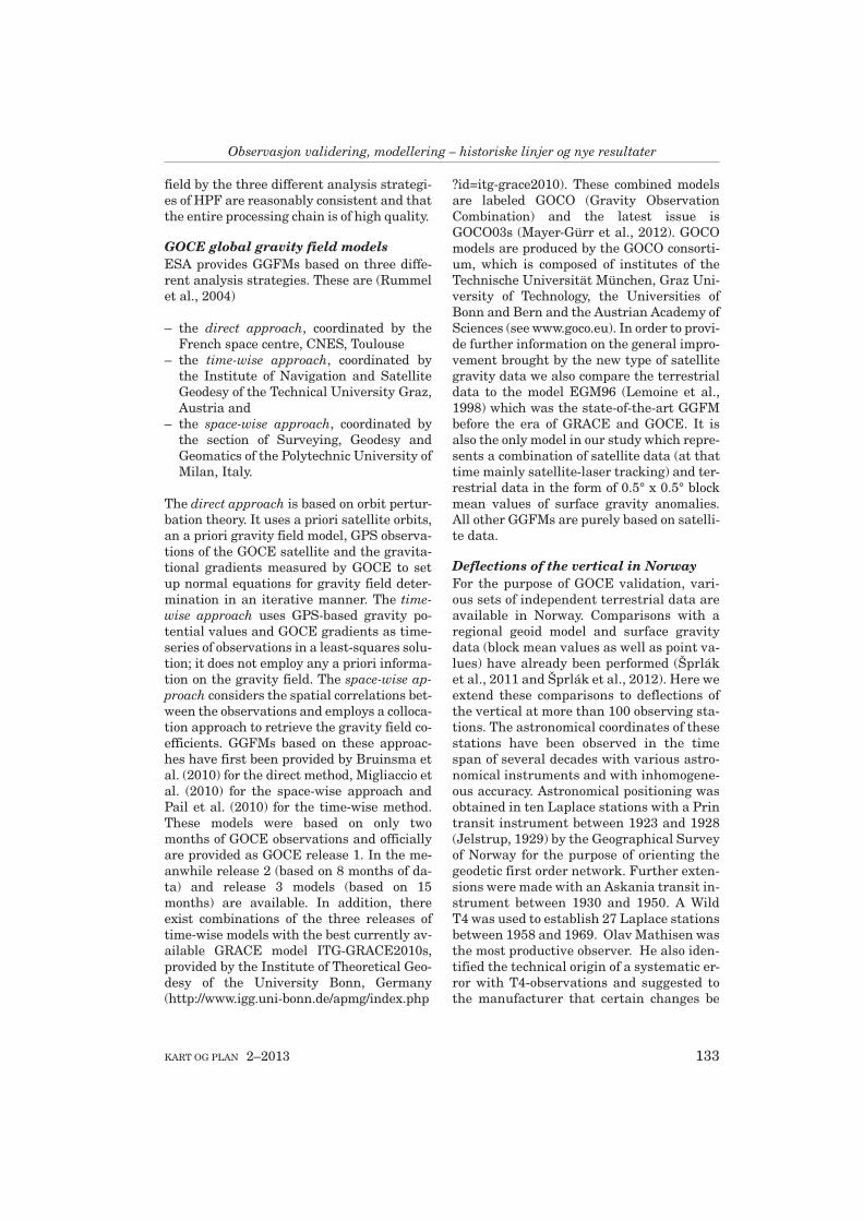
Getting back to the time after the 1864Berlin conference, the Mitteleuropäische Grad-messung gave rise to an advent in gravimetricresearch. In 1887 Robert Daublebsky vonSterneck, staff of the Austro-Hungarian mili-tary, developed a relative pendulum appara-tus for field measurements with an accuracyof 5 mGal and observation times of about1 day per station. It was used in many coun-tries and by 1912 already 2500 gravity valueswere observed. In 1892 a set of Sterneck pen-dulums were purchased by the Norwegiancommission. One of these instruments ac-companied Fridtjof Nansen on his Fram ex-pedition to the polar seas (1893–96). The shipfroze in for three years and drifted with theocean currents. It served as an observatory ofseveral phenomena and obtained the firstgravity observations at sea. The other instru-ment was used at 6 stations in northern Nor-way in 1893 and at 8 stations in southernNorway in 1894 by physics professor O.E.Schiøtz (1894, 1895). He used the UniversityObservatory in Oslo as his reference site andlisted his results with 5 decimals. The resultsfit well to those obtained by Nansen at the re-ference point in Oslo prior to his expedition.In his 1895 report Schiøtz also computed gra-vity anomalies and correlated them to geolo-gical features. The instrument used by Schi-øtz was still in use when G. Jelstrup of theGeographical Survey of Norway (NGO) con-nected a new reference point in the Geologi-cal Museum in Oslo to the reference point inPotsdam, Germany. With the advent of relati-ve gravimeters it became more and more im-portant to realize a precise absolute gravitybase to which the relative values could be lin-ked. The old Potsdam System of 1909 wasestablished to provide a global referencepoint based on the measurements carried outby Kühnen and Furtwängler between 1898and 1904 (Kühnen and Furtwängler, 1906).
International geodetic research collabora-tions were ended by World War I and only afew neutral states tried to keep the organiza-
tion alive – Norway among them. In 1919geodetic research collaboration was reorga-nized as a section of the newly establishedInternational Union of Geodesy and Geophy-sics (IUGG). Later this section became theInternational Association of Geodesy (IAG)with its thematic commissions3. At the 1922IUGG General Assembly in Rome the needfor many more gravity measurements wasexpressed to allow geoid determination bas-ed on the equation developed by George Ga-briel Stokes in 1849 (see equation (5)). At thesame time, isostatic theories were establis-hed and Vening-Meinesz developed his sea-gravimeter for applications in submarines.In addition, the first static relative gravime-ters were developed. They allowed higherprecision and a much shorter observationtime per station. Instruments by LaCosteand Romberg were built since 1939 and tho-se by Worden by 1948. In 1946 G. Nörgaardof the Danish Geodetic Institute measuredthe gravity difference between Oslo and Co-penhagen with two Nörgaard gravimeters(Trovaag and Jelstrup, 1950; see Figure 1).In 1948 NGO purchased Nörgaard gravime-ter number 382 for a thorough survey of Nor-way. From 1948–1949 several gravity con-nections were measured between Oslo andother capitals. In the sequel gravity was me-asured along the lines of the first order leve-ling network. Later NGO acquired additio-nal relative gravimeters by Worden in 1953and by LaCoste and Romberg in 1969. At the1951 IUGG assembly recommendationswere given for the establishment of gravime-ter calibration lines. Following these recom-mendations, the Department of Geodesy andGeophysics at the University of Cambridgemade its pendulum apparatus available, andNorway established a calibration line fromHammerfest via Tromsø, Bodø, Trondheimand Oslo to Bad Harzburg, Germany. At the1954 IUGG assembly it was decided to estab-lish a European calibration base by exten-ding the Norwegian line via Munich to Rome.
By 1956 the Norwegian section of the linecontained 102 points. About 3600 gravity me-asurements had been conducted along leve-ling lines. By 1962 the gravity net contained
3. In IAG’s current structure Commission 2 deals with the gravity field. For a list of sections and commissions established since 1948 see Drewes, 2012.

Observasjon validering, modellering – historiske linjer og nye resultater
KART OG PLAN 2–2013 131
5200 stations, many with multiple observa-tions. The reference station was at the Geolo-gical Museum in Oslo, which was tied to seve-ral other reference stations in Denmark,England, Finland, Germany, Iceland, Swe-den, and USA (Sømod, 1957). One of the mostremarkable ties is probably the one to Ancho-rage, Alaska, which was performed on SAS’sinaugural flight on the North Pole air-route.However, until the end of the 1960ies therehad been no attempts to compute a Norwegi-an geoid model from the available gravity da-ta. Later it was Olav Mathisen who had usedexisting deflections of the vertical to determi-ne a first regional geoid model over Norway.Today regional geoid models are based ongravity values rather than deflections of thevertical, because much more gravity observa-tions are available (in Norway more than70.000 gravity stations compared to approxi-mately 120 astronomical stations). However,deflection data is very useful for validationpurposes as will be shown below.
When LaCoste & Romberg gravimeterswere introduced in Norway, the gravimetricnet was reobserved and extended during the1970s. This forms the core of the nationalgravity database. Olav Mathisen was thelast observer in Norway to use the Nörgaardgravimeter, and the first one to use a LaCos-te & Romberg (Bjørn Geirr Harsson 2012,private communication). Absolute gravime-try was re-introduced to Norway in the 1990s
when free fall instruments visited fromabroad. Since 2004, the Norwegian Univer-sity of Environmental and Life Sciences atÅs has conducted its own observing programwith its state-of-the-art free-fall absolutegravimeter FG5 number 226. This has led toa new database of very accurate absolute sta-tions (Breili et al., 2010). Time series of ab-solute gravimetry at selected stations allowderivation of current epoch reference values.Recomputation of the national gravity net tocurrent epoch is used to validate results fromthe GOCE satellite (Šprlák et al., 2012).
Observation, validation and modeling of the Earth’s gravity fieldGravity field modeling can be performed onglobal or regional scales. The two approachesdiffer in application, resolution, input dataand mathematical modeling. Global mode-ling deals with the deviations of the true gra-vity field from the gravity field of a meanEarth ellipsoid at resolutions of typically 10to 50 km. Regional modeling cares for the de-viations of the fine structures of the geoidfrom such a global model. Therefore, globaland regional modeling cannot be seen as in-dependent of each other, but global modelsprovide the background for regional refine-ments. Basis for all global gravity field mo-dels is the observation of the mean globalfield from satellites. In the beginning of thesatellite era, satellite positions were obser-ved by cameras and satellite laser rangingfrom the ground. Deviations between the ob-served orbit and a nominal orbit computedfrom a priori knowledge were used to impro-ve global gravity field models. Today, thereare dedicated satellite gravity missions ofwhich the U.S.-German Gravity and ClimateExperiment GRACE (Tapley et al., 2004) andESA’s Gravity and Steady-State Ocean Cir-culation Explorer GOCE (ESA, 1999) are themost important. The two missions are com-plimentary. GRACE observes the globalstructures of the gravity field with very highprecision. This allows detection of tiny tem-poral variations, caused, e.g., by seasonal va-riations in ground water or by melting of thelarge ice sheets in Greenland and Antarctica.However, the spatial resolution is limited to
Figure 1: Nörgaard-Gravimeter from Elek-trisk Malmletning A/B, Stockholm [source:Trovaag and Jelstrup, 1950].

Bedømt (refereed) artikkel Gerlach, Šprlák, Bentel and Pettersen
132 KART OG PLAN 2–2013
a few hundred kilometers for monthly gravi-ty field models and about 200 km for theirlongterm average. GOCE is designed to ob-serve finer structures of the gravity fielddown to spatial resolutions of about 80–100km. Modelers try to combine such satellitedata with terrestrial data in an optimal waywith respect to the error budget of the avai-lable data. Therefore it is worthwhile to in-vestigate the optimal mathematical parame-terization of the regional field as well as totest the quality of the data by mutual compa-risons and to investigate possible systematicdeviations. Thus, application of the new typeof satellite observations requires selection ofa proper mathematical formulation as wellas data validation. At the 2011 IUGG assem-bly, IAG established a joint study group(JSG0.3) to investigate different methodolo-gies in regional gravity field modeling as wellas a joint working group (JWG2.3) for the as-sessment of GOCE geopotential models. Theauthors of the current paper are engaged inboth of these groups and basic ideas as well
as current results of their work are reportedin the subsequent sections.
GOCE validation with astronomical observations in NorwayGeneral concept of validationThe objective of GOCE to determine the glo-bal gravity field to the level of 1–2 cm interms of geoid heights and 1 mGal in termsof gravity for spatial scales of 100 km or less,is extremely demanding. In order to ensurethe quality of the GOCE products, ESA hasset up a complex data processing strategyconsisting of data preprocessing, internaland external calibration of the observationsand the estimation of global gravity field mo-dels (GGFM). These models are providedas sets of spherical harmonic coefficients
of degree and order (d/o) l and m,which allow computation of the gravitationalpotential (or any other gravity field functio-nal) according to
(1)
The maximum degree L is connected to thespatial resolution Δ (half wavelength) by thefollowing rule of thumb
(2)
The GGFMs are produced by the High-levelProcessing Facility (HPF) comprising a consor-tium of 10 European university and researchinstitutions (Rummel et al., 2004). They followthree competitive strategies for data filteringand analysis (Pail et al., 2011). We may thusexpect differences between the different solu-tions. In view of the demanding quality requi-rements and the different processing strategi-es, validation of the GGFMs is a crucial task. Itis performed by comparison with independentdata (Koop et al., 2001) which allows verificati-on of the entire data processing chain (observa-tion, calibration, analysis).
In the present paper we present validationresults of the GOCE GGFMs provided by
ESA through HPF by comparison with de-flections of the vertical in Norway. Basically,this corresponds to a validation of the incli-nation of GOCE geoid models in north-southand east-west directions. Similar compari-sons have been performed by Voigt et al.(2010) and Voigt and Denker (2011) using de-flections of the vertical in Germany and byHirt et al. (2011) using deflection data in Eu-rope and Australia. Of course also other ty-pes of terrestrial data have been employedfor validation, e.g. gravity values (see e.g.Šprlák et al., 2012), regional or global geoidmodels (see e.g., Šprlák et al., 2011; Janákand Pito ák, 2011) and point values of geoidheights derived from GPS/leveling (see, e.g.,Gruber et al., 2011; Guimarãeas et al., 2012).The results of these studies depend on thequality of the terrestrial data, the quality ofthe GGFMs, the study region and the spec-tral behavior of the functional under conside-ration. In essence they all have proven thatthe representations of the Earth’s gravity
{ },lm lmC S
( ) ( )
1
0 0
cos sin (cos ).l
L l
lm P lm P lm Pl mP
GM RV P C m S m P
R rλ λ θ
+
= =
= +
20000 km.
LΔ =
Observasjon validering, modellering – historiske linjer og nye resultater
KART OG PLAN 2–2013 133
field by the three different analysis strategi-es of HPF are reasonably consistent and thatthe entire processing chain is of high quality.
GOCE global gravity field modelsESA provides GGFMs based on three diffe-rent analysis strategies. These are (Rummelet al., 2004)
– the direct approach, coordinated by theFrench space centre, CNES, Toulouse
– the time-wise approach, coordinated bythe Institute of Navigation and SatelliteGeodesy of the Technical University Graz,Austria and
– the space-wise approach, coordinated bythe section of Surveying, Geodesy andGeomatics of the Polytechnic University ofMilan, Italy.
The direct approach is based on orbit pertur-bation theory. It uses a priori satellite orbits,an a priori gravity field model, GPS observa-tions of the GOCE satellite and the gravita-tional gradients measured by GOCE to setup normal equations for gravity field deter-mination in an iterative manner. The time-wise approach uses GPS-based gravity po-tential values and GOCE gradients as time-series of observations in a least-squares solu-tion; it does not employ any a priori informa-tion on the gravity field. The space-wise ap-proach considers the spatial correlations bet-ween the observations and employs a colloca-tion approach to retrieve the gravity field co-efficients. GGFMs based on these approac-hes have first been provided by Bruinsma etal. (2010) for the direct method, Migliaccio etal. (2010) for the space-wise approach andPail et al. (2010) for the time-wise method.These models were based on only twomonths of GOCE observations and officiallyare provided as GOCE release 1. In the me-anwhile release 2 (based on 8 months of da-ta) and release 3 models (based on 15months) are available. In addition, thereexist combinations of the three releases oftime-wise models with the best currently av-ailable GRACE model ITG-GRACE2010s,provided by the Institute of Theoretical Geo-desy of the University Bonn, Germany(http://www.igg.uni-bonn.de/apmg/index.php
?id=itg-grace2010). These combined modelsare labeled GOCO (Gravity ObservationCombination) and the latest issue isGOCO03s (Mayer-Gürr et al., 2012). GOCOmodels are produced by the GOCO consorti-um, which is composed of institutes of theTechnische Universität München, Graz Uni-versity of Technology, the Universities ofBonn and Bern and the Austrian Academy ofSciences (see www.goco.eu). In order to provi-de further information on the general impro-vement brought by the new type of satellitegravity data we also compare the terrestrialdata to the model EGM96 (Lemoine et al.,1998) which was the state-of-the-art GGFMbefore the era of GRACE and GOCE. It isalso the only model in our study which repre-sents a combination of satellite data (at thattime mainly satellite-laser tracking) and ter-restrial data in the form of 0.5° x 0.5° blockmean values of surface gravity anomalies.All other GGFMs are purely based on satelli-te data.
Deflections of the vertical in NorwayFor the purpose of GOCE validation, vari-ous sets of independent terrestrial data areavailable in Norway. Comparisons with aregional geoid model and surface gravitydata (block mean values as well as point va-lues) have already been performed (Šprláket al., 2011 and Šprlák et al., 2012). Here weextend these comparisons to deflections ofthe vertical at more than 100 observing sta-tions. The astronomical coordinates of thesestations have been observed in the timespan of several decades with various astro-nomical instruments and with inhomogene-ous accuracy. Astronomical positioning wasobtained in ten Laplace stations with a Printransit instrument between 1923 and 1928(Jelstrup, 1929) by the Geographical Surveyof Norway for the purpose of orienting thegeodetic first order network. Further exten-sions were made with an Askania transit in-strument between 1930 and 1950. A WildT4 was used to establish 27 Laplace stationsbetween 1958 and 1969. Olav Mathisen wasthe most productive observer. He also iden-tified the technical origin of a systematic er-ror with T4-observations and suggested tothe manufacturer that certain changes be

Bedømt (refereed) artikkel Gerlach, Šprlák, Bentel and Pettersen
134 KART OG PLAN 2–2013
made to the instrument (Björn Geirr Hars-son, 2012, private communication). Furtherobservations of vertical deflections weremade during the 1970s with Wild T2 andZeiss Ni 20 instruments (Blankenburgh,1987). A total of 96 stations resulted fromfive decades of efforts. Some were reobser-ved as new instruments were introduced.Vertical deflections were determined forfurther 22 stations in 1981 and 1985 with azenith camera (Danielsen and Sundsby,1995) leading to a database of 118 stations
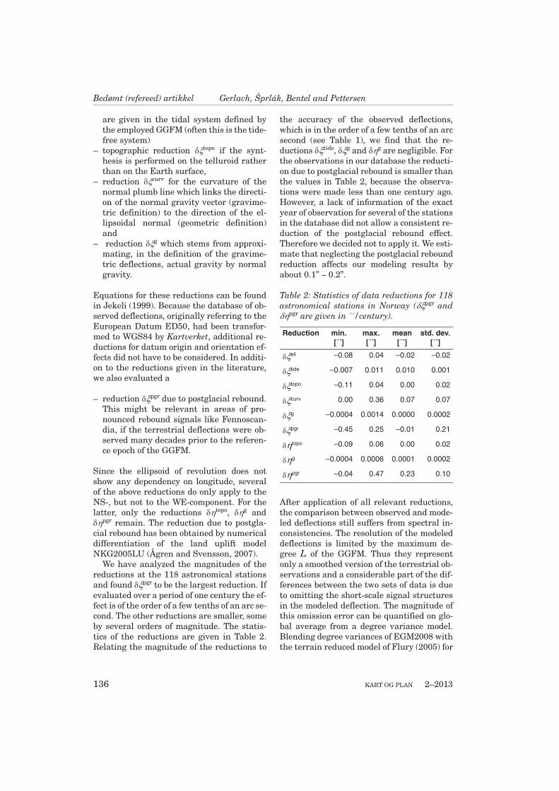
in total. Table 1 shows the mean standarddeviations obtained with each instrumenttype. The magnitude of the deflections ofthe vertical is in the order of ±20“ with amean variation of about 5“. Figure 2 showsthe geographical distribution of the obser-ving stations as well as the deflections (in-dicated by arrows) against the backgroundof the EGM2008 quasi-geoid. EGM2008 is acombined global model (satellite and terres-trial data) of ultra-high maximum sphericalharmonic degree.
Figure 2: The total deflection of the vertical at 118 stations in Norway against the backgroundof the EGM2008 quasi-geoid model.

Observasjon validering, modellering – historiske linjer og nye resultater
KART OG PLAN 2–2013 135
Table 1: Mean standard deviations for different types of astronomical instruments for thesouth-north (ξ) and west-east (η) components of the deflection of the vertical.
L=2190, corresponding to a resolution ofabout 10 km (Pavlis et al., 2012). The astro-nomical observations are unevenly distribu-ted over Norway. The majority of points arelocated along the coast of southern Norway.After identifying and removing eight outliersfrom the database of deflections, the remai-
ning 110 stations were used in the followinganalysis.
Validation methodologyThe north-south (NS) and west-east (WE)component of the deflections of the verticalcan be computed from a GGFM according to
(3)
Evaluation of these equations using thespherical coordinates of the observing sta-tions allows mutual comparison with the ob-served deflections. The latter are derived bycomparing the ellipsoidal coordinates (ϕ,λ) ofthe station with the astronomical ones (Γ,Λ)
(4)
Two aspects are important for the compari-son:
– Definition of the vertical deflections. Ob-served deflections are defined as the diffe-rence between astronomical and ellipsoi-dal coordinates. This definition is referredto as Helmert’s definition (Jekeli, 1999)with geometrical meaning (the physicalplumb line is related to the ellipsoidal nor-mal). In contrast, deflections derived froma GGFM have a gravimetric meaning (theellipsoidal normal is replaced by the direc-tion of the normal gravity vector). Re-ductions need to be applied to relate thetwo definitions.
– Spectral content of the vertical deflections.Observed deflections contain all frequen-cies of the Earth’s gravity field up to infi-
nity. Their modeled counterpart, however,is restricted to the maximum d/o of the em-ployed GGFM. In order to make the spec-tral content consistent, either the observa-tions need to be filtered or the missinghigh frequencies of the modeled deflec-tions need to be reconstructed from additi-onal data. We follow the second option,which is known as the spectral enhance-ment method (SEM) and is explained la-ter.
Following Jekeli (1999), several reductionsneed to be applied to the modeled deflectionsto make them comparable to the observed de-flections. These are, assuming that the mo-deling is based on standard harmonic expan-sions in spherical approximation on the sur-face of the telluroid in the tide-free system:
– ellipsoidal reduction δξell because the mo-deled deflections are based on sphericalapproximation and thus are orientedalong the geocentric radius vector ratherthan along the ellipsoidal normal,
– permanent tidal reduction δξtide to takecare of the fact that the observed deflec-tions are given in the mean permanent ti-dal system, while the modeled coefficients
Transit instrument T4 T2 Zenith camera
Std.dev. (ξ) 0.18“ 0.23“ 0.44“ 0.15“
Std.dev. (η) 0.24“ 0.08“ 0.44“ 0.18“
( )
( )
ϕξ λ λϕ
η λ λ ϕϕ
= =
= =
∂= − Δ + Δ
∂
= − Δ − Δ
0 0
0 0
(sin )( ) cos sin
1( ) cos sin (sin ).
cos
L llm P
GGFM lm P lm Pl m
L l
GGFM lm P lm P lm Pl mP
PP C m S m
P m S m C m P
( )
( )
( ) cos .astro P P
astro P P P
P
P
ξ ϕη λ ϕ
= Φ −= Λ −
Bedømt (refereed) artikkel Gerlach, Šprlák, Bentel and Pettersen
136 KART OG PLAN 2–2013
are given in the tidal system defined bythe employed GGFM (often this is the tide-free system)
– topographic reduction δξtopo if the synt-hesis is performed on the telluroid ratherthan on the Earth surface,
– reduction δξcurv for the curvature of thenormal plumb line which links the directi-on of the normal gravity vector (gravime-tric definition) to the direction of the el-lipsoidal normal (geometric definition)and
– reduction δξg which stems from approxi-mating, in the definition of the gravime-tric deflections, actual gravity by normalgravity.
Equations for these reductions can be foundin Jekeli (1999). Because the database of ob-served deflections, originally referring to theEuropean Datum ED50, had been transfor-med to WGS84 by Kartverket, additional re-ductions for datum origin and orientation ef-fects did not have to be considered. In additi-on to the reductions given in the literature,we also evaluated a
– reduction δξpgr due to postglacial rebound.This might be relevant in areas of pro-nounced rebound signals like Fennoscan-dia, if the terrestrial deflections were ob-served many decades prior to the referen-ce epoch of the GGFM.
Since the ellipsoid of revolution does notshow any dependency on longitude, severalof the above reductions do only apply to theNS-, but not to the WE-component. For thelatter, only the reductions δηtopo, δηg andδηpgr remain. The reduction due to postgla-cial rebound has been obtained by numericaldifferentiation of the land uplift modelNKG2005LU (Ågren and Svensson, 2007).
We have analyzed the magnitudes of thereductions at the 118 astronomical stationsand found δξpgr to be the largest reduction. Ifevaluated over a period of one century the ef-fect is of the order of a few tenths of an arc se-cond. The other reductions are smaller, someby several orders of magnitude. The statis-tics of the reductions are given in Table 2.Relating the magnitude of the reductions to
the accuracy of the observed deflections,which is in the order of a few tenths of an arcsecond (see Table 1), we find that the re-ductions δξtide, δξg and δηg are negligible. Forthe observations in our database the reducti-on due to postglacial rebound is smaller thanthe values in Table 2, because the observa-tions were made less than one century ago.However, a lack of information of the exactyear of observation for several of the stationsin the database did not allow a consistent re-duction of the postglacial rebound effect.Therefore we decided not to apply it. We esti-mate that neglecting the postglacial reboundreduction affects our modeling results byabout 0.1” – 0.2”.
Table 2: Statistics of data reductions for 118astronomical stations in Norway (δξpgr andδηpgr are given in ´´/century).
After application of all relevant reductions,the comparison between observed and mode-led deflections still suffers from spectral in-consistencies. The resolution of the modeleddeflections is limited by the maximum de-gree L of the GGFM. Thus they representonly a smoothed version of the terrestrial ob-servations and a considerable part of the dif-ferences between the two sets of data is dueto omitting the short-scale signal structuresin the modeled deflection. The magnitude ofthis omission error can be quantified on glo-bal average from a degree variance model.Blending degree variances of EGM2008 withthe terrain reduced model of Flury (2005) for
Reduction min.[´´]
max.[´´]
mean[´´]
std. dev.[´´]
δξell –0.08 0.04 –0.02 –0.02
δξtide –0.007 0.011 0.010 0.001
δξtopo –0.11 0.04 0.00 0.02
δξcurv 0.00 0.36 0.07 0.07
δξg –0.0004 0.0014 0.0000 0.0002
δξpgr –0.45 0.25 –0.01 0.21
δηtopo –0.09 0.06 0.00 0.02
δηg –0.0004 0.0006 0.0001 0.0002
δηpgr –0.04 0.47 0.23 0.10

Observasjon validering, modellering – historiske linjer og nye resultater
KART OG PLAN 2–2013 137
the ultra-high degrees, we find an omissionerror of about 3” above the resolution ofGOCE GGFMs, which is not negligible (om-ission errors in rough terrain will be evenlarger than this global average). In order toovercome the spectral inconsistency we try toreconstruct the omitted signal by the spec-tral enhancement method (SEM). The princi-ple is depicted in Figure 3. Thereby the spec-trum is separated into three degree bands,the low to medium degrees, the high degreesand the ultra-high degrees. The low to medi-um degrees are computed from the GGFMunder investigation. In our case this is one ofthe GOCE-based GGFMs. The high degreesabove the resolution of GOCE are recon-structed from EGM2008. The ultra-high de-grees above the resolution of EGM2008, i.e.above d/o 2190, still amount to an omissionerror in the order of 0.4” on global average.Because these short scale structures of thegravity field are strongly correlated to the to-pographic masses, they can be modeled to alarge extent from a digital elevation model(DEM). Therefore a residual terrain model(RTM; Forsberg, 1984) is formed as the diffe-rence between an ultra-high resolution DEMand a smooth topography with a resolutioncorresponding to EGM2008 (this is becauseEGM2008 represents all structures belowdegree 2190, i.e. also the gravity effect of asmooth topography). The ultra-high frequen-cy band is therefore taken care of by directevaluation of the gravitational attractioncaused by the masses within the RTM. Wewant to remind here that the aim of applyingSEM is not to construct the best possible gra-vity field (in this case one would choose aGRACE based model for the low frequenciesinstead of GOCE and not simply glue the dif-ferent spectral bands together), but to vali-date GOCE based GGFMs which requires totake care of their limited spatial resolution.Adding the short scale signal components byapplying SEM is the computationally simp-lest approach to do so.
The SEM strategy has become attractivewith the release of high-resolution GGFMs,such as GPM98A, B (Wenzel, 1998), EGM2008(Pavlis et al., 2012) or EIGEN-6C (Förste etal., 2011). It has been used to recover variousfunctionals of the disturbing potential, i.e.
height anomalies (Hirt et al., 2010), geoidundulations (Gruber et al., 2011), deflec-tions of the vertical (Hirt, 2010; Hirt et al.,2011), gravity disturbances (Hirt et al.,2011), gravity anomalies (Kadlec, 2011;Šprlák et al., 2012), and second order radialderivatives of the disturbing potential(Kadlec, 2011).
We have applied the SEM at all stations ofour deflection database. The harmonic synt-hesis was performed with the GRAFIM soft-ware (Janák and Šprlák, 2006) using thelow- to medium –resolution GOCE models aswell as the high-resolution model EGM2008.Numerical problems of the high degree andorder spherical harmonics have been avoidedby implementing Horner’s scheme (Holmesand Featherstone, 2002) in the GRAFIMsoftware.
Above the resolution of EGM2008, RTMcontributions have been added. The RTMwas obtained as the difference between thehigh resolution DEMs ACE2 (Berry et al.,2010) and ASTER (Tachikawa et al., 2011)and a smooth topography, computed from to-pographical spherical harmonic coefficientsof the elevation model DTM2006.0 (Pavlis etal., 2007). The RTM contributions to the de-flections have been evaluated at each stationby numerical integration. Thereby we haveassumed planar approximation of the cor-responding kernels. To reduce the computa-tional time, the numerical integration hasbeen divided into two zones, an inner and anouter zone. The inner zone makes use of 1´´ ×1´´ discretization of the mass elements asprovided by the ASTER DEM. Such discreti-zation has been applied within the integrati-on radius ψ = 0.1°. Beyond that, the outer in-tegration zone makes use of 30´´ × 30´´discretization of the mass elements as provi-ded by the ACE2 DEM within the integrati-on radius ψ = 0.5°. Numerical experimentsusing variable maximum radii showed thatthe contribution beyond 0.5° is negligible.Throughout the numerical experiments, astandard rock density of 2670 kg m–3 wasused for the topographic masses. The magni-tude of the RTM-effect is estimated by com-parison of the observations with deflectionsmodeled from EGM2008 with and withoutadding the RTM-effect. The statistics are

Bedømt (refereed) artikkel Gerlach, Šprlák, Bentel and Pettersen
138 KART OG PLAN 2–2013
shown in Table 3. The mean value roughlyfits to the global average of 0.4” mentionedabove. The standard deviation of the diffe-rences is reduced by almost 40% when inclu-ding the RTM-effect, which compares nicelyto the results by Hirt (2010) for Germanyand Switzerland.
ResultsIn this section we present the results of ourGOCE validation, i.e. the differences bet-ween observed deflections of the vertical andtheir modeled counterparts. In accordancewith the SEM approach, the modeled deflec-tions are based on a GOCE model up to a cer-tain spherical harmonic degree lmax and thecontribution of EGM2008 and a RTM abovelmax. In order to study the quality of differentspectral bands as well as the effective resolu-tion of the GOCE models, lmax was successi-vely changed from degree 2 up to the maxi-mum degree L of each of the tested models.Figure 4 shows the standard deviations ofthe differences between observed and mode-led deflections computed at all of the 110 sta-tions as function of the maximum d/o lmax ofthe tested model. For example, the value of
the depicted curves at degree 100 is the stan-dard deviation of the differences which isfound, when employing a specific GOCE mo-del up to degree lmax = 100 and EGM2008above degree 101. A smaller standard devia-tion implies better quality of the GOCE mo-del.
In order not to overload the comparisonwith too many almost identical results, werestrict to some few GOCE-based models on-ly, and relate GOCE to independent datasources by adding some GOCE-free models.The following models are considered for thecomparison: EGM96 (state-of-the-art combi-nation model before GRACE/GOCE), ITG-GRACE2010s (probably the best availablepure GRACE model), the GOCE/GRACEcombinations GOCO01s and GOCO03s (bas-ed on ITG-GRACE2010s and the time-wisesolutions of first and third release), and thefirst and third release models of the directmethod (DIR_r1 and DIR_r3).
The differences shown in Figure 4 aremainly caused by errors in the employed mo-dels. Errors of astronomical observations arealmost one order of magnitude smaller. Themodel errors are largest at the higher frequ-
Figure 3: Schema of the spectral enhancement method (SEM).
Table 3: Statistics of the differences between observed and modeled deflections of the verticalat 110 astronomical stations in Norway (with and without consideration of the RTM-effect).
RTM Component min.[´´]
max.[´´]
mean[´´]
std. dev.[´´]
Not includedξ –5.60 9.27 –0.35 2.02
η –9.17 8.00 –0.76 2.39
Includedξ –3.44 4.40 –0.33 1.22
η –4.10 3.58 –0.60 1.54

Observasjon validering, modellering – historiske linjer og nye resultater
KART OG PLAN 2–2013 139
encies. Therefore the total model error bud-get is dominated by errors of EGM2008.Using only EGM2008 for all degrees provi-des a benchmark test which is representedby the black horizontal line in Figure 4. Thestandard deviation of this benchmark scena-rio for the SN-component (top panel) is about1.20´´. The WE-component is at 1.47”, i.e.,the quality of the WE component is about20% worse than the SN component. Replaci-ng EGM2008 in the low- to medium spectralband by any of the other GGFMs under in-vestigation, results in deviations from the
benchmark line. Lower values, i.e. curves be-low the benchmark line, indicate quality im-provement. The spectral/spatial resolution ofthe GGFMs can be defined by the maximumd/o of the model. The effective resolution,however, is given by a signal-to-noise ratio(SNR) of 1. All degrees above the effective re-solution have a smaller SNR value, i.e., theycontain mostly noise. This is clearly shown inFigure 4 by the fact that – above a certain de-gree – all curves start to deviate stronglyfrom the benchmark line. In the sequel allcurves are described in detail.
Figure 4: Standard deviation of the difference between observed and modeled deflections ofthe vertical for varying maximum degree lmax of the employed global gravity field models for(a) south-north and (b) west-east component.

Bedømt (refereed) artikkel Gerlach, Šprlák, Bentel and Pettersen
140 KART OG PLAN 2–2013
EGM96 is the oldest model in our compari-son. It contains satellite tracking data of va-rious satellites acquired over several decadesas well as terrestrial gravity anomalies. Be-low degree 50 there are only slight devia-tions from the benchmark line. Above thisdegree the standard deviations increasestrongly for the NS-component and a bit lesspronounced for the WE-component. After ap-proximately degree 120 the error level staysalmost constant. The lower degrees are do-minated by the old satellite tracking dataand also by the global average quality of ter-restrial data. Higher degrees, in tendency,are more dependent on the regional qualityof the terrestrial data. The constant error le-vel above degree 120 indicates that, for thehigher degrees, the error level of EGM96 isnot significantly worse than for EGM2008.Indeed EGM2008 builds upon the same ter-restrial database that was already used inEGM96 (Pavlis et al., 2012). It is alsoworthwhile to note, that the quality of thedegrees below 30–50 cannot be judged fromthe representation in Figure 4. This is becau-se the error budget is dominated by the high-er frequencies and even significantly smallererror contributions in the low frequenciescannot change the overall error budget. The-refore one cannot recognize the tremendousincrease in quality of the satellite-only solu-tions of GOCE and especially of GRACE ascompared to the older satellite-tracking data.
The standard deviations of the NS-compo-nents for all GRACE and GOCE-based mo-dels reveal an improvement in the low andmid frequency range around degrees 110-160. Beyond this point the standard devia-tions of the satellite models increase by seve-ral tenths of an arc second. For ITG-GRACE2010s a significant increase at d/o160–180 is evident while the GOCE modelsare significantly better in this frequency ran-ge (Gruber et al., 2011; Hirt et al., 2011). It isalso interesting to note the different behavi-or of the NS- and the WE-components of ITG-GRACE2010s above degree 140. While theNS-deflection deviates only slightly from thebenchmark line up to degree 160 and diver-ges strongly thereafter, the WE-deflectionstarts deviating already around degree 140,but does not diverge that significantly. This
might be related to the error characteristicsof the GRACE mission with its significantstriping pattern in NS-direction (i.e., alongthe orbit tracks). This pattern is related topronounced error correlations in NS-directi-on. Because the deflections of the vertical re-present derivatives of the geoid in NS- andWE- direction, the error correlations directlyinfluence the error budget of the deflections.Larger correlations in one direction implysmaller error estimates for the correspon-ding directional derivatives. Therefore onemay expect the NS-error to be smaller thanthe WE-error due to much larger correlationlengths in NS-direction. This could explainthe smaller error budget of the NS-compo-nent up to degrees around 160.
It is also interesting to note, that only twomonths of GOCE data (release 1) already im-prove solutions from seven years of GRACEdata in the medium frequencies. This is morepronounced in the WE-component whereGOCO01s significantly deviates from ITG-GRACE2010s.
As expected, the increase of the standarddeviations of all GOCE models at higher fre-quencies depends on the release number. Ge-nerally, higher release number means moredata and therefore better performance athigher frequencies. This is nicely illustratedby the NS-component of the GOCO models,where release 1 starts diverging at arounddegrees 160–170, while release 3 (with al-most eight times more data than release 1)does not diverge before degree 220.
An important test for quality assessmentof HPF’s processing chain is to compareGOCE models based on different analysisstrategies. Comparing the release 3 modelsof GOCO (based on the time-wise approach)and the direct approach, we see very similarerror behavior. This indicates a high qualityof the processing chain independent on theanalysis strategy. This also confirms the re-sults of previous studies and is in very goodagreement with Šprlák et al. (2012). Theore-tically, all three analysis strategies may beassumed to provide identical results. Thequality of the different solutions and the dif-ferences between them thus depends crucial-ly on the filtering of observations and the useof a priori information. This is evident from

Observasjon validering, modellering – historiske linjer og nye resultater
KART OG PLAN 2–2013 141
the first release of the direct approach, whichshows an exceptionally good behavior evenup to the highest degrees. This is also foundin the studies by Janák and Pito ák (2011),Tscherning and Arabelos (2011), Voigt andDenker (2011) and Šprlák et al. (2012). It canbe explained by the fact that DIR_r1 uses thecombined model EIGEN-GL5C (Förste et al.,2008) as a priori information. The terrestrialgravity data in the a priori model causes thelow error budget and prevents the error cur-ve from diverging from the benchmark line.After recognizing the strong correlation ofthe final GOCE-DIR model with prior infor-mation, the satellite-only model ITG-GRACE2010s was introduced as a priori gra-vity field model. This prevents terrestrialgravity data from affecting the solution. Thesecond release of the direct approach wasused as a priori model for the estimation ofthe third release direct model DIR_r3. Thisshows the importance of the proper choice ofprior information and that a reasonable choi-ce of a priori information in the direct met-hod leads to a competitive performance withrespect to the time-wise solution. It shouldbe mentioned that integration of a priori in-formation is in the time-wise models limitedto regularization of the high frequencies ofthe spectra above degree 180 applying Kau-la’s degree variance model (Kaula, 1966). Thisgives a rough estimate of the expected avera-ge size of spherical harmonic coefficients of acertain degree and helps to smooth the noisecontribution in the high frequencies.
Overall, the level of improvement broughtby different releases of GOCE models is appro-ximately equal for both the SN and the WEcomponent. However, the level is four timessmaller than reported by Voigt and Denker(2011) and two times smaller than observed byŠprlák et al. (2012). The discrepancies with re-spect to Voigt and Denker (2011), who perfor-med their study with deflections of the verticalin Germany, might be caused by the differentgeographic locations of the study area (see e.g.Šprlák et al., 2012). The less pronounced im-provements with respect to (Šprlák et al.,2012), who validated GOCE models over Nor-way using gravity anomalies, might be causedby different spectral characteristics of diffe-rent gravity field functionals.
Regional modeling of the gravity fieldMany geodetic applications require high re-solution gravity field information. Therefore,regional refinements of global models – suchas those derived from GOCE – are necessary.Classical techniques for such a regional gra-vity field modeling are the integration of ter-restrial gravity anomalies by means of Sto-kes’s equation
(5)
and least-squares collocation, which provi-des an optimal estimation of arbitrary gravi-ty field quantities from various point obser-vations in a statistical sense. It employsknowledge of the signal covariance and triesto minimize the prediction error. If we re-strict ourselves to a comparison with Sto-kes’s equation, i.e. with the estimation of ge-oid heights from gravity anomalies, collocati-on can be written in the following way
(6)
where matrices C contain signal covariancesbetween the functionals indicated in the su-perindex at locations indicated in the index;in that sense represent cross-covarian-ces between gravity anomalies and geoidheights between the points i of the inputdata and computation point P.
Both methods can be applied globally.However, due to the large number of gravitypoints available, collocation requires hugecomputational efforts when applied to largerdata sets. In practice both methods are appliedregionally and only the residual geoid with re-spect to a long wavelength reference model isapproximated. In the case of Stokes the globalmodel is necessary because equation (5) requi-res global integration, which for the largestsignal contribution is implicitly included inthe reference model. In case of collocation, thestatistical setup requires the residual signal tobe of stochastic nature without deterministiccomponents such as trends or periodic oscilla-tions. Such deterministic components are re-duced by computation of residual quantities.The use of global reference models also allows
( ) ( ) d4 PQ Q Q
RN P S g
σ
ψ σπγ
= Δ
( )−= Δ
1( ) ,Ng gg
Pi ij iN P C C g
NgPiC

Bedømt (refereed) artikkel Gerlach, Šprlák, Bentel and Pettersen
142 KART OG PLAN 2–2013
restricting the use of terrestrial data to a limi-ted region. Usually the reference models areprovided in terms of spherical harmonics.From a set of spherical harmonic coefficients
of the disturbing potential, the ge-oid can be computed according to
(7)
All of the three classical methods/paramete-rizations (equations (5)–(7)) are identical ifapplied globally. This holds true for Stokes’sintegral and the spherical harmonic repre-sentation (see Heiskanen and Moritz, 1967),but may also be shown for Stokes integraland collocation. Following the interpretationin de Min (1995), the gravity anomalies usedin Stokes’s integral (integration elements atpoint Q) are predicted from point gravity va-lues observed at discrete location i by meansof collocation. Then Stokes’s equation can bewritten as
(8)
and because the original gravity stations i donot depend on the integration element
(9)
Both of the functions inside of the integralcan be written in terms of Legendre series,i.e.
(10)
(11)
with cl being the signal degree variancesof the residual gravity anomalies and
are the Legendre polynomials.Insertion of equation (10) and (11) into (9)and application of decomposition theoremand orthogonality relations of spherical har-monics (see Heiskanen and Moritz, 1967)yields
·
(12)
This derivation shows that Stokes integraland collocation are identical, if applied global-ly. Thereby, collocation is interpreted as a twostep procedure. In the first step gravity ano-malies are predicted continuously over the en-tire Earth’s surface from given point gravitydata in the area of interest. In the second stepStokes’s integration of this continuous dataset of predicted gravity anomalies is perfor-med globally. However, de Min (1995) pointsout that the two methods are not identical inregional applications. This is because Stokes’sintegration can easily be restricted to a sphe-rical cap around the computation point (withno data from outside the cap being used), whi-le collocation implicitly takes the contributionfrom outside the cap into account. Thishowever is not desired because the data in thefar zone does not reflect the actual gravityfield outside the cap, but is only derived by ex-trapolation of the data inside the cap. Theproblem can be overcome by proper modifica-tion of the cross-covariance function CNg
(which is equivalent to a modification of theStokes kernel) such that both methods beco-me identical.
Besides these classical methods sphericalwavelet representations – or generally the useof spherical radial basis functions – have beco-me popular since several years, see e.g.Freeden and Schreiner (2005), Panet et al.
{ },lm lmC SΔ Δ
( λ= =
= Δ + Δ2 0
( ) cosL l
lm Pl m
N P R C m
)λ θΔ sin (cos ).lm P lm PS m P
( ) 1
( ) ( ) d4
( ) d4
PQ Q Q
gg ggPQ Qi ij i Q
RN P S g
RS C C g
σ
σ
ψ σπγ
ψ σπγ
−
= Δ
= Δ
( )σ
ψ σπγ
−= Δ
1( ) ( ) d .
4gg ggQi Q ij i
RN P S C C g
( )2
2 1( ) cos
1PQ l PQl
lS P
lψ ψ
∞
=
+=−
( )2
cos ,ggQi l l Qi
l
C c P ψ∞
=
=
( )cosl QiP ψ
( )σ
ψπγ
∞
=
+=−2
2 1cos
4 1 l PQl
R lN P
l
( ) ( )ψ σ∞ −
=
Δ1
2
cos d ggl l Qi Q ij i
l
c P C g
( ) ( )
( )
ψγ
∞ −
=
−
= Δ−
= Δ
1
2
1
cos( 1)
.
ggl l Pi ij i
l
Ng ggPi ij i
Rc P C g
l
C C g

Observasjon validering, modellering – historiske linjer og nye resultater
KART OG PLAN 2–2013 143
(2005), Schmidt et al. (2007), Tenzer and Klees(2007) or Antoni et al. (2009). Such approachescan be interpreted as spectral representations(based on spherical harmonics) which are limi-ted to a certain spatial region only. Similar tothe signal covariance functions used in colloca-tion, the radial basis functions depend on aspecific location (origin) and the spherical dis-tance between this origin and the actual com-putation point. In contrast, the spherical har-monic basis functions and
only depend on the compu-tation point P. This is reflected in the amplitu-de of the oscillations of the basis functions,which are shown in Figure 5. The amplitude isconstant all around the globe in the case of sp-herical harmonics (mid panel in Figure 5). Inthe case of radial basis functions (right panelin Figure 5) the amplitude is strongly diminis-hed with increasing distance from the origin.Therefore the influence of a radial basis functi-on on very distant points is practically zero,which makes them suitable for regional gravi-ty field modeling. One says that spherical har-
monics have global support, while radial basisfunctions have quasi4 local support. Sphericalharmonics, which have global support in thespatial domain, are related to one single com-bination of degree and order numbers {l,m}, i.e.they are related to exactly one spectral line andtherefore are perfectly localizing in the spec-tral domain. Perfect localization in either thespectral or the spatial domain goes hand-in-hand with no localization in the other domain.Perfect localization in both domains is not pos-sible. Spherical harmonics are an extremeexample of having perfect frequency localizati-on, but no spatial localization. The other extre-me, no frequency localization but perfect spati-al localization is given by the Dirac-functionwith infinite amplitude at the origin and zeroamplitude at all other locations. Wavelets orradial basis functions represent a compromise.They are quasi-localizing in the spatial domainat the cost of spreading the spectral contentover a wider range of spectral lines, or spheri-cal harmonic degrees (see Figure 6).
Independent of their localization properties,it can be shown that representations in sphe-rical harmonics and in radial basis functionsare mathematically equivalent – at least ifthe latter are distributed evenly around theglobe. This is shown in the following equa-tions. For the sake of compactness of theequations, we use complex notation for sphe-
rical harmonics with the order number m co-vering all degrees in the range {–l; l} and
(cos )coslm P PP mθ λ(cos )sinlm P PP mθ λ
4. The amplitude is very small for large distances from the origin, but not exactly zero. Therefore the support is not actually local, but only quasi-local.
Figure 5: The global geoid (left) can be constructed from a superposition of spherical harmonic ba-sis functions (middle) or of quasi space localizing radial basis functions (right). The middle panelshows a tesseral spherical harmonic function of degree l=8 and order m=4. The right panel showsa Blackman scaling function located at the origin with spherical coordinates λ=30° and ϕ=55°.
( ) cos1cos
sin4PR
lm Pl mP
mY P
mR
λθ
λπ= ⋅
0,...,for
,..., 1l
ml
=− −

Bedømt (refereed) artikkel Gerlach, Šprlák, Bentel and Pettersen
144 KART OG PLAN 2–2013
In this notation, the spherical harmonic seri-es expression of the gravitational potential(cf. equation (1)) is given by
(13)
Thereby the spectral coefficients clm may bederived by spherical harmonic analysis, i.e.from the global integration of the productbetween signal (the potential function V gi-ven at points Q on the surface of the sphere)and the basis function of the correspon-ding degree and order numbers l and m. In-serting this into equation (13) yields
· , (14)
and after interchanging the order of summa-tion and integration and employing the addi-tion theorem of spherical harmonics (seeHeiskanen and Moritz, 1967)
·
· (15)
Introducing the Abel-Poisson kernel function
(16)
we may write
(17)
This is a convolution of the potential V, givenat the surface of the sphere (at points Q) withthe kernel function kAP(P,Q) between pointsP and Q. In symbolic notation the convoluti-on can be written as
(18)
The derivation shows, that convolution witha proper kernel function is equivalent to thespherical harmonic representation of equati-on (13). The convolution formula (17) is alsoequivalent to the well known Poisson inte-gral (Heiskanen and Moritz, 1967)
(19)
where s is the distance between points P and
Q, i.e. .
It is important to note that convolution withthe Abel-Poisson kernel kAP gives the origi-nal signal. The kernel is a reproducing ker-nel. There is a wide range of kernels whichhave interesting properties for regional gra-vity field modeling. Generalizing the repre-sentation of the Abel-Poisson kernel in equa-tion (16), we may write the general kernelfunction B(P,Q) as
(20)
where the coefficients Bl define the characte-ristics of the kernel function. All kernel func-tions of this type are isotropic functions, be-cause they depend only on the spherical dis-tance ψPQ between the points P and Q. Thusthey are called radial basis functions. Com-parison of equations (16) and (20) shows thatBl = 1 for all degrees l of the Abel-Poissonkernel. Modification of the Bl-coefficientschanges the spectral characteristics as well
π= ⋅ =− −0,...,
4 for .,..., 1
lmlm
lm
C lc GM m
lS
( )1
0
( ).l
lR
lm lml m lP
RV P c Y P
r
+∞
= = −
=
RlmY
( )+∞
=
=1
0
l
l P
RV P
r
= − Ω
Ω( ) ( ) ( )Q
lR R
lm Q lmm l
V Q Y Q d Y P
( )1
0
( )Q
l
l P
RV P V Q
r
+∞
=Ω
=
( ) ( ) dl
R Rlm lm Q
m l
Y Q Y P= −
⋅ Ω
1
0
( )Q
l
l P
RV Q
r
+∞
=Ω
=
( )2
2 1cos d .
4 l PQ Q
lP
Rψ
π+ Ω
1
20
2 1( , ) (cos )
4
l
AP l PQl
l Rk P Q P
R rψ
π
+∞
=
+=
( ) ( ), ( ) d .Q
AP QV P k P Q V QΩ
= Ω
( ) ( )( ) .Q
AP PV P k V xΩ
= ∗
( )2 2
3
( )( ) d
4Q
PQ
R r RV P V Q
sπΩ
−= Ω
2 2 2 cosP P PQs r R Rr ψ= + −
ψπ
+∞
=
+=1
20
2 1( , ) (cos ),
4
l
l l PQl
l RB P Q B P
R r

Observasjon validering, modellering – historiske linjer og nye resultater
KART OG PLAN 2–2013 145
as the spatial shape of the kernel function.Several radial basis functions as well as thecorresponding Bl-coefficients are shown inFigure 6. The spectral representation reve-als that the modification of the Bl-coeffici-ents corresponds to signal filtering. Therebylow-pass (right column in Figure 6) andband-pass (left column) filtering is possible.In connection with wavelet theory, band-passfiltering is provided by wavelet functions,which cover only a certain spectral band.Low-pass filtering is provided by scalingfunctions, which represent the superposition
of wavelets from different spectral bands.The examples shown in Figure 6 cover sca-ling and wavelet functions of type Shannon,Blackman and Poisson multipole as well as acubic polynomial and the Abel-Poisson ker-nel. They have been discussed in Freeden etal. (1998), Freeden and Michel (2004), Hol-schneider et al. (2003), Chambodut et al.(2005), Panet et al. (2005), Schmidt et al.(2006), Schmidt et al. (2007), Tenzer and Kle-es (2007), Eicker (2008), Klees et al. (2008),Antoni et al. (2009) and Panet et al. (2010)amongst many others.
The spatial characteristics in the upperrow of Figure 6 show that all of the basisfunctions oscillate around zero, have the lar-gest amplitude at the origin and drop to rela-tively small values with increasing distancefrom the origin. This is similar to collocation,where the signal covariance function has thelargest amplitude at the origin (the signalvariance) and drops towards zero for increa-sing distance. Therefore, in both cases, datapoints near the origin have the strongest in-fluence on the modeling result, while data inremote zones play a minor role. However, re-stricting gravity field modeling to local or re-gional scales still leads to truncation errors,
which cannot be avoided, and which aremore or less significant depending on thesize of the study area, the spectral characte-ristics of the signal as well as on the chosenbasis function.
Most of the functions in Figure 6 show asmooth transition in the spectral domain (lo-wer panels) from values of one to zero. Onlythe Shannon wavelet (band-pass) shows asharp transition. It exactly (and completely)cuts a certain band from the spherical har-monic degree spectrum. Therefore, in a glo-bal gravity field representation, a band-limi-ted signal can be exactly represented withthe Shannon wavelet, provided that the mi-
Sp
ectra
l
S
patia
l
dom
ain
dom
ain
• 4 • 3 • 2 • 1 0 1 2 3 4
0
0.5
1
spherical distance (deg)
50 100 150 200 250 300 350 400 450 5000
0.5
1
sh degrees (n)
• 4 • 3 • 2 • 1 0 1 2 3 4
0
0.5
1
spherical distance (deg)
100 200 300 400 5000
0.5
1
sh degrees (n)
Figure 6: Spatial (upper panels) and spectral (lower panels) representation of different typesof band-pass (wavelet) and low-pass (scaling) functions.

Bedømt (refereed) artikkel Gerlach, Šprlák, Bentel and Pettersen
146 KART OG PLAN 2–2013
nimum and maximum degree of the Shan-non wavelet coincides with the minimumand maximum degree of the signal. As shownin equation (17), convolution with the Abel-Poisson kernel reproduces the non band-li-mited gravity signal exactly. However, convo-lution requires a continuous and completecoverage of and integration over the wholeglobe. Because this is numerically not pos-sible, there is an approximation error.Furthermore, truncation errors arise fromrestricting the computations to local or regi-onal scales, as discussed above. Additionally,if we assume a gravity signal in the band-width from, e.g., spherical harmonic degree150 to 250 (this corresponds to the pass-bandof the Shannon wavelet in Figure 6), not allof the radial basis functions presented in Fi-gure 6 can reproduce the full spectral con-tent of the signal due to their spectral cha-racteristics (limited frequency localization).But because the radial basis functions are acompromise between localization in the spa-tial and spectral domain, making only use ofthe spectral characteristics for assessment ofthe modeling quality is not advisable. In-deed, validations of modeling results showthat functions which are smooth both in thespatial and frequency domains lead to bettermodeling results than, e.g., the Shannonband-pass function. Even though the latterexactly covers the signal bandwidth in thespectral domain, it has the highest side-lobesand oscillations in the spatial domain whichis unfavorable considering space-localizingrequirements in regional modeling.
In the sequel we present a synthetic exam-ple of regional gravity field modeling. There-by a closed-loop model is set up to test thequality of regional modeling. In the first step(estimation), synthetic data is generatedfrom a spherical harmonic input model andused to derive a regional gravity field model.In the second step (validation) the regionalfield is compared to values derived from theinput model at an independent set of valida-tion points. The difference between the tworepresentations is the empirical error of theregional modeling. The linear observationmodel employed in the estimation step is ba-sed upon the following mathematical consi-deration: if two functions are in the same
function space, then the result of their convo-lution is as well in the same space. In our ca-se, the gravitational potential V(Q) and thekernel B(P,Q) are in the linear space of squa-re integrable functions L2 on the sphere.Therefore also the result of the convolutionV · B is in L2 on the sphere and can be repre-sented as linear combination of a set of ker-nel functions B(P,Q) (which span L2), locatedon a regular grid with k grid points Qk cove-ring the area of interest. It holds
(21)
from which the linear observation model
(22)
is derived. Thereby the elements of the de-sign matrix are computed from the kernelfunction and the coefficient vector dk con-tains the unknowns. Given gravity field ob-servations at data points P and the distribu-tion of grid points Qk, the unknown coeffici-ents can be estimated in least-squares sense.This also allows for a proper description ofthe formal error of the dk coefficients and er-ror propagation to arbitrary gravity fieldquantities. The estimation model can be ex-tended to combine different types of observa-tions, like geoid heights, gravity anomalies,gravity gradients in orbit height, etc. In addi-tion, proper selection and/or modification ofthe kernel function allows spectral filtering.
The results of our synthetic example areshown in Figure 7. The Shannon low-passfunction is used for gravity field representati-on. The study area is located in the Himalayaregion between 27° and 33° latitude and 77°and 88° longitude. The signal is shown in theleft panel of Figure 7 and represents the gravi-tational potential in the bandwidth betweenspherical harmonic degrees 150 and 250. Theempirical error of the regional model is shownin the right panel of in Figure 7. The relativeempirical error has an RMS value of only1.2 · 10–5 which corresponds to 12 μm in termsof geoid heights. Using other types of radial
( ) ( )( )Q
PV P B V xΩ
= ∗
1 1
( , ) ( , )K
k k k kk k
d B P Q d B P Q∞
= =
= ≈
( ) ( ) ( , )Tk kP P P Q+ = ⋅y e B d

Observasjon validering, modellering – historiske linjer og nye resultater
KART OG PLAN 2–2013 147
basis functions, this error can be further redu-ced. The cubic polynomial or Poisson multipolekernels yield about two orders of magnitudesmaller errors. The relative empirical errorhas an RMS of the order of 10–7.
It is worthwhile to note, that the sphericalharmonic representation of the signal con-tains 40200 coefficients, while for the regional
representation only 1437 coefficients are nee-ded. Because radial basis functions are onlyrequired in the area of interest (includingsome margin to minimize truncation errors)the number of coefficients used to representthe signal is relatively small. Therefore theyallow very detailed refinements in the area ofinterest with moderate numerical effort.
Summary and conclusionsDrawing historical lines from the beginningof Norwegian gravity field research in the1860ies, current research topics at the Nor-wegian University of Environmental and LifeSciences are presented. We have validatedESA’s satellite gravimetry mission GOCEwith historic astronomical observations inNorway, many of which Olav Mathisen hadmeasured. The comparison shows the highquality of GOCE data products in general,but also reveals differences in processingstrategies. Global gravity field models, likethose based on GOCE, act as long-wave-length reference models for regional refine-ments. Besides the classical methods likeStokes integration and collocation, today, alsospherical wavelet-type representations areinvestigated. We have described the generalconcept and shown that regional modeling ispossible with very high accuracy. Advantagesof representations in radial basis functionsare their spectral form which allows data fil-tering, the quasi-local support which allowsrestriction of the modeling to the region of in-
terest and the formulation in terms of a line-ar observation model. This allows combinati-on of different types of gravity field observa-tions and the derivation of proper error mea-sures. The limitation of the study region ma-kes the estimation efficient and keeps the nu-merical effort on a moderate level.
AcknowledgementsKartverket is gratefully acknowledged forproviding the database of vertical deflectionsin Norway. Michael Schmidt of DGFI in Mu-nich is gratefully acknowledged for discus-sions on radial basis functions. Last but notleast, we thank Olav Mathisen for his conti-nuing and inspiring guidance of studentsand colleagues at UMB.
ReferencesAntoni, M., Keller, W., and Weigelt, M., 2009,
Representation of Regional Gravity Fields byRadial Base Functions. In: Sideris, M.G. (red.)Observing our Changing Earth. IAG Symposia,Vol. 133, 293–299. Springer Berlin Heidelberg.
Figure 7: Gravitational potential in the Himalaya region in the spectral range between sphericalharmonic degrees 150 and 250 (left) and the empirical error (right) of a corresponding regionalgravity field model based on Shannon band-pass basis functions.

Bedømt (refereed) artikkel Gerlach, Šprlák, Bentel and Pettersen
148 KART OG PLAN 2–2013
Berry, P.A.M., Smith, R.G., Benveniste, J., 2010,ACE2: The new global digital elevation model.In: Mertikas S.P. (Ed.), Gravity, Geoid andEarth Observation, IAG Symposia, Vol. 135,23–27 June 2008, Chania, Greece, p. 231–238.
Blankenburgh, J. C., 1987, Geodesi med stjernerog satellitter i Norge. Bilag til Kart og Plan nr.1 – 1987, p. 91–95.
Breili, K., Gjevestad, J. G., Lysaker, D. I., Omang,O. C. D., Pettersen, B. R., 2010, Absolute gravityvalues in Norway. Norwegian Journal of Geo-graphy 64, 79–84.
Bruinsma, S.L., Marty, J. C., Balmino, G., Bianca-le, R., Foerste, C., Abrikosov, O., and Neumayer,H., 2010, GOCE Gravity Field Recovery byMeans of the Direct Numerical Method, presen-ted at the ESA Living Planet Symposium 2010,Bergen, June 27–July 2 2010, Bergen, Norway.
Chambodut, A., Panet, I., Mandea, M., Diament,M., Holschneider, M., and Jamet, O., 2005,Wavelet frames: an alternative to spherical har-monic representation of potential fields. Geop-hysical Journal International, 163, 875–899.
Danielsen, J., Sundsby, J., 1995, Målinger medsenitkamera for loddavvik. Faglig melding,Geodesidivisjonen, Statens kartverk.
Drewes, H., 2012, Current Activities of the Inter-national Association of Geodesy (IAG) as theSuccessor Organisation of the Mitteleuropäis-che Gradmessung. ZfV, 137(3).
ESA, 1999, Gravity Field and Steady-State OceanCirculation Mission. ESA SP-1233(1), report formission selection of the four candidate EarthExplorer missions.
Eicker, A., 2008, Gravity Field Refinement byRadial Basis Functions from In-situ SatelliteData. Dissertation, Institut für Geodäsie undGeoinformation, Universitity Bonn, Germany.
Flury, J., 2005, Short-wavelength Spectral Proper-ties of the Gravity Field from a Range of Regio-nal Data Sets. Journal of Geodesy, 79(10–11),624–640, doi: 10.1007/s00190-005-0011-y.
Forsberg, R., 1984, A study of terrain reductions,density anomalies and geophysical inversionmethods in gravity field modeling. Report No.355, Department of Geodetic Science and Sur-veying, Ohio State University, Columbus, USA.
Förste, C., Bruinsma, S., Shako, R., Marty, J.-C.,Flechtner, F., Abrikosov, O., Dahle, C., Lemoine,J.-M., Neumayer, H., Biancale, R., Barthelmes,F., König, R., and Balmino, G., 2011, EIGEN-6 –A new combined global gravity field model
including GOCE data from the collaboration ofGFZ-Potsdam and GRGS-Toulouse. Geophysi-cal Research Abstracts, Vol. 13, EGU2011-3242-2, EGU General Assembly 2011.
Freeden, W., Gervens, T., and Schreiner, M., 1998,Constructive Approximation on the Sphere WithApplications to Geoscience. Oxford SciencePublications.
Freeden, W., and Michel, V., 2004, MultiscalePotential Theory With Applications to Geoscien-ce. Springer Basel AG.
Freeden, W., and Schreiner, M., 2005, Spacebornegravitational field determination by means oflocally supported wavelets. Journal of Geodesy,79, 431–446.
Gauss, C. F., 1828, Bestimmung des Breitenunter-schiedes zwischen den Sternwarten von Göt-tingen und Altona durch Beobachtungen amRamsdenschen Zenithsector. Vandenhoeck undRuprecht, Göttingen.
Gruber, T., Visser, P.N.A.M., Ackermann, C., Hosse,M., 2011, Validation of GOCE gravity fieldmodels by means of orbit residuals and geoidcomparisons. Journal of Geodesy, 85, p. 845–860.
Guimarãeas, G.N., Matos, A.C.O.C., Blitzkow, D.,2012, An evaluation of recent GOCE geopoten-tial models in Brazil. Journal of Geodetic Scien-ce, 2, p. 144–155.
Hansteen, C., 1825, Capt. Sabines Pendel-Iagttagel-ser. Magazin for Naturvidenskaberne 6, 309–310.
Heiskanen, W., and Moritz, H., 1967, PhysicalGeodesy. Freeman, San Francisco.
Hirt, C., 2010, Prediction of vertical deflectionsfrom high-degree spherical harmonic synthesisand residual terrain model data. Journal ofGeodesy, 84, p. 179–190.
Hirt, C., Featherstone, W.E., Marti, U., 2010, Com-bining EGM2008 and SRTM/DTM2006.0 resi-dual terrain model data to improve quasigeoidcomputations in mountainous areas devoid ofgravity data. Journal of Geodesy, 84, p. 557–567.
Hirt, C., Gruber, T., Featherstone, W.E., 2011, Eva-luation of the first GOCE static gravity fieldmodels using terrestrial gravity, vertical deflec-tions and EGM2008 quasigeoid heights. Jour-nal of Geodesy, 85, p. 723–740.
Holmes, S.A., Featherstone, W.E., 2002, A unifiedapproach to the Clenshaw summation and therecursive computation of very high degree andorder normalized associated Legendre func-tions. Journal of Geodesy, 76, p. 279–299.

Observasjon validering, modellering – historiske linjer og nye resultater
KART OG PLAN 2–2013 149
Holschneider, M., Chambodut, A., and Mandea,M., 2003, From global to regional analysis of themagnetic field on the sphere using wavelet fra-mes. Physics of the Earth and Planetary Interi-ors, 135, 107–124.
Janák, J., Šprlák, M., 2006, A new software forgravity field modeling. Geodetic and Cartograp-hic Horizon, 52, p. 1–8 (in Slovak).
Janák, J., Pito ák, M., 2011, Comparison and testingof GOCE global gravity models in central Europe.Journal of Geodetic Science, 1, p. 333–347.
Jekeli, C., 1999, An analysis of vertical deflectionsderived from high-degree spherical harmonicmodels. Journal of Geodesy, 73, p. 10–22.
Jelstrup, H.J., 1929, Determinations of astronomi-cal longitudes, latitudes and azimuths. Geode-tiske arbeider, hefte II (1929) og III (1931), Nor-ges geografiske opmåling.
Kaula, W., 1966, Theory of satellite geodesy. Blais-dell Pub. Co., Waltham, Massachusetts.
Kadlec, M., 2011, Refining gravity field parame-ters by residual terrain modeling. DoctoralThesis, Department of Mathematics, Faculty ofApplied Sciences, University of West Bohemia,Pilsen, Czech Republic, 150 p.
Klees, R., Tenzer, R., Prutkin, I., and Wittwer, T.,2008, A data-driven approach to local gravityfield modelling using spherical radial basisfunctions. Journal of Geodesy, 82, 457–471.
Koop, R., Visser, P.N.A.M., Tscherning, C.C., 2001,Aspects of GOCE calibration. In: Proceedings ofthe International GOCE User Workshop, WPP-188, ESA/ESTEC, Noordwijk, Netherlands, p.51–56.
Kühnen, F. J., Furtwängler, P., 1906, Bestimmungder absoluten Grösze der Schwerkraft zu Pots-dam mit Reversionspendeln. Veröff. kgl. preuss.geodät. Inst., N.F., Nr. 27.
Listing, J. B., 1873, Über unsere jetzige Kenntnisder Gestalt und Größe der Erde. Nachrichtender Königlichen Gesellschaft der Wissenschaf-ten und der Georg-August-Universität, 33–98,Göttingen.
Lemoine, F.G., Kenyon, S.C., Factor, J.K., Trimmer,R.G., Pavlis, N.K., Chin, D.S., Cox, C.M., Klosko,S.M., Luthcke, S.B., Torrence, M.H., Wang, Y.M.,Williamson, R.G., Pavlis, E.C., Rapp, R.H.,Olson, T.R., 1998. The development of the jointNASA GSFC and NIMA geopotential modelEGM96. NASA Technical Report 1998-206861,NASA/GSFC, Greenbelt, USA.
Mayer-Gürr, T., Rieser, D., Höck, E., Brockmann,J.M., Schuh, W.D., Krasbutter, I., Kusche, J.,Maier, A., Krauss, S., Hausleitner, W., Baur, O.,Jäggi, A., Meyer, U., Prange, L., Pail, R., Fecher,T., Gruber, T., 2012, The new combined satelliteonly model GOCO03s. Abstract submitted toGGHS2012, Venice (Poster).
Migliaccio, F., Reguzzoni, M., Sansó, F., Tscher-ning, C.C., Veicherts, M., 2010, GOCE data ana-lysis: the space-wise approach and the first spa-ce-wise gravity field model. In: Proceedings ofthe ESA Living Planet Symposium, 28 June–2July 2010, Bergen, Norway.
de Min, E., 1995, A comparison of Stokes’s numeri-cal integration and collocation, and a new combi-nation technique. Bull. Géod., 69: 233–232.
Pail, R., Goiginger, H., Schuh, W.D., Höck, E.,Brockmann, J.M., Fecher, T., Gruber, T., Mayer-Gürr, T., Kusche, J., Jäggi, A., Rieser, D., 2010,Combined satellite gravity field modelGOCO01S derived from GOCE and GRACE.Geophysical Research Letters, 37, L20314,doi:10.1029/2010GL044906.
Pail, R., Bruinsma, S., Migliaccio, F., Förste, C., Goi-ginger, H., Schuh, W.D., Höck, E., Reguzzoni, M.,Brockmann, J.M., Abrikosov, O., Veicherts, M.,Fecher, T., Mayrhofer, R., Krasbutter, I., Sansó, F.,Tscherning, C.C., 2011, First GOCE gravity fieldmodels derived by three different approaches.Journal of Geodesy, 85, p. 819–843.
Panet, I., Jamet, O., Diament, M., and Chambod-ut, A., 2005, Modelling the Earth’s gravity fieldusing wavelet frames. In: Jekeli, C., Bastos, L.,Fernandes J. (eds.) Gravity, Geoid and SpaceMissions. IAG Symposia, Vol. 129, pp. 48–53.Springer Berlin Heidelberg.
Panet, I., Kuroishi, Y., and Holschneider, M., 2010,Wavelet modelling of the gravity field bydomain decomposition methods: an exampleover Japan. Geophysical Journal International,184, 203–219.
Pavlis, N.K., Factor, J.K., Holmes, S.A., 2007, Ter-rain-related gravimetric quantities computedfor the next EGM. In: Gravity Field of theEarth, Proceedings of the 1st InternationalSymposium of the International Gravity FieldService, Harita Dergisi, Special Issue 18, Istan-bul, Turkey, p. 318–323.
Pavlis, N. K., Holmes, S. A., Kenyon, S. C., Factor,J. K., 2012, The development and evaluation ofthe Earth Gravitational Model 2008
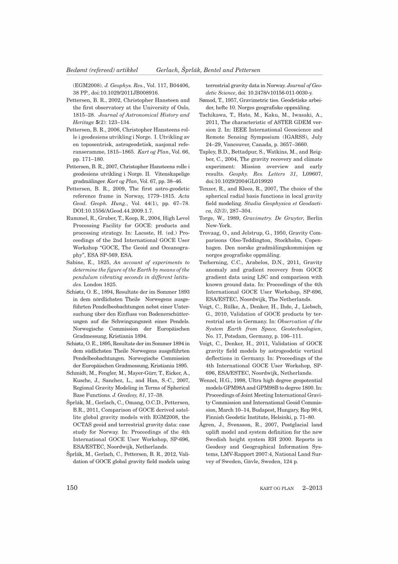
Bedømt (refereed) artikkel Gerlach, Šprlák, Bentel and Pettersen
150 KART OG PLAN 2–2013
(EGM2008). J. Geophys. Res., Vol. 117, B04406,38 PP., doi:10.1029/2011JB008916.
Pettersen, B. R., 2002, Christopher Hansteen andthe first observatory at the University of Oslo,1815–28. Journal of Astronomical History andHeritage 5(2): 123–134.
Pettersen, B. R., 2006, Christopher Hansteens rol-le i geodesiens utvikling i Norge. I. Utvikling aven toposentrisk, astrogeodetisk, nasjonal refe-ranseramme, 1815–1865. Kart og Plan, Vol. 66,pp. 171–180.
Pettersen, B. R., 2007, Christopher Hansteens rolle igeodesiens utvikling i Norge. II. Vitenskapeligegradmålinger. Kart og Plan, Vol. 67, pp. 38–46.
Pettersen, B. R., 2009, The first astro-geodeticreference frame in Norway, 1779–1815. ActaGeod. Geoph. Hung., Vol. 44(1), pp. 67–78.DOI:10.1556/AGeod.44.2009.1.7.
Rummel, R., Gruber, T., Koop, R., 2004, High LevelProcessing Facility for GOCE: products andprocessing strategy. In: Lacoste, H. (ed.) Pro-ceedings of the 2nd International GOCE UserWorkshop “GOCE, The Geoid and Oceanogra-phy”, ESA SP-569, ESA.
Sabine, E., 1825, An account of experiments todetermine the figure of the Earth by means of thependulum vibrating seconds in different latitu-des. London 1825.
Schiøtz, O. E., 1894, Resultate der im Sommer 1893in dem nördlichsten Theile Norwegens ausge-führten Pendelbeobachtungen nebst einer Unter-suchung über den Einfluss von Bodenerschütter-ungen auf die Schwingungszeit eines Pendels.Norwegische Commission der EuropäischenGradmessung, Kristiania 1894.
Schiøtz, O. E., 1895, Resultate der im Sommer 1894 indem südlichsten Theile Norwegens ausgeführtenPendelbeobachtungen. Norwegische Commissionder Europäischen Gradmessung, Kristiania 1895.
Schmidt, M., Fengler, M., Mayer-Gürr, T., Eicker, A.,Kusche, J., Sanchez, L., and Han, S.-C., 2007,Regional Gravity Modeling in Terms of SphericalBase Functions. J. Geodesy, 81, 17–38.
Šprlák, M., Gerlach, C., Omang, O.C.D., Pettersen,B.R., 2011, Comparison of GOCE derived satel-lite global gravity models with EGM2008, theOCTAS geoid and terrestrial gravity data: casestudy for Norway. In: Proceedings of the 4thInternational GOCE User Workshop, SP-696,ESA/ESTEC, Noordwijk, Netherlands.
Šprlák, M., Gerlach, C., Pettersen, B. R., 2012, Vali-dation of GOCE global gravity field models using
terrestrial gravity data in Norway. Journal of Geo-detic Science, doi: 10.2478/v10156-011-0030-y.
Sømod, T., 1957, Gravimetric ties. Geodetiske arbei-der, hefte 10. Norges geografiske oppmåling.
Tachikawa, T., Hato, M., Kaku, M., Iwasaki, A.,2011, The characteristic of ASTER GDEM ver-sion 2. In: IEEE International Geoscience andRemote Sensing Symposium (IGARSS), July24–29, Vancouver, Canada, p. 3657–3660.
Tapley, B.D., Bettadpur, S., Watkins, M., and Reig-ber, C., 2004, The gravity recovery and climateexperiment: Mission overview and earlyresults. Geophy. Res. Letters 31, L09607,doi:10.1029/2004GL019920
Tenzer, R., and Klees, R., 2007, The choice of thespherical radial basis functions in local gravityfield modeling. Studia Geophysica et Geodaeti-ca, 52(3), 287–304.
Torge, W., 1989, Gravimetry. De Gruyter, BerlinNew-York.
Trovaag, O., and Jelstrup, G., 1950, Gravity Com-parisons Olso-Teddington, Stockholm, Copen-hagen. Den norske gradmålingskommisjon ognorges geografiske oppmåling.
Tscherning, C.C., Arabelos, D.N., 2011, Gravityanomaly and gradient recovery from GOCEgradient data using LSC and comparison withknown ground data. In: Proceedings of the 4thInternational GOCE User Workshop, SP-696,ESA/ESTEC, Noordwijk, The Netherlands.
Voigt, C., Rülke, A., Denker, H., Ihde, J., Liebsch,G., 2010, Validation of GOCE products by ter-restrial sets in Germany. In: Observation of theSystem Earth from Space, Geotechnologien,No. 17, Potsdam, Germany, p. 106–111.
Voigt, C., Denker, H., 2011, Validation of GOCEgravity field models by astrogeodetic verticaldeflections in Germany. In: Proceedings of the4th International GOCE User Workshop, SP-696, ESA/ESTEC, Noordwijk, Netherlands.
Wenzel, H.G., 1998, Ultra high degree geopotentialmodels GPM98A and GPM98B to degree 1800. In:Proceedings of Joint Meeting International Gravi-ty Commission and International Geoid Commis-sion, March 10–14, Budapest, Hungary, Rep 98:4,Finnish Geodetic Institute, Helsinki, p. 71–80.
Ågren, J., Svensson, R., 2007, Postglacial landuplift model and system definition for the newSwedish height system RH 2000. Reports inGeodesy and Geographical Information Sys-tems, LMV-Rapport 2007:4, National Land Sur-vey of Sweden, Gävle, Sweden, 124 p.