o l . 8, Is s u E 4, oC T - DE C 2017 ISSN : 2230-7109 (Online ... the name of Incremental Locally linear embedding. Keywords WSN, LLE, ILLE I. Introduction A wireless sensor network

IJECT Vol. 8, IssuE 4, oCT - DEC 2017 ISSN : 2230-7109 (Online) | ISSN : 2230-9543 (Print)

w w w . i j e c t . o r g 46 INterNatIONal JOurNal Of electrONIcS & cOmmuNIcatION techNOlOgy

Localization in Wireless Sensor Network Using Manifold Learning

1Ruchi Tripathi, 2Saurabh Shukla, 3Naresh Patel, 4Shristi Priya1,4Dept. of ECE, Galgotias College of Engineering and Technology, Greater Noida, UP, India

2Goldfame Technologies Private Limited, Gurgaon, Haryana, India3K.D. Polytechnic Patan, Gujarat, India

AbstractThis Paper focuses on Localization in Wireless Sensor Network using a new methodology named Manifold Learning. The localization of wireless sensor network is essential for various applications today which need to know a node’s actual position. Also, there are many factors which affect the performance of any algorithm which has been designed for localization. These factors are discussed in this paper. Localization has become a hot topic of research and many new versions and increments are made to the algorithms for improving the performance. We made use of basically two methods which are applied one after the other. These two techniques come under Manifold learning, the first one is Locally linear embedding; the second is its incremental version by the name of Incremental Locally linear embedding.

KeywordsWSN, LLE, ILLE

I. IntroductionA wireless sensor network is a collection of a very large count of very small wireless sensor nodes which are also termed as the nodes or the sensor nodes which are added very densely to the network. Then the nodes try to discover the conditions which are i.e., they belong to the scenario which is present around. Next the calculations which are made get converted into signals which can be worked upon in order to show certain idea regarding the event. Then we try to route the data which has been gathered to certain unique nodes which are termed as the sink nodes, or the base station; using multi-hop. This can be depicted by the following figure. After that every such node will send the data to users with the use of a satellite or an internet connection via a gateway. However on the basis of what the distance the user is present according to the network; we make use of gateway. This can also be termed as local monitoring.

Fig. 1: A Wireless Sensor Network [14]

With the advancement in technology, it is possible to create an ad-hoc sensor network with the help of cheap nodes which have processors using low power, small amount of memory, a transceiver belonging to wireless network, and a sensor board. A common node is similar to 2AA batteries in size. There are

much new application coming up, for example, habitat monitoring, tracking the target, detecting and reporting failure in building. For such applications it becomes important to strictly orient all the nodes depending on a global coordinate system, so that we can make a report for data which has some geographical meaning. Also the general middle ware services for example routing are based on the location information. This is also called as geographical routing. Hence localization of sensor nodes with good accuracy is very important for various applications.

II. MotivationThe Motivation of this thesis comes from the application of local linear embedding in order to find out sensor node embeddings on the basis of their adjacent nodes. We chose the neighbors on the basis of some factors like the hop count, meaning that the sensor which islocated at a distance of single hop count with respect to a particular sensor node can be termed as the neighbors. When we know who the neighbors are, plus there locations, then we can compute the local embeddings, with the help of LLE and ILLE for the wireless sensor network. It can be presumed that we have an availability of sufficient number of anchor node which is deployed in the sensor network, and their global coordinates can be accurately assessed using GPS or similar technology. With the help of this information, also the local embedding; the global coordinates of a node can be accurately foundout.

A. Currently Existing TechnologiesThere are many techniques developed for localization in WSN. Some of the important researches done are as follows.

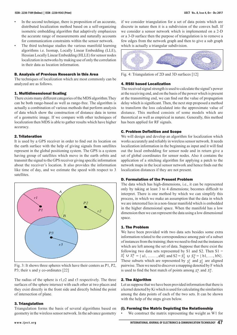
The first technique makes use of the geodesic distances in place • of Euclidean distances in order to calculate the differences among the sensors, and then use the isomap algorithm (a technique of manifold learning) in order to compute the relative locations of sensors. The isomap algorithm is a manifold learning technique, which was actually aimed for decreasing the non-linear dimension, and then we use it broadly for finding the differences among the data set. It can also be used for determining the spatial construction in data having low- dimensions.

Fig. 2: Depicts the Non-Linear Reduction of Dimensions Elaborately [2]

IJECT Vol. 8, IssuE 4, oCT - DEC 2017

w w w . i j e c t . o r g INterNatIONal JOurNal Of electrONIcS & cOmmuNIcatION techNOlOgy 47

ISSN : 2230-7109 (Online) | ISSN : 2230-9543 (Print)

In the second technique, there is proposition of an accurate, • distributed localization method based on a self-organizing isometric embedding algorithm that adaptively emphasizes the accurate range of measurements and naturally accounts for communication constraints within the sensor network.The third technique studies the various manifold learning • algorithms i.e. Isomap, Locally Linear Embedding (LLE), Hessian Locally Linear Embedding (HLLE) for sensor nodes localization in networks by making use of only the correlation in their data as location information.

B. Analysis of Previous Research in this AreaThe techniques of localization which are most commonly can be analyzed are as follows.

1. Multidimensional ScalingThere exists many different categories of the MDS algorithm.They can be both range-based as well as range-free. The algorithm is actually a combination of various methods that perform analysis of data which show the construction of distance data in terms of a geometric image. If we compare with other techniques of localization then MDS is able to gather results which have higher accuracy.

2. TrilaterationIt is used by a GPS receiver in order to find out its location on the earth surface with the help of giving signals from satellites represent in the global positioning system. The GPS is a system having group of satellites which move in the earth orbits and transmit the signal to the GPS receiver giving specific information about the receiver’s location. It also provides the information like time of day, and we estimate the speed with respect to 3 satellites.

Fig. 3: It shows three spheres which have their centers as P1, P2, P3; their x and y co-ordinates [22]

The radius of the sphere is r1,r2 and r3 respectively. The three surfaces of the sphere intersect with each other at two places and they exist directly in the front side and directly behind the point of intersection of plane.

3. TriangulationTriangulation forms the basis of several algorithms based on geometry in the wireless sensor network. In the advance geometry

if we consider triangulation for a set of data points which are discrete in nature then it is a subdivision of the convex hull. If we consider a sensor network which is implemented on a 2-D or a 3-D surface then the purpose of triangulation is to remove a few edges from the network graph and then to give a sub graph which is actually a triangular subdivision.

Fig. 4: Triangulation of 2D and 3D surfaces [12]

4. RSSI based LocalizationThe received signal strength is used to calculate the signal’s power at the receiving end, and on the basis of the power which is present at the transmitting end, we can find out the value of propagation delay which is significant. Then, the next step proposed a method to transform the loss calculated into the approximate value of distance. This method consists of some models which are theoretical as well as empirical in nature. Generally, this method has been applied for RF signals.

C. Problem Definition and Scope We will design and develop an algorithm for localization which works accurately and reliably in wireless sensor network. It needs localization information in the beginning as input and it will find out the local embedding for sensor node and in return give a set of global coordinates for sensor nodes. Also it contains the application of a stitching algorithm for applying a patch to the network maps in the local sensor network and hence finds out the localization distances if they are not present.

D. Formulation of the Present ProblemThe data which has high-dimensions, i.e., it can be represented only by taking at least 3 to 4 dimensions; becomes difficult to interpret. There is one method by which we can simplify this process, in which we make an assumption that the data in which we are interested lies in a non-linear manifold which is embedded in the higher dimensional space. When the manifold has a low dimension then we can represent the data using a low dimensional space.

1. The ProblemWe have been provided with two data sets besides some extra information related to the correspondence among pair of a subset of instances from the training; then we need to find out the instances which are left among the set of data. Suppose that there exist the following two data sets represented by S1 and S2. Then S1 =

= { a1, …… , aM} and S2 = = { b1, …., bN}. These subsets which are represented by and are aligned pairwise. Then we need to discover a mapping denoted by F which is used to find the best match of points among and .

2. The AlgorithmLet us suppose that we have been provided information that there is a kernel denoted by Ki which is used for calculating the similarities among the data points of each of the two sets. It can be shown with the help of the steps given below.

(i). Forming the Matrix Depicting the RelationshipWe construct the matrix representing the weight as W1 for •



the set S1 and then W2 for the set S2 with the help of Kp, when we have that W1 ( p,q) = K1( ap, aq) and W2 (p,q) = K2( bp, bq).Then find out the Laplacian matrix L1 and L2, where L1 and • L2 are computed using the identity matrix I and the diagonal matrix DK.

(ii). Learning the Embedding of Low Dimensions Belonging to the Data SetWe find out the values of the chosen Eigenvectors belonging to the matrix L1 and L2. They are determined as the embedding of low dimensions belonging to the data set S1 and S2. Suppose that A, Au represent the d-dimensional embeddings for the subsets and ; then B, Bu represents the d-dimensional embeddings for the subsets and . Here we have that the subsets occur in a pairwise alignment with each other as follows .

(iii). Determining the Optimal Alignment for A and B.In this step we perform translation for the configurations in • A, Au, B, Bu; in order to let A and B get their centroids at the starting point.Next we find out the SVD which denotes the singular value • decomposition for BTA.Then we compute B* which is = kBR. It denotes the optimal • results of mapping which are used to minimize || A- B*||. The double mod notation shows the Frobenius Norm. Also R = UVT whereas, k = trace () / trace (BTB).

(iv). Next we employ R and k to determine the correspondences among .Bu* = k BuR.For every element ‘a’ which belongs to Au, then its correspondences in Bu* = argminb* ∈Bu* || b* - a||.

Fig. 5: Depicts the Different Alignments. [17]

It depicts the comparison between manifolds a1 which is red, • a2 which is blue and a3 which is green before the process of alignment. This figure shows 3D alignment by the technique of multiple • manifold alignment. It shows 2D alignment using the technique of multiple • manifold alignment. This figure depicts the 1D alignment with the use of multiple • manifold alignment.

III. Theoretical Tools- Analysis and DevelopmentIf we consider mathematically, then the manifold of dimensions N is topologically available in space, which has a similarity with the Euclidean space in the N- dimension. To state in an exact manner, then every point in the N- dimension space of manifold gets a locality which is homeomorphism with respect to N dimensions in the Euclidean space. Example of such 1D manifold is lines and circles. The surfaces are 2D manifold. 3D manifolds are plane, torus, and sphere.

A. Isomap AlgorithmThe main goal of this algorithm is to select a presentation of data in very low-dimensions. It maintains the optimal value for the distance among any two input points, according to the measurement of the geodesic distance with the manifold. It finds out the estimate of geodesic distance in terms of a series of skips among the adjacent data points. The value becomes accurate from being simple approximate, inside the infinite data limit. A version of classical MDS is the Isomap algorithm, which uses the geodesic distance instead of the Euclidean distance.

Fig. 6: It shows the Various Manifold Learning Techniques Having 1000 Data Points and 10 Neighbors.

For computing the Isomap algorithm needs three steps which can be stated as follows:(1) In the input space, determine the adjacent points which are closest upto T number of times for every data point; then form a graph which is undirected and represented by G, in which the data points will be represented as the nodes of the graph and the link among the adjacent points can be represented as the edges. The time complexity for this step is O (N2).(2) Then calculate an estimate of the geodesic distance which is represented by the symbol (a, b); and is present for any two nodes say (a, b) by determining the shortest path in the graph G with the usage of Dijkstra’s algorithm which is applied to every node of the graph. Next we form a matrix of N X N which is dense in nature; it is a similarity matrix, denoted by says, G, through the centering ∆2 (a, b) in which the main aim is to create a similarities from the distances. The time complexity for this step is O (N2 log N). It depends mainly on the computations involves in geodesic distance.(3) Next we try to determine the optimal value of K, as the dimensional representation, X= {xa}

N for value of a=1, in a manner

that X = argminX’ . Then finally after solving we get the following:

.




Here the summation ΣK represents the matrix K X K which stores the upper K eigenvalues of the graph G, whereas, ∪K represents the eigenvectors which are related to each other. The space complexity of this step is O (N2) and the time complexity is O (N3) for the purpose of decomposing the Eigen values.

When the value of N becomes equal to 18 M, then it is not possible to trace the time complexity and the space complexity.

B. Locally Linear Embedding:This algorithm is formed by simple geometrical analysis. Let us consider that we have N vectors having real values, their dimension is represented by d if the needed data is present then we can have an idea about each data point and its adjacent points, that they are on top of or very near to local linear patch. We can implement the algorithm in a straight way, because it has just one parameter which is free. This parameter is denoted by K and it represents the count of adjacent points for each data points. As soon as we select the neighbors, the weight Wij and coordinates Yi are calculated by regular methods of linear algebra. This can be shown by the following figure which depicts the three steps of the algorithm.

LLE algorithmStep 1: We find out the adjacent point for each data point Xi.Step 2: Find out the weights Wij which perform the optimum reconstruction of every data point Xi from its adjacent points, which minimizes the cost equation 1.Step 3: Find out the vector Yi which is optimally reconstructed by the weights Wij, this minimizes the quadratic in equation 2 from the bottom Eigen vectors that are non-zero values.

Fig. 7: This is an example of Swiss Roll. The figures B and C have a black box, which show the way in which a locally linear plot of points is protruded down into 2 dimensions. [2]

Fig. 8: This figure shows an open ball. Initially the points are distributed along the open ball in 3D space; it is then projected down into 2D space. [22]

C. Incremental Locally Linear Embedding:This algorithm is the incremental version of the LLE algorithm. This algorithm is suitable for application in real time. In which we require a constant data measurement. It provides the same accuracy as the LLE algorithm. However there is an important increase in speed when the data has to be added constantly.

LLE belongs to the family of unsupervised techniques of manifold learning. Such algorithms demand very high computational power. One important set back in this technique, is their operation in batch mode, meaning that a large block of data gets processed at the same time. Also it is not able to re-use the information coming from the previous run, and requires restarting the entire calculation from the beginning even when you get a very small change in the set of data points. This creates big problems when you are operating an online analysis of data which is also time critical in nature. In this situation there is a huge consumption of CPU power, memory, etc.

Along with the above discussed problem, in batch mode processing there is a substantial amount of delay introduced. This proves to be damaging for some application in which the system has to give a reaction for an input. Hence we required to formulate an incremental approach so that the LLE become suitable in real time application.

This will speed up the calculation when we are modifying an a data set which already exist. When we add one data sample to the set, and extend the embedding, then the incremental LLE algorithm will make an attempt to reuse the information and other results that have been collected during the previous embedding. The following table represent the run time which is required by the different components of the algorithm.

Table 1: The Percentage of Run Time Taken by Different Parts of the Algorithm [1]

Step Action performed % of run Time

1 Compute distances between samples 9.9

1 Find nearest neighbors 28.4

2 Compute restoration weights 4.6

2 Save restoration weights 20.9

3 Perform embedding 25.2

Other tasks 11.0

D. Testing and Analysis We begin by taking a set of data that has 500 samples in the swissroll and then finding out the embeddings. After that a comparison is made between LLE and ILLE with the addition of new samples to the data set and then again computing the matching embedding. Then we find out the number of iterations which are needed for the algorithm which has been laid for proposition by the use of some power iterations; this is required to update the embeddings. The figure below shows the count of iteration, for both computations which involve EVD with LLE and EVD with ILLE.



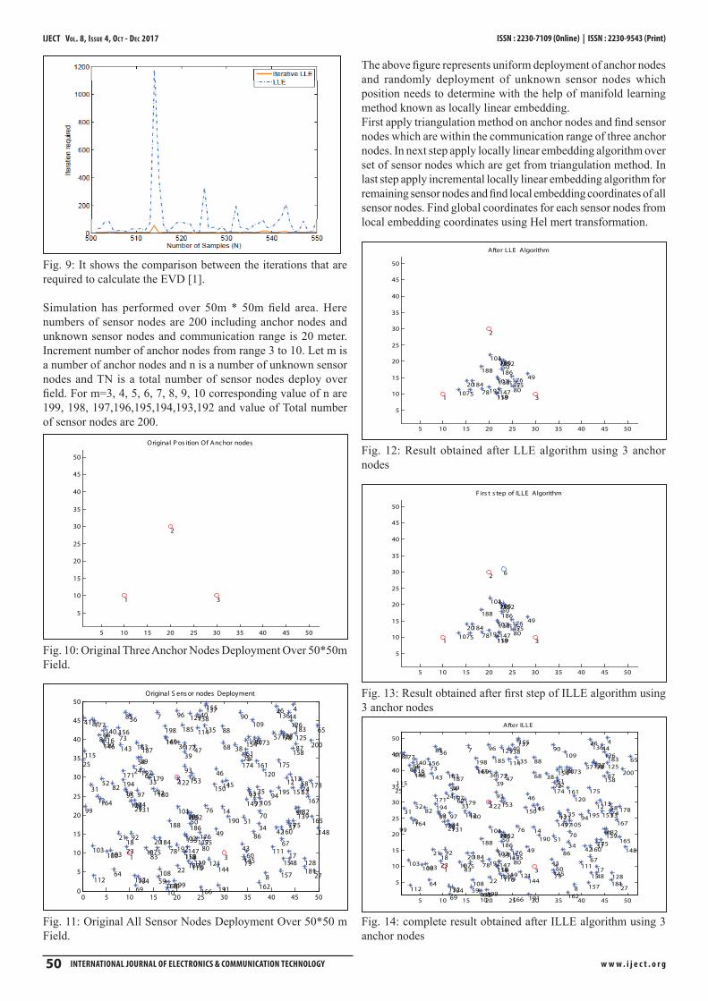
Fig. 9: It shows the comparison between the iterations that are required to calculate the EVD [1].

Simulation has performed over 50m * 50m field area. Here numbers of sensor nodes are 200 including anchor nodes and unknown sensor nodes and communication range is 20 meter. Increment number of anchor nodes from range 3 to 10. Let m is a number of anchor nodes and n is a number of unknown sensor nodes and TN is a total number of sensor nodes deploy over field. For m=3, 4, 5, 6, 7, 8, 9, 10 corresponding value of n are 199, 198, 197,196,195,194,193,192 and value of Total number of sensor nodes are 200.

5 10 15 20 25 30 35 40 45 50

5

10

15

20

25

30

35

40

45

50

Original P os ition Of Anchor nodes

1

2

3

Fig. 10: Original Three Anchor Nodes Deployment Over 50*50m Field.

0 5 10 15 20 25 30 35 40 45 500

5

10

15

20

25

30

35

40

45

50Original S ens or nodes Deployment

1

2

3

4

5

6

7

89

10

11 12

1314

15

16

17

18

19

2021

22

23

2425

26

27

2829

30

31

32

33

34

35

36

37

3839

4041

42

43

44

45

46

47

48

49

50 51

5253

54

55

56

57

58

59

60

61

62

63

64

6566

67

68

69

7071

72

73

74

75

7677

78

79

80

81

82

83

84

85

86

87

88

89

90

91

92

93

9495

96

97

98

99

100

101

102

103

104

105

106

107

108

109

110

111

112

113

114

115

116

117

118119

120

121

122

123124

125

126

127

128

129

130

131

132

133

134

135

136137

138

139

140141

142

143

144145

146

147

148

149

150 151

152

153

154

155

156

157

158

159

160

161

162

163

164

165

166

167

168

169170

171

172173

174 175

176

177

178179

180

181

182

183

184

185

186

187

188

189

190

191

192193

194195

196

197

198

199

200

Fig. 11: Original All Sensor Nodes Deployment Over 50*50 m Field.

The above figure represents uniform deployment of anchor nodes and randomly deployment of unknown sensor nodes which position needs to determine with the help of manifold learning method known as locally linear embedding.First apply triangulation method on anchor nodes and find sensor nodes which are within the communication range of three anchor nodes. In next step apply locally linear embedding algorithm over set of sensor nodes which are get from triangulation method. In last step apply incremental locally linear embedding algorithm for remaining sensor nodes and find local embedding coordinates of all sensor nodes. Find global coordinates for each sensor nodes from local embedding coordinates using Hel mert transformation.

5 10 15 20 25 30 35 40 45 50

5

10

15

20

25

30

35

40

45

50

After LLE Algorithm

1

2

35

20

28

49

50

5578 80

101

102

106

107117

118

133

147

152

159

176184

186188

192

Fig. 12: Result obtained after LLE algorithm using 3 anchor nodes

5 10 15 20 25 30 35 40 45 50

5

10

15

20

25

30

35

40

45

50

F irs t s tep of ILLE Algorithm

1

2

35

20

28

49

50

5578 80

101

102

106

107117

118

133

147

152

159

176184

186188

192

6

Fig. 13: Result obtained after first step of ILLE algorithm using 3 anchor nodes

5 10 15 20 25 30 35 40 45 50

5

10

15

20

25

30

35

40

45

50

After ILLE

1

2

35

20

28

49

50

5578 80

101

102

106

107117

118

133

147

152

159

176184

186188

192

6

9

10

11

14

18

19

21

22

23

24

29

33

34

35

3639

42

43

45

46

47

51

52

54

59

60

61

62

63

64

67

68

69

7071

72

73

74

75

7677

79

82

83

84

86

88

89

91

92

93

9495

96

97

98

99

100103

104

105

108

109

110

111

112

113

114

115

116

119

120

121

122

123124

125

126

127

128

129

130

131

132

134

135

136137138

139

140141

142

143

144145

146

148

149

150151

153

154

155

156

157

158

160

161

162

163

164

165

166

167

168

169170

171

172173

174 175

177

178179

180

181

182

183185

187

189

190

191

193

194195

196

197

198

199

200

47

8

12

13

15

16

17

25

26

27

30

31

32

37

38

4041

44

48

53

56

57

58

6566

8185

87

90

Fig. 14: complete result obtained after ILLE algorithm using 3 anchor nodes




Now I will explain another simulation that performed over 50m * 50m field area. Here numbers of sensor nodes are 200 including anchor nodes and unknown sensor nodes and communication range is 20 meter.

5 10 15 20 25 30 35 40 45 50

5

10

15

20

25

30

35

40

45

50

After ILLE

1

2

3

4

5

6

78

9 10

11

12

14

1518

1920

22

23

25

26

27

28

2930

31

32

33

36

37

3839

40

43

454647

49

50

51

52

53

5657

60

61

62

63

65

66

67

68

70

73

74

76

7778

79

81

82

83

84

85

86

87

88

90

91

92 93

94

96

97

9899

100101

103

104

106

107

108

109

111

114

115

116

120

121

122

125

126

127

129131

132

134

135

138

139

141

142

146

148

149

150

153

154

155

156

158

159

160

161162

163

164

165

166

168169

170

172

173

176

177

178

179

180

186

187

188 189

190

191192

193

195 196

197

198

199

1316

17

21

2434 35

41

42

44

48

54 55

5859

64

6971 72

7580

89

95

102

105110

112

113117

118

119

123

124128

130

133

136 137

140

143

144

145

147

151

152

157

167

171

174

175

181

182

183

184

185

194

200

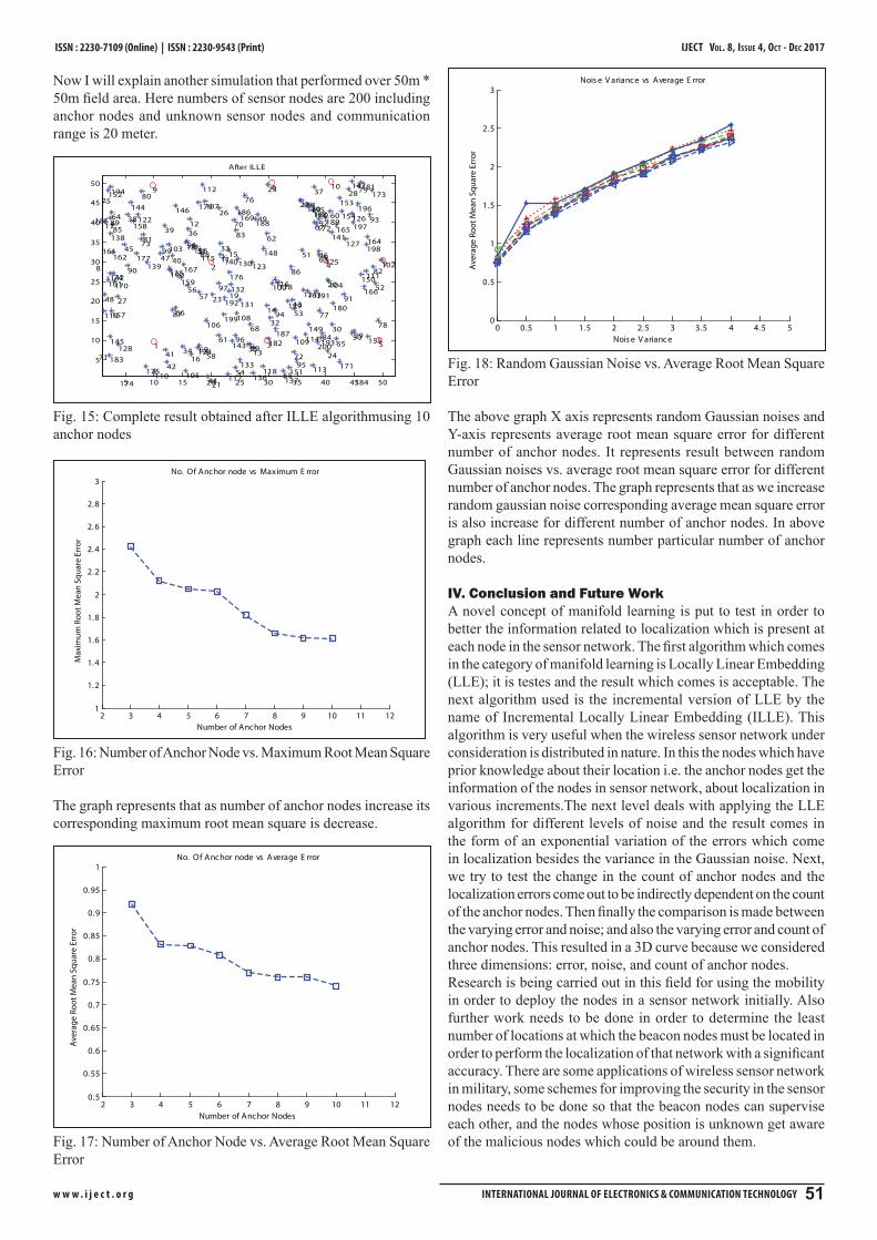
Fig. 15: Complete result obtained after ILLE algorithmusing 10 anchor nodes

2 3 4 5 6 7 8 9 10 11 121

1.2

1.4

1.6

1.8

2

2.2

2.4

2.6

2.8

3

Number of Anchor Nodes

Max

imum

Roo

t Mea

n Sq

uare

Err

or

No. Of Anchor node vs Maximum E rror

Fig. 16: Number of Anchor Node vs. Maximum Root Mean Square Error

The graph represents that as number of anchor nodes increase its corresponding maximum root mean square is decrease.

2 3 4 5 6 7 8 9 10 11 120.5

0.55

0.6

0.65

0.7

0.75

0.8

0.85

0.9

0.95

1

Number of Anchor Nodes

Ave

rage

Roo

t Mea

n Sq

uare

Err

or

No. Of Anchor node vs Average E rror

Fig. 17: Number of Anchor Node vs. Average Root Mean Square Error

0 0.5 1 1.5 2 2.5 3 3.5 4 4.5 50

0.5

1

1.5

2

2.5

3

Nois e V ariance

Ave

rage

Roo

t Mea

n Sq

uare

Err

or

Nois e V ariance vs Average E rror

Fig. 18: Random Gaussian Noise vs. Average Root Mean Square Error

The above graph X axis represents random Gaussian noises and Y-axis represents average root mean square error for different number of anchor nodes. It represents result between random Gaussian noises vs. average root mean square error for different number of anchor nodes. The graph represents that as we increase random gaussian noise corresponding average mean square error is also increase for different number of anchor nodes. In above graph each line represents number particular number of anchor nodes.

IV. Conclusion and Future WorkA novel concept of manifold learning is put to test in order to better the information related to localization which is present at each node in the sensor network. The first algorithm which comes in the category of manifold learning is Locally Linear Embedding (LLE); it is testes and the result which comes is acceptable. The next algorithm used is the incremental version of LLE by the name of Incremental Locally Linear Embedding (ILLE). This algorithm is very useful when the wireless sensor network under consideration is distributed in nature. In this the nodes which have prior knowledge about their location i.e. the anchor nodes get the information of the nodes in sensor network, about localization in various increments.The next level deals with applying the LLE algorithm for different levels of noise and the result comes in the form of an exponential variation of the errors which come in localization besides the variance in the Gaussian noise. Next, we try to test the change in the count of anchor nodes and the localization errors come out to be indirectly dependent on the count of the anchor nodes. Then finally the comparison is made between the varying error and noise; and also the varying error and count of anchor nodes. This resulted in a 3D curve because we considered three dimensions: error, noise, and count of anchor nodes.Research is being carried out in this field for using the mobility in order to deploy the nodes in a sensor network initially. Also further work needs to be done in order to determine the least number of locations at which the beacon nodes must be located in order to perform the localization of that network with a significant accuracy. There are some applications of wireless sensor network in military, some schemes for improving the security in the sensor nodes needs to be done so that the beacon nodes can supervise each other, and the nodes whose position is unknown get aware of the malicious nodes which could be around them.



References[1] Sebastian Schuon, Marko Durkovic, Klaus Diepold,

JurgenScheuerle, Stefan Markward,“Truly Incremental Locally Linear Embedding”, In Proceedings of the CoTeSys 1st International Workshop on Cognition for Technical Systems, October 2008.

[2] Lawrence K. Saul, Sam T. Roweis,“An Introduction to Locally Linear Embedding”, in 2000.

[3] MarziaPolito, PietroPerona,“Grouping and Dimensionality Reduction by Locally Linear Embedding”, NIPS, 2001.

[4] Chengqun Wang, Jiming Chen, Youxian Sun, Xuemin (Sherman) Shen,“Wireless Sensor Networks Localization with Isomap”, Communications ICC ‘09 IEEE International Conference, 14-18 June 2009.

[5] Shancang LI, Deyun ZHANG,“A Novel Manifold Learning Algorithm for Localization Estimation in Wireless Sensor Networks”, IEICE Trans. Commun., Vol. E90–B, No.12, 2007.

[6] Neal Patwari, Alfred O. Hero III, “Manifold Learning Algorithms for Localization in Wireless Sensor Network”, Acoustics, Speech, and Signal Processing Proceedings. (ICASSP ‘04). IEEE International Conference, 2004.

[7] Olga Kouropteva, Oleg Okun, MattiPietikainen, “Incremental Locally Linear Embedding Algorithm”, H. Kalviainen et al. (Eds.): SCIA 2005, LNCS 3540, pp. 521–530, 2005. Springer-Verlag Berlin Heidelberg, 2005.

[8] MasoomehRudafshani, SuprakashDatta, “Localization in Wireless Sensor Networks”, IPSN’07, Cambridge, Massachusetts, USA. Copyright ACM 978-1-59593-638-7/07/0004, 2007.

[9] RashmiAgrawal, Brajesh Patel, “Localization in Wireless Sensor Network Using MDS”, International Journal of Smart Sensors and Ad Hoc Networks (IJSSAN) ISSN No. 2248-9738, Vol. 1, Issue 3, 2012.

[10] ShailajaPatil, MukeshZaveri, “MDS and Trilateration Based Localization in Wireless Sensor Network”, Vol. 3 No. 6, pp. 198-208. doi: 10.4236/wsn.2011.36023, 2011.

[11] Yi Shang, Wheeler Ruml,“Improved MDS-Based Localization”, INFOCOM 2004. Twenty-third Annual Joint Conference of the IEEE Computer and Communications Societies (Vol. 4), 2004.

[12] Hongyu Zhou, Hongyi Wu, Su Xia, Miao Jin, Ning Ding, “A Distributed Triangulation Algorithm for Wireless Sensor Networks on 2D and 3D Surface”, INFOCOM, 2011 Proceedings IEEE, April 2011.

[13] A. R. Kulaib, R. M. Shubair, M. A. Al-Qutayri, Jason W. P. Ng, “An Overview of Localization Techniques for Wireless Sensor Networks”, Innovations in Information Technology (IIT), 2011 International Conference on, April 2011.

[14] Lina M. PestanaLeão de Brito, Laura M. Rodríguez Peralta, “An Analysis of Localization Problems and Solutions in Wireless Sensor Networks”, Polytechnical Studies Review, Vol VI, ISSN: 1645-9911, 2008.

[15] Gowrishankar.S, T.G.Basavaraju, Manjaiah D.H, Subir Kumar Sarkar,“Issues in Wireless Sensor Networks”, Proceedings of the World Congress on Engineering 2008 Vol. 1, WCE 2008, London, U.K., July, 2008.

[16] Sam Roweis, Lawrence K. Saul, Geoffrey E. Hinton, “Global Coordination of Local Linear Models”, Neural Information Processing Systems 14 (NIPS’01). pp. 889-896, 2002.

[17] Chang Wang, Sridhar Mahadevan,“Manifold Alignment using Procrustes Analysis”, Proceedings of the 25th

International Conference on Machine Learning, Helsinki, Finland, 2008.

[18] Amitangshu Pal, “Localization Algorithms in Wireless Sensor Networks: Current Approaches and Future Challenges”, Network Protocols and Algorithms ISSN 1943-3581, Vol. 2, No. 1, In 2010.

[19] Martin H.C. Law, Anil K. Jain, “Incremental Nonlinear Dimensionality Reduction by Manifold Learning”, IEEE Transactions on Pattern Analysis and Machine Intelligence, Vol. 28, No. 3, March 2006.

[20] Matthew Brand, “Charting a manifold”, TR-2003-13, 2003.

[21] J. Carey, G. Quinn, M. Burgman, “Multidimensional Scaling”, BIOL90002 Biometry, 2011.

[22] Lawrence K. Saul, SamT. Roweis,“Think Globally, Fit Locally: Unsupervised Learning of Low Dimensional Manifolds”, Journal of Machine Learning Research 4 (2003) 119-155, 2003.

Ruchi Tripathi has received her B.E. Degree in Electronics Engineering from M.I.T.S Gwalior in 2009, M.Tech Degree in Communication Engineering from IIIT Allahabad in 2014. She was lecturer in ACTS Satna (M.P.) from July 2009 to June 2011. She has worked as Assistant Professor in PSIT Kanpur (U.P) from June 2014 to April 2017, ECE Department. Presently, she is working as Assistant Professor

in GCET greater Noida, ECE Department. Her area of interest is Wireless Communication and Networking, Wireless Sensor Networks and Network Coding.

Saurabh Shukla has received his B.E. Degree in Electronics and Communication Engineering from RGPV Bhopal in 2014, Pursuing M.Tech from Amity University Gurgaon (weekend classes). He has worked as Electronics Engineer in SMT Gurgaon and Presently working in Goldfame Technologies Private Limited as Quality Head from October 2016. His area of Interest is

Electronics Devices and Components.

Documents

o l . 8, Is s u E 4, oC T - DE C 2017 ISSN : 2230-7109 (Online ... the name of Incremental Locally linear embedding. Keywords WSN, LLE, ILLE I. Introduction A wireless sensor network