Embed Size (px)
Citation preview

Numerics for Partial Differential Equations
a.o.Univ.Prof. Mag.Dr. Stephen Keelinghttp://imsc.uni-graz.at/keeling/
Documentation und Literature:http://imsc.uni-graz.at/keeling/teaching.html
These notes are based especially upon works of:Vasilios Dougalis, Randall LeVeque and Christian Clason
but also upon works of:Franz Kappel, Kazufumi Ito, Karl Kunisch and David Gottlieb
1

Table of Contents IIntroduction
Types of PDEsElliptic PDEsParabolic PDEsHyperbolic PDEsConvection Diffusion EquationHyperbolic SystemsClassical Solution ProceduresWell-Posed BVPs
Finite Difference Methods for Elliptic ProblemsDirichlet Problem for the Poisson EquationDiscrete LaplacianShortley-Weller FormulaFinite Difference SchemeDiscrete Maximum and Minimum PrinciplesExistence of a SolutionDiscrete Green’s FunctionProperties of the Discrete Green’s FunctionConvergence of the Discrete SolutionNeumann Problem for the Poisson EquationFinite Difference SchemeMonotone MatricesExistence of a Discrete SolutionConvergence of the Discrete SolutionElliptic BVPs with Variable CoefficientsFinite Difference SchemeNon-Linear Elliptic BVPDirichlet Poisson BVP on a SquareNeumann Poisson BVP on a SquareNon-Linear Elliptic BVP on a Square
Finite Difference Methods for Parabolic ProblemsHeat EquationExplicit Finite Difference Scheme2

Table of Contents IIStability of Explicit SchemeConsistency of Explicit SchemeConvergence of Explicit SchemeNeumann Heat Equation on a SquareSemi-Discrete SolutionExplicit and Implicit Euler SchemesNon-Linear Parabolic IBVPCode to Solve the Non-Linear IBVP
Finite Difference Methods for Hyperbolic ProblemsWave EquationExplicit Finite Difference SchemeInitial Conditions of Explicit SchemeConsistency of Explicit SchemeForward, Backward, Centered DifferencesBilinear FormConvergence of Explicit SchemeDirichlet Wave Equation on a SquareProperties of First Order FormSemi-Discrete SolutionCrank Nicholson SchemeNon-Linear Hyperbolic IBVP for a CordCode to Solve the Non-Linear IBVP
Finite Difference Methods for Conservation LawsScalar Convection EquationFinite Difference SchemeFourier TransformsConsistency of the Forward Difference SchemeStability of the Forward Difference SchemeSobolev SpacesConvergence of the Forward Difference SchemeBackward Difference SchemeLax Wendroff SchemeLinear Hyperbolic Systems3

Table of Contents IIIInflow Boundary ConditionsUpwinding and Other Single-Step SchemesConsistency of Single-Step SchemesStability of Single-Step SchemesLax Equivalence TheoremComputing Discontinuous SolutionsModified EquationsDissipation and DispersionPhase and Group VelocitiesRelative Dissipation and Dispersion ErrorsBurger’s EquationConservative Methods for Nonlinear ConvectionConsistency for Conservative MethodsLax Wendroff TheoremVanishing Viscosity and Entropy SolutionsRoe’s Approximate Riemann SolverCode to Solve Burger’s EquationRoe Matrix for Isothermal FlowConvection Diffusion EquationCode to Solve Convection Diffusion PDE
Variational Theory of PDEsFunction Spaces for Elliptic PDEsLebesgue and Holder SpacesWeak Derivatives and Sobolev SpacesSobolev EmbeddingsTracesPoincare’s InequalityWeak Formulation of Elliptic BVPsLax Milgram TheoremRegularity of Weak Solutions to Elliptic BVPsFunction Spaces for Evolution EquationsWeak Formulation of Parabolic IBVPsLumer Philips Theorem4

Table of Contents IVExistence of Semigroups and Weak SolutionsWeak Formulation, Non-Autonomous Parabolic PDEs
Finite Element Methods for Elliptic ProblemsConforming Finite Element MethodsCea’s LemmaRitz-Galerkin ApproximationAubin Nitsche LemmaFEM for Dirichlet Poisson BVP on a SquareError Estimate for Dirichlet Poisson BVPError Estimate for Interpolation OperatorsEnergy Estimate for Dirichlet Poisson BVPL2 Estimate for Dirichlet Poisson BVPImplementation of FEM Solver on a SquareElement Based AssemblyForm FunctionsExplicit Calculation of Stiffness MatrixExplicit Calculation of Mass MatrixCode for Dirichlet Poisson BVP on a squareA Posteriori Error Estimates and AdaptivityFinite Element SpacesExamples of Finite ElementsTriangular ElementsRectangular ElementsThe InterpolantTriangulationsContinuity of Finite Element SpaceAffine Equivalent Finite ElementsPolynomial Interpolation in Sobolev SpacesBramble Hilbert LemmaInterpolation Error EstimatesLocal Interpolation ErrorGlobal Interpolation Error5

Table of Contents VInverse Error EstimatesError Estimates for Finite Element ApproximationsA Posteriori Error EstimatesDuality Based A Posteriori Error EstimatesImplementationAssemblyQuadratureGeneralized Galerkin ApproachBanach Necas Babuska TheoremFirst Strang LemmaSecond Strang LemmaEstimation of Quadrature ErrorsDiscontinuous Galerkin ApproachMixed Finite Element MethodsMixed FEM for Piecewise Constant Data
Finite Element Methods for Evolution EquationsTrotter Kato TheoremStability, Consistency, StabilityAlternative Consistency ConditionApplication to the Convection EquationApplication to the Heat EquationApplication to the Wave EquationSpectral Methods for Evolution EquationsNon-Autonomous Evolution EquationsSpace-Time Galerkin Schemes
6

Types of PDEsI The standard types of partial differential equations (PDEs)
are: elliptic, parabolic and hyperbolic.I There are standard algebraic defintions of these types
which one encounters in the continuum study of PDEs.I For instance, the PDE
auxx (x , y)+buxy (x , y)+cuyy (x , y)+dux (x , y)+euy (x , y) = 0
I is elliptic if b2 − ac < 0,I parabolic if b2 − ac = 0, andI hyperbolic if b2 − ac > 0.
I But what about more complex PDEs? Equation type istypically defined in terms of characteristics, which may bedefined for systems as well as for nonlinear problems.
I Especially for the numerical solution of PDEs we mayunderstand these types qualitatively and intuitively in termsof the standard model equations.
7

Elliptic PDEsI Elliptic PDEs are found typically in the modelling of
stationary fields such as force-at-a-distance fields.I For such PDEs every point is coupled with every other
point, and there is no notion of evolution in time.I Consider the displacement field of an unloaded membrane
with a curved fixed boundary, modelled by the followingLaplace Equation with a boundary condition.
uxx (x , y) + uyy (x , y) = 0, for (x , y) ∈ Ω = B(0,1)u(x , y) = g(x , y), for (x , y) ∈ ∂Ω
Withg(x , y) = sin(3 tan−1(y/x))
the solution is
u(x , y) = (x2 + y2)32 sin(3 tan−1(y/x))
8

Parabolic PDEsI Parabolic PDEs are found typically in the modelling of
diffusion processes.I For such PDEs every point in space is coupled with every
point in space, and there is an evolution in time which issmoothing since information travels at an infinite speed.
I Consider the evolution of temperature between suddenlyconnected hot and cold regions, modelled by the followingHeat Equation with an initial condition.
ut (x , t) = uxx (x , t), for (x , t) ∈ R× (0,∞)u(x ,0) = u0(x), for (x , t) ∈ R× 0
Withu0(x) = 1
2 [1 + sign(x)]
the solution is
u(x , t) = 12 [1 + erf(x/
√4t)]
9

Hyperbolic PDEsI Hyperbolic PDEs are found typically in the modelling of
waves.I For such PDEs there is an evolution in time which is not
smoothing since information travels at a finite speed.I Consider the evolution of displacement in a string suddenly
stretched in a finite region, modelled by the following WaveEquation with initial conditions.
utt (x , t) = uxx (x , t), for (x , t) ∈ R× (0,∞)u(x ,0) = u0(x), for (x , t) ∈ R× 0ut (x ,0) = u1(x), for (x , t) ∈ R× 0
With u1(x) = 0 and
u0(x) = sign(x + 1)− sign(x − 1)
the solution is
u(x , t) = 12 [sign(x +t +1)−sign(x +t−1)]
+12 [sign(x−t +1)−sign(x−t−1)]
10

Convection Diffusion EquationI But what about the following convection (velocity ν > 0)
and diffusion (diffusivity ε > 0) equation?ut (x , t) + νux (x , t) = εuxx (x , t), for (x , t) ∈ R× (0,∞)
u(x ,0) = g(x), (x , t) ∈ R× 0
Withg(x) = sign(x + 1)− sign(x − 1)
the solution is
u(x , t) =12
erf[νt − x + 1√
4εt
]− 1
2erf[νt − x − 1√
4εt
]
I This solution manifests more wave character when ν εand more diffusion character when ε ν.
I The situation is more complex for non-linear PDEs, but wewill use the linear problems presented here as model problemsupon which methods for non-linear problems can be based.
11

Hyperbolic SystemsI Note that the wave equation (now with sound speed c > 0)
can be rewritten in the following form:(∂t − c∂x )(∂t + c∂x )u = utt − c2uxx = 0
where the factors (∂t − c∂x ) and (∂t + c∂x ) correspondrespectively to right and left travelling waves.
I It is then advantageous to understand the numericalapproximation for the linear convection equation
ut − cux = 0I Setting v = cux we can rewrite the scalar wave equation
as the following system of PDEs:(vut
)t
=
(0 cc 0
)(vut
)x
I It is also advantageous to understand the numericalapproximation for linear hyperbolic systems:
ut = Aux , u = (u1, . . . ,uN)>, A ∈ RN×N
12

Classical Solution ProceduresI Consider the following Poisson Equation modelling a
membrane clamped at the boundary of Ω = (0,1)2 andloaded internally with a force per unit area f (x , y):−[uxx (x , y) + uyy (x , y)] = f (x , y), for (x , y) ∈ Ω
u(x ,0) = g(x , y) = 0, for (x , y) ∈ ∂Ω
I Using separation of variables the solution can be written as:
u(x , y) =∞∑
n,m=1
γm,n sin(nπx) sin(mπy)
where
γm,n =4
π2(n2 + m2)
∫ 1
0
∫ 1
0f (x , y) sin(nπx) sin(nπy)dxdy
I There are similar spectral formulas for solutions to the heatequation.
I But what is the convergence rate? What to do when Ω isnot so simple? We can as well use numerical methods!
13

Well-Posed BVPsI For a bounded domain, e.g., Ω = (0,1), a well-posed initial
boundary value problem for the heat equation is given by:ut = uxx , for (x , t) ∈ Ω× (0,∞)u = g, for (x , t) ∈ ∂Ω× (0,∞)u = u0, for (x , t) ∈ Ω× 0
I For a bounded domain, e.g., Ω = (0,1), a well-posed initialboundary value problem for the wave equation is given by:
utt = uxx , for (x , t) ∈ Ω× (0,∞)u = g, for (x , t) ∈ ∂Ω× (0,∞)u = u0, for (x , t) ∈ Ω× 0ut = u1, for (x , t) ∈ Ω× 0
I Given sufficient assumptions on the regularity of internalforces f , boundary terms g, initial values u0 and u1 and theboundary ∂Ω, one can show there exists a unique solution u toour PDE with a certain regularity. We assume this as given.
14

Dirichlet Problem for the Poisson EquationI Let Ω ⊂ R2 be bounded, open and connected with
sufficiently smooth ∂Ω.I We seek an approximation of the solution u to the Dirichlet
Problem for the Poisson Equation,−∆u(x , y) = f (x , y), for (x , y) ∈ Ω
u(x ,0) = g(x , y), for (x , y) ∈ ∂Ω(1)
where ∆u = uxx + uyy is the Laplace operator and f and gare assumed to be sufficiently regular.
I The Dirichlet data are g. The Neumann data would be gwith a boundary condition ∂nu = g.
I For h > 0 cover R2 with a gridGh = (ih, jh) : i , j ∈ Z.
consisting of grid points (x , y) = (ih, jh).I For every grid point p = (ih, jh) ∈ Gh define the near
neighborsNh(p) = (αh, βh) : α, β ∈ Z, |i − α|+ |j − β| = 1
15

Discrete LaplacianI Let (figure forthcoming)
Ωh = p ∈ Gh : p ∈ Ω,Nh(p) ⊂ ΩΩ?
h = p ∈ Gh : p ∈ Ω\Ωh∂Ωh = (x , y) ∈ ∂Ω : x = ih or y = jh
Ωh = Ωh ∪ Ω?h ∪ ∂Ωh
(2)
I For p = (x , y) ∈ Ωh define the discrete Laplacian, i.e., afinite difference approximation to the Laplace operator by
∆hv(x , y) = h−2[v(x + h, y) + v(x , y + h)+v(x − h, y) + v(x , y − h)− 4v(x , y)]
= h−2[∑
q∈N(p) v(q)− 4v(p)]
(3)I For the sequel recall the multi-index notation
∂αu = ∂α1x1 · · · ∂
α1xn u, α = (α1, . . . , αd ) ∈ Nn, |α| = ‖α‖`1
and the norms on Ck (Ω),‖u‖Ck (Ω) = max|α|≤4 sup(x ,y)∈Ω |∂αu(x , y)|
16

Discrete LaplacianLemma: For u ∈ C4(Ω) it holds that
max(x ,y)∈Ωh
|∆hu(x , y)−∆u(x , y)| ≤ h2
6‖u‖C4(Ω)
Proof: Exercise with Taylor’s Theorem.I This Lemma is a consistency result in Ωh.
Def: A numerical approximation to a differential operator is saidto be (locally) consistent when, for a sufficiently smoothfunction, the difference between the discrete and continuousoperator applied (locally) to the function converges to zero asdiscretization is refined infinitely.
I The discrete Laplacian will now be defined for points(x , y) ∈ Ω?
h, whose near neighbors will be written as
N?h(x , y) = (x − αh, y), (x , y − βh), (x + γh, y), (x , y + δh)
with 0 < α, β, γ, δ ≤ 1, α + β + γ + δ < 4.I The Shortley-Weller Formula gives
17

Shortley-Weller Formula
the discrete Laplacian for (x , y) ∈ Ω?h,
∆hv(x , y) =2h2
[1
γ(α + γ)v(x + γh, y) +
1α(α + γ)
v(x − αh, y)+
1δ(β + δ)
v(x , y + δh) +1
β(β + δ)v(x , y − βh)−(
1αγ
+1βδ
)v(x , y)
](4)
Lemma: For u ∈ C3(Ω) it holds that
max(x ,y)∈Ω?
h
|∆hu(x , y)−∆u(x , y)| ≤ 2h3‖u‖C3(Ω)
Proof: Exercise with Taylor’s Theorem. Hint:sup0<x ,y<1(x2 + y2)/(x + y) = 1.
Note: An O(h2) approximation is only possible ifα = β = γ = δ = 1. Exercise: prove this.
18

Finite Difference SchemeI We now define the finite difference scheme approximating
the solution to the Dirichlet Problem for the Poisson equation:−∆hU(x , y) = f (x , y), for (x , y) ∈ Ωh ∪ Ω?
hU(x , y) = g(x , y), for (x , y) ∈ ∂Ωh
(5)
I Let d = #(Ωh ∪Ω?h). The above problem (5) corresponds to
a d × d system of linear equations for the unknown valuesof U. (The values of U are known and given by g at ∂Ωh.)
Exercise: Let Ω = (0,1)2. Write the above system (5) in matrixform and prove (by easier means than used below for thegeneral case) that the system possesses a unique solution.
Theorem (discrete maximum principle): Let v be any gridfunction satisfying ∆hv(x , y) ≥ 0, ∀(x , y) ∈ Ωh ∪ Ω?
h. Then
max(x ,y)∈Ωh
v(x , y) = max(x ,y)∈∂Ωh
v(x , y).
19

Discrete Maximum and Minimum PrinciplesProof: Define the clearly non-empty set of grid points
P = p ∈ Ωh : v(p) = maxq∈Ωh
v(q)
To avoid the trivial case, suppose P ∩ (Ωh ∪ Ω?h) 6= ∅.
For p ∈ P ∩ Ωh,∆hv(p) =
[∑q∈Nh(p) v(q)− 4v(p)
]/h2 ≥ 0.
Since v(p) = maxq∈Ωhv(q), it must be that that v(q) = v(p) for
q ∈ Nh(p); otherwise, if v(p) > v(q) for some q ∈ Nh(p), thenthe above inequality is violated.
In this way we continue the argument until we have ap ∈ P ∩ Ωh with q ∈ Nh(p) ∩ Ω?
h and the argument above givesq ∈ P ∩ Ω?
h.
Thus let p ∈ P ∩ Ω?h. Again it must be that v(q) = v(p) for
q ∈ N?h(p); otherwise, if v(p) > v(q) for some q ∈ N?
h(p), then
∆hv(p) <2h2
[1
γ(α + γ)+
1α(α + γ)
+1
δ(β + δ)+
1β(β + δ)
− 1αγ− 1βδ
]v(p) = 0
20

Discrete Maximum and Minimum Principleswhich contradicts the hypothesis that ∆hv ≥ 0 in Ωh ∪ Ω?
h.Since at least one q ∈ N?
h(p) satisfies q ∈ ∂Ωh, the claimfollows since q ∈ P.
Corollary: (discrete minimum principle): Let v be any gridfunction satisfying ∆hv(x , y) ≤ 0, ∀(x , y) ∈ Ωh ∪ Ω?
h. Then
min(x ,y)∈Ωh
v(x , y) = min(x ,y)∈∂Ωh
v(x , y).
Proof: Apply the last theorem to the grid function −v .
Theorem: The finite difference scheme (5) has a uniquesolution.
Proof: The scheme (5) is a d × d system of linear equationsAhUh = Fh, where Uh ∈ Rd is a vector of values of U on Ωh ∪ Ω?
h,Ah ∈ Rd×d is a matrix independent of f and g and Fh ∈ Rd
depends upon grid values of f and g. (Recall the Exercise 19 .)21

Existence of a Discrete SolutionIt will be shown that the system AhUh = 0, corresponding tof = 0 and g = 0, has only the solution Uh = 0. Let U be the gridfunction with values Uh in Ωh ∪ Ω?
h, corresponding to f = 0 andg = 0. Then ∆hU(x , y) = 0, ∀(x , y) ∈ Ωh ∪ Ω?
h. By the discretemaximum principle,
max(x ,y)∈Ωh
U(x , y) = max(x ,y)∈∂Ωh
U(x , y) = 0.
By the discrete minimum principle,
min(x ,y)∈Ωh
U(x , y) = min(x ,y)∈∂Ωh
U(x , y) = 0.
Hence, U(x , y) = 0, ∀(x , y) ∈ Ωh. It follows that Uh = 0 andthus Ah is invertible.
I For the proof of convergence U → u as h→ 0, togetherwith an error estimate, we introduce the discrete Green’sfunction (analogous to the Green’s function used in thecontinuum setting) as follows.
22

Discrete Green’s FunctionDef: For fixed q ∈ Ωh define the discrete Green’s function asthe grid function Gh(p; q) for p ∈ Ωh as the (unique) solution to
−∆h,pGh(p; q) = h−2δ(p; q), for p ∈ Ωh ∪ Ω?h
Gh(p; q) = δ(p; q), for p ∈ ∂Ωh(6)
whereδ(p; q) =
1, p = q0, p 6= q
Lemma: Let v be a grid function defined on Ωh. Then for anyp ∈ Ωh there holds
v(p) =∑
q∈∂Ωh
Gh(p; q)v(q)− h2∑
q∈Ωh∪Ω?h
Gh(p; q)∆hv(q)
Proof: Define the mesh function for p ∈ Ωh,
w(p) =∑
q∈∂Ωh
Gh(p; q)v(q)− h2∑
q∈Ωh∪Ω?h
Gh(p; q)∆hv(q)
23

Discrete Green’s Function
Then for p ∈ Ωh ∪ Ω?h, since Gh(p; q) = δ(p; q) = 0 for q ∈ ∂Ωh,
we have by (6) that
∆hw(p) = −h2∑
q∈Ωh∪Ω?h
∆h,pGh(p; q)∆hv(q)
= −h2∑
q∈Ωh∪Ω?h
[−h−2δ(p; q)]∆hv(q) = ∆hv(p)
Then for p ∈ ∂Ωh,
w(p) =∑
q∈∂Ωh
δ(p; q)v(q) = v(p)
Hence, w satisfies (5) with f = ∆hv and g = v , as does v . Bythe uniqueness of the solution to (5), it follows that w = v .
I We next summarize properties of the discrete Green’sfunction which are used for the convergence estimate.
24

Properties of the Discrete Green’s FunctionLemma: It holds that
Gh(p; q) ≥ 0, ∀p,q ∈ Ωh.
Proof: Fix q ∈ Ωh. Clearly Gh(p; q) = δ(p; q) ≥ 0 if p ∈ ∂Ωh. Ifp ∈ Ωh ∪ Ω?
h, then by (6), ∆h,pGh(p; q) = −h−2δ(p; q) ≤ 0.Applying the discrete minimum principle, we obtain
Gh(p; q) ≥ mins∈Ωh
Gh(s; q) = mins∈∂Ωh
Gh(s; q) ≥ 0.
Lemma: It holds that∑q∈Ω?
h
Gh(p; q) ≤ 1, ∀p ∈ Ωh.
Proof: Define the grid function
w(p) =
1, p ∈ Ωh ∪ Ω?
h0, p ∈ ∂Ωh
Let p ∈ Ωh. Then by definition ∆hw(p) = 0. Now let p ∈ Ω?h. Then
−∆hw(p) is given by the Shortley-Weller formula (4). Checking25

Properties of the Discrete Green’s Function
all cases for the number of points in N?h(p) ∩ ∂Ωh shows that
∆hw(p) ≤ −h−2 (Exercise). Thus, w satisfies
∆hw(p)
= 0, p ∈ Ωh≤ −h−2, p ∈ Ω?
h
Now apply the discrete Green’s function to represent w as
w(p) =∑
q∈∂Ωh
Gh(p; q)w(q)− h2∑
q∈Ωh∪Ω?h
Gh(p; q)∆hw(q)
= −h2∑
q∈Ωh∪Ω?h
Gh(p; q)∆hw(q) ≥∑
q∈Ω?h
Gh(p; q).
For p ∈ Ωh ∪ Ω?h, the claimed estimate follows with w(p) = 1 on
the left side of the last estimate. For p ∈ ∂Ωh, the claimedestimate follows trivially since Gh(p; q) = 0, ∀q ∈ Ω?
h.
26

Properties of the Discrete Green’s FunctionLemma: Let ρ = ρ(Ω) denote the diameter of the smallestcircumscribed circle containing Ω. Then,
h2∑
q∈Ωh∪Ω?h
Gh(p; q) ≤ ρ2
16, ∀p ∈ Ωh
Proof: Let (x0, y0) be the center of the smallest circumscribedcircle containing Ω. Define the grid function
w(x , y) = 14 [(x − x0)2 + (y − y0)2], (x , y) ∈ Ωh
By a direct calculation (Exercise),∆hw(p) = 1, p ∈ Ωh ∪ Ω?
h.Also for p ∈ ∂Ωh,
0 ≤ w(p) ≤ 14 (ρ/2)2 = ρ2/16.
Now define
v(p) = h2∑
q∈Ωh∪Ω?h
Gh(p; q), p ∈ Ωh.
Then if p ∈ Ωh ∪ Ω?h, using (6), ∆hv(p) = −1 follows from
27

Properties of the Discrete Green’s Function
∆hv(p) = h2∑
q∈Ωh∪Ω∗h
∆h,pGh(p; q)
= h2∑
q∈Ωh∪Ω∗h
[−h−2δ(p; q)] = −1.
Also if p ∈ ∂Ωh, by (6),v(p) = h2
∑q∈Ωh∪Ω?
h
δ(p; q) = 0.
Hence ∆h[w(p) + v(p)] = 0, p ∈ Ωh ∪ Ω?
hw(p) + v(p) ≤ ρ2/16, p ∈ ∂Ωh
Applying the discrete maximum principle to w + v givesmaxp∈Ωh
[w(p) + v(p)] ≤ ρ2/16.
Hence, by the definition of v ,w(p) + h2
∑q∈Ωh∪Ω?
h
Gh(p; q) ≤ ρ2/16
and since w ≥ 0, the claimed estimate follows.28

Convergence of the Discrete SolutionTheorem: Suppose the solution u to (1) satisfies u ∈ C4(Ω).Let U be the solution to (5). Then
max(x ,y)∈Ωh
|u(x , y)− U(x , y)| ≤ h2ρ2
96‖u‖C4(Ω) +
2h3
3‖u‖C3(Ω)
Proof: Let e(p) = u(p)− U(p), p ∈ Ωh. Since for p ∈ ∂Ωh,e(p) = u(p)− U(p) = g(p)− g(p) = 0, it follows withLemma 23 that
e(p) = h2∑
q∈Ωh∪Ω?h
Gh(p; q)[−∆he(q)].
For q ∈ Ωh ∪ Ω?h,
∆he(q) = ∆hu(q)−∆hU(q) = ∆hu(q)−f (q) = ∆hu(q)−∆u(q).
By Lemmas 17 and 18 ,
|∆he(q)| = |∆hu(q)−∆u(q)| ≤
16h2‖u‖C4(Ω), q ∈ Ωh
23h‖u‖C3(Ω), q ∈ Ω?
h
29

Convergence of the Discrete SolutionHence, by the above Green’s function characterization of e,
|e(p)| ≤ 16
h2‖u‖C4(Ω)
[h2∑
q∈Ωh
Gh(p; q)
]+
23
h‖u‖C3(Ω)
[h2∑
q∈Ω?h
Gh(p; q)
]where the estimate of |∆he| has been used together with theproperty Gh(p; q) ≥ 0 from Lemma 25 . Using the property∑
q∈Ω?h
Gh(p; q) ≤ 1
from Lemma 25 and the estimate
h2∑
q∈Ωh
Gh(p; q) ≤ h2∑
q∈Ωh∪Ω?h
Gh(p; q) ≤ ρ2/16
of Lemma 27 , the claimed convergence estimate follows.30

Neumann Problem for the Poisson EquationI We now seek an approximation of the solution u to the
Neumann Problem for the Poisson Equation,−∆u(x , y) = f (x , y), for (x , y) ∈ Ω∂nu(x ,0) = g(x , y), for (x , y) ∈ ∂Ω
(7)
where∂nu(x , y) = ∇u(x , y) · n(x , y), (x , y) ∈ ∂Ω
for an outwardly directed unit normal vector n(x , y).I Also, f and g are assumed to be sufficiently regular and to
satisfy the compatibility condition∫Ω
f (x , y)dxdy = −∫∂
g(x , y)dσ(x , y)
which, according to the Green’s Identity with v = 1,∫Ω
[u∆v − v∆u]dxdy =
∫∂Ω
[u∂nv − v∂nu]dσ(x , y)
is necessary for the existence of a solution u to (7).31

Neumann Problem for the Poisson Equation
I Note: A solution u to (7) can be unique only up to aconstant. One can show there exists a unique solution(with given regularity, depending upon the regularity of thedata) under an additional condition such as∫
Ωu(x , y)dxdy = 0
and we will also consider the case that the solution isknown at a particular point (x , y) ∈ Ω,
u(x , y) = u.I For a finite difference approximation of (7) let Ωh, Ω?
h and∂Ωh be as in (2) and ∆hU as in (3)-(4) for p ∈ Ωh ∪ Ω?
h.I Yet the new condition ∂nu = g must now be discretized.I For p ∈ ∂Ωh we seek points p1,p2 ∈ Ωh ∪ Ω?
h for a 3-pointapproximation to ∂nu(p),
∂nu(p) ≈ b1[u(p)− u(p1)] + b2[u(p)− u(p2)]
32

Approximation of the Normal DerivativeI Let (ν, τ) be (inwardly) normal and (counter-clockwise)
tangent coordinates, respectively, of a local system withorigin at p and det[∂(ν, τ)/∂(x , y)] = 1.
(figure forthcoming)I Let pi = (νi , τi) and p = (0,0) in the local coordinate
system.I By Taylor’s Theorem, for some qi , ri , si ∈ Ω,
u(pi) = u(p) + νi∂νu(p) + τi∂τu(p)
+12
[ν2
i ∂2νu(qi) + 2νiτi∂
2ντu(ri) + τ2
i ∂2τu(si)
]I For constant’s b1,b2,
b1u(p1) + b2u(p2)− (b1 + b2)u(p) =
(ν1b1 + ν2b2)∂νu(p) + (τ1b1 + τ2b2)∂τu(p)
+12
[ν2
1b1∂2νu(q1) + ν2
2b2∂2νu(q2)
+2ν1τ1b1∂2ντu(r1) + 2ν2τ2b2∂
2ντu(r2)
+τ21 b1∂
2τu(s1) + τ2
2 b2∂2τu(s2)
]33

Approximation of the Normal DerivativeI The points p1 = (ν1, τ1), p2 = (ν2, τ2) and the constants
b1, b2 are now chosen so that
(ν1b1 + ν2b2)∂νu(p) + (τ1b1 + τ2b2)∂τu(p) = −∂nu(p)
I Since ∂ν = −∂n holds by construction, we require
(ν1b1 + ν2b2) = 1, (τ1b1 + τ2b2) = 0.I An approximation to ∂nu(p) is thus given by
∂nu(p) ≈ (b1 + b2)u(p)− b1u(p1)− b2u(p2)
(figure forthcoming)I For h sufficiently small we may choose p1,p2 ∈ Ωh ∪ Ω?
hwith ν1, ν2 > 0 and τ1τ2 < 0, and hence,
b1,b2 > 0.I Exercise: A direct calculation shows that
ν1, ν2, τ1, τ2 = O(h)
and hence b1,b2 = O(1/h).34

Finite Difference SchemeI Note: For the case of a horizontal or vertical stretch of ∂Ω
it is natural to take p1 = (ν1, τ1) = (1,0) and b1 = 1/h withno p2 or b2. Nevertheless, for h sufficiently small, it is stillpossible to carry out the above two-point construction evenin this simple case.
I Thus, the following first order estimate follows from theb1,b2-weighted Taylor expansion above, c 6= c(h,u),|∂nu(p)− [(b1 + b2)u(p)−b1u(p1)−b2u(p2)]| ≤ ch‖u‖C2(Ω)
I We now define the finite difference scheme approximatingthe solution to the Neumann Problem for the Poisson equation:
−∆hU(x , y) = f (x , y), for (x , y) ∈ Ωh ∪ Ω?h\s
U(x , y) = u(x , y), for (x , y) = s(b1 + b2)U(p)
−b1U(p1)− b2U(p2) = g(p), for (x , y) ∈ ∂Ωh(8)
where the value u(s) is assumed to be known in order thatthere be a unique solution to (7) and (8).
35

Monotone Matrices
I Matrix methods will now be used to show that (8) has aunique solution.
Def: A = aij ∈ RN×N is here of positive type iffa. aij ≤ 0, i , j ∈ I = 1,2, . . . ,N, i 6= j ,
b.∑N
j=1 aij ≥ 0, i ∈ I,
c. There exists J (A) ⊂ I, J (A) 6= ∅, such that∑N
j=1 aij > 0for i ∈ J(A) and
d. for i 6∈ J (A) there exists a connection in A from i to J (A),non-zero elements ai,k1 ,ak1,k2 , . . . ,aakm,j, j ∈ J (A),klml=1 ⊂ I, kl1 6= kl2 , k1 6= i , km 6= j .
Def: A = aij ∈ RN×N is here non-negative, written A ≥ 0, iffaij ≥ 0, 1 ≤ i , j ≤ N, and non-positive iff −A is non-negative.
Def: A = aij ∈ RN×N is here monotone if Ax ≥ 0⇒ x ≥ 0(i.e., x = xi, xi ≥ 0) for any x ∈ RN .
36
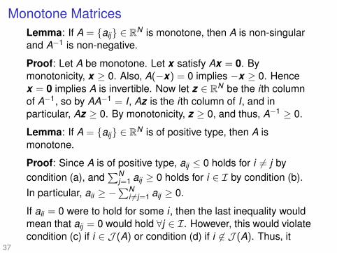
Monotone MatricesLemma: If A = aij ∈ RN is monotone, then A is non-singularand A−1 is non-negative.
Proof: Let A be monotone. Let x satisfy Ax = 0. Bymonotonicity, x ≥ 0. Also, A(−x) = 0 implies −x ≥ 0. Hencex = 0 implies A is invertible. Now let z ∈ RN be the i th columnof A−1, so by AA−1 = I, Az is the i th column of I, and inparticular, Az ≥ 0. By monotonicity, z ≥ 0, and thus, A−1 ≥ 0.
Lemma: If A = aij ∈ RN is of positive type, then A ismonotone.
Proof: Since A is of positive type, aij ≤ 0 holds for i 6= j bycondition (a), and
∑Nj=1 aij ≥ 0 holds for i ∈ I by condition (b).
In particular, aii ≥ −∑N
i 6=j=1 aij ≥ 0.
If aii = 0 were to hold for some i , then the last inequality wouldmean that aij = 0 would hold ∀j ∈ I. However, this would violatecondition (c) if i ∈ J (A) or condition (d) if i 6∈ J (A). Thus, it
37

Monotone Matricesfollows that aii > 0, i ∈ I.
Now suppose that x ∈ RN is such that Ax ≥ 0. It will be shownthat x ≥ 0. Componentwise, Ax ≥ 0 is written as
aiixi +N∑
i 6=j=1
aijxj ≥ 0, i ∈ I.
Since aij ≤ 0, i 6= j ,
aiixi −N∑
i 6=j=1
|aij |xj ≥ 0, i ∈ I
and since aii > 0,
xi ≥N∑
i 6=j=1
|aij |xj/aii , i ∈ I.
Now let r ∈ I be chosen so that xr ≤ xi , i ∈ I. It will be shownthat xr ≥ 0, which implies x ≥ 0.
Assume that xr < 0. Let first r ∈ J (A). Then the general38

Monotone Matricesestimate of xi above gives,
xr ≥N∑
r 6=j=1
|arj |xj/arr ≥N∑
r 6=j=1
|arj |xr/arr
or by dividing by xr < 0,
arr ≤N∑
r 6=j=1
|arj |.
However, if r ∈ J (A), then condition (c) meansN∑
j=1
arj > 0 and thusN∑
r 6=j=1
arj > −arr
or with condition (a) and the previous estimate of arr ,
arr >
N∑r 6=j=1
|arj | ≥ arr
a contradiction. So if xr < 0, then r 6∈ J (A). Then by condition(d), ∃ar ,k1 6= 0. It will be shown that xr = xk1 . By condition (d),39

Monotone Matrices
k1 6= r . If xk1 > xr = minxi, then by the general estimate of xi ,
arr xr ≥N∑
r ,k1 6=j=1
|arj |xj + |ar ,k1 |xk1 >
N∑r ,k1 6=j=1
|arj |xr + |ar ,k1 |xr
or by dividing by xr < 0,
arr <
N∑r 6=j=1
|arj | = −N∑
r 6=j=1
arj
which contradicts condition (b). Hence, xr = xk1 . Arguingsimilarly as if k1 were r , we find for the connectionar ,k1 ,ak1,k2 , . . . ,akm,j in A from r to j ∈ J (A) thatxr = xk1 = xk2 = · · · = xkm = xj .
However, as it was shown that for xr < 0 to hold it must be thatr 6∈ J (A), the same argument can be applied to xj = xr < 0 toconclude the necessity of j 6∈ J . The contradiction implies thatminxi = xr ≥ 0 or x ≥ 0, and hence A is monotone.
40

Existence of a Discrete Solution
Theorem: The finite difference scheme (8) has a uniquesolution.
Proof: Let d = #Ωh. The scheme (8) is an d × d system oflinear equations AhUh = Fh, where Uh ∈ Rd is a vector ofvalues of U on Ωh, Ah ∈ Rd×d is a matrix independent of f , gand u(s) and Fh ∈ Rd depends upon u(s) and grid values of fand g. It will be shown that Ah is of positive type.
To see that condition (a) is satisfied, consider first the rows i ofAh = aij corresponding to p ∈ Ωh ∪ Ω?
h\s. For these, theequations of (8) are
−∆hU(p) = f (p)for which the off-diagonal elements are ≤ 0, the non-trivial onescorresponding to Nh(p) or N?
h(p) being negative. For the row icorresponding to p = s, aii = 1 and aij = 0, j 6= i . For the rows icorresponding to p ∈ ∂Ωh, the equations of (8) are
41

Monotone Matrices
(b1 + b2)U(p)− b1U(p1)− b2U(p2) = g(p)where b1,b2 > 0. Thus, condition (a) is satisfied.
To see that condition (b) is satisfied, note that ifp ∈ Ωh ∪ Ω?
h\s, the corresponding row in Ah has sum ofelements zero. Specifically, for p ∈ Ωh, checking the sum in (3)gives (4− 1− 1− 1− 1)/h2 = 0. For p ∈ Ω?
h a zero-sum is alsoobtained from the Shortley-Weller formula (4). For p ∈ ∂Ωh azero-sum is obtained from the above approximation to thenormal derivative. For p = s, the sum of elements is∑N
j=1 aij = aii = 1.
Now let J (Ah) consist solely of the index k corresponding tothe point s. Then condition (c) is satisfied according to theequation above.
To see that condition (d) is satisfied, let p be a pointcorresponding to any index i 6= k . Then the existence of a
42

Convergence of the Discrete Solutionconnection
ai,k1 ,ak1,k2 , . . . ,aakm,kin Ah between i 6= k and k = J (Ah) is equivalent to theexistence of a zig-zag path moving horizontally or verticallyamong grid points in Ωh from the point p to the point s.Exercise: The existence of such a path follows with hsufficiently small from the assumption that Ω is connected.Thus, Ah is of positive type.
By Lemmas 37 , Ah is monotone and hence non-singular.
I The convergence U → u as h→ 0 can be shown, but thefollowing convergence estimate is stated here without proof.
Theorem: Suppose the solution u to (7) satisfies u ∈ C3(Ω).Let U be the solution to (8). Then
max(x ,y)∈Ωh
|u(x , y)− U(x , y)| ≤ c(u)h| log(h)|
where the constant c(u) depends upon u but not upon h.43

Elliptic BVPs with Variable CoefficientsI We now seek an approximation of the solution u to the
Elliptic BVP with variable coefficients,[Lu](x , y) = f (x , y), for (x , y) ∈ Ω
u(x , y) = g(x , y), for (x , y) ∈ ∂Ω(9)
where[Lu](x , y) = −∇ · [a1(x , y)∇u(x , y)] + a0(x , y)u(x , y)
I The coefficients are assumed to be sufficiently regular andto satisfy
a1(x , y) ≥ α1 > 0, a0(x , y) ≥ α0 ≥ 0, ∀(x , y) ∈ ΩI The data f and g are assumed to be sufficiently regular.I Similarly we could consider the Neumann boundary
condition ∂nu = g.I Another standard boundary condition is given by the Robin
boundary condition σ1∂nu + σ0u = g with σ1, σ0 ≥ 0 andσ1 + σ0 > 0.
I In applications, mixed problems also arise in whichdifferent boundary conditions are imposed on differentparts of ∂Ω, e.g., with σ1 or σ0 vanishing at points in ∂Ω.
44

Elliptic BVPs with Variable CoefficientsI To approximate (9) let Ωh be defined as in (2).I For p = (x , y) ∈ Ωh define Lh ≈ L by by adapting (3),
[Lhv ](x , y) = −h−2a1(x + 12h, y) [v(x + h, y)− v(x , y)]
−a1(x − 12h, y) [v(x , y)− v(x − h, y)]
+a1(x , y + 12h) [v(x , y + h)− v(x , y)]
− a1(x , y − 12h) [v(x , y)− v(x , y − h)]
+a0(x , y)v(x , y)I For p = (x , y) ∈ Ω?
h define Lh by adapting (4),
[Lhv ](x , y) = − 2h2
a1(x + 1
2γh, y)
αγ(α + γ)[αv(x + γh, y)− (α + γ)v(x , y)]
−a1(x − 1
2αh, y)
αγ(α + γ)[(α + γ)v(x , y)− γv(x − αh, y)]
+a1(x , y + 1
2δh)
βδ(β + δ)[βv(x , y + δh)− (β + δ)v(x , y)]
−a1(x , y − 1
2βh)
βδ(β + δ)[(β + δ)v(x , y)− δv(x , y − βh)]
+a0(x , y)v(x , y)45

Finite Difference SchemeI We now define the finite difference scheme approximating
the solution to the Elliptic BVP with variable coefficients:LhU(x , y) = f (x , y), for (x , y) ∈ Ωh ∪ Ω?
hU(x , y) = g(x , y), for (x , y) ∈ ∂Ωh
(10)
I Let d = #(Ωh ∪ Ω?h). The above problem (10) corresponds
to a d × d system of linear equations AhUh = Fh, whereUh ∈ Rd contains values of U on Ωh ∪ Ω?
h, Ah ∈ Rd×d is amatrix independent of f and g and Fh ∈ Rd depends upongrid values of f and g.
I Let J (Ah) consist of the indices for p ∈ Ω?h.
I Using the above matrix methods it can be shown that Ah isof positive type, hence monotone, hence invertible, andtherefore:
Theorem: The finite difference scheme (10) has a unique solution.I Convergence U → u for h→ 0 can be shown using
methods similar to those shown above.46

Non-Linear Elliptic BVPI Suppose a membrane is fastened to a boundary ∂Ω and
stretched over the interior of Ω with tension T (x , y) (forceper unit length). (figure forthcoming)
I Let u(x , y) be the displacement of the membrane resultingfrom an externally applied force per unit area f (x , y).
I The variational principle used to model the shape of themembrane involves to minimize the following energy withrespect to u:
J(u) =
∫Ω
T (x , y)√
1 + |∇u(x , y)|2dxdy−∫
Ωf (x , y)u(x , y)dxdy
I The first term involves an increase in surface area whichrepresents the elastic energy available for work to opposethe work performed by the external load as represented inthe second term.
I Using the approximation√
1 + ε2 − 1 ≈ 12ε
2, the first integrandabove may be approximated by T
2 |∇u|2 for |∇u| 1. Thenthe minimizing u satisfies a Poisson equation (u|∂Ω = 0).
47

Non-Linear Elliptic BVPI Without assuming |∇u| 1, let v ∈ C∞0 (Ω) and
δJδu
(u; v) =
∫Ω
T∇u · ∇v√1 + |∇u|2
−∫
Ωfv =
−∫
Ωv
[∇ ·
(T
∇u√1 + |∇u|2
)+ f
]+
∫∂Ω
vn·
(T
∇u√1 + |∇u|2
)I The necessary optimality condition for a minimizing u is −∇ ·
(T√
1 + |∇u|2∇u
)= f , in Ω
u = 0, on ∂Ω
(11)
I A common approach to solving such a problem is to usethe method of lagged diffusivity, where u0 = 0 and for l ∈ Nthe non-linear coefficient is replaced by T/
√1 + |∇ul−1|2
while the displacement is otherwise replaced by ul .I For each l the linear PDE can be solved by treating
T/√
1 + |∇ul−1|2 as a variable coefficient.48

Dirichlet Poisson BVP on a SquareI The solution to (1) is approximated by solving:
−∆hU(x , y) = f (x , y), for (x , y) ∈ ΩhU(x , y) = g(x , y), for (x , y) ∈ ∂Ωh
(12)
now for Ω = (0,1)2 and for N ∈ N, h = 1/(N + 1), Ω?h = ∅ and
Ωh = (x , y) : x = ih, y = jh,0 ≤ i , j ≤ N + 1.I Let d = #Ωh = N2. The above problem (12) corresponds to a
d × d system of linear equations AhUh = Fh, where Uh ∈ Rd isa vector of values of U on Ωh, Ah ∈ Rd×d is a matrix independ-ent of f and g and Fh ∈ Rd depends upon grid values of f and g.
I For simplicity let g = 0. Exercise: Generalize to g 6= 0.I Let the unknowns be ordered according to the so-called
lexicographic ordering: (figure forthcoming)Uh = U(x1, y1),U(x2, y1), . . . ,U(xN , y1),
U(x1, y2),U(x2, y2), . . . ,U(xN , y2),. . . ,U(x1, yN),U(x2, yN), . . . ,U(xN , yN)>
I The vector Fh is given by the values of f in Ωh in thelexicographic ordering.49

Dirichlet Poisson BVP on a SquareI Then the matrix Ah is given explicitly by
Ah =1h2
A1 A0A0 A1 A0
. . .. . .
. . .
A0 A1 A0A0 A1
,A0 =−I,
A1 =
4 −1−1 4 −1
. . .. . .
. . .
−1 4 −1−1 4
I (sparse!) Matlab commands for solving (12) are
B1 = speye(N); h=1/(N+1);B0 = spdiags(kron([1,1],ones(N,1)),[-1,1],N,N);A0 = -B1;A1 = spdiags(kron([-1,4,-1],ones(N,1)),[-1,0,+1],N,N);Ah = (kron(B0,A0)+kron(B1,A1))/hˆ2;Uh = zeros(N+2,N+2);Uh(2:(N+1),2:(N+1)) = reshape(Ah \ Fh,N,N);
Exercise: Implement and estimate the convergence order.50

Neumann Poisson BVP on a SquareI The solution to (7) is approximated by solving:
−∆hU(x , y) = f (x , y), for (x , y) ∈ Ωh−∆hU(x , y)+ f (x , y)+∂n,hU(x , y)/h = g(x , y)/h, for (x , y) ∈ ∂Ωh∑
(x ,y)∈ΩhU(x , y) = 0
(13)
now for Ω = (0,1)2 and for N ∈ N, h = 1/(N + 1), Ω?h = ∅ and
Ωh = (x , y) : x = ih, y = jh,0 ≤ i , j ≤ N + 1.I Also in contrast to (8), ∂n,h can be computed here more simply
and then integrated into the discrete Laplacian as seen below.I Exercise: For (xi , yj) ∈ ∂Ωh with xi = 0, and otherwise
xi = ih, the normal derivative can be approximated as
g(x0, yj)=∂nu(x0, yj)=−∂xu(x0, yj)=−[u(x0, yj)−u(x−1, yj)]/h+O(h)
I The normal derivative can also be approximated as
g(x0, yj)=∂nu(x0, yj)=−∂xu(x0, yj)=−[u(x1, yj)−u(x−1, yj)]/(2h)+O(h2)
which leads to a non-symmetric matrix Ah.51

Neumann Poisson BVP on a SquareI Integrating the O(h) approximation to ∂n into ∆hU gives,
f (x0, yj) = −∆hU(x0, yj) =h−2[U(x0, yj)− U(x−1, yj)]− [U(x1, yj)− U(x0, yj)]
+[U(x0, yj+1)− U(x0, yj)]− [U(x0, yj)− U(x0, yj−1)]= h−2−hg(x0, yj)− [U(x1, yj)− U(x0, yj)]
+[U(x0, yj+1)− U(x0, yj)]− [U(x0, yj)− U(x0, yj−1)]and similarly for other points on ∂Ωh.
I Let d = #Ωh = (N + 2)2. The above problem (13)corresponds to a d × d system of linear equationsAhUh = Fh, where Uh ∈ Rd is a vector of values of U onΩh, Ah ∈ Rd×d is a matrix independent of f and g andFh ∈ Rd depends upon grid values of f and g.
I For simplicity let g = 0. Exercise: Generalize to g 6= 0.I Let the unknowns Uh be ordered by the lexicographic
ordering.I The vector Fh is given by the values of f in Ωh in the
lexicographic ordering.52

Neumann Poisson BVP on a Square
I Then the matrix Ah is given explicitly by
Ah =1h2
A1 A0A0 A2 A0
. . .. . .
. . .
A0 A2 A0A0 A1
with A0 = −I and
A1 =
2 −1−1 3 −1
. . .. . .
. . .
−1 3 −1−1 2
A2 =
3 −1−1 4 −1
. . .. . .
. . .
−1 4 −1−1 3
53

Neumann Poisson BVP on a SquareI The additional condition in (13) that
∑(x ,y)∈Ω U(x , y) = 0
corresponds to selecting the solution to (7) with meanvalue zero. Such a solution (with g = 0) is stationary forthe Lagrangian functional,
L(u) =
[∫Ω
12 |∇u|2 −
∫Ω
fu]
+ λ
∫Ω
u
where λ is a Lagrange multiplier corresponding to thecondition
∫Ω u = 0.
I Exercise: The stationarity conditions for L are
−∆u + λ = f in Ω, ∂nu = 0 on ∂Ω, and∫
Ωu = 0.
I With e = (1,1, . . . ,1)> ∈ Rd the discrete counterpart tothese stationarity conditions is[
Ah ee> 0
] [Uhλ
]=
[Fh0
]where the last component of this system is seen as thecondition
∑(x ,y)∈Ω U(x , y) = 0.
54

Neumann Poisson BVP on a Square
I (sparse!) Matlab commands for solving (13) areN1=N+1; N2=N+2; N2N2 = N2*N2; h=1/N1;B1=sparse(N2,N2); B1(1,1) = 1; B1(N2,N2) = 1;B2=speye(N2,N2); B2(1,1) = 0; B2(N2,N2) = 0;B0=spdiags(kron([1,1],ones(N2,1)),[-1,1],N2,N2);A0=-speye(N2);A1=spdiags(kron([-1,3,-1],ones(N2,1)),[-1,0,+1],N2,N2);
A1(1,1) = 2; A1(N2,N2) = 2;A2=spdiags(kron([-1,4,-1],ones(N2,1)),[-1,0,+1],N2,N2);
A2(1,1) = 3; A3(N2,N2) = 3;Ah=kron(B0,A0)+kron(B1,A1)+kron(B2,A2);Ah=Ah/hˆ2;e =ones(N2N2,1); Uh=[Ah,e;e’,0] \ [Fh;0];Uh=reshape(Uh(1:N2N2),N2,N2);
Exercise: Implement and estimate the convergence order.What happens if e’*Fh =/= 0 ?
55

Non-Linear Elliptic BVP on a SquareI To solve the non-linear elliptic BVP (11) on Ω = (0,1)2 we
set w0 = 0 and for a given l ∈ N we seek an approximationto the solution wl of the now linear elliptic BVP, −∇ ·
(T√
1 + |∇wl−1|2∇wl
)= f , in Ω
wl = 0, on ∂Ω
(14)
I Setting u = wl and
al(x , y) =T (x , y)√
1 + |∇wl−1(x , y)|2≥ min
(x ,y)∈ΩT (x , y) > 0
permits (14) to be formulated like (9), an elliptic BVP withvariable coefficients,
[Llu](x , y) = f (x , y), for (x , y) ∈ Ωu(x ,0) = 0, for (x , y) ∈ ∂Ω
(15)
where[Llu](x , y) = −∇ · [al(x , y)∇u(x , y)]
56

Non-Linear Elliptic BVP on a SquareI To approximate (15) let Ωh and Lh,l be defined as for (9) but
now with Ω?h = ∅, a1 = al and a0 = 0.
I The solution to (15) is approximated with the finitedifference scheme
[Lh,lU](x , y) = f (x , y), for (x , y) ∈ ΩhU(x , y) = 0, for (x , y) ∈ ∂Ωh
(16)
now for Ω = (0,1)2 and for N ∈ N, h = 1/(N + 1), Ω?h = ∅ and
Ωh = (x , y) : x = ih, y = jh,0 ≤ i , j ≤ N + 1.I Let d = #Ωh = N2. The above problem (16) corresponds
to a d × d system of linear equations Ah,lUh = Fh, whereUh ∈ Rd is a vector of values of U on Ωh, Ah,l ∈ Rd×d is amatrix independent of f and Fh ∈ Rd depends upon gridvalues of f .
I Let the unknowns of Uh and the f -values of Fh be orderedaccording to the lexicographic ordering.
57

Non-Linear Elliptic BVP on a Square
I The formulas 45 for Lh,l require to evaluate al at midpoints(x + 1
2 ih, y + 12 jh), |i |+ |j | = 1, between grid points (x , y) ∈ Ωh,
al(x + 12 ih, y + 1
2 jh) =T (x + 1
2 ih, y + 12 jh)√
1 + |∇hv(x + 12 ih, y + 1
2 jh)|2, v = wl−1
I The gradient ∇h ≈ ∇ above is approximated compactlywith the finite differences (figure forthcoming)
∇h,xv(x + 12 ih, y) =
[[Dh,xv ](x + 1
2 ih, y)
[Ch,yv ](x + 12 ih, y)
]for i = ±1 and
∇h,yv(x , y + 12 jh) =
[[Ch,xv ](x , y + 1
2 jh)
[Dh,yv ](x , y + 12 jh)
]for j = ±1 where (with values understood to be 0 at ∂Ωh)
[Dh,xv ](x + 12 ih, y) = [v(x + ih, y)− v(x , y)] /h
[Dh,yv ](x , y + 12 jh) = [v(x , y + jh)− v(x , y)] /h
58

Non-Linear Elliptic BVP on a Squareand (with values understood to be 0 at ∂Ωh)
[Ch,xv ](x , y + 12 jh) =
14h
(v(x + h, y) + v(x + h, y + jh)−v(x − h, y)− v(x − h, y + jh)
)[Ch,yv ](x + 1
2 ih, y) =1
4h
(v(x , y + h) + v(x + ih, y + h)−v(x , y − h)− v(x + ih, y − h)
)I The matrix representations of these operators are
Dh,x =
D1. . .
D1
, D1 =1h
1−1 1
. . .. . .
−1 1−1
Dh,y =1h
D0−D0 D0
. . .. . .
−D0 D0−D0
, D0 =
1. . .
1
59

Non-Linear Elliptic BVP on a Squareand
Ch,x =12
C1C1 C1
. . .. . .
C1 C1C1
C1 =1
2h
0 1−1 0 1
. . .. . .
. . .
−1 0 1−1 0
Ch,y =1
2h
0 C0
−C0 0 C0. . .
. . .. . .
−C0 0 C0−C0 0
C0 =12
11 1
. . .. . .
1 11
I Set the tension values at midpoints,
Th,x = T ((i + 12)h, jh) : i = 0, . . . ,N, j = 1, . . . ,N
Th,y = T (ih, (j + 12)h) : i = 1, . . . ,N, j = 0, . . . ,N
60

Non-Linear Elliptic BVP on a SquareI Let Vh denote the vector of lexicographically ordered
values approximating wl−1 on Ωh.I Set the values of coefficients at midpoints,
al,x = Th,x ./√
1 + (Dh,xVh).ˆ2 + (Ch,yVh).ˆ2
al,y = Th,y ./√
1 + (Ch,xVh).ˆ2 + (Dh,yVh).ˆ2
I Let D(V ) denote a diagonal matrix with the values of thevector V along the diagonal.
I Then the coefficient matrix for the system of linearequations Ah,lUh = Fh for the solution to (16) is givenexplicitly by
Ah,l = D>h,xD(al,x )Dh,x + D>h,yD(al,y )Dh,yI For example, suppose the following data are given:N1 = N+1; NN1 = N*N1; h=1/N1;Fh = f0*ones(N,N); Fh = Fh(:); % f0 = ?Tx = T0*ones(N1,N); Tx = Tx(:); % T0 = ?Ty = T0*ones(N,N1); Ty = Ty(:);61

Non-Linear Elliptic BVP on a SquareI (sparse!) Matlab commands for solving (16) are
D0 = speye(N);D1 = spdiags(kron([-1,1],ones(N,1)),[-1,0],N1,N)/h;Dx = kron(D0,D1); Dy = kron(D1,D0);C0 = spdiags(kron([1,1],ones(N,1)),[-1,0],N1,N)/2;C1 = spdiags(kron([-1,1],ones(N,1)),[-1,1],N,N)/(2*h);Cx = kron(C0,C1); Cy = kron(C1,C0);Uh = zeros(N,N); Uh=Uh(:);% iterate until convergence
Vh = Uh;ax = Tx./sqrt(1 + (Dx*Vh).ˆ2 + (Cy*Vh).ˆ2);ay = Ty./sqrt(1 + (Cx*Vh).ˆ2 + (Dy*Vh).ˆ2);Ah = Dx’*spdiags(ax,0,NN1,NN1)*Dx ...
+ Dy’*spdiags(ay,0,NN1,NN1)*Dy;Uh = Ah \ Fh;% if ||Uh-Vh|| small enough, break
Exercise: Implement and show convergence w.r.t. l for f0 ≤ ?T0.62

Heat EquationI Let Ω = (0,1) and T > 0 and set Q = Ω× (0,T ).I For a given constant diffusivity α > 0 we week an
approximation of the solution u to the Heat Equation withDirichlet Boundary Conditions,
ut (x , t) = αuxx (x , t), for (x , t) ∈ Ω× (0,T ]u(x , t) = g(x , t), for (x , t) ∈ ∂Ω× [0,T ]u(x ,0) = u0(x), for (x , t) ∈ Ω× 0
(17)
I For simplicity let g = 0. Exercise: Generalize to g 6= 0.I For compatibility it must hold that u0(x) = 0, x ∈ ∂Ω.I Under this compatibility condition and with u0 ∈ C(Ω),
(17) has a unique solution in C2,1(Q), where
‖u‖Cm,n(Q) = max1≤i≤m
max1≤k≤n
sup(x ,t)∈Q
|∂ ix∂
kt u(x , t)|
and, according to a maximum principle,
max(x ,t)∈Q
|u(x , t)| ≤ maxx∈Ω|u0(x)|
63

Explicit Finite Difference SchemeI For the discretization of (17) let N,K ∈ N and set
h = 1/(N + 1), xi = ih, i = 0, . . . ,N + 1τ = T/K , tk = kτ, k = 0, . . . ,K
and adopt the notation uki = u(xi , tk ).
I A finite difference scheme for computing Uki ≈ uk
i is givenfirst by approximating the PDE according to
Uk+1i − Uk
iτ
= αUk
i+1 − 2Uki + Uk
i−1
h2
I By setting λ = ατ/h2, the IBVP (17) is approximated byUk+1
i = λUki+1 + (1− 2λ)Uk
i + λUki−1, 1 ≤ i ≤ N,1 ≤ k ≤ K − 1
Uk0 = Uk
N+1 = 0, 0 ≤ k ≤ K
U0i = u0(xi), 0 ≤ i ≤ N + 1
(18)I Setting Uk
h = Uki
Ni=1 this explicit scheme can be written as
Uk+1h − Uk
h = ατAhUkh , Ah = tridiag−1,2,−1/h2
or Uk+1h = BλUk
h , Bλ = tridiagλ,1− 2λ, λ64

Stability of Explicit SchemeI To prove convergence U → u as h, τ → 0, stability is first
established as follows.
Lemma: Let λ ∈ (0,1/2]. Then the solution Uki to (18)
satisfies max0≤i≤N+1,0≤k≤K
|Uki | ≤ max
0≤i≤N+1|u0(xi)|
Proof: By (18), for 1 ≤ i ≤ N, it follows with λ ∈ (0,1/2] that|Uk+1
i | ≤ λ|Uki+1|+ (1− 2λ)|Uk
i |+ λ|Uki−1|
≤ (λ+1−2λ+λ) max0≤i≤N+1
|Uki |
Since Uk+10 = Uk+1
N+1 = 0, the max over 0 ≤ i ≤ N + 1 can betaken on the left side of the estimate, and the claim follows.
I The restriction λ ∈ (0,1/2] is crucial here for stability.
Exercise: Construct an example for which the scheme (18)gives unbounded values Uk
i for λ > 1/2 as k ,h→ 0.
I The restriction λ ∈ (0,1/2] is severe here: τ = O(h2)!65

Consistency of Explicit SchemeI To prove convergence U → u as h, τ → 0, consistency is
next established as follows.
Lemma: Let u ∈ C4,2(Q) be the solution to (17). Then forbλuk
i := λuki+1 + (1− 2λ)uk
i + λuki−1
∃c 6= c(h, τ) such thatmax
1≤i≤N,0≤k≤K|uk+1
i − bλuni | ≤ cτ(τ + h2)‖u‖C4,0(Q)
Proof: Expanding each term of bλuki about (xi , tk ) gives
bλuki = uk
i +λh2uxx (xi , tk ) +λh4
24
[∂4u∂x4 (θi− 1
2, tk ) +
∂4u∂x4 (θi+ 1
2, tk )
]for constants θi− 1
2∈ [xi−1, xi ] and θi+ 1
2∈ [xi , xi+1]. Expanding
uk+1i about (xi , tk ) gives
uk+1i = uk
i + τut (xi , tk ) +τ2
2utt (xi , θk+ 1
2)
for a constant θk+ 12∈ [tk , tk+1]. Combining these estimates and
66

Convergence of Explicit Schemerecalling λh2 = ατ and ut = αuxx gives
uk+1i −bλuk
i =τ2
2utt (xi , θk+ 1
2)−λh4
24
[∂4u∂x4 (θi− 1
2, tk ) +
∂4u∂x4 (θi+ 1
2, tk )
]Setting utt = αuxxt = α(ut )xx = α2uxxxx proves the claim.
I Note that the stability restriction λ ∈ (0,1/2] did not enterinto the consistency proof.
I Also consistency is not equivalent to convergence, which isproved as follows by combining consistency with stability.(cf. Lax Equivalence Theorem.)
Theorem: Let u ∈ C4,2(Q) be the solution to (17). Forλ ∈ (0,1/2] let Uk
i be the solution to (18). Then ∃c 6= c(h, τ)such that
max0≤i≤N+1,0≤k≤K
|Uki − u(xi , tk )| ≤ c(τ + h2)‖u‖C4,0(Q)
67

Convergence of Explicit Scheme
Proof: Let eki = Uk
i − uki , which satisfies ek
0 = e0N+1 = 0 for
k = 0, . . . ,K and e0i = 0 for 0 ≤ i ≤ N + 1. For 1 ≤ i ≤ N and
0 ≤ k ≤ K − 1,ek+1
i = Uk+1i − uk+1
i = bλUki − uk+1
i ± bλuki
= bλeki + (bλuk
i − uk+1i )
Since λ ∈ (0,1/2], ek+1i depends stably upon ek
i ,
|ek+1i | ≤ λ|ek
i+1|+ (1− 2λ)|eki |+ λ|ek
i−1|+ |bλuki − uk+1
i |and using the consistency estimate,
max1≤i≤N
|ek+1i | ≤ max
1≤i≤N|ek
i |+ cτ(τ + h2)‖u‖C4,0(Q)
Summing this estimate over k = 0, . . . , κ− 1, κ ≤ K , gives
max1≤i≤N
|eκi | ≤ max1≤i≤N
|e0i |+ cκτ(τ + h2)‖u‖C4,0(Q)
Setting c = cT (≥ cκτ) and recalling where eki vanishes gives
the claimed convergence estimate.68

Neumann Heat Equation on a SquareI Let Ω = (0,1)2 and T > 0.I For a given constant diffusivity α > 0 we week an
approximation of the solution u to the Heat Equation withNeumann Boundary Condition,
ut (x , y , t) = α∆u(x , y , t), for (x , y , t) ∈ Ω× (0,T ]∂nu(x , y , t) = g(x , y , t), for (x , y , t) ∈ ∂Ω× [0,T ]
u(x , y ,0) = u0(x , y), for (x , y , t) ∈ Ω× 0(19)
I For simplicity let g = 0. Exercise: Generalize to g 6= 0.I For compatibility it must hold that ∂nu0(x , y) = 0, x ∈ ∂Ω.I Let the Laplacian ∆ be approximated with Neumann
boundary conditions as was done for the Poisson equationon a square in (13).
I With Ωh and Ah defined as for 53 , (19) can be semi-discretizedspatially by the system of ODEs (method of lines),
U ′h(t) = −αAhUh(t), Uh(0) = U0 = u0(xi , yj), Uh(t) = Ui,j(t)69

Semi-Discrete SolutionI This semi-discrete solution Uh(t) has the property
12Dt‖Uh(t)‖2 = Uh(t) · U ′h(t) = −αUh(t) · [AhUh(t)] ≤ 0
which implies ‖Uh(t)‖ ≤ ‖U0‖, analogous to the estimatefor the solution u to (19),12Dt
∫Ω
u2 =
∫Ω
uut =
∫Ωαu∆u =
∫∂Ωαu∂nu−
∫Ωα|∇u|2 ≤ 0
I Also Uh(t) satisfiese · U ′h(t) = −αe · [AhUh(t)] = −α[Ahe] · Uh(t) = 0
which implies e · U ′h(t) = e · U0, analogous to the estimatefor the solution u to (19),
12Dt
∫Ω
u =
∫Ω
ut =
∫Ωα∆u =
∫∂Ωα∂nu = 0
I Exercise: The fully-discrete explicit Euler scheme,Uk+1
h − Ukh = ταAhUk
h , Ukh = Uk
i,j, Uki,j ≈ u(xi , yj , tk )
satisfies the property e · Ukh = e · U0
h but it satisfies‖Uk
h ‖ ≤ ‖U0h‖ only for λ = ατ/h2 ≤ 1/4.
70

Explicit and Implicit Euler SchemesI Exercise: The implicit Euler scheme
Uk+1h − Uk
h = −ταAhUk+1h , [I + ατAh]Uk+1
h = Ukh
satisfies the conditione · Uk+1
h = e · [I + ατAh]Uk+1h = e · Uk
h
or e · Ukh = e · U0, and furthermore
‖Uk+1h ‖2 ≤ Uk+1
h ·[I+ατAh]Uk+1h = Uk+1
h ·Ukh ≤ ‖U
k+1h ‖‖Uk
h ‖
or, analogous to 65 , ‖Ukh ‖ ≤ ‖U
0h‖ holds but now without
conditions on τ or h.I Exercise: Analogous to 66 , show that the implicit Euler
scheme is consistent to O(τ(τ + h2)).I Exercise: Analogous to 67 , show that the implicit Euler
scheme is convergent with convergence rate O(τ + h2).I (sparse!) Matlab commands for solving (19) (Ah from 55 ,Uh = U0 given) are
for k=1:K Uh = (speye(N2N2)+al*ta*Ah) \ Uh; end71

Non-Linear Parabolic IBVPI Let f : Ω→ [0,1] be a measured image defined on
Ω = (0,1)2 which is to be denoised.I The steepest descent evolution,∫
Ωutv = −δJ
δu(u; v), u|t=0 = f , t ∈ [0,T ], v ∈ C∞(Ω)
produces a sequence of images u which start at f andbecome progressively less noisy as time advances.
I The descent direction reduces a regularizer such as
J(u) = α
∫Ω
√ε+ |∇u|2
Here, J(u)→ αTV(u) for ε→ 0 and u sufficiently smooth.I For the explicit form of the evolution, let v ∈ C∞(Ω) and
0 =
∫Ω
utv +δJδu
(u; v) =
∫Ω
[vut + α
∇u · ∇v√ε+ |∇u|2
]=
∫Ω
v
[ut −∇ ·
(α
∇u√ε+ |∇u|2
)]+
∫∂Ω
vn·
(α
∇u√ε+ |∇u|2
)72

Non-Linear Anisotropic DiffusionI The steepest descent evolution is given explicitly by the
resulting non-linear anisotropic diffusion equation,ut = α∇ ·
(∇u√
ε+ |∇u|2
), in Ω× (0,T ]
∂nu = 0, on ∂Ω× [0,T ]
u = f , in Ω× 0
(20)
I To approximate the solution, (20) is first discretizedtemporally with a semi-implicit Euler scheme to obtain
Lkuk = uk−1, in Ω
∂nuk = 0, on ∂Ω
k = 1, . . . ,Ku0 = f
(21)
where T = K τ and
Lku = u − τ∇ · (ak∇u) , ak =α√
ε+ |∇uk−1|2
I To approximate the solution to (21) spatially, let Ωh and Lh,kbe defined as for (9) but now with Ω?
h = ∅, a1 = ak and a0 = 1.73

Fully Discrete ApproximationI The solution to (21) is approximated spatially with the finite
difference schemeLh,kUk = Uk−1, in Ωh
Lh,kUk + ak∂n,hUk/h = Uk−1, in ∂Ωh(22)
now for Ω = (0,1)2 and for N ∈ N, h = 1/(N + 1), Ω?h = ∅ and
Ωh = (x , y) : x = ih, y = jh,0 ≤ i , j ≤ N + 1.I Let d = #Ωh = (N + 2)2. The above problem (22)
corresponds to a d × d system of linear equationsAh,kUk
h = Uk−1h , where Uk
h ∈ Rd is a vector of values of Uk
on Ωh and Ah,k ∈ Rd×d is a matrix depending upon ak andhence Uk−1.
I Let the unknowns of Ukh be ordered according to the
lexicographic ordering.I The formulas 45 for Lh,k require to evaluate ak at midpoints
(x + 12 ih, y + 1
2 jh), |i |+ |j | = 1, between grid points (x , y) ∈ Ωh,74

Approximation of Non-Linear Coefficients
ak (x + 12 ih, y + 1
2 jh) =α√
1 + |∇hUk−1(x + 12 ih, y + 1
2 jh)|2
I The gradient ∇h ≈ ∇ above is approximated compactlywith the finite differences (figure forthcoming)
∇h,xv(x + 12 ih, y) =
[[Dh,xv ](x + 1
2 ih, y)
[Ch,yv ](x + 12 ih, y)
]for i = ±1 and
∇h,yv(x , y + 12 jh) =
[[Ch,xv ](x , y + 1
2 jh)
[Dh,yv ](x , y + 12 jh)
]for j = ±1 where
[Dh,xv ](x + 12 ih, y) = [v(x + ih, y)− v(x , y)] /h
[Dh,yv ](x , y + 12 jh) = [v(x , y + jh)− v(x , y)] /h
75

Approximation of the Gradientand (with difference quotients [υ(z + h)− υ(z − h)]/(2h)
replaced by [υ(z + h)− υ(z)]/h for z − h < 0or by [υ(z)− υ(z − h)]/h for z + h > 1)
[Ch,xv ](x , y + 12 jh) =
14h
(v(x + h, y) + v(x + h, y + jh)−v(x − h, y)− v(x − h, y + jh)
)[Ch,yv ](x + 1
2 ih, y) =1
4h
(v(x , y + h) + v(x + ih, y + h)−v(x , y − h)− v(x + ih, y − h)
)I The matrix representations of these operators are
Dh,x =
D1. . .
D1
, D1 =1h
−1 1. . .
. . .
−1 1
Dh,y =1h
−D0 D0. . .
. . .
−D0 D0
, D0 =
1. . .
1
76

Approximation of the Gradient
and
Ch,x =12
C1 C1. . .
. . .
C1 C1
C1 =1
2h
−2 2−1 0 1
. . .. . .
. . .
−1 0 1−2 2
Ch,y =1
2h
−2C0 2C0−C0 0 C0
. . .. . .
. . .
−C0 0 C0−2C0 2C0
C0 =12
1 1. . .
. . .
1 1
Exercise: Derive these explicit formulas for Dh,x ,Dh,y ,Ch,x ,Ch,yas well as the counterparts for (14) and highlight thedifferences resulting from the respective boundary conditions.
77

Approximation of Non-Linear OperatorI Set the values of coefficients at midpoints,
ak ,x = α./√ε+ (Dh,xUk−1
h ).ˆ2 + (Ch,yUk−1h ).ˆ2
ak ,y = α./√ε+ (Ch,xUk−1
h ).ˆ2 + (Dh,yUk−1h ).ˆ2
I Let D(V ) denote a diagonal matrix with the values of thevector V along the diagonal.
I With [D>h,x ,D>h,y ] = ∇>h ≈ (∇)∗ = −∇·, the coefficient
matrix Ah,k in Ah,kUkh = Uk−1
h for the solution to (22) isgiven explicitly by
Ah,k = I + τ[D>h,xD(ak ,x )Dh,x + D>h,yD(ak ,y )Dh,y
]I For example, suppose the following data are given:
N1 = N+1; h=1/N1; ta = T/M;N2 = N+2; N1N2 = N1*N2; N2N2 = N2*N2; N4 = N2/4;Fh = [zeros(N4,1);ones(N2-2*N4,1);zeros(N4,1)];Fh = reshape(Fh*Fh’ + 0.5*randn(N2,N2),N2N2,1);78

Code to Solve the Non-Linear IBVPI (sparse!) Matlab commands for solving (22) are
D0 = speye(N2);D1 = spdiags(kron([-1,1],ones(N2,1)),[0,1],N1,N2)/h;Dx = kron(D0,D1); Dy = kron(D1,D0);C0 = spdiags(kron([1,1],ones(N2,1)),[0,1],N1,N2)/2;C1 = spdiags(kron([-1,1],ones(N2,1)),[-1,1],N2,N2)/(2*h);C1(1,1) = -1/h; C1(1,2) = 1/h;C1(N2,N2-1) = -1/h; C1(N2,N2) = 1/h;Cx = kron(C0,C1); Cy = kron(C1,C0);Uh = Fh; I = speye(N2N2);for k=1:K
ax = al./sqrt(ep + (Dx*Uh).ˆ2 + (Cy*Uh).ˆ2);ay = al./sqrt(ep + (Cx*Uh).ˆ2 + (Dy*Uh).ˆ2);Ah = I + ta*(Dx’*spdiags(ax,0,N1N2,N1N2)*Dx ...
+ Dy’*spdiags(ay,0,N1N2,N1N2)*Dy);Uh = Ah \ Uh;
endExercise: Implement and estimate best ε, α and T .79

Wave EquationI Let Ω = (0,1) and T > 0 and set Q = Ω× (0,T ).I For a given constant wave speed ω > 0 we week an
approximation of the solution u to the Wave Equation withDirichlet Boundary Conditions,
utt (x , t) = ω2uxx (x , t), for (x , t) ∈ Ω× (0,T ]u(x , t) = g(x , t), for (x , t) ∈ ∂Ω× [0,T ]u(x ,0) = u0(x), for (x , t) ∈ Ω× 0ut (x ,0) = u1(x), for (x , t) ∈ Ω× 0
(23)I For simplicity let g = 0. Exercise: Generalize to g 6= 0.I For compatibility it must hold that u0(x) = u1(x) = 0, x ∈ ∂Ω.I If the initial data u0 and u1 have compact support in Ω,
then, for t sufficiently small, waves do not reach ∂Ω, andthe solution is given by d’Alembert’s formula,
u(x , t) =12
[u0(x − ωt) + u0(x + ωt)] +1
2ω
∫ x+ωt
x−ωtu1(s)ds
which shows how u inherits its regularity from that of u0 and u1.80

Explicit Finite Difference SchemeI For the discretization of (23) let N,K ∈ N and set
h = 1/(N + 1), xi = ih, i = 0, . . . ,N + 1τ = T/K , tk = kτ, k = 0, . . . ,K
and adopt the notation uki = u(xi , tk ).
I A finite difference scheme for computing Uki ≈ uk
i is givenfirst by approximating the PDE according to
Uk+1i − 2Uk
i + Uk−1i−1
τ2 = ω2 Uki+1 − 2Uk
i + Uki−1
h2 ,1 ≤ i ≤ N
k = 1, . . . ,K − 1
with Uk0 = Uk
N+1 = 0, k = 0, . . . ,K , but we need U0j and U1
j .I The initial conditions begin naturally with
U0i = u0(xi), 0 ≤ i ≤ N + 1.
I For U1i note that U1
i ≈ u(xi , t1), which can be expanded as
u(xi , t1) = u(xi ,0) +τut (xi ,0) + 12τ
2utt (xi ,0) + 16τ
3uttt (xi , θ 12)
for θ 12∈ [0, τ ].
81

Initial Conditions of Explicit SchemeI Using the initial values u(x ,0) = u0(x), ut (x ,0) = u1(x)
and utt = ω2uxx the expansion gives
u(xi , t1) = u0(xi) + τu1(xi) + 12τ
2ω2u′′0(xi) +O(τ3)
I Thus for 1 ≤ i ≤ N we set
U1i = u0(xi) +τu1(xi) +
ω2τ2
2h2 [u0(xi+1)− 2u0(xi) + u0(xi−1)]
which has the following order of consistency.
Lemma: For u0 ∈ C4(Ω) and u ∈ C0,3(Q), ∃c 6= c(h, τ) suchthat
max0≤i≤N+1
|U1i − u1
i | ≤ c[τ2h2‖u0‖C4(Ω) + τ3‖u‖C0,3(Q)
]Proof: Exercise with Taylor expansions.
Def: Let r = ωτ/h be called the Courant Number.
I The finite difference scheme for approximating the solutionu to (23) is now given by the explicit method
82

Consistency of Explicit Scheme
Uk+1i = r2(Uk
i+1 + Uki−1) + 2(1− r2)Uk
i − Uk−1i
1 ≤ k ≤ K − 1,1 ≤ i ≤ NUk
0 = UkN+1 = 0, 0 ≤ k ≤ K
U0i = u0(xi), 0 ≤ i ≤ N + 1
U1i = u0(xi) + τu1(xi)+
(r2/2) [u0(xi+1)− 2u0(xi) + u0(xi−1)] ,1 ≤ i ≤ N
(24)
I This scheme is consistent according to the following.
Lemma: Let u ∈ C4,2(Q) be the solution to (23). Then∃c 6= c(h, τ) such that
max1≤i≤N,0≤k≤K
|uk+1i − [r2(uk
i+1 + uki−1) + 2(1− r2)uk
i − uk−1i ]|
≤ cτ2(τ2 + h2)‖u‖C4,0(Q)
Proof: Exercise with Taylor expansions.83

Forward, Backward, Centered DifferencesI Now some standard notation:
∆vi = vi+1 − vi , forward difference∇vi = vi − vi−1, backward differenceδvi = vi+ 1
2− vi− 1
2, central difference
and it holds that∆∇vi = vi+1 − 2vi + vi−1 = δδvi .
I On the subspace V0 = viN+1i=0 : v0 = vN+1 = 0 ⊂ RN+2
define the bilinear formah(v ,w) = −h
N∑i=1
(∆∇vi)wi (25)
Lemma: It holds thata. ∀v ,w ∈ V0,
ah(v ,w) = ah(w , v) = hN+1∑i=1
(∇vi)(∇wi)
b. ∀v ∈ V0,ah(v , v) ≥ 0 and ah(v , v) = 0 ⇒ v = 0.
c. By (1) and (2), ah(v ,w) is an inner product on V0 giving anorm ah(v , v)
12 so that ∀v ,w ∈ V0,
84

Bilinear Form|ah(v ,w)| ≤ ah(v , v)
12 ah(w ,w)
12
d. ∀v ∈ V0,ah(v , v)
12 ≤ 2‖v‖h, ‖v‖2h = h
N∑i=1
v2i
Proof: Exercise
Theorem: Let u ∈ C4,3(Q) be the solution to (23). Let Uki be
the solution to (24). Then for each r0 ∈ (0,1), ∃c = c(r0,T )such that for r = ωτ/h, 0 < r ≤ r0,
max0≤k≤K
‖Ukh − uk‖h ≤ c(h2 + τ2)‖u‖C4,3(Q)
Proof: Set eki = Uk
i − uki , 0 ≤ i ≤ N + 1, and note that
ek0 = ek
N+1 = 0. Set also ekh = ek
i N+1i=0 and note that ek
h ∈ V0.Then for 1 ≤ i ≤ N, 1 ≤ k ≤ K − 1,
ek+1i −2ek
i +ek−1i = (Uk+1
i −2Uki +Uk−1
i )− (uk+1i −2uk
i +uk−1i )
= r2(Uki+1−2Uk
i +Uki−1)±r2(uk
i+1−2uki +uk
i−1)−(uk+1i −2uk
i +uk−1i )
85

Convergence of Explicit Schemeor
ek+1i − 2ek
i + ek−1i = r2(ek
i+1 − 2eki + ek
i−1) + εki
whereεk
i = r2(uki+1 − 2uk
i + uki−1)− (uk+1
i − 2uki + uk−1
i )
Multiplying the last e-equation by h(ek+1i − ek−1
i ) and summingover i = 1, . . . ,N gives
hN∑
i=1
(ek+1i − 2ek
i + ek−1i )(ek+1
i − ek−1i ) =: L = R1 + R2 :=
r2hN∑
i=1
(eki+1 − 2ek
i + eki−1)(ek+1
i − ek−1i ) + h
N∑i=1
εki (ek+1
i − ek−1i )
Then
L = hN∑
i=1
[(ek+1i − ek
i )− (eki − ek−1
i )][(ek+1i − ek
i ) + (eki − ek−1
i )] =
hN∑
i=1
(ek+1i − ek
i )2 − hN∑
i=1
(eki − ek−1
i )2 = ‖ek+1h − ek
h‖2h − ‖e
kh − ek−1
h ‖2h
86

Convergence of Explicit Schemeand with (25) and property (a) in Lemma 84 ,
R1 = −r2ah(ekh ,e
k+1h − ek−1
h ) = −r2ah(ekh ,e
k+1h ) + r2ah(ek
h ,ek−1h ) =
−12 r2[ah(ek+1
h ,ek+1h )− ah(ek−1
h ,ek−1h )
]+1
2 r2[ah(ek+1
h − ekh ,e
k+1h − ek
h)− ah(ekh − ek−1
h ,ekh − ek−1
h )]
Using these calculations to rewrite L = R1 + R2 gives
‖ek+1h − ek
h‖2h − ‖e
kh − ek−1
h ‖2h+1
2 r2[ah(ek+1
h ,ek+1h )± ah(ek
h ,ekh)− ah(ek−1
h ,ek−1h )
]−1
2 r2[ah(ek+1
h − ekh ,e
k+1h − ek
h)− ah(ekh − ek−1
h ,ekh − ek−1
h )]
= hN∑
i=1
εki (ek+1
i − ek−1i )
Summing over k = 1, . . . , κ− 1, κ ≤ K , and observing e0h = 0
87
Convergence of Explicit Schemegives[‖eκh − eκ−1
h ‖2h − ‖e1h‖
2h ± 1
2 r2ah(e1h,e
1h)]
+12 r2[ah(eκh ,e
κh) + ah(eκ−1
h ,eκ−1h )− ah(eκh − eκ−1
h ,eκh − eκ−1h )
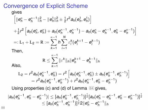
]=: L1 + L2 = R :=
κ−1∑k=1
hN∑
i=1
εki (ek+1
i − ek−1i )
Then,
R ≤κ−1∑k=1
‖εk‖h‖ek+1h − ek−1
h ‖hAlso,
L2 = r2ah(eκ−1h ,eκh) = r2
[ah(eκ−1
h ,eκh)± ah(eκ−1h ,eκ−1
h )]
= r2ah(eκ−1h ,eκ−1
h ) + r2ah(eκ−1h ,eκh − eκ−1
h )
Using properties (c) and (d) of Lemma 84 gives,
|ah(eκ−1h ,eκh − eκ−1
h )| ≤ [ah(eκ−1h ,eκ−1
h )]12 [ah(eκh − eκ−1
h ,eκh − eκ−1h )]
12
≤ [ah(eκ−1h ,eκ−1
h )]12 2‖eκh − eκ−1
h ‖h88

Convergence of Explicit SchemeUsing 2ab ≤ a2 + b2, the last inequality becomes
|ah(eκ−1h ,eκh − eκ−1
h )| ≤ ah(eκ−1h ,eκ−1
h ) + ‖eκh − eκ−1h ‖2h
and hence
r2ah(eκ−1h ,eκh − eκ−1
h ) + r2ah(eκ−1h ,eκ−1
h ) ≥ −r2‖eκh − eκ−1h ‖2h
Thus, rewriting L1 + L1 = R with these calculations gives(1− r2)‖eκh − eκ−1
h ‖2h
≤ ‖eκh − eκ−1h ‖2h + r2ah(eκ−1
h ,eκ−1h ) + r2ah(eκ−1
h ,eκh − eκ−1h )
≤ ‖e1h‖
2h +
κ−1∑k=1
‖εk‖h‖ek+1h − ek−1
h ‖h
For 0 < r ≤ r0 < 1, we have (1− r2) ≥ (1− r20 ) := 1/cr and
‖eκh − eκ−1h ‖2h ≤ cr‖e1
h‖2h + cr
κ−1∑k=1
‖εk‖h‖ek+1h − ek−1
h ‖h
≤ cr‖e1h‖
2h +
[c2
r
κ−1∑k=1
‖εk‖2h] 1
2
:=E
[ κ−1∑k=1
‖ek+1h − ek−1
h ‖2h] 1
2
89

Convergence of Explicit Scheme
Using 2ab ≤ a2 + b2, the last term can be estimated asκ−1∑k=1
‖ek+1h − ek−1
h ‖2h ≤κ−1∑k=1
[‖ek+1
h − ekh‖h + ‖ek
h − ek−1h ‖h
]2≤
2κ−1∑k=1
‖ek+1h − ek
h‖2h + 2
κ−1∑k=1
‖ekh − ek−1
h ‖2h ≤ 4κ∑
k=1
‖ekh − ek−1
h ‖2h
Taking square roots and inserting the result next to E in theprevious estimate gives
‖eκh − eκ−1h ‖2h − cr‖e1
h‖2h ≤ 2E
[ κ∑k=1
‖ekh − ek−1
h ‖2h] 1
2
≤ E2
α+ α
κ∑k=1
‖ekh − ek−1
h ‖2h ≤E2
α+ αK max
1≤k≤K‖ek
h − ek−1h ‖2h
where 2ab ≤ a2/α + αb2 has been used. Taking α = 1/(2K )
90

Convergence of Explicit Schemegives
‖eκh − eκ−1h ‖2h ≤ cr‖e1
h‖2h + 2KE2 + 1
2 max1≤k≤K
‖ekh − ek−1
h ‖2hor max
1≤k≤K‖ek
h − ek−1h ‖2h ≤ 2cr‖e1
h‖2h + 4KE2
Using Lemma 83 and τ4Kκ ≤ τ4K 2 = T 2τ2 gives,
KE2 ≤ Kκ∑
k=1
[cτ2(τ2 + h2)‖u‖C4,0(Q)
]2≤ c2T 2τ2(τ2+h2)2‖u‖2C4,0(Q)
With√
a2 + b2 ≤ |a|+ |b|, taking square roots above gives
max1≤k≤K
‖ekh−ek−1
h ‖h ≤ c(r0,T )[‖e1
h‖h + τ(τ2 + h2)‖u‖C4,0(Q)
]=: F
Since‖ek
h‖h ≤ ‖ekh − ek−1
h ‖h + ‖ek−1h ‖h, e0
h = 0
summing over k gives91

Convergence of Explicit Scheme
max1≤k≤K
‖ekh‖h ≤ K max
1≤k≤K‖ek
h − ek−1h ‖h ≤ K F
By Lemma 82 ,
‖e1h‖h =
[h
N∑i=1
(e1i )2
] 12 ≤√
hN max1≤i≤N
|e1i |
≤ c[τ2h2‖u0‖C4(Ω) + τ3‖u‖C0,3(Q)
]≤ cτ(τ2 + h2)
[‖u‖C4,0(Q) + ‖u‖C0,3(Q)
]Using this estimate for F gives finally
max1≤k≤K
‖ekh‖h ≤ K F ≤ c(K τ)(τ2 + h2)‖u‖C4,3(Q)
Observing K τ = T gives the claimed convergence estimate.
92

Dirichlet Wave Equation on a SquareI Let Ω = (0,1)2 and T > 0.I For a given constant wave speed ω > 0 we week an
approximation of the solution u to the Wave Equation withDirichlet Boundary Condition,utt (x , y , t) = ω2∆u(x , y , t), for (x , y , t) ∈ Ω× (0,T ]u(x , y , t) = g(x , y , t), for (x , y , t) ∈ ∂Ω× [0,T ]u(x , y ,0) = u0(x , y), for (x , y , t) ∈ Ω× 0ut (x , y ,0) = u1(x , y), for (x , y , t) ∈ Ω× 0
(26)I For simplicity let g = 0. Exercise: Generalize to g 6= 0.I For compatibility it must hold that u0(x , y) = u1(x , y) = 0,
x ∈ ∂Ω.I The IBVP (26) can be rewritten in first order form as(ω∇u
ut
)t
=
(0 ω∇ω∇· 0
)(ω∇u
ut
),
(ω∇u
ut
)t=0
=
(ω∇u0
u1
)with the boundary condition ut |∂Ω = 0.
93

Properties of First Order FormI Note that when the gradient ∇ is seen as an operator
equipped with the homogenous boundary conditioncorresponding to ut |∂Ω = 0, then the divergence operator−∇· is seen as the adjoint,∫
Ω∇φ · Φ = −
∫Ωφ∇ · Φ, ∀φ ∈ C∞0 (Ω), ∀Φ ∈ [C∞(Ω)]2
I Thus, the operator for the first order form of the waveequation shown above can be written as(
0 ω∇ω∇· 0
)=
(0 ω∇
−ω(∇)∗ 0
)suggesting that the approximation to this operator shouldbe skew symmetric.
I As shown in 58 , given Ωh, let the gradient∇ ≈ ∇h = [Dh,x ; Dh,y ] be approximated with Dirichletboundary conditions of Dh,x and Dh,y .
94

Properties of First Order FormI Then (26) can be semi-discretized spatially by the system
of ODEs (method of lines),
U ′h(t) = BhUh(t), Bh =
(0 ω∇h
−ω∇>h 0
)where
Uh(t) =
Ux
i+ 12 ,j
(t) : 0 ≤ i ≤ N,1 ≤ j ≤ NUy
i,j+ 12(t) : 1 ≤ i ≤ N,0 ≤ j ≤ N
U ti,j(t) : 1 ≤ i ≤ N,1 ≤ j ≤ N
≈
ωux (xi+ 12, yj , t) : 0 ≤ i ≤ N,1 ≤ j ≤ N
ωuy (xi , yj+ 12, t) : 1 ≤ i ≤ N,0 ≤ j ≤ N
ut (xi , yj , t) : 1 ≤ i ≤ N,1 ≤ j ≤ N
and
Uh(0) =
ω∂xu0(xi+ 12, yj , t) : 0 ≤ i ≤ N,1 ≤ j ≤ N
ω∂yu0(xi , yj+ 12, t) : 1 ≤ i ≤ N,0 ≤ j ≤ N
u1(xi , yj , t) : 1 ≤ i ≤ N,1 ≤ j ≤ N
95

Semi-Discrete SolutionI This semi-discrete solution Uh(t) has the property
12Dt‖Uh(t)‖2 = Uh(t) · U ′h(t) = Uh(t) · [BhUh(t)] = 0
which implies the conservation ‖Uh(t)‖ = ‖U0‖, analogousto the estimate for the solution u to (26),
12Dt
∫Ω
(u2t + ω2|∇u|2) =
∫Ω
(ututt + ω2∇u · ∇ut )
=
∫Ω
ututt +
∫∂Ωωut∂nu −
∫Ωω2ut ∆u = 0
corresponding to the conservation of energy, kinetic pluspotential.
I Note that the fully-discrete explicit scheme analyzed abovedoes not generally satisfy a conservation property‖Uk‖ = ‖Uk−1‖ where ‖ · ‖ is an appropriate energy norm.
I Exercise: The Crank Nicholson scheme
(Uk+1h −Uk
h )/τ = 12Bh(Uk+1
h +Ukh ), [I−1
2τBh]Uk+1h = [I+1
2τBh]Ukh
satisfies the conservation condition ‖Uk+1h ‖ = ‖Uk
h ‖.96

Crank Nicholson SchemeI Exercise: Analogous to 83 , show that the Crank
Nicholson scheme is consistent to O(τ(τ2 + h2)).I Exercise: Analogous to 85 (or more easily using the
method of 67 ) show that the Crank Nicholson scheme isconvergent with convergence rate O(τ2 + h2).
I (sparse!) Matlab commands for solving (26) (Dx and Dyfrom 59 , U0, U1 given) are
NN = N*N; N1 = N+1; NN1 = N*N1; h= 1/N1; ta = T/K;Dh = [Dx;Dy]; Uh = [om*Dh*U0;U1]; uh = U0; vt = U1;Bh = [sparse(2*NN1,2*NN1),om*Dh;-om*Dh’,sparse(NN,NN)];Ch = speye(2*NN1+NN)+0.5*ta*Bh;Ah = speye(2*NN1+NN)-0.5*ta*Bh;for k=1:K
Uh = Ah \ (Ch*Uh);ut = Uh(2*NN1+1:end);uh = uh + ta*(ut + vt)/2; vt = ut;
end97

Non-Linear Hyperbolic IBVP for a CordI Let the rest length of a bungee cord be parameterized by
s ∈ Ω = (0,1) so the total length L of the cord is 1.I Let u(s, t) = (x(s, t), y(s, t), z(s, t)) ∈ R3 represent the
cord at position s and at time t .I Let the cord be fastened at one end, u(0, t) = 0, with known
initial position and velocity, u(s,0) = u0(s), ut (s,0) = u1(s).I The cord is loaded externally by f (s, t) ∈ R3 (force per unit
length) and internally through tension related to the elasticmodulus κ(s) (force units).
I The density of the cord is ρ(s) (mass per unit length).I The variational principle used to model the dynamic shape
of the cord over the time interval t ∈ [0,T ] is to find astationary state for the Lagrangian functional (s.t. ICs & BCs)
L(u) =
∫ T
0
∫ 1
0
[12ρ|ut |2 − 1
2κ(|us| − 1)2 + f · u]
dsdt
to transform kinetic or potential energy most efficiently tothe other type of energy. (cf. Newton’s Law!)
98

Stationary Lagrangian for Non-Linear MechanicsI Without approximating (|us| − 1)2, let Q = Ω× (0,T ),
v ∈ φ ∈ C∞(Q) : φ(0, t) = 0, φ(s,0) = φ(s,T ) = 0 to obtain
δLδu
(u; v) =
∫Q
[ρutvt − κ(|us| − 1)
us · vs
|us|+ f · v
]=
∫Q
v[−ρutt +
(κ|us| − 1|us|
us
)s
+ f]
+
∫Ωρutv
∣∣∣∣t=T
t=0−∫ T
0κ|us| − 1|us|
us · v∣∣∣∣s=1
s=0I The necessary optimality condition for a stationary u is
ρutt =
(κ|us| − 1|us|
us
)s
+ f , for (s, t) ∈ Q
u(0, t) = 0, (1− 1/|us|)us(1, t) = 0, for t ∈ [0,T ]u(s,0) = u0(s), ut (s,0) = u1(s), for s ∈ Ω
where ut (s,0) = u1(s) is imposed initially instead of a finaltime condition u(s,T ) = uT (s) corresponding to v(s,T ) = 0.
99

Conservation Property for the Nonlinear IBVPI If the cord is very taut and |us| 1, the non-linear IBVP
reduces to a linear IBVP for the wave equation.I For simplicity we assume that ω2 = κ/ρ is a constant and
that g = f/ρ is a constant vector (e.g., gravitational force).I Because of the conservation property,
12Dt
∫Ω
[12ρ|ut |2 + 1
2κ(|us| − 1)2 − f · u]
=
∫Ω
[ρut · utt + κ(|us| − 1)
us · ust
|us|− f · ut
]=
∫Ω
ut ·[ρ · utt −
(κ|us| − 1|us|
us
)s− f]
+ κ(|us| − 1)us · ut
|us|
∣∣∣∣s=1
s=0= 0
there is tendency to define the state in terms of ρ12 ut and
κ12 (1− 1/|us|)us.
I Yet, the non-linear IBVP is written here in first-order formwith the state ~u = (u; ut ) = (x , y , z; xt , yt , zt ) as follows:
100

Nonlinear Wave Equation in First Order Form
(
uut
)t
=
(0 1
ω2∂s(1− 1/|us|)∂s −c
)(uut
)+
(0g
)in Q(
uut
)t=0
=
(u0u1
),
(uut
)s=0
= 0, (1− 1/|us|)∂s
(uut
)s=1
= 0
(27)where now damping c ≥ 0 has also been introduced.
I To approximate the solution, (27) is first discretizedtemporally with a semi-implicit Euler scheme to obtain
Lk~uk = ~uk−1 + τ~g, in Ω~uk |s=0 = 0, ∂s~uk |s=1 = 0
k = 1, . . . ,K~u0 = ~u0
(28)
where ~g = (0; g), ~uk = (uk ; ukt ), ~u0 = (u0; u1), T = K τ and
Lk~u = ~u − τ(
0 1ω2∂sak∂s −c
)~u, ak = 1− 1/|uk−1
s |
I To approximate the solution to (28) spatially, let Ω bediscretized with the grid Ωh = si = ihN+1
i=0 , h = 1/(N + 1).101

Fully Discrete Approximation of Nonlinear IBVPI The time-discretized state
~uk = (uk ; ukt ) = (xk , yk , zk ; xk
t , ykt , z
kt )
is approximated in a fully discrete scheme by ~Uk ≈ ~uk withgrid values (only at si , i > 0, since ~Uk (s0) = 0)~Uk
h = (Ukh ; Uk
h,t ) = (X kh ,Y
kh ,Z
kh ; X k
h,t ,Ykh,t ,Z
kh,t ) ∈ R2(N+1)×3.
I The operator ∂s is approximated for a grid function v by
[Dh,sv ](s + 12 ih) = [v(s + ih)− v(s)] /h
where v(0) is understood to be 0 due to the boundarycondition at s0.
I The matrix representation of Dh,s is
Dh,s =1h
1−1 1
. . .. . .
−1 1
∈ R(N+1)×(N+1)
mapping grid values at siN+1i=1 to interface values at si+ 1
2Ni=0.
102

Fully Discrete Approximation of Nonlinear IBVPI The coefficient ak is approximated by
ah,k = 1− 1./|Dh,sUk−1h |
where the term |uk−1s | is approximated by
|uk−1s | ≈ |Dh,sUk−1
h | =√
(Dh,sX k−1h ).ˆ2 + (Dh,sY k−1
h ).ˆ2 + (Dh,sZ k−1h ).ˆ2
I Let D(V ) denote a diagonal matrix with the values of thevector V along the diagonal.
I Since in the term ∂(l)s ak∂
(r)s it holds that ∂(l)
s = −(∂(r)s )∗, the
term ∂sak∂s is approximated with −D>h,sD(ah,k )Dh,s.I The spatial discretization of (28) is given by
Ah,k~Uk = ~Uk + τ~g (29)
where the coefficient matrix Ah,k is given by
Ah,k =
(I 00 I
)− τ
(0 I
−ω2D>h,sD(ah,k )Dh,s −cI
)103

Code to Solve the Non-Linear IBVPI (sparse!) Matlab commands for solving (29):
N1 = N+1; h = 1/N1;g = [zeros(N1,1),zeros(N1,1),-ones(N1,1)];D = spdiags(kron([-1,1],ones(N1,1)),[-1,0],N1,N1)/h;s = linspace(0,1,N2);u1 = s(2:end)’; u2 = zeros(N1,1); u3 = zeros(N1,1);u = [u1,u2,u3]; ut = zeros(N1,3); U = [u;ut];for k=1:K
u = U(1:N1,:);u1 = [0;u(:,1)]; u2 = [0;u(:,2)]; u3 = [0;u(:,3)];plot3(u1,u2,u3);du = sqrt(sum((D*u).ˆ2,2)); a = 1-1./du;B = D’*spdiags(om2*a(:),0,N1,N1)*D;A = speye(2*N1) ...- ta*[sparse(N1,N1),speye(N1);-B,-c*speye(N1)];
U = A \ (U+ta*[zeros(N1,3);g]);end
104

Non-Linear Hyperbolic IBVP for a MembraneExercise:
I Let the rest area of a membrane be parameterized by(ξ, η) ∈ Ω = (0,1)2 so the total area A of the membrane is 1.
I Let u(ξ, η, t) = (x(ξ, η, t), y(ξ, η, t), z(ξ, η, t)) ∈ R3
represent the membrane at position (ξ, η) and at time t .I Let the membrane be fastened at one end,
u(ξ,0, t) = (ξ,0,0), with known initial position and velocity,u(ξ, η,0) = u0(ξ, η), ut (ξ, η,0) = u1(ξ, η).
I The membrane is loaded externally by f (ξ, η, t) ∈ R3 (forceper unit area) and internally through tension related to theelastic modulus κ(ξ, η) (force units).
I The membrane density is ρ(ξ, η) (mass per unit area).I For the Lagrangian functional (s.t. ICs & BCs)
L(u) =
∫ T
0
∫ 1
0
∫ 1
0
[12ρ|ut |2 − 1
2κ(|uξ × uη| − 1)2 + f · u]
dξdηdt
show that the necessary optimality condition for a105
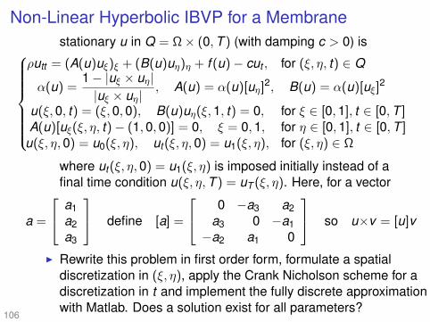
Non-Linear Hyperbolic IBVP for a Membranestationary u in Q = Ω× (0,T ) (with damping c > 0) is
ρutt = (A(u)uξ)ξ + (B(u)uη)η + f (u)− cut , for (ξ, η, t) ∈ Q
α(u) =1− |uξ × uη||uξ × uη|
, A(u) = α(u)[uη]2, B(u) = α(u)[uξ]2
u(ξ,0, t) = (ξ,0,0), B(u)uη(ξ,1, t) = 0, for ξ ∈ [0,1], t ∈ [0,T ]A(u)[uξ(ξ, η, t)− (1,0,0)] = 0, ξ = 0,1, for η ∈ [0,1], t ∈ [0,T ]
u(ξ, η,0) = u0(ξ, η), ut (ξ, η,0) = u1(ξ, η), for (ξ, η) ∈ Ω
where ut (ξ, η,0) = u1(ξ, η) is imposed initially instead of afinal time condition u(ξ, η,T ) = uT (ξ, η). Here, for a vector
a =
a1a2a3
define [a] =
0 −a3 a2a3 0 −a1−a2 a1 0
so u×v = [u]v
I Rewrite this problem in first order form, formulate a spatialdiscretization in (ξ, η), apply the Crank Nicholson scheme for adiscretization in t and implement the fully discrete approximationwith Matlab. Does a solution exist for all parameters?
106

Scalar Convection EquationI Finite Difference Methods for Conservation Laws will first
be investigated by considering the IVP for the scalarconvection equation,
ut (x , t)− αux (x , t) = 0, x ∈ R, t ∈ (0,T ]u(x ,0) = u0(x), x ∈ R
(30)where α > 0 is constant.
I The solution is given explicitly by the left traveling wave
u(x , t) = u0(x + αt), x ∈ R, t ≥ 0
so the IVP need not be solved numerically.I Yet the study of numerical methods for such a simple
problem will set the stage for the general theory.I The solution to (30) is approximated with forward spatial
differences by Uk (x) ≈ u(x , tk ) where tk = kτ , τ = T/K , and[Uk+1(x)−Uk (x)]/τ = α[Uk (x + h)−Uk (x)]/h, x ∈ R, 0≤k≤K−1
U0(x) = u0(x), x ∈ R107

Forward Difference SchemeI With the Courant Number r = ατ/h, the scheme becomes
Uk+1(x) = rUk (x + h) + (1− r)Uk (x), x ∈ R,0 ≤ k ≤ K − 1U0(x) = u0(x), x ∈ R
(31)I While a spatial grid xi = ih : i ∈ Z can be introduced, the
theory will be carried out using a continuous variable x .I Although a practical problem would involve a bounded
spatial domain and a boundary condition, the analysis ofthe IVP on an infinite domain can serve as a guide to thelocal behavior of a more realistic solution.
I A more detailed analysis is necessary when boundaryeffects would be significant.
I The analysis of (31) (stability, consistency, convergence)will be carried out in L2(R) with Hilbert space structure.
I The (extended) Fourier Transform will be used for f , f ∈ L2(R)
f (ξ) = (F f )(ξ) =1√2π
∫ +∞
−∞f (x)e−ıxξdx , ξ ∈ R (ı2 = −1)
108

Fourier Transformswith inverse formula, f (x) = (F−1 f )(x),
g(x) = (F−1g)(x) =1√2π
∫ +∞
−∞g(ξ)eıxξdx , x ∈ R
I By Parseval’s Identity,
(f ,g)L2 =
∫ +∞
−∞f (x)g∗(x)dx =
∫ +∞
−∞f (ξ)g∗(ξ)dξ = (f , g)L2
the Fourier and Inverse Fourier Transforms are isometricisomorphisms.
I For f ∈ L2(R) absolutely continuous with f (x)→ 0, |x | → ∞,it holds that
(F f ′)(ξ) = ıξ f (ξ).
I Under more general smoothness assumptions it holds that
(F f (n))(ξ) = (ıξ)n f (ξ).
I The translation operator (Taf )(x) = f (x + a) satisfies
(FTaf )(ξ) = eıξa f (ξ).109

Fourier TransformsI Under suitable regularity assumptions we take the Fourier
Transform of (30) to obtain
(Fux )(ξ, t) = ıξu(ξ, t), (Fut )(ξ, t) = ut (ξ, t)
and ut (ξ, t) = ıξαu(ξ, t), ξ ∈ R, t ∈ (0,T ]u(ξ,0) = u0(ξ), ξ ∈ R
I The solution to this ξ-parameterized ODE is
u(ξ, t) = eαıξt u0(ξ) = (FTαtu0)(ξ) or u(x , t) = u0(x+αt)
which implies the conservation ‖u(·, t)‖L2 = ‖u0‖L2 since
‖u(·, t)‖2L2 = ‖u(·, t)‖2L2 =
∫ +∞
−∞|eαıξt u0(ξ)|2dξ = ‖u0‖2L2 = ‖u0‖2L2
I We now consider convergence of the scheme (31). Takingthe Fourier Transform gives
Uk+1(ξ) = GUk (ξ) := Uk (ξ) + r [eıξhUk (ξ)− Uk (ξ)]110
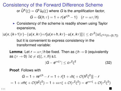
Consistency of the Forward Difference Schemeor Uk (ξ) = Gk u0(ξ) where G is the amplification factor,
G = G(h, τ) = 1 + r(eıξh − 1) (r = ατ/h)
I Consistency of the scheme is readily shown using Taylorexpansions,
|u(x , (k+1)τ)−u(x , kτ)+r [u(x+h, kτ)−u(x , kτ)]| ≤ cτ2‖u‖C2,0(R×[0,T ])
but it is convenient to express consistency in thetransformed variable:
Lemma: Let r = ατ/h be fixed. Then as ξh→ 0 (equivalentlyas ξτ → 0) ∃c 6= c(ξ, τ, h) s.t.
|G − eıαξτ | ≤ cτ2ξ2 (32)
Proof: Follows with
G = 1 + reıξh − r = 1 + r [1 + ıhξ +O(h2ξ2)]− r
= 1 + ırhξ +O(h2ξ2) = 1 + ıατξ +O(τ2ξ2) = eıατξ +O(τ2ξ2)
111

Stability of the Forward Difference SchemeI Furthermore, (with [1 + az +O(z2)]c = ec[az+O(z2)])
Gk = (G)tk/τ = [1+ıατξ+O(τ2ξ2)]tk/τ = eαıτξtk/τeO(τ2ξ2tk/τ)
= eαıξtk etkτξ2so Gk − eαıξkτ = eαıξtk [eO(tkτξ2) − 1]
I Then the pointwise convergence (r , tk fixed) follows:
limτ→0
[Uk (ξ)− u(ξ, tk )] = limτ→0
[Gk − eαıξkτ ]u0(ξ) = 0.
I However, pointwise convergence does not implyconvergence in L2(R). It must yet be shown that
‖Uk − u(·, tk )‖L2 = ‖Uk − u(·, tk )‖L2 → 0, τ → 0for which the following stability is required.
Lemma: Let u0 ∈ L2(R) and suppose r ∈ (0,1]. Then
‖Uk‖L2 ≤ ‖u0‖L2 , ∀k ≥ 0.
Proof: For r ∈ (0,1], |G| ≤ 1 follows from
|1 + reıξh − r | = |1− r + reıξh| ≤ |1− r |+ |r | = 1− r + r = 1.112

Stability of the Forward Difference SchemeFrom Uk (ξ) = Gk u0(ξ) it follows
|Uk (ξ)| = |G|k |u0(ξ)| ≤ |u0(ξ)|, ∀ξ ∈ Ror‖Uk‖2L2 = ‖Uk‖2L2 =
∫ +∞
−∞|Uk (ξ)|2dξ ≤
∫ +∞
−∞|u0(ξ)|2dξ = ‖u0‖2L2
I The condition |G| ≤ 1 is the Von Neumann stabilitycondition.
I The condition r ∈ (0,1] is seen above to be sufficient forstability. Yet it is also necessary:
Exercise: Construct an example for which the scheme (31)gives ‖Uk‖L2 →∞ as k →∞ for fixed tk = kτ and fixedr = ατ/h > 1.
I For convergence we introduce the following functionspaces (with minimal background).
Def: The Sobolev Space Hm(R) consists of those functionswhose derivatives up to order m are in L2(R).113

Sobolev SpacesI The Sobolev spaces have the Hilbert space structure with
the scalar product,
(u, v)Hm =m∑
l=0
∫ +∞
−∞u(l)(x)∗v (l)(x)dx
I By Parseval’s Identity and the derivative property
(u, v)Hm =m∑
l=0
∫ +∞
−∞[(ıξ)l u(ξ)]∗[(ıξ)l v(ξ)]dξ
I The norm on Hm(R) is then given by
‖u‖Hm =
[m∑
l=0
∫ +∞
−∞|u(l)(x)|2dx
] 12
=
[m∑
l=0
∫ +∞
−∞|ξ|2l |u(ξ)|2dξ
] 12
Theorem: Let u0 ∈ H2(R). Let r = ατ/h ∈ (0,1] be fixed. Then∃c 6= c(τ,h) s.t. for τ = T/K ,
max0≤k≤K
‖Uk − u(·, tk )‖L2 ≤ cτ‖u0‖H2114

Convergence of the Forward Difference SchemeProof: Using u(ξ, t) = eαıξt u0(ξ) and Uk (ξ) = Gk u0(ξ) gives
‖Uk−u(·, tk )‖2L2 = ‖Uk−u(·, tk )‖2L2 =
∫ +∞
−∞|u0(ξ)|2|Gk−eıαξkτ |2dξ
and this integral I is now partitioned as I = I1 + I2 with I1 takenover the set ξ : |ξ| ≥ γ/h and I2 over the set ξ : |ξ| < γ/h,where γ is to be determined. First consider I1. Note from|G| ≤ 1 that
|Gk − eıαξkτ |2 ≤ (|G|k + |eıαξkτ |)2 ≤ 4and hence
I1 ≤ 4∫|ξ|≥γ/h
|u0(ξ)|2dξ ≤ 4h2
γ2
∫|ξ|≥γ/h
|ξ|2|u0(ξ)|2dξ
=4α2τ2
r2γ2
∫|ξ|≥γ/h
|ξ|2|u0(ξ)|2dξ ≤ cτ2‖u′0‖2L2 ≤ cτ2‖u0‖2H2 .
Now consider I2. Let γ > 0 be chosen so that the consistencyestimate (32) holds for |hξ| < γ. Also note that for |a|, |b| ≤ 1,
|ak − bk | = |(a− b)∑k−1
m=0 ak−mbm| ≤ k |a− b|.115

Backward Difference SchemeHence for |hξ| < γ, (32) gives
|Gk − eıαξτk | ≤ k |G − eıαξτ | ≤ ckτ2ξ2 ≤ cT τξ2
Hence,I2 ≤ cτ2
∫|hξ|<γ
|u0(ξ)|2|ξ|4dξ ≤ cτ2‖u0‖2H2
I For r = 1 the scheme (31) is exact. (verify!)I For the IVP (30) with −α replaced by +α (again withα > 0) the solution is given by the right traveling waveu(x , t) = u0(x − αt) and is approximated with backwardspatial differences by Uk (x) ≈ u(x , tk ) where
[Uk+1(x)−Uk (x)]/τ = α[Uk (x)−Uk (x − h)]/h, x ∈ R, 0≤k≤K−1U0(x) = u0(x), x ∈ R
I Exercise: Find the amplification factor G for the backwarddifference scheme and show that |G| ≤ 1 holds iff r ∈ (0,1].Prove convergence of the scheme and determine the orderof convergence.
116

Lax Wendroff SchemeI Exercise: For the solution to ut + αux = 0 (with arbitrary
sign(α)), the Lax Wendroff scheme
Uk+1(x)− Uk (x)
τ= −αUk (x + h)− Uk (x − h)
2h
+α2τ
2Uk (x + h)− 2Uk (x) + Uk (x − h)
h2
x ∈ R, 0 ≤ k ≤ K − 1U0(x) = u0(x), x ∈ R
can be seen as a discretization of ut + αux = εuxxcontaining the artificial or pseudo-viscosity term εuxx withε = α2τ/2. Find the amplification factor G for the LaxWendroff scheme and show that |G| ≤ 1 holds iff |r | ≤ 1.Prove that the scheme converges with the order,
max0≤k≤K
‖Uk − u(·, tk )‖L2 ≤ cτ2‖u0‖H3
I Find the artificial viscosity term for the forward and thebackward difference schemes and observe the effect ofsign(α) for each.117

Linear Hyperbolic SystemsI Now for A ∈ Rm consider the IVP (Cauchy Problem),
ut + Aux = 0, x ∈ R, t > 0u = u0, x ∈ R, t = 0
(33)
I With the spatial grid xi = ih, h > 0, i ∈ Z, and the temporalgrid tk = kτ , τ > 0, k ∈ N0, let Uk
i denote anapproximation of the cell average,
uki =
1h
∫ xi+ 1
2
xi− 1
2
u(x , tk )dx
and define the piecewise constant function
Uτ (x , t) = Uki , (x , t) ∈ [xi− 1
2, xi+ 1
2)× [tk , tk+1).
I The ratio τ/h is assumed to be a fixed constant.I In practice, (33) is solved on a finite spatial domain, e.g.,
x ∈ (0,1), with, e.g., periodic boundary conditions,
u(0, t) = u(1, t), t ≥ 0118

Periodic and Inflow Boundary Conditionsor inflow boundary conditions, (figure forthcoming)
vj(0, t) = lj(t), λj > 0vj(1, t) = rj(t), λj < 0
t ≥ 0
where SAS−1 = Λ = diagλjmj=1, vj = v = Su and
vt + Λvx = S(ut + Aux ) = 0.
I An apparently natural discretization for (33) is
Uk+1i − Uk
iτ
+ AUk
i+1 − Uki−1
2h= 0
but this explicit Euler method is unstable. (verify!)I On the other hand, the implicit Euler method
Uk+1i − Uk
iτ
+ AUk+1
i+1 − Uk+1i−1
2h= 0
is stable but involves an unnatural and expensive couplingamong all numerical values at time tk+1.
119

Upwinding and Other Single-Step SchemesI Other methods considered earlier are: the forward
difference scheme, the backward difference scheme andthe Lax Wendroff scheme.
I Other well-known methods include the Lax Friedrichs scheme,Uk+1
i − (Uki+1 + Uk
i−1)/2τ
+ AUk
i+1 − Uki−1
2h= 0
and the Leapfrog scheme (figure forthcoming)
Uk+1i − Uk−1
i2τ
+ AUk
i+1 − Uki−1
2h= 0
but, while all other previously mentioned methods are single-step methods, the Leapfrog scheme is a two-step method.
I The upwind method is given by
Uk+1i − Uk
iτ
+ A+Uk
i − Uki−1
h+ A−
Uki+1 − Uk
i
h= 0
where A+ = SΛ+S−1, A− = SΛ−S−1
and Λ+ = maxΛ,0, Λ− = minΛ,0.120

Upwinding and Other Single-Step SchemesExercise:
I For Ω = (0,1) write the IBVPvtt = ω2vxx , (x , t) ∈ Ω× (0,∞)
v(0, t) = v(1, t), vx (0, t) = vx (1, t), t ∈ (0,∞)v(x ,0) = v0(x), vt (x ,0) = v1(x), x ∈ Ω
as a linear hyperbolic system ut + Aux = 0 with periodicboundary conditions and with appropriate initial conditions.
I Choose smooth data v0(x) = sin(2kπx), k ∈ N, and thenrough data v0(x) = (1
4 < x < 34), and then choose v1 so
that there are waves traveling (a) only to the right, (b) onlyto the left or (c) mirrored in both directions.
I Implement the single-step schemes above and estimatethe respective convergence rates. Report on apparentamplitude (dissipation) and phase (dispersion) errors.
I Write new boundary conditions so that left and right travelingwaves are purely absorbed at the left and right boundariesrespectively. Implement the upwind scheme for this problem.121

Consistency of Single-Step SchemesI All the one-step methods above can be written in the form
Uk+1i = Hτ (Uk ; i) or Uτ (x , t + τ) = Hτ (Uτ (·, t); x)
I Although the L2(R) norm was useful earlier in the contextof Fourier analysis, we will now use the L1(R) norm,
‖u‖L1 =
∫ +∞
−∞|u(x)|dx , ‖Uτ (·, tk )‖L1 = h
∑i
|Uki |
I A method is called consistent if for sufficiently smooth u
Lτ (x , t) = [u(x , t + τ)− Hτ (u(·, t); x)]/τ
satisfies ‖Lτ (·, t)‖L1 → 0, τ → 0.I For the Lax Friedrichs method, Taylor expansions give
Lτ (x , t) = [u(x , t + τ)− (u(x − h, t) + u(x + h, t))/2]/τ+A[u(x + h, t)− u(x − h, t)]/(2h)
= ut + Aux + 12 [τutt − (h2/τ)uxx ] +O(h2)
122

Stability of Single-Step Schemessince τ/h is constant, so with ut + Aux = 0,
Lτ (x , t) = 12τ [A2 − (h/τ)2I]uxx +O(τ2)
and given that u0 has compact support, so does uxx and
‖Lτ (·, t)‖L1 ≤ cτ
I A method is called stable if ∀T , ∃c, τ0 > 0 such that
‖Hkτ ‖L1 ≤ c, ∀k , τ with kτ ≤ T , and τ < τ0.
I For the Lax Friedrichs method with A = α > 0 and ατ/h ≤ 1,
‖Uk+1‖L1 = h∑
i |Uk+1i |
≤ h2∑
i |(1− ατ/h)Uki+1|+
h2∑
i |(1 + ατ/h)Uki−1|
= 12(1− ατ/h)‖Uk‖L1 + 1
2(1 + ατ/h)‖Uk‖L1 = ‖Uk‖L1
Lax Equivalence Theorem: A consistent, linear method isconvergent if and only if it is stable.
Proof: (sufficiency) Set Eτ (x , t) = Uτ (x , t)− u(x , t). With the123

Lax Equivalence Theoreminitial values consistently approximated, we have that‖Eτ (·,0)‖L1 → 0 as τ → 0. Also
Eτ (x , t + τ) = Hτ (Eτ (·, t); x)− τLτ (x , t)satisfies
Eτ (x , tk ) = Hkτ (Eτ (·,0); x)− τ
k∑l=1
Hk−lτ (Lτ (·, tl−1); x)
and hence with ‖Hkτ ‖L1 ≤ c,
‖Eτ (·, tk )‖L1 ≤ ‖Hkτ ‖L1‖Eτ (·,0)‖L1 + τ
k∑l=1
‖Hk−lτ ‖L1‖Lτ (·, tl−1)‖L1
≤ c[‖Eτ (·,0)‖L1 + T max
1≤l≤k‖Lτ (·, tl−1)‖L1
]→ 0
as τ → 0.I Exercise: Show that the Lax Friedrichs scheme converges
if the CFL condition (Courant, Friedrichs, Lewy) is satisfied:
|λjτ/h| ≤ 1, ∀j = 1, . . . ,m.
I Exercise: Show that the backward difference schemeconverges if (and only if) 0 ≤ λjτ/h ≤ 1.124

Computing Discontinuous SolutionsI While wave equations are often given in differential form,
the underlying principle involves conservation of integratedquantities, which are not necessarily pointwise smooth.
I Physical waves often involve shocks, i.e., discontinuities.I For a sufficiently smooth solution to (30), the Lax
Friedrichs scheme converges as O(τ), and the LaxWendroff scheme converges as O(τ2).
I When (30) is solved (weakly) by a traveling shock wave,I first-order schemes, e.g., Lax Friedrichs, typically give
smearing around discontinuities (converging as O(τ12 )), and
I second-order schemes, e.g., Lax Wendroff, typically giveoscillations around discontinuities (converging as O(τ
23 )).
(figure forthcoming)I To explain this behavior, a scheme can be seen to provide
a higher order approximation of the solution to a so-calledmodified equation, which depends upon discretizationparameters.
125

Modified EquationsI For example, it was shown above for Lax Friedrichs that
Lτ (x , t) = ut + Aux + 12τ [A2 − (h/τ)2I]uxx +O(τ2)
and hence the scheme can be viewed as providing a O(τ2)approximation of the solution to the dissipation equation
ut + Aux = Duxx , D =h2
2τ
[I − τ2
h2 A2]
I For |τλj/h| < 1, the matrix D and the term uxx lead toforward diffusion, which smears out shocks. Backwarddiffusion results from |τλj/h| > 1, which is unstable.
I Exercise: Determine the modified equation for the explicitEuler method
Uk+1i − Uk
iτ
+ AUk
i+1 − Uki−1
2h= 0
and use this to explain why the method is unstable for all τ/h.126

Dissipation and DispersionI The modified equation for the Lax Wendroff method is the
dispersion equation (verify!)
ut + Aux = Duxxx , D =h2
6A[τ2
h2 A2 − I]
I For the case A = α > 0 and D = µ, taking the FourierTransform of the dispersion equation gives
ut (ξ, t) + ıξαu(ξ, t) = µ(ıξ)3u(ξ, t), u(ξ,0) = u0(ξ)
which is solved by
u(ξ, t) = e−ıc(ξ)t u0(ξ), c(ξ) = αξ + µξ3
I Considering each frequency component separately, setu0(x) = eıκx to obtain u(ξ) =
√2πδ(ξ − κ) and the
traveling wave solution e−ıc(κ)tF−1[√
2πδ(ξ − κ)] or
u(x , t) = eı(κx−c(κ)t) = eıκ(x−cp(κ)t), cp(κ) = c(κ)/κ = α+ µκ2
with phase velocity cp(κ), the speed at which wave peakstravel, depending upon the wave number κ excited in u0.127

Phase and Group VelocitiesI A step function, such as u0(x) = sign(x), has a broad
Fourier spectrum, u0(ξ) =√
2/π/(ıξ).I For such broad spectrum data, the wave number κ is
mainly visible near x = cg(κ)t instead of x = αt , wherecg(κ) = c′(κ)
is the group velocity.I For Lax Wendroff, cg(κ) = α + 3µκ2, so higher frequency
components are dispersed more.I Numerical errors due to dissipation and dispersion can
also be quantified with the amplification factor:I Let Ge(κ, τ) = ρe(κ, τ)eıφe(κ,τ) (ρe, φe ∈ R) denote the singleτ step amplification factor for an exact solution with spatialwave number κ.
I Let Gc(κ, τ) = ρc(κ, τ)eıφc (κ, τ) (ρc, φc ∈ R) denote thecorresponding amplification factor for the computedsolution.
Relative dissipation and dispersion errors are respectively
ρc(κ, τ)/ρe(κ, τ) and |φc(κ, τ)/φe(κ, τ)|.128

Relative Dissipation and Dispersion ErrorsI Example: With wave number κ in u0(x) = eıκx , (30) is
solved exactly by ue(x , t) = eı(κx+ωet) iff ωe = −ακ, soGe(κ, τ) = e−ıακτ and u(x , t + τ) = Ge(κ, τ)u(x , t).
I For the upwind scheme Uk+1i = (1− |r |)Uk
i + |r |Uki−σ(a)
with r = ατ/h, σ(α) = sign(α) and Uki = eı(κxi +ωetk ),
Gc(κ, τ) = (1− |r |) + |r |e−ı|α|κτ/r and Uk+1i = Gc(κ, τ)Uk
i .I In Ge(κ, τ) = eıωeτ and Gc(κ, τ) = eıωcτ , ωe(κ, τ) and ωc(κ, τ)
are the so-called exact and computed dispersion relations.I The relative dissipation error is
ρc(κ, τ)/ρe(κ, τ) =[1− 4|r |(1− |r |) sin2(ακτ/(2r))
] 12
implying some dissipation unless |r | = 1.I The relative dispersion error is
|φc(κ, τ)/φe(κ, τ)| = tan−1[
|r | sin(κατ/r)
(1− |r |+ |r | cos(κατ/r))
] /(aκτ)
implying no dissipation error for |r | = 12 ,1, while there is a
phase lag for |r | < 12 and a phase advance for |r | > 1
2 .tan θ/2 =
sin θ1+cos θ
I Exercise: Repeat for Lax Friedrichs and Lax Wendroff.129

Burger’s EquationI A scalar conservation equation often used to model
aspects of fluid flow is Burger’s Equationut + 1
2(u2)x = 0which is deduced from the weak (integral) form of solution,∫ x2
x1
[u(x , t2)−u(x , t1)]dt+∫ t2
t1[f (x2, t)−f (x1, t)]dt = 0, ∀[x1, x2]×[t1, t2]
with flux f (u) = u2/2 of the conserved quantity u.I When Burger’s equation is written in the quasilinear form
ut + uux = 0, u(x ,0) = u0(x)
the coefficient u can be viewed as the wave speed (cf. α in(30)), and an apparently natural upwind scheme is given by
(Uk+1i − Uk+1
i )/τ + Uki (Uk
i − Uki−1)/h = 0
assuming that Uki ≥ 0. Yet for u0(x) = (x < 0), we obtain
Uτ (x)→ u0(x), τ → 0, which is not a weak solution.I Exercise: Verify these claims.
130

Conservative Methods for Nonlinear ConvectionI To avoid convergence to non-solutions, it is required that
numerical methods for solving ut + f (u)x = 0 can beexpressed in conservative form,
(Uk+1i −Uk
i )/τ+[F (Uk ; i)−F (Uk ; i−1)]/h = 0, F (Uk ; i)=F (Ui+jqj=−p)
where F is the numerical flux function.I The simplest and most frequently used case is (p = 0, q = 1)
(Uk+1i − Uk
i )/τ + [F (Uki ,U
ki+1)− F (Uk
i−1,Uki )]/h = 0
I Considering the weak form of the conservation equation on[xi− 1
2, xi+ 1
2]× [tk , tk+1], conservative form implies naturally that
F (Uki ,U
ki+1) ≈ 1
τ
∫ tk+1
tkf (u(xi+ 1
2, t))dt
I An approach to upwinding for nonlinear fluxes is to use
F (U,V ) =
f (U), [f (U)− f (V )]/(U − V ) ≥ 0f (V ), [f (U)− f (V )]/(U − V ) < 0
with generlizations for systems to be addressed later.131

Consistency for Conservative MethodsI The Lax Friedrichs scheme for nonlinear systems is
[Uk+1i − 1
2(Uki−1 + Uk
i+1)]/τ + [f (Uki+1)− f (Uk
i−1)]/(2h) = 0
with the corresponding numerical flux function
F (Uki ,U
ki+1) =
h2τ
[Uki − Uk
i+1] +12
[f (Uki ) + f (Uk
i+1)]
I A conservative scheme is said to be consistent if thenumerical flux function is Lipschitz continuous and satisfiesF (u,u, . . . ,u) = f (u). (So f is necessarily Lipschitz.)
I Exercise: Show that the upwind and Lax Friedrichs schemesare consistent. Also discuss a nonlinear Lax Wendroff scheme.
Theorem: (Lax Wendroff) Choose grid parameters τl → 0 andhl → 0 as l →∞. Let Ul(x , t) be given on the l-th grid by aconservative scheme which is consistent with ut + f (u)x = 0.Suppose Ul converges with bounded variation in L1
loc to u, i.e.,∀Ω = (x1, x2)× (t1, t2) ⊂ R× [0,∞), ‖Ul − u‖L1(Ω) → 0, l →∞,and ∀T > 0, ∃c > 0 such that TV(Ul(·, t)) ≤ c, ∀t ∈ [0,T ], ∀l .Then u is a weak solution to the conservation equation.132

Lax Wendroff TheoremProof: A weak solution u can characterized equivalently by∫ ∞
0
∫ +∞
−∞[φtu+φx f (u)]dxdt =−
∫ +∞
−∞φ(x ,0)u0(x ,0)dx , ∀φ ∈ C1
0(R×[0,∞))
For such a φ multiply the scheme by φ(xi , tk ) to obtain
φ(xi , tk )[Uk+1i − Uk
i ]/τ + φ(xi , tk )[F (Uk ; i)− F (Uk ; i − 1)]/h = 0
and sum over all i and k ≥ 0,∞∑
k=0
+∞∑i=−∞
φ(xi , tk )Uk+1
i − Uki
τ+∞∑
k=0
+∞∑i=−∞
φ(xi , tk )F (Uk ; i)− F (Uk ; i −1)
h=0.
After summation by parts, i.e.,
m∑i=1
ai(bi − bi−1) = ambm − a1b0 −m−1∑i=1
(ai+1 − ai)bi
we obtain the following, using the compact support of φ, i.e.,φ(xi , tk ) = 0 for |i | or k sufficiently large,133

Lax Wendroff Theorem
−+∞∑
i=−∞φ(xi ,0)U0
i /τ −∞∑
k=1
+∞∑i=−∞
φ(xi , tk )− φ(xi , tk−1)
τUk
i
−∞∑
k=0
+∞∑i=−∞
φ(xi+1, tk )− φ(xi , tn)
hF (Uk ; i) = 0
where each sum is finite, owing to the compact support of φ.Multiplying by h and rearranging gives
hτ∞∑
k=1
+∞∑i=−∞
(φ(xi , tk )− φ(xi , tk−1)
τ
)Uk
i
+hτ∞∑
k=0
+∞∑i=−∞
(φ(xi+1, tk )− φ(xi , tk )
τ
)F (Uk ; i)
= −h+∞∑
i=−∞φ(xi ,0)U0
i .
Due to the convergence in L1loc of U and the smoothness of φ,
the first and last terms converge respectively to134

Lax Wendroff Theorem∫∞0
∫ +∞−∞ φt (x , t)u(x , t)dxdt
and−∫ +∞−∞ φt (x , t)u(x ,0)dx
as l →∞. For the remaining term in the last equation note
|F (Uk ; i)− f (Uki )| ≤ L max
−p≤j≤q|Uk
i−j − Uki | → 0, a.e. l →∞
where the first inequality follows from consistency and theconvergence follows from bounded variation. Thus, F (Uk ; i)above can be approximated by f (Uk
i ) with errors that vanishuniformly a.e. Similarly, due to Lipschitz continuity of f ,
|f (Uki )− f (uk
i )| ≤ L|Uki − uk
i |
a difference which converges to 0 in L1loc. Thus, F (Uk ; i) above
can actually be approximated by f (uki ) with errors that vanish
uniformly. The resulting term converges to∫∞0
∫ +∞−∞ φx (x , t)f (u(x , t))dxdt
as l →∞.135

Vanishing Viscosity SolutionsI Weak solutions to conservation equations ut + f (u)x = 0
are typically not unique.I A weak solution is regarded as correct when it corresponds
to a vanishing viscosity solution, i.e., limε→0 uε where
uεt + f (uε)x = εuxx
I A vanishing viscosity solution can be characterized moreconveniently as an entropy solution, one which is eithersmooth or else exhibits shocks with the property thatcharacteristics never emerge from but rather always runinto space-time discontinuities.
I Examples: Entropy (vanishing viscosity) solutions toBurger’s equation are given by
u(x , t) = −sign(x), u0(x) = −sign(x) (shock)and (figure forthcoming)
u(x , t) =
−1, x ≤ −tx/t , −t ≤ x ≤ t+1, t ≤ x
u0(x) = sign(x) (rarefaction)
136

Entropy Solutions to Conservation Equations
I In the second case above, a weak solution which is not anentropy solution is given by
u(x , t) = sign(x), u0(x) = sign(x) (shock)
I Exercise: Verify these claims.I Exercise: For initial data U0
i = (i > 0)− (i ≤ 0), show thatthe nonlinear upwind scheme converges to the entropyviolating shock above.
I Exercise: For initial data given by cell averages ofu0(x) = sign(x), show that with h = 2τ the nonlinearupwind scheme
I converges to the correct rarefaction wave for τl = 1/(2l) asl →∞,
I converges to the entropy violating shock for τl = 1/(2l + 1)as l →∞,
I diverges for τl = 1/l as l →∞.
137

Roe’s Approximate Riemann SolverI A Riemann Solver for a conservation equation
ut + f (u)x = 0 is one in which a weak solution isapproximated in the time interval [tk , tk+1] using the exactsolution for piecewise constant data, (Riemann problems)
u(x , tk ) = Uki , x ∈ (xi− 1
2, xi+ 1
2)
I The solution can be computed exactly over a short timeinterval, and then cell averages may be recomputed.
I This is the essence of Godunov’s Method, but exactRiemann solvers can be expensive.
I The idea of Roe’s Approximate Riemann Solver is to solvea constant coefficient linear hyperbolic system at every cellinterface,
ut + A(ul,ur)ux = 0
where the matrix A(ul,ur) depends upon left and rightstates ul and ur at the interface.
138

Roe’s Approximate Riemann SolverI Roe requires the following conditions on A(ul,ur):
1. A(ul,ur)(ul − ur) = f (ul)− f (ur),2. A(ul,ur) is diagonalizable with real eigenvalues,3. A(ul,ur)→ f ′(u), ul,ur → u.
I The associated numerical flux function is given by
F (ul,ur) = [f (ur) + f (ul)]/2− |A(ul,ur)|(ur − ul)/2
where A+ = SΛ+S−1, A− = SΛ−S−1,
|A| = A+ − A− = S|Λ|S−1, |Λ| = Λ+ − Λ−
and Λ+ = maxΛ,0, Λ− = minΛ,0.I In some cases one may take A(ul,ur) = f ′(uave), where uave
is a certain average of ul and ur, difficult to implement inpractice. Yet, a Roe matrix can be shown to exist for certainapplications, e.g., scalar equations and Euler equations.
I For a scalar conservation equation, ut + f (u)x = 0,A(ul,ul) = α(ul,ul) is given uniquely by
α(ul,ul) = [f (ur)− f (ul)]/[ur − ul]139

Code to Solve Burger’s EquationI Matlab code to solve Burger’s Equation with Roe’s scheme:
N1 = N+1; N2 = N+2; dx = 1/N1;dt = dx/10; K = round(1/dt); T = K*dt; r = dt/dx;x = linspace(-1,+1,N2); u = 0.5*sign(x); uv = u;for k=1:K
f = u.ˆ2/2;ul = u(1:N1); fl = f(1:N1);ur = u(2:N2); fr = f(2:N2);df = fr-fl; du = ur-ul;a = df.*(du ˜= 0)./(du + (du == 0));F = (fl + fr)/2 - abs(a).*du/2;dF = [0,F(2:N1)-F(1:N),0];u = u - r*dF;u(1) = u(1) - r*(a(1) < 0)*df(1);u(N2) = u(N2) - r*(a(N1) > 0)*df(N1);plot(x,u); uv = [uv;u];
endcontour(uv,’Fill’,’on’);140

Roe Matrix for Isothermal FlowI The Euler equations for inviscid flow in one spatial
dimension (e.g., in a pipe) are given by:mass conservation: ρt + (ρv)x = 0
momentum conservation: (ρv)t + (ρv2 + p)x = 0energy conservation: Et + (v(E + p))x = 0
where the pressure is determined by an equation of statep = p(ρ, v ,E).
I If the temperature is constant, the energy E can be determinedfrom the density ρ and the velocity v without solving the energyconservation equation. The equation of state reduces top = a2ρ where a is the sound speed. The Euler equationsreduce to
ut + f (u)x = 0, u =
[ρρv
], f (u) =
[ρv
ρv2 + a2ρ
]I Exercise: Use the following Roe matrix to solve this system.
A(ul,ur) =
[0 1
a2 − v2 2v
], v =
ρ1/2l vl + ρ
1/2r vr
ρ1/2l + ρ
1/2r141

Convection Diffusion EquationI Previous techniques for conservation equations are now
applied to solve the convection diffusion PDE in Ω = (0,1)2,∂tu +∇ · (αu) = ∇ · (κ∇u) + φ in Ω× (0,T ]
u = g1, on ∂Ω1 × [0,T ]∂nu = g2, on ∂Ω2 × [0,T ]
u = u0, in Ω× 0
where ∂Ω = ∂Ω1 ∪ ∂Ω2, α : Ω→ R2 and κ : Ω→ R+.I For compatibility it must be that u0|∂Ω1 = g1 and∂nu0|∂Ω2 = g2 hold.
I Without loss of generality we may assume that g2 = 0.Otherwise, we could shift this boundary condition to theinterior as follows:
I Define a sufficiently smooth function v satisfying∂nv |∂Ω2 = g2, e.g., v = u0 if g2 is independent of t .
I Solve the convection diffusion PDE for w = u − v replacing(a) φ with φ+∇ · (κ∇v)−∇ · (αv)− ∂tv , (b) g1 with g1 − vand (c) u0 with u0 − v .
I Take u = w + v to solve the original problem.142

Convection Diffusion EquationI For N ∈ N and h = 1/(N + 1) set
Ωh = (x , y) : x = ih, y = jh,0 ≤ i , j ≤ N + 1
and for K ∈ N and τ = T/K set tk = kτ , 0 ≤ k ≤ K .I The exact solution uk
ij = u(xi , yj , tk ) to the PDE isapproximated with Uk
ij ≈ ukij written as Uk
h = Ukij
N+1i,j=0.
I The diffusivity is evaluated at midpoints (x + 12 ih, y + 1
2 jh),|i |+ |j | = 1, between grid points (x , y) ∈ Ωh,
κh,x =κ(xi + 1
2 ih, yj)N,N+1
i=0,j=0 , κh,y =κ(xi , yj + 1
2 jh)N+1,N
i=0,j=0
I Let D(V ) denote a diagonal matrix with the values of thevector V along the diagonal.
I Using Dh,x and Dh,y for Neumann boundary conditionsfrom 76 , the diffusion term is approximated by
−∇ · (κ∇u) ≈ Ah,κU, Ah,κ = D>h,xD(κh,x )Dh,x + D>h,yD(κh,y )Dh,y143

Convection Diffusion Equation
I For α = (α1, α2) set f (u) = α1u and g(u) = α2u orαu = (f (u),g(u)). The convection is approximated usingupwinding, (ut + f (u)x + g(u)y )i,j ≈
Uk+1i,j − Uk
i,j
τ+
F ki+ 1
2 ,j− F k
i− 12 ,j
h+
Gki,j+ 1
2−Gk
i,j− 12
h
where the numerical flux functions for f and g are givenrespectively by
F ki+ 1
2 ,j=
f ki+1,j + f k
i,j
2−|ak
i+ 12 ,j|Uk
i+ 12 ,j− Uk
i− 12 ,j
2, ai+ 1
2 ,j=
f ki+1,j − f k
i,j
Uki+ 1
2 ,j− Uk
i− 12 ,j
Gki,j+ 1
2=
gki,j+1 + gk
i,j
2−|ak
i,j+ 12|Uk
i,j+ 12− Uk
i,j− 12
2, ai,j+ 1
2=
gki,j+1 − gk
i,j
Uki,j+ 1
2− Uk
i,j− 12
144

Convection Diffusion EquationI Define the numerical flux vectors
δF kh =
Fi+ 1
2 ,j− Fi− 1
2 ,j, 0 < i < N + 1
(a 12 ,j< 0)(f1,j − f0,j), i = 0
(aN+ 12 ,j> 0)(fN+1,j − fN,j), i = N + 1
δGkh =
Gi,j+ 1
2−Gi,j− 1
2, 0 < j < N + 1
(ai, 12< 0)(gi,1 − gi,0), j = 0
(ai,N+ 12> 0)(gi,N+1 − gi,N), j = N + 1
I Assume Ukh = gk
1 holds on ∂Ω1,h.I Let Uk+1
h be chosen to satisfy Uk+1h = gk+1
1 on ∂Ω1,h.I Define χh(x , y) = ((x , y) 6∈ ∂Ω1,h) as the characteristic
function for Ωh\∂Ω1,h.I Apply the semi-implicit scheme with r = τ/h,
[I+τD(χh)Ah,κ]Uk+1h = D(χh)[Uk
h−rδF kh−rδGk
h ]+D(1−χh)Uk+1h
I Note that Uk+1h = gk+1
1 necessarily holds on ∂Ω1,h.145

Code to Solve Convection Diffusion PDEN1 = N+1; N2 = N+2; N1N2 = N1*N2; N2N2 = N2*N2;dx = 1/N1; dt = dx/10; K = round(1/dt); T = K*dt;r = dt/dx; y = linspace(0,1,N2); x = y’; dy = dx;ax = 1.0e+0*ones(N2,N2); ay = 1.0e+0*ones(N2,N2);kx = 1.0e-2*ones(N1,N2); ky = 1.0e-2*ones(N2,N1);u = [ones(1,N2);zeros(N1,N2)]; u0 = u(:); U = u0;D0 = speye(N2); bcs = 1:N2:N2N2;D1 = spdiags(kron([-1,1],ones(N2,1)),[0,1],N1,N2);Dx = kron(D0,D1)/dx; Dy = kron(D1,D0)/dy;A = Dx’*spdiags(kx(:),0,N1N2,N1N2)*Dx ...
+ Dy’*spdiags(ky(:),0,N1N2,N1N2)*Dy; A(bcs,:)=0;for k=1:K
ul = u(1:N1,:); ur = u(2:N2,:); du = ur - ul;f = ax.*u;fl = f(1:N1,:); fr = f(2:N2,:); df = fr - fl;a = df.*(du ˜= 0)./(du + (du == 0));F = (fl + fr)/2 - abs(a).*du/2;
146

Code to Solve Convection Diffusion PDEdF = [(a(1,:)<0).*df(1,:); ...
F(2:N1,:)-F(1:N,:); ...(a(N1,:)>0).*df(N1,:)]; dF = dF(:);
ul = u(:,1:N1); ur = u(:,2:N2); du = ur - ul;g = ay.*u;gl = g(:,1:N1); gr = g(:,2:N2); dg = gr - gl;a = dg.*(du ˜= 0)./(du + (du == 0));G = (gl + gr)/2 - abs(a).*du/2;dG = [(a(:,1)<0).*dg(:,1), ...
G(:,2:N1)-G(:,1:N), ...(a(:,N1)>0).*dg(:,N1)]; dG = dG(:);
dF(bcs) = 0; dG(bcs) = 0; dU = U - r*dF - r*dG;U = (speye(N2N2) + dt*A) \ dU;u = reshape(U,N2,N2); surf(x,y,u);
end
Exercise: Implement convection as above and also with centraldifferences and compare.147

Function Spaces for Elliptic PDEsI Let Ω ⊂ Rn, n ∈ N, be open.I The Lebesgue Spaces Lp(Ω) are Banach spaces
consisting of (equivalence classes of) Lebesguemeasurable functions (differing at most on a set ofmeasure 0) with finite norm,
‖f‖Lp(Ω) =
(∫Ω|f (x)|pdx
) 1p
, 1 ≤ p <∞, ‖f‖L∞(Ω) = esssupx∈Ω
|f (x)|
I These satisfy Holder’s Inequality,
‖fg‖L1(Ω) ≤ ‖f‖Lp(Ω)‖g‖Lq(Ω), p−1 + q−1 = 1, p ≥ q.
So for bounded Ω it follows that Lp(Ω) → Lq(Ω), p ≥ q.I Also, L1
loc(Ω) = ∩K⊂⊂ΩL1(K ).I For p = 2, L2(Ω) is a Hilbert space with the scalar product,
(f ,g)L2(Ω) =
∫Ω
f (x)g(x)dx
and for p = q = 2, Holder’s Inequality gives theCauchy-Schwarz Inequality.
148

Lebesgue and Holder SpacesI The Holder Spaces Ck (Ω) are Banach spaces consisting of
functions whose partial derivatives ∂αu, |α| ≤ k , arecontinuous on Ω with finite norm,
‖u‖Ck (Ω) =∑|α|≤k
supx∈Ω|∂αu(x)|
I Ck0 (Ω) is the subspace of Ck (Ω) consisting of functions with
support Ku, Ku = x ∈ Ω : u(x) 6= 0, satisfying Ku ⊂⊂ Ω.I Ck (Ω) is the restriction to Ω of functions in Ck
0 (Rn).I Also C∞0 (Ω) = ∩k≥0Ck
0 (Ω).I A function u ∈ L1
loc(Ω) has an α-th weak derivativev ∈ L1
loc(Ω) in Ω, written v = ∂αu, if∫Ω
u(x)∂αφ(x)dx = (−1)|α|∫
Ωv(x)φ(x)dx , ∀φ ∈ Ck
0 (Ω)
I Example: u(x) = |x | has the weak derivativev(x) = sign(x) in Ω = (−1,+1), but v does not have aweak derivative in Ω.149

Weak Derivatives and Sobolev SpacesI The Sobolev Space W k ,p(Ω), k ∈ N0, 1 ≤ p ≤ ∞, are
Banach Spaces consisting of functions whose weakderivatives ∂αu, |α| ≤ k , are in Lp(Ω) with finite norm,
‖u‖W k,p(Ω) =
( ∑|α|≤k
‖∂αu‖pLp(Ω)
) 1p
, ‖u‖W k,∞(Ω) =∑|α|≤k
‖∂αu‖∞Lp(Ω)
I One also uses the semi-norms,
|u|W k,p(Ω) =
( ∑|α|=k
‖∂αu‖pLp(Ω)
) 1p
, |u|W k,∞(Ω) =∑|α|=k
‖∂αu‖∞Lp(Ω)
I An alternative definition of the Sobolev Space Hk ,p(Ω),k ∈ N0, 1 ≤ p <∞, is given by the completion of C∞(Ω)with respect to the W k ,p(Ω) norm above.
I Yet for ∂Ω sufficiently smooth, W k ,p(Ω) = Hk ,p(Ω) !I Here it will always be assumed that ∂Ω is Lipschitz
continuous, which is sufficient to insure that:I C∞(Ω) is dense (in Hk ,p(Ω) by definition and hence) in
W k ,p(Ω) for k ∈ N0, 1 ≤ p <∞.150

Sobolev EmbeddingsI For 1 ≤ p,q <∞ and Ω ⊂ Rn open and bounded with
Lipschitz ∂Ω, the following embeddings are continuous
W k ,p(Ω) →
Lq(Ω), p < n/k , p ≤ q ≤ np/(n − p)Lq(Ω), p = n/k , p ≤ q < np/(n − p)C0(Ω), p > n/k
I and the following embeddings are compact
W k ,p(Ω) →
Lq(Ω), p ≤ n/k , 1 ≤ q < (n − pk)/(np)C0(Ω), p > n/k
In particular, the embedding W k ,p(Ω) →W k−1,p(Ω) iscompact ∀k ∈ N, ∀p ∈ [1,∞].
I For Ωi ⊂ Rn, i = 0, . . . ,N, N ∈ N, open and bounded withLipschitz ∂Ωi such that Ωi ∩ Ωj = ∅, Ω = Ω0 = ∪N
i=1Ω, thefollowing holds ∀k ∈ N, ∀p ∈ [1,∞],
v ∈ Ck−1(Ω) : v |Ωi ∈ Ck (Ωi),1 ≤ i ≤ N ⊂W k ,p(Ω)
151

TracesI Let Ω ⊂ Rn be open and bounded with Lipschitz ∂Ω. Set
k ∈ N0, 1 ≤ p <∞, kp < n and 1 ≤ q ≤ (n− 1)p/(n− kp).Let T be a linear operator satisfying Tφ = φ|∂Ω forφ ∈ Ck (Ω).
I Then T has a unique extention to a bounded linear operatorT : W k ,p(Ω)→ Lq(∂Ω), and ∃c = c(p,Ω) > 0 such that
‖Tf‖Lq(∂Ω) ≤ c‖f‖W k,p(Ω), ∀f ∈W k ,p(Ω)
I If kp = n holds, then the estimate holds for any p ≤ q <∞.I Thus, one defines the subspace,
W k ,p0 (Ω) = f ∈W k ,p(Ω) : T∂αf = 0 ∈ Lq(∂Ω), |α| ≤ k − 1
or equivalently Hk ,p0 (Ω) (= W k ,p
0 (Ω)) as the completion ofC∞0 (Ω) with respect to the W k ,p(Ω) norm.
I Thus C∞0 (Ω) is dense in the subspace.I For the following let Pk denote the set of polynomials of
degree at most k .152

Poincare’s InequalityTheorem (Poincare): Let Ω ⊂ Rn be open and bounded withLipschitz ∂Ω. Let k ∈ N and 1 ≤ p <∞. Then ∃c = c(Ω) > 0such that
‖f‖W k,p(Ω) ≤ c|f |W k,p(Ω), ∀f ∈W k ,p0 (Ω)
Proof: Assume for the sake of contradiction, ∃fi ⊂W k ,p0 (Ω)
such that |fi |W k,p(Ω)/‖fi‖W k,p(Ω)i→∞−→ 0. Define fi = fi/‖fi‖W k,p(Ω)
so that ‖fi‖W k,p(Ω)∀i= 1 while |fi |W k,p(Ω)
i→∞−→ 0. Since fi isbounded in W k ,p(Ω) and W k ,p(Ω) is compactly embedded inW k−1,p(Ω), there is a subsequence fi ′ which convergesstrongly in W k−1,p
0 (Ω) to a limit f ∗ ∈W k−1,p0 (Ω). Yet since
|fi ′ |W k,p(Ω)i ′→∞−→ 0, the subsequence fi ′ is actually Cauchy in
W k ,p0 (Ω), meaning that f ∗ ∈W k ,p
0 (Ω). Since|f ∗|W k,p(Ω) = limi ′→∞ |fi ′ |W k,p(Ω) = 0, it must be that ∂αf ∗ = 0, ∀αwith |α| = k , or that f ∗ ∈ Pk−1. Yet since T∂αf ∗ = 0 on ∂Ω for|α| ≤ k − 1, it must be that f ∗ = 0. However, this contradicts‖f ∗‖W k,p(Ω) = limi ′→∞ ‖fi ′‖W k,p(Ω) = 1.
153

Poincare’s InequalityI One writes Hk (Ω) = W k ,2(Ω), Hk
0 (Ω) = W k ,20 (Ω), k ∈ N.
These are equipped respectively with the scalar products,(f ,g)Hk (Ω) =
∑|α|≤k
(∂αf , ∂αg)L2(Ω), (f ,g)Hk0 (Ω) =
∑|α|=k
(∂αf , ∂αg)L2(Ω)
and, based upon Poincare’s inequality, the associated norms
‖f‖Hk (Ω) = (f , f )12Hk (Ω)
, ‖f‖Hk0 (Ω) = |f |Hk (Ω) = (f , f )
12Hk
0 (Ω)
I Exercise: Show that the scalar product(∇u,∇v)L2(Ω)n + 〈u, v〉L2(∂Ω) induces a norm on H1(Ω).
I The dual of Hk0 (Ω) (i.e., the bounded linear functionals on
Hk0 (Ω)) is denoted by H−k (Ω) = (Hk
0 (Ω))∗ equipped withthe (operator) norm,
‖f‖H−k (Ω) = supφ∈Hk
0 (Ω),φ 6=0
f (φ)
‖φ‖Hk0 (Ω)
where f (φ) = (f , φ)H−k (Ω),Hk0 (Ω) is the duality pairing.
I Note (Hk0 (Ω))∗ = span∂αTf : |α| ≤ k ,T ∈ C∞0 (Ω)∗, f ∈ L2(Ω),
where f is an actual function. Not so for (Hk (Ω))∗.154

Weak Formulation of Elliptic BVPsI The strong form (implicitly requiring strong regularity) of a
typical elliptic PDE isLu = f , in ΩBu = g, on ∂Ω
(34)
where Ω ⊂ Rn is open and bounded with Lipschitz ∂Ω and
Lu(x) = −∇ · [A(x)∇u(x)] + c>(x)∇u(x) + r(x)u(x)
for given A = aijni,j=1, c = bini=1, r , f and g, sufficientlysmooth functions on Ω.
I Also, typical boundary conditions are given by
Bu(x) = σ1(x)n>A(x)∇u(x) + σ0(x)u(x)
for given σ1 and σ0, sufficiently smooth functions on ∂Ω.I Here σ1 = 0 gives pure Dirichlet BCs, σ0 = 0 gives pure
Neumann BCs, and σ1, σ0 > 0 gives Robin BCs.155

Weak Formulation of Elliptic BVPsI The problem is elliptic if ∃α > 0 such that
ξ>A(x)ξ ≥ αξ>ξ, ∀ξ ∈ Rn, ∀x ∈ Ω.
I Assuming all functions are sufficiently smooth, we multiplythe PDE by a sufficiently smooth test function v andintegrate by parts to obtain
(A∇u,∇v)L2(Ω) + (c>∇u, v)L2(Ω) + (ru, v)L2(Ω)
= (f , v)L2(Ω) + 〈n>A∇u, v〉L2(∂Ω)
where n is an outwardly directed normal vector.I Note that this weak formulation requires considerably less
regularity of coefficients and data than the strongformulation.
I Define the functional on H1(Ω)× H1(Ω) from the weakformulation above,
a(u, v) = (A∇u,∇v)L2(Ω) + (c>∇u, v)L2(Ω) + (ru, v)L2(Ω)
which can readily be shown to be bilinear.156

Weak Formulation of Elliptic BVPsI Dirichlet BCs: For simplicity, assume first that g = 0. The
weak formulation of the BVP, with Bu = u = 0 in the tracesense, is given as follows. Find u ∈ H1
0 (Ω) such thata(u, v) = b(v), ∀v ∈ H1
0 (Ω)where b(v) = (f , v). Note that the above term 〈n>A∇u, v〉vanishes since Tv = 0.
I Dirichlet BCs: For the case that g 6= 0, let ug ∈ H1(Ω) bechosen to satisfy Tug = g. (Existence of ug follows when gand ∂Ω have enough regularity.) Then seek a function u(= u − ug) ∈ H1
0 (Ω) such thata(u, v) = b(v), ∀v ∈ H1
0 (Ω)where b(v) = (f , v)− a(ug , v) and set u = u + ug .
I Neumann BCs: The weak formulation of the BVP, withBu = n>A∇u = g, is given as follows. Find u ∈ H1(Ω)such that
a(u, v) = b(v), ∀v ∈ H1(Ω)where b(v) = (f , v) + 〈g, v〉. Note that the term〈n>A∇u, v〉 has been replace by 〈g, v〉.157

Lax Milgram TheoremI Robin BCs: The weak formulation of the BVP, with
Bu = n>A∇u + σ0u = g, is given as follows. Findu ∈ H1(Ω) such that with a(u, v) = a(u, v) + 〈σ0u, v〉 andb(v) = (f , v) + 〈g, v〉,
a(u, v) = b(v), ∀v ∈ H1(Ω)
I These problems can be shown with the following theoremto have possess a unique solution.
Theorem (Lax Milgram): Let a Hilbert space H, a bilinear forma : H × H → R and a linear functional b : H → R be givensatisfying the conditions of cercivity,
∃c1 > 0 : c1‖v‖2H ≤ a(v , v), ∀v ∈ Hand continuity∃c2, c3 > 0 : a(u, v) ≤ c2‖u‖H‖v‖H , b(v) ≤ c3‖v‖H , ∀u, v ∈ H.Then ∃!u ∈ H such that
a(u, v) = b(v), ∀v ∈ Hand c1‖u‖H ≤ supv∈H |b(v)|/‖v‖H .158

Lax Milgram Theorem
I In particular, we have the following results for thepreviously outlined BVPs.
Theorem: Suppose aij , ci , r ∈ L∞(Ω) and that A = aijsatisfies the ellipticity condition with α > 0. Suppose f ∈ L2(Ω)and g ∈ L2(∂Ω) and set β = α−1∑
i ‖ci‖2L∞(Ω). Then
1. Dirichlet BCs: For g = 0, ∃!u ∈ H10 (Ω) solving the BVP if
r(x) ≥ β/2, a.e. x ∈ Ω. Also, ∃C > 0 s.t. ‖u‖H1(Ω) ≤ C‖f‖L2(Ω).If g 6= 0, ∃!u ∈ H1(Ω) solving the BVP and ∃C > 0 s.t.
‖u‖H1(Ω) ≤ C[‖f‖L2(Ω) + ‖g‖L2(∂Ω)].
2. Neumann BCs: ∃!u ∈ H1(Ω) solving the BVP if r(x) ≥ β/2,a.e. x ∈ Ω. Also, ∃C > 0 s.t.
‖u‖H1(Ω) ≤ C[‖f‖L2(Ω) + ‖g‖L2(∂Ω)].
3. Robin BCs: ∃!u ∈ H1(Ω) solving the BVP if r(x) ≥ β/2,a.e. x ∈ Ω and if σ0(x) ≥ 0, a.e. x ∈ ∂Ω. Also, ∃C > 0 s.t.
‖u‖H1(Ω) ≤ C[‖f‖L2(Ω) + ‖g‖L2(∂Ω)].159

Regularity of Weak Solutions to Elliptic BVPs
Proof: Exercise with analysis estimates.
Theorem (higher regularity): For k ∈ N let Ω ⊂ Rn,∂Ω ∈ Ck+1(Rn−1), aij ∈ Ck (Ω), ci , r ∈W k ,∞(Ω) and f ∈ Hk (Ω).Then the solution to the Dirichlet BVP (g = 0) satisfiesu ∈ Hk+2(Ω) ∩ H1
0 (Ω) and ∃C > 0 s.t.‖u‖Hk+2(Ω) ≤ C[‖f‖Hk (Ω) + ‖u‖H1(Ω)].
Theorem (higher regularity): Let Ω be a convex polygon in R2
or a parallelpiped in R3. Suppose aij ∈ C1(Ω) and ci , r ∈ C0(Ω)and f ∈ L2(Ω). Then the solution to the Dirichlet BVP (g = 0)satisfies u ∈ H2(Ω) ∩ H1
0 (Ω) and ∃C > 0 s.t.‖u‖H2(Ω) ≤ C‖f‖L2(Ω).
Note: The last theorem is particularly applicable for theproblems posed earlier on a square.
160

Function Spaces for Evolution EquationsI Let T > 0 and suppose B is a Banach space equipped with
the norm ‖ · ‖B. Typically, B will be a Hilbert space such asH = L2(Ω) or V = H1
0 (Ω), where Ω ⊂ Rn, n ∈ N, is open.I For k ∈ N define the Holder Space Ck (0,T ; B) as the
space of B-valued functions which are k timescontinuously differentiable for t ∈ [0,T ]. Then Ck (0,T ; B) isa Banach space equipped with the norm,
‖u‖Ck (0,t ;B) =k∑
j=1
supt∈[0,T ]
‖∂ jt u(t)‖B
I For 1 ≤ p ≤ ∞ define the Bochner Space Lp(0, t ; B) as thespace of B-valued functions u(t) for which t 7→ ‖u(t)‖B is inLp(0,T ). Then Lp(0, t ; B) is a Banach space equipped withthe norm,
‖u‖Lp(0,T ;B) =
(∫ T
0‖u(t)‖pBdt
) 1p
, ‖u‖L∞(0,T ;B) = esssupt∈[0,T ]
‖u(t)‖B161

Function Spaces for Evolution EquationsI For 1 ≤ p ≤ ∞ and k ∈ N define the Sobolev Space
W k ,p(0,T ; B) as the space of B-valued functions u(t) withweak derivatives ∂ j
t u(t), 1 ≤ j ≤ k , for which t 7→ ‖∂ jt u(t)‖B
is in Lp(0,T ). Then W k ,p(0,T ; B) is a Banach spaceequipped with the norm,
‖u‖W k,p(0,T ;B) =k∑
j=1
‖∂ jt u(t)‖Lp(0,T ;B)
I More generally, for 1 < p <∞ and two reflexive Banachspaces B0, B1 with continuous embedding B0 → B and1/p + 1/q = 1, set
W 1,p(B0,B1) = v ∈ Lp(0,T ; B0) : ∂tv ∈ Lq(0,T ; B1),which is a Banach spaced equipped with the norm,
‖u‖W 1,p(B0,B1) = ‖u‖Lp(0,T ;B0) + ‖∂tu‖Lq(0,T ;B1)
I Let V be a reflexive Banach space, e.g., V = H10 (Ω), which
is continuously and densely embedded into a Hilbert spaceH, e.g., H = L2(Ω). Identify H∗ with H using the Riesz
162

Function Spaces for Evolution Equationsrepresentation theorem. Then H∗ is continuously anddensely embedded into V ∗, e.g., H−1(Ω). Summarized,
V → H ≡ H∗ → V ∗
and (V ,H,V ∗) is a Gelfand triple.I Let 1 < p <∞ and suppose (V ,H,V ∗) is a Gelfand triple.
Then the embedding
W 1,p(V ,V ∗) → C(0,T ; H)
is continuous. Thus, u ∈W 1,p(V ,V ∗) has well-definedtraces u(0),u(T ) ∈ H.
I If (V ,H,V ∗) is an Gelfand triple, then ∀u, v ∈W 1,p(V ,V ∗),
∂t (u(t), v(t))H = 〈∂tu(t), v(t)〉V∗,V +〈∂tv(t),u(t)〉V∗,V a.e. t ∈ (0,T )
and hence the partial integration formula holds,∫ T0 〈∂tu(t),v(t)〉V∗,V dt =〈u(T ),v(T )〉H−〈u(0),v(0)〉H−
∫ T0 〈∂tv(t),u(t)〉V∗,V dt
(35)163

Weak Formulation of Parabolic IBVPsI The strong form (implicitly requiring strong regularity) of a
typical parabolic PDE isut = Lu, in Ω× (0,T ]
Bu = g, on ∂Ω× [0,T ]u = u0, in Ω× 0
(36)
where T ∈ (0,∞), Ω ⊂ Rn is open and bounded withLipschitz ∂Ω and Lu is given as for (34).
I The normed linear space of continous (bounded) linearoperators mapping X into Y is L(X ,Y ) (or L(X ) for X = Y )equipped with the operator norm ‖ · ‖X ,Y (or ‖ · ‖X ).
I The solution operator S(t) for the IBVP above is roughlyexp(Lt) and it satisfies the following properties.
Def: A contraction semigroup on a Hilbert space H is a familyof operators S(t)t≥0 ⊂ L(H) satisfying:
a. ‖S(t)‖H ≤ 1, b. S(t + τ) = S(t)S(τ), t , τ ≥ 0,c. S(0) = I, d. S(t)u ∈ C([0,∞),H),∀u ∈ H.
164

Lumer Philips TheoremI Differentiation gives formally DtS(t) = Dt exp(Lt)→ L,
t → 0.
Def: The generator of a contraction semigroup is an operator Lwith domain
Dom(L) = u ∈ H : DtS(t)u|t=0 exists in Hand value Lu = DtS(t)u|t=0.
I For S(t) = exp(Lt) to exist for t > 0, the generator L shouldbe a negative operator:
Def: An operator L ∈ L(Dom(L),H) is dissipative if<(Lu,u)H ≤ 0, ∀u ∈ Dom(L).
Theorem (Lumer Phillips): Given a Hilbert space H withsubspace Dom(L), an operator L ∈ L(Dom(L),H) generates acontraction semigroup if and only if
I L is dissipative,I L− λI is surjective ∀λ > 0.
165

Existence of Semigroups and Weak SolutionsDef: The Cauchy problem
u′(t) = Lu(t), u(0) = u0has a classical solution u ∈ C([0,∞),H)) ∩ C1((0,∞),H) if itsatisfies the IVP and u(t) ∈ Dom(L), ∀t > 0.
Def: A function u ∈ L2([0,∞),H) is a weak solution to theCauchy problem (unique) if−∫∞
0 (u, φt + L∗φ)Hdt = (u0, φ(0))H , ∀φ ∈ C∞0 (R,Dom(L∗))
Def: A function u ∈ C([0,∞),H) is a mild solution to the Cauchyproblem (also a weak solution) if∫ t
0 u(s)ds ∈ Dom(L) and L∫ t
0 u(s)ds = u(t)− u0.
Def: A function u(t) = S(t)u0 is a strong solution to the Cauchyproblem if u0 ∈ Dom(L).
Theorem: Given a Hilbert space H with subspace Dom(L), andoperator L ∈ L(Dom(L),H) generates a contraction semigroupS(t) if and only if ∀u0 ∈ H, there exists a mild (and weak)solution u(t) to the Cauchy problem, and u(t) = S(t)u0.
166

Weak Formulation of Hyperbolic IBVPsI Consider (36) with Bu = u, g = 0.
I Take H = L2(Ω).I Set Dom(L) = H2(Ω) ∩ H1
0 (Ω).I (Lu,u)L2(Ω) = −a(u,u) ≤ 0, ∀u ∈ Dom(L), so L is
dissipative.I ∀f ∈ H, ∀λ > 0, ∃!u ∈ Dom(L) s.t. λu − Lu = f , so L
satisfies the range condition.I By the Lumer Philips Theorem, L generates a contraction
semigroup S(t).I By the last theorem, u(t) = S(t)u0 is a mild (weak) solution
to the Cauchy problem, u′(t) = Lu(t), u(0) = u0.I Similarly, consider the typical hyperbolic problem,
utt = Lu, in Ω× (0,T ]Bu = g, on ∂Ω× [0,T ]
u = u0, in Ω× 0ut = u1, in Ω× 0
where T ∈ (0,∞), Ω ⊂ Rn is open and bounded withLipschitz ∂Ω and Lu is given as for (34).
167

Weak Formulation of Hyperbolic IBVPsI To establish a semigroup to solve this problem, it is
rewritten in first order form,
Ut = LU, BU∂Ω = G, U(0) = U0
U0 =
(u0u1
), L =
(0 IL 0
), B =
(B 00 0
), G =
(g0
), U0 =
(u0u1
)I Consider this problem with Bu = u, g = 0.
I Take H = H10 (Ω)× L2(Ω), (U,V )H = a(u1, v1) + (u2, v2).
I Set Dom(L) = H2(Ω) ∩ H10 (Ω) and Dom(L) = Dom(L)× H1
0 (Ω).I (LU,U)H1
0 (Ω)×L2(Ω) = a(u1,u2) + (u2,Lu1) = 0, ∀U ∈ Dom(L),so L is dissipative.
I ∀F ∈ H, ∀λ > 0, ∃!U ∈ Dom(L) s.t. λu1 − u2 = f1 andλu2 − Lu1 = f2 or λU − LU = F , so L satisfies the rangecondition.
I By the Lumer Philips Theorem, L generates a contractionsemigroup S(t).
I By the last theorem, U(t) = S(t)U0 is a mild solution to theCauchy problem, U ′(t) = LU(t), U(0) = U0.
168

Weak Formulation, Non-Autonomous Parabolic PDEsI Suppose now for the IBVP,
ut = Lu + f , in Ω× (0,T ]Bu = g, on ∂Ω× [0,T ]
u = u0, in Ω× 0(37)
that
Lu(x , t) = −∇·[A(x , t)∇u(x , t)]+c>(x , t)∇u(x , t)+r(x , t)u(x , t)
for A = aij(x , t)ni,j=1, c = ci(x , t)ni=1, r(x , t), f (x , t) andg(x , t), sufficiently smooth functions on Ω× [0,T ].
I Suppose that A is uniformly elliptic, i.e., ∃α > 0 such that
ξ>A(x , t)ξ ≥ αξ>ξ, ∀ξ ∈ Rn, ∀x ∈ Ω, ∀t ∈ [0,T ].
I Analogous to (34), for each t ∈ [0,T ], define thecontinuous bilinear form on H1(Ω)× H1(Ω),
a(t ; u, v) = (A(t)∇u,∇v)L2(Ω)+(c(t)>∇u, v)L2(Ω)+(r(t)u, v)L2(Ω)
for Dirichlet or Neumann BCs, and seta(t ; u, v) = a(t ; u, v) + 〈σ0(t)u, v〉 for Robin BCs.
169

Weak Formulation, Non-Autonomous Parabolic PDEsI For each t ∈ [0,T ] define the continuous linear form on
H1(Ω) by b(t ; v) = (f (t), v) for Dirichlet BCs, and byb(t ; v) = (f (t), v) + 〈g(t), v〉 for Neumann and Robin BCs.
I As explained in relation to (34), the underlying space V inwhich solution values are sought depends upon the BCs,and typically V = H1
0 (Ω) or V = H1(Ω).I For simplicity, assume u0 = 0. Otherwise, (a) let v be a
sufficiently smooth function satisfying v(0) = u0, (b) solve(37) for w = u − v replacing f by f − ∂tv + Lv and (c) takeu = w + v to solve the original problem.
I Using the partial integration formula (35), we seek a weaksolution to (37) as u ∈ v ∈W 1,2(V ,V ∗) : v(0) = 0 suchthat∫ T
0
[〈∂tu(t), v(t)〉V∗,V + a(t ; u(t), v(t))
]dt =
∫ T
0b(t ; v(t))dt
∀v ∈ L2(0,T ; V )(38)
170

Banach-Necas-Babuska TheoremI This notion of weak solution is stronger than previously
since time derivatives and temporal traces appear explicitlyin the formulation. Existence is guaranteed by thefollowing.
Theorem (Banach-Necas-Babuska): Assumea(t ; ·, ·) : V × V → R satisfies:
I t 7→ a(t ; u, v) is measurable ∀u, v ∈ V .I ∃c1 > 0 such that
a(t ; u, v) ≥ c1‖u‖2V , a.e. t ∈ (0,T ), ∀u ∈ V .
I ∃c2 > 0 such that
|a(t ; u, v)| ≤ c2‖u‖V‖v‖V , a.e. t ∈ (0,T ), ∀u, v ∈ V .
Then (38) has a unique solutionu ∈ v ∈W 1,2(V ,V ∗) : v(0) = 0 satisfying
‖u‖W 1,2(V ,V∗) ≤1c1
supv∈L2(0,T ;V )
∫ T
0b(t ; v(t))dt .
171

Finite Element Methods for Elliptic ProblemsI We seek an approximation to the solution to (34), more
precisely, to a weak solution u ∈ V , where the Hilbertspace V depends upon BCs, e.g., V = H1
0 (Ω) for DirichletBCs and V = H1(Ω) for Neumann or Robin BCs.
I Given a continuous bilinear functional a : V × V → R and acontinuous linear functional b : V → R, we seek a u ∈ Vsuch that
a(u, v) = b(v), ∀v ∈ V (39)
I Suppose the following inequalities hold ∀u, v ∈ V ,
c1‖u‖2V ≤ a(u,u), |a(u, v)| ≤ c2‖u‖V‖v‖V , |b(v)| ≤ c3‖v‖V(40)
By the Lax Milgram Theorem, ∃!u ∈ V satisfying (39).I For the conforming Galerkin approach, choose a
finite-dimensional Vh ⊂ V and seek uh ∈ Vh satisfying
a(uh, vv ) = b(vh), ∀vh ∈ Vh (41)172

Cea’s LemmaI Since Vh ⊂ V is a closed subspace, Vh is a Hilbert space
equipped with (·, ·)V . Furthermore, the estimates (40) holdon Vh ×Vh and Vh too. Thus, by the Lax Milgram Theorem,∃!uh ∈ Vh satisfying (41).
I Since Vh is finite-dimensional, it has a basis Φi. The solutionuh =
∑i uiΦi to (41) satisfies the system
∑j uia(Φi ,Φj) = b(Φj),
solved uniquely as K = a(Φi ,Φj) is invertible. (Exercise)
Lemma (Cea): Let uh solve (41) for Vh ⊂ V and let u solve(39), where a and b satisfy (40). Then
‖u − uh‖V ≤c2
c1inf
v∈Vh‖u − vh‖V
Proof: Since Vh ⊂ V , a(u − uh, vh) = 0 holds ∀vh ∈ Vh. Inparticular, a(u − uh, vh − uh) = 0 for any vh ∈ Vh. So using (40),
c1‖u − uh‖2V ≤ a(u − uh,u − uh)= a(u − uh,u − vh) + a(u − uh, vh − uh)=0 ≤ c2‖u − uh‖V‖u − vh‖V
Dividing by ‖u − uh‖V and taking the inf over v ∈ Vh gives theclaimed result.173

Ritz-Galerkin ApproximationI An estimation of the inf is given by approximation
properties to be discussed later.I If a is symmetric, u satisfies (39) iff u minimizes
J(v) = 12a(v , v)− b(v) over all v ∈ V .
Exercise: Show this.I Coercivity, continuity and symmetry imply that a(u,u) is an
inner product on V with energy norm ‖u‖a = a(u,u)1/2.Exercise: Show this.
I Under these conditions, the solution uh ∈ Vh to (41) is theRitz-Galerkin approximation,
‖u − uh‖a = minvh∈Vh
‖u − vh‖a
I When it is necessary to estimate the error u − uh in a weaknorm, a duality argument may be used. Let V becontinuously embedded in a Hilbert space H, e.g.,V = H1
0 (Ω) and H = L2(Ω). Then we have the estimate ofthe following theorem.
174

Aubin Nitsche LemmaI For this, note that when a is symmetric, a unique solution to
the adjoint problem is given by the Lax Milgram Theorem,a(w ,u) = b(w), ∀w ∈ V .
Lemma (Aubin Nitsche): Let uh be the solution to (41) forVh ⊂ V and let u be the solution to (39). Then ∃c > 0 such that
‖u − uh‖H ≤ c‖u − uh‖V supg∈H
(1‖g‖H
infvh∈Vh
‖φg − vh‖V)
where for a given g ∈ H, φg is the unique solution to the adjointproblem a(w , φg) = (g,w)H , ∀w ∈ V .Proof: Let w = u − uh in the adjoint problem. For any vh ∈ Vh,
(g,u − uh)H = a(u − uh, φg) = a(u − uh, φg − vh)≤ c‖u − uh‖V‖φg − uh‖V
Then since for w ∈ H, ‖w‖H = supg∈H(g,w)H/‖g‖H ,
‖u − uh‖H = supg∈H
(g,u − uh)H
‖g‖H≤ c‖u − uh‖V sup
g∈H
‖φg − vh‖V‖g‖H
Since vh is arbitrary, taking the inf gives the claimed result.175

FEM for Dirichlet Poisson BVP on a SquareI Consider the Dirichlet Problem for the Poisson Equation,
−∆u = f , in Ω, u = 0, on ∂Ω
on a square Ω = (0,1)2. The weak formulation is
a(u, v) = b(v), ∀v ∈ V , V = H10 (Ω)
with a(u, v) = (∇u,∇v)L2(Ω)2 and b(v) = (f , v)L2(Ω).I Exercise: Show using Poincare’s inequality that (40) hold.I For nodes X = xiN+1
i=0 , xi = ih, h = 1/(N + 1), define
S(X ) = ` ∈ C([0,1]) : `|[xi−1,xi ] ∈ P1, v(0) = v(1) = 0
I Define the hat functions, (figure forthcoming)
φi(x) =
(x − xi−1)/h, x ∈ [xi−1, xi ](xi+1 − x)/h, x ∈ [xi , xi+1]
I Similarly, define yjN+1j=0 , S(Y ) and φj(y).
I Finally, define the tensor product space Vh = S(X )×S(Y ).176

Error Estimate for Dirichlet Poisson BVPI Exercise: Show that Vh ⊂ V and that Φi,jNi,j=1,
Φi,j(x , y) = φi(x)φj(y), forms a basis for Vh.I Since (40) hold, the solution uh =
∑Ni,j=1 ui,jΦi,j to (41) is
given uniquely by solving the system of linear equationsN∑
i,j=1
ui,ja(Φi,j ,Φk ,l) = b(Φk ,l), k , l = 1, . . . ,N (42)
I Since a is symmetric, let V be equipped with the energynorm ‖u‖a = a(u,u)
12 = ‖∇u‖L2(Ω)2 .
I Claim: ∃c > 0 independent of h such that‖u − uh‖L2(Ω) + h‖u − uh‖a ≤ ch2‖u‖H2(Ω)
I According to Cea’s Lemma 173 it is sufficient for theenergy norm estimate to show that ‖u − Ihu‖a = O(h)where Ih is the bilinear interpolation operator,
Ihu =N∑
i,j=1
ui,jφi(x)φj(y) ∈ Vh, ui,j =1
4h2
∫ xi+1
xi−1
∫ yj+1
yj−1
u(x , y)dxdy
understanding u = 0 outside Ω.177

Error Estimate for Interpolation OperatorsI Note that Ih = Ix
hIyh = Iy
hIxh where
Ixh u(x , y) =
N∑i=1
ui(y)φi(x), ui(y) =1
2h
∫ xi+1
xi−1
u(x , y)dx
Iyh u(x , y) =
N∑j=1
uj(x)φj(y), uj(x) =1
2h
∫ yj+1
yj−1
u(x , y)dy
I So the error is estimated by triangulating with
(I − Ih)u = (I − Ixh )u + Ix
h (I − Iyh )u
or ‖u − Ihu‖a ≤ ‖u − Ixh u‖a + ‖Ix
h‖a‖u − Iyh u‖a
given the following bound.I Estimating ‖Ix
h‖a. Let U = Ixh u.
I First consider ‖Ux‖L2(Ω). For x ∈ [xi−1, xi ],
Ux (x , y) = ui−1(y)φ′i−1(x) + ui (y)φ′i (x)
=1
2h
∫ xi
xi−2
u(t , y)dt(−1
h
)+
12h
∫ xi+1
xi−1
u(t , y)dt(
1h
)178

Error Estimate for Interpolation Operators
=1
2h2
∫ xi+1
xi−1
[u(t , y)− u(t − h, y)] dt =1
2h2
∫ xi+1
xi−1
[∫ t
t−hux (s, y)ds
]dt
I Estimating absolute values
|Ux (x , y)| ≤ 12h2
∫ xi+1
xi−1
[∫ xi+1
xi−2
|ux (s, y)|ds
]dt ≤ 2h
2h2
[∫ xi+1
xi−2
1ds
] 12[∫ xi+1
xi−2
|ux (s, y)|2ds
] 12
I Squaring and integrating over x ∈ [xi−1, xi ],∫ xi
xi−1
|Ux (x , y)|2dx ≤ 1h2 (3h)
∫ xi+1
xi−2
|ux (s, y)|2ds∫ xi
xi−1
1dx = 3∫ xi+1
xi−2
|ux (s, y)|2ds
I Summing over i = 1, . . . ,N + 1 and integrating over y ∈ [0,1],
‖Ux‖2L2(Ω) ≤ 9‖ux‖2
L2(Ω)
I Now consider ‖Uy‖L2(Ω). For x ∈ [xi−1, xi ],
Uy (x , y) = φi−1(x)u′i−1(y) + φi (x)u′i (y)
=xi − x2h2
∫ xi
xi−2
uy (t , y)dt +x − xi−1
2h2
∫ xi+1
xi−1
uy (t , y)dt
179

Error Estimate for Interpolation OperatorsI Estimating absolute values
|Uy (x , y)| ≤ h2h2
∫ xi
xi−2
|uy (t , y)|dt +h
2h2
∫ xi+1
xi−1
|uy (t , y)|dt ≤ 1h
∫ xi+1
xi−2
|uy (t , y)|dt
≤ 1h
[∫ xi+1
xi−2
1dt
] 12[∫ xi+1
xi−2
|uy (t , y)|2dt
] 12
I Squaring and integrating over x ∈ [xi−1, xi ],∫ xi
xi−1
|Uy (x , y)|2dx ≤ 3∫ xi+1
xi−2
|uy (x , y)|2dx
I Summing over i = 1, . . . ,N + 1 and integrating over y ∈ [0,1],
‖Uy‖2L2(Ω) ≤ 9‖uy‖2
L2(Ω)
I Combining the estimates above
‖Ixu‖2a = ‖Ux‖2
L2(Ω)+‖Uy‖2L2(Ω) ≤ 9‖ux‖2
L2(Ω)+9‖uy‖2L2(Ω) = 9‖u‖2
a
gives the bound‖Ix‖a ≤ 3.
180

Error Estimate for Interpolation OperatorsI Estimating the error e = Ix
h u − u.I First consider ‖ex‖L2(Ω). For x ∈ [xi−1, xi ],
ex (x , y) = ui−1(y)φ′i−1(x) + ui (y)φ′i (x)− ux (x , y)
=1
2h
∫ xi
xi−2
u(t , y)dt(−1
h
)+
12h
∫ xi+1
xi−1
u(t , y)dt(
1h
)− ux (x , y)
=1
2h2
∫ xi+1
xi−1
[u(t , y)− u(t − h, y)] dt − ux (x , y)
=1
2h2
∫ xi+1
xi−1
[∫ t
t−hux (s, y)ds
]dt − ux (x , y)
I Since ux (x , y) is independent of s and t ,
ex (x , y) =1
2h2
∫ xi+1
xi−1
∫ t
t−h[ux (s, y)− ux (x , y)] dsdt
=1
2h2
∫ xi+1
xi−1
∫ t
t−h
[∫ s
xuxx (r , y)dr
]dsdt
181

Error Estimate for Interpolation OperatorsI Estimating absolute values,
|ex (x , y)| ≤ 12h2
∫ xi+1
xi−1
∫ t
t−h
[∫ xi+1
xi−2
|uxx (r , y)|dr
]dsdt
≤
[∫ xi+1
xi−2
1dr
] 12[∫ xi+1
xi−2
|uxx (r , y)|2dr
] 12
I Squaring and integrating over x ∈ [xi−1, xi ],∫ xi
xi−1
|ex (x , y)|2dx ≤ 3h2∫ xi+1
xi−2
|uxx (x , y)|2dx
I Summing over i = 1, . . . ,N + 1 and integrating over y ∈ [0,1],
‖ex‖2L2(Ω) ≤ 9h2‖uxx‖2
L2(Ω)
I Now consider ‖ey‖L2(Ω). For x ∈ [xi−1, xi ],
ey (x , y) = φi−1(x)u′i−1(y) + φi (x)u′i (y)− uy (x , y)
=xi − x2h2
∫ xi
xi−2
uy (t , y)dt +x − xi−1
2h2
∫ xi+1
xi−1
uy (t , y)dt − uy (x , y)
182

Error Estimate for Interpolation OperatorsI Since uy (x , y) is independent of t ,
ey (x , y) =xi − x2h2
∫ xi
xi−2
[uy (t , y)−uy (x , y)]dt +x − xi−1
2h2
∫ xi+1
xi−1
[uy (t , y)−uy (x , y)]dt
=1
2h2
∫ xi+1
xi−1
(xi − x)[uy (t − h, y)− uy (x , y)] + (x − xi−1)[uy (t , y)− uy (x , y)]dt
=1
2h2
∫ xi+1
xi−1
(xi − x)
[∫ t−h
xuxy (s, y)ds
]+ (x − xi−1)
[∫ t
xuxy (s, y)ds
]dt
I Estimating absolute values,
|ey (x , y)| ≤ 12h
∫ xi+1
xi−1
[∫ xi
xi−2
|uxy (s, y)|ds
]+
[∫ xi+1
xi−1
|uxy (s, y)|ds
]dt
≤ 2∫ xi+1
xi−2
|uxy (s, y)|ds ≤ 2
[∫ xi+1
xi−2
1ds
] 12[∫ xi+1
xi−2
|uxy (s, y)|2ds
] 12
I Squaring and integrating over x ∈ [xi−1, xi ],∫ xi
xi−1
|ey (x , y)|2dx ≤ 12h2∫ xi+1
xi−2
|uxy (x , y)|2dx
183

Energy Estimate for Dirichlet Poisson BVPI Summing over i = 1, . . . ,N + 1 and integrating over y ∈ [0,1],
‖ey‖2L2(Ω) ≤ 36h2‖uxy‖2
L2(Ω)
I Combining the estimates for ex and ey gives
‖u−Ixh u‖2
a = ‖ex‖2L2(Ω) +‖ey‖2
L2(Ω) ≤ 9h2‖uxx‖2L2(Ω) +36h2‖uxy‖2
L2(Ω)
I Estimating the error E = u − Iyh u is performed analogously
to obtain‖Ex‖2
L2(Ω) ≤ 36h2‖uxy‖2L2(Ω), ‖Ey‖2
L2(Ω) ≤ 9h2‖uyy‖2L2(Ω)
‖u−Iyh u‖2
a = ‖Ex‖2L2(Ω)+‖Ey‖2
L2(Ω) ≤ 36h2‖uxy‖2L2(Ω)+9h2‖uyy‖2
L2(Ω)
I Combining all the estimates above gives the interpolationerror estimate,
‖u−Ihu‖a ≤ ‖u−Ixh u‖a +‖Ix
h‖a‖u−Iyh u‖a ≤ 144h|u|H2(Ω)
with which Cea’s Lemma 173 gives
‖u − uh‖a ≤ c infv∈Vh‖u − vh‖a ≤ ch‖u‖H2(Ω)
where ‖u‖H2(Ω) ≤ c‖f‖L2(Ω) according to Theorem 160 .184

L2 Estimate for Dirichlet Poisson BVPI The L2(Ω) estimate of the error is obtained using the Aubin
Nitsche Lemma 175 ,
‖u−uh‖L2(Ω) ≤ c‖u−uh‖a supg∈L2(Ω)
(1
‖g‖L2(Ω)
infvh∈Vh
‖φg − vh‖a
)where φg solves the adjoint problem a(w , φg) = (g,w)H ,∀w ∈ V , which is identical to the primal problem, since a issymmetric.
I Exactly as shown for the solution u to the primal problem
infvh∈Vh
‖φg − vh‖a ≤ ch‖φg‖H2(Ω) ≤ ch‖g‖L2(Ω)
where Theorem 160 has been used for the last estimate.I Combining the above estimates gives
‖u − uh‖L2(Ω) ≤ ch2‖f‖L2(Ω)
which establishes the claim 177 .185

Implementation of FEM Solver on a SquareI As noted above, the numerical solution
uh =∑
i,j ui,jΦi,j(x , y) to (41) is given by solving the linearsystem of equations KU=F in (42), where
K = a(Φi,j ,Φk ,l)Ni,j,k ,l=1, U = ui,jNi,j=1, F = b(Φk ,l)Nk ,l=1.
I For this one must first assemble the stiffness matrix K andthe load vector F.
I A node-based assembly is to perform the computationfor k=1:N for l=1:N
m = (l-1)*N + kfor i=1:N for j=1:N
n = (j-1)*N + iK(m,n) = a(Phi(i,j),Phi(k,l))
endF(m) = b(Phi(k,l))
end
where the lexicographic ordering is used here.186

Implementation of FEM Solver on a SquareI A more efficient approach (especially for more complex
problems) is element based assembly in which integralsare partitioned element-wise,
a(uh, vh) =N+1∑
m,n=1
am,n(uh, vh), bh(vh) =N+1∑
m,n=1
bm,n(vh)
where with Ωm,n = (xm−1, xm)× (yn−1, yn),
am,n(uh, vh) = (∇uh,∇vh)L2(Ωm,n), bm,n(vh) = (f ,∇vh)L2(Ωm,n)
I Then for fixed m,n the following are computed ∀i , j , k , l ,am,n(Φi,j ,Φk ,l) = (∇Φi,j ,∇Φk ,l)L2(Ωm,n), bm,n(Φk ,l) = (f ,∇Φk ,l)L2(Ωm,n)
simultaneously.I Yet many of these integrals are known to be zero since
very few basis functions have overlapping supports:
Φi,j(x , y) = 0, (x , y) 6∈ ∪Ωi−k ,j−l : k , l = 0,1I Thus, K is sparse, a fact which actually motivated the
invention of the finite element method by engineers.187

Element Based AssemblyI Since the basis functions are the same on each element,
the integrals above can be transformed to a singlereference element as follows.
I Recalling definitions, Φi,j(x , y) = φi(x)φj(y), note that
φi(x) = φ((x − xi)/h), φ(ξ) =
1 + ξ, ξ ∈ [−1,0]1− ξ, ξ ∈ [0,+1]
and with Φ(ξ, η) = φ(ξ)φ(η) the basis functions satisfy
Φi,j(x , y) = Φ((x − xi)/h, (y − yj)/h)
I Exercise: Translations of Φ lead to the following four formfunctions in the reference element (ξ, η) ∈ Ω = (0,1)2,
Φ4(ξ, η) = ξη, Φ1(ξ, η) = (1− ξ)(1− η)
Φ3(ξ, η) = (1− ξ)η, Φ2(ξ, η) = ξ(1− η)
188

Form FunctionsI Thus the element-wise bilinear forms can be transformed
according to
am,n(Φi,j ,Φk ,l) =
∫Ωm,n
∇Φi,j ·∇Φk ,l =
∫Ω∇Φτm,n(i,j)·∇Φτm,n(k ,l)
which is non-zero only for m − 1 ≤ i , k ≤ m andn − 1 ≤ j , l ≤ n and otherwise
τm,n(i , j) =
1, i = m − 1, j = n − 12, i = m, j = n − 13, i = m − 1, j = n4, i = m, j = n
I Since 1 ≤ i , j , k , l ≤ N, there are fewer cases to considerfor boundary elements.
I Exercise: An explicit calculation shows
∫Ω∇Φτ · ∇Φσ
4
τ,σ=1=
16
4 −1 −1 −2−1 4 −2 −1−1 −2 4 −1−2 −1 −1 4
189

Explicit Calculation of Stiffness MatrixI Exercise: Element-wise entries of the stiffness matrix are
am,n(Φi,j ,Φk ,l) =
2/3, |i − k | = |j − l | = 0−1/3, |i − k | = |j − l | = 1−1/6, |i − k |+ |j − l | = 1
m − 1 ≤ i , k ≤ mn − 1 ≤ j , l ≤ n
I Similarly, if f is approximated by fh =∑N
i,j=1 fi,jΦi,j , entriesof the load vector are given element-wise according to
bm,n(Φk ,l) =
∫Ωm,n
fhΦk ,l = h2N∑
i,j=1
fi,j∫
ΩΦτm,n(i,j)Φτm,n(k ,l)
I Recall that 1 ≤ i , j , k , l ≤ N.I Exercise: An explicit calculation shows∫
ΩΦτ Φσ
4
τ,σ=1=
136
4 2 2 12 4 1 12 1 4 21 2 2 4
I So the mass matrix
M = µ(Φi,j ,Φk ,l)Ni,j,k ,l=1, µ(Φi,j ,Φk ,l) = (Φi,j ,Φk ,l)L2(Ω)190

Explicit Calculation of Mass Matrixcan be similarly partitioned element-wise,
µ(uh, vh) =N+1∑
m,n=1
µm,n(uh, vh), µm,n(uh, vh) = (uh, vh)L2(Ωm,n)
I Exercise: Element-wise entries of the mass matrix are
µm,n(Φi,j ,Φk ,l) = h2
1/9, |i − k | = |j − l | = 0
1/36, |i − k | = |j − l | = 11/18, |i − k |+ |j − l | = 1
m − 1 ≤ i , k ≤ mn − 1 ≤ j , l ≤ n
I The load vector is given by F = Mf where f= fi,jNi,j=1.I With variable coefficients, quadrature must be used to
calculate the integrals.I To accommodate (non-)homogeneous Dirichlet BCs, u = g
on ∂Ω, new rows corresponding to boundary indices (k ′, l ′)can be added to the stiffness matrix K and to the loadvector F, where K only has a 1 on the diagonal of the(k ′, l ′)’th row and Fk ′,l ′ = gk ′,l ′ .
191

Implementation of FEM Solver on a SquareI FEM Code with assembly of mass and stiffness matrices
to solve the Dirichlet Poisson BVP on a square:Input h, N, f = (f(i,j), i,j=1,...,N)>
Set K(r,c) = M(r,c) = 0, r,c=1:N*Nfor m=1:N+1 for n=1:N+1
for i=max(1,m-1):min(N,m) for j=max(1,n-1):min(N,n)r = (j-1)*N + ifor k=max(1,m-1):min(N,m) for l=max(1,n-1):min(N,n)
c = (l-1)*N + k
K(r,c) = K(r,c) +
2/3, |i − k | = |j − l | = 0−1/3, |i − k | = |j − l | = 1−1/6, |i − k |+ |j − l | = 1
M(r,c) = M(r,c) + h2
1/9, |i − k | = |j − l | = 0
1/18, |i − k | = |j − l | = 11/36, |i − k |+ |j − l | = 1end
endendSolve KU=Mf for U=(u(i,j), i,j=1,...,N)>192

A Posteriori Error Estimates and AdaptivityI Suppose Ω = (0,1)2 is partitioned into rectangular elements,
Ω = ∪νe=1Ωe, Ωe = (xe − δxe, xe)× (ye − δye, ye)
I With he = maxδxe, δye and h = maxe he let theapproximation space be
Vh = vh ∈ C(Ω) : vh|∂Ω = 0, vh(x , y)|Ωe ∈ P1×P1, e = 1, . . . , νI Let uh ∈ Vh be the solution to (41).I To avoid the potentially unnecessary expense of an always
uniform grid,I begin here with a coarse collection of elements Ωeνe=1,I and then refine to obtain Ωe′ν
′
e′=1 containing newelements, some of which are smaller than previous ones.
I To determine which elements must be refined, an estimateof the local error is necessary.
I As with the previously used duality argument, letw ∈ V = H1
0 (Ω) satisfy
a(v ,w) = (u − uh, v)L2(Ω), ∀v ∈ V193

A Posteriori Error Estimates and AdaptivityI Then with v = u − uh and a(u − uh,wh) = 0 for wh ∈ Vh,
‖u − uh‖2L2(Ω) = a(u − uh,w − wh), ∀wh ∈ Vh
I In particular, take wh ∈ Vh to satisfy
a(vh,wh) = a(vh,w), ∀vh ∈ Vh
so that‖u−uh‖2L2(Ω) = a(u,w−wh)−a(uh,w−wh) = (f ,w−wh)L2(Ω)
and u does not appear on the right!I Writing integrals over elements,
‖u − uh‖2L2(Ω) ≤ν∑
e=1
(∫Ωe
|f |2) 1
2(∫
Ωe
|w − wh|2) 1
2
I Using techniques similar to those employed previously,(∫Ωe
|w − wh|2) 1
2
≤ γh2e‖w‖H2(Ω) ≤ γh2
e‖u − uh‖L2(Ω)
for a known constant γ.194

A Posteriori Error Estimates and AdaptivityI Combining the above estimates gives
‖u − uh‖L2(Ω) ≤ γν∑
e=1
h2e‖f‖L2(Ωe)
I Thus the mesh Ωeνe=1 can be chosen so that
γ
ν∑e=1
h2e‖f‖L2(Ωe) < ε
for a given required tolerance ε.I For more general cases:
I Suppose Lu is a more general operator than L = −∆.I Then wh is chosen as an interpolant of w .I Local integration by parts
(f ,w − wh)L2(Ωe) + ae(uh,w − wh) =(f − Luh,w − wh)L2(Ωe) + (n>A∇uh,w − wh)L2(∂Ωe)
requires estimating w − wh in L2(Ωe) and L2(∂Ωe), andI ‖f‖L2(Ωe) is replaced by ‖R‖L2(Ωe), where R = f + Luh is the
local residual of the FEM.I So a mesh update Ωe′ν
′
e′=1 must adapt to the current uh.195

Finite Element Spaces
I A finite element method (FEM) is a Galerkin method basedupon approximation with piecewise polynomials.
I One begins with a reference element and studiespolynomial interpolation on this element.
I Transformations of this reference element are used tocover and thereby partition the domain for a BVP.
I These steps are used to construct a global interpolant builtfrom local ones, and this is used for error estimates.
Def: With the following properties, (K ,P,N ) is a finite element:1. K ⊂ Rn (the element domain or just element) is a simply
connected bounded open set with piecewise smooth boundary.2. P (the space of shape functions) is a finite-dimensional
space of functions defined on K .3. N = Nidi=1 (the nodal variables or degress of freedom) is
a basis of P∗.196

Finite Element SpacesDef: Let (K ,P,N ) be a finite element. The basis ψidi=1 of Pdual to N , i.e., satisfying Ni(ψj) = δi,j , is the nodal basis of P.
I Example. For the square domain Ω = (0,1)2:I The reference element is K = Ω = (0,1)2.I P is the space of bilinear functions.I N = Ni4
i=1 are the point evaluations at the corners of Ω,i.e., N2i+j+1(v) = v(i , j), i , j = 0,1, ∀v ∈ P.
I The nodal basis is given by the shape functions Φi4i=1.
I The following permits to verify that a given N is a basis for P∗.
Lemma: Let P be a d-dimensional vector space and let Nidi=1be a subset of P∗. Then these are equivalent:
1. Nidi=1 is a basis for P∗.2. If v ∈ P satisfies Ni(v) = 0, i = 1, . . . ,d , then v = 0.
Proof: Let ψjdj=1 be a basis of P. Then Nidi=1 is a basis for
P∗ iff for any L ∈ P∗, ∃!αi , 1 ≤ i ≤ d , such that L =∑d
i=1 αiNi .197

Constructing a Finite Element SpaceEquivalently with the basis ψjdj=1 of P, L(ψj) =
∑di=1 αiNi(ψj),
1 ≤ j ≤ d . Define the matrix B = Ni(ψj)di,j=1 and the vectors` = L(ψj)dj=1 and a = αidi=1. Then (1) is equivalent to Bbeing invertible to solve Ba = `. On the other hand, given anyv ∈ P, one can write v =
∑dj=1 βjψj . Then (2) means that∑d
j=1 βjNi(ψj) = Ni(v) = 0, 1 ≤ i ≤ d , implies v = 0, or thatB>b = 0 implies b = βjdj=1 = 0. Yet this too is equivalent to Bbeing invertible.
I The plan to construct a finite element:I Choose an element domain K , e.g., a triangle.I Choose a polynomial space P, e.g., linear functions.I Choose d degrees of freedom N = Nid
i=1 where d is thedimension of P, so the corresponding interpolation problemhas a unique solution, e.g., point evaluations at corners of K .
I Compute the nodal basis of P with respect to N .I The following is a useful tool to verify the unique solvability
of the interpolation problem.198

Solvability of the Interpolation ProblemLemma: Let L 6= 0 be a linear function on Rn and let P be apolynomial of degree d ≥ 1 with P(x) = 0 for all x withL(x) = 0. Then there exists a polynomial Q of degree d − 1such that P = LQ.
Proof: Note that affine transformations map the space ofpolynomials of degree d to itself. Without loss of generality,assume P vanishes on the hyperplane orthogonal to the xnaxis, i.e., L(x) = xn and P(x ,0) = 0, where x = (x1, . . . , xn−1).Since the degree of P is d ,
P(x , xn) =d∑
j=0
∑|α|≤d−j
cα,j xαx jn.
For xn = 0, this implies 0 = P(x ,0) =∑|α|≤d cα,0xα and
therefore cα,0 = 0 for all |α| ≤ d . Hence,
P(x , xn) =d∑
j=1
∑|α|≤d−j
cα,j xαx jn = xn
d∑j=1
∑|α|≤d−j
cα,j xαx j−1n = xnQ = LQ
where Q has degree d − 1.199

Examples of Finite ElementsI Consider first triangular elements in R2.I Linear Lagrange elements: (figure forthcoming)
I The dimension of P = P1 is 3: 1, x , y.I Let N = Ni3
i=1 with Ni (v) = v(zi ) where zi3i=1 are the
vertices of the triangle K .I For i = 1,2,3, let Li ∈ P1 vanish on the edge opposite zi .I Suppose v ∈ P1 with v(zi ) = 0, i = 1,2,3. Since v is linear,
v = 0 on each edge of K . By the lemma, ∃c ∈ P0 withv = cL1. Then 0 = v(z1) = cL1(z1), so c = 0 and v = 0. Bythe lemma, N is a basis for P∗.
I By definition, (K ,P,N ) is a finite element.I Quadratic Lagrange elements: (figure forthcoming)
I The dimension of P = P2 is 6: 1, x , y , x2, xy , y2.I Let N = Ni6
i=1 with Ni (v) = v(zi ) where zi3i=1 are the
vertices of the triangle K and zi6i=4 are the midpoints of
the edges of K .I For i = 1,2,3, let Li ∈ P1 vanish on the edge opposite vi ,
and suppose zi+3 is the midpoint of this edge.200

Triangular ElementsI Suppose v ∈ P2 with v(zi ) = 0, i = 1, . . . ,6. Since v is
quadratic, v = 0 on each edge of K . By the lemma,∃Q1 ∈ P1 with v = Q1L1. Since v = Q1L1 on the edgeopposite z2, ∃c ∈ P0 with Q1 = cL2. Then0 = v(z6) = cL1(z6)L2(z6), so c = 0 and v = 0. By thelemma, N is a basis for P∗.
I By definition, (K ,P,N ) is a finite element.I Cubic Hermite elements: (figure forthcoming)
I The dimension of P = P3 is 10: 1, x , y , . . . , x3, y3.I Let N = Ni10
i=1 with Ni (v) = v(zi ), i = 1, . . . ,4, wherezi3
i=1 are the vertices of the triangle K andz4 = (z1 + z2 + z3)/3 is the barycenter of K . Then letNi (v) = ∂xv(zi−4) for i = 5,6,7, and Ni (v) = ∂y v(zi−7) fori = 8,9,10.
I For i = 1,2,3, let Li ∈ P1 vanish on the edge opposite vi .I Suppose v ∈ P3 with Niv = 0, i = 1, . . . ,10. Since v is
cubic, v = 0 on each edge of K . Arguing as before,v = cL1L2L3, but 0 = v(z4) = cL1(z4)L2(z4)L3(z4), so c = 0and v = 0. By the lemma, N is a basis for P∗.
I By definition, (K ,P,N ) is a finite element.201

Rectangular ElementsI Here we understand the space
Pk×Pk =
m∑j=1
cjpj(x)qj(y) : cj ∈ R,m ∈ N, x , y ∈ Rn,pj ,qj ∈ Pk
I Bilinear Lagrange elements: (figure forthcoming)
I The dimension of P = P1 × P1 is 4.I Let N = Ni4
i=1 with Ni (v) = v(zi ) where zi4i=1 are the
vertices of the rectangle K .I Exercise: Show for v ∈ P that Ni (v) = 0, i = 1, . . . ,4,
implies that v = 0, and hence, N is a basis for P∗.I By definition, (K ,P,N ) is a finite element.
I Biquadratic Lagrange elements: (figure forthcoming)I The dimension of P = P2 × P2 is 9.I Let N = Ni9
i=1 with Ni (v) = v(zi ) where zi4i=1 are the
vertices of the triangle K , zi8i=5 are the midpoints of the
edges of K and z9 is the centroid of K .I Exercise: Show for v ∈ P that Ni (v) = 0, i = 1, . . . ,9,
implies that v = 0, and hence, N is a basis for P∗.I By definition, (K ,P,N ) is a finite element.
202

The InterpolantDef: Let (K ,P,N ) be a finite element and let ψidi=1 be thecorresponding nodal basis of P. For a given function v suchthat Ni(v) is defined ∀Ni ∈ N , the local interpolant of v is
IK v =d∑
i=1
Ni(v)ψi .
Lemma: Let (K ,P,N ) be a finite element and IK the localinterpolant operator. Then
a. v 7→ IK v is linear,b. Ni(IK v) = Ni(v), 1 ≤ i ≤ d ,c. IK v = v , ∀v ∈ P, i.e., IK is a projection.
Proof: Claim (a) follows directly from the linearity of each Ni .Claim (b) follows using the definition of a nodal basis in
Ni(IK v) = Ni
( d∑j=1
Nj(v)ψj
)=
d∑j=1
Nj(v)Ni(ψj) =d∑
j=1
Nj(v)δi,j = Ni(v)
1 ≤ i ≤ d , ∀v . This implies Ni(v − IK v) = 0, ∀1 ≤ i ≤ d , so byLemma 197 , v − IK v = 0 when v ∈ P, and claim (c) follows.203

TriangulationsDef: A subdivision T of a bounded open Ω ⊂ Rn is a finitecollection of open sets Ki such that
a. K i ∩ K j = ∅, i 6= j ,b. ∪i Ki = Ω.
Def: Suppose a subdivision T of Ω is given such that for eachKi there is a finite element (Ki ,Pi ,Ni) with local interpolant IKi .Let m be the order of the highest partial derivative appearing inany nodal variable. Then, the global interplant IT v ofv ∈ Cm(Ω) on T is defined by
(IT v)|Ki = IKi v , Ki ∈ TDef: A triangulation of a bounded open set Ω ⊂ R2 (necessarilypolyhedral) is a subdivision T of Ω such that
a. every Ki ∈ T is a triangle andb. no vertex of any triangle lies in the interior or on an edge of
another triangle.Remark: A similar definition may be given for Ω ⊂ Rn, n ≥ 3,and the partition of Ω is still called a triangulation.204

Continuity of Finite Element SpaceDef: A global interpolant IT has continuity order m (i.e., is Cm)if IT v ∈ Cm(Ω), ∀v ∈ Cm(Ω), and in this case, the spaceVT = IT v : v ∈ Cm(Ω) is called a Cm finite element space.
Theorem: The triangular Lagrange 200 and Hermite 201
elements are C0 elements.
Proof: For Lagrange elements set k = 1 and m = 0. ForHermite elements set k = 3 and m = 1. It need only be shownthat for v ∈ Cm(Ω) the global interpolant IT v is continuousacross each edge. Let K1 and K2 be two triangles sharing anedge e, and (K1,P1,N1) and (K2,P2,N2) are the respectivefinite elements. For Lagrange as well as for Hermite elements,N1 and N2 coincide on e. Also, P1 = P2 = Pk . For a fixedv ∈ Cm(Ω), set w = IK1v − IK2v , where IK1v and IK2v areextended as global polynomials outside K1 and K2, respectively.Hence, w ∈ Pk and the restriction w |e is a 1D polynomial withk + 1 roots. Hence, w |e = 0, and IT v is continuous across e.
205

Affine Equivalent Finite ElementsExercise: Show that the bilinear and biquadratic Lagrangeelements are also C0.
I With polynomials of degree 5 and with 21 nodal variables(including values of the function and its first and secondderivatives at the vertices in addition to normal derivativesat the midpoints of the sides) the Argyris triangle is C1.
I With a bicubic Hermite basis of dimension 16 (includingvalues of the function and its first derivatives as well asmixed partial derivatives at the vertices) theBogner-Fox-Schmit rectangle is C1. (figures forthcoming)
Def: Let (K , P, N ) be a finite element and T : Rn → Rn be anaffine transformation (T x = Ax + b, A,A−1 ∈ Rn×n, b ∈ Rn).The finite element (K ,P,N ) is affine equivalent to (K , P, N ) if
a. K = Ax + b : x ∈ K,b. P = p T−1 : p ∈ P,c. N = Ni : Ni(p) = Ni(p T ), ∀p ∈ P.
A triangulation T is affine if it consists of affine equivalent elements.206

Affine Equivalent Finite ElementsExercise: Show that the nodal bases of P and P are related byψi = ψi T .
I Hence, if nodal variables on edges are placed symmetrically,triangular Lagrange elements of the same order are affineequivalent, as are triangular Hermite elements.
Lemma: Let (K , P, N ) and (K ,P,N ) be two affine equivalentfinite elements related by the transformation TK . Then
IK (v Tk ) = (Ikv) Tk .
Proof: Let ψi and ψi be the nodal basis of P and P. Bydefinition,
IK (vTK ) =d∑
i=1
Ni(vTk )ψi =d∑
i=1
Ni(v)(ψiTK ) = (IK v)TK
I Given a reference element (K , P, N ), one can thusgenerate a triangulation T using affine equivalent elements.
207

Polynomial Interpolation in Sobolev SpacesLemma: If v ∈W k ,p(Ω) satisfies ∂αv = 0, ∀|α| = k , then∃v ∈ Pk−1 such that v = v a.e.
Proof: If ∂αv = 0 holds ∀|α| = k , then ∂β∂αv = 0, ∀β. Hence,v ∈ ∩∞m=1W m,p(Ω). By the Sobolev Embedding Theorem,∃v ∈ Ck (Ω) with v = v a.e. Then ∂αv = 0, ∀|α| = k , givesv ∈ Pk−1.
Lemma: ∀v ∈W k ,p(Ω), ∃!q ∈ Pk−1 such that∫
Ω ∂α(v − q) = 0,
∀|α| ≤ k − 1.
Proof: Writing q =∑|β|≤k−1 cβxβ ∈ Pk−1, the condition
amounts to solving the linear system,∑|β|≤k−1 cβ
∫Ω ∂
αxβ =∫
Ω ∂αv , |α| ≤ k − 1.
To show that M = ∫
Ω ∂αxβ|α|,|β|≤k−1 is non-singular, let
c = cβ|β|≤k−1 satisfy Mc = 0. Then q =∑|β|≤k−1 cβxβ
satisfies∫
Ω ∂αq = 0, ∀|α| ≤ k − 1. Inserting α = (k − 1,0, . . . ,0)
then α = (0, k − 1, . . . ,0) down to α = (0,0, . . . ,1) thenα = (0,0, . . . ,0) shows that c = 0. So M is invertible.
208
Bramble Hilbert LemmaLemma: ∃c0 > 0 such that ∀v ∈W k ,p(Ω) with
∫Ω ∂
αv = 0,∀|α| ≤ k − 1,
‖v‖W k,p(Ω) ≤ c0|v |W k,p(Ω)
Proof: As the proof of Poincare’s Inequality 153 (Exercise).
Theorem (Bramble Hilbert): Let F : W k ,p(Ω)→ R satisfya. |F (v)| ≤ c1‖v‖W k,p(Ω) (boundedness)b. |F (u + v)| ≤ c2(|F (u)|+ |F (v)|) (sublinearity)c. F (q) = 0, ∀q ∈ Pk−1 (annihilation)
Then ∃c > 0 such that ∀v ∈W k ,p(Ω)
|F (v)| ≤ c|v |W k,p(Ω)
Proof: For any v ∈W k ,p(Ω) and q ∈ Pk−1,
|F (v)| = |F (v−q+q)| ≤ c2(|F (v−q)|+|F (q)|) ≤ c1c2‖v−q‖W k,p(Ω)
Given v ∈W k ,p(Ω), choose q ∈ Pk−1 by Lemma 208 so that∫Ω ∂
α(v − q) = 0, ∀|α| ≤ k − 1. Applying the PoincareLemma 153 above to v − q gives209

Interpolation Error Estimates
‖v − q‖W k,p(Ω) ≤ c0|v − q|W k,p(Ω) = c0|v |W k,p(Ω).
Theorem: Let (K ,P,N ) be a finite element with Pk−1 ⊂ P forsome k ≥ 1 where each N ∈ N is bounded on W k ,p(K ) forsome 1 ≤ p ≤ ∞. Then ∃c = c(n, k ,p, l ,P) > 0 such that
|v − IK v |W l,p(K ) ≤ c|v |W k,p(K ), ∀ 0 ≤ l ≤ k .
Proof: The semi-norm F (v) = |v − IK v |W l,p(K ) is a sublinearfunctional on W k ,p(K ), ∀ 0 ≤ l ≤ k . Let ψidi=1 be the nodalbasis of P with respect to N . Since each Ni ∈ N is bounded onW k ,p(K ), F is bounded according to
|F (v)| ≤ |v |W l,p(K )+|IK v |W l,p(K ) ≤ ‖v‖W k,p(K )+d∑
i=1
|Ni(v)||ψi |W l,p(K ) ≤
‖v‖W k,p(K )+d∑
i=1
ci‖v‖W k,p(K )|ψi |W l,p(K ) ≤ (1+c max1≤i≤d
‖ψi‖W l,p(K ))‖v‖W k,p(K )
Since IK q = q, ∀q ∈ P, F (q) = 0. The claim then follows fromthe Bramble Hilbert Lemma 209 .210

Interpolation Error EstimatesI For the interpolation error on an arbitrary finite element
(K ,P,N ) it is assumed that it is generated by the affinetransformation from the reference element (K , P, N ), i.e.,TK : K → K , TK (x) = AK x + bK and v = v TK is thefunction v on K expressed in local coordinates on K .
Lemma: Let k ≥ 0 and 1 ≤ p ≤ ∞. ∃c > 0 such that ∀K andv ∈W k ,p(K ), v = v TK satisfies
|v |W k,p(K ) ≤ c‖AK‖kdet(AK )− 1
p |v |W k,p(K )
|v |W k,p(K ) ≤ c‖A−1K ‖
kdet(AK )1p |v |W k,p(K )
Proof: By the chain rule,
∂xiv =
d∑j=1
∂xj v∂xixj =
d∑j=1
(AK )i,j∂xj v
By the integral transformation rule,∫TK (K )
v = det(AK )
∫K
(v TK )
211

Interpolation Error EstimatesLet |α| = k . For a c = c(n, k ,p) > 0,
‖∂αx v‖Lp(K ) ≤ c‖AK‖k∑|β|=k
‖∂βx (vTK )‖Lp(K ) ≤ c‖AK‖kdet(AK )− 1
p |v |W k,p(K )
Summing over all |α| = k gives the estimate for |v |W k,p(K ).
Arguing similarly using T−1K gives the estimate for |v |W k,p(K ).
Def: For a given domain K ,a. the diameter is
hK = maxx1,x2∈K ‖x1 − x2‖b. the incircle diameter (i.e., of the largest ball in K ) is
ρK = 2 argmaxrx ∈ K : Br (x) ⊂ Kc. the condition number is
σK = hK/ρK .
Lemma: Let TK be an affine map with K = TK (K ). Then
|det(AK )| =vol(K )
vol(K ), ‖AK‖ ≤
hK
ρK, ‖A−1
K ‖ ≤hKρK.
212

Local Interpolation ErrorProof: The first property is purely geometrical. For the second,
‖AK‖ = sup‖x‖=1
‖AK x‖ =1ρK
sup‖x‖=ρK
‖AK x‖
and for any x with ‖x‖ = ρK , ∃x1, x2 ∈ K with x = x1 − x2 (e.g.,x0 at the center of the incircle and x1,2 = x0 ± 1
2 x) so
AK x = TK x1 − TK x2 = x1 − x2
for some x1, x2 ∈ K ; thus, ‖AK x‖ ≤ hK . The remaining propertyis obtained by exchanging the roles of K and K .
Theorem (local interpolation error): Let (K , P, N ) be a finiteelement with Pk−1 ⊂ P for some k ≥ 1 where each N ∈ N isbounded on W k ,p(K ) for some 1 ≤ p ≤ ∞. For any finiteelement (K ,P,N ) affine equivalent to (K , P, N ) by the affinetransformation TK , ∃c > 0, c 6= c(K ), such that for anyv ∈W k ,p(K ),
|v − IK v |W l,p(K ) ≤ chk−lK σl
K |v |W k,p(K ), ∀ 0 ≤ l ≤ k .213

Local Interpolation ErrorProof: Let v = v TK . By Lemma 207 , (IK v) TK = IK v .Hence, with the estimates of Lemma 211 and usingTheorem 210 ,
|v − IK v |W l,p(K ) ≤ c‖A−1K ‖
l |det(AK )|1p |v − IK v |W l,p(K )
≤ c‖A−1K ‖
l |det(AK )|1p |v |W k,p(K ) ≤ c‖A−1
K ‖l‖AK‖k |v |W k,p(K )
≤ c(‖A−1K ‖‖AK‖)l‖AK‖k−l |v |W k,p(K )
Using the estimates from Lemma 212 for fixed hK and ρKestablishes the claim.
I For a global interpolation error estimate a uniform boundon the condition number σK is required.
I This requires a further assumption on the triangulation.
Def: A triangulation T is shape regular if ∃κ > 0, κ 6= κ(h),h = maxK∈T hK , such that σK ≤ κ, ∀K ∈ T . (For triangles, allinterior angles are bounded from below.)214

Global Interpolation ErrorTheorem (global interpolation error): Let T be a shape regularaffine triangulation of Ω ⊂ Rn with the reference element(K , P, N ) satisfying the conditions of Theorem 213 for somek ≥ 1 and 1 ≤ p ≤ ∞. Then ∃c > 0, c 6= c(h), such that∀v ∈W k ,p(Ω),
k∑l=0
hl
(∑K∈T|v − IK v |pW l,p(K )
) 1p
≤ chk |v |W k,p(Ω)
for the case 1 ≤ p <∞ and otherwise ∀v ∈W k ,∞(Ω),k∑
l=0
hl maxK∈T|v − IK v |W l,∞(K ) ≤ chk |v |W k,∞(Ω)
Proof: Use the upper bound on σK and sum over all elements.
Exercise: Determine if/how the techniques above can beapplied for tensor product polynomial spaces to circumvent theearlier use of average values for the interpolant on the square.
215

Inverse Error EstimatesTheorem (local inverse estimate): Let (K , P, N ) be a finite elementwith P ⊂W l,p(K ) for an l ≥ 0 and 1 ≤ p ≤ ∞. Let (K ,P,N ) beany element affine equivalent to (K , P, N ) with hK ≤ 1 andaffine transformation TK . Then ∃c > 0, c 6= c(K ), such that ∀vh ∈ P
‖vh‖W l,p(K ) ≤ chk−l‖vh‖W k,p(K ), ∀ 0 ≤ k ≤ l .
Def: A triangulation T is quasi-uniform if it is shape regular and∃τ > 0 such that hK ≥ τh, ∀K ∈ T .
Theorem (global inverse estimate): Let T be a quasi-uniformtriangulation of Ω ⊂ Rn with reference element (K , P, N ) havingP ⊂W l,p(K ) for an l ≥ 0 and 1 ≤ p ≤ ∞. Then ∃c > 0, c 6= c(h),such that ∀vh ∈ Vh = v ∈ Lp(Ω) : v |K ∈ P,P ∈ T and ∀ 0 ≤ k ≤ l ,
[∑K∈T‖vh‖pW l,p(K )
]1p ≤ chk−l [
∑K∈T‖vh‖pW k,p(K )
]1p
for the case 1 ≤ p <∞ and otherwise
maxK∈T‖vh‖W l,∞(K ) ≤ chk−l max
K∈T‖vh‖W k,∞(K )
216

Error Estimates for Finite Element ApproximationsI Consider only conforming FEM using Lagrange elements.I Let (K , P, N ) be a reference element for a shape regular
triangulation T of Ω with affine equivalent elements andPk−1 ⊂ P for some k ≥ 1.
I Denote the affine transformation to the element (K ,P,N )by TK (x) = AK x + bK and define the C0 finite element space
Vh = vh ∈ C(Ω) : (v TK )|K ∈ P, ∀K ∈ T .I Recall from Theorem 205 that, ∀v ∈ C0(Ω), IT v ∈ C0(Ω),
in fact, IT v ∈ Vh, so by Cea’s Lemma 173 thediscretization error is bounded by the interpolation error.
Theorem: Let u ∈ H1(Ω) be the weak solution to (34) for whichthe conditions of the Lax Milgram Theorem 158 are satisfied.Under the above assumptions on T and Vh let uh ∈ Vh be theGalerkin approximation to u. If u ∈ Hm(Ω) for n/2 < m ≤ k ,then ∃c > 0, c 6= c(h,u), such that
‖u − uh‖H1(Ω) ≤ chm−1|u|Hm(Ω)
217

Error Estimates for Finite Element ApproximationsProof: Since m > n/2, the Sobolev Embedding Theorem 151
implies u ∈ C(Ω), and hence the pointwise interpolant for u iswell defined. Also, IT u ∈ Vh, and Cea’s Lemma 173 gives
‖u − uh‖H1(Ω) ≤ c infvh∈Vh
‖u − vh‖H1(Ω) ≤ c‖u − IT u‖H1(Ω)
Then setting p = 2 and k = m in Theorem 215 gives
‖u − IT u‖H1(Ω) ≤ chm−1|u|Hm(Ω)
Theorem: Assume the primal solution to (34) is u ∈ Hm(Ω) form > n/2. Assume the adjoint problem to (34) is well posedand, in particular, for g ∈ L2(Ω) the solution φg satisfies‖φg‖H2(Ω) ≤ c‖g‖L2(Ω). Under the above assumptions on T andVh with k ≥ m, let uh ∈ Vh be the Galerkin approximation to u.Then ∃c > 0, c 6= c(h,u), such that
‖u − uh‖L2(Ω) ≤ chm|u|Hm(Ω)
218

A Posteriori Error EstimatesProof: The Aubin-Nitsche Theorem 175 gives
‖u−uh‖L2(Ω) ≤ c‖u−uh‖H1(Ω) supg∈L2(Ω)
(‖g‖−1
L2(Ω)inf
vh∈Vh‖φg − vh‖H1(Ω)
)Using Theorem 215 gives
infvh∈Vh
‖φg−vh‖H1(Ω) ≤ ‖φg−IT φg‖H1(Ω) ≤ ch|φg |H2(Ω) ≤ ch‖g‖L2(Ω)
Combining these estimates with that for ‖u − uh‖H1(Ω) from theprevious theorem establishes the claim.
I For a posteriori error estimates, consider the simplified case in(34) that Lu = −∇(α∇u), f ∈ L2(Ω), Bu = u, g = 0, V = H1
0 (Ω)and the weak formulation is to seek u ∈ H1
0 (Ω) such that
a(u, v) = (α∇u,∇v)L2(Ω) = (f , v)L2(Ω) = b(v), ∀v ∈ H10 (Ω)
for α ∈ C1(Ω) with α1 ≥ α(x) ≥ α0 > 0, ∀x ∈ Ω.I Let Vh ⊂ V and suppose uh is the Ritz Galerkin approximation.I The following arguments are analogous for other cases of (34).
219

Residual Based A Posteriori Error EstimatesI Residual based estimates give an H1(Ω) error estimate.I An a posteriori error estimate: (‖ · ‖H1
0 (Ω) = | · |H1(Ω))
α0|u − uh|H1(Ω) ≤a(u − uh,u − uh)
|u − uh|H1(Ω)
≤ supw∈H1
0 (Ω)
a(u − uh,w)
|w |H1(Ω)
= supw∈H1
0 (Ω)
a(u,w)− (α∇uh,∇w)L2(Ω)
|w |H1(Ω)
= supw∈H1
0 (Ω)
(f ,w)L2(Ω) − (−∇ · (α∇uh),w)H−1(Ω),H10 (Ω)
|w |H1(Ω)
= supw∈H1
0 (Ω)
(f +∇ · (α∇uh),w)H−1(Ω),H10 (Ω)
‖w‖H10 (Ω)
= ‖f +∇ · (α∇uh)‖H−1(Ω)
but this is inconvenient due to the H−1(Ω) norm (sup).I Thus, element-wise integration by parts is used to localize
the error.220

Residual Based A Posteriori Error EstimatesI Let Th be the triangulation corresponding to Vh and let ∂Th
be the set of faces of all K ∈ Th.I The set of all interior faces is Γh = F ∈ ∂Th : F ∩ ∂Ω = ∅.I For F ∈ Γh with F = K1 ∩ K2, let n1 and n2 be unit outward
normal to K1 and K2, respectively.I The jump in normal derivative for wh ∈ Vh across F is
[[∇wh · n]] = ∇wh|K1 · n1 +∇wh|K2 · n2I Integrating by parts element-wise,
a(u−uh,w)=(f ,w)L2(Ω)−a(uh,w)=(f ,w)L2(Ω)−∑
K∈Th
∫Kα∇uh · ∇w
=∑
K∈Th
(∫K
(f +∇ · (α∇uh))w −∑
F∈∂K
∫Fα(∇uh · n)w
)=∑
K∈Th
∫K
(f +∇ · (α∇uh))w −∑F∈Γh
∫F
[[α(∇uh · n)]]w
where∫
F α(∇uh · n)w is well defined since uh|K ∈ P ⇒α(∇uh · n) ∈ L2(F ) and w ∈ H1
0 (Ω)⇒ w ∈ L2(F ).221

Residual Based A Posteriori Error EstimatesI To avoid w ∈ H1
0 (Ω) in the last estimate, as well as in thedenominator of the previous H−1(Ω) estimate, we wouldlike to use IThw and apply interpolation estimates.
I Yet w ∈ H10 (Ω) does not in general give w ∈ C(Ω) and so
pointwise evaluation is not necessarily defined.I Thus, interpolation is combined with projection.I For K ∈ Th define the elements touching K ,
ωK = ∪K ′ ∈ Th : K ′ ∩ K 6= ∅.I For every face F of K define the elements sharing F ,
ωF = ∪K ′ ∈ Th : F ∈ K ′ ⊂ ωK .I For every node z of K define the elements sharing z,
ωz = ∪K ′ ∈ Th : z ∈ K ′ ⊂ ωK .I The L2(ωz) projection of v ∈ H1(Ω) onto Pk is πz satisfying∫
ωz[πzv − v ]q = 0, ∀q ∈ Pk .
I For z ∈ ∂Ω, πzv = 0 for the homogeneous Dirichlet BCs.I The local Clement Interpolant of v ∈ H1
0 (Ω) isICv =
∑di=1 Ni(πz(v))ψi
222

Residual Based A Posteriori Error EstimatesI With the Bramble Hilbert Lemma 209 it can be shown,∃c > 0 (known!), s.t. ∀w ∈ H1
0 (Ω), ∀K ∈ Th, ∀F ∈ ∂K ,
‖w − ICw‖L2(K ) + h12K‖w − ICw‖L2(F ) ≤ chK |w |H1(ωK )
I It is assumed that ICw ∈ Vh, so a(u − uh, ICw) = 0 holds.Hence, using the previous estimates, (‖ · ‖H1
0 (Ω) = | · |H1(Ω))
|u − uh|H1(Ω) =1α0
supw∈H1
0 (Ω)
a(u − uh,w − ICw)
|w |H1(Ω)
≤ 1α0
supw∈H1
0 (Ω)
1|w |H1(Ω)
( ∑K∈Th
‖f +∇ · (α∇uh)‖L2(K )‖w − ICw‖L2(K )
+∑F∈Γh
‖[[α(∇uh · n)]]‖L2(F )‖w − ICw‖L2(F )
)≤ c sup
w∈H10 (Ω)
1|w |H1(Ω)
( ∑K∈Th
hK |w |H1(ωK )‖f +∇ · (α∇uh)‖L2(K )
+∑F∈Γh
h12K |w |H1(ωF )‖[[α(∇uh · n)]]‖L2(F )
)223

Duality Based A Posteriori Error EstimatesI Since |w |H1(ωK ), |w |H1(ωF ) ≤ |w |H1(Ω), ∀K ∈ Th, ∀F ∈ ∂Th,
‖u−uh‖H1(Ω) ≤ c∑
K∈Th
hK‖f +∇·(α∇uh)‖L2(K )+c∑F∈Γh
h12K‖[[α(∇uh·n)]]‖L2(F )
where c depends upon the Clement Interpolant.I This estimate contains known quantities on the right side
which can be used to refine a mesh.I If α ∈ C1(Ω), the Aubin Nitsche trick can be used to obtain
an a posteriori error estimate in L2(Ω) and thereby avoidthe Clement Interpolant.
I Let w ∈ V = H10 (Ω) be the solution to
a(v ,w) = (u − uh, v), ∀v ∈ H10 (Ω)
I By the symmetry of a, the dual problem is well posed. Infact, w ∈ H2(Ω) ∩ H1
0 (Ω) and hence for n = 2, w ∈ C(Ω),and pointwise evaluation is defined for the interpolant ITh .
I With v = u − uh ∈ V , wh = IThw ∈ Vh and a(u − uh,wh) = 0,‖u − uh‖2L2(Ω)
= (u − uh,u − uh)L2(Ω) = a(u − uh,w − wh)
= (f ,w − wh)L2(Ω) − a(uh,w − wh)224

Duality Based A Posteriori Error EstimatesI Integrating by parts element-wise gives‖u − uh‖2L2(Ω)
≤∑
K∈Th
‖f +∇ · (α∇uh)‖L2(K )‖w − wh‖L2(K )
+∑F∈Γh
‖[[α(∇uh · n)]]‖L2(F )‖w − wh‖L2(F )
I Using Theorem 213 with k = 2, l = 0 and p = 2 gives‖w − wh‖L2(K ) ≤ ch2
K‖w‖H2(K )
I Using the Bramble Hilbert Lemma 209 and transformationsbetween F ,K and F , K (Exercise: See, e.g., 242 ),
‖w − wh‖L2(F ) ≤ ch3/2K ‖w‖H2(K )
I From Theorem 160 ,‖w‖H2(Ω) ≤ c‖u − uh‖L2(Ω)
I Combining the estimates above gives‖u−uh‖L2(Ω) ≤ c
∑K∈Th
h2K‖f +∇·(α∇uh)‖L2(K )+c
∑F∈Γh
h3/2K ‖[[α(∇uh·n)]]‖L2(F )
I This estimate contains known quantities on the right sidewhich can be used to refine a mesh.225

ImplementationI The goal here is only to use model problems to achieve an
understanding of the structure of professional softwarepackages, whose existence circumvents the need to writea finite element solver from scratch.
I The focus here is on triangular Lagrange and Hermiteelements on polygonal domains.
I Constructions can be extended to higher-dimensional andquadrilateral elements.
I The geometric information about the triangulation is storedin arrays such as the following:
I nodes contains coordinates of verticesnodes(i) = (x(i),y(i))
I elements contains references to element nodeselements(i,:) = (i1(i),i2(i),i3(i))
I Here i1(:), i2(:) and i3(:) are pointer arrays, soelements(i,1) refers to nodes(i1(i)).
I An entry nodes(.) appears twice when both the functionand its gradient are evaluated.
226

AssemblyI For Dirichlet BCs, boundary points are stored, e.g., in
bndry nodesI For Neumann BCs, boundary faces are stored, e.g., in
bndry faces
I Mesh Generation is an active research area, but for auniform mesh on a simple geometry,
I a mesh can be generated by hand, orI by using delaunay in Matlab (given nodes), orI by using distmesh in Matlab to create a mesh from a
geometric description of the boundary.I Assembly of the stiffness matrix a(Φi ,Φj) is achieved
most efficiently element-wise by transforming to areference element.
I Consider the reference elementK = (ξ1, ξ2) ∈ R2 : 0 ≤ ξ1, ξ2 ≤ 1, ξ1 + ξ2 ≤ 1
with vertices in the following orderz1 = (0,0), z2 = (1,0) and z3 = (0,1)
227

AssemblyI For a triangle K with the ordered set of vertices
(x1, y1), (x2, y2), (x3, y3)the affine transformation from K to K is
TK (ξ) = AK ξ + bK , AK =
(x2 − x1 x3 − x1y2 − y1 y3 − y1
), bK =
(x1y1
)I Given the nodal variables N = Ni the nodal basis
functions ψi are computed from the conditionsNi(ψj) = δij . For the linear Lagrange element, these are
1− ξ1 − ξ2, ξ1, ξ2I If the coefficients of the bilinear form a are constant, the
integrals on the reference element can be computedexactly, noting ψi = ψi TK and
∇ψ|K (x) = A−>K ∇ψ(ξ)I If the coefficients do not permit exact integration, numerical
quadrature must be used,∫K
v(x) =r∑
k=1
wkv(xk )
where xk are quadrature nodes and wk are quadrature weights.228

Quadrature
I Performing numerical quadrature replaces the bilinear forma with an approximation ah, so
I the quadrature must be performed in such a way that theapproximate formulation is well posed and
I that the quadrature error is negligible compared to otherapproximation errors.
Theorem (effect of quadrature): Let Th be a shape regularaffine triangulation with P1 ⊂ P ⊂ Pk for k ≥ 1. Suppose thequadrature on K is of order 2k − 2, that all weights are positiveand that h is sufficiently small. Then the discrete problem iswell posed.
Also if surface integrals are approximated by a quadrature ruleof order 2k − 1 and the conditions of Theorem 213 hold, then∃c > 0 such that for f ∈ Hk−1(Ω), g ∈ Hk (∂Ω) and h sufficientlysmall,‖u − uh‖H1(Ω) ≤ chk−1(‖u‖Hk (Ω)) + ‖f‖Hk−1(Ω) + ‖g‖Hk (∂Ω))
229

QuadratureI Rule of thumb:
I quadrature should be exact for second order derivatives ifcoefficients are constant,
I for linear elements (constant gradients) quadrature of order0 (i.e., the midpoint rule) is sufficient to obtain an order herror estimate.
I For higher order elements, Gauß quadrature is usuallyused, simplified using barycentric coordinates:
I If the vertices of K are (xi , yi )3i=1, the barycentric
coordinates (ζ1, ζ2, ζ3) of (x , y) ∈ K are determined byζ1, ζ2, ζ3 ∈ [0,1], ζ1 + ζ2 + ζ3 = 1
(x , y) = ζ1(x1, y1) + ζ2(x2, y2) + ζ3(x3, y3)I These are invariant under affine transformation: if ξ ∈ K
has barycentric coordinates (ζ1, ζ2, ζ3) with respect tovertices of K , then x = TK ξ has the same coordinates withrespect to the vertices of K .
I The element contributions of the local basis functions are∫K∇xψi(x)>A(x)∇xψj(x)≈det(AK )
nl∑k=1
wk (A−>K ∇ξψi(ξk ))>A(xk )(A−>K ∇ξψj(ξk ))
230

Quadraturewhere
I A(x) is the matrix of the highest order term ∇ · (A∇u),I nl is the number of Gauß nodes,I xk and ξk are the Gauß nodes in K and K respectively, andI ψi and ψi = ψi TK are the basis functions on K and K
respectively.and other integrals in the bilinear form a and linear form bare computed similarly.
I The most flexible and efficient method to implement(non-)homogeneous Dirichlet BCs, u = g on ∂Ω, is toconstruct the stiffness matrix K and load vector F as above,and then replace each row in K and entry in Fcorresponding to a node in bndry nodes as follows:
for i=1:length(bndry nodes)k = bndry nodes(i)K(k,j) = 0 for all jF(k) = g(nodes(k))
end231

QuadratureI For other BCs with boundary integrals, contributions are
assembled for each face, where the loop below overelements is replaced by a loop over bndry faces and 1DGauß quadrature is used.
I Algorithm for the FEM with Lagrange triangles:
Input: nodes, elements, data a(i,j), b(j), c, f
Compute Gauß nodes ξl and weights wl on KCompute ψi(ξl) and ∇ξψi(ξl)Set K(i,j) = F(j) = 0 for all i,jfor k = 1:length(elements)
Compute TK, det(AK ) for K = elements(k)Evaluate data at transformed Gauß nodes TK (ξl)Compute a(ψi , ψj),(f,ψj),∀i , j on K with Gauß quadraturefor i,j=1:d
Set r = elements(k,i), s = elements(k,j)Set K(r,s) ← K(r,s) + a(ψi , ψj), F(s) ← F(s) + (f,ψj)
Output: K, F232

Generalized Galerkin ApproachI Cases where preceeding constructions do not apply:
I Petrov-Galerkin: The weak formulation is to seek u ∈ Usatisfying a(u, v) = b(v), ∀v ∈ V , where V 6= U.
I Non-conforming: The discrete problem is to find uh ∈ Uhsatisfying a(uh, vh) = b(vh), ∀vh ∈ Vh, and Uh 6⊂ U, Vh 6⊂ V .
I Non-consistent: The discrete problem is to find uh ∈ Uhsatisfying ah(uh, vn) = bh(v), ∀vh ∈ Vh, and ah, bh are notdefined on U × V or V .
I For a more general formulation let U,V be Banach spaceswith duals U∗,V ∗ and V is reflexive. Given a : U × V → Rand b ∈ V ∗, the weak formulation is to seek u ∈ U satisfying
a(u, v) = b(v), ∀v ∈ V (43)and existence of a solution is given by the followinggeneralization of the Lax Milgram Theorem.
Theorem (Banach Necas Babuska): Under the conditionsa. (inf-sup) ∃c1 > 0 such that
infu∈U
supv∈V
a(u, v)
‖u‖U‖v‖V≥ c1
233

Generalized Galerkin Approachb. (continuity) ∃c2, c3 > 0 such that
a(u, v) ≤ c2‖u‖U‖v‖V , b(v) ≤ c3‖v‖V , ∀u ∈ U, ∀v ∈ V
c. (injectivity) For any v ∈ V ,
a(u, v) = 0, ∀u ∈ U ⇒ v = 0
there exists a unique solution u ∈ U to (43) satisfying‖u‖U ≤ ‖b‖V∗/c1.
I Note that if U = V , then coercivity of a implies the inf-supcondition as well as injectivity, giving the Lax MilgramTheorem.
I For the non-conforming Galerkin approach, set finitedimensional approximation spaces Uh ≈ U and Vh ≈ V ,introduce a bilinear form ah : Uh × Vh → R, a linear formbh : Vh → R and seek a numerical solution uh ∈ Uhsatisfying
ah(uh, vh) = bh(vh), ∀vh ∈ Vh (44)234

Generalized Galerkin ApproachI Although Uh ⊂ U and Vh ⊂ V are not required, an error
estimate requires a way to compare elements in U and Uh.I For this, suppose ∃U∗, a subspace of U containing the
exact solution u ∈ U∗.I Also, define the space
U(h) = U∗ + Uh = w + wh : w ∈ U∗,wh ∈ Uhendowed with a norm ‖ · ‖U(h) satisfying
a. ‖uh‖U(h) = ‖uh‖Uh , ∀uh ∈ Uh,b. ‖u‖U(h) ≤ c‖u‖U , ∀u ∈ U∗.
e.g.,‖u‖U(h) = inf
w∈U∗,wh∈Uh,u=w+wh(‖w‖U + ‖wh‖Uh )
I Since Uh ⊂ U and Vh ⊂ V are not assumed, existence of asolution to the discrete problem must be establishedseparately:
235

Generalized Galerkin ApproachTheorem Let Uh and Vh be finite dimensional withdim(Uh) = dim(Vh). Under the conditions
a. (inf-sup) ∃c1 > 0 such that
infuh∈Uh
supvh∈Vh
ah(uh, vh)
‖uh‖Uh‖vh‖Vh
≥ c1
b. (continuity) ∃c2, c3 > 0 such that ∀uh ∈ Uh, ∀vh ∈ Vh,
ah(uh, vh) ≤ c2‖uh‖Uh‖vh‖Vh , bh(vh) ≤ c3‖vh‖Vh
there exists a unique solution uh ∈ Uh to (44) satisfying‖uh‖Uh ≤ ‖bh‖V∗h /c1.
I Note that the inf-sup condition implies the invertibility of thestiffness matrix, and hence injectivity follows.
I The counterpart condition of coercivity in the Lax MilgramTheorem when applied to the discrete problem implies thatthe stiffness matrix is SPD.
I Error estimates for non-conforming methods are basedupon the following generalizations of Cea’s Lemma 173 .
236

Generalized Galerkin ApproachTheorem (First Strang Lemma): Let the conditions ofTheorem 236 be satisfied. Assume also that
a. Uh ⊂ U = U(h) and Vh ⊂ V , (‖·‖Uh=‖·‖U(h) =‖·‖U , ‖·‖Vh
=‖·‖V )
b. ∃c4 > 0, c 6= c(h), such that
a(u, vh) ≤ c4‖u‖U(h)‖vh‖Vh , ∀u ∈ U, ∀vh ∈ Vh
Then the solutions u and uh to (43) and (44) satisfy
‖u − uh‖U(h) ≤1c1
supvh∈Vh
|b(vh)− bh(vh)|‖vh‖Vh
+ infwh∈Uh
[(1 +
c4
c1
)‖u − wh‖U(h) +
1c1
supvh∈Vh
|a(wh, vh)− ah(wh, vh)|‖vh‖Vh
]
Proof: Let wh ∈ Uh be given. By the discrete inf-sup condition,
c1‖uh − wh‖U(h) ≤ supvh∈Vh
ah(uh − wh, vh)
‖vh‖Vh
237

Generalized Galerkin ApproachUsing (43) and (44),
ah(uh−wh, vh) = a(u−wh, vh)+a(wh, vh)−ah(wh, vh)+bh(vh)−b(vh).
Using this in the last estimate and applying assumption (b),
c1‖uh−wh‖U(h) ≤ c4‖u−wh‖U(h) + supvh∈Vh
|a(wh, vh)− ah(wh, vh)|‖vh‖Vh
+ supvh∈Vh
|b(vh)− bh(vh)|‖vh‖VhUsing the triangle inequality,
‖u − uh‖U(h) ≤ ‖u − wh‖U(h) + ‖uh − wh‖U(h)
the claim follows after taking the inf over wh ∈ Uh.
Theorem (second Strang Lemma): Let the conditions ofTheorem 236 be satisfied. Assume also that ah can beextended to U(h)× Vh. Assume further, ∃c4 > 0, c 6= c(h),such that
|ah(u, vh)| ≤ c4‖u‖U(h)‖vh‖Vh , ∀u ∈ U(h), ∀vh ∈ Vh.238

Generalized Galerkin ApproachThen the solutions u and uh to (43) and (44) satisfy
‖u−uh‖U(h) ≤(
1 +c4
c1
)inf
wh∈Uh‖u−wh‖U(h)+
1c1
supvh∈Vh
|b(vh)− ah(u, vh)|‖vh‖Vh
Proof: Let wh ∈ Uh be given. By the discrete inf-sup condition,
c1‖uh − wh‖U(h) ≤ supvh∈Vh
ah(uh − wh, vh)
‖vh‖Vh
Using (44) with vh ∈ Vh,ah(uh − wh, vh) = ah(uh − u, vh) + ah(u − wh, vh)
= bh(vh)− ah(u, vh) + ah(u − wh, vh).
The assumption on ah implies
c1‖uh − wh‖U(h) ≤ supvh∈Vh
|bh(vh)− ah(u, vh)|‖vh‖Vh
+ c4‖u − wh‖U(h)
Using the triangle inequality,‖u − uh‖U(h) ≤ ‖u − wh‖U(h) + ‖uh − wh‖U(h)
the claim follows after taking the inf over wh ∈ Uh.239

Generalized Galerkin ApproachI The first Strang Lemma 237 can be applied to show the
effect of quadrature on the Galerkin approximation.I For simplicity, consider to find u ∈ H1
0 (Ω) = U s.t.
a(u, v) = (α∇u,∇v)L2(Ω) = (f , v)L2(Ω) = b(v), ∀v ∈ H10 (Ω)
with f , α ∈W 1,∞(Ω) → C(Ω), α1 ≥ α(x) ≥ α0 > 0.I Let Vh ⊂ V = H1
0 (Ω) be constructed from triangular Lagrangeelements of degree m on an affine equivalent triangulation Th.
I The discrete bilinear form ah : Vh × Vh → R is
ah(uh, vh) =∑
K∈Th
m∑k=1
wkα(xk )∇uh(xk ) · ∇vh(xk )
where wk and xk are the Gauß quadrature weights andnodes on the element K .
I Recall that this formula is exact for polynomials of degreeup to 2m − 1, and all weights wk are positive.
240

Generalized Galerkin ApproachI Estimating the quadrature on K for ah,(
m∑k=1
wkα(xk )∇uh(xk ) · ∇vh(xk )
)2
≤
α21
(m∑
k=1
wk |∇uh(xk )|2)(
m∑k=1
wk |∇vh(xk )|2)
= α21|uh|2H1(K )|vh|2H1(K )
where the last equation follows since the components of∇uh and ∇vh are in Pm−1 and hence |∇uh|2, |∇vh|2 ∈ P2m−2.
I Combining the above estimates shows that ah iscontinuous on Vh × Vh,
|ah(uh, vh)| ≤ c‖u‖H1(Ω)‖v‖H1(Ω)
I Similarly, ah is coercive,
ah(uh,uh) ≥ α0∑
K∈Th
m∑k=1
wk |∇uh(xk )|2 = α0|uh|2H1(Ω) ≥ c‖uh‖2H1(Ω)
where Poincare’s Lemma 153 is used in the last inequality.241

Generalized Galerkin ApproachI To show that the linear form
bh(vh) =∑
K∈Th
m∑k=1
wk f (xk )vh(xk )
is bounded in terms of ‖vh‖H1(Ω), note first that,
b(vh)−bh(vh) =∑
K∈Th
EK (fvh), EK (v) =
∫K
v−m∑
k=1
wkv(xk )
where EK is a bounded, sublinear functional on W 1,∞(K )which vanishes ∀v ∈ P0 ⊂ P2m−1.
I So the Bramble Hilbert Lemma 209 can be applied on thereference element K to obtain
|EK (v)| ≤ c|v |W 1,∞(K ), ∀v ∈W 1,∞(K ).
I On the reference element K define f = f TK andvh = vh TK ∈ P to obtain
|EK (f vh)| ≤ c‖f‖W 1,∞(K )‖vh‖W 1,∞(K ) ≤ c‖f‖W 1,∞(K )‖vh‖L2(K )
since all norms are equivalent on finite dimensional P.242

Generalized Galerkin ApproachI Using the integral transformation rule 211 ,
|EK (fv)| = |EK (f v)|det(AK ) ≤ c‖f‖W 1,∞(K )‖vh‖L2(K )det(AK )
I Using Lemma 211 ,
‖f‖W 1,∞(K ) ≤ c‖AK‖‖f‖W 1,∞(K )
‖vh‖L2(K ) ≤ c‖vh‖L2(K )det(AK )−12
I Combining these estimates gives
|EK (fv)| ≤ c‖AK‖det(AK )12 ‖f‖W 1,∞(K )‖vh‖L2(K )
≤ chK det(AK )12 ‖f‖W 1,∞(K )‖vh‖L2(K )
I Summing over elements,
|b(vh)− bh(vh)| ≤ ch‖f‖W 1,∞(Ω)
∑K∈Th
vol(K )12 ‖vh‖L2(K ) ≤
ch‖f‖W 1,∞(Ω)
[∑K∈Th
vol(K )
] 12[∑
K∈Th
‖vh‖2L2(K )
] 12
= ch‖f‖W 1,∞(Ω)‖vh‖L2(Ω)
243

Generalized Galerkin ApproachI Then boundedness of bh is obtained as follows
|bh(vh)| ≤ |bh(vh)− b(vh)|+ |b(vh)| ≤
ch‖f‖W 1,∞(Ω)‖vh‖L2(Ω) + ‖f‖L2(Ω)‖vh‖L2(Ω)
≤ (ch‖f‖W 1,∞(Ω) + ‖f‖L2(Ω))‖vh‖L2(Ω)
≤ c‖f‖W 1,∞(Ω)‖vh‖H1(Ω)
I Thus, the discrete problem is well-posed by Theorem 236 .I For error estimates, assume in the following that linear
Lagrange elements are used.I By the first Strang Lemma 237 , the discretization error is
bounded by the approximation error and the quadratureerror.
I Theorem 215 gives for the second term in 237 ,
infwh∈Vh
‖u − wh‖H1(Ω) ≤ ch|u|H2(Ω)
244

Generalized Galerkin ApproachI For the quadrature error in the bilinear form, note that for
wh, vh ∈ Vh, the gradients ∇wh and ∇vh are constant oneach element K and hence
a(wh, vh)− ah(wh, vh) =∑K∈Th
(∫Kα∇wh · ∇vh −
m∑k=1
wkα(xk )∇wh(xk ) · ∇vh(xk )
)
=∑
K∈Th
∇wh · ∇vh
(∫Kα−
m∑k=1
wkα(xk )
)I Recall the earlier estimate based upon the Bramble Hilbert
Lemma 209 and Theorem 213 , i.e., take fvh = α · 1 and
EK (α) =
∫Kα−
m∑k=1
wkα(xk )
to obtain
EK (α) ≤ chK det(AK )12 ‖α‖W 1,∞(K )‖1‖L2(K ) ≤ chK vol(K )‖α‖W 1,∞(K ).
245

Generalized Galerkin ApproachI Using this estimate in the previous calculation gives
|a(wh, vh)− ah(wh, vh)| ≤∑
K∈Th
|∇wh · ∇vh||EK (α)|
≤ c∑
K∈Th
hK |α|W 1,∞(K )|∇wh · ∇vh|vol(K )
≤ ch|α|W 1,∞(K )‖wh‖H1(Ω)‖vh‖H1(Ω).
where∫
K |∇wh · ∇wh| = |∇wh · ∇wh|vol(K ) since linearLagrange elements are used.
I It was shown earlier that
|b(vh)− bh(vh)| ≤ ch‖f‖W 1,∞(Ω)‖vh‖H1(Ω)
I Combining these estimates with the first StrangLemma 237 yields
‖u − uh‖H1(Ω) ≤ ch(‖f‖W 1,∞(Ω) + |u|H2(Ω))
where infwh∈Vh |α|W 1,∞(Ω)‖wh‖Vh = 0 has been applied tothe third term in 237 .246

Discontinuous Galerkin ApproachI Discontinuous Galerkin methods are based upon
nonconforming finite element spaces with piecewisepolynomials not necessarily continuous across elements.
I Such an approach is flexible (different polynomials onadjacent elements need not to match up) and it is naturalfor first order equations with discontinuities.
I For Ω ⊂ Rn (polygonal), β ∈W 1,∞(Ω)n and µ ∈ L∞(Ω),consider the (steady-state, i.e., ut = 0 on the left)convection-reaction equation
β · ∇u + µu = f , Ω ⊂ Rn
with u = 0 on the inflow boundary
Ω− = s ∈ ∂Ω : β(s) · n(s) < 0
which is well separated from the outflow boundary
Ω+ = s ∈ ∂Ω : β(s) · n(s) > 0
in the sense that mins∈Ω−,t∈Ω+ |s − t | > 0.247

Discontinuous Galerkin ApproachI For existence note that the graph space
W = v ∈ L2(Ω) : β · ∇w ∈ L2(Ω)is a Hilbert space equipped with the scalar product,
(v ,w)W = (v ,w)L2(Ω) + (β · ∇v , β · ∇w)L2(Ω)n
and W functions have traces in
L2β(∂Ω) = v meas on ∂Ω :
∫∂Ω|β · n|2v <∞
giving the integration by parts formula∫Ω
(β·∇v)w+(β·∇w)v+(∇·β)vw =
∫∂Ωβ·nvw , ∀v ,w ∈W
I The BCs are satisfied inU = v ∈W : v |∂Ω− = 0
I The weak formulation of the convection-reaction equationis to seek u ∈ U satisfyinga(u, v) = (β·∇u, v)L2(Ω)+(µu, v)L2(Ω) = (f , v)L2(Ω), ∀v ∈W
(45)248

Discontinuous Galerkin ApproachTheorem: If µ(x)− 1
2‖∇ · β(x)‖2 ≥ µ0 > 0, a.e. x ∈ Ω, then∃!u ∈ U satisfying (45). Also, ∃c > 0, c 6= c(u, f ), such that‖u‖W ≤ c‖f‖L2(Ω).
Proof: is an Exercise in the application of theBanach-Necas-Babuska Theorem 233 , but to see thesignificance of µ0, note that for the inf-sup condition, ones uses∫
Ωu2∇ · β + 2u(∇u · β) =
∫Ω∇ · (βu2) =
∫∂Ω
u2β · n
to obtain
a(u,u) =
∫Ω
(β·∇u)u+µu2 =
∫Ω
(µ−12∇·β)u2+
∫∂Ω
12(β·n)u2 ≥ µ0‖u‖2L2(Ω)
where the inequality depends the assumption with µ0 and uponu|∂Ω− = 0 and β · n > 0 on ∂Ω+. It follows
‖u‖L2(Ω) ≤ µ−10
a(u,u)
‖u‖L2(Ω)
≤ µ−10 sup
v∈L2(Ω)
a(u, v)
‖v‖L2(Ω)
Similarly,249

Discontinuous Galerkin Approach
‖β · ∇u‖L2(Ω) ≤ supv∈L2(Ω)
(β · ∇u, v)L2(Ω)
‖v‖L2(Ω)
= supv∈L2(Ω)
a(u, v)− (µu, v)L2(Ω)
‖v‖L2(Ω)
≤
supv∈L2(Ω)
a(u, v)
‖v‖L2(Ω)
+ ‖µ‖L∞(Ω)‖u‖L2(Ω) ≤ (1 + µ−10 ‖µ‖L∞(Ω)) sup
v∈L2(Ω)
a(u, v)
‖v‖L2(Ω)
Taking the inf over u ∈ U of the sum gives the inf-sup condition.
Continuity of a over U × L2(Ω) is established by directestimation. For injectivity, one assumes that v ∈ L2(Ω) satisfiesa(u, v) = 0, ∀u ∈ U, and argues v must be sufficiently regularto obtain µv = ∇ · (βv) and v ∈W . Then with integration byparts and existence of traces for v , direct calculations give∫∂Ω(β · n)uv = a(u, v)− (u, µv −∇ · (βv))L2(Ω) = 0 andµ0‖v‖L2(Ω) ≤ (v , µv −∇ · (βv))L2(Ω) = 0.
I For the discontinuous Galerkin approach let k ∈ N0,suppose Th is a triangulation of Ω and set
Vh = v ∈ L2(Ω) : v |K ∈ Pk ,K ∈ Thwhere no continuity is required across faces.250

Discontinuous Galerkin ApproachI The discrete counterpart to (45) is to seek uh ∈ Vh satisfying
ah(uh, vh) = (f , vh)L2(Ω), ∀vh ∈ Vh (46)where
ah(uh, vh) = (µuh+β·∇huh, vh)L2(Ω)−∫∂Ω−
(β·n)uhvh−∑F∈Γh
∫Fβ·[[uh]]vh
andvF = 1
2(v |K1+v |K2), [[v ]]F = nv |K1+nv |K2 , ∇hvh|K = ∇(vh|K ).
I To see that ah is coercive with respect to the norm on Vh
|||uh|||2 = µ0‖uh‖2L2(Ω) + 12
∫∂Ωβ · nu2
h
integrate by parts on each element of ah(uh,uh), uh ∈ Vh,to obtain
(µuh + β · ∇huh,uh)L2(Ω) =∑
K∈Th
∫Kµu2
h + (β · ∇uh)uh
=∑
K∈Th
∫Kµu2
h − 12(∇ · β)u2
h +∑
K∈Th
∫∂K
12(n · β)u2
h
251

Discontinuous Galerkin ApproachI Since β ∈W 1,∞(Ω)2 is continuous,∑
K∈Th
∫∂K
12(β · n)u2
h =∑F∈Γh
∫F
12β · [[u
2h ]]+
∑F∈∂Th\Γh
∫F
12(β · n)u2
h
I Since n1 = −n2 = n between elements K1 and K2,12 [[w2]] = 1
2(w2K1−w2
K1)n = 1
2(wK1+wK1)(wK1−wK1)n = wF [[w ]]F
I Combining terms over ∂Ω gives∑K∈Th
∫∂K
12(β · n)u2
h−∫∂Ω−
(β · n)u2h =
∑F∈Γh
∫Fβ · [[w ]]FwF +
∫∂Ω
12 |β · n|u
2h
I Thus ah satisfiesah(uh,uh) =
∑K∈Th
∫K
(µ− 12(∇ · β))u2
h +
∫∂Ω
12 |β · n|u
2h
≥ µ0‖uh‖2L2(Ω) +
∫∂Ω
12 |β · n|u
2h = |||uh|||2
I Similarly, one can show (Exercise), ∀uh, vh ∈ Vh,
ah(uh, vh) ≤ |||uh||| · |||vh|||, (f , vh)L2(Ω) ≤ ‖f‖L2 · |||vh|||252

Mixed Finite Element MethodsI Thus by Theorem 236 , ∃!uh ∈ Vh satisfying (46).I For an error estimate, assume that the solution to (45)
satisfies u ∈ U∗ = U ∩ H1(Ω). Then traces u|F are welldefined in L2(F ) for F ∈ Γh and ah(u, vh), v ∈ Vh, is welldefined.
I With the norm on U(h) = U∗ + Vh,|||w |||2∗ = |||w |||2∗ +
∑K∈Th
(‖β · ∇w‖2L2(K ) + h−1K ‖w‖
2L2(∂K ))
boundedness of ah follows:ah(u, vh) ≤ c|||u|||∗|||vh|||, ∀u ∈ U(h), ∀vh ∈ Vh.
I Also, the solution u to (45) satisfiesah(u, vh) = (f , vh)L2(Ω), ∀vh ∈ Vh
I Thus, the Second Strang Lemma 238 can be used to obtain:Theorem: Assume the solution to (45) satisfiesu ∈ U(h) ∩ Hk+1(Ω). Then ∃c > 0, c 6= c(h), such that thesolution uh to (46) satisfies
|||u − uh|||∗ ≤ chk |u|Hk+1(Ω).253

Mixed Finite Element MethodsI Mixed FEM are natural to solve variational problems with
constraints.I Let V and M be reflexive Banach spaces.I Let the bilinear form a : V × V → R be symmetric, coercive
and bounded.I The solution to a(u, v) = 〈f , v〉V∗,V , ∀v ∈ V , is the unique
minimizer for J(u) = 12a(u,u)− 〈f ,u〉V∗,V .
I Under the constraint b(u, µ) = 〈g, µ〉M∗,M , ∀µ ∈ M, for thebilinear form b : V ×M → R, one introduces for u ∈ V , λ ∈ M,
L(u, λ) = 12a(u,u)− 〈f ,u〉V∗,V − b(u, λ)− 〈g, λ〉M∗,M
and seeks a saddle point,
L(u, λ) = infv∈V
supµ∈M
L(v , µ)
whose weak first order optimality condition isa(u, v) + b(v , λ) = 〈f , v〉V∗,V , ∀v ∈ V
b(u, µ) = 〈g, µ〉M∗,M , ∀µ ∈ M(47)
254

Mixed Finite Element MethodsI Existence of a solution is given as follows.
Theorem (Brezzi Splitting): Assume thatb. a : V × V → R satisfies the conditions of Theorem 233 ,c. b : V ×M → R satisfies the LBB condition, i.e., for β > 0,
infv∈V
supµ∈M
b(v , µ)
‖v‖V‖µ‖M≥ β
Then ∃!(u, λ) ∈ V ×M satisfying (47) and‖u‖V + ‖λ‖M ≤ c(‖f‖V∗ + ‖g‖M∗).
I For a Galerkin approximation choose subspaces Vh ⊂ Vand Mh ⊂ M and seek uh ∈ Vh, µh ∈ Mh such that
a(uh, vh) + b(vh, λh) = 〈f , vh〉V∗,V , ∀v ∈ Vhb(uh, µh) = 〈g, µh〉M∗,M , ∀µh ∈ Mh
(48)I Existence of a solution is given analogously as above.
255

Mixed Finite Element MethodsTheorem: Assume ∃αh, βh > 0 such that withKh = vh ∈ Vh : b(vh, µh) = 0, ∀µh ∈ Mh,
infuh∈Kh
supvh∈Kh
a(v , µ)
‖u‖V‖v‖V≥ αh (LBBh :) inf
µh∈Mhsup
vh∈Vh
b(v , µ)
‖v‖V‖µ‖M≥ βh
Then ∃!(uh, λh) ∈ Vh ×Mh satisfying (48) and‖uh‖Vh + ‖λh‖Mh ≤ c(‖f‖V∗ + ‖g‖M∗).
Theorem (Fortin Criterion): Assume the LBB condition holds.Then the LBBh condition holds iff ∃Πh : V → Vh such that
b(Πhv , µh) = b(v , µh), ∀µh ∈ Mh
and ∃γh > 0 such that ‖Πhv‖V ≤ γh‖v‖V , ∀v ∈ V .
Theorem: Let the conditions of the previous two theorems besatisfied. Let (u, λ) be the solution to (47) and let (uh, λh) bethe solution to (48). Then ∃c > 0, c 6= c(u, λ) such that‖u − uh‖V + ‖λ− λh‖M ≤ c(infvh∈Vh ‖u − vh‖V + infµ∈Mh ‖λ− µh‖M).256

Mixed FEM for Piecewise Constant DataI Suppose measurements of u? on Ω = (0,1)2 include the
simultaneous effect of noise and a smooth modulation.I Let Ωd be a compact subset of Ω where measurements u
and κ satisfy u, κ ≥ c > 0 and u? ≈ u/κ in Ωd.I Let χd be the characteristic function for Ωd.I Then u? is estimated as a minimizer for
Jε(u) =
∫Ω
[|κu − u|2 + ε|∇2u|2]
I The necessary optimality condition for a minimizeruε ∈ H2(Ω) is
εa(uε, v) + b(uε, v) = d(v), ∀v ∈ H2(Ω) (49)where
a(u, v) =
∫Ω∇2u : ∇2v , b(u, v) =
∫Ωκ2uv , d(v) =
∫Ωκuv
I (Exercise) ∃!uε ∈ H2(Ω) satisfing (49), and when u/κ canbe extended to H2(Ω), uε converges weakly in H2(Ω) to aunique limit u∗ ∈ H2(Ω) as ε→ 0.
257

Mixed FEM for Piecewise Constant DataI Yet, for typically discontinuous data, a direct FEM approach
to approximating the solution uε to (49) fails (miserably!) toapproximate u∗ for a fixed h as ε→ 0. A discontinuousGalerkin method is only conditionally accurate.
I To obtain a saddle point formulation of u∗, defineL2
d(Ω) = v ∈ L2(Ω) : (1− χd)v = 0
H0(∆2) =
w ∈ H2(Ω) : ∆2w ∈ L2(Ω),
a(w , φ) = (∆2w , φ)L2(Ω), ∀φ ∈ H2(Ω)
I Theorem: ∃!(λε,uε) ∈ L2
d(Ω)× H0(∆2) satisfying−εb(µ, λε) + b(µ,uε) = d(µ), ∀µ ∈ L2
d(Ω)b(λε, v) + a(uε, v) = 0, ∀v ∈ H2(Ω)
(50)
where uε satisfies (49). (Formally, set µ = v in I, multiply IIby ε, and sum I and II.)
I For the following, define H−2d (Ω) as the subspace of H−2(Ω)
given by the completion of L2d(Ω) with respect to the norm
‖µ‖H−2d (Ω)
= supv∈H2(Ω)
∫Ω χdµv‖v‖H2(Ω)258

Mixed FEM for Piecewise Constant DataI Theorem: (λε,uε) satisfying (50) converges weakly in
H−2d (Ω)× H2(Ω) as ε→ 0 to a unique limit
(λ∗,u∗) ∈ H−2d (Ω)× H2(Ω) satisfying
b(µ,u∗) = d(µ), ∀µ ∈ H−2d (Ω)
b(λ∗, v) + a(u∗, v) = 0, ∀v ∈ H2(Ω)(51)
where u∗ is the weak limit in H2(Ω) of uε satisfying (49).I For a mixed FEM approximation, set xi = ih, h = 1/(N + 1),
i = 0, . . . ,N + 1, and define the maximally smooth splines
S(k)h (0,1) = s ∈ Ck−1(0,1) : s|[xi−1,xi ] ∈ Pk , i = 1, . . . ,N+1
with S(k)h (Ω) being tensor products of such splines.
I Assume the grid conforms to the data support so χd ∈ S(0)h (Ω).
I Let S(k)h,d (Ω) be the subspace of S(k)
h (Ω) supported only on Ωd.I Assume the data are approximated respectively withκh, uh ∈ S(0)
h,d(Ω) satisfying
‖κ− κh‖L∞(Ω) → 0, ‖u − uh‖L∞(Ω) → 0, h→ 0.259

Mixed FEM for Piecewise Constant DataI Define the approximate forms
bh(u, v) =
∫Ωκ2
huv , dh(v) =
∫Ωκhuhv
I For a mixed FEM approximation to the solution to (50)seek (λεh,u
εh) ∈ S(0)
h,d(Ω)× S(2)h (Ω) satisfying
−εbh(µh, λεh) + bh(µh,uεh) = dh(µh), ∀µh ∈ S(0)
h,d(Ω)
bh(λεh, vh) + a(uεh, vh) = 0, ∀vh ∈ S(2)h (Ω)
(52)I Theorem: ∃!(λεh,u
εh) ∈ S(0)
h,d(Ω)× S(2)h (Ω) satisfying
(52), and as ε→ 0, (λεh,uεh) converges to a unique limit
(λ∗h,u∗h) ∈ S(0)
h,d(Ω)× S(2)h (Ω) satisfying
bh(µh,u∗h) = dh(µh), ∀µh ∈ S(0)h,d(Ω)
bh(λ∗h, vh) + a(u∗h, vh) = 0, ∀vh ∈ S(2)h (Ω)
(53)I Under provable conditions of Theorems 256 , it can be
shown that ‖u∗ − u∗h‖H2(Ω) + ‖λ∗ − λ∗h‖H−2d (Ω)
→ 0, h→ 0.260

Trotter Kato Theorem for Evolution Equations
I Let S(t)t≥0 ⊂ L(H) be a C0 semigroup on a Hilbertspace H with generator L.
I The goal is to construct approximations Lh ≈ L on spacesHh which generate C0 semigroups Sh(t)t≥0 ⊂ L(Hh)satisfying Sh(t) ≈ S(t).
I Assume there are restriction operators Ph ∈ L(H,Hh) andexpansion operators Eh ∈ L(Hh,H) satisfying
i. ‖Ph‖H,Hh ≤ M1, ‖Eh‖Hh,H ≤ M2,where M1 6= M1(h), M2 6= M2(h).
ii. PhEh = Ih on Hh.
Theorem: Let S(t)t≥0 ⊂ L(H) be a C0 semigroup on aHilbert space H. Then ∃M ≥ 1 and ω ∈ R such that‖S(t)‖H ≤ Meωt , ∀t ≥ 0.
Def: If a C0 semigroup S(t)t≥0 ⊂ L(H) satisfies‖S(t)‖H ≤ Meωt , ∀t ≥ 0, one writes L ∈ G(M, ω,H) for thegenerator L.
261

Stability, Consistency, StabilityTheorem (Trotter Kato): Let Hilbert spaces H and Hh be givenand assume the restriction operators Ph ∈ L(H,Hh) andexpansion operators Eh ∈ L(Hh,H) satisfy the assumptionsabove. Let L ∈ G(M, ω,H) and Lh ∈ G(Mh, ωh,Hh) begenerators of C0 semigroups S(t)t≥0 ⊂ L(H) andSh(t)t≥0 ⊂ L(Hh), respectively. Then (a) and (b) areequivalent to (c) in the following.
a. (stability) ∃M ≥ 1, ω ∈ R, such that M,Mh ≤ M andω, ωh ≤ ω, ∀h > 0, where M 6= M(h) and ω 6= ω(h).
b. (consistency) ∃λ0 ∈ ρ(L) ∩ ∩h>0ρ(Lh) such that ∀u ∈ H,
‖Eh(λ0Ih − Lh)−1Phu − (λ0I − L)−1u‖H → 0, h→ 0.
c. (convergence) ∀u ∈ H, ∀t ≥ 0,
‖EhSh(t)Phu − S(t)u‖H → 0, h→ 0
uniformly on bounded t intervals.If (c) holds, then (b) holds ∀λ with <λ > ω.262

Alternative Consistency ConditionI Unfortunately, the consistency condition can be very
difficult to verify, so the following theorem gives alternativeconditions.
Theorem: Let the assumptions of the previous theorem besatisfied. Then (a) and (b′) are equivalent to (c), wherealternative conditions for consistency are given asb′. (1) ∀u ∈ H, ‖EhPhu − u‖H → 0, h→ 0,
(2) ∃D ⊂ dom(L) such that D = H and (λ0I − L)D = H forsome λ0 > ω, and
(3) ∀u ∈ D, ∃uhh>0 with uh ∈ dom(Lh) such that
Ehuh → u and EhLhuh → Lu, h→ 0.
I Example: For the convection equation on Ω = (0,1), t ≥ 0,
ut + ux = 0, x ∈ Ω, t > 0, u(t ,0) = 0, u(0, x) = u0(x)
choose H = L2(Ω).263

Application to the Convection EquationI Equip the generator Lu = −ux with
dom(L) = u ∈ H1(Ω) : u(0) = 0
I L is dissipative since
(Lu,u)L2(Ω) = −12
∫ 10 (u2)x = −1
2u2|10 = −12u(1)2 ≤ 0, ∀u ∈ dom(L)
I The range condition is satisfied since ∀f ∈ L2(Ω), ∀λ > 0,
(L− λ)u = f ⇔ u(x) = −∫ x
0eλ(y−x)f (y)dy ∈ dom(L)
I By the Lumer Philips Theorem 165 , ∃S(t)t≥0 ⊂ L(H), acontraction semigroup, i.e., L ∈ G(1,0,H).
I Now consider the semi-discrete approximation,
u′i (t) = [ui−1(t)− ui(t)]/h, i = 1, . . . ,n, u0(t) = 0.
where Hh = Rn and ui(t) ≈ u(xi , t), xi = ih, h = 1/n.264

Application to the Convection EquationI Define the discrete generator by
(Lhu)1 = −u1/h, (Lhu)i = [ui−1−ui ]/h, i = 2, . . . ,n, u = uini=1
with dom(Lh) = Rn. (u0 = 0 is not included in the state.)I Define the restriction operator Ph ∈ L(H,Hh) by
(Phu)i =1h
∫ xi
xi−1
u(x)dx , 1 ≤ i ≤ n, u ∈ H
I Define the expansion operator Eh ∈ L(Hh,H) by
Ehu =n∑
i=1
uiχ(xi−1,xi ], u ∈ Hh
where χS denotes the characteristic function for the set S.I Define the scalar product and norm on Hh = Rn by
(u, v)h = hn∑
i=1
uivi , ‖u‖h = (u,u)12h , u, v ∈ Hh
I Ph and Eh clearly satisfy PhEh = Ih on Hh, so condition (ii)is satisfied.265

Application to the Convection EquationI To show condition (i), note that ∀u ∈ H,
‖Phu‖2Hh= h
n∑i=1
∣∣∣ 1h
∫ xi
xi−1
u(x)dx∣∣∣2 ≤ 1
h
n∑i=1
h∫ xi
xi−1
u2(x)dx = ‖u‖2L2(Ω)
and ∀u ∈ Hh, using χi(x) = χ(xi−1,xi ](x) and χiχj = δij ,
‖Ehu‖2L2(Ω) =
∫ 1
0
∣∣∣ n∑i=1
uiχi(x)∣∣∣2 dx =
n∑i=1
∫ xi
xi−1
u2i dx = ‖u‖2h
I Lh is dissipative since
(Lhu,u)h = hu1(0− u1)/h +∑n
i=2 ui [ui−1 − ui ]/h= −
∑ni=1 u2
i +∑n
i=2 uiui−1≤ −
∑ni=1 u2
i + 12∑n
i=2 u2i + 1
2∑n
i=2 u2i−1 ≤ 0, ∀u ∈ dom(Lh)
I The range condition is satisfied since ∀f ∈ Hh = Rn,∀λ > 0, (Lh − λ) is diagonally dominant and
(Lh − λ)u = f ⇔ u = (Lh − λ)−1f ∈ dom(Lh)
I By the Lumer Philips Theorem 165 , ∃Sh(t)t≥0 ⊂ L(Hh),a contraction semigroup, i.e., Lh ∈ G(1,0,Hh).266

Application to the Convection EquationI Thus, the stability condition (a) has been established, and
the consistency condition (b′) will now be established.I For (b′ 1), let u ∈ H and set u ∈ C1(Ω) to satisfy‖u − u‖L2(Ω) ≤ ε, so that using (i),
‖EhPhu − u‖H ≤ ‖EhPhu − u‖H + ‖(EhPh − I)(u − u)‖H≤ ‖EhPhu − u‖H + 2ε
and using χi(x) = χ(xi−1,xi ] and χiχj = δij ,
‖EhPhu − u‖2L2(Ω) =
∫ 1
0
∣∣∣ n∑i=1
[u(xi)− u(x)]χi(x)∣∣∣2 dx
≤n∑
i=1
∫ xi
xi−1
|u(xi)− u(x)|2dx ≤n∑
i=1
∫ xi
xi−1
∣∣∣ ∫ xi
xu′(y)dy
∣∣∣2 dx
≤n∑
i=1
∫ xi
xi−1
hdx∫ xi
xi−1
|u′(y)|2dy = h2‖u′‖2L2(Ω) → 0, h→ 0
I For (b′ 2), let D = u ∈ C2(Ω) : u(0) = 0 and note first thatD = H. To show that (λ− L)D = H holds ∀λ > ω = 0, let
267

Application to the Convection Equationf ∈ H = L2(Ω) be arbitrary. Let fkk≥1 ⊂ C1(Ω) be chosenso that ‖f − fk‖H → 0, k →∞. Then
uk (x) = −∫ x
0 eλ(y−x)fk (y)dysatisfies uk ∈ D, (λ− L)uk = fk and
‖(λ− L)uk − f‖H = ‖fk − f‖H → 0, k →∞.I For (b′ 3), set u = u(xi)ni=1 for u ∈ D. To show that‖Ehu − u‖H → 0, h→ 0,
‖Ehu − u‖2H =
∫ 1
0
∣∣∣ n∑i=1
[u(xi)− u(x)]χi(x)∣∣∣2 dx
=n∑
i=1
∫ xi
xi−1
|u(xi)− u(x)|2dx =n∑
i=1
∫ xi
xi−1
∣∣∣ ∫ xi
x|u′(y)dy
∣∣∣2 dx
≤n∑
i=1
∫ xi
xi−1
(xi − x)
∫ xi
x|u′(y)|2dydx ≤
n∑i=1
∫ xi
xi−1
(xi − x)dx∫ xi
xi−1
|u′(y)|2dy
≤k∑
i=1
∫ xi
xi−1
|u′(y)|2 h2
2dy =
h2
2‖u′‖2L2 → 0, h→ 0.
268

Application to the Convection Equationand similarly to show that ‖EhLhu − Lu‖H → 0, h→ 0,
‖EhLhu − Lu‖2H =
∫ 1
0
∣∣∣ n∑i=1
[ u(xi−1)− u(xi)
h+ u′(x)
]χi(x)
∣∣∣2 dx
=n∑
i=1
∫ xi
xi−1
∣∣∣ − 1h
∫ xi
xi−1
u′(y)dy + u′(x)∣∣∣2 dx
=n∑
i=1
∫ xi
xi−1
∣∣∣ 1h
∫ xi
xi−1
[u′(x)− u′(y)]dy∣∣∣2 dx
≤ 1h2
n∑i=1
∫ xi
xi−1
[h∫ xi
xi−1
|u′(x)− u′(y)|2dy]
dx
≤ 1h
n∑i=1
∫ xi
xi−1
[ ∫ xi
xi−1
∣∣∣ ∫ x
yu′′(z)dz
∣∣∣2 dy]
dx
≤ 1h
n∑i=1
∫ xi
xi−1
[ ∫ xi
xi−1
[h∫ xi
xi−1
|u′′(z)|2dz]
dy]
dx = h2‖u′′‖2L2(Ω)h→0−→ 0
I Hence, the conditions of stability and consistency aresatisfied and the convergence property follows.269

Application to the Heat EquationI For the heat equation on Ω = (0,1), t ≥ 0,
ut = uxx , x ∈ Ω, t > 0, u(t ,0) = u(t ,1) = 0, u(0, x) = u0(x)
choose H = L2(Ω). Exercise: Repeat for Neumann BCs.I Equip the generator Lu = uxx with
dom(L) = H2(Ω) ∩ H10 (Ω)
I L is dissipative since
(Lu,u)L2(Ω) = −(ux ,ux )2L2(Ω) ≤ 0, ∀u ∈ dom(L)
I The range condition is satisfied since ∀f ∈ L2(Ω), ∀λ > 0,∃!u ∈ H1
0 (Ω) such that with b(v) = (f , v)L2(Ω) andaλ(u, v) = (ux , vx )L2(Ω) + λ(u, v)L2(Ω),
aλ(u, v) = b(v), ∀v ∈ H10 (Ω)
and f ∈ L2(Ω) implies by Theorem 160 that u ∈ H2(Ω).I By the Lumer Philips Theorem 165 , ∃S(t)t≥0 ⊂ L(H), a
contraction semigroup, i.e., L ∈ G(1,0,H).270

Application to the Heat EquationI Now consider the semi-discrete approximation,
u′i (t) = [ui+1(t)− 2ui(t) + ui−1(t)]/h2, i = 1, . . . ,nu0(t) = un+1(t) = 0
where Hh = Rn and ui(t) ≈ u(xi , t), xi = ih, h = 1/(n + 1).I With u = uini=1 and understanding u0 = un+1 = 0 (not
included in the state), define the discrete generator by
(Lhu)i = [ui+1 − 2ui + ui−1]/h2, i = 1, . . . ,n
with dom(Lh) = Rn.I Define the restriction operator Ph ∈ L(H,Hh), the
expansion operator Eh ∈ L(Hh,H) and the scalar product(·, ·)h as before, and recall that conditions (i) and (ii) hold.
I Lh is dissipative since
h(Lhu,u)h =∑n−1
i=1 uiui+1 − 2∑n
i=1 u2i +
∑ni=2 uiui−1
≤∑n−1
i=112(u2
i + u2i+1)− 2
∑ni=1 u2
i +∑n
i=212(u2
i + u2i−1) ≤ 0
271

Application to the Heat EquationI The range condition is satisfied since ∀f ∈ Hh = Rn,∀λ > 0, (Lh − λ) is SPD and
(Lh − λ)u = f ⇔ u = (Lh − λ)−1f ∈ dom(Lh)
I By the Lumer Philips Theorem 165 , ∃Sh(t)t≥0 ⊂ L(Hh),a contraction semigroup, i.e., Lh ∈ G(1,0,Hh).
I Thus, the stability condition (a) has been established, andthe consistency condition (b′) will now be established.
I Condition (b′ 1) holds as before.I For (b′ 2), let D = C3(Ω) ∩ C0(Ω) ⊂ dom(L) and note first
that D = H. To show that (λ− L)D = H holds ∀λ > ω = 0,let f ∈ H = L2(Ω) be arbitrary and choose fkk≥1 ⊂ C1(Ω)with ‖f − fk‖H → 0, k →∞. Then ∃!uk ∈ H1
0 (Ω) such thataλ(u, v) = (fk , v)L2(Ω), ∀v ∈ H1
0 (Ω).Since fk ∈ L2(Ω), Theorem 160 implies that uk ∈ H2(Ω) and(λ− L)uk = fk or u′′k = λuk − fk ∈ C1(Ω). Thus, uk ∈ D and
‖(λ− L)uk − f‖H = ‖fk − f‖H → 0, k →∞.272

Application to the Heat EquationI For (b′ 3), set u = u(xi)ni=1 for u ∈ D. Then‖Ehu − u‖H → 0 holds for h→ 0 as before.
To show that ‖EhLhu − Lu‖H → 0, h→ 0,
‖EhLhu − Lu‖2H =
∫ 1
0
∣∣∣ n∑i=1
[u(xi−1)− u(xi)]− [u(xi)− u(xi−1)]
h2 χ(xi−1,xi ] − u′′(x)∣∣∣2 dx
=n∑
i=1
∫ xi
xi−1
∣∣∣ 1h2
∫ xi
xi−1
[u′(y + h)− u′(y)]dy − u′′(x)∣∣∣2 dx
=n∑
i=1
∫ xi
xi−1
∣∣∣ 1h2
∫ xi
xi−1
[ ∫ y+h
yu′′(t)dt
]dy − u′′(x)
∣∣∣2 dx
=n∑
i=1
∫ xi
xi−1
∣∣∣ 1h2
∫ xi
xi−1
[ ∫ y+h
y[u′′(t)− u′′(x)]dt
]dy∣∣∣2 dx
273

Application to the Heat Equation
≤ 1h4
n∑i=1
∫ xi
xi−1
∣∣∣ ∫ xi
xi−1
[h∫ y+h
y|u′′(t)− u′′(x)|2dt
] 12 dy
∣∣∣2 dx
≤ 1h3
n∑i=1
∫ xi
xi−1
[h∫ xi
xi−1
[ ∫ y+h
y|u′′(t)− u′′(x)|2dt
]dy]
dx
≤ 1h2
n∑i=1
∫ xi
xi−1
[ ∫ xi
xi−1
dy] [ ∫ xi+1
xi−1
|u′′(t)− u′′(x)|2dt]
dx
=1h
n∑i=1
∫ xi
xi−1
[ ∫ xi+1
xi−1
∣∣∣ ∫ t
xu′′′(s)ds
∣∣∣2 dt]
dx
≤ 1h
n∑i=1
∫ xi
xi−1
[ ∫ xi+1
xi−1
∣∣∣ 2h∫ xi+1
xi−1
|u′′′(s)|2ds]
dt]
dx
= 2h2‖u′′′‖2L2(Ω)h→0−→ 0
I Hence, the conditions of stability and consistency aresatisfied by the semi-discrete scheme, and theconvergence property follows.
274

Application to the Wave EquationI For the wave equation on Ω = (0,1), t ≥ 0,
utt = uxx , x ∈ Ω, t > 0, u(t ,0) = u(t ,1) = 0u(0, x) = u0(x), ut (0, x) = u1(x)
written in first-order form,
Ut = LU, U =
(uut
), L =
(0 I∂xx 0
)choose H = H1
0 (Ω)× L2(Ω) with
(U,V )H = (∂xu1, ∂xv1)L2(Ω) + (u2, v2)L2(Ω)
U = (u1,u2), V = (v1, v2)
i.e., H10 (Ω) is equipped with the norm ‖u‖H1
0 (Ω) = |u|H1(Ω).I Equip the generator L with
dom(L) = [H2(Ω) ∩ H10 (Ω)]× H1
0 (Ω)
I L is dissipative since ∀U ∈ dom(L),
(LU,U)H = (∂xu2, ∂xu1)L2(Ω)+(∂xxu1,u2)L2(Ω) = ∂xu1u2|x=1x=0 = 0.
275

Application to the Wave EquationI The range condition is satisfied since ∀λ ≥ 0,∀(f1, f2) = F ∈ H = H1
0 (Ω)× L2(Ω),∃!(u1,u2) = U ∈ H1
0 (Ω)2 such that with bf (v) = (f , v)L2(Ω)
and aµ(u, v) = (ux , vx )L2(Ω) + µ(u, v)L2(Ω),
aλ2(u1, v) = bf2+λf1(v), ∀v ∈ H10 (Ω), u2 = λu1−f1 ∈ H1
0 (Ω).
Since f2 + λf1 ∈ L2(Ω), Theorem 160 implies u1 ∈ H2(Ω).Hence, U ∈ dom(L).
I By the Lumer Philips Theorem 165 , ∃S(t)t≥0 ⊂ L(H), acontraction semigroup, i.e., L ∈ G(1,0,H).
I Now consider the semi-discrete approximation,
U = (u1,u2), u1(x , t) =n∑
i=1
αi(t)φi(x), u2(x , t) =n∑
i=1
βi(t)χi(x)
where for xi = ih, h = 1/(n + 1),
φi(x) =
(x − xi−1)/h, x ∈ [xi−1, xi ](xi+1 − x)/h, x ∈ [xi , xi+1]
0, otherwiseχi(x) =
1/2, x ∈ [xi−1, xi+1]
0, otherwise276

Application to the Wave EquationI Define the finite dimensional subspaces
Hh = Φh × Xh = spanφini=1 × spanχini=1
equipped ∀h > 0 with the inner product on H.I Define the restriction operator Ph ∈ L(H,Hh),
Ph = (P(1)h ,P(2)
h ), with the orthogonal projections,
(P(1)h v , φ)H1
0 (Ω) = (v , φ)H10 (Ω), ∀v ∈ H1
0 (Ω), ∀φ ∈ Φh
(P(2)h f , χ)L2(Ω) = (f , χ)L2(Ω), ∀f ∈ L2(Ω), ∀χ ∈ Xh
I Define the expansion operator Eh ∈ L(Hh,H) by Eh = P∗h ,i.e., the injection Hh → H.
I (Exercise): Ph and Eh satisfy (i), (ii) and (b′ 1), andfurthermore, (P(1)
h v)(xi) = v(xi), i = 1, . . . ,n.I To satisfy a(U,V ) = (LU,V )H , ∀U ∈ dom(L), ∀V ∈ H,
define a on H10 (Ω)× H1
0 (Ω) for U = (u1,u2), V = (v1, v2), by
a(U,V ) = (∂xu2, ∂xv1)L2(Ω) − (∂xu1, ∂xv2)L2(Ω)277

Application to the Wave EquationI Since Hh 6⊂ H1
0 (Ω)× H10 (Ω), a bilinear form ah cannot be
defined by the restriction of a to Hh.I However, Φh × Φh ⊂ H1
0 (Ω)× H10 (Ω) so take ah as the
restriction of a to Φh × Φh.I (Exercise): The orthogonal projection of Xh onto Φh
satisfies
P(2)h φ =
n∑i=1
αiχi ∈ Xh for φ =n∑
i=1
αiφi ∈ Φh
and hence the mapping ιh(W ) = (w1,P(2)h w2) ∈ Hh for
(w1,w2) = W ∈ Φh × Φh, is an isomorphism (invertible).I Define ah on Hh by
ah(U,V ) = ah(ι−1h U, ι−1
h V ) = a(ι−1h U, ι−1
h V ), U,V ∈ Hh
and the approximate generators by
(LhU,V )H = ah(U,V ), U,V ∈ Hh
with dom(Lh) = Hh.278

Application to the Wave EquationI (Exercise): For U ∈ Hh,
U =
(n∑
i=1
αiφi ,
n∑i=1
βiχi ,
), LhU =
(n∑
i=1
γiφi ,
n∑i=1
δiχi ,
)α = αini=1, β = βini=1, γ = γini=1, δ = δini=1 satisfy
Ahα = −Bhδ, γ = βwhere
Ah =1h
tridiag−1,2,−1, Bh =h4
tridiag1,2,1.
and the following matrix representation of Lh is invertible(0 Ih
−B−1h Ah 0
)I The range condition is satisfied since ∀F ∈ Hh, ∀λ ≥ 0,
(Lh − λ)U = F ⇔ U = (Lh − λ)−1F ∈ dom(Lh)
I Lh is dissipative since
(LhU,U)H = ah(ι−1h U, ι−1
h U) = a(ι−1h U, ι−1
h U) = 0, ∀U ∈ Hh.279

Application to the Wave EquationI By the Lumer Philips Theorem 165 , ∃Sh(t)t≥0 ⊂ L(Hh),
a contraction semigroup, i.e., Lh ∈ G(1,0,Hh).I Thus, the stability condition (a) has been established, and
the consistency condition (b) will now be established.I It has been shown that 0 ∈ ρ(L) and 0 ∈ ρ(Lh), ∀h > 0.I For (f ,g) = F ∈ H, set (u, v) = U = L−1F so v = f and
−(∂xu, ∂xψ)L2(Ω) = (∂2x u, ψ)L2(Ω) = (g, ψ)L2(Ω), ∀ψ ∈ H1
0 (Ω)
I Set (uh, vh) = Uh = L−1h PhF so that ∀(φh, ψh) = Ψh ∈ Hh,
(PhF ,Ψh)H = (LhUh,Ψh)H = a(ι−1h Uh, ι
−1h Ψh)
I Define Uh = (uh, vh) with vh = P(2)h vh and Ψh = (φh, ψh)
with ψh = P(2)h ψh so that Uh = ι−1
h Uh and Ψh = ι−1h Ψh and
(∂xP(1)h f , ∂xφh)L2(Ω) + (P(2)
h g, ψh)L2(Ω) = (PhF ,Ψh)H
= a(Uh, Ψh) = (∂x vh, ∂xφh)L2(Ω) − (∂xuh, ∂x ψh)L2(Ω)
280

Application to the Wave EquationI In particular, with ψh = 0 and so ψh = 0,
(∂xP(1)h f , ∂xφh)L2(Ω) = (∂x vh, ∂xφh)L2(Ω)
and hence vh = P(1)h f and
vh = P(2)h vh = P(2)
h P(1)h f (=
∑ni=1 f (xi)χi).
I The remainder of (PhF ,Ψh)H = a(Uh, Ψh) gives
(P(2)h g,P(2)
h ψh)L2(Ω) = −(∂xuh, ∂x ψh)L2(Ω)
I Set uh = P(1)h u ∈ Φh so that
−(∂x u, ∂xψh)L2(Ω) = −(∂xu, ∂xψh)L2(Ω) = (g, ψh)L2(Ω), ∀ψ ∈ Φh
I Combining equations for uh and uh
(∂x (uh − uh), ∂x ψh)L2(Ω) = (P(2)h g,P(2)
h ψh)L2(Ω) − (g, ψh)L2(Ω)
= (P(2)h g − g,P(2)
h ψh)L2(Ω) + (g,P(2)h ψh − ψh)L2(Ω)
= (g,P(2)h ψh − ψh)L2(Ω), ∀ψh ∈ Φh
281

Application to the Wave EquationI Taking the sup of both sides over ψh ∈ Φ
(1)h =
φh ∈ Φh : ‖φh‖H10 (Ω) ≤ 1 gives
‖uh − uh‖H10 (Ω) ≤ ‖g‖L2(Ω) sup
ψh∈Φ(1)h
‖P(2)h ψh − ψh‖L2(Ω)
I (Exercise) From an estimate ‖P(2)h v − v‖L2(Ω) ≤ h‖v‖H1
0 (Ω),
‖uh − uh‖H10 (Ω) → 0, h→ 0.
I Since u ∈ H2(Ω), it follows from an estimate for theinterpolating splines ‖P(1)
h v − v‖H10 (Ω) ≤ h‖v‖H2(Ω),
‖uh − u‖H10 (Ω) → 0, h→ 0.
I Thus, consistency and hence convergence follows from‖EhL−1
h PhF − L−1F‖2H = ‖Uh − U‖2H = ‖(uh,P(2)h P(1)
h f )− (u, f )‖2H= ‖uh − u‖2H1
0 (Ω)+ ‖P(2)
h P(1)h f − f‖2L2(Ω)
≤ 2‖u − uh‖H10 (Ω) + 2‖uh − uh‖H1
0 (Ω)
+2‖P(2)h [P(1)
h f − f ]‖2L2(Ω)+ 2‖P(2)
h f − f‖2L2(Ω)→ 0, h→ 0.
282

Spectral Methods for Evolution EquationsI The approach here is to solve an evolution equation
ut = Lu, x ∈ Ω, t > 0, u(0, x) = u0(x)
by expressing the approximate solution in the form
uN(x , t) =∑N
n=1 an(t)φn(x)
where φn ∈ dom(L), ∀n, and these basis functions typicallydo not have compact support.
I The coefficients an are determined by Galerkin equations
Dt (φn,uN)L2(Ω) = (φn,Lun)L2(Ω)
or ∑Nm=1(φn, φm)a′m(t) =
∑Nm=1(φn,Lφm)am(t)
I For instance, if φn are chosen as orthonormaleigenfunctions of L, then the mass and stiffness matricesare diagonal and the error u(x , t)− uN(x , t) can convergeto zero more rapidly than e−N2t as N →∞ for any t > 0.
283

Spectral Methods for Evolution EquationsI A method is said to provide spectral accuracy when the
error converges to zero faster than any fixed power of N,restricted only by the smoothness of the exact solution.
I For instance, solving the heat equation on a simple domainby separation of variables is a spectral method using theeigenfunctions of the Laplacian as a basis for theapproximation spaces.
I Also, basis functions may be constructed from Chebyshevpolynomials Tn satisfying Tn(cos θ) = cos(nθ) for degree n.
I Consider the evolution equation,
ut +ux = 0, x ∈ [−1,1], t > 0, u(−1, t) = 0, u(x ,0) = g(x)
I Let φn(x) = Tn(x)− (−1)nT0(x), and sinceTn(−1) = (−1)n, ∀n, the BCs are satisfied with φn(−1) = 0.
I With (f ,g) =∫ +1−1 f (x)g(x)/
√1− x2dx , the matrix (φn, φm)
is given by(φn, φm) = δn,mπ/2 + (−1)n+mπ
since284

Spectral Methods for Evolution Equations
(Tn,Tm) =
∫ π
0cos nθ cos mθdθ = cnδn,mπ/2, cn = 1+δn,0
I Using
2Tn(x) =T ′n+1(x)
n + 1−
T ′n−1(x)
n − 1the matrix (φn,Lφm) is given by
(φn, φ′m) =
πm, n odd and either m odd or m > n−πm, m odd, n even and n > m
0, otherwiseI Using these results gives the coefficients according to
a′n(t) + 2(−1)nN∑
m=1
(−1)ma′m(t) = −2N∑
odd p+n=2n+1
pap(t)
+2(−1)nN∑
odd p=1
pap(t), n = 1, . . . ,N
285

Non-Autonomous Evolution EquationsI The solution to the non-autonomous problemut = L(t)u + f (t), L(t) = ∇ · [A(t)∇u] + r(t)u, u(0) = u0
with u(t) ∈ H10 (Ω), t ≥ 0, is approximated using a Galerkin
formulation applied to the weak formulation in (38).I Define the bilinear form a(t ; ·, ·) : V × V → R by
a(t ; u, v) = (A(t)∇u,∇v)L2(Ω) + (r(t)u, v)L2(Ω)
and the linear form b(t ; ·) : V → R byb(t ; v) = (f (t), v)L2(Ω)
I Suppose that spatial approximation spaces Vh ⊂ V =H1
0 (Ω) are chosen with a basis φiNhi=1, Nh = dim(Vh),
I The L2-projected data Phf , satisfying(Phf , φ)L2(Ω) = (f , φ)L2(Ω), ∀φ ∈ Vh,
and the semi-discrete numerical solution uh, satisying(∂tuh, φ) + a(t ; uh, φ) = b(t ;φ), ∀φ ∈ Vh,
take the form,
Phf (x , t) =∑Nh
i=1 Fi(t)φi(x) and uh(x , t) =∑Nh
i=1 Ui(t)φi(x).286

Non-Autonomous Evolution EquationsI Define the mass matrix M and the time-dependent
stiffness matrix K , respectively, by
M = (φi , φj)L2(Ω), K (t) = a(t ;φi , φj)I Then the semi-discrete approximation
(∂tuh, φ) + a(t ; uh, φ) = b(t ;φ), ∀φ ∈ Vh,can be written as
MU ′(t) + K (t)U(t) = MF (t)
where U(t) = Ui(t)Nhi=1 and F (t) = Fi(t)Nh
i=1.I This system of ODEs can then be solved by time-stepping
schemes such as backward Euler
M[Um+1 − Um]/τ + K (tm+1)Um+1 = MF (tm+1)
for m = 0, . . . , µ− 1, T = µτ , or Crank Nicholson
M[Um+1−Um]/τ+[K (tm)Um+K (tm+1)Um+1]/2 = M[F (tm)+F (tm+1)]/2
as presented earlier.287

Space-Time Galerkin SchemesI On the other hand, a Galerkin approach can be formulated
in space-time.I Recall the spaces X = v ∈W 1,2(V ,V ∗) : v(0) = 0 and
Y = L2(0,T ; V ) and choose finite-dimensional subspacesXh ⊂ X and Yh ⊂ Y .
I For instance, let tm = mτ , 1 ≤ m ≤ µ, tµ = T , and for eachtm, choose a (possibly different) Vm ⊂ V .
I Let Pk (tm−1, tm; Vm) denote polynomials on [tm−1, tm] withdegree at most k with values in Vm.
I DefineXh =vh∈C(0,T ; V ) : vh|[tm−1,tm]∈Pk (tm−1, tm; Vm)|1≤m≤µ, vh(0)=0
Yh = vh ∈ L2(0,T ; V ) : vh|[tm−1,tm] ∈ Pk−1(tm−1, tm; Vm)|1≤m≤µI To approximate the solution u to (38), seek uh ∈ Xh such
that ∀vh ∈ Yh,∫ T
0
[〈∂tuh(t), vh(t)〉V∗,V + a(t ; uh(t), vh(t))
]dt =
∫ T
0b(t ; vh(t))dt
(54)288

Space-Time Galerkin SchemesI Take k = 1, e.g., so uh is piecewise linear in time:
uh(t) =tm − t
tm − tm−1 um−1h +
t − tm−1
tm − tm−1 umh , t ∈ [tm−1, tm]
where umh = uh(tm), and functions vh ∈ Yh are constant,
vh(t) = vh(tm−1) = vh, t ∈ [tm−1, tm]
I Inserting these into (54) gives for m = 1, . . . , µ∀vh ∈ Vm, 〈um
h − um−1h , vh)〉V∗,V =∫ tm
tm−1b(t ; vh)dt −
∫ tm
tm−1a(t ; uh(t), vh)dt
≈ b((tm−1 + tm)/2; vh)(tm − tm−1)
−a((tm−1 + tm)/2; um−1h + um
h , vh)(tm − tm−1)/2where a midpoint rule is used partially for the last step.
I Discontinuous Galerkin methods can also be applied bytaking Xh = Yh, defined as above, but vh|(tm−1,tm] ∈Pk (tm−1, tm; Vm), so functions are temporally continuousfrom the left, not necessarily agreeing with limits from the right.
289