Numerical simulation of the inception of channel meandering

Simulation of the inception of channel meandering 1093

Copyright © 2005 John Wiley & Sons, Ltd. Earth Surf. Process. Landforms 30, 1093–1110 (2005)

Earth Surface Processes and LandformsEarth Surf. Process. Landforms 30, 1093–1110 (2005)Published online in Wiley InterScience (www.interscience.wiley.com). DOI: 10.1002/esp.1264

Introduction

The lateral migration of meandering channels, involving the complex mechanism of fluid dynamics, sedimenttransport and bank erosion, has intrigued geomorphologists and river engineers for decades. Starting from straightchannels, alternate bars and pools form, which further enhances the initiation of meandering. Flow converges to theconcave banks and diverges at the convex banks due to the centrifugal force that generates a spiral flow in meanderingchannels. Flow momentum redistribution causes bed degradation near concave banks and deposition near convexbanks. Bed degradation steepens concave banks whereas deposition stabilizes convex banks. This causes concavebanks to retreat as bank erosion occurs, while convex banks advance with the build-up of point bars. Therefore, themigration of meandering channels is accompanied with an increase in meandering amplitude and wavelength, down-stream translation, lateral extension, rotation, and formation of chute cutoffs.

To model the formation or evolution of meanders, both process-based (Ikeda et al., 1981; Ikeda and Nishimura,1986) and physically based (Osman and Thorne, 1988) bank erosion models are feasible. Process-based modelsassume a rate of bank erosion proportional to near-bank flow velocity. In contrast, physically based models calculatesediment transport and bank erosion rates to determine the advance and retreat of channel bankline. However, theerosion coefficient in process-based models is empirical and does not reflect bank geometry and bank material atspecific locations in natural meanders. Process-based models can be effective in predicting the long-term behaviour ofmeandering rivers (Parker and Andrews, 1986; Sun et al., 1996; Lancaster and Bras, 2002). Physically based modelscan be specifically used to determine the rate of bank erosion at individual locations within a natural meanderingchannel by knowing the flow field, bank geometry and bank material. They are expected to become more successful inpredicting immediate or short-term geomorphic responses to river modifications.

With the rapid development of mathematical models and recent advances in computer technology, two- and three-dimensional computational fluid dynamic (CFD) models have become increasingly popular to simulate morphodynamicprocesses of natural rivers, meandering streams (Mosselman, 1998; Duan et al., 2001; Olsen, 2003), and braiding

Numerical simulation of the inception of channelmeanderingJennifer G. Duan1* and Pierre Y. Julien2

1 Division of Hydrologic Sciences, Desert Research Institute, 755 E. Flamingo Road, Las Vegas, Nevada 89119, USA2 Engineering Research Centre, Colorado State University, Fort Collins, CO 80523, USA

AbstractThe inception of channel meandering is the result of the complex interaction between flow,bed sediment, and bank material. A depth-averaged two-dimensional hydrodynamic modelis developed to simulate the inception and development of channel meandering processes.The sediment transport model calculates both bedload and suspended load assuming equi-librium sediment transport. Bank erosion consists of two interactive processes: basal erosionand bank failure. Basal erosion is calculated from a newly derived equation for the entrain-ment of sediment particles by hydrodynamic forces. The mass conservation equation, wherebasal erosion and bank failure are considered source terms, was solved to obtain the rate ofbank erosion. The parallel bank failure model was tested with the laboratory experiments ofFriedkin on the initiation and evolution processes of non-cohesive meandering channels. Themodel replicates the downstream translation and lateral extension of meandering loopsreasonably well. Plots of meandering planforms illustrate the evolution of sand bars andredistribution of flow momentum in meandering channels. This numerical modelling studydemonstrates the potential of depth-integrated two-dimensional models for the simulationof meandering processes. Copyright © 2005 John Wiley & Sons, Ltd.

Keywords: meandering channel; sediment transport; numerical model; bank erosion

*Correspondence to: J. G. Duan,Division of Hydrologic Sciences,Desert Research Institute,University and College System ofNevada, 755 E. Flamingo Road,Las Vegas, NV 89119, USA.E-mail: [email protected]

Received 1 September 2004;Revised 28 February 2005;Accepted 17 March 2005

1094 J. G. Duan and P. Y. Julien


channels (Nicholas and Smith, 1999). Mosselman (1998) added a bank erosion model to a two-dimensional, depth-averaged model and applied it to the Ohre River, a meandering gravel-bed river in the former state of Czechoslovakia.Poor agreement between modelling results and observations were ascribed to the shortcomings of the flow model ratherthan to the bank erosion subroutines. Duan et al. (2001) solved the two-dimensional, depth-averaged momentum andcontinuity equations expressed in Cartesian coordinates for the flow field. The secondary flow-correction term (Engelund,1974) was then implemented to redirect the transport of bedload sediment from the calculated depth-averaged veloc-ity. A new bank erosion model derived from the mass conservation law for near-bank cells was employed to simulatethe migration of bank lines. The simulated initiation, migration and evolution of a meander indicated that the rate ofbank erosion is a function of longitudinal gradient in sediment transport, strength of secondary flow, and mass wastingfrom bank erosion. Although sediment transport and basal bank erosion were considered, the geotechnical bank failureof cohesive bank material following basal erosion was neglected (Duan et al., 2001). As a result, the simulatedmeandering wavelength and amplitude did not agree with the observations described in Friedkin (1945).

Darby et al. (2002) replaced the bank erosion subroutine within the two-dimensional, depth-averaged numericalmodel RIPA with a new physically based bank erosion model. Within this algorithm, basal erosion of cohesive bankmaterial and subsequent bank failure as well as transport and deposition of eroded bank material were simulated topredict the evolution of meandering channels. The rate of basal erosion of cohesive material was obtained by applyinga simple model (ASCE Task Committee, 1998) where the rate of basal erosion is an exponential function of theexcessive shear stress. The mass volume of bank failure was calculated from the bank erosion model for cohesivebank material (Osman and Thorne, 1988). Then, the eroded bank material was divided into three groups according tograin size, and transported or deposited at bank toes as bedload or suspended load. The variation of coarse and finesediments in sand bars was simulated with sediment transport calculations by size fractions. When the effects ofsecondary current on sediment transport were considered theoretically or empirically, the two-dimensional, depth-averaged hydrodynamic model combined with the sediment transport and bank erosion models became capable ofmodelling the evolutionary processes of meandering channels.

A full three-dimensional (3D) CFD model having the solutions of flow velocity in three dimensions has beenapplied successfully to simulate the formation of meandering streams in the laboratory (Olsen, 2003). A 3D CFDmodel can provide a flow field that is three-dimensional so that the secondary flow correction is not needed. Advancesin the numerical scheme and computer resources potentially will reduce significantly the computational time. Olsen(2003) also stated that another advantage in using the 3D CFD model lies in its capability to simulate the morphodynamicprocess without a separate bank erosion model because a bank erosion model is not required when the entire basin ischosen as the computational domain.

This study presents a two-dimensional numerical model that links a physically based bank erosion model with thebend migration model to simulate the formation process of meandering channels. The developed model encompasses:a depth-averaged, two-dimensional flow hydrodynamic model; a sediment transport model; and a bank erosion model.The flow hydrodynamic model simulating flow and mass dispersion in meandering channels is described in moredetails in Duan (2004). New components specific to this study include: (1) the direction of bedload transport isdetermined by combining the effects of secondary flow and transverse bed slope; and (2) the bank line retreat andadvance can be calculated from near-bank mass conservation where bank material from basal erosion and bank failureare treated as source terms. This paper emphasizes the development and application of the sediment transport andbank erosion models. The goal of this simulation is to illustrate the modelling approach with potential applications tonatural streams.

Flow Simulation

The governing equations for flow simulation are the depth-averaged Reynolds approximation of momentum equations(Equations 1 and 2) and continuity equation (Equation 3).

∂∂

∂∂

∂∂

∂∂

∂∂

∂ζ∂

∂∂

τ ∂∂

τ τ( ) ( ) ( ) ( ) ( )

h

t xh

D

x yh

D

ygh

x xh

yhuu uv

xx xy bx

uu uv+ + + + = − + + −2 (1)

∂∂

∂∂

∂∂

∂∂

∂∂

∂ζ∂

∂∂

τ ∂∂

τ τ( ) ( ) ( ) ( ) ( )

h

t xh

D

x yh

D

ygh

y xh

yhuv vv

yx yy by

vuv v+ + + + = − + + −2 (2)

∂∂

∂∂

∂∂

h

t xh

yh ( ) ( ) + + =u v 0 (3)



where u and v are depth-averaged velocity components in x and y directions, respectively; t is time; ζ is surfaceelevation; h is flow depth; g is acceleration due to gravity; τbx and τby are friction shear stress terms at the bottom in xand y directions, respectively, written as

τ τbx by

n g

hU

n g

hU = =

2 2

13

13

u vand

in which U is depth-averaged total velocity and n is Manning’s roughness coefficient; τxy, τxx, τyx, and τyy are Reynoldsstress terms, which are expressed as

τ ∂∂

τ ∂∂

τ τ ∂∂

∂∂xx t yy t xy yx tv

xv

yv

y x , , = = = = +

2 2u v u v

in which νt is eddy viscosity; and Duu, Duv and Dvv are dispersion terms resulting from the discrepancy between thedepth-averaged velocity and the actual velocity, expressed as

D u dz D u u dz D v dzuu

z

z h

uvz

z h

vvz

z h

( ) , ( )( ) , ( )= − = − − = −+ + +

� � �0

0

0

0

0

0

2 2u u v v (4)

where z0 is zero velocity level.The depth-averaged parabolic eddy viscosity model is adopted, where the depth-averaged eddy viscosity is obtained as

v u ht *=1

6κ (5)

where u* is shear velocity and κ is von Karman’s constant.To include the effect of secondary flow, four dispersion terms were added to the momentum equations. To derive the

mathematical expressions of these terms, we assumed that the streamwise velocity satisfies the logarithmic law, andthen the streamwise velocity profile can be written as

u

z

z

z

h

h

z

l

lu

ln

ln

=

− +

0

0

0

1

(6)

where z is vertical coordinate; ul and ul are the streamwise and depth-averaged velocity, respectively; and u* is shearvelocity, and z0 was calculated according to flow hydraulic smooth, transition and rough regimes.

The transverse velocity profile of the secondary flow is assumed to be linear. The profile of the transverse velocityproposed by Odgaard (1989a) was adopted in this model.

v vz

hr r s = + −

v 2

1

2(7)

where vr, vr and vs are the transverse velocity, the depth-averaged transverse velocity, and the transverse velocity at thewater surface, respectively. Engelund (1974) derived the deviation angle of the bottom shear stress and gave that

ττ

r

l b

r

l b

v

u

h

r

≈

= ⋅ 7 0 (8)

where r is the radius of channel curvature. According to Equation 7, the secondary flow velocities at the surface andthe bottom are equal. Therefore, Equation 8 (Engelund, 1974) was used as the transverse velocity at the surface. Thedispersion terms at the streamwise and transverse directions can be expressed as

D u dz D u v dz D v dzuu

c

z

z h

l l uvc

z

z h

l l r r vvc

z

z h

r r ( ) , ( )( ) , ( )= − = − − = −+ + +

� � �0

0

0

0

0

0

2 2u u v v (9)



where Dcuu, D

cuv, and Dc

vv denote dispersion terms in curvilinear coordinates. Substituting Equations 6, 7 and 8 into theabove dispersion terms yields

Dcuu = χ2ul

2h[−η0 ln η0(ln η0 − 2) + 2η0(1 − η0)(1 − ln η0) − (η0 − 1)3] (10)

Dh

ruvc

l = ⋅ − + − +

49 01

3

1

2

1

4

1

122

3

2 03

02

0u η η η (11)

D

h

rvvc

l ln ln = ⋅ − + − +[ ]3 5 22

02

0 0 0 0 03u η η η η η η (12)

where χ = 1/(η0 − 1 − ln η0) and η0 = z0/h is the dimensionless zero bed elevation. If θl denotes the angle between thestreamwise direction and the positive x-axis, and θn is the angle between the transverse direction pointing to the outerbank and the positive x-axis, the depth-averaged velocities in curvilinear coordinates can be converted to those inCartesian coordinates according to the following equations

u = ul cos θl + vr cos θn v = ul sin θl + vr sin θn (13)

Then, the dispersion terms in Cartesian coordinates can be correlated to those in curvilinear coordinates as follows

Duu = Dcuu cos2θl + 2Dc

uv cos θl cos θn + Dcvv cos2θn (14)

Dvv = Dcuu sin2θl + 2Dc

uv sin θl sin θn + Dcvv sin2θn (15)

Duv = Dcuu cos θl sin θl + Dc

uv(cos θn sin θl + sin θn cos θl) + Dcvv sin θn cos θn (16)

These dispersion terms were included in Equations 1 and 2 to solve for flow velocity. A more detailed description ofthe hydrodynamic model is given in Duan (2004).

Sediment Transport Simulation

Bedload transportTo predict bedload transport in a curved channel, at least three forces should be considered. These forces include bedshear stress due to longitudinal flow, bed shear stress due to curvature-induced secondary flow in the transversedirection, and component of gravitational force on the slope of the channel bed or bank. The influence of gravity onbedload transport is reflected in its effect on incipient motion of sediment and direction of bedload transport.

Numerous equations are available to predict the transport rate of bedload sediment. The present study selected theMeyer-Peter and Muller bedload transport formula that is valid for uniform sediment with a mean particle size rangingfrom 0·23 to 28·6 mm. In this research, the bedload transport rate is computed by this formula as follows

qb = Cm[(s − 1)g]0·5d1·550(µ′τ* − τ*c)

1·5 (17)

where qb is the total bedload transport rate per unit width; τ* = (ρu2*)/[(ρs − ρ)gd50] is the effective particle mobility

parameter; τ*c = τc/[(ρs − ρ)gd50] is the critical value of τ* for incipient motion depending on particle Reynolds number(R*e = (u*d50)/ν), and τ*c = 0·047 when R*e > 100; constant coefficient Cm = 8·0; and the bed-form effect was ignored sothat the factor µ′ was omitted in this model; d50 is the mean particle diameter; s = ρs/ρ, where ρs and ρ are densities ofsand and water, respectively.

Bedload transport is known to deviate from the downstream flow direction because of the influence of the second-ary flow and bed-transverse slope. The deviation angle is defined as the angle between the centreline of the channeland the direction of shear force at the bed. Engelund (1974), Kikkawa et al. (1976), Parker (1984), Bridge (1992) andDarby and Delbono (2002) derived relations to estimate the deviation angle based on the analytical solutions of flowfield in sinuous channels. Among them, Bridge (1992) and Darby and Delbono (2002) stressed that flow in the bendwith a varying curvature is non-uniform, so steady and non-uniform flow momentum equations are necessary whensolving the flow field. As a result, the tangent of the deviation angle (Darby and Delbono, 2002) is not only a function



of the mean longitudinal and transverse velocity components, local radius of the curvature and friction, but also variesspatially in the sine-generated bends. This study adopted the angle of deviation, β, derived by Ikeda (1989)

tan

*

**

*

*

β αµλ µ

ττ∂∂

αµλ µ

ττ∂∂

= −+

= − −+u

u

z

nN

h

r

z

nbn

bs s

c b

s

c b1 1(18)

where ubn and ubs are the transverse and longitudinal velocities near the bed; α = 0·85, µ = tan φ and λs = 0·59 arefriction coefficients, in which φ is the angle of repose; r is the radius of curvature; N* is a coefficient that equals 7·0derived by Engelund (1974); and ∂zb/∂n denotes the transverse slope. The first term on the right of Equation 18accounts for the effect of secondary flow velocity at the bottom, and the second term quantifies the effect of the trans-verse slope. The components of bedload transport in x and y directions of Cartesian coordinates can be obtained as

q qq q

bx b t

by b t

= −= −

cos( ) sin( )

θ βθ β (19)

where qbx and qby are components of bedload transport rate in x and y directions, respectively; and θl is the anglebetween the centreline and positive x axis as defined in the flow model.

The gravity component facilitates or impedes the motion of sediment particles resting on a sloping bed becausegravity may or may not work in the same direction as the fluid shear force. Van Rijn (1989) proposed a formula toaccount for this slope effect. In the case of a longitudinal sloping bed (in the bed-shear stress direction), the criticalshear stress τ*c is written as

τ*c = K1τ*c,0 (20)

where τ*c,0 is the critical mobility parameter on a horizontal bottom, which can be predicted from Shield’s curve. Thecoefficient K1 is defined as

K1 = sin(φ − β1)/sin φ (for a downsloping bed) (21)

K1 = sin(φ + β1)/sin φ (for an upsloping bed) (22)

where φ is the angle of repose; and β1 is the longitudinal bed-slope angle. This formulation has been developed byBormann and Julien (1990). In the case of a transverse sloping bed, the critical bed shear stress is

τ*c = K2τ*c,0 (23)

where K2 = [cos β2][1 − (tan2β2/tan φ)]0·5, and β2 is the transversal bed-slope angle. This formulation is attributed toLane, as recently described in Julien (2002). For a combined longitudinal and transversal bed slope, the followingrelation is used:

τ*c = K1K2τ*c,0 (24)

Suspended load transportTo calculate the rate of suspended sediment transport, a suspended sediment concentration profile must be assumed. Inthis model, the classic Rouse profile (van Rijn, 1989) is assumed to be valid at z = a from the channel bed to the watersurface. The Rouse profile is written as

C

C

h z

z

a

h aa

Z

=

−−

(25)

where a is the reference bed level; z is the distance from the bottom; Z is the Rouse number; and C and Ca are concen-trations of suspended sediment and its value at z = a, respectively. The expression of the Rouse number is given as

Zu

*

=′ω

κβ(26)



where ω is the falling velocity; κ = 0·4 is von Karman’s constant; u* is the shear velocity, and β′ describes (van Rijn,1989) the difference in the diffusion of a sediment particle from the diffusion of a fluid ‘particle’. The coefficient β′ iscalculated as

′ = +

⋅ < <β ω ω ;

* *

1 2 0 1 12

u u(27)

The suspended sediment transport rate is the product of the velocity profile and the suspended sediment con-centration profile. The longitudinal velocity profile satisfies the logarithmic law and is expressed in Equation 6. Thetransverse velocity profile of the secondary flow was assumed to be linear and satisfied Equation 7. The right-handside of Equation 7 has two terms: one is the depth-averaged secondary flow velocity relating to bed topography, andthe other has a zero value if integrating over flow depth.

The van Rijn (1989) formula was adopted here for computing the reference concentration

Cd

a

T

Da = ⋅

⋅

⋅ *

0 015 501 5

0 3(28)

where

D ds g

v*

( )=

−

50 2

113

is the dimensionless particle diameter;

T c

c

* *

*

=−τ ττ

(29)

where τ* is the dimensionless grain shear stress parameter, and τ*c is the critical bed-shear stress according to Equation24. Knowing the longitudinal and transverse velocity profiles (Equations 6 and 7) and the concentration of suspendedsediment (Equation 25), the suspended sediment transport rates in the longitudinal and transverse directions can beobtained as

q u Cdz q v Cdzsl

z

h

l srz

h

r ; = =� �0 0

(30)

where qsl and qsr are the suspended sediment transport rates in the longitudinal and transverse directions, respectively.Because the Cartesian coordinates are used in this model, the longitudinal and transversal components of the sus-pended sediment transport rate were transformed into the x and y components of the Cartesian coordinates through thefollowing equations

qsx = qsl cos θl + qsr cos θr (31)

qsy = qsl sin θl + qsr sin θr (32)

where θl and θr are the angles defined in Equation 13, and qx and qy are the total suspended loads in x and y directions,respectively.

Computation of bed-elevation changeThe sediment continuity equation is then used for calculating bed-elevation changes

( ) ( )

( )

1 0− ++

++

=pz

t

q q

x

q q

yb bx sx by sy∂∂

∂∂

∂∂

(33)

where p is the porosity of the bed and bank material, and zb is the bed elevation.



Bank Erosion Simulation

Bank erosion consists of two interactive physical processes: basal erosion and bank failure (Osman and Thorne, 1988;Darby and Thorne, 1996). Basal erosion refers to the fluvial entrainment of bank material by flow-induced forces thatact on the bank surface: drag force, resistance force, and lift force. Bank failure occurs due to geotechnical instability(e.g. planar failure, rotational failure, sapping or piping). Bank erosion does not guarantee the retreat of bank linebecause the eroded bank material may be deposited close to the banks. The rate of bank erosion traditionally iscalculated empirically from the geometry of channel bends, bank material, and flow intensity (Hooke, 1995). Process-based bend migration models (Ikeda et al., 1981; Johannesson, 1985; Odgaard, 1989a,b; Crosato, 1990; Sun et al.,2001a,b) were successfully applied for long-term trends in meandering evolution. Although the rate of bank erosioncan be proportional to near-bank excess velocity, however, this assumption could be unrealistic if eroded bankmaterial is deposited as sand bars.

The present model separates the calculation of bank erosion and the advance and retreat of bank lines. Sedimentfrom basal erosion is calculated by using an analytical approach derived in Duan (2001). Mass wasting from bankfailure is calculated using the parallel bank failure model for non-cohesive bank material. The contributions ofsediment from basal erosion and bank failure are considered as source terms for sediment continuity, and then advanceor retreat of bank lines are determined by solving the near-bank mass conservation equation. The present model adoptsa simple bank-failure model similar to the slumping bank-failure model.

Basal erosionBasal erosion entrains bank material under the water surface. The rate of basal erosion is the rate of bank materialentrainment to the water body per unit channel length per unit time. The depth-averaged bank erosion rate is deter-mined as the difference between the entrainment and deposition of bank material expressed as follows in Duan(2001)

@ ! ! sin cos *

= −

−

C C

CL

s

bc

bb3

1 10

3

2

0ρττ

τ (34)

where ! is the averaged bank slope; x is the depth-averaged bank erosion rate due to hydraulic force; con-centrations C and C* are the depth-averaged and equilibrium concentrations of suspended sediment, respectively, suchthat C = C* for equilibrium suspended load transport; ρs is the density of sediment particle; CL is the coefficient of liftforce ranging from 0·1 to 0·4 depending on the mean grain size of the sand (Chien and Wan, 1991); shear stresses atthe toe of the bank slope and critical shear stress for basal erosion are represented as τb0 and τbc, respectively. Shearstress at bank toe equals the shear stress acting on the channel bottom, τ. If bank material is the same as bed material,such as in Friedkin’s (1945) experiment, the critical shear stress of bank material has the same value as that for bedmaterial.

The mass volume contributing to the main channel from basal erosion can be calculated as

qp h

brb b

( )

sin=

−@

!

1(35)

where qbbr is the net volume of sediment contributed to the main channel from bank erosion, and hb is flow depth at

near-bank. To account for the porosity p of the bank material, the factor 1 − p is multiplied at the denominator. If@ = 0, the riverbank is not undergoing erosion, so the near-bank, suspended sediment concentration reaches the valueof equilibrium. The term sin ! converts the distance of bank erosion to the volumetric net bank material from basalerosion.

Mass failure for non-cohesive bank materialPizzuto (1990) derived and applied a slumping bank-failure model for non-cohesive bank material, which was latermodified by Nagata et al. (2000). Fluvial erosion degrades the channel bed and destabilizes the upper bank until thebank angle exceeds the angle of repose for bank material. The slumping bank-failure model requires the bank-failuresurface to be inclined at the angle of repose projected to the floodplain. It is well suited for the case of non-cohesivesediment, like the laboratory experiments of Friedkin (1945) and Lan (1990).



In natural environments, vegetation, heterogeneity in bank material and pore water pressure will add an apparentcohesion to the original non-cohesive material. The planar bank-failure model (Osman and Thorne, 1988; Darby andThorne, 1996) is more appropriate as compared to the slumping model. In this study, the slumping bank-failure modelwas combined with the parallel retreat method. It assumes that mass wasting from bank failure is the product of therate of basal erosion and height of the bank surface above the water surface. Therefore, the amount of bank materialfrom mass failure is calculated as

q fbr = @∆hbank(1 − p) (36)

where q fbr is the sediment material eroded per unit channel width from bank failure, and ∆hbank is the bank height

above the water surface.

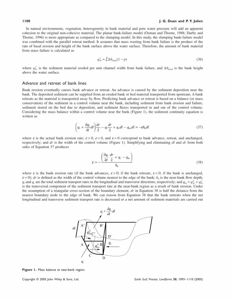
Advance and retreat of bank linesBank erosion eventually causes bank advance or retreat. An advance is caused by the sediment deposition near thebank. The deposited sediment can be supplied from an eroded bank or bed material transported from upstream. A bankretreats as the material is transported away by flow. Predicting bank advance or retreat is based on a balance (or massconservation) of the sediment in a control volume near the bank, including sediment from bank erosion and failure,sediment stored on the bed due to deposition, and sediment fluxes transported in and out of the control volume.Considering the mass balance within a control volume near the bank (Figure 1), the sediment continuity equation iswritten as

qq

ldl

drq

drq dl q dl h dll

ll r br b +

∂∂

− + − = −2 2

ε (37)

where ε is the actual bank erosion rate; ε > 0, ε < 0, and ε = 0 correspond to bank advance, retreat, and unchanged,respectively; and dr is the width of the control volume (Figure 1). Simplifying and eliminating dl and dr from bothsides of Equation 37 produces

ε

= −

∂∂

+ −

q

l

drq q

h

lr br

b

2(38)

where ε is the bank erosion rate (if the bank advances, ε > 0; if the bank retreats, ε < 0; if the bank is unchanged,ε = 0); dr is defined as the width of the control volume nearest to the edge of the bank; hb is the near-bank flow depth;ql and qr are the total sediment transport rates in the longitudinal and transverse directions, respectively; and qbr = qb

br + q fbr

is the transversal component of the sediment transport rate at the near-bank region as a result of bank erosion. Underthe assumption of a triangular cross-section of the boundary element, dr in Equation 38 is half the distance from thenearest boundary node to the edge of bank. We can reason from Equation 38 that the bank retreats when the netlongitudinal and transverse sediment transport rate is decreased or a net amount of sediment materials are carried out

Figure 1. Mass balance at near-bank region.



of a control volume near the bank. Conversely, if the net sediment transport to the control volume is increased, thebank will advance. The variable dr is defined as the width of the control volume adjacent to the bank.

Comparing with the Ikeda et al. (1981) bank erosion model, the bank erosion rate in the present study is determinedby the flow and sediment conditions near the bank rather than by only excess velocity. Accordingly, the movement ofa bank is only related to the near-bank flow field. If the excess near-bank velocity is greater than zero, the bank willretreat. Equation 38 considers sediment transport fluxes, and one can see that even when flow velocity and shear stressnear the bank are high, the bank may not retreat, because a net sediment flux may be transporting into the controlvolume adjacent to the bank.

Numerical Methods

The ‘efficient element method’ (Wang and Hu, 1990) is used to solve the momentum and continuity equations. Thenumerical technique was originally a collocated, weighted residual finite element method. The traditional Lagrangianinterpolation function is employed to discretize the linear terms in Equations 1, 2, and 3. To address adequately theupwinding effect, another set of interpolating functions is derived based on the solution of the convection anddiffusion equation to discretize non-linear terms (advection terms) in the flow momentum equations. These two sets ofshape functions are transformed to the shape function for global elements based on the isoparametric mappingapproach. A detailed description of the numerical scheme for the flow hydrodynamic model can be found in Duan(2004).

The sediment continuity equation (Equation 33) is discretized using the Lagrangian interpolation shape functions. Abackward finite difference scheme is used for the time derivative term. The discretized form of Equation 33 is

( )

1 01

1

9

1

9

−−

+∂∂

+∂∂

=−

= =∑ ∑p

z z

t xq

yqb

tbt

i

ixi

i

iyi∆

ϕ ϕ(39)

where ϕi is the shape function with the superscription denoting the time step, and the subscription denoting the nodenumber. In the present study, flow and bed deformation computations are decoupled. Sediment transport rates arecalculated after flow has reached a steady state. Then, Equation 39 is solved to obtain a new bed elevation. The timestep of sediment computation is selected such that bed-elevation changes are less than 2 per cent of the flow depth.

Besides calculating bed-elevation changes, bank lines are also adjusted according to the rate of bank erosion.Figure 2 illustrates the calculation with Equation 38 for the bank advance and retreat rate at the elements adjacent to

Figure 2. Movement of nodes at banks.



the bank. The boundary nodes are (1, j) and (1, j + 1), and the adjacent internal nodes are (2, j) and (2, j + 1). Equation38 is solved at node (1, j) to obtain the bank erosion rate at the edge of bank B. The boundary element used toevaluate the bank erosion rate is a prism-like, three-dimensional element with a triangular cross-section ABC. Thebank erosion rate at node (1, j) is assumed to be the same as that at the edge of bank B, which can be expressed as

εi jl l

r br

r q j q j

lq j q j,

( , ) ( , ) ( , ) ( , )=

− +− +

∆∆2

2 2 12 1 (40)

where ∆r is the distance between B and C. As a boundary condition, the longitudinal component of the sedimenttransport rate at node (1, j) is assumed to be the same as the adjacent internal node (2, j). Using Equations 35 and 36,the expression qbr(i, j) = qb

br(i, j) + q fbr(i, j) is calculated. According to the bank erosion rate, each boundary node is

moved the distance of ∆B1, j

∆B1, j = ε1, j∆tbank (41)

where ∆tbank is the bank erosion time step. In Figure 2, (1′, j) and (1′, j + 1) are the boundary nodes after bank erosion,and the hatched area represents the eroded material. At the inlet section, the bank erosion rate is assumed to be zero.At the outlet section, the bank erosion rate is assumed to be the same as in the adjacent upstream section.

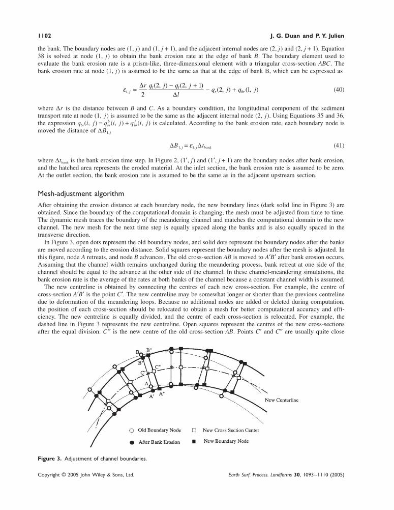
Mesh-adjustment algorithmAfter obtaining the erosion distance at each boundary node, the new boundary lines (dark solid line in Figure 3) areobtained. Since the boundary of the computational domain is changing, the mesh must be adjusted from time to time.The dynamic mesh traces the boundary of the meandering channel and matches the computational domain to the newchannel. The new mesh for the next time step is equally spaced along the banks and is also equally spaced in thetransverse direction.

In Figure 3, open dots represent the old boundary nodes, and solid dots represent the boundary nodes after the banksare moved according to the erosion distance. Solid squares represent the boundary nodes after the mesh is adjusted. Inthis figure, node A retreats, and node B advances. The old cross-section AB is moved to A′B′ after bank erosion occurs.Assuming that the channel width remains unchanged during the meandering process, bank retreat at one side of thechannel should be equal to the advance at the other side of the channel. In these channel-meandering simulations, thebank erosion rate is the average of the rates at both banks of the channel because a constant channel width is assumed.

The new centreline is obtained by connecting the centres of each new cross-section. For example, the centre ofcross-section A′B′ is the point C′. The new centreline may be somewhat longer or shorter than the previous centrelinedue to deformation of the meandering loops. Because no additional nodes are added or deleted during computation,the position of each cross-section should be relocated to obtain a mesh for better computational accuracy and effi-ciency. The new centreline is equally divided, and the centre of each cross-section is relocated. For example, thedashed line in Figure 3 represents the new centreline. Open squares represent the centres of the new cross-sectionsafter the equal division. C″ is the new centre of the old cross-section AB. Points C′ and C″ are usually quite close

Figure 3. Adjustment of channel boundaries.



because the bank is only restricted to move a distance of less than 2 per cent of the channel width at each time step.In the case of a high erosion rate, the time step of bank erosion must be reduced. The adjusted cross-section A″B″ mustbe normal to the new centreline at C″ and have a width equal to the initial channel width AB. Then, for each cross-section, computational nodes along the transverse direction are uniformly distributed. The adjusted mesh has the samecomputational domain as the previous one, even though the positions of cross-sections and computational nodes havebeen relocated in the physical domain. Each new cross-section of the adjusted mesh is normal to the new centreline,and computational nodes are uniformly distributed along the transverse direction.

Since the computational nodes do not move considerably in each time step, bed elevation at any node in the newmesh is interpolated according to the bed elevation of the adjacent upstream and downstream nodes in the old mesh.After the mesh is adjusted, the flow field must be recalculated for a certain time to achieve a steady state in the newchannel. This entire process is repeated for each new morphological time step until the simulation is completed at thespecified time step. Since boundary nodes move less than 2 per cent during each time step, the error due to interpola-tion is assumed negligible.

Test and Verification

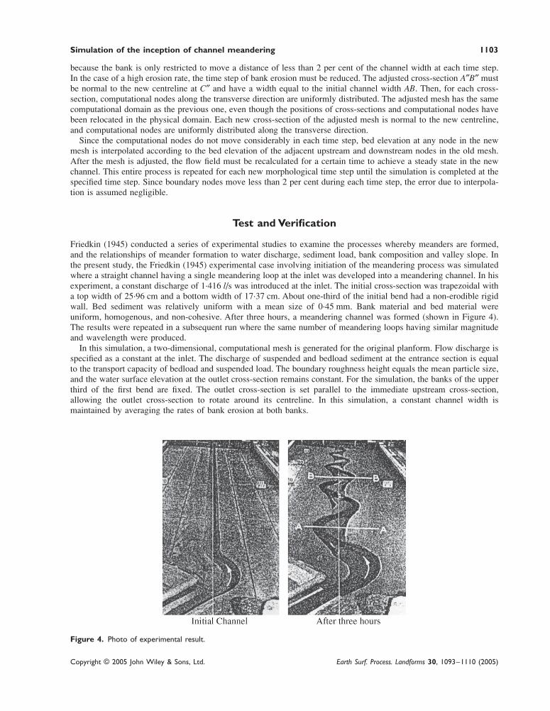
Friedkin (1945) conducted a series of experimental studies to examine the processes whereby meanders are formed,and the relationships of meander formation to water discharge, sediment load, bank composition and valley slope. Inthe present study, the Friedkin (1945) experimental case involving initiation of the meandering process was simulatedwhere a straight channel having a single meandering loop at the inlet was developed into a meandering channel. In hisexperiment, a constant discharge of 1·416 l/s was introduced at the inlet. The initial cross-section was trapezoidal witha top width of 25·96 cm and a bottom width of 17·37 cm. About one-third of the initial bend had a non-erodible rigidwall. Bed sediment was relatively uniform with a mean size of 0·45 mm. Bank material and bed material wereuniform, homogenous, and non-cohesive. After three hours, a meandering channel was formed (shown in Figure 4).The results were repeated in a subsequent run where the same number of meandering loops having similar magnitudeand wavelength were produced.

In this simulation, a two-dimensional, computational mesh is generated for the original planform. Flow discharge isspecified as a constant at the inlet. The discharge of suspended and bedload sediment at the entrance section is equalto the transport capacity of bedload and suspended load. The boundary roughness height equals the mean particle size,and the water surface elevation at the outlet cross-section remains constant. For the simulation, the banks of the upperthird of the first bend are fixed. The outlet cross-section is set parallel to the immediate upstream cross-section,allowing the outlet cross-section to rotate around its centreline. In this simulation, a constant channel width ismaintained by averaging the rates of bank erosion at both banks.

Figure 4. Photo of experimental result.



Figure 5. Changes in computational meshes during the meander-forming processes.

Adjustments to the computational meshes made during the simulation are plotted in Figure 5; the top diagramillustrates the original mesh, and the bottom one illustrates the mesh of the completely developed meandering channel.The present model requires the total number of cross-sections and nodes in each cross-section to remain unchanged, sothe distance between cross-sections increases as the channel length increases. In this model run, the initial aspect ratioof the finite element mesh is 1:4, and the aspect ratio of the developed meandering channel is 1:7, which satisfy theconvergence criteria for the hydrodynamic model (Duan, 2004). After each mesh adjustment, the flow field is recalcu-lated as the initial condition by using flow solutions from previous time steps.

The simulated flow field is plotted in Figure 6. It includes the flow velocity vector, and surface elevation occurringduring the meander-forming process. The flow depth is very shallow, and velocity is low in areas outside the compu-tational domain; consequently, the present model assumes that sediment transport in these areas is negligible. At thebeginning of the simulation (T = 0 h), the initial meandering loop causes a redistribution of flow momentum. As timeprogresses, sand bars develop near the inner bank of the initial loop and at the location where the initial loop connectswith the straight reach. At T = 0·5 h the primary flow course becomes wave-like because sand bars form in the straightreach. This wave-like flow pattern facilitates the development of sand bars, and at T = 2·0 h, a fully developedmeandering loop occurs in the straight reach. Two additional meandering loops are fully developed at T = 3·0 h.

High-velocity zones are observed near the inner bank at the beginning of the simulation. These zones gradually shiftto the outer bank as the transverse bed slope increases due to the presence of sand bars. Parker (1984) and Dietrichand Smith (1983) attributed this phenomenon to the secondary flow generated by bed topography. Simulation resultsindicate that the initial meandering loop propagates downstream through the formation of sand bars, resulting in ameandering flow path. Apparently, because of the uniform bed and bank material, the initial bend can be transmittedalmost perfectly downstream, producing a series of uniform bends. After the meandering process reaches equilibrium,a series of almost identical sand bars resides on the inside of bends.

The simulated bed elevations for the stages in the meandering process are plotted in Figure 7. Simulation resultsshow that the generation of alternate bars occurs at both sides of the channel. The channel begins meandering after thealternate bars are formed. As time progresses, the meandering amplitude and wavelength increase gradually. Friedkin(1945) states that bends develop as flow impinges on the bank and erodes bank material, then deposits the material onthe inside of the bend. Super-elevation on concave banks of this low-sinuosity stream is observed in the experiment.



Figure 6. Simulated flow field including velocity and surface elevation. This figure is available in colour online atwww.interscience.wiley.com/journal/espl

Super-elevation of flow near the concave bank increases as the meandering process evolves, indicating that secondaryflow becomes stronger as sinuosity increases. The amplitude and wavelength of the formed meandering stream arevery close to experimental observations as shown in Figure 4.

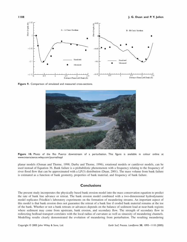
Longitudinal profiles representing the various stages in the meandering process at the inner, outer and centrelinelocations are plotted in Figure 8. This observation is verified by numerous field observations where the slope ofalluvial channels decreases as meandering develops. Because the cross-sections are deep along the concave banks ofthe bends and shallow in the crossings between the bends (plotted in Figure 9), the longitudinal profiles at thecentreline consist of a series of deep, separated by shallow, crossings. At the apex where the concave bank exists,triangular-shaped cross-sections are formed (Figure 9), which agrees very well with field measurements (e.g. Julien,2002; Julien and Anthony, 2002).

Sediment, including suspended load and bedload, was fed at the entrance. The simulation shows that sediment frombank erosion replenishes sediment deposited on sand bars. Trading sediment from the main channel with sedimentfrom bank erosion consequently results in downstream aggragation. In the present study, we also observed that the



differences between bed elevations at the inner and outer banks increase with the formation of meandering channels,which indicates that the transverse bed slope increases as the meandering process evolves.

The simulated meandering planform and cross-sections are very close to the experimental results. This indicatesthat the present model is capable of predicting the formation of alternate bars from a single perturbation in a straightreach of a channel. This two-dimensional model also adequately simulates the initiation of channel meandering.

Discussion

An example from the Rio Puerco in New Mexico is shown in Figure 10. Accordingly, a straight channel wasexcavated with a vertical drop (about 2 m) in sandstone in order to prevent lateral migration and eventual impinge-ment of the channel into the nearby road embankment. The elevation drop triggered a slight lateral perturbation of thesystem and the downstream portion of the channel started to meander. The features of the channel shown in Figure 10are quite similar to the features obtained by the model. Essentially, the amplitude of meandering decreases in thedownstream direction. The resulting channel features are very similar to those described by the model in Figure 7.

Natural meandering streams commonly have cohesive banks (Knighton and Nanson, 1993; Millar, 2000). Retreat ofcohesive bank lines is a complex process consisting of fluvial erosion, bank failure, weathering, piping or sapping.Bank failure can dominate bank erosion processes involving cohesive bank material, and algorithms for mass failureare available for cohesive banks (Darby and Delbono, 2002). Bank failure models for cohesive bank material, such as

Figure 7. Initiation of a meandering channel from a straight channel. This figure is available in colour online atwww.interscience.wiley.com/journal/espl



Figure 8. Changes in longitudinal bed slopes with time. This figure is available in colour online at www.interscience.wiley.com/journal/espl



planar models (Osman and Thorne, 1998; Darby and Thorne, 1996), rotational models or cantilever models, can beused instead of Equation 36. Bank failure is a probabilistic phenomenon with a frequency relating to the frequency ofriver flood flow that can be approximated with a LP(3) distribution (Duan, 2001). The mass volume from bank failureis estimated as a function of bank geometry, properties of bank material, and frequency of bank failure.

Conclusions

The present study incorporates the physically based bank erosion model into the mass conservation equation to predictthe rate of bank line advance or retreat. The bank erosion model combined with a two-dimensional hydrodynamicmodel replicates Friedkin’s laboratory experiments on the formation of meandering streams. An important aspect ofthis model is that bank erosion does not guarantee the retreat of a bank line if eroded bank material remains at the toeof the bank. Whether or not a bank retreats or advances depends on the balance of sediment load at near-bank regionswhere sediment may come from upstream, bank erosion, and secondary flow. The strength of secondary flow inredirecting bedload transport correlates with the local radius of curvature as well as sinuosity of meandering channels.Modelling results clearly demonstrated the evolution of meandering from perturbation. The resulting meandering

Figure 9. Comparison of simulated and measured cross-sections.

Figure 10. Photo of the Rio Puerco downstream of a perturbation. This figure is available in colour online atwww.interscience.wiley.com/journal/espl



channel has almost uniform loops, and the location and size of the sand bars are similar to the experimental observa-tions. The essential processes leading to meander formation are well replicated with this model. Additionally, model-ling results also indicated that suspended sediment is less important in modelling meander migration, while bankerosion and bedload transport play significant roles in the meandering evolution process. The growth of sand barsdetermines the hydrodynamic flow field that pushes towards the concaving banks. Bank material from the cavingbanks will supplement sediment deposits on point bars when bed and bank material are the same, such as in thelaboratory experiments. At this point, this model properly simulates key laboratory experiments of channel meander-ing. It is also very similar to some features observed in the field, such as observed on the Rio Puerco in New Mexico.This model enhances the current capability in modelling natural morphodynamic processes. This also contributes tobetter understanding of the processes of lateral channel migration and helps explain the formation of river meanders.

AcknowledgementsThis work is a result of research sponsored by the US Department of Defense Army Research Office under Grant NumberDAAD19-00-1-0157, and by a Cooperative Agreement between the US Army Corps of Engineers and Desert Research Institute(DRI), under Grant Number DACW42-03-0-0003. Thanks to Ms Jennifer Lease for her help in proofreading this manuscript.

References

ASCE Task Committee. 1998. River width adjustment. I: Processes and mechanisms. Journal of Hydraulic Engineering 124(9): 881–902.Bormann N, Julien PY. 1990. Scour downstream of grade-control structures. Journal of Hydraulic Engineering 117(5): 579–594.Bridge JS. 1992. A revised model for water flow, sediment transport, bed topography and grain size sorting in natural river bends. Water

Resources Research 28: 999–1013.Chien N, Wan ZH. 1991. Dynamics of Sediment Transport. Academic Press of China: Beijing 563–576; (in Chinese).Crosato A. 1990. Simulation of meandering river processes. In Communications on Hydraulic and Geotechnical Engineering. Delft Univer-

sity of Technology: Delft, The Netherlands.Darby S, Delbono I. 2002. A model of equilibrium bed topography for mean bends with erodible banks. Earth Surface Processes and

Landforms 27(10): 1057–1085.Darby SE, Thorne CR. 1996. Development and testing of riverbank-stability analysis. Journal of Hydraulic Engineering 122(8): 443–454.Darby SE, Alabyan AM, Van De Wiel MJ. 2002. Numerical simulation of bank erosion and channel migration in meandering rivers. Water

Resources Research 38(9): 1163. DOI: 10.1029/2001WR000602Dietrich W, Smith JD. 1983. Influence of the point bar on flow through curved channels. Water Resources. Research 19: 1173–1192.Duan JG. 2001. Simulation of streambank erosion processes with a two-dimensional numerical model. In Landscape Erosion and Evolution

Modelling, Harmon RS, Doe WW III (eds). Kluwer Academic/Plenum Publishers: New York; 389–427.Duan JG. 2004. Simulation of flow and mass dispersion in meandering channels. Journal of Hydraulic Engineering 130(10): 964–976.Duan JG, Wang SSY, Jia Y. 2001. The application of the enhanced CCHE2D model to study the alluvial channel migration processes.

Journal of Hydraulic Research 39(5): 469–480.Engelund F. 1974. Flow and bed topography in channel bend. Journal of Hydraulic Division 100(11): 1631–1648.Friedkin J. 1945. A Laboratory Study of the Meandering of Alluvial Rivers. US Waterways Experiment Station: Vicksburg.Hooke JM. 1995. River channel adjustment to meander cutoffs on the River Bollin and River Dane. Geomorphology 14: 235–253.Ikeda S. 1989. Sediment transport and sorting at bends. In River Meandering, Ikeda S, Parker G (eds). American Society of Civil Engineers:

New York; 103–115.Ikeda S, Parker G, Sawai K. 1981. Bend theory of river meanders, 1, Linear development. Journal of Fluid Mechanics 112: 363–377.Ikeda S, Nishimura T. 1986. Flow and bed profile in meandering sand-silt rivers. Journal of Hydraulic Engineering 112(7): 562–579.Johannesson H. 1985. Computer Simulation of Migration of Meandering Rivers. Dissertation, University of Minnesota, St. Paul.Julien PY. 2002. River Mechanics. Cambridge University Press: Cambridge.Julien PY, Anthony DJ. 2002. Bedload motion and grain sorting in a meandering stream, Journal of Hydraulic Research 40(2): 125–133.Kikkawa H, Ikeda S, Kitagawa A. 1976. Flow and bed topography in curved open channels. Journal of Hydraulic Division 102(9): 1327–

1342.Knighton AD, Nanson GC. 1993. Anastomosis and the continuum of channel pattern. Earth Surface Processes and Landforms 18: 613–625.Lan YQ. 1990. Dynamic Modelling of Meandering Alluvial Channels. Dissertation, Colorado State University, Fort Collins.Lancaster ST, Bras RL. 2002. A simple model of river meandering and its comparison to natural channels. Hydrological Processes 16(1): 1–

26.Millar RG. 2000. Influence of bank vegetation on alluvial channel patterns. Water Resources Research 36: 1109–1118.Mosselman E. 1998. Morphological modelling of rivers with erodible banks. Hydrological Processes 12: 1357–1370.Nagata N, Hosoda T, Muramoto Y. 2000. Numerical analysis of river channel processes with bank erosion. Journal of Hydraulic Engineer-

ing 126(4): 243–252.Nicholas AP, Smith GHS. 1999. Numerical simulation of three-dimensional flow hydraulics in a braided channel. Hydrologic Processes 13:

913–929.



Odgaard A. 1989a. River meander model, I: Development. Journal of Hydraulic Engineering 115(11): 1433–1450.Odgaard A. 1989b. River meander model, II: Application. Journal of Hydraulic Engineering 115(11): 1450–1464.Olsen NRB. 2003. Three-dimensional CFD modelling of self-forming meandering channel. Journal of Hydraulic Engineering 129(5): 366–

372.Osman MA, Thorne CR. 1988. Riverbank stability analysis. I: Theory. Journal of Hydraulic Engineering 114(2): 134–150.Parker G. 1984. Lateral bedload transport on side slope. Journal of Hydraulic Engineering 110: 197–199.Parker G, Andrews ED. 1986. On the time development of meander bends. Journal of Fluid Mechanics 162: 139–156.Pizzuto JE. 1990. Numerical simulation of gravel river widening. Water Resources Research 26: 1971–1980.Sun T, Meakin P, Jossang T, Schwarz K. 1996. A simulation model for meandering rivers. Water Resources Research 32: 2937–2954.Sun T, Meakin P, Jossang T. 2001a. A computer model for meandering rivers with multiple bedload sediment sizes. 1. Theory. Water

Resources Research 37(8): 2227–2241.Sun T, Meakin P, Jossang T. 2001b. A computer model for meandering rivers with multiple bedload sediment sizes 2. Computer simulations.

Water Resources Research 37(8): 2243–2258.Van Rijn LC. 1989. Sediment transport by currents and waves. Technical Report H461. Delft Hydraulics: Delft, The Netherlands.Wang SS, Hu K. 1990. Improved methodology for formulating finite element hydrodynamic models. In Finite Elements in Fluids, Volume 8,

Chung T (ed.). Hemisphere Publishing: New York; 1127–1134.

Documents

Numerical simulation of the inception of channel meandering