NUMERICAL MODELING OF DYNAMIC SOIL-PILE-STRUCTURE

INTERACTION

By

SURENDRAN BALENDRA

A thesis submitted in partial fulfillment of the requirements for the degree of

MASTER OF SCIENCE IN CIVIL ENGINEERING

WASHINGTON STATE UNIVERSITY Department of Civil and Environmental Engineering

December 2005

To the Faculty of Washington State University:

The members of the Committee appointed to examine the thesis of

SURENDRAN BALENDRA find it satisfactory and recommend that it be accepted.

Chair

ii

ACKNOWLEDGEMENTS

I would like to express my sincere gratitude to my advisor Dr. Adrian Rodriguez-

Marek for his tireless guidance, boundless patience and continuous support rendered

throughout the entire project. His expert knowledge in this field is the foundation for the

successful completion of the project.

Special thanks are extended to the Department of Civil and Environmental

Engineering, Washington State University and to Washington State Department of

Transportation under the Grant Number T2696-02 for granting the funds for the

successful completion of my Masters.

I am deeply obliged to Dr. Balasingam Muhunthan and Dr. William Cofer for

being my Master’s Committee members and guiding me at appropriate time through their

precious suggestions. My special thanks to Dr. Balasingam Muhunthan for inspiring me

to do a Master’s in Geotechnical engineering and guiding me in all aspects throughout

my course of study. I would also like to extend my thanks to Drs Laith Tashman, Thomas

Papagiannakis, Abdullah Assa’ad, and Francisco Manzo-Robledo for contributing to my

overall education at Washington State University.

I also appreciate Tom Weber for assisting me in computer resource management

and Vicki Ruddick for assisting me in the secretarial works.

I would like to thank all my friends and colleagues for their kindness and co-

operation, especially Sasi, Sathish and Senthil for their help in many aspects. I also like

to extend my thanks to my undergraduate friends Balakumar, Mathiyarasan, Naventhan

iii

and Pirahas for their continuous support in the course of study. My sincere thanks to my

High School mathematics teacher Rajeskanthan for inculcating the fire in me.

Last but not least, special thanks to my relatives especially, Aravinthan (Ravi),

Partheepan and Vasantha. Also, thanks to my parents, brother, and sister whose prayers

have helped me in successful completion of the program.

iv

NUMERICAL MODELING OF DYNAMIC SOIL-PILE-STRUCTURE INTERACTION

Abstract

By Surendran Balendra, M.S.

Washington State University

December 2005

Chair: Adrian Rodriguez-Marek

The analysis of structures subject to earthquake ground motions must properly

account for the interaction between the foundation and the superstructure. The passage of

seismic waves through the foundation affects the ground motion at the base of the

structure and generates stresses on foundation elements. This effect is termed kinematic

interaction and its effects on the ground motion are described by a function termed the

transfer function. On the other hand, the response of a structure is a function of the

foundation compliance, and, in turn, inertial forces resulting from structural response

affect the stresses on foundation elements. This interaction is termed inertial interaction

and is captured by representing the foundation through an impedance function. In this

study, numerical models using ABAQUS were developed to study both inertial and

kinematic effects. The focus of this study was to perform parametric studies on the

various variables that affect kinematic transfer functions and inertial impedance functions

of pile foundations. The independent variables of this parametric study were material

nonlinearity, soil-pile separation, pile diameter, intensity of the input motion, and the

v

inertial force magnitude. A bounding surface plasticity soil model is used in this study to

model soil nonlinearity. Issues related to the numerical modeling of soil-pile-structure

interaction are discussed at length, including the application of dynamic loading as a

shear stress time history, the development of user-defined pile-soil interface models, and

the treatment of infinite and absorbing boundaries for the lateral and bottom boundaries,

respectively. The model was validated by comparison with analytical solutions and

previously published results.

Results for a fixed head single pile in a plastic soil show that soil nonlinearity

reduces the amplitude of the transfer function significantly for high frequencies; however,

the intensity of the ground motion does not affect significantly the kinematic transfer

function. Soil-pile separation has no effect on the kinematic transfer functions but has a

considerable effect on the impedance function. Normal stress due to kinematic effects

attains a maximum when the loading frequency coincides with the frequency

corresponding to the resonant frequency of the soil column (e.g., the site frequency). The

maximum kinematic stress on flexible piles occurs at the depth of a stiffness contrast

between soil layers. For rigid piles, maximum kinematic stresses occur at the pile head.

The presence of an interface between hard and soft soil has no effect on stresses due to

inertial interaction for flexible piles and has considerable effect on inertial stresses for

rigid piles. Soil-pile separation results in an increase of both kinematic and inertial

stresses in the pile.

vi

TABLE OF CONTENTS

Page

ACKNOWLEDGEMENTS iii

ABSTRACT v

LIST OF TABLES xii

LIST OF FIGURES xiii

CHAPTER 1 INTRODUCTION

1.1 BACKGROUND 1

1.2 OBJECTIVES 4

1.3 ORGANIZATION OF THE THESIS 5

CHAPTER 2 LITERATURE REVIEW

2.1 INTRODUCTION 6

2.2 SOIL-PILE-STRUCTURE INTERACTION ANALYSES – THE

APPROACH

6

2.2.1 SPSI analyses procedure for design 7

Kinematic interaction 9

Inertial interaction 10

2.2.2 Numerical tools 12

2.3 FINITE ELEMENT METHOD APPLIED TO SPSI PROBLEMS 13

2.3.1 Boundary conditions 13

Kelvin element 14

Viscous element (dashpot element) 15

vii

Infinite elements 15

2.3.2 Soil-pile interface 16

2.3.3 Loading 17

2.3.4 Soil behavior 17

2.3.5 Applications 17

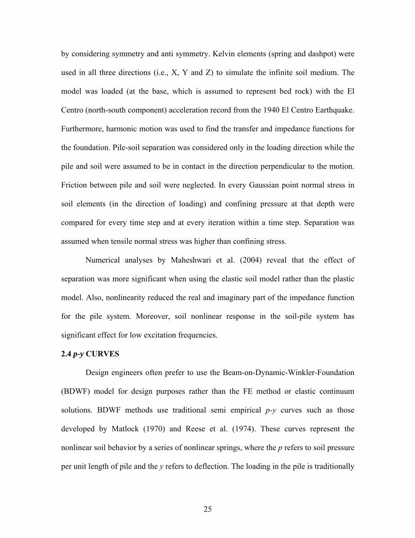
2.4 p-y CURVES 25

2.4.1 Existing p-y curves 27

2.4.1.1 Soft clay p-y curves 28

2.4.1.2 Stiff clay p-y curves below the water table 29

2.4.1.3 Stiff clay p-y curves above the water table 31

2.4.1.4 Sand p-y curves 31

2.4.1.5 API sand p-y curves 34

2.4.1.6 p-y curves for φ−c soils 35

2.4.2 Effect of pile diameter on p-y curves 36

2.4.3 Back calculation of p-y curves 37

CHAPTER 3 NUMERICAL MODELING

3.1 INTRODUCTION 44

3.2 CONSTITUTIVE SOIL MODEL 44

3.2.1 General description 45

3.2.2 Mathematical formulation 47

3.2.3 Hardening function 49

3.2.4 Loading and unloading conditions 50

3.2.5 Rayleigh’s damping 51

viii

3.2.6 Model parameters 53

3.3 INTERFACE MODEL 54

3.4 TRANSMITTING BOUNDARY CONDITION 57

3.4.1 Free-field boundaries 57

3.4.2 Quiet (viscous) boundaries 59

3.5 LOADING 60

3.6 MODEL VALIDATION 60

3.6.1 Validation of the load application method 61

3.6.2 Stiffness proportional damping validation 64

3.6.3 Validation of pile element size 65

3.6.4 Validation of model size 67

3.6.5 Validation of model for pile-soil interaction 70

CHAPTER 4 PARAMETRIC STUDY ON KINEMATIC INTERACTION

4.1 INTRODUCTION 73

4.2 COMPUTATION OF THE TRANSFER FUNCTION 73

4.3 MODEL DESCRIPTION 74

4.4 SINGLE PILE: HARMONIC EXCITATION AT THE BASE 76

4.4.1 Effect of non-linearity of the soil in transfer function 77

4.4.2 Effect of ground motion intensity in transfer function 78

4.4.3 Effect of pile diameter on the transfer function 80

4.4.4 Effect of gapping (pile-soil separation) on the transfer

function

83

4.5 KINEMATIC STRESS IN A SINGLE PILE 84

ix

4.5.1 Effect of soil non-linearity on kinematic stress 85

4.5.2 Effect of pile diameter on kinematic stress 87

4.5.3 Effect of gapping (pile-soil separation) on kinematic stresses 91

CHAPTER 5 PARAMETRIC STUDY ON INERTIAL INTERACTION

5.1 INTRODUCTION 93

5.2 COMPUTATION OF THE IMPEDANCE FUNCTION 93

5.3 MODEL DESCRIPTION 94

5.4 SINGLE PILE: HARMONIC EXCITATION AT THE TOP OF THE

PILE

94

5.4.1 Effect of non-linearity of the soil on the impedance function 95

5.4.2 Effect of driving force magnitude on the impedance function 97

5.4.3 Effect of pile diameter on the Impedance Function 99

5.4.4 Effect of gapping (pile-soil separation) on the impedance

function

102

5.5 INERTIAL STRESS IN A SINGLE PILE 104

5.5.1 Effect of Soil non-linearity on inertial stress 104

5.5.2 Effect of pile diameter on inertial stress 106

5.5.3 Effect of gapping (pile-soil separation) on inertial stresses 110

CHAPTER 6 CONCLUSIONS AND RECOMMENDATIONS

6.1 SUMMARY 112

6.2 CONCLUSIONS 113

6.2.1 Kinematic interaction 113

6.2.2 Inertial interaction 115

x

6.3 RECOMMENDATION FOR FUTURE RESEARCH 117

REFERENCES 118

xi

LIST OF TABLES

Page

Table 2.1 Summary of procedure in developing soft clay p-y curves (Matlock,

1970)

38

Table 2.2 Summary of procedure in developing stiff clay with free water p-y

curves (Reese et al., 1975)

39

Table 2.3 Summary of procedure in developing stiff clay with free water p-y

curves (Welch and Reese, 1972; and Reese Welch, 1975)

40

Table 2.4 Summary of procedure in developing sand p-y curves (Reese et al.,

1974)

41

Table 2.5 Summary of procedure in developing API sand p-y curves (API, 1987) 42

Table 2.6 Summary of procedure in developing cemented sand p-y curves

(Ismael, 1990)

43

Table 3.1 Properties used in the FE models in validation of model size analysis 68

Table 4.1 Elastic properties used in the FE models in parametric studies 76

Table 4.2 Borja’s model parameters used in the FE models in parametric studies 76

Table 4.3 TF for 0.5m wide pile with different intensity of input ground motion.

Input motion frequency is 10 Hz

79

Table 4.4 TF for 0.5 m wide pile with different interface with 10 Hz harmonic

wave

84

Table 5.1 Static load to cause a pile to a deflection of 25 mm (ultimate load) 95

xii

LIST OF FIGURES

Page

Figure 2.1 Sketch of SPSI problems (after Gazetas and Mylonakis 1998) 8

Figure 2.2 The superposition theorem for SPSI problems (after Gazetas and

Mylonakis 1998)

9

Figure 2.3 Quasi 3-D model of pile-soil response (after Wu 1994) 19

Figure 2.4 Outline of the structure and pile foundation (from Cai et al. 2000) 20

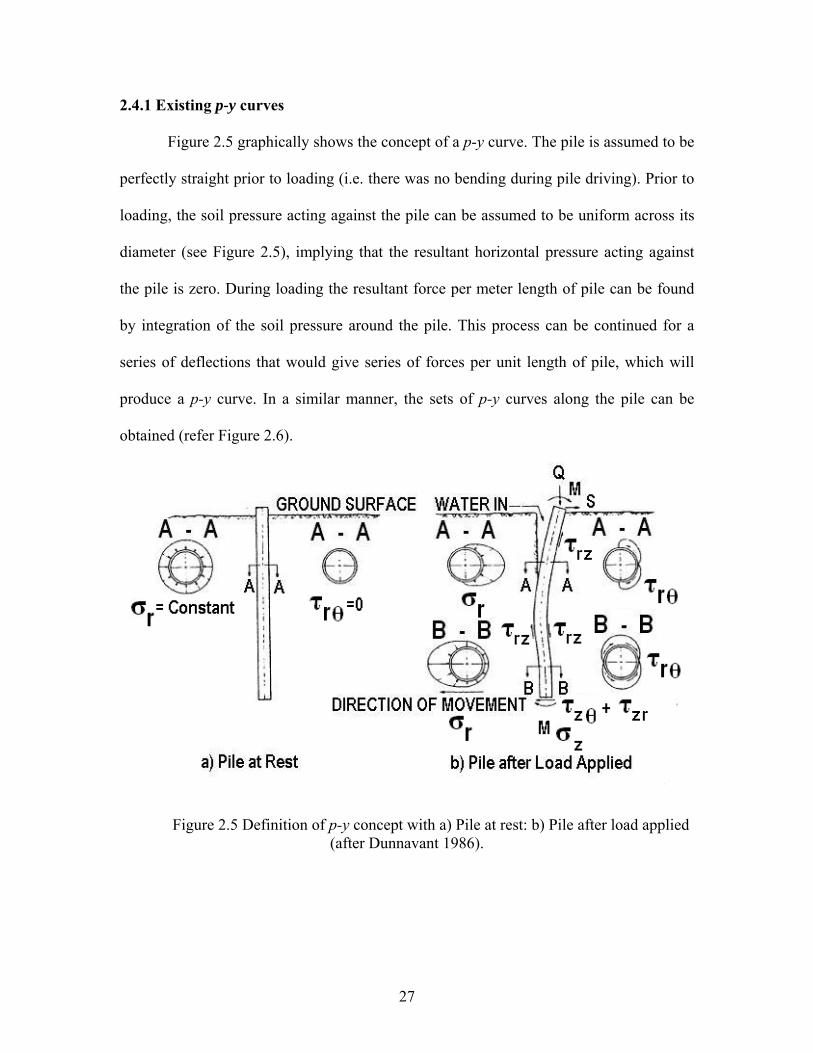
Figure 2.5 Definition of p-y concept with a) Pile at rest: b) Pile after load applied

(after Dunnavant 1986)

27

Figure 2.6 Typical family of p-y curves response to lateral loading (after

Dunnavant 1986)

28

Figure 2.7 Characteristic shape of p-y curve for soft Clay a) Static loading: b)

Cyclic loading (after Matlock 1970)

29

Figure 2.8 Characteristic shape of p-y curve for stiff clay below water table for a)

Static loading: b) Cyclic loading: c) Value of constant A (after Reese

et al. 1975)

30

Figure 2.9 Characteristic shape of p-y curve for stiff clay above the water table

for a) Static loading: b) Cyclic loading (Welch and Reese 1972,

Reese and Welch 1975)

31

Figure 2.10 Characteristic shape of p-y curves for sand (Reese et al. 1974) 32

Figure 2.11 Values of coefficient A used for developing p-y curves for sand a)

Coefficient A; b) Coefficient B (after Reese et al. 1974)

33

xiii

Figure 2.12 Charts used for developing API sand p-y curves (API 1987) 34

Figure 2.13 Characteristic shapes of p-y curves for sand (Reese et al. 1974) 36

Figure 3.1 Schematic diagram of the bounding surface plasticity model showing

unloading point Fo, yield surface F, and bounding surface B on the π

plane. Contours of constant H′ are centered about Fo, H′ is infinite at

Fo and decreases to Ho on the surface B (adapted from Borja and

Amies 1994)

47

Figure 3.2 Relationship between rayleigh damping and frequency 53

Figure 3.3 Schematic diagrams of dashpot arrangements of free field boundaries

and the quiet boundary at the base of the model (adapted from FLAC

3D 2002)

59

Figure 3.4 FE soil column model. 63

Figure 3.5 Comparison of TF for between FE analysis and an analytical solution 63

Figure 3.6 Comparison of response from a built-in ABAQUS elastic constitutive

material with built-in stiffness proportional damping and user defined

(umat) elastic material

65

Figure 3.7 Comparison of displacement for different size element with

predictions of beam theory analysis

67

Figure 3.8 Normalized pile top response for varying “a” values 69

Figure 3.9 Normalized pile top response for varying “b” values 69

Figure 3.10 FE soil-pile model 71

Figure 3.11 Real part of the impedance function obtained from FEA 72

xiv

Figure 3.12 Lateral dynamic stiffness versus frequency from 3D FEA (after

Gazetas and Dobry 1984)

72

Figure 4.1 Sketch of single-pile system subject to vertically propagating shear

waves (adapted from Fan et al. 1991)

74

Figure 4.2 FE mesh for the analysis of the single, fixed head pile under dynamic

loading with perfect bonding between pile and soil surface

75

Figure 4.3 Variation with frequency of the transfer function of a single fixed

head pile for horizontal displacement for varying diameters

78

Figure 4.4 Octahedral shear stress shear versus octahedral shear strain curve

obtained for an element close to the pile and for different intensities

of the input ground motion

79

Figure 4.5 Variation of transfer function of single fixed head pile for horizontal

displacement with non-dimensional frequency for varying diameters

for elastic soil

80

Figure 4.6 Variation of transfer function of single fixed head pile for horizontal

displacement with frequency for varying diameters for elastic soil

81

Figure 4.7 Variation of transfer function of single fixed head pile for horizontal

displacement with non-dimensional frequency for varying diameters

for plastic soil

82

Figure 4.8 Variation of transfer function of single fixed head pile for horizontal

displacement with frequency for varying diameters for plastic soil

83

xv

Figure 4.9 FE mesh for single fixed head pile analysis under dynamic loading

with gapping allowed between pile and soil surface

84

Figure 4.10 Kinematic stress distribution along the 0.5 m wide pile at the site

frequency

86

Figure 4.11 Kinematic stress distribution along the 0.5 m wide pile at 15 Hz 86

Figure 4.12 Kinematic stress distribution along the 0.2 m wide pile embedded in

an elastic soil medium with different harmonic frequency

88

Figure 4.13 Kinematic stress distribution along the 1.5 m wide pile embedded in

elastic soil medium with different harmonic frequency

89

Figure 4.14 Kinematic stress distribution for different wide pile embedded in

elastic soil medium at site frequency

89

Figure 4.15 Bending moment distribution for different wide pile embedded in

elastic soil medium at site frequency

90

Figure 4.16 Normalized bending moment distribution for different wide pile

embedded in elastic soil medium at site frequency

90

Figure 4.17 Kinematic stress distribution along the 0.5 m wide pile embedded in

nonlinear soil medium with different harmonic frequency

91

Figure 4.18 Kinematic stress distribution along the 0.5 m wide pile at 10 Hz 92

Figure 5.1 Effect of nonlinearity on the real part of the normalized impedance

function of a single fixed head pile with non-dimensional frequency

for varying pile diameter

96

xvi

Figure 5.2 Effect of nonlinearity on the imaginary part of the normalized

impedance function of a single fixed-head pile with non-

dimensional frequency for varying pile diameter

96

Figure 5.3 Real part of the normalized impedance function of a 0.5 m diameter

fixed-head single pile in an elastic soil for driving force amplitudes of

50 and 180 kN. Results are plotted for non-dimensional frequency

97

Figure 5.4 Real part of the normalized impedance function of a 0.5 m diameter

fixed-head single pile in a plastic soil for driving force amplitudes of

50 and 180 kN. Results are plotted for non-dimensional frequency

98

Figure 5.5 Imaginary part of the normalized impedance function of a 0.5 m

diameter fixed-head single pile in an elastic soil for driving force

amplitudes of 50 and 180 kN. Results are plotted for non-dimensional

frequency

98

Figure 5.6 Imaginary part of the normalized impedance function of a 0.5 m

diameter fixed-head single pile in a plastic soil for driving force

amplitudes of 50 and 180 kN. Results are plotted for non-dimensional

frequency

99

Figure 5.7 Real part of the normalized impedance function of a flexible, fixed-

head single pile in a elastic soil for driving force amplitude of 50 kN

for varying pile diameters. Results are plotted for non-dimensional

frequency

100

xvii

Figure 5.8 Real part of the normalized impedance function of a rigid, fixed-head

single pile in a elastic soil for driving force amplitude of 50 kN for

varying pile diameters. Results are plotted for non-dimensional

frequency

101

Figure 5.9 Imaginary part of the normalized impedance function of a fixed-head

single pile in a elastic soil for driving force amplitude of 50 kN for

varying pile diameters. Results are plotted for non-dimensional

frequency

101

Figure 5.10 Imaginary part of the normalized impedance function of a fixed-head

single pile in a elastic soil for driving force amplitude of 50 kN for

varying pile diameters. Results are plotted for varying frequency.

102

Figure 5.11 Effect of the gapping on the real part of the normalized impedance

function of a fixed-head single pile for 300 kN driving force with

non-dimensional frequency for 0.5 m diameter in elastic soil

103

Figure 5.12 Effect of gapping in the imaginary part of the normalized impedance

function of a fixed-head single pile for 300 kN driving force with

non-dimensional frequency for 0.5 m diameter in elastic soil

103

Figure 5.13 Normal stress distribution along the pile for a 0.5 m wide fixed-head

single pile embedded in an elastic and a plastic soil medium and

loaded to ultimate capacity (180 kN) with a harmonic driving force

at the site frequency (3.41 Hz)

105

xviii

Figure 5.14 Normal stress distribution along the pile for a 0.5 m wide fixed-head

single pile embedded in an elastic and plastic soil medium and

loaded to ultimate capacity (180 kN) with a harmonic driving force

at 15 Hz

106

Figure 5.15 Normal stress distribution along the pile for a 0.2 m wide fixed-head

single pile embedded in a elastic soil medium and loaded to 50 kN

with a harmonic driving force

108

Figure 5.16 Normal stress distribution along the pile for a 1.5 m wide fixed-head

single pile embedded in a elastic soil medium loaded to 50 kN with

a harmonic driving force

108

Figure 5.17 Normal stress distribution along the pile for a 0.3 m wide fixed-head

single pile embedded in a plastic soil medium loaded to 50 kN with

a harmonic driving force

109

Figure 5.18 Normal stress distribution along the pile for single fixed-head piles

of different widths embedded in an elastic soil medium and subject

to a cyclic loading of 50 kN

109

Figure 5.19 Moment distribution along the pile for single fixed-head piles of

different widths embedded in an elastic soil medium and subject to

a cyclic loading of 50 kN

110

xix

Figure 5.20 Normal stress distribution along the pile for a 0.5 m wide single

fixed-head pile embedded in an elastic soil medium and subject to a

cyclic loading of ultimate capacity (300 kN) at site frequency (7.5)

Hz

111

xx

CHAPTER 1

INTRODUCTION

1.1 BACKGROUND

Predicting the behavior of piles and pile groups during earthquakes still remains a

challenging task to geotechnical engineers. Following the destruction caused to structures

by recent earthquakes (e.g., Kobe Earthquake of 1994, Northridge Earthquake of 1994),

many have raised concerns about current codes and the approaches used for the design of

structures and foundations. That is necessary to consider the material and geometrical

non-linearity in foundation design has been proved by foundation failures resulting from

recent earthquakes such as the Bhuj Earthquake of 2001, the Chi-Chi Earthquake of

1999, and the Kocaeli Earthquake of 1999 (Maheswari et al. 2004).

The design of a superstructure-foundation system for earthquake loads must take into

account the effects of the foundation on the earthquake ground motion, the effect of

foundation compliance on the loads experienced by the structure, and the effects of the

inertial loads imposed by the structure on the foundation. The effect of the foundation on

the earthquake ground motion is termed kinematic interaction. The effect of foundation

compliance on structural response and the effect of inertial loads on the foundation is

termed inertial interaction. In the past, free-field accelerations or velocities or

displacements were considered as input motion for the seismic design of structures

without considering the effects of kinematic interaction. However, depending on the soil

profile, pile properties and dimension, and the excitation frequency, pile response may be

greater than or less than the free-field response. The present study focuses on both

1

kinematic and inertial effects of a single pile foundation. Proper design of structures and

their foundation must properly account for both these effects.

Researchers currently use two approaches to analyze both inertial and kinematic

effects. These approaches are the nonlinear Winkler Foundation method and the Finite

Element method. These methods are either used directly in the design of the foundation

and the superstructure, or are used to develop analytical transfer functions and impedance

functions. Structural analyses are then performed for a structure with a boundary

condition defined by the impedance function, and an input motion defined by the transfer

function.

In most of the published results on the dynamic analysis of pile foundations (e.g.,

Kaynia and Kausel 1982, Sen et al. 1985, Dobry and Gazetas 1988, Makris and Gazetas

1992), soil has been considered as a linear elastic material. Material linearity permits

analyses in the frequency domain where the principle of superposition can be used to

superimpose loading at different frequencies. However, under strong seismic excitation,

nonlinearity of the soil medium and separation at the soil-pile interface can have

significant influence on the response of the pile. Therefore, the response analysis should

be carried out in the time domain in order to properly incorporate soil nonlinearity as well

as to account for the separation at the soil-pile interface.

Various authors have incorporated nonlinear effects into discrete analysis methods.

Nogami and Konagai (1986, 1988) studied pile response in the time domain by using the

Winkler approach. Nogami et al. (1992) used a discrete system of masses, springs, and

dashpots to incorporate the material and geometrical nonlinearity. The Winkler

foundation hypothesis was used EI Naggar and Novak (1995, 1996) in the time domain to

2

incorporate soil nonlinearity. While the use of the above approaches capture some aspects

of material and geometric nonlinearity, it is difficult to fully represent the effects of

material damping and inertial loading of continuous, semi-infinite soil media. Also, full

coupling of lateral and axial effects cannot be considered.

The Finite Element Method (FEM) is an appropriate tool to study the response analysis of

the single pile and pile groups in the time domain by considering the nonlinearity of the

soil medium and separation at the pile to soil interface. Wu and Finn (1977) presented a

quasi-three-dimensional method for nonlinear dynamic analysis by using strain

dependent moduli and damping and a tension cutoff. Bentley and EI Naggar (2000)

considered soil plasticity as well as separation at the soil-pile interface in their studies on

the kinematic response analysis for single piles. In the above studies, work hardening of

the soil media was not considered. Cai et al. (2000) considered the plasticity and work

hardening of soil but used fixed boundary conditions, which can lead to problems when

considering dynamic loading. In this study, a work hardening plasticity soil model will be

used with the proper boundary conditions for lateral boundaries as well as for the base of

the soil to study the SPSI for the case of a single fixed-head pile. Maheswari et al. (2004)

had incorporated both soil plasticity and proper lateral boundary conditions, but their

study assumed a rigid base at the bottom of the model. This study improves on the work

of Maheswari et al. (2004) by incorporating an elastic half space at the base of the SPSI

model and furthermore extending the analysis for pile diameter effects on kinematic

interaction and inertial interaction with a different bounding surface plasticity model.

3

1.2 OBJECTIVES

The specific objectives of the study are to:

(i) develop a FE model to study soil-pile-structure interaction for a single

fixed-head pile in cooperating nonlinear soil behavior and soil-pile

separation,

(ii) develop transfer functions due to kinematic interaction,

(iii) develop impedance functions due to inertial interaction,

(iv) study the influence of pile diameter, nonlinearity, gapping, and intensity of

the ground motions on kinematic interaction transfer functions and

kinematic stresses in the pile,

(v) study the influence of pile diameter, nonlinearity, gapping, and magnitude

of the driving force on inertial impedance functions and inertial stresses in

the pile.

The finite element code ABAQUS (ABAQUS 2005) developed by Hibbitt, Karlsson and

Sorensen, Inc. was used in this study for the numerical modeling of dynamic soil-pile-

structure interaction.

The treatment of the lateral boundary conditions presented in this study is a novel

approach that can lead to the use of smaller finite element meshes and hence aid future

researchers in this area. While this type of boundaries was previously implemented in

finite difference analyses, this is the first such implementation in FE. In addition,

researchers and practitioners alike will benefit from the parametric study presented in this

thesis, as it identifies the conditions under which soil nonlinearity, soil-pile separation,

4

and pile diameter effects become important in the treatment of kinematic and inertial

effects.

1.3 ORGANIZATION OF THE THESIS

This thesis is organized into six chapters. Chapter 2 presents a detailed

description of current analysis methodologies for dealing with soil-structure interaction.

Both kinematic effects and inertial effects are reviewed, and the mathematical tools used

for their description are given. In addition, Chapter 2 provides a literature review of the

current numerical models used to study the soil pile structure interaction problem.

Chapter 3 presents a brief description of the constitutive models implemented in

ABAQUS and the validation of the numerical model used in this study. Chapter 4

discusses a parametric study on kinematic interaction for selected variables and Chapter 5

discusses a parametric study of the influence of key variables that affect inertial

interaction. The sixth and final chapter presents a summary of the major conclusions

from this study and makes recommendations for future research in this area.

5

CHAPTER 2

LITERATURE REVIEW

2.1 INTRODUCTION

The function of a structural foundation is to transmit the loads acting on the

superstructure to competent soil layers. When these loads are cyclic in nature, such as is

the case for wind and seismic loads, special considerations must be taken in the analysis

and design of foundation elements. The response of a structure subjected to a seismic or

harmonic loading depends primarily on the characteristics of the seismic site response,

the type of external loading, the mechanical properties of the surrounding soil, the

characteristics of the structure itself, and the interaction between the soil, the foundation,

and the superstructure. This work is focused on this latter item for the particular case of

pile foundations, that is, the problem of soil-pile-structure interaction (SPSI). An

extensive literature review was conducted on SPSI problems and is presented in the

following order: the approach towards the handling of the SPSI problem is defined first;

Finite Element (FE) applications used to study the SPSI problems are then reviewed;

finally, a review of static p-y curves used in current practice is presented.

2.2 SOIL-PILE-STRUCTURE INTERACTION ANALYSES – THE APPROACH

There is no general agreement among researchers on the effects of SPSI on the

overall performance of a structure, especially on soft soils. While some researchers think

that ignoring SPSI is the conservative approach, some (e.g. Gazetas and Kavvadas 1993)

have suggested that SPSI effects can increase structural demands. The response of a

structure is a function of the input ground motion and the SPSI. An earthquake

geotechnical engineer faces numerous challenges in foundation design for seismic

6

excitation because of the complexity of the problem. To handle this type of problem, the

earthquake geotechnical engineer needs skills in soil mechanics, foundation engineering,

SPSI, and some knowledge of structural dynamics. Nowadays due to the availability of

non-linear soil models and user-friendly finite element programs, geotechnical engineers

have focused their attention on non-linear behavior of soils and estimation of cyclic

deformation of foundations in order to get the SPSI forces more accurately.

Building codes have traditionally accounted for SPSI only in very simplified ways

(e.g. IBC 2003). However, the structural design code in the new Eurocode series

(Eurocode 8-part 5 1999) included techniques (recommendations) for foundation design

to seismic loading. The literature review presented herein focuses on SPSI analysis

procedures for design and the numerical tools that can be used to study the SPSI

problems.

2.2.1 SPSI analyses procedure for design

Figure 2.1 shows the SPSI problem and its key features. Since the forces that result

from SPSI govern structural response, these forces should be determined with accurate

analyses. SPSI analyses can be carried out in two ways: either by modeling the structure

and soil together with appropriate interface behavior as shown in Figure 2.1, or by using

the principle of superposition as shown in Figure 2.2. The superposition approach has

two steps that address two different mechanisms, kinematic and inertial interaction. This

approach is based on the assumption that the system remains linear. Superposition is

exactly valid for linear soil, pile, and structure (Whitman 1972, Kausel & Roesset 1974).

However, superposition is approximately valid for moderately nonlinear systems under

engineering approximations, because pile deformations due to lateral loading transmitted

7

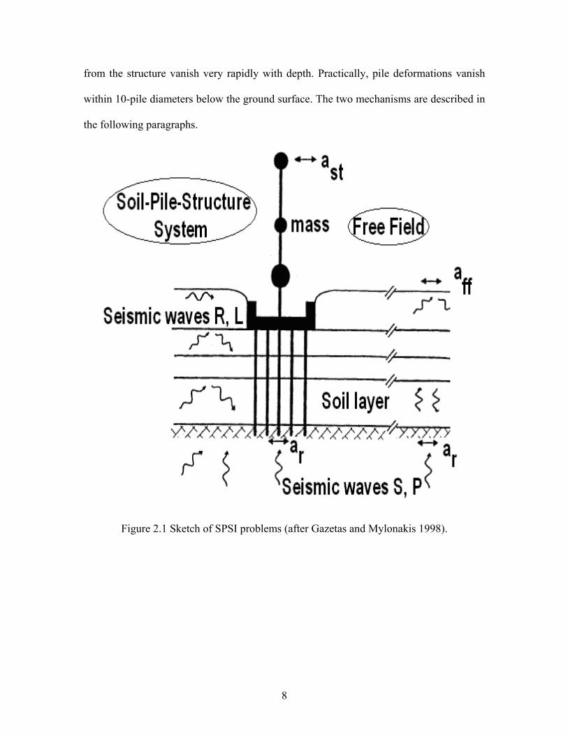
from the structure vanish very rapidly with depth. Practically, pile deformations vanish

within 10-pile diameters below the ground surface. The two mechanisms are described in

the following paragraphs.

Figure 2.1 Sketch of SPSI problems (after Gazetas and Mylonakis 1998).

8

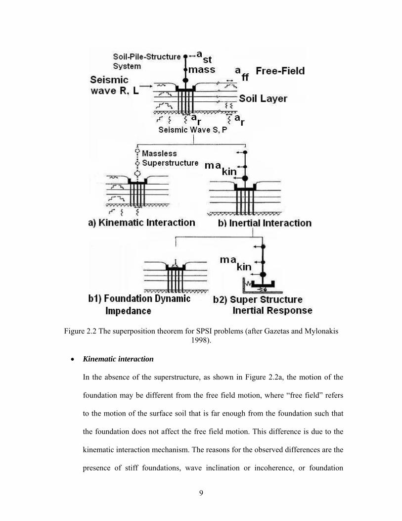
Figure 2.2 The superposition theorem for SPSI problems (after Gazetas and Mylonakis 1998).

• Kinematic interaction

In the absence of the superstructure, as shown in Figure 2.2a, the motion of the

foundation may be different from the free field motion, where “free field” refers

to the motion of the surface soil that is far enough from the foundation such that

the foundation does not affect the free field motion. This difference is due to the

kinematic interaction mechanism. The reasons for the observed differences are the

presence of stiff foundations, wave inclination or incoherence, or foundation

9

embedment. Kinematic effects are described by frequency dependent transfer

functions. The transfer function is defined by the ratio of the foundation motion to

the free field motion in the absence of a structure. Transfer functions are defined

in the frequency domain. Wave passage through the foundation also generates

stress in foundation elements. These stresses are termed “kinematic stresses”.

• Inertial interaction

The motion at the foundation due to kinematic interaction forces the structure to

oscillate. This, in turn, implies that the structure will produce inertial forces and

overturning moments at its base. Due to this, the foundation and surrounding soil

will get additional dynamic forces and displacements. This is due to the inertial

interaction. The flexibility of the foundation support affects the acceleration

within the structure. The flexibility of the foundation and the damping associated

with foundation-soil interaction can be described by a frequency dependent

foundation impedance function (dynamic impedance). The dynamic impedance

can be simulated by the effects of a “spring” and a “dashpot” acting at the base of

the structure in place of the foundation elements.

The above two mechanisms occur simultaneously with only a small time lag. In the two-

step approach, the acceleration at the top of the foundation is obtained by modifying the

free field motion to account for kinematic effects. This motion, akin, is then used as an

input motion for the analysis of inertial interaction. For computational convenience, the

analysis of inertial interaction is further subdivided into two steps, as shown in Figures

2.2 b1 and 2.2 b2. First, a dynamic impedance function at the top of the foundation is

10

computed for the pile-soil system. As a final step, the superstructure, supported on the

spring and dashpot system is analyzed using akin as the input motion.

Typically, structural design engineers neglect the kinematic interaction. This is

acceptable in some circumstances such as at low frequencies (Mamoon and Ahmad 1990)

and for shallow foundations with vertically propagating shear waves or dilatational

waves. However, Gazetas (1984) carried out analysis on flexible piles with low frequency

loading and concluded that kinematic interaction is also important. In almost every

seismic building code, structural response and foundation loads are computed by fixed

base analysis; that is, SPSI is neglected.

Eurocode 8 (Eurocode 8-part 5 1999) acknowledges the potential effect of SPSI

and suggested that SPSI should be considered for the following cases:

• “Structures where p-δ effects play a significant role;

• Structures with massive or deep seated foundations;

• Slender tall structures;

• Structures supported on very soft soils, with average shear wave velocity less than

100 m/s.”

Furthermore, Eurocode 8 suggested that kinematic interaction should be considered only

when two or more of the following conditions happen simultaneously:

• “The subsoil profile is of class C (soft soil), or worse, and contains consecutive

layers with sharply differing stiffness;

• The zone is of moderate or high seismicity, α > 0.1 [where α is the expected

PGA];

• The supported structure is of importance category I or II.”

11

Kim and Stewart (2003) used 29 earthquake strong motion recordings from sites

where there was a recording on a structure and a recording on the free-field to evaluate

differences between foundation level and free field level ground motions. That is, they

found the empirical frequency dependent transfer function amplitude. Kim and Stewart

(2003) developed procedures to fit transfer function amplitude to analytical models for

base slab averaging. The above procedures were developed with the assumed conditions

of a rigid base slab and a vertically propagating, incoherent incident wave field

characterized by ground motion incoherence parameter, k.

2.2.2 Numerical tools

Several methods have been used in the past to study the SPSI problem. These

include numerical methods such as the FEM, boundary element methods, and Beam on

Winkler Foundation models, Semi empirical and Semi analytical methods, and analytical

solutions have also been developed. Penzien (1970) was the first to successfully use a

Beam on Winkler foundation model for dynamic analysis. This type of model has been

used extensively since. Boundary element formulations for seismic loading were

developed by Poulos (1968, 1971), Butterfield & Banerjee (1971), Kausel & Peek (1982),

Kaynia & Kausel (1982), Sen et al. (1985), and Ahmad & Mamoon (1991). Boundary

element solutions cannot incorporate nonlinear soil behavior or soil-pile interface

behavior. However, this method offers a good solution for problems involving a variety

of incident wave fields such as vertical and inclined body waves and Rayleigh waves.

Given that the focus of this study is numerical modeling of SPSI using the FEM, the

literature review presented in the next section focuses on the FEM as applied to SPSI

problems.

12

2.3 FINITE ELEMENT METHOD APPLIED TO SPSI PROBLEMS

The FEM is a useful tool in the analysis of boundary value problems for any

continuous medium. There are numerous problems in solid mechanics where the FEM is

the only easy tool for the analysis. For example in the area of plasticity, performing

nonlinear analysis by means of analytical or semi analytical formulations is tedious,

especially for complicated geometries such as a pile in layered soil. Such nonlinear

analyses can be solved with the finite element method to a much easier extent. Seismic

loading problems can also be solved using the FEM. The above phenomena are usually

encountered in geotechnical applications.

The literature on the FEM and on applications of the FEM to geotechnical

engineering is extensive. The literature review presented herein focuses on the use of the

FEM to solve SPSI problems under dynamic conditions. The general treatment of the

various elements of an FEM solution (e.g. boundary conditions, load application, etc) in

SPSI problems is presented first, followed by a thorough review of previous work on the

use of FEM to solve specific dynamic SPSI problems.

2.3.1 Boundary conditions

The use of FEA for dynamic analyses differs from static analyses in considering

the soil strata as infinite in the horizontal direction (and sometimes in the vertical

direction as well). In FEA the structures underneath the soil surface are generally

assumed to be surrounded by infinite soil medium, while structures on and near the soil

surface are assumed to lie on a semi infinite half space. In static analyses, fixed boundary

conditions can be applied at some distance from the region of interest. In dynamic

problems, however, such boundary conditions will reflect outward propagating waves

13

back into the model. Furthermore, fixed boundary conditions do not model adequately the

outward radiation of energy at the boundaries of the model. A larger model can minimize

this problem because material damping will absorb most of the energy in the waves

reflected from finite boundaries. However, the increase in model size implies an

unwanted, and probably excessive, increase in computational time. Furthermore,

symmetric and anti- symmetric geometries in boundary value problems can be used to

reduce the FEA time. Examples of both cases are found in Bentlet and Naggar (2000),

where the authors took advantage of symmetry by restricting horizontal displacements

perpendicular to the symmetric axis; and in Maheshwari et al. (2004), where the authors

took advantage of the symmetry as well as the anti-symmetry.

There are three alternative methods available in finite element programs to

appropriately model the infinite medium boundary conditions. These methods are

reviewed in the following paragraphs.

Kelvin element

Kelvin elements can be attached to a boundary in order to simulate an infinite

medium. A Kelvin element consists of a spring and a dashpot attached in parallel. The

spring provides stiffness necessary to keep the static load in equilibrium. The viscous

dashpot absorbs the energy that reaches the boundary. Dashpot and spring coefficients

can be determined using the solution developed by Novak and Mitwally (1988). This

element is usually used to simulate the boundaries involved in both static and dynamic

analyses. In static analyses, the damping term vanishes because of its dependency on

frequency: since a dashpot absorbs energy as a function of velocity, when the velocity is

zero, the dashpot force is also zero. Bentlet and Naggar (2000) and Maheshwari et al.

14

(2004) used Kelvin elements in their analysis of SPSI for single and group pile

foundations.

Viscous element (dashpot element)

Viscous elements proposed originally by Lysmer and Kuhlemeyer (1969) for

shallow foundations are used when the simulation has only dynamic loading (e.g. the

zero frequency component of loading is zero). The dashpots absorb energy reaching the

boundary. The Dashpot coefficient per unit area in the directions perpendicular and

tangential directions to the boundary can be calculated from the following equation:

pSn VC ρ= and SSt VC ρ= (2.1)

where, Sρ is density of the soil, is p wave velocity, is shear wave velocity, is

coefficient per unit area perpendicular to boundary, and is coefficient per unit area

tangent to boundary. Viscous dashpots are used often in site response and SPSI problems

(e.g., Rodriguez-Marek and Bray 2005, Borja et al. 2002, Wu and Finn 1997, among

others).

pV SV nC

tC

Infinite elements

Infinite elements are used in boundary value problems with unbounded

boundaries (infinite medium) or in problems with a smaller region of interest compared

to the surrounding medium. Infinite elements are usually used in conjunction with finite

elements. The behavior of the infinite element is similar to the behavior of the Kelvin

element, but far nodes are not allowed to move. An infinite element behaves linearly.

During static analyses, infinite elements will provide stiffness at the finite element model

boundaries based on the model of Zienkiewicz et al. (1983). During the dynamic

analysis, infinite elements will provide “quiet” boundaries at the finite element model

15

boundaries based on the model of Lysmer and Kuhlemeyer (1969) (ABAQUS 2005). The

dynamic response of the infinite elements is based on consideration of plane body waves

traveling orthogonally to the boundary. Again, it is assumed that the response adjacent to

the boundary is of small enough amplitude so that the medium responds in a linear elastic

fashion. An example of the application of infinite elements in dynamic problems is the

wave propagation analysis of Zhao and Valliappan (1993).

2.3.2 Soil-pile interface

Soil-pile interface modeling also contributes to the behavior of the soil-pile-

structure system. The soil-pile interfaces are usually modeled in two ways, either as a

perfectly bonded interface or as a frictional interface where soil-pile slipping and gapping

may occur. In reality, the interface should be modeled to incorporate slipping and

gapping. However, computational time and modeling difficulties lead researchers to

consider perfect bonding in some applications and if the problem to be analyzed is not

dependent on slipping and gapping, this solution may suffice. Generally, Coulomb’s law

of friction is used to model slipping and gapping in FEA. If the interface surface is in

contact, full transfer of shear stress is ensured. Plastic slipping will occur, when the

friction stress exceeds the minimum of a user specified maximum shear stress or the

friction stress due to the normal stresses at the surface (µp). Separation will occur when

there is tension between the soil and pile interface. Besides the Coulomb friction model,

there are other proposed interface models available in the literature (e.g., Desai et al.

1984 and 1985, Desai and Nagaraj 1986, Drumm 1983, Drum and Desai 1986, Ghaboussi

et al. 1973, Goodman et al. 1968, Herrmann 1978, Idriss et al. 1979, Isenberg and

16

Vaughan 1981, Katona 1981, Kausel and Roesset 1974, Roesset and Scarletti 1979, Toki

et al. 1981, Vaughan and Isenberg 1983, Wolf 1985, and Zaman et al. 1984).

2.3.3 Loading

In a typical seismic analysis using FE, the seismic load can be applied either at the

base, as a displacement or acceleration time history, or as a force per unit volume (f=-

abaseρ, where ρ is density of the soil and abase is acceleration at base) distributed

throughout the mesh.

2.3.4 Soil behavior

Soil-Pile interaction behavior also depends on the constitutive behavior of soil

model. Therefore, selection of a proper constitutive model leads to better results in FE

analysis. Constitutive models are widely used in numerical analysis of geomaterials.

They can be modeled to behave linear elastically, nonlinear elastically or

elsastoplastically. Hardening rules can be used to model elastoplastic behavior. The

Duncan-Chang model, which is widely used to model earth dams, is a nonlinear elastic

model (Duncan and Chang 1970). An elastoplastic constitutive model can provide a

better representation for a typical wave propagation problem (Prevost 1977, Bardet 1989,

Dafalias 1986, Finn 1988). Some of the constitutive models are readily available in finite

element programs. New constitutive models can be incorporated in finite element

analysis programs by user-defined subroutines.

2.3.5 Applications

This study focuses only on FEM; hence, in the following text a brief review on

published studies of seismic SPSI problems using FEM is summarized.

17

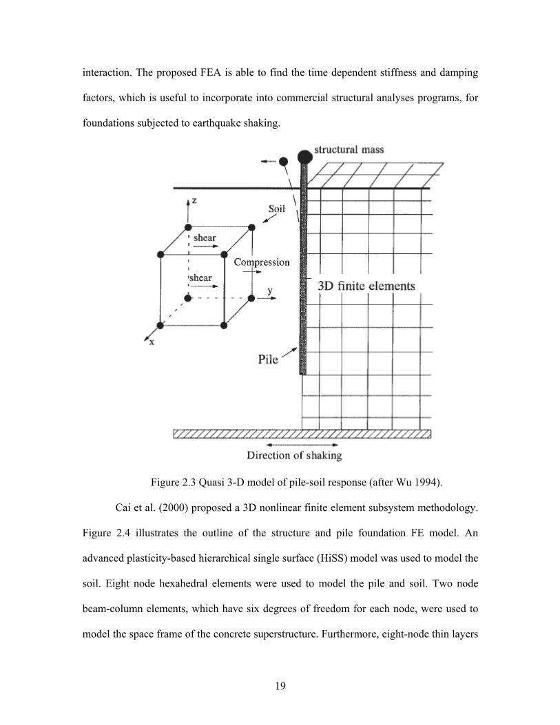
A quasi 3-D finite element method was proposed for dynamic elastic and

nonlinear analysis of pile-soil-structure interaction by Wu and Finn (1997). The principle

of the quasi 3-D model is shown in Figure 2.3 (Wu 1994, Finn et al. 1997, Wu and Finn

1997). This model was developed under the following assumptions. First, shear waves in

the XY and YZ planes governed the dynamic motions, and the compression waves in the

shaking direction, Y (refer the Figure 2.3). Second, deformations were neglected in the

vertical direction and normal to the direction of shaking. Dashpots were used to simulate

the infinite soil medium. The model was validated with centrifuge tests performed by

Gohl (1991) at the California Institute of Technology (Caltech) on a single pile and a 2 x

2 pile group. 8-node brick elements were used to represent the soil and 2-node beam

elements were used to represent the pile. Displacement compatibility between soil to pile

is enforced. This model incorporated soil yielding and gapping between the pile and

attached soil. An equivalent linear method was used to model the nonlinear hysteretic

behavior of soil. That is, instead of varying the shear modulus with strain, a single

effective value was used for the entire time history. In the single pile model, the

superstructure mass was a rigid body and its motion was represented by a concentrated

mass at its center of gravity. A very stiff beam element with flexural rigidity 1000 times

that of the pile was used to connect the superstructure and pile. Symmetric boundary

conditions were used. In the group pile model, a concentrated mass at the center of

gravity of the pile cap represented the rigid pile cap and mass-less rigid bars were used to

connect the piles. The mass and pile heads were connected by very stiff mass-less beam

elements. The results of the FEA showed that stiffness of the pile foundation decreases

with the level of shaking. The analysis also showed the importance of the inertial

18

interaction. The proposed FEA is able to find the time dependent stiffness and damping

factors, which is useful to incorporate into commercial structural analyses programs, for

foundations subjected to earthquake shaking.

Figure 2.3 Quasi 3-D model of pile-soil response (after Wu 1994).

Cai et al. (2000) proposed a 3D nonlinear finite element subsystem methodology.

Figure 2.4 illustrates the outline of the structure and pile foundation FE model. An

advanced plasticity-based hierarchical single surface (HiSS) model was used to model the

soil. Eight node hexahedral elements were used to model the pile and soil. Two node

beam-column elements, which have six degrees of freedom for each node, were used to

model the space frame of the concrete superstructure. Furthermore, eight-node thin layers

19

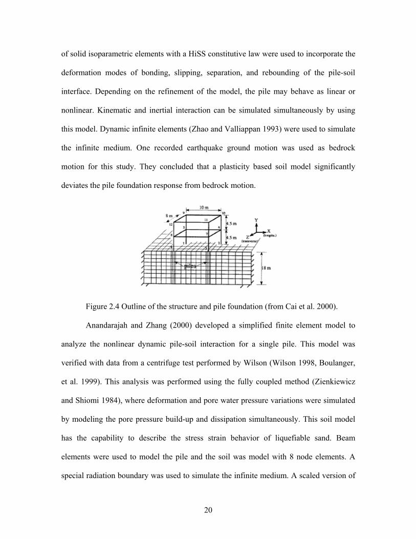
of solid isoparametric elements with a HiSS constitutive law were used to incorporate the

deformation modes of bonding, slipping, separation, and rebounding of the pile-soil

interface. Depending on the refinement of the model, the pile may behave as linear or

nonlinear. Kinematic and inertial interaction can be simulated simultaneously by using

this model. Dynamic infinite elements (Zhao and Valliappan 1993) were used to simulate

the infinite medium. One recorded earthquake ground motion was used as bedrock

motion for this study. They concluded that a plasticity based soil model significantly

deviates the pile foundation response from bedrock motion.

Figure 2.4 Outline of the structure and pile foundation (from Cai et al. 2000).

Anandarajah and Zhang (2000) developed a simplified finite element model to

analyze the nonlinear dynamic pile-soil interaction for a single pile. This model was

verified with data from a centrifuge test performed by Wilson (Wilson 1998, Boulanger,

et al. 1999). This analysis was performed using the fully coupled method (Zienkiewicz

and Shiomi 1984), where deformation and pore water pressure variations were simulated

by modeling the pore pressure build-up and dissipation simultaneously. This soil model

has the capability to describe the stress strain behavior of liquefiable sand. Beam

elements were used to model the pile and the soil was model with 8 node elements. A

special radiation boundary was used to simulate the infinite medium. A scaled version of

20

a recording from the Kobe event (Event J) was considered as an input motion. Results

from the FEA and the centrifuge tests agree well.

Kishishita et al. (2000) performed linear and nonlinear analysis by using 2D finite

element analysis for friction type micropiles. The soil was modeled with two layers. In a

linear analysis, three models were developed with varying shear wave velocity for the

upper layer while the shear wave velocity for the lower layer was constant in all cases.

Furthermore, four different type of pile foundations (pre-cast piles, cast-in-situ piles,

high-capacity micropiles, and high-capacity micropiles for raked piles) were examined.

The El Centro motion from the 1940 earthquake of the same name and the K.P-83 motion

from the 1995 Kobe earthquake were used as input motions. The softest soil was

considered in nonlinear analysis because generally piles are used in the softest soil. Soil

was modeled with the modified Ramberg-Osgood model. Cast-in-situ piles, pre-cast piles

and high capacity micropiles were modeled with tri-linear, modified Takeda, and bilinear

models, respectively. From their work it was found that the horizontal response of the

footing was almost the same regardless of the pile type because it is controlled by soil

response. For soft soils, the piles had the largest influence in both vertical and horizontal

response of the footing, in particular when the piles were raked.

Brown et al. (2001) and Bentley and Naggar (2000) studied the effects of

kinematic interaction on the input motion at the foundation level. In this study they

incorporated pile-soil separation, slippage, soil plasticity, and 3D wave propagation. The

FE analysis was carried out using the FE program ANSYS (ANSYS Inc. 1996). By

considering symmetry, one half of the actual model was developed in order to reduce the

computing time. Kelvin elements were used to simulate the infinite soil medium. Soil

21

was modeled as a linear and an elastoplastic material using the Drucker-Prager failure

criterion. Linear elastic cylindrical piles were considered for this study. Two different

type of pile-soil interfaces were considered: the pile-soil interface was either perfectly

bonded or a frictional interface was used between pile and soil surfaces. A Coulomb

frictional model was used to incorporate the above behavior. Floating and socketed

(fixed-end) piles were modeled in the analysis. Two recorded strong-motions were used

in this study. Brown et al. (2001) and Bentley and Naggar (2000) concluded in their

studies that elastic kinematic interaction for a single pile slightly amplifies the free field

transfer function (e.g., the ratio of soil to bedrock motion). Overall, the kinematic

interaction response is equivalent to free field response for the assumptions made in their

study.

Shahrour et al. (2001) performed a 3-D finite element analysis for micropiles

(small diameter piles). The FEA results were compared with those of a simplified model

based on the Beam on Winkler foundation approach. In this study, seismic behavior of a

single micropile and a micropile group supporting a superstructure were considered. A

single degree of freedom structure composed of a concentrated mass and a column was

used to model the superstructure. In the group micropile analysis, three cases were

considered: a group composed of three micropiles in a row alignment (1 x 3), a square

group including 9 elements (3 x 3), and a group of 15 micropiles (3 x 5). In this analysis,

square cross section micropiles embedded in a homogenous soil layer underlain by rigid

bedrock were considered. The behavior of the soil-micropile-structure system was

assumed to be elastic with Rayleigh material damping. Furthermore, the following

boundary conditions were imposed in this simulation: the base was fixed, periodic

22

conditions were imposed at lateral boundaries for the displacement field, and harmonic

acceleration (ag=0.2 g, f=0.67 Hz) was applied at the base of the soil. The study showed

that the inertial effect is mostly seen on the upper part of the micropiles. Inertial effect

mainly depends on mass and frequency of the superstructure. In the group pile analysis,

seismic loading is not distributed uniformly in the micropiles. A group effect was also

observed due to inertial forces in this study.

Ousta and Shahrour (2001) performed a 3-D finite element analysis in order to

study the seismic behavior of micropiles used for reinforcement of saturated sand. The

analysis was carried out using the (u-p) formulation (displacement for the solid phase and

pore-pressure for the fluid phase) proposed by Zienkiewicz et al. (1980). A soil model

based on the bounding surface concepts was used and kinematic and isotropic hardening

were used to capture the elasto-plastic behavior. A single micropile and micropile groups

(2x2, 3x3) were modeled in this analysis. Micropiles were modeled with a linear elastic

model. The interface between soil and pile was assumed as perfect bonding. The analysis

was carried out under the following boundary conditions: the base of the soil was fixed

and impervious, the water table was assumed to be at the ground surface, and periodic

conditions were applied at lateral boundaries for both pore-pressure and displacements. A

harmonic acceleration (ag=0.1 g, f=2 Hz) was considered as an input motion at the base.

The analyses for micro piles under loose to medium sand showed that seismic loading

induces an increase in the pore-pressure, which leads to an increase in the bending

moment of the micropile. However, group effects reduce the bending moment

significantly.

23

Sadek and Shahrour (2003) studied the influence of pile inclination on seismic

behavior of micropile groups by using a 3-D finite element analysis. The structure

represented by a concentrated mass and a column was modeled with a single degree of

freedom. Soil was modeled elastically with Rayleigh damping and the piles were

modeled with 3D elastic beam elements. A pile cap, which was free of contact with the

soil, was used to connect the piles. 2x2 micropile groups with different inclinations (0°,

7°, 13°, 20°) with vertical axis were considered in this analysis. A harmonic acceleration

(ag=0.2g, f=0.43Hz) was applied at the base as an input motion and Young’s modulus of

the soil, , was assumed to increase with depth, z, based on: )(zEs

5.0

)()( ⎥⎦

⎤⎢⎣

⎡=

asos p

zpEzE (2.2)

zK

zp so ρ⎥⎦

⎤⎢⎣⎡ +

=3

)21()( i )f ()(, oo zpzpzz == (2.3)

where, is the mean stress due to the self-weight of the soil at the depth , is a

reference pressure of 100 kPa, is the Young’s modulus of soil when , is the

coefficient of lateral earth pressure at rest, and is the thickness of the soil layer that is

closest to the surface with constant Young’s modulus. Results showed that inclination of

the micropiles increase their lateral stiffness.

)z(p z ap

soE app = oK

oz

Maheshwari et al. (2004) developed a 3-D finite element model to examine the

effects of soil plasticity (including work hardening) and separation at the soil-pile

interface on the dynamic response of a single pile and pile groups. The pile was modeled

with a linear elastic material and the soil was modeled with an advanced plasticity-based,

hierarchical single surface (HISS) model. Only one fourth of the model was constructed

24

by considering symmetry and anti symmetry. Kelvin elements (spring and dashpot) were

used in all three directions (i.e., X, Y and Z) to simulate the infinite soil medium. The

model was loaded (at the base, which is assumed to represent bed rock) with the El

Centro (north-south component) acceleration record from the 1940 El Centro Earthquake.

Furthermore, harmonic motion was used to find the transfer and impedance functions for

the foundation. Pile-soil separation was considered only in the loading direction while the

pile and soil were assumed to be in contact in the direction perpendicular to the motion.

Friction between pile and soil were neglected. In every Gaussian point normal stress in

soil elements (in the direction of loading) and confining pressure at that depth were

compared for every time step and at every iteration within a time step. Separation was

assumed when tensile normal stress was higher than confining stress.

Numerical analyses by Maheshwari et al. (2004) reveal that the effect of

separation was more significant when using the elastic soil model rather than the plastic

model. Also, nonlinearity reduced the real and imaginary part of the impedance function

for the pile system. Moreover, soil nonlinear response in the soil-pile system has

significant effect for low excitation frequencies.

2.4 p-y CURVES

Design engineers often prefer to use the Beam-on-Dynamic-Winkler-Foundation

(BDWF) model for design purposes rather than the FE method or elastic continuum

solutions. BDWF methods use traditional semi empirical p-y curves such as those

developed by Matlock (1970) and Reese et al. (1974). These curves represent the

nonlinear soil behavior by a series of nonlinear springs, where the p refers to soil pressure

per unit length of pile and the y refers to deflection. The loading in the pile is traditionally

25

applied as a factored static load at the pile-top. This review focuses on p-y curves

developed within this approach, that is, obtained from static tests. It is important to note,

however, that pseudo-static loading may be correct for low frequency vibration design,

but response may change significantly when seismic loading generates the introduction of

soil nonlinearity, damping, and pile-soil interaction. Other authors (Naggar and Novak

1996, Brown et al. 2001) have developed p-y methods that can deal with dynamic

loading.

Most of the existing standard p-y curves were developed based on full-scale

lateral load tests on a relatively small range of pile diameters. However, Juirnarongrit

(2002) showed that in dense weakly cemented sand, the pile diameter effect on the p-y

curves at displacement levels below the ultimate soil resistance is insignificant. Beyond

this range, an increment in the pile diameter increases the ultimate soil resistance.

Existing p-y curves predict the response of the laterally loaded piles well in weakly

cemented sand but are inappropriate for large diameter piles. These existing p-y curves

have been incorporated into commercial programs such as COM624P (Wang and Reese

1993), LPILE (Reese et al. 2000), and FLPIER (University of Florida 1996). Deflection

and moment along the pile can be found for a given load by using these commercial

programs. The literature review presented herein focuses on the existing p-y curves for

laterally loaded piles and methods to find p-y curves from numerical analysis. Existing

p-y curves for clay and sand are presented first, and then the effect of diameter in p-y

curves are discussed followed by a thorough review of back calculation of p-y curves

from numerical analysis.

26

2.4.1 Existing p-y curves

Figure 2.5 graphically shows the concept of a p-y curve. The pile is assumed to be

perfectly straight prior to loading (i.e. there was no bending during pile driving). Prior to

loading, the soil pressure acting against the pile can be assumed to be uniform across its

diameter (see Figure 2.5), implying that the resultant horizontal pressure acting against

the pile is zero. During loading the resultant force per meter length of pile can be found

by integration of the soil pressure around the pile. This process can be continued for a

series of deflections that would give series of forces per unit length of pile, which will

produce a p-y curve. In a similar manner, the sets of p-y curves along the pile can be

obtained (refer Figure 2.6).

Figure 2.5 Definition of p-y concept with a) Pile at rest: b) Pile after load applied (after Dunnavant 1986).

27

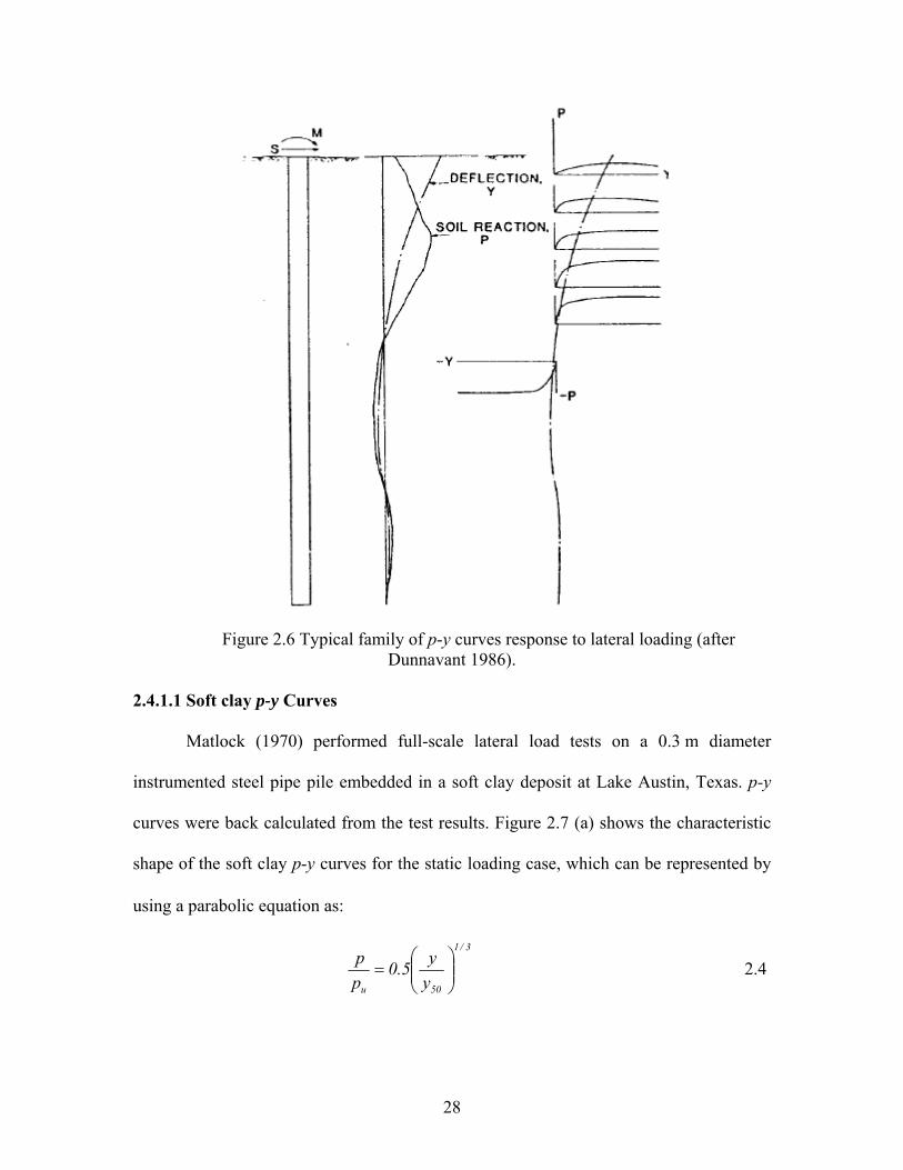
Figure 2.6 Typical family of p-y curves response to lateral loading (after Dunnavant 1986).

2.4.1.1 Soft clay p-y Curves

Matlock (1970) performed full-scale lateral load tests on a 0.3 m diameter

instrumented steel pipe pile embedded in a soft clay deposit at Lake Austin, Texas. p-y

curves were back calculated from the test results. Figure 2.7 (a) shows the characteristic

shape of the soft clay p-y curves for the static loading case, which can be represented by

using a parabolic equation as:

3/1

50u yy5.0

pp

⎟⎟⎠

⎞⎜⎜⎝

⎛= 2.4

28

where, pu is the ultimate soil resistance which is related to undrained shear strength of the

soil as well as being a function of depth and y50: the soil displacement at one-half of

ultimate soil resistance.

Figure 2.7(b) shows the characteristic shape of the soft clay p-y curves for the

cyclic loading case. The main difference between static and cyclic loading is that the soil

resistance for cyclic loading at large strain levels is decreased. The methodology to

develop p-y curves for static and cyclic loading is given in Table 2.1.

Figure 2.7 Characteristic shape of p-y curve for soft clay a) Static loading: b) Cyclic loading (after Matlock 1970).

2.4.1.2 Stiff clay p-y curves below the water table

Reese et al. (1975) conducted a lateral load test on two 0.6 m diameter driven

steel pipe piles embedded in stiff clay under the water table at Manor, Texas. Figure 2.8

shows the characteristic shape of p-y curves for both static and cyclic loading. The soil

resistance at larger strains for both cases is lower than the peak resistance. The same

parameters used in the soft clay p-y curves are used to describe the characteristic shape of

the stiff clay p-y curves. The methodology to develop p-y curves for static and cyclic

loading is given in Table 2.2.

29

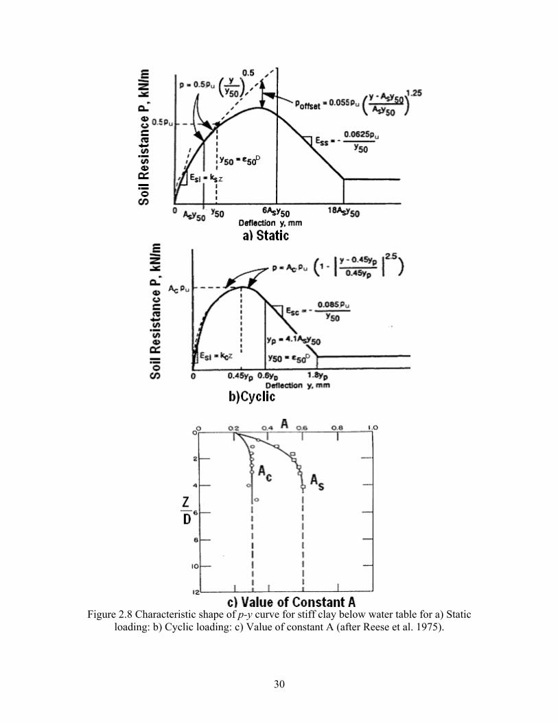
Figure 2.8 Characteristic shape of p-y curve for stiff clay below water table for a) Static

loading: b) Cyclic loading: c) Value of constant A (after Reese et al. 1975).

30

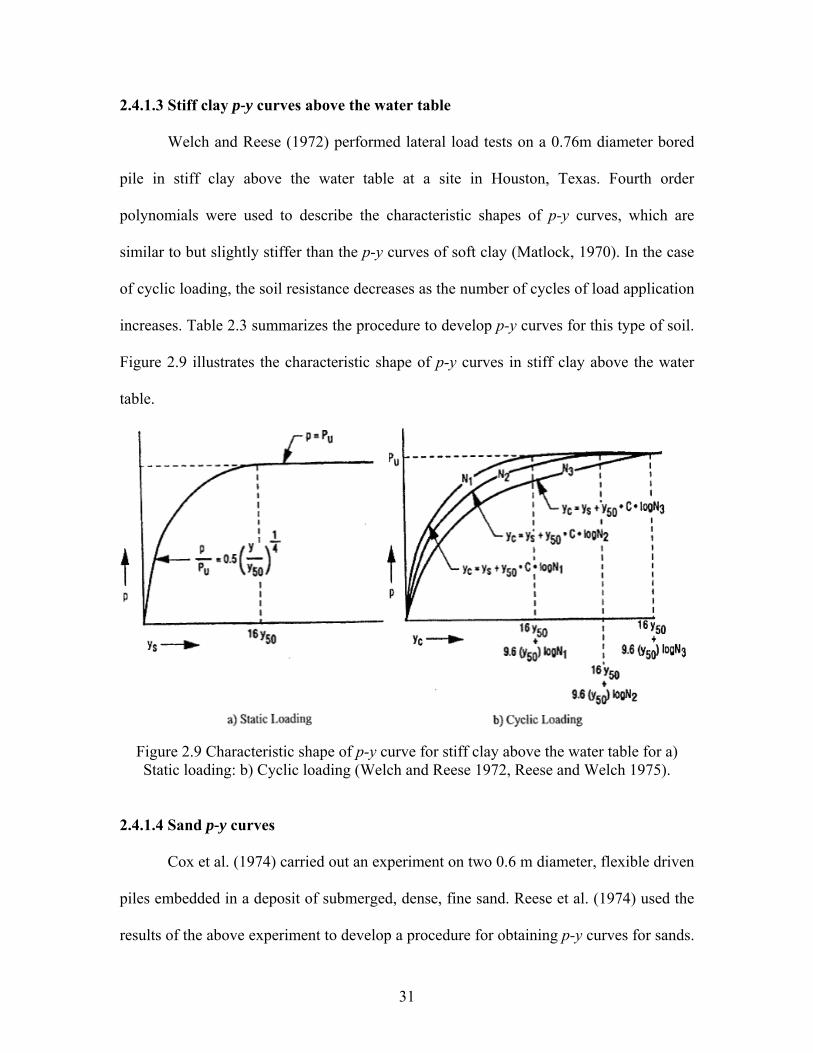
2.4.1.3 Stiff clay p-y curves above the water table

Welch and Reese (1972) performed lateral load tests on a 0.76m diameter bored

pile in stiff clay above the water table at a site in Houston, Texas. Fourth order

polynomials were used to describe the characteristic shapes of p-y curves, which are

similar to but slightly stiffer than the p-y curves of soft clay (Matlock, 1970). In the case

of cyclic loading, the soil resistance decreases as the number of cycles of load application

increases. Table 2.3 summarizes the procedure to develop p-y curves for this type of soil.

Figure 2.9 illustrates the characteristic shape of p-y curves in stiff clay above the water

table.

Figure 2.9 Characteristic shape of p-y curve for stiff clay above the water table for a) Static loading: b) Cyclic loading (Welch and Reese 1972, Reese and Welch 1975).

2.4.1.4 Sand p-y curves

Cox et al. (1974) carried out an experiment on two 0.6 m diameter, flexible driven

piles embedded in a deposit of submerged, dense, fine sand. Reese et al. (1974) used the

results of the above experiment to develop a procedure for obtaining p-y curves for sands.

31

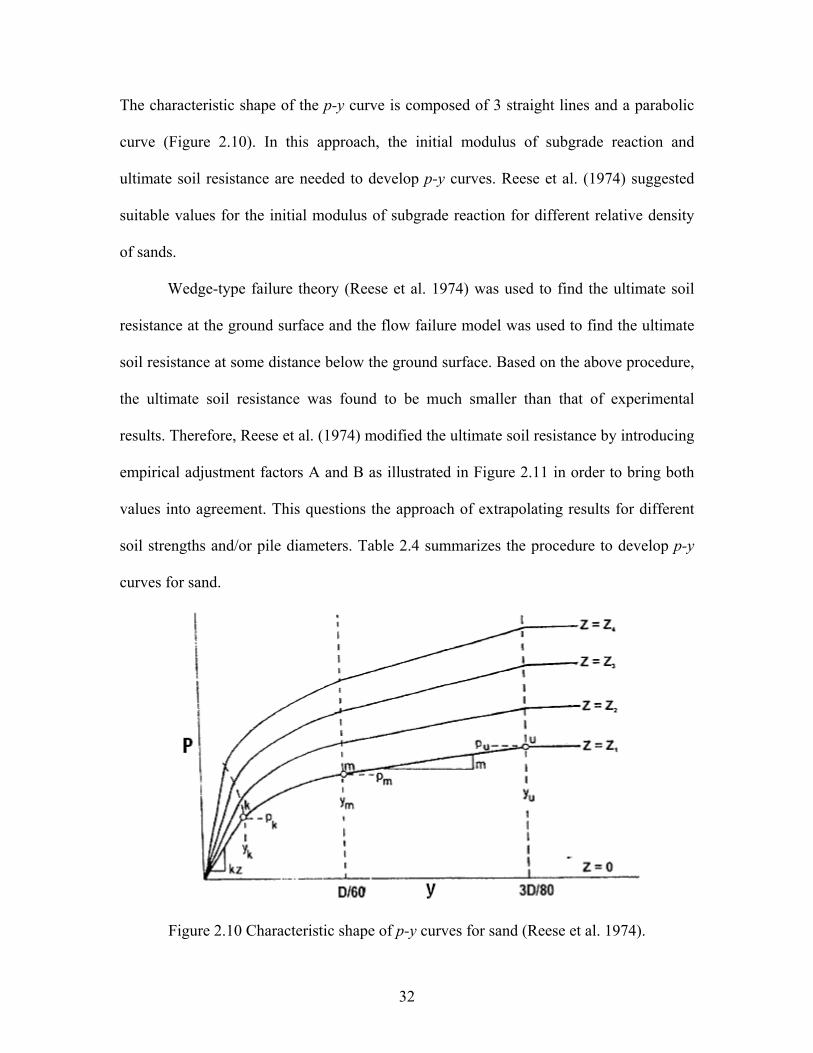
The characteristic shape of the p-y curve is composed of 3 straight lines and a parabolic

curve (Figure 2.10). In this approach, the initial modulus of subgrade reaction and

ultimate soil resistance are needed to develop p-y curves. Reese et al. (1974) suggested

suitable values for the initial modulus of subgrade reaction for different relative density

of sands.

Wedge-type failure theory (Reese et al. 1974) was used to find the ultimate soil

resistance at the ground surface and the flow failure model was used to find the ultimate

soil resistance at some distance below the ground surface. Based on the above procedure,

the ultimate soil resistance was found to be much smaller than that of experimental

results. Therefore, Reese et al. (1974) modified the ultimate soil resistance by introducing

empirical adjustment factors A and B as illustrated in Figure 2.11 in order to bring both

values into agreement. This questions the approach of extrapolating results for different

soil strengths and/or pile diameters. Table 2.4 summarizes the procedure to develop p-y

curves for sand.

Figure 2.10 Characteristic shape of p-y curves for sand (Reese et al. 1974).

32

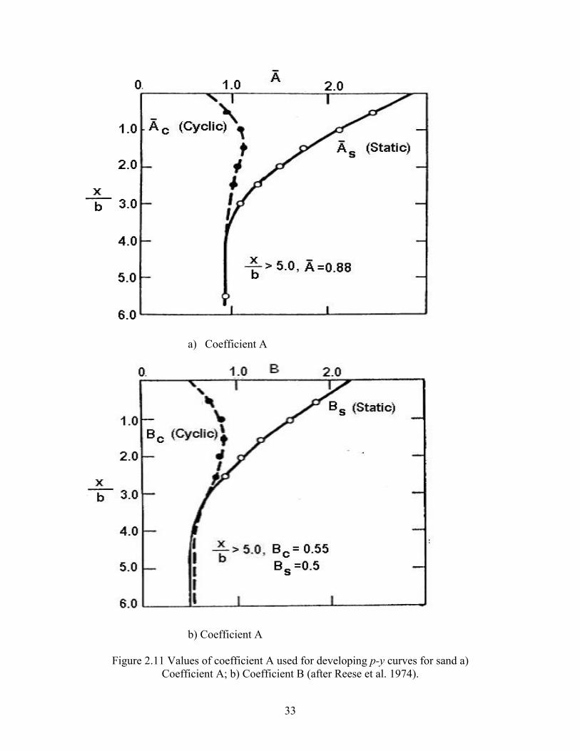
a) Coefficient A

b) Coefficient A

Figure 2.11 Values of coefficient A used for developing p-y curves for sand a) Coefficient A; b) Coefficient B (after Reese et al. 1974).

33

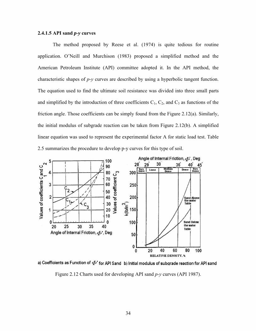
2.4.1.5 API sand p-y curves

The method proposed by Reese et al. (1974) is quite tedious for routine

application. O’Neill and Murchison (1983) proposed a simplified method and the

American Petroleum Institute (API) committee adopted it. In the API method, the

characteristic shapes of p-y curves are described by using a hyperbolic tangent function.

The equation used to find the ultimate soil resistance was divided into three small parts

and simplified by the introduction of three coefficients C1, C2, and C3 as functions of the

friction angle. Those coefficients can be simply found from the Figure 2.12(a). Similarly,

the initial modulus of subgrade reaction can be taken from Figure 2.12(b). A simplified

linear equation was used to represent the experimental factor A for static load test. Table

2.5 summarizes the procedure to develop p-y curves for this type of soil.

Figure 2.12 Charts used for developing API sand p-y curves (API 1987).

34

2.4.1.6 p-y curves for φ−c soils

Using the traditional Mohr-Coulomb simplification of a linear failure envelope in

the shear stress vs. normal stress plane, soils can be classified either as cohesive or

cohesionless. Based on the above classification, theories were developed to analyze

geotechnical problems of soil-pile interaction. This concept may lead to significantly

conservative design for cemented soil or silt because they always neglect the soil

resistance from the cohesion component.

Ismael (1990) performed full-scale lateral load pile test under static loading in

Kuwait. Tests were carried out for single piles and small pile groups embedded in

medium dense cemented sands. Tests were carried out using 0.3 m diameter reinforced

concrete bored piles with pile lengths of 3m and 5m. Bending moment was measured for

2 piles by using electric resistance strain gauges. Friction ( ) and cohesion (20kPa)

were found using drained triaxial tests. It was shown that calculated p-y curves based on

sand p-y curves developed by Reese et al. (1974) were significantly underestimated by

the experimental results because of the presence of the cohesion components. A different

procedure was then developed to deal with the cohesion component. Figure 2.13

illustrates the theoretical parabolic p-y curves for

o35

φ−c type soils. Table 2.6 summarizes

the procedure to develop p-y curves for φ−c type of soil.

35

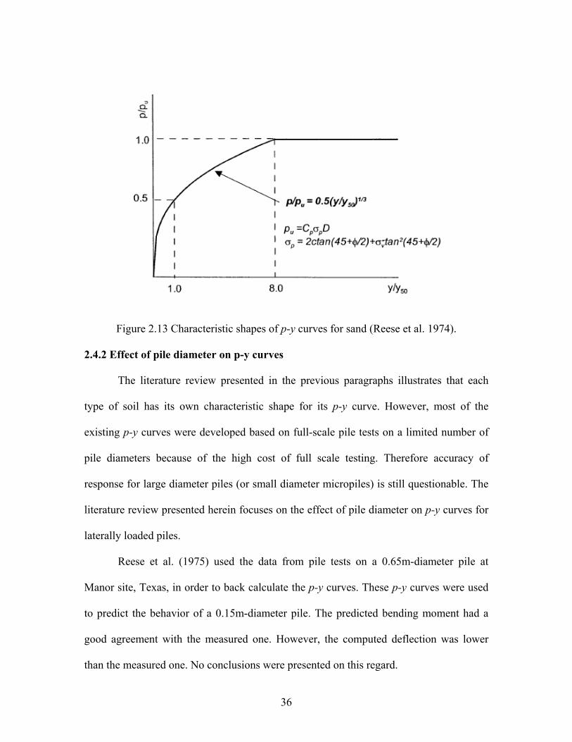
Figure 2.13 Characteristic shapes of p-y curves for sand (Reese et al. 1974).

2.4.2 Effect of pile diameter on p-y curves

The literature review presented in the previous paragraphs illustrates that each

type of soil has its own characteristic shape for its p-y curve. However, most of the

existing p-y curves were developed based on full-scale pile tests on a limited number of

pile diameters because of the high cost of full scale testing. Therefore accuracy of

response for large diameter piles (or small diameter micropiles) is still questionable. The

literature review presented herein focuses on the effect of pile diameter on p-y curves for

laterally loaded piles.

Reese et al. (1975) used the data from pile tests on a 0.65m-diameter pile at

Manor site, Texas, in order to back calculate the p-y curves. These p-y curves were used

to predict the behavior of a 0.15m-diameter pile. The predicted bending moment had a

good agreement with the measured one. However, the computed deflection was lower

than the measured one. No conclusions were presented on this regard.

36

O’Neill and Dunnavant (1984) and Dunnavant and O’Neill (1985) performed

laterally loaded pile tests on 0.27m, 1.22m, and 1.83m diameter piles embedded in

overconsolidated clay. They found that the deflection at one half of the ultimate soil

pressure (y50) is not linearly dependent on pile diameter. y50 reduces when the pile

diameter increases. That is, the pile diameter effect was not properly incorporated in the

clay p-y curves. A modification to Matlock’s p-y curves was proposed to match measured

p-y values.

Stevens and Audibert (1979) collected published case histories on laterally loaded

piles in clays. They used the existing p-y curves proposed by Matlock (1970) and API

(1987) in order to find the response of the piles. They found that the ratio between

computed to measured deflection was greater than one and increased with an increase of

pile diameter. However, computed maximum bending moments are higher than measured

values, in one case by as much as 30%. In order to force an agreement between both of

them, they suggested that y50 should be proportional to the square root of the pile

diameter. This also clearly indicates that existing p-y curves for soft clay do not

incorporate the effect of pile diameter.

2.4.3 Back calculation of p-y curves

FEA can be used to perform numerical tests and calculate p-y curves. p-y curves

can be back calculated using from FEA or full scale tests in two different methods. The

first method is by considering the bending moment along the pile. In this approach, an

analytical expression is fitted to the discrete moment data along the pile. The expression

is then differentiated twice in order to find the soil resistance p. The second method

consists of integrating the normal stress and shear stress applied on the pile by the soil

37

immediately surrounding it (Bransby 1999). Both methods can be used for static p-y

curves. However, the first method is difficult for dynamic p-y curves because it is

difficult to fit the analytical expression in each time increment.

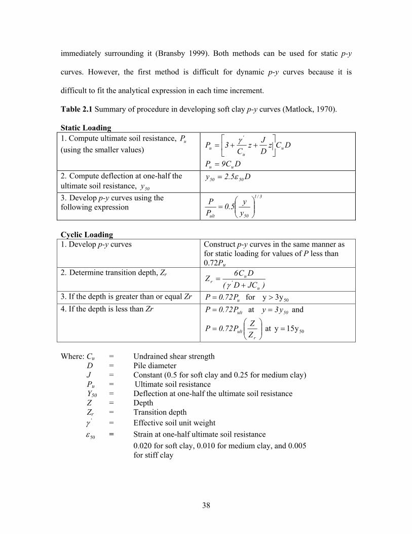
Table 2.1 Summary of procedure in developing soft clay p-y curves (Matlock, 1970). Static Loading 1. Compute ultimate soil resistance, uP

(using the smaller values) DCzDJz

C3P u

u

'

u ⎥⎦

⎤⎢⎣

⎡++=

γ

DC9P uu = 2. Compute deflection at one-half the ultimate soil resistance, 50y

D5.2y 5050 ε=

3. Develop p-y curves using the following expression

3/1

50ult yy5.0

PP

⎟⎟⎠

⎞⎜⎜⎝

⎛=

Cyclic Loading 1. Develop p-y curves Construct p-y curves in the same manner as

for static loading for values of P less than 0.72Pu

2. Determine transition depth, Zr

)JCD(DC6

Zu

'u

r +=

γ

3. If the depth is greater than or equal Zr uP72.0P = for 50y3y >4. If the depth is less than Zr ultP72.0P = at 50y3y = and

⎟⎟⎠

⎞⎜⎜⎝

⎛=

rult Z

ZP72.0P at 50y15y =

Where: Cu = Undrained shear strength D = Pile diameter J = Constant (0.5 for soft clay and 0.25 for medium clay) Pu = Ultimate soil resistance Y50 = Deflection at one-half the ultimate soil resistance Z = Depth Zr = Transition depth = Effective soil unit weight 'γ 50ε = Strain at one-half ultimate soil resistance 0.020 for soft clay, 0.010 for medium clay, and 0.005 for stiff clay

38

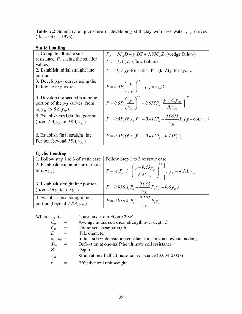
Table 2.2 Summary of procedure in developing stiff clay with free water p-y curves (Reese et al., 1975). Static Loading 1. Compute ultimate soil resistance, Pu (using the smaller values)

ZC83.2DZDC2P a'

aut ++= γ (wedge failure) DC11P uud = (flow failure)

2. Establish initial straight line portion

y)Zk(P s= for static, y)Zk(P c= for cyclic

3. Develop p-y curves using the following expression

5.0

50u y

yP5.0P ⎟⎟⎠

⎞⎜⎜⎝

⎛= , Dy 5050 ε=

4. Develop the second parabolic portion of the p-y curves (from

50s yA to ) 50s yA6

25.1

50s

50su

5.0

50u yA

yAyP055.0

yyP5.0P ⎟⎟

⎠

⎞⎜⎜⎝

⎛ −−⎟⎟

⎠

⎞⎜⎜⎝

⎛=

5. Establish straight line portion (from 50s yA6 to ) 50s yA18 )yA6y(P

y0625.0P411.0)A6(P5.0P 50su

50u

5.0su −−−=

6. Establish final straight line Portion (beyond ) 50s yA18

suu5.0

su AP75.0P411.0)A6(P5.0P −−=

Cyclic Loading 1. Follow step 1 to 3 of static case Follow Step 1 to 3 of static case 2. Establish parabolic portion (up to ) py6.0

⎥⎥

⎦

⎤

⎢⎢

⎣

⎡

⎟⎟⎠

⎞⎜⎜⎝

⎛ −−=

5.2

p

puc y45.0

y45.0y1PAP , 50cp yA1.4y =

3. Establish straight line portion (from to ) py6.0 py8.1 )y6.0y(P

y085.0PA936.0P pu

50uc −−=

4. Establish final straight line portion (beyond ) 50s yA8.1 pu

50uc yP

y102.0PA936.0P −=

Where: As, Ac = Constants (from Figure 2.8c) Ca = Average undrained shear strength over depth Z Cu = Undrained shear strength D = Pile diameter ks , kc = Initial subgrade reaction constant for static and cyclic loading Y50 = Deflection at one-half the ultimate soil resistance Z = Depth 50ε = Strain at one-half ultimate soil resistance (0.004-0.007) = Effective soil unit weight 'γ

39

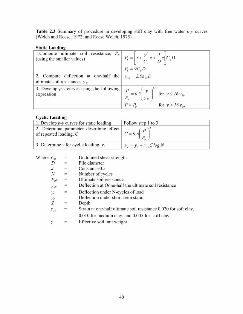
Table 2.3 Summary of procedure in developing stiff clay with free water p-y curves (Welch and Reese, 1972; and Reese Welch, 1975). Static Loading 1.Compute ultimate soil resistance, Pu (using the smaller values) DCz

DJz

C3P u

u

'

u ⎥⎦

⎤⎢⎣

⎡++=

γ

DC9P uu = 2. Compute deflection at one-half the ultimate soil resistance, 50y

D5.2y 5050 ε=

3. Develop p-y curves using the following expression

4/1

50u yy5.0

PP

⎟⎟⎠

⎞⎜⎜⎝

⎛= for 50y16y ≤

uPP = for 50y16y > Cyclic Loading 1. Develop p-y curves for static loading Follow step 1 to 3 2. Determine parameter describing effect of repeated loading, C

4

uPP6.9C ⎟⎟

⎠

⎞⎜⎜⎝

⎛=

3. Determine y for cyclic loading, yc NlogCyyy 50sc += Where: Cu = Undrained shear strength D = Pile diameter J = Constant =0.5 N = Number of cycles Pult = Ultimate soil resistance 50y = Deflection at Oone-half the ultimate soil resistance yc = Deflection under N-cycles of load ys = Deflection under short-term static Z = Depth

50ε = Strain at one-half ultimate soil resistance 0.020 for soft clay, 0.010 for medium clay, and 0.005 for stiff clay

= Effective soil unit weight 'γ

40

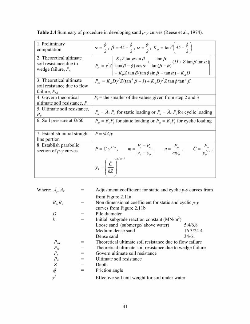
Table 2.4 Summary of procedure in developing sand p-y curves (Reese et al., 1974). 1. Preliminary computation 2

φα = , 2

45 φβ += , 2φα = , ⎟

⎠⎞

⎜⎝⎛ −=

245K 2

aφtan

2. Theoretical ultimate soil resistance due to wedge failure, Pst

⎥⎥⎥

⎦

⎤

⎢⎢⎢

⎣

⎡

−−+

+−

+−=

DKZK

ZDZKZP

a0

0

st

)tansin(tantan

)tantan()tan(

tancos)tan(sintan

'

αβφβ

αβφβ

βαφββφ

γ

3. Theoretical ultimate soil resistance due to flow failure, Psd

βφγβγ 40

8asd ZDK1ZDKP tantan)(tan '' +−=

4. Govern theoretical ultimate soil resistance, Ps

Ps = the smaller of the values given from step 2 and 3

5. Ultimate soil resistance, Pu ss

_

u PAP = for static loading or sc

_

u PAP = for cyclic loading

6. Soil pressure at D/60 ssm PBP = for static loading or scm PBP = for cyclic loading

7. Establish initial straight line portion

(kZ)y P =

8. Establish parabolic section of p-y curves

n/1_

yCP = , mu

mu

yyPP

m−−

= , m

m

myPn = , n/1

m

m_

yP

C = ,

1n/n_

k kZCy

−

⎟⎟⎟

⎠

⎞

⎜⎜⎜

⎝

⎛=

Where: c

__

s A,A = Adjustment coefficient for static and cyclic p-y curves from from Figure 2.11a Bs, Bc = Non dimensional coefficient for static and cyclic p-y curves from Figure 2.11b D = Pile diameter k = Initial subgrade reaction constant (MN/m3) Loose sand (submerge/ above water) 5.4/6.8 Medium dense sand 16.3/24.4 Dense sand 34/61 Psd = Theoretical ultimate soil resistance due to flow failure Pst = Theoretical ultimate soil resistance due to wedge failure Ps = Govern ultimate soil resistance Pu = Ultimate soil resistance Z = Depth φ = Friction angle = Effective soil unit weight for soil under water 'γ

41

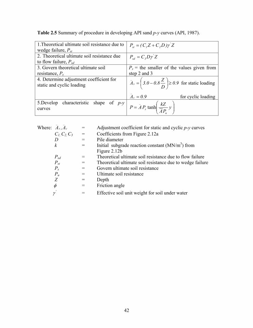
Table 2.5 Summary of procedure in developing API sand p-y curves (API, 1987). 1.Theoretical ultimate soil resistance due to wedge failure, Pst

Z)DCZC(P '21st γ+=

2. Theoretical ultimate soil resistance due to flow failure, Psd

ZDCP '3sd γ=

3. Govern theoretical ultimate soil resistance, Ps

Ps = the smaller of the values given from step 2 and 3

4. Determine adjustment coefficient for static and cyclic loading 9.0

DZ8.00.3As

_

≥⎟⎠⎞

⎜⎝⎛ −= for static loading

9.0Ac

_= for cyclic loading

5.Develop characteristic shape of p-y curves ⎟⎟

⎠

⎞⎜⎜⎝

⎛= y

PAkZPAP

us tanh

_

Where: c

_

s

_A,A = Adjustment coefficient for static and cyclic p-y curves

C1, C2, C3 = Coefficients from Figure 2.12a D = Pile diameter k = Initial subgrade reaction constant (MN/m3) from Figure 2.12b Psd = Theoretical ultimate soil resistance due to flow failure Pst = Theoretical ultimate soil resistance due to wedge failure

Ps = Govern ultimate soil resistance Pu = Ultimate soil resistance Z = Depth φ = Friction angle = Effective soil unit weight for soil under water 'γ

42

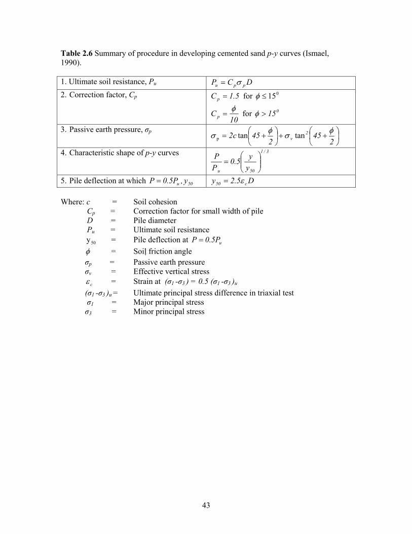
Table 2.6 Summary of procedure in developing cemented sand p-y curves (Ismael, 1990). 1. Ultimate soil resistance, Pu DCP ppu σ= 2. Correction factor, Cp 5.1C p = for 015≤φ

10C p

φ= for 015>φ

3. Passive earth pressure, σp⎟⎠⎞

⎜⎝⎛ ++⎟

⎠⎞

⎜⎝⎛ +=

245

245c2 2

vφσφσ tantanp

4. Characteristic shape of p-y curves 3/1

50u yy5.0

PP

⎟⎟⎠

⎞⎜⎜⎝

⎛=

5. Pile deflection at which 50u y,0.5PP = D5.2y c50 ε= Where: c = Soil cohesion Cp = Correction factor for small width of pile D = Pile diameter Pu = Ultimate soil resistance 50y = Pile deflection at u0.5PP = φ = Soil friction angle σp = Passive earth pressure σv = Effective vertical stress cε = Strain at (σ1 -σ3 ) = 0.5 (σ1 -σ3 )u

(σ1 -σ3 )u = Ultimate principal stress difference in triaxial test σ1 = Major principal stress σ3 = Minor principal stress

43

CHAPTER 3

NUMERICAL MODELING

3.1 INTRODUCTION

The finite element code ABAQUS is used in this study to model the soil-pile-

structure interaction problem. This chapter presents and discusses the details of the

numerical modeling. The non-linear constitutive soil model used for this study is

discussed first followed by a discussion of a modified interface subroutine used to model

the soil-pile interface. Boundary condition used to simulate the infinite medium that

surrounds the soil-pile models is discussed next. Finally, a validation of the FE model is

presented.

3.2 CONSTITUTIVE SOIL MODEL

Soil generally shows nonlinear behavior when subject to shear loading. The

secant shear modulus decreases with increasing shear strain while material damping

increases (Hardin and Drnevich 1972). These changes in material properties affect the

SPSI behavior. In order to simulate the observed behavior of soils, a non-linear

constitutive model is required. Generally, soil models based on work hardening theory

are used for this purpose. The multiaxial cyclic plastic model for clay developed by Borja

and Amies (1994) and implemented in a FE code by Rodriguez-Marek (2000) was used

in this study. The original model by Borja and Amies (1994) was later modified by Borja

et al. (1999). For the purpose of this thesis, this updated model will be referred to as

Borja’s model. Borja’s model works well for cohesive soils under undrained loading (e.g.

Borja and Amies 1994, Borja et al. 1999, Rodriguez-Marek 2000).

44

Borja’s model, based on total stress, was constructed through the reformulation of

the Dafalias and Popov (1977) bounding surface plasticity constitutive model to

accommodate multi-axial stress reversals. The model was developed based on a

vanishing elastic region undergoing pure translation inside a bounding surface, and an

exponential function for the hardening modulus H΄, which changes with the tensorial

distance between the current stress state and the recent unloading point (Borja and Amies

1994). The concept of the vanishing elastic region allows for the modeling of plastic

strains developed at small strains. Borja’s model includes criteria for loading and

unloading that are applicable to general stress states; i.e. the hardening modulus should

decrease monotonically with deformation under continued loading. Since the model is

based on total stress, the excess pore pressures induced by seismic loading cannot be

predicted. This feature is not a significant limitation if the model is used for non-

liquefiable soils subject to rapid loading (e.g. seismic loading, see Rodriguez-Marek

2000, Rodriguez-Marek and Bray 2005).

3.2.1 General description

Figure 3.1 shows a schematic representation of the constitutive model. The

surfaces defined by F and B are two J2 type functions that represent the yield function and

bounding surface, respectively. The vanishing elastic region corresponds to the limit

when the size of F is zero at an unloading point. The coordinates in the'oσ π plane

(Figure 3.1) represent the location of the vanishing elastic region.

The point Fo, with coordinates , represents a point where the soil experienced

the most recent elastic unloading. F

'oσ

o can be located inside or on the bounding surface.

The value of the hardening parameter H΄ changes from infinity at Fo to a constant Ho at

45

surface B. In other words, the soil is assumed to behave elastically at point Fo and to

follow a linear kinematic hardening plasticity law at the bounding surface B. For any

point that exists between Fo and surface B, H΄ is interpolated using the exponential

function described in section 3.2.3. The yield function F passes through the current stress

coordinates . The shape of the contours of equal H΄ are centered around F'σ o and

depend on the interpolation function. These contours do not need to be circular. The

coordinate point at the surface B represents the image point created in such a way that

coordinate points , , and have to be in a straight line in the

∧'σ

'oσ 'σ

∧'σ π plane. The

exponential interpolation function of the hardening modulus H΄ is generated from well-

accepted one-dimensional models for soils (Borja and Amies 1994).

46

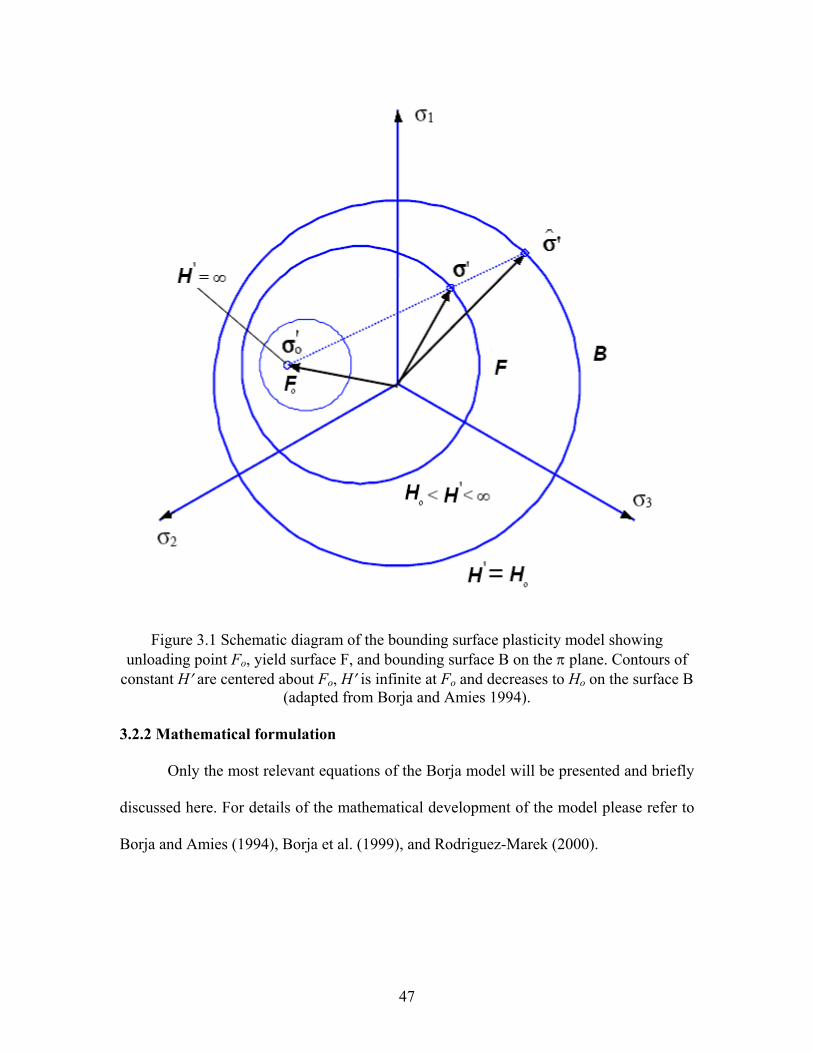
Figure 3.1 Schematic diagram of the bounding surface plasticity model showing unloading point Fo, yield surface F, and bounding surface B on the π plane. Contours of

constant H′ are centered about Fo, H′ is infinite at Fo and decreases to Ho on the surface B (adapted from Borja and Amies 1994).

3.2.2 Mathematical formulation

Only the most relevant equations of the Borja model will be presented and briefly

discussed here. For details of the mathematical development of the model please refer to

Borja and Amies (1994), Borja et al. (1999), and Rodriguez-Marek (2000).

47

Additive decomposition of the strain tensor is assumed. Therefore the total

tensorial strain rate (ε& ) can be divided in to two parts; elastic strain rate ( ) and plastic

strain rate ( ),

eε&

pε&

(3.1) pe εεε &&& +=

where the dot represents the first differential with respect to time and an associated flow

rule is used to find the . The generalized Hooke’s law is used to find the total tensorial

stress rate with respect to elastic strain rate.

pε&

(3.2) )(: peC εεσ &&& −=

where σ& is the total tensorial stress rate, is the rank four elasticity tensor, and the

colon denotes an inner product. The soil is assumed to behave as a decoupled material.

Hence, elastic volumetric and shear strain can be treated separately.

eC

Plastic strains are associated with the yield surface F and the bounding surface B.

The yield function F has the form of a J2 type plasticity model:

(3.3) 0: 2 =−′′= rF ξξ

where ξ' = σ' – α is a translated deviatoric stress tensor, r is the radius of the yield

function, σ ′ is the deviatoric part of σ , and α is the deviatoric back stress tensor

representing the center of F. Note that plastic volumetric strains are assumed to be zero.

The Prager translation rule is used to calculate the back stress (Prager 1956).

Similarly, the bounding surface B has the form of a J2 type plasticity model:

(3.4) 0: 2 =−′′= RB σσ

where R > r is the radius of the bounding surface B centered about the hydrostatic axis.

In soils, R can be correlated to the undrained shear strength, su, by

48

usR ×=38 (3.5)

where su can be obtained from an unconfined compressive strength test. Using equations

3.1 to 3.4, a rate constitutive equation can be obtained as (see Borja and Amies 1994):

K=σ& )(ε&tr 1 + 2 G ε ′⎟⎠⎞

⎜⎝⎛

′+

−

&131

HG (3.6)

where K is the elastic bulk modulus, G is the small strain shear modulus, 1 is the rank two

identity tensor, and tr is the trace operator.

3.2.3 Hardening function

The hardening modulus H΄ is defined in such a way as to fit well-accepted one-

dimensional cyclic stress-strain relationships. Following the Dafalias and Popov (1977)

idea, the hardening modulus H΄ is obtained from an interpolation between the elastic

value (H΄=infinity) at the last unloading point Fo and a limiting value of Ho at the

bounding surface B. A criterion for loading and unloading is described in the following

section.

An exponential hardening modulus, validated by Borja et al. (1999 and 2000) by

comparison with experimental modulus reduction and damping curves, is considered for

this study. The exponential hardening modulus can be expressed as:

(3.7) om HhH +=′ κ

where h and m are the parameters of the model. The parameter h controls the rate of

shear stiffness degradation and the parameter m is a dimensionless parameter that

controls the shape of the secant modulus values versus the strain amplitude curve. The

variable κ is a dimensionless scalar quantity that should satisfy the following condition:

49

( ) Ro =′−′+′ σσκσ (3.8)

The hardening modulus H΄ varies with κ in such a way that the limiting conditions

discussed above are satisfied. That is, when σ ′ is at the last unloading point then κ is

infinity hence H' is also infinity. On the other hand, when σ ′ is at the bounding surface

then κ should be zero in order to satisfy Equations 3.7 and 3.8.

3.2.4 Loading and unloading conditions

When solving numerical problems with known monotonic loadings, it is

important to define whether the current strain increment is in a loading or unloading

condition. When the stresses are on the bounding surface, the loading and unloading

conditions are defined by the Kuhn-Tucker conditions (Simo and Hughes 1998). For any

given yield function f, these conditions are given by:

0>λ , 0f ≤ , and 0f =λ (3.9)

where λ is the consistency parameter and f is the given yield surface. A return mapping

algorithm (Simo and Hughes 1998) is used for strain increments on the bounding surface.

Different loading/unloading conditions have to be used within the bounding

surface because the singularity that results from the zero radius of the elastic region

renders the Kuhn-Tucker loading conditions ill defined. Borja and Amies (1994) define

unloading as the condition when the direction of the load step results in an increase of the

hardening modulus. Consequently, the loading condition is postulated as

( ) ( )( )

( )0:

:11

2oo

o >′′−′+′−′′

′−′++′+− ε

σσκσσσ

σσκκσκ& (3.10)

Upon unloading, the position of Fo will be shifted to the current position of the

stress tensor σ′. For the numerical implementation of Equation 3.10, see Borja and Amies

50

(1994). Additional conditions are imposed on the loading-unloading criteria to prevent

unloading under infinitesimal strains that may result from numerical noise (Rodriguez-

Marek 2000). The model is only permitted to unload when the magnitude of the strain

reversal exceeds the elastic threshold of the soil.

3.2.5 Rayleigh’s damping

Laboratory tests have shown that damping at high strain is independent of

frequency and hysteretic behavior alone can explain energy dissipation in laboratory

tests. On the other hand, experimental results in the small strain range indicated that

hysteretic behavior alone cannot account for the measured damping levels (Lanzo and

Vucetic 1999). Typically, damping at low strains is small and can be modeled as

equivalent viscous damping. The viscous damping coefficient for a given frequency ωi

can be expressed in terms of critical damping, iξ , as:

22

iR

i

Ri

ωβω

αξ += (3.11)

where Rα is mass proportional damping and Rβ is stiffness proportional damping.

However, in this study critical damping is considered to be a constant across frequencies.

To approximate this Equation 3.11 can be reorganized in the following way:

22

iR

i

R ωβω

αξ += (3.12)

21

21R

2ωω

ξωωα+

= (3.12a)

21

R2

ωωξβ

+= (3.12b)

51

By an adequate selection of 1ω and 2ω , ξ is rendered constant over the range of

frequency of interest. Figure 3.2 illustrates the dependence of mass and stiffness

proportional damping on frequency. The effect of mass proportional damping is very low

at high frequencies. On the other hand, stiffness proportional damping is very low at low

frequencies. Therefore, the combination of both damping types allows a fit for the desired

value of damping ratio within a selected range of frequencies (i.e., close to and between

1ω and 2ω ). Between 1ω and 2ω , the resulting damping is however lower than the

desired critical damping and away from this range, the system is over damped. 1ω and

2ω are selected in such a way that the natural frequency of the soil deposit and the

frequencies of the interest (e.g. loading frequency) are within the range of 1ω and 2ω

(Hudson et al. 1994).

Some constitutive models are readily available in the ABAQUS FE program. The

user can also incorporate a user-defined constitutive model through a subroutine named

umat. This subroutine operates on each integration point by receiving variables such as

the incremental strain vector and the previous stress vector, and returning the current

stress vector and the Jacobian matrix (current tangent modulus matrix). Furthermore, the

user can update the solution dependent state variable and model variables (e.g.

parameters h, m for Borja’s model) for the next iteration step.

Mass proportional damping can be incorporated directly in the ABAQUS FE code

for built-in constitutive models (ABAQUS 2005). However, for a user material, stiffness

proportional damping must be incorporated in the user material subroutine (umat). This is

achieved by adding the stress due to stiffness proportional damping, dσ , to the stress

resulting from the constitutive response at each integration point:

52

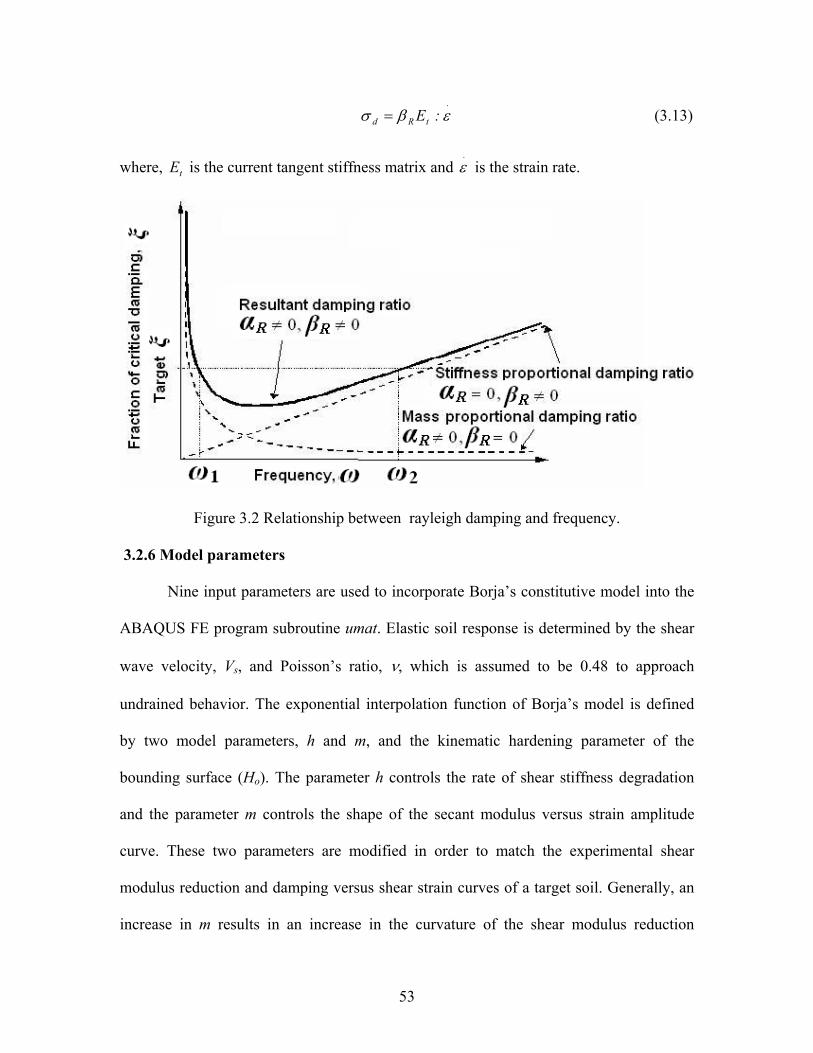
(3.13) .

tRd :E εβσ =

where, is the current tangent stiffness matrix and is the strain rate. tE.ε

Figure 3.2 Relationship between rayleigh damping and frequency.

3.2.6 Model parameters

Nine input parameters are used to incorporate Borja’s constitutive model into the

ABAQUS FE program subroutine umat. Elastic soil response is determined by the shear

wave velocity, Vs, and Poisson’s ratio, ν, which is assumed to be 0.48 to approach

undrained behavior. The exponential interpolation function of Borja’s model is defined

by two model parameters, h and m, and the kinematic hardening parameter of the

bounding surface (Ho). The parameter h controls the rate of shear stiffness degradation

and the parameter m controls the shape of the secant modulus versus strain amplitude

curve. These two parameters are modified in order to match the experimental shear

modulus reduction and damping versus shear strain curves of a target soil. Generally, an

increase in m results in an increase in the curvature of the shear modulus reduction

53

curves, while an increase in h causes a shift to the right of shear modulus reduction and

damping curves (Rodriguez-Marek 2000). Soil strength is defined by the radius of the

bounding surface, R (Equation 3.5). If the soil will not reach shear failure, the parameter

R can be used as a curve fitting parameter. Rayleigh stiffness proportional damping is

defined by the coefficient Rβ . Note that mass proportional damping is entered as an input

parameter in the program execution, and does not need to be entered in the user-defined

subroutine. Soil density and trapezoidal integration parameter, β, must also be defined

(for more detail refer to Rodriguez-Marek 2000).

3.3 INTERFACE MODEL

In ABAQUS, mechanical contact between two bodies (surfaces) can be modeled

by using surfaces that may interact (it is noted that ABAQUS can also operate in an

explicit mode. Contact interaction in the explicit mode allows for different option. In this

work, ABAQUS is used only in the implicit option). On the other hand, mechanical

contact between two nodes can be modeled by using contact elements. Contact elements

can be used when contact between two bodies cannot be simulated with the surface based

contact approach. In this study the former approach is considered. Generally, interface

modeling has three steps:

1. define the contact surfaces which could potentially be in contact,

2. state which surfaces interact with one another,

3. define the mechanical (tangent and normal) and thermal properties of the surface.

In the surfaced based contact approach, two surfaces have to be defined based on their

rigidity: the more deformable surface is defined as a slave surface and the more rigid

surface is defined as a master surface. Master surfaces should be defined as an element

54

based surface. However, slave surfaces can be defined as either element based or node

based surfaces. In this study both options are used depending on the analysis problem.

The tangent and normal behavior are defined through Coulomb friction and a modified

hard contact, respectively. In the modified hard contact approach, tensile stress can be

transferred between two surfaces up to the maximum tensile stress specified by the user

(ABAQUS 2005). In this approach, when surfaces are in contact, surfaces transmit shear

and normal stress across their interface.

In this analysis geostatic stress is not applied to the finite element mesh because

of problems related to static boundary conditions for the dynamic model. However, the

contact interaction between soil and pile is a function of overburden stress because soil-

pile separation does not occur until the existing overburden stress is overcome. This can

be achieved by a modified hard contact approach. That is, a modified hard contact is used

to allow tension stresses up to the overburden horizontal confining pressure, which is

entered as an input parameter. Moreover, frictional resistance is a function of overburden

stress. Therefore, the standard Coulomb friction model in ABAQUS was modified by

using subroutine fric to include a cohesion (C΄) component and to account for the

additional resistance ( ) due to overburden stresses. The modified critical shear stress op

)( critτ is defined through the relation:

(3.14) )pp(C alo'

crit ++= µτ

where, µ is the friction coefficient, is contact pressure due to geostatic (overburden)

load, and is the contact pressure due to the applied load. ,

op

alp 'C µ , and are the input

parameters for the subroutine fric. The pile is divided into several surfaces along the

op

55

depth in order to incorporate the change in with depth. The modified coulomb friction

criteria is then defined as:

op

crit22

21eq ττττ ≤+= (3.15)

where, eqτ is equivalent frictional stress, 1τ and 2τ are shear stress in direction one and

two, respectively. The standard coulomb friction model assumes that if Equation 3.15 is

satisfied then there is no relative motion between surfaces. However, for convergence

reasons, elastic slip is allowed for this model; that is, a controlled amount of elastic shear

deformation ( critγ ) is allowed before slippage takes place. In this study, critγ is selected as

0.5% of the average length of all contact elements in the model. The elastic slip can be

related to interface shear stress in the following way:

(3.16a) elisi k γτ =

crit

critsk

γτ

= (3.16b)

where, is the (current) “ stiffness in stick.” Equation 3.16a is valid if Equation 3.15 is

satisfied. If Equation 3.15 is not satisfied, then the frictional shear stresses are given by:

sk

))pp(C( alo'

eq

icrit

eq

ii ++== µ

γγτ

γγτ (3.17a)

where,

22

21eq γγγ += (3.17b)

56

3.4 TRANSMITTING BOUNDARY CONDITION

Transmitting boundary conditions as described in section 2.3.1 are used to reduce

wave reflections at model boundaries. Since geostatic stress is not applied to the model,

static boundary conditions are not necessary for this model. However, in order to

simulate the infinite medium during the seismic analysis, the FE model needs some kind

of seismic boundary condition. In this section, the free field boundary used at the lateral

boundaries of the model is described first followed by the description of the quiet

boundaries used to simulate the semi-infinite half space at the base.

3.4.1 Free-field boundaries

The displacement at the lateral boundaries should be equal to that of a free field

soil column. The free field motion refers to the motion in the absence of structural or

foundation elements. If soil material damping is high, then free field response can be

achieved using a reasonably small distance from the model structure to the edge of the

model. However, when the material damping is low, free field response is difficult to

achieve with a limited distance from the model structure to the edge of the model. An

alternative approach is to “enforce” the free field motion in such a way that boundaries

act as an absorbing mechanism. This can be modeled by coupling viscous dashpots

between main model nodes to soil column nodes at the edges (refer to Figure 3.3), which

represent the free field motion. The side boundary nodes of the main model and the soil

column nodes should have matching coordinates. Note that this boundary condition only

applies if the sides of the main model are vertical. The following governing equations are

used to determine the absorbed energy by the viscous dashpots:

(3.18a) A)vv(CF ffn

mnpn −−= ρ

57

(3.18b) A)vv(CF fft

mtst −−= ρ

where, ρ is the density of the soil material, is the P-wave speed at the side boundary,

is the S- wave speed at the side boundary, is the area of influence of the free-field

node, is the normal velocity of the node which is at the side of the main soil model,

is the tangential velocity of the node which is at the lateral boundary of the main soil

model, is the normal velocity of the soil column node adjacent to the boundary node,

and is the tangential velocity of the soil column node adjacent to the boundary node.

pC

sC A

mnv

mtv

ffnv

fftv

In this study, dashpot coefficients, ACC pn ρ= and ACC st ρ= , are input

parameters. The soil columns on the edge of the model have a single degree of freedom

in the direction of load application (thus modeling 1-D wave propagation in the free field)

and the side nodes of the main soil model are restricted to have only horizontal motion.

The soil columns in the boundaries can be made to respond to the input motion, or for

computational efficiency, free field displacements with time, computed separately, can be

given as boundary conditions for the soil column nodes.

58

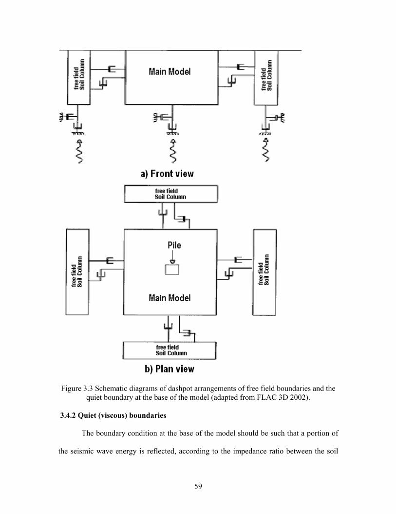
Figure 3.3 Schematic diagrams of dashpot arrangements of free field boundaries and the quiet boundary at the base of the model (adapted from FLAC 3D 2002).

3.4.2 Quiet (viscous) boundaries

The boundary condition at the base of the model should be such that a portion of

the seismic wave energy is reflected, according to the impedance ratio between the soil

59

model and the underlying half space representing bedrock. A quiet boundary scheme

proposed by Lysmer and Kuhlemeyer (1969) is used to simulate this type of boundary

condition. Viscous dashpots are attached in the normal and tangential directions at the

base of the model in order to reflect some portion of the energy to the main soil model.

The governing equations are similar to 3.18a and 3.18b but free field velocity is zero and

density refers to the bedrock density. Viscous dashpots are attached in all three

perpendicular directions in this study.

3.5 LOADING

In a seismic analysis, seismic load can be applied either as a displacement,

acceleration, or velocity time history at the base of the model; or as a body force per unit

volume for the entire mesh as is described in section 2.1.3. Relative motions

(displacement, acceleration, velocity) will be output when load is applied as body force

per unit volume for the entire mesh (e.g., the output is the motion of the mesh relative to

the motion at the base). In this study, seismic load is applied as a shear stress at the base

because a quiet boundary condition and displacement boundary condition cannot be

applied simultaneously. The shear force in the viscous dashpots at the base of the model

is proportional to velocity. Hence, the application of shear force at the base is equivalent

to applying a velocity time history at the base of the model. A similar scheme is used in

the finite difference code FLAC 3D (FLAC 3D 2002). Validation of this loading scheme

is presented in section 3.6.1.

3.6 MODEL VALIDATION

The model used in this study is validated for its applicability to the soil-pile

interaction problem. The load application method is validated first. Pile element size and

60

the model dimensions need to be adequate for the study; hence a parametric study of the

effect of model and mesh size is also performed. The use of stiffness proportional

damping, also an important aspect in this study, is validated next. Finally, a brief

discussion of the overall validation of the model is presented.

3.6.1 Validation of the load application method

Initially, a 3-D FE mesh was built to represent a soil column with a height of 10 m

and 1 m width in both horizontal directions (see Figure 3.4). The soil column consists of

ten 8-node tri-linear brick elements with unit area. In this validation, soil column motion

was restrained in two directions (vertical and one horizontal); that is, every node has only

one degree of freedom in one horizontal direction, hence modeling one-dimensional shear

wave propagation. A sine sweep equation given by equation 3.19 was used to generate

the acceleration input motion:

(3.19) ))tt(*)tt((Sin))tt(A()tt(a 2 ∆∆ω∆∆ +++=+

)t/t/()t()tt( t ∆ω∆ω∆ω +=+

)t/t/(A)t(A)tt(A u ∆∆∆ +=+ for utt ≤

EA)tt(A =+ ∆ for cuu tttt +≤<

)t/t/(A)t(A)tt(A d ∆∆∆ −=+ for cu ttt +>

where is low frequency, is high frequency, lf hf ω∆ is given by 2π(fh-fl), is start

amplitude , is end amplitude, ∆A is given by A

SA

EA e – As, , is ramp up time, is

constant amplitude time, is ramp down time (total time, t

ut ct

dt t, is given by dcut tttt ++= )

and t∆ is the time step. The initial conditions for the above equation are A(0) = As and

ω(0) = 2πfl.

61

The acceleration time history was integrated to get velocity. A base line

correction was performed on the motion to ensure zero final velocity. A linear elastic

model was used for the soil. The Young’s modulus and Poisson’s ratio were set to

5.328x108 N/m2 and 0.48 (corresponding to Vs of 300 m/s), respectively and the density

was taken as 2000 kg/m3.

Shear stress was obtained from:

)()( tVVt SS ρσ = (3.20)

where, ρ is density of the rock (basement), is rock shear velocity, and is the rock

outcrop velocity time history. The shear stress was applied at the base of the soil column

simultaneously with quiet boundary conditions corresponding to rock properties (ρ=2300

kg/m

SV )(tV

3, Vs=1000 m/s) in order to simulate the base rock. Response was obtained at the top

node of the soil column. From this analysis, the transfer function (TF) between the top of

the soil and the input (rock) motion was obtained by using the Fast Fourier Transfer

(FFT). This TF was compared with the TF obtained from the analytical equation given by

Kramer (1996). Figure 3.5 shows that the TF obtained in both cases are similar up to 15

Hz. Therefore, seismic load can be applied as a shear stress time history at the base for all

analyses.

62

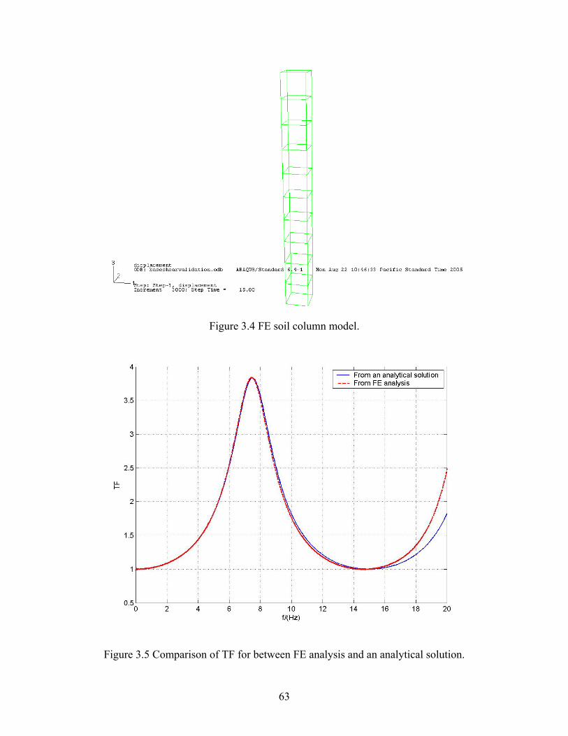
Figure 3.4 FE soil column model.

Figure 3.5 Comparison of TF for between FE analysis and an analytical solution.

63

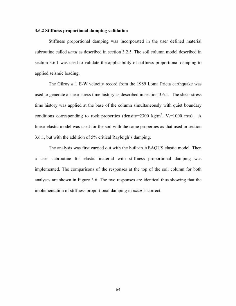
3.6.2 Stiffness proportional damping validation

Stiffness proportional damping was incorporated in the user defined material

subroutine called umat as described in section 3.2.5. The soil column model described in

section 3.6.1 was used to validate the applicability of stiffness proportional damping to

applied seismic loading.

The Gilroy # 1 E-W velocity record from the 1989 Loma Prieta earthquake was

used to generate a shear stress time history as described in section 3.6.1. The shear stress

time history was applied at the base of the column simultaneously with quiet boundary

conditions corresponding to rock properties (density=2300 kg/m3, Vs=1000 m/s). A

linear elastic model was used for the soil with the same properties as that used in section

3.6.1, but with the addition of 5% critical Rayleigh’s damping.

The analysis was first carried out with the built-in ABAQUS elastic model. Then

a user subroutine for elastic material with stiffness proportional damping was

implemented. The comparisons of the responses at the top of the soil column for both

analyses are shown in Figure 3.6. The two responses are identical thus showing that the

implementation of stiffness proportional damping in umat is correct.

64

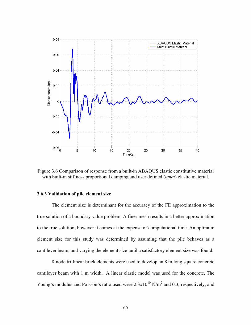
Figure 3.6 Comparison of response from a built-in ABAQUS elastic constitutive material with built-in stiffness proportional damping and user defined (umat) elastic material.

3.6.3 Validation of pile element size

The element size is determinant for the accuracy of the FE approximation to the

true solution of a boundary value problem. A finer mesh results in a better approximation

to the true solution, however it comes at the expense of computational time. An optimum

element size for this study was determined by assuming that the pile behaves as a

cantilever beam, and varying the element size until a satisfactory element size was found.

8-node tri-linear brick elements were used to develop an 8 m long square concrete

cantilever beam with 1 m width. A linear elastic model was used for the concrete. The

Young’s modulus and Poisson’s ratio used were 2.3x1010 N/m2 and 0.3, respectively, and

65

the density used was 2400 kg/m3. One edge of the beam was fixed while the other edge

was loaded with a point load of 2000 N. Displacements along the cantilever were

obtained for different element sizes. Then these displacements were compared with the

displacements obtained from beam theory:

)L6

x2x(

EIPL)x(y

32

−−= (3.21)

where, P is the applied point load, L is length of the cantilever beam, E is Young’s

modulus of the cantilever beam, x is distance from the fixed edge, and I is second

moment of the inertia.

Figure 3.7 shows the comparison of the displacement for FE models with

different sized elements and the displacements from elastic beam theory. A minimum of

sixteen elements along the pile are needed to approximate the analytical solution.

Similarly, eight elements in the cross section of the pile are required to get a good

approximation to the solution.

66

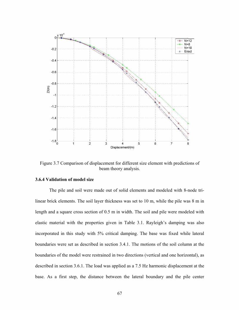
Figure 3.7 Comparison of displacement for different size element with predictions of beam theory analysis.

3.6.4 Validation of model size

The pile and soil were made out of solid elements and modeled with 8-node tri-

linear brick elements. The soil layer thickness was set to 10 m, while the pile was 8 m in

length and a square cross section of 0.5 m in width. The soil and pile were modeled with

elastic material with the properties given in Table 3.1. Rayleigh’s damping was also

incorporated in this study with 5% critical damping. The base was fixed while lateral

boundaries were set as described in section 3.4.1. The motions of the soil column at the

boundaries of the model were restrained in two directions (vertical and one horizontal), as

described in section 3.6.1. The load was applied as a 7.5 Hz harmonic displacement at the

base. As a first step, the distance between the lateral boundary and the pile center

67

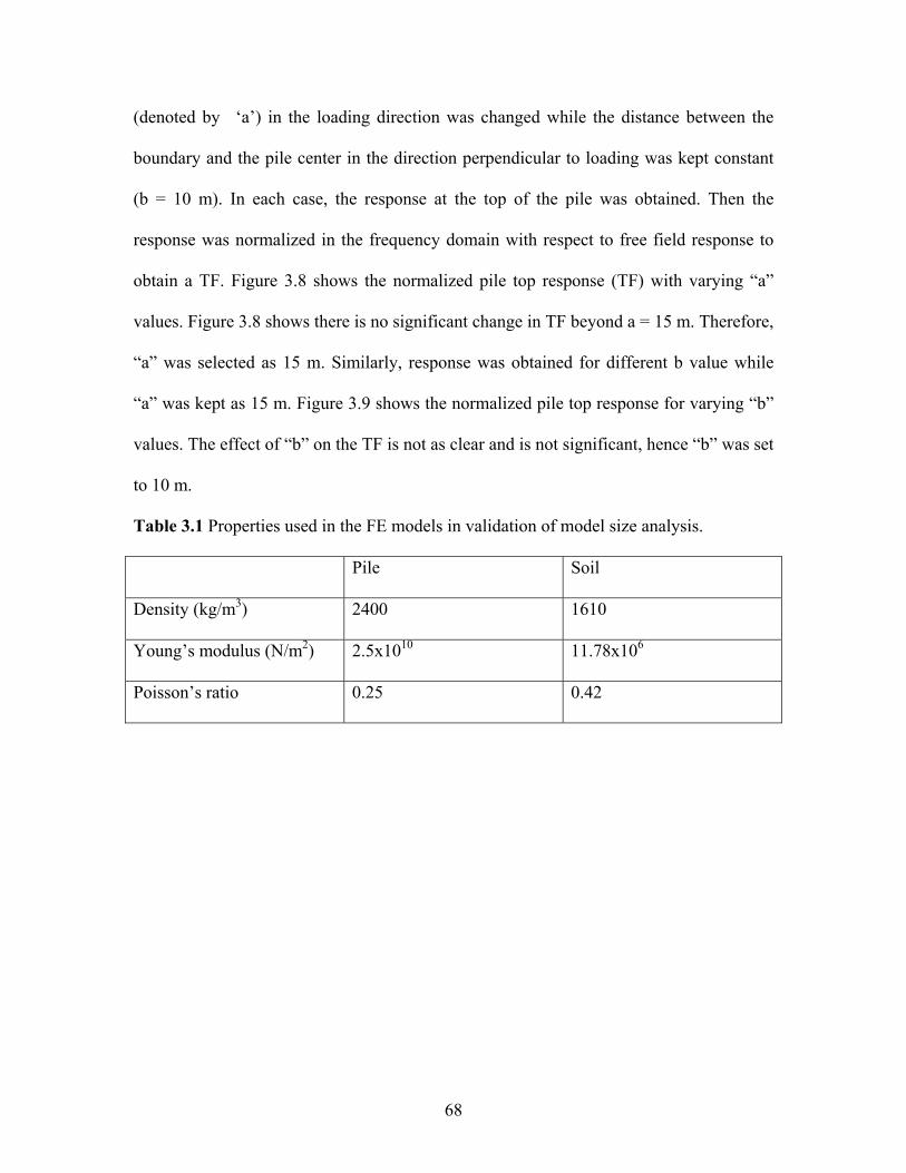
(denoted by ‘a’) in the loading direction was changed while the distance between the

boundary and the pile center in the direction perpendicular to loading was kept constant

(b = 10 m). In each case, the response at the top of the pile was obtained. Then the

response was normalized in the frequency domain with respect to free field response to

obtain a TF. Figure 3.8 shows the normalized pile top response (TF) with varying “a”

values. Figure 3.8 shows there is no significant change in TF beyond a = 15 m. Therefore,

“a” was selected as 15 m. Similarly, response was obtained for different b value while

“a” was kept as 15 m. Figure 3.9 shows the normalized pile top response for varying “b”

values. The effect of “b” on the TF is not as clear and is not significant, hence “b” was set

to 10 m.

Table 3.1 Properties used in the FE models in validation of model size analysis.

Pile Soil

Density (kg/m3) 2400 1610

Young’s modulus (N/m2) 2.5x1010 11.78x106

Poisson’s ratio 0.25 0.42

68

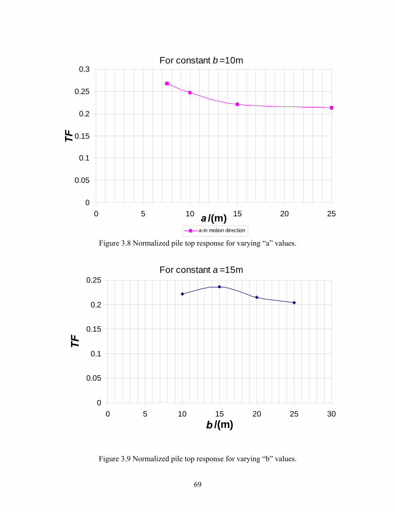
For constant b =10m

0

0.05

0.1

0.15

0.2

0.25

0.3

0 5 10 15 20 25a /(m)

TF

a-in motion direction

Figure 3.8 Normalized pile top response for varying “a” values.

For constant a =15m

0

0.05

0.1

0.15

0.2

0.25

0 5 10 15 20 25 30b /(m)

TF

Figure 3.9 Normalized pile top response for varying “b” values.

69

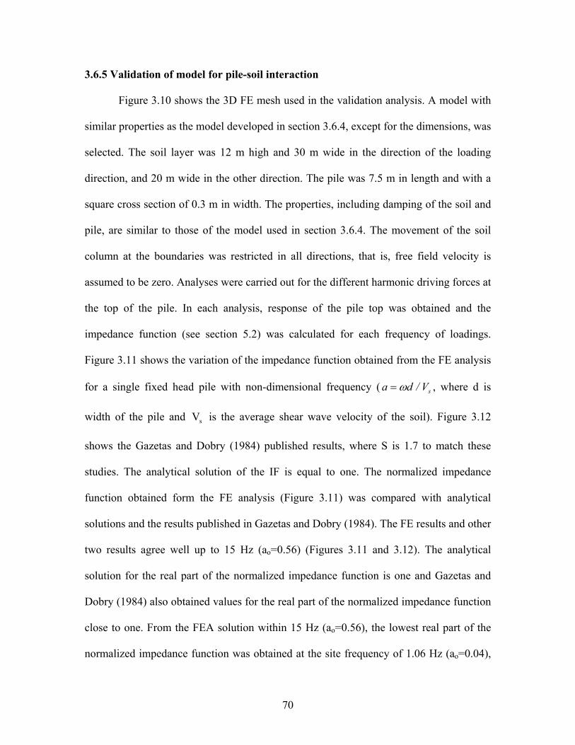
3.6.5 Validation of model for pile-soil interaction

Figure 3.10 shows the 3D FE mesh used in the validation analysis. A model with

similar properties as the model developed in section 3.6.4, except for the dimensions, was

selected. The soil layer was 12 m high and 30 m wide in the direction of the loading

direction, and 20 m wide in the other direction. The pile was 7.5 m in length and with a

square cross section of 0.3 m in width. The properties, including damping of the soil and

pile, are similar to those of the model used in section 3.6.4. The movement of the soil

column at the boundaries was restricted in all directions, that is, free field velocity is

assumed to be zero. Analyses were carried out for the different harmonic driving forces at

the top of the pile. In each analysis, response of the pile top was obtained and the

impedance function (see section 5.2) was calculated for each frequency of loadings.

Figure 3.11 shows the variation of the impedance function obtained from the FE analysis

for a single fixed head pile with non-dimensional frequency ( sV/da ω= , where d is

width of the pile and is the average shear wave velocity of the soil). Figure 3.12

shows the Gazetas and Dobry (1984) published results, where S is 1.7 to match these

studies. The analytical solution of the IF is equal to one. The normalized impedance

function obtained form the FE analysis (Figure 3.11) was compared with analytical

solutions and the results published in Gazetas and Dobry (1984). The FE results and other

two results agree well up to 15 Hz (a

sV

o=0.56) (Figures 3.11 and 3.12). The analytical

solution for the real part of the normalized impedance function is one and Gazetas and

Dobry (1984) also obtained values for the real part of the normalized impedance function

close to one. From the FEA solution within 15 Hz (ao=0.56), the lowest real part of the

normalized impedance function was obtained at the site frequency of 1.06 Hz (ao=0.04),

70

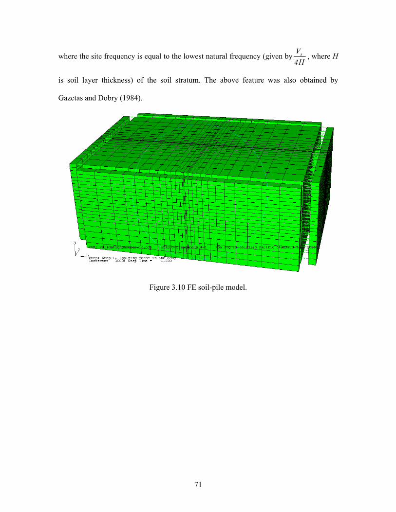
where the site frequency is equal to the lowest natural frequency (given byH4

Vs , where H

is soil layer thickness) of the soil stratum. The above feature was also obtained by

Gazetas and Dobry (1984).

Figure 3.10 FE soil-pile model.

71

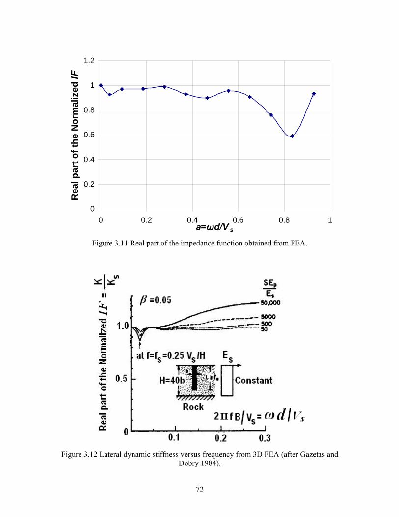
0

0.2

0.4

0.6

0.8

1

1.2

0 0.2 0.4 0.6 0.8 1a=ωd/V s

Rea

l par

t of t

he N

orm

aliz

ed IF

Figure 3.11 Real part of the impedance function obtained from FEA.

Figure 3.12 Lateral dynamic stiffness versus frequency from 3D FEA (after Gazetas and

Dobry 1984).

72

CHAPTER 4

PARAMETRIC STUDY ON KINEMATIC INTERACTION

4.1 INTRODUCTION

A parametric study was conducted in order to understand the effect of several

variables on the kinematic interaction of a fixed-head single pile. In this study, the effects

of pile diameter, soil non-linearity, gapping, and intensity of the input ground motion

were considered. The effect of these variables on the transfer function (see Section 2.2.1)

is studied. In addition the effects of these variables on the kinematic stress in a fixed-head

single pile are also considered. The results of the parametric study will provide a better

understanding of the effect of kinematic interaction on the dynamic behavior of a fixed-

head single pile.

4.2 COMPUTATION OF THE TRANSFER FUNCTION

The transfer function (TF) of the pile is required in order to find the input motion for

the analysis of the super structure supported by pile foundations. Figure 4.1 illustrates a

fixed-head pile-soil system excited by vertically propagating harmonic shear waves

( )tiexp(U g ω ). These harmonic shear waves would produce a harmonic oscillation,

termed “free field” oscillation, of )tiexp(U ff ω at a point in the ground surface which is

far enough from the pile to have no effects due to the presence of the pile. The frequency

dependent transfer function (TF) can be calculated from the following equation:

( )( )( )fU

fUfTF

ff

p= 4.1

where, ( )fU p is the maximum lateral response at the pile top for a given excitation

frequency f. This definition of the transfer function was used also by Kim and Stewart

73

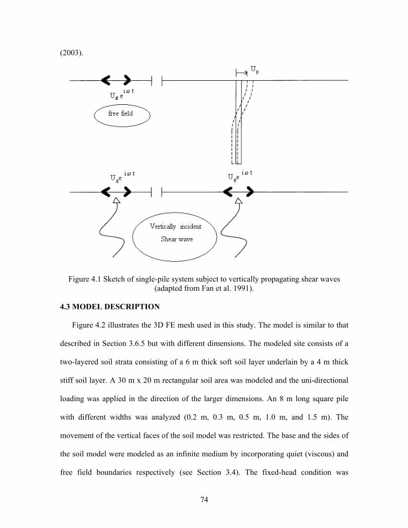
(2003).

Figure 4.1 Sketch of single-pile system subject to vertically propagating shear waves (adapted from Fan et al. 1991).

4.3 MODEL DESCRIPTION

Figure 4.2 illustrates the 3D FE mesh used in this study. The model is similar to that

described in Section 3.6.5 but with different dimensions. The modeled site consists of a

two-layered soil strata consisting of a 6 m thick soft soil layer underlain by a 4 m thick

stiff soil layer. A 30 m x 20 m rectangular soil area was modeled and the uni-directional

loading was applied in the direction of the larger dimensions. An 8 m long square pile

with different widths was analyzed (0.2 m, 0.3 m, 0.5 m, 1.0 m, and 1.5 m). The

movement of the vertical faces of the soil model was restricted. The base and the sides of

the soil model were modeled as an infinite medium by incorporating quiet (viscous) and

free field boundaries respectively (see Section 3.4). The fixed-head condition was

74

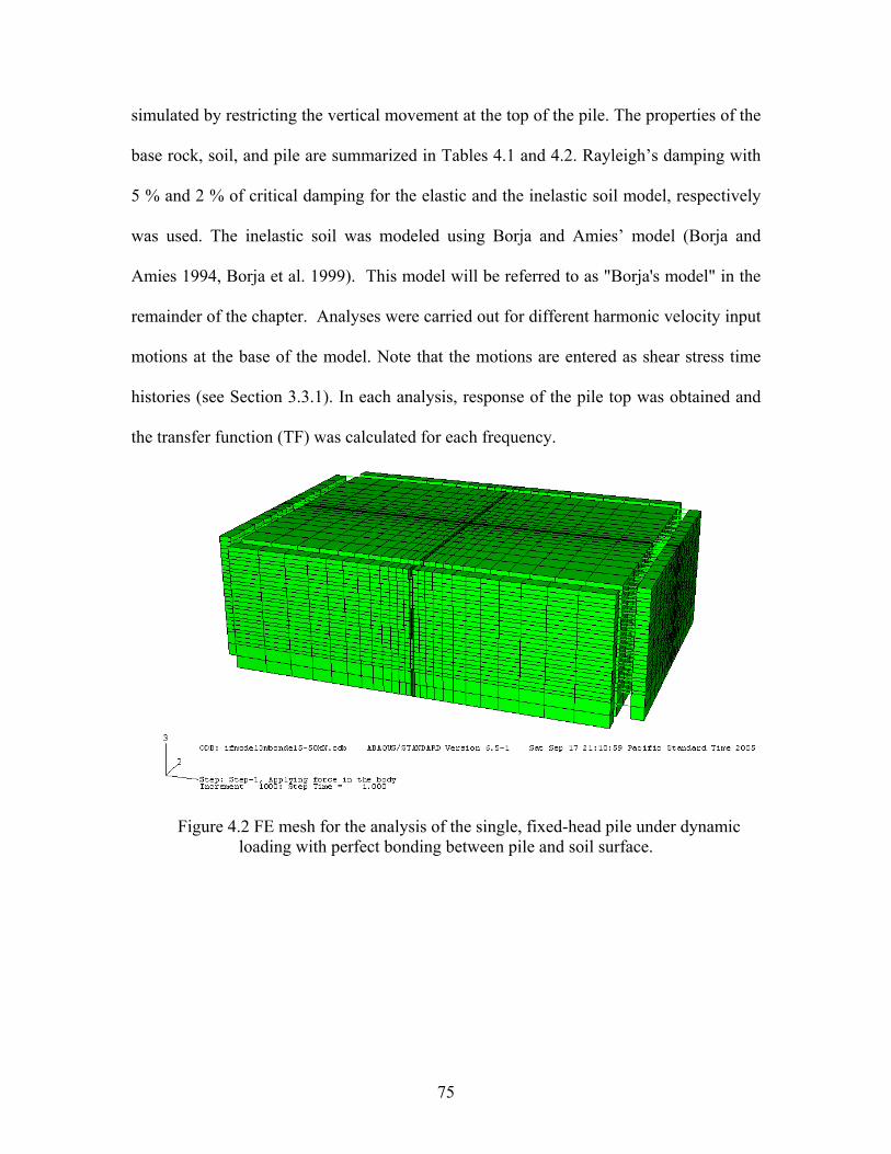
simulated by restricting the vertical movement at the top of the pile. The properties of the

base rock, soil, and pile are summarized in Tables 4.1 and 4.2. Rayleigh’s damping with

5 % and 2 % of critical damping for the elastic and the inelastic soil model, respectively

was used. The inelastic soil was modeled using Borja and Amies’ model (Borja and

Amies 1994, Borja et al. 1999). This model will be referred to as "Borja's model" in the

remainder of the chapter. Analyses were carried out for different harmonic velocity input

motions at the base of the model. Note that the motions are entered as shear stress time

histories (see Section 3.3.1). In each analysis, response of the pile top was obtained and

the transfer function (TF) was calculated for each frequency.

Figure 4.2 FE mesh for the analysis of the single, fixed-head pile under dynamic loading with perfect bonding between pile and soil surface.

75

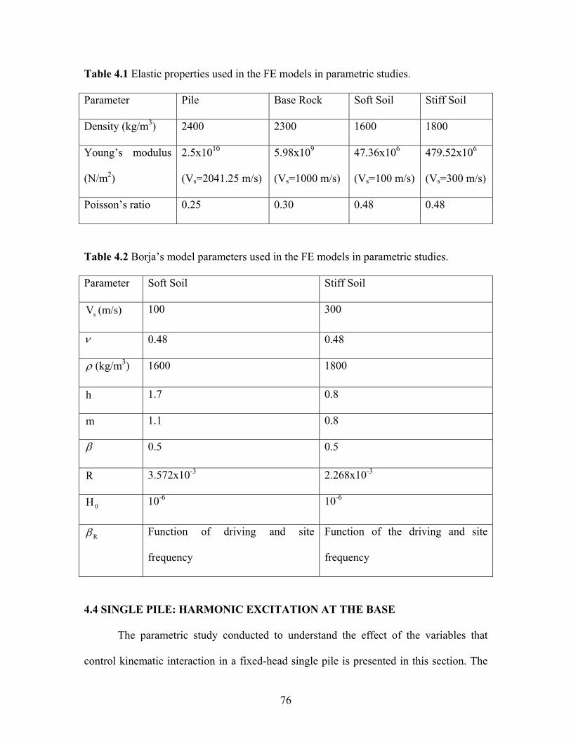
Table 4.1 Elastic properties used in the FE models in parametric studies.

Parameter Pile Base Rock Soft Soil Stiff Soil

Density (kg/m3) 2400 2300 1600 1800

Young’s modulus

(N/m2)

2.5x1010

(Vs=2041.25 m/s)

5.98x109

(Vs=1000 m/s)

47.36x106

(Vs=100 m/s)

479.52x106

(Vs=300 m/s)

Poisson’s ratio 0.25 0.30 0.48 0.48

Table 4.2 Borja’s model parameters used in the FE models in parametric studies.

Parameter Soft Soil Stiff Soil

sV (m/s) 100 300

ν 0.48 0.48

ρ (kg/m3) 1600 1800

h 1.7 0.8

m 1.1 0.8

β 0.5 0.5

R 3.572x10-3 2.268x10-3

0H 10-6 10-6

Rβ Function of driving and site

frequency

Function of the driving and site

frequency

4.4 SINGLE PILE: HARMONIC EXCITATION AT THE BASE

The parametric study conducted to understand the effect of the variables that

control kinematic interaction in a fixed-head single pile is presented in this section. The

76

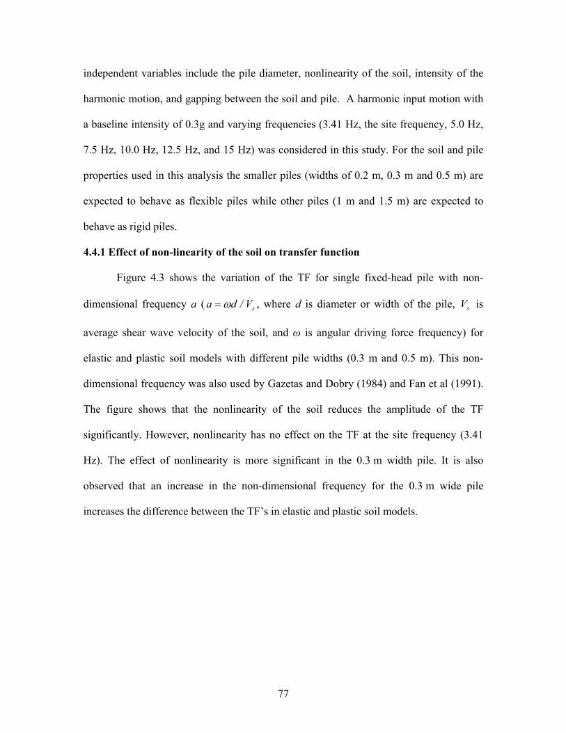
independent variables include the pile diameter, nonlinearity of the soil, intensity of the

harmonic motion, and gapping between the soil and pile. A harmonic input motion with

a baseline intensity of 0.3g and varying frequencies (3.41 Hz, the site frequency, 5.0 Hz,

7.5 Hz, 10.0 Hz, 12.5 Hz, and 15 Hz) was considered in this study. For the soil and pile

properties used in this analysis the smaller piles (widths of 0.2 m, 0.3 m and 0.5 m) are

expected to behave as flexible piles while other piles (1 m and 1.5 m) are expected to

behave as rigid piles.

4.4.1 Effect of non-linearity of the soil on transfer function

Figure 4.3 shows the variation of the TF for single fixed-head pile with non-

dimensional frequency a ( sV/da ω= , where d is diameter or width of the pile, is

average shear wave velocity of the soil, and ω is angular driving force frequency) for

elastic and plastic soil models with different pile widths (0.3 m and 0.5 m). This non-

dimensional frequency was also used by Gazetas and Dobry (1984) and Fan et al (1991).

The figure shows that the nonlinearity of the soil reduces the amplitude of the TF

significantly. However, nonlinearity has no effect on the TF at the site frequency (3.41

Hz). The effect of nonlinearity is more significant in the 0.3 m width pile. It is also

observed that an increase in the non-dimensional frequency for the 0.3 m wide pile

increases the difference between the TF’s in elastic and plastic soil models.

sV

77

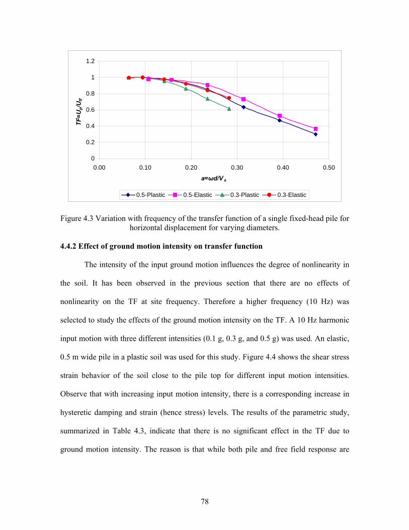
0

0.2

0.4

0.6

0.8

1

1.2

0.00 0.10 0.20 0.30 0.40 0.50

a=ωd/V s

TF=U

p/Uff

0.5-Plastic 0.5-Elastic 0.3-Plastic 0.3-Elastic

Figure 4.3 Variation with frequency of the transfer function of a single fixed-head pile for horizontal displacement for varying diameters.

4.4.2 Effect of ground motion intensity on transfer function

The intensity of the input ground motion influences the degree of nonlinearity in

the soil. It has been observed in the previous section that there are no effects of

nonlinearity on the TF at site frequency. Therefore a higher frequency (10 Hz) was

selected to study the effects of the ground motion intensity on the TF. A 10 Hz harmonic

input motion with three different intensities (0.1 g, 0.3 g, and 0.5 g) was used. An elastic,

0.5 m wide pile in a plastic soil was used for this study. Figure 4.4 shows the shear stress

strain behavior of the soil close to the pile top for different input motion intensities.

Observe that with increasing input motion intensity, there is a corresponding increase in

hysteretic damping and strain (hence stress) levels. The results of the parametric study,

summarized in Table 4.3, indicate that there is no significant effect in the TF due to

ground motion intensity. The reason is that while both pile and free field response are

78

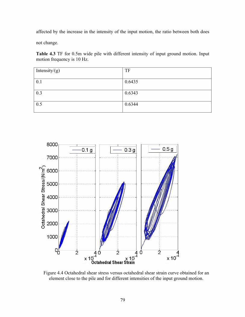
affected by the increase in the intensity of the input motion, the ratio between both does

not change.

Table 4.3 TF for 0.5m wide pile with different intensity of input ground motion. Input motion frequency is 10 Hz. Intensity/(g) TF

0.1 0.6435

0.3 0.6343

0.5 0.6344

Figure 4.4 Octahedral shear stress versus octahedral shear strain curve obtained for an element close to the pile and for different intensities of the input ground motion.

79

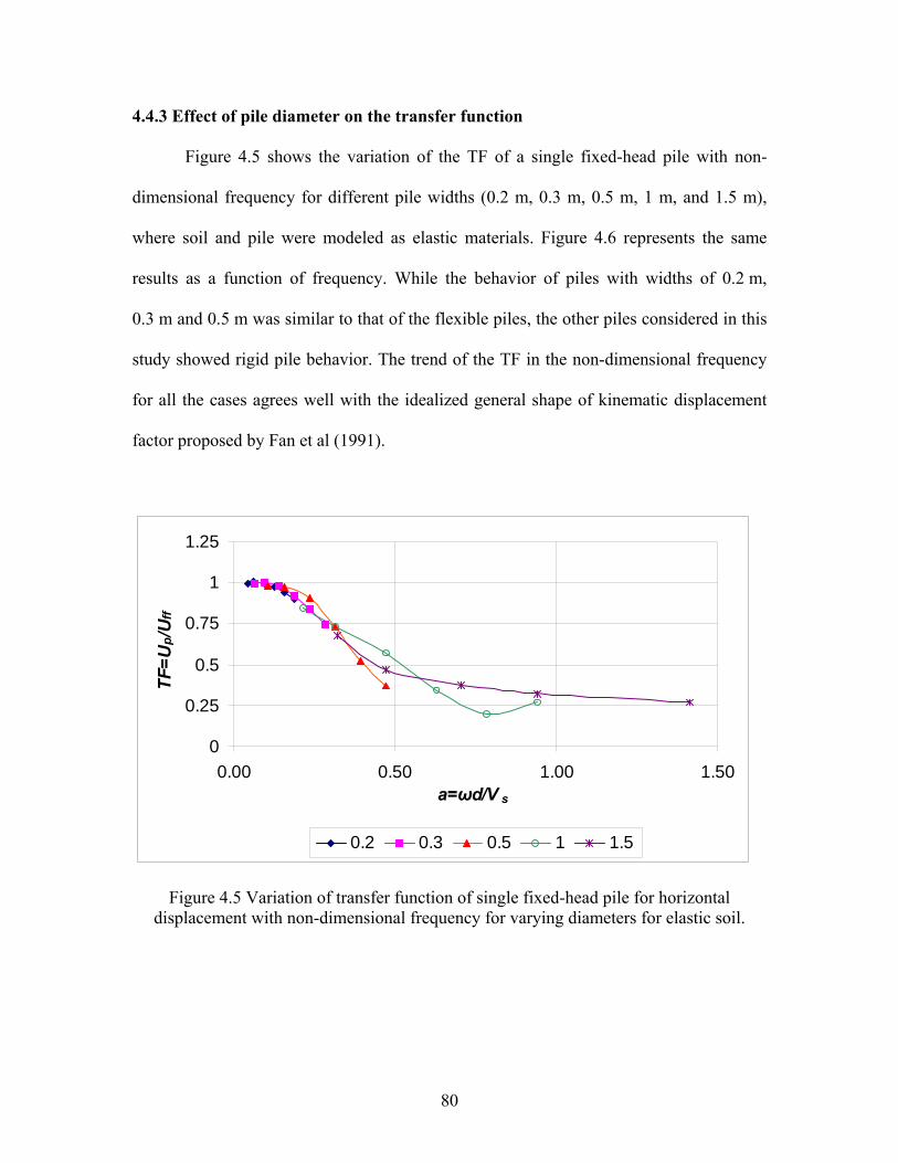
4.4.3 Effect of pile diameter on the transfer function

Figure 4.5 shows the variation of the TF of a single fixed-head pile with non-

dimensional frequency for different pile widths (0.2 m, 0.3 m, 0.5 m, 1 m, and 1.5 m),

where soil and pile were modeled as elastic materials. Figure 4.6 represents the same

results as a function of frequency. While the behavior of piles with widths of 0.2 m,

0.3 m and 0.5 m was similar to that of the flexible piles, the other piles considered in this

study showed rigid pile behavior. The trend of the TF in the non-dimensional frequency

for all the cases agrees well with the idealized general shape of kinematic displacement

factor proposed by Fan et al (1991).

0

0.25

0.5

0.75

1

1.25

0.00 0.50 1.00 1.50a=ωd/V s

TF=U

p/Uff

0.2 0.3 0.5 1 1.5

Figure 4.5 Variation of transfer function of single fixed-head pile for horizontal displacement with non-dimensional frequency for varying diameters for elastic soil.

80

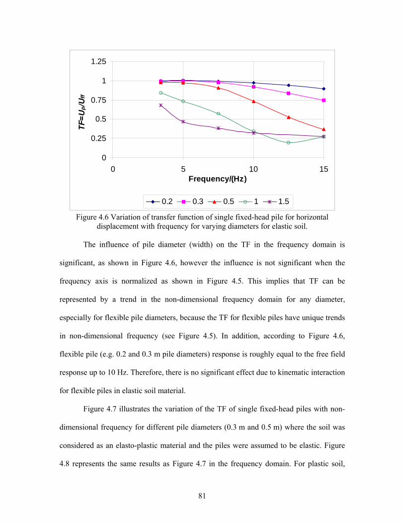
0

0.25

0.5

0.75

1

1.25

0 5 10 15Frequency/(Hz)

TF=U

p/Uff

0.2 0.3 0.5 1 1.5

Figure 4.6 Variation of transfer function of single fixed-head pile for horizontal displacement with frequency for varying diameters for elastic soil.

The influence of pile diameter (width) on the TF in the frequency domain is

significant, as shown in Figure 4.6, however the influence is not significant when the

frequency axis is normalized as shown in Figure 4.5. This implies that TF can be

represented by a trend in the non-dimensional frequency domain for any diameter,

especially for flexible pile diameters, because the TF for flexible piles have unique trends

in non-dimensional frequency (see Figure 4.5). In addition, according to Figure 4.6,

flexible pile (e.g. 0.2 and 0.3 m pile diameters) response is roughly equal to the free field

response up to 10 Hz. Therefore, there is no significant effect due to kinematic interaction

for flexible piles in elastic soil material.

Figure 4.7 illustrates the variation of the TF of single fixed-head piles with non-

dimensional frequency for different pile diameters (0.3 m and 0.5 m) where the soil was

considered as an elasto-plastic material and the piles were assumed to be elastic. Figure

4.8 represents the same results as Figure 4.7 in the frequency domain. For plastic soil,

81

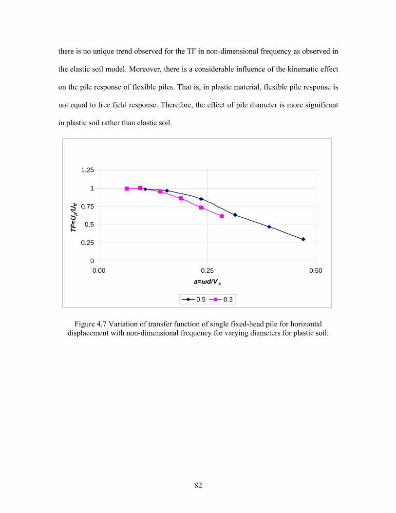
there is no unique trend observed for the TF in non-dimensional frequency as observed in

the elastic soil model. Moreover, there is a considerable influence of the kinematic effect

on the pile response of flexible piles. That is, in plastic material, flexible pile response is

not equal to free field response. Therefore, the effect of pile diameter is more significant

in plastic soil rather than elastic soil.

0

0.25

0.5

0.75

1

1.25

0.00 0.25 0.50a=ωd/V s

TF=U

p/Uff

0.5 0.3

Figure 4.7 Variation of transfer function of single fixed-head pile for horizontal displacement with non-dimensional frequency for varying diameters for plastic soil.

82

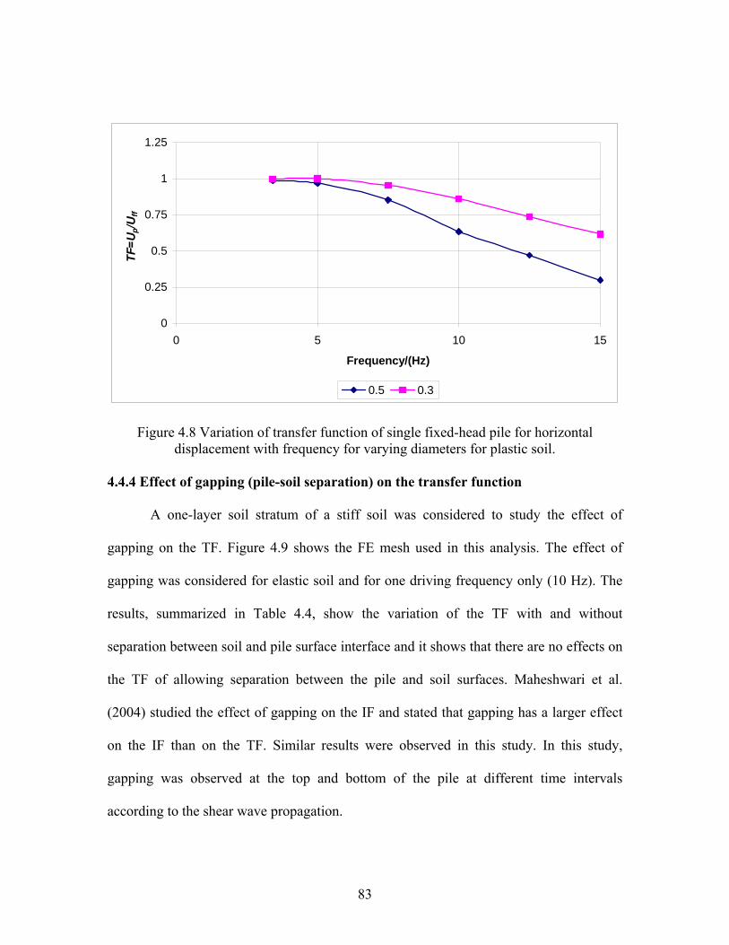
0

0.25

0.5

0.75

1

1.25

0 5 10 15

Frequency/(Hz)

TF=U

p/Uff

0.5 0.3

Figure 4.8 Variation of transfer function of single fixed-head pile for horizontal displacement with frequency for varying diameters for plastic soil.

4.4.4 Effect of gapping (pile-soil separation) on the transfer function

A one-layer soil stratum of a stiff soil was considered to study the effect of

gapping on the TF. Figure 4.9 shows the FE mesh used in this analysis. The effect of

gapping was considered for elastic soil and for one driving frequency only (10 Hz). The

results, summarized in Table 4.4, show the variation of the TF with and without

separation between soil and pile surface interface and it shows that there are no effects on

the TF of allowing separation between the pile and soil surfaces. Maheshwari et al.

(2004) studied the effect of gapping on the IF and stated that gapping has a larger effect

on the IF than on the TF. Similar results were observed in this study. In this study,

gapping was observed at the top and bottom of the pile at different time intervals

according to the shear wave propagation.

83

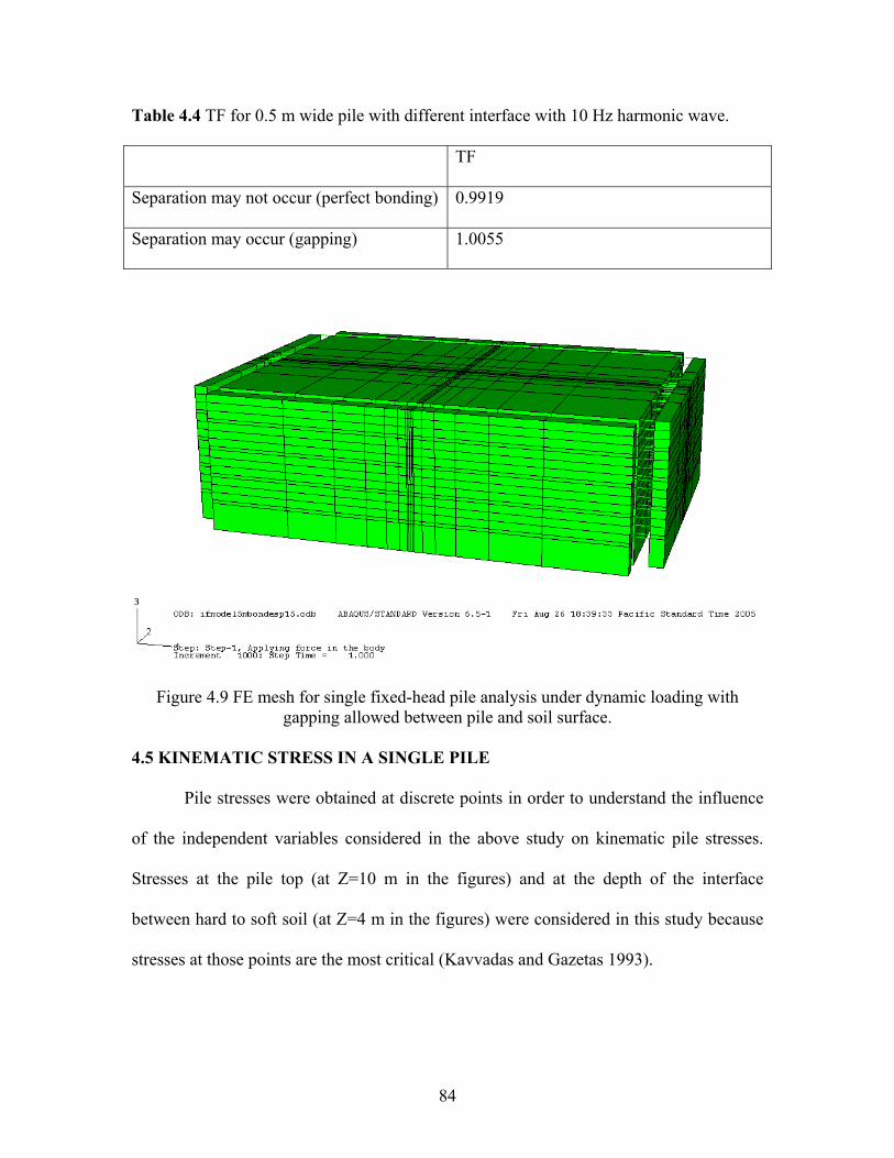
Table 4.4 TF for 0.5 m wide pile with different interface with 10 Hz harmonic wave.

TF

Separation may not occur (perfect bonding) 0.9919

Separation may occur (gapping) 1.0055

Figure 4.9 FE mesh for single fixed-head pile analysis under dynamic loading with gapping allowed between pile and soil surface.

4.5 KINEMATIC STRESS IN A SINGLE PILE

Pile stresses were obtained at discrete points in order to understand the influence

of the independent variables considered in the above study on kinematic pile stresses.

Stresses at the pile top (at Z=10 m in the figures) and at the depth of the interface

between hard to soft soil (at Z=4 m in the figures) were considered in this study because

stresses at those points are the most critical (Kavvadas and Gazetas 1993).

84

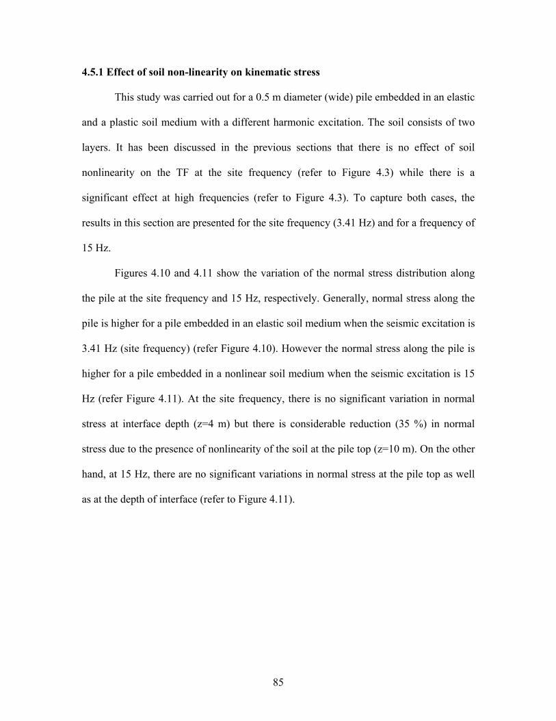
4.5.1 Effect of soil non-linearity on kinematic stress

This study was carried out for a 0.5 m diameter (wide) pile embedded in an elastic

and a plastic soil medium with a different harmonic excitation. The soil consists of two

layers. It has been discussed in the previous sections that there is no effect of soil

nonlinearity on the TF at the site frequency (refer to Figure 4.3) while there is a

significant effect at high frequencies (refer to Figure 4.3). To capture both cases, the

results in this section are presented for the site frequency (3.41 Hz) and for a frequency of

15 Hz.

Figures 4.10 and 4.11 show the variation of the normal stress distribution along

the pile at the site frequency and 15 Hz, respectively. Generally, normal stress along the

pile is higher for a pile embedded in an elastic soil medium when the seismic excitation is

3.41 Hz (site frequency) (refer Figure 4.10). However the normal stress along the pile is

higher for a pile embedded in a nonlinear soil medium when the seismic excitation is 15

Hz (refer Figure 4.11). At the site frequency, there is no significant variation in normal

stress at interface depth (z=4 m) but there is considerable reduction (35 %) in normal

stress due to the presence of nonlinearity of the soil at the pile top (z=10 m). On the other

hand, at 15 Hz, there are no significant variations in normal stress at the pile top as well

as at the depth of interface (refer to Figure 4.11).

85

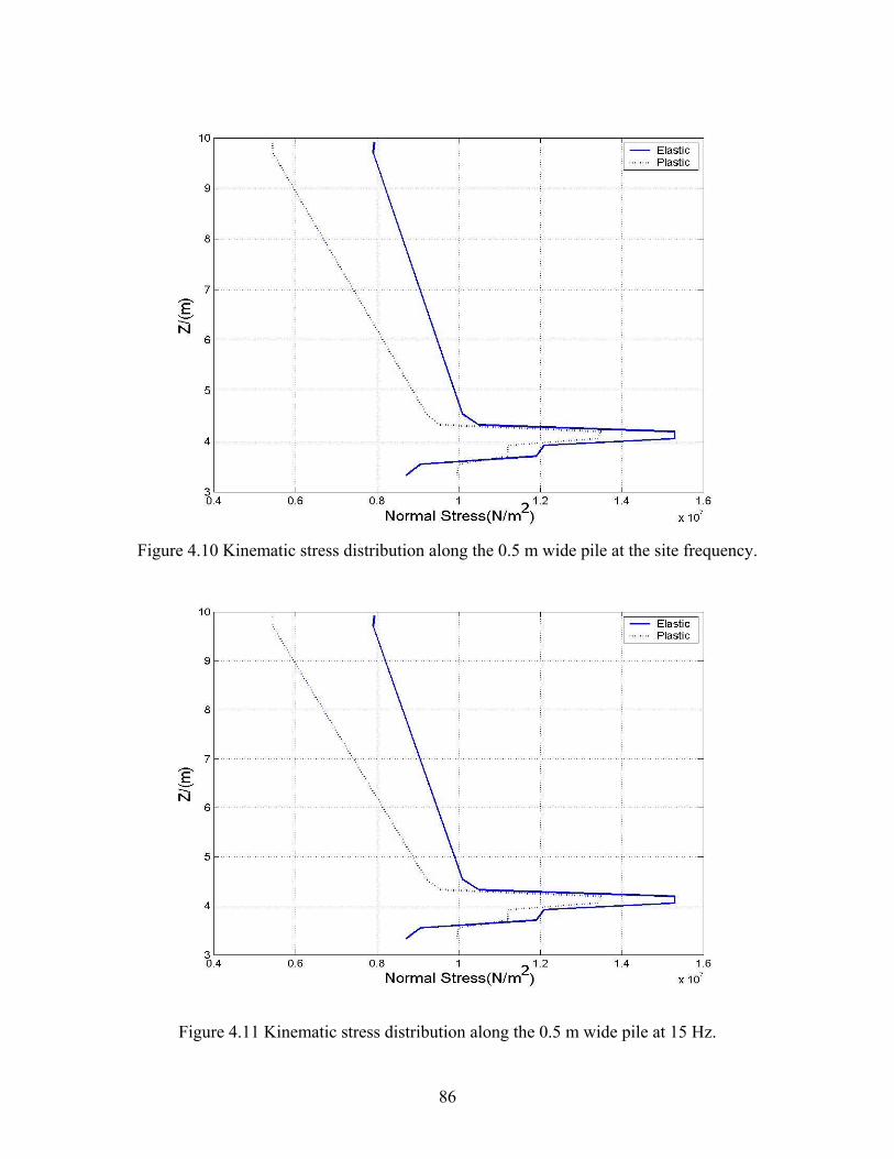
Figure 4.10 Kinematic stress distribution along the 0.5 m wide pile at the site frequency.

Figure 4.11 Kinematic stress distribution along the 0.5 m wide pile at 15 Hz.

86

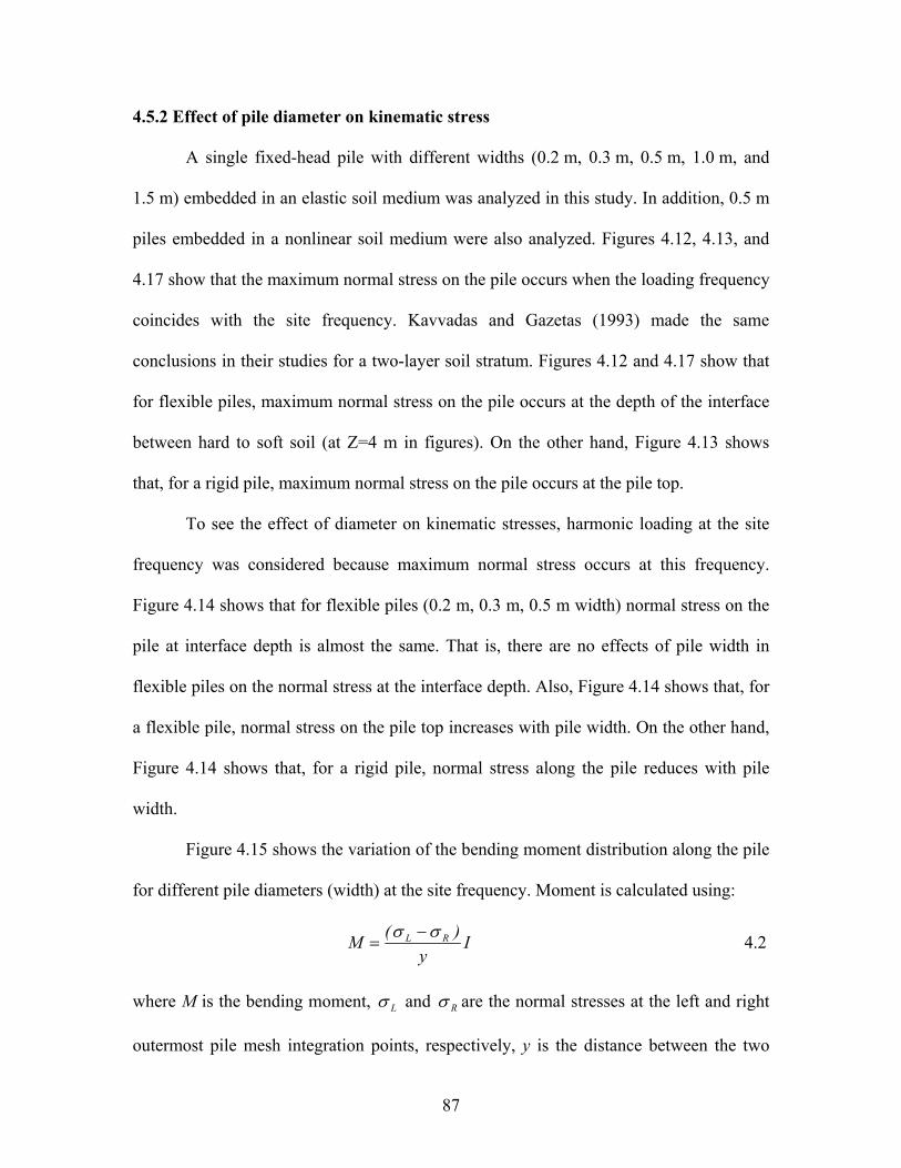
4.5.2 Effect of pile diameter on kinematic stress

A single fixed-head pile with different widths (0.2 m, 0.3 m, 0.5 m, 1.0 m, and

1.5 m) embedded in an elastic soil medium was analyzed in this study. In addition, 0.5 m

piles embedded in a nonlinear soil medium were also analyzed. Figures 4.12, 4.13, and

4.17 show that the maximum normal stress on the pile occurs when the loading frequency

coincides with the site frequency. Kavvadas and Gazetas (1993) made the same

conclusions in their studies for a two-layer soil stratum. Figures 4.12 and 4.17 show that

for flexible piles, maximum normal stress on the pile occurs at the depth of the interface

between hard to soft soil (at Z=4 m in figures). On the other hand, Figure 4.13 shows

that, for a rigid pile, maximum normal stress on the pile occurs at the pile top.

To see the effect of diameter on kinematic stresses, harmonic loading at the site

frequency was considered because maximum normal stress occurs at this frequency.

Figure 4.14 shows that for flexible piles (0.2 m, 0.3 m, 0.5 m width) normal stress on the

pile at interface depth is almost the same. That is, there are no effects of pile width in

flexible piles on the normal stress at the interface depth. Also, Figure 4.14 shows that, for

a flexible pile, normal stress on the pile top increases with pile width. On the other hand,

Figure 4.14 shows that, for a rigid pile, normal stress along the pile reduces with pile

width.

Figure 4.15 shows the variation of the bending moment distribution along the pile

for different pile diameters (width) at the site frequency. Moment is calculated using:

Iy

)(M RL σσ −= 4.2

where M is the bending moment, Lσ and Rσ are the normal stresses at the left and right

outermost pile mesh integration points, respectively, y is the distance between the two

87

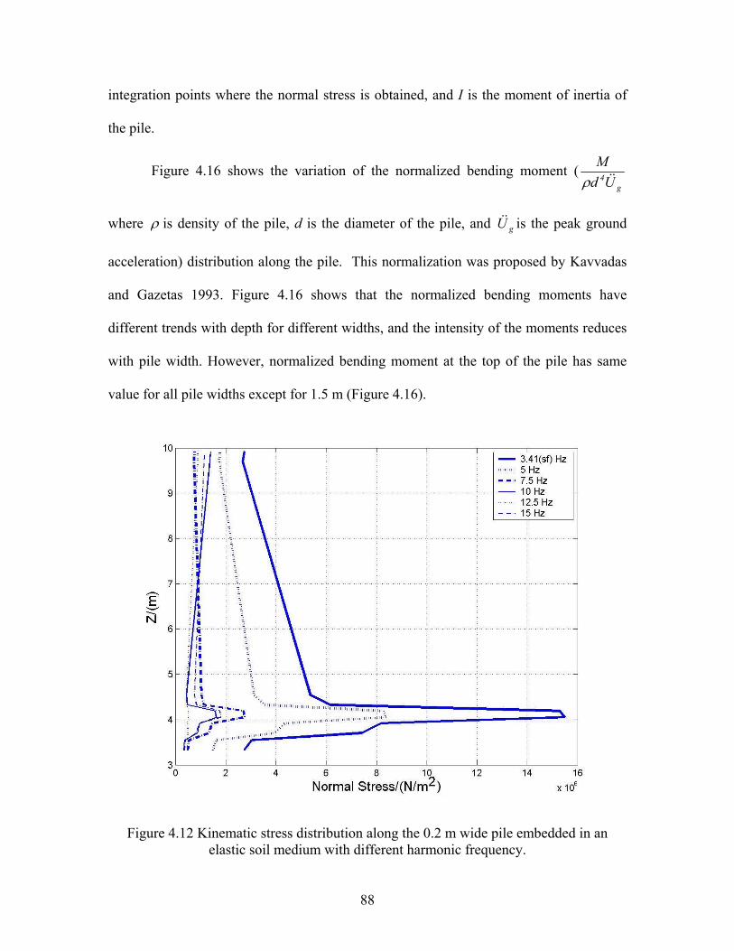
integration points where the normal stress is obtained, and I is the moment of inertia of

the pile.

Figure 4.16 shows the variation of the normalized bending moment (g

4UdM&&ρ

where ρ is density of the pile, d is the diameter of the pile, and is the peak ground

acceleration) distribution along the pile. This normalization was proposed by Kavvadas

and Gazetas 1993. Figure 4.16 shows that the normalized bending moments have

different trends with depth for different widths, and the intensity of the moments reduces

with pile width. However, normalized bending moment at the top of the pile has same

value for all pile widths except for 1.5 m (Figure 4.16).

gU&&

Figure 4.12 Kinematic stress distribution along the 0.2 m wide pile embedded in an elastic soil medium with different harmonic frequency.

88

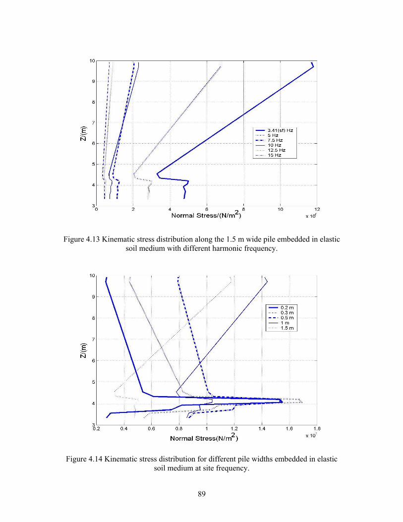
Figure 4.13 Kinematic stress distribution along the 1.5 m wide pile embedded in elastic soil medium with different harmonic frequency.

Figure 4.14 Kinematic stress distribution for different pile widths embedded in elastic soil medium at site frequency.

89

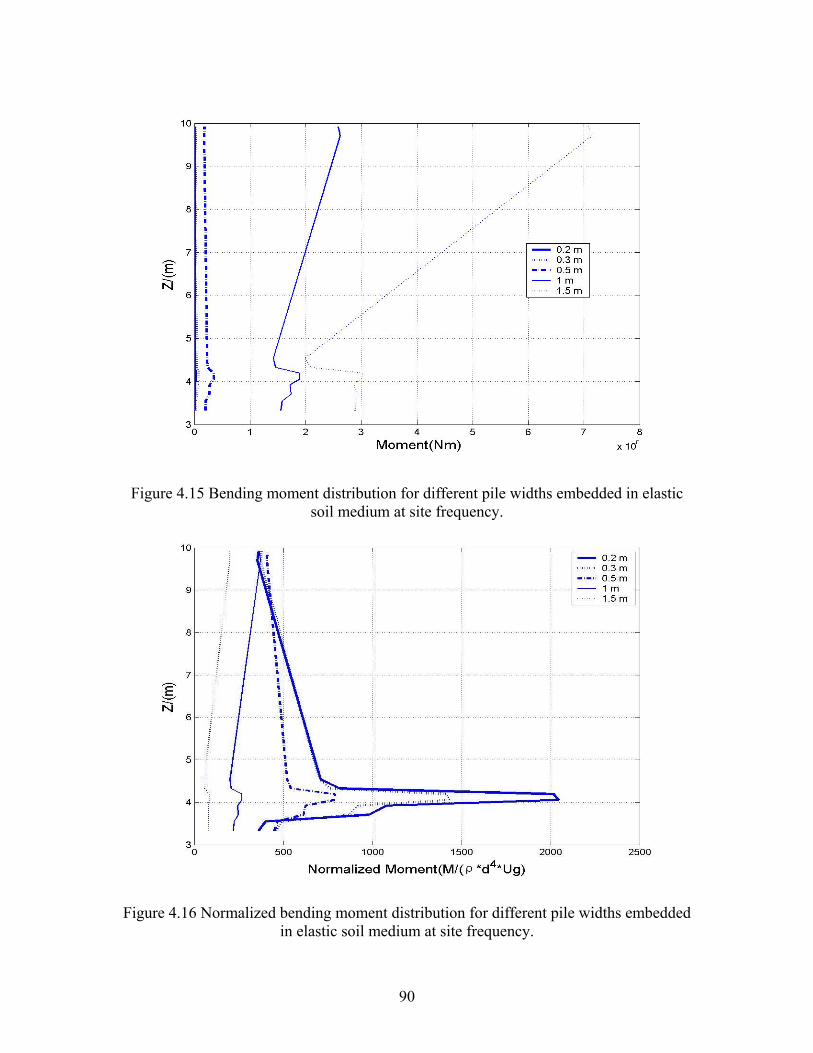
Figure 4.15 Bending moment distribution for different pile widths embedded in elastic soil medium at site frequency.

Figure 4.16 Normalized bending moment distribution for different pile widths embedded in elastic soil medium at site frequency.

90

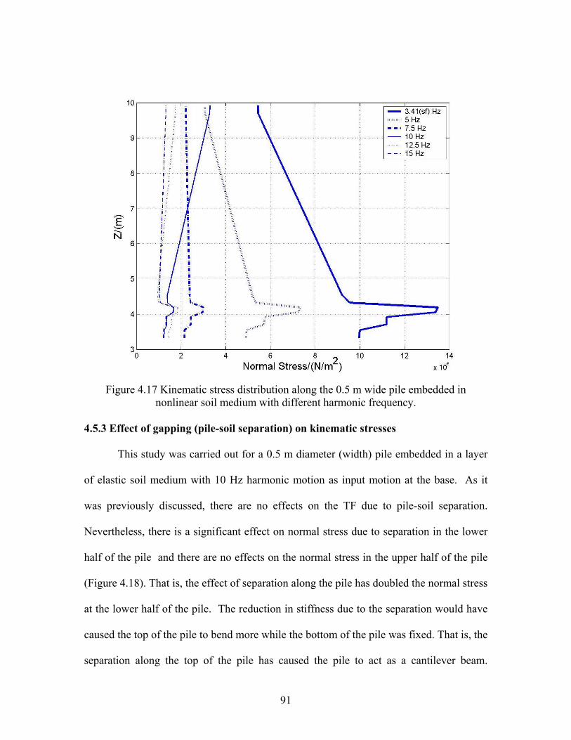
Figure 4.17 Kinematic stress distribution along the 0.5 m wide pile embedded in

nonlinear soil medium with different harmonic frequency.

4.5.3 Effect of gapping (pile-soil separation) on kinematic stresses

This study was carried out for a 0.5 m diameter (width) pile embedded in a layer

of elastic soil medium with 10 Hz harmonic motion as input motion at the base. As it

was previously discussed, there are no effects on the TF due to pile-soil separation.

Nevertheless, there is a significant effect on normal stress due to separation in the lower

half of the pile and there are no effects on the normal stress in the upper half of the pile

(Figure 4.18). That is, the effect of separation along the pile has doubled the normal stress

at the lower half of the pile. The reduction in stiffness due to the separation would have

caused the top of the pile to bend more while the bottom of the pile was fixed. That is, the

separation along the top of the pile has caused the pile to act as a cantilever beam.

91

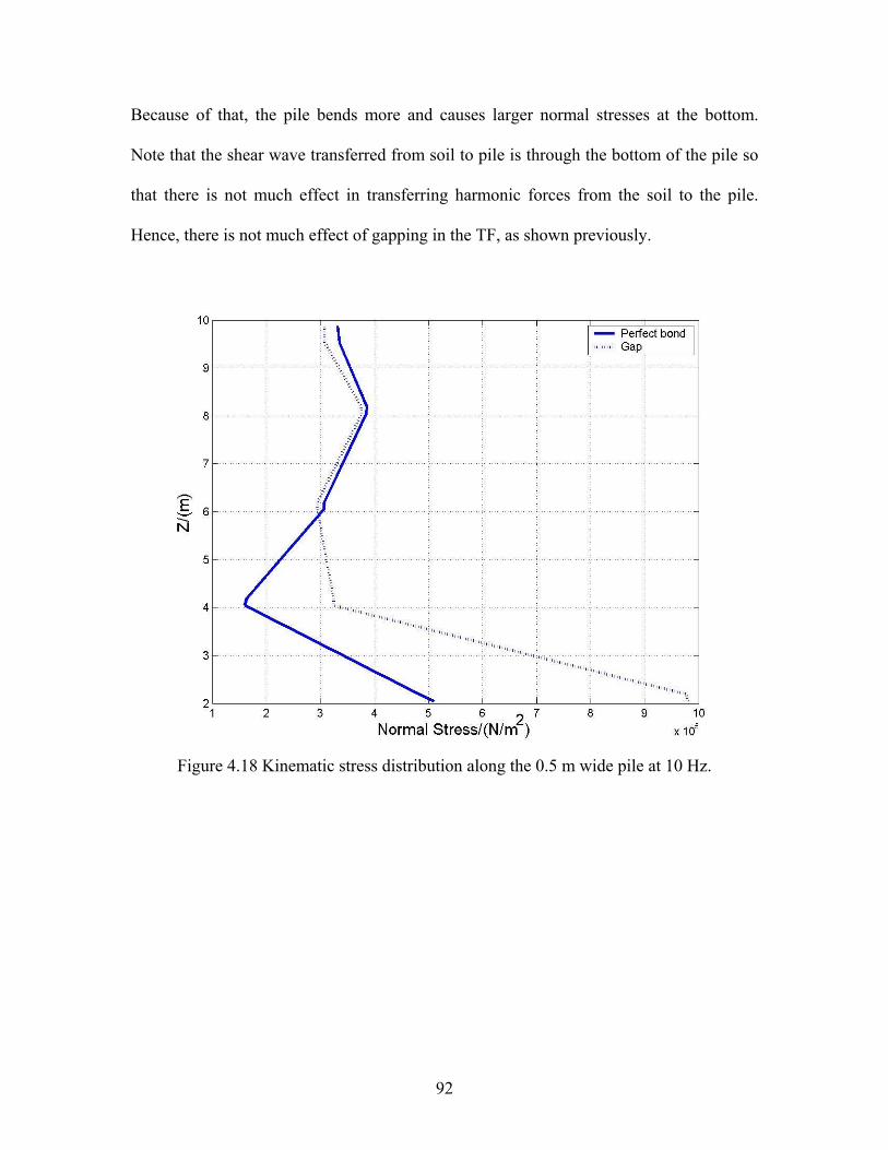
Because of that, the pile bends more and causes larger normal stresses at the bottom.

Note that the shear wave transferred from soil to pile is through the bottom of the pile so

that there is not much effect in transferring harmonic forces from the soil to the pile.

Hence, there is not much effect of gapping in the TF, as shown previously.

Figure 4.18 Kinematic stress distribution along the 0.5 m wide pile at 10 Hz.

92

CHAPTER 5

PARAMETRIC STUDY ON INERTIAL INTERACTION

5.1 INTRODUCTION

A parametric study was conducted in order to understand the effect of several

variables on the inertial interaction of a fixed-head single pile. In this study, the effects of

pile diameter, soil non-linearity, gapping, and magnitude of the driving force were

considered. The effect of these variables on the impedance function (see Section 2.2.1) is

studied. In addition, the effects of these variables on the inertial stresses in a fixed-head

single pile are also considered. The results of the parametric study will provide a better

understanding of the effects of inertial interaction on the dynamic behavior of a fixed-

head single pile.

5.2 COMPUTATION OF THE IMPEDANCE FUNCTION

The impedance function (dynamic stiffness) of the pile is required to calculate the

response of a structure to dynamic loading. The impedance function (IF) of a pile system

is defined by means of the stiffness and damping of the system. The IF can be

represented by a complex number in the frequency domain, and it is a function of the

driving frequency (e.g. the frequency of the loading function) and the magnitude of the

driving force, in addition to being a function of the properties of the soil-pile system. The

following equations were used in this study to calculate the impedance function (for

further details refer to Maheshwari et al. 2004):

5.1 θi00 e)U/P(IF =

ll tft πωθ 2== 5.2

93

where is the amplitude of the exciting lateral force applied at the top of the pile, is

the lateral peak amplitude response at the top of the pile at the steady state, is the time

lag between driving force and pile top response, and f is the driving frequency. In this

study, dynamic impedance functions were normalized with respect to static impedance

functions.

0P 0U

lt

5.3 MODEL DESCRIPTION

A similar FE model as the one described in section 4.3, but with different

boundary conditions, was used for this parametric study. The soil column was assumed to

be fixed in all directions, which implies that the lateral boundaries become absorbing

boundaries. The soil and pile properties used in this study are also identical to those

discussed in section 4.3. Analyses were carried out for varying harmonic driving forces at

the top of the pile. The response of the top of the pile was obtained and the impedance

function (IF) was calculated for varying frequencies.

5.4 SINGLE PILE: HARMONIC EXCITATION AT THE TOP OF THE PILE

The parametric study conducted to understand the effect of inertial interaction on

a single pile is presented in this section. The independent variables considered include the

pile diameter, soil nonlinearity, the magnitude of the driving force, and gapping between

the soil and pile. The baseline magnitude of the driving forces was selected as the

magnitude of a static force that would cause a pile top deflection of 25 mm. This force

was considered an ultimate load, and was obtained through an analysis using the software

LPILE. The results of the LPILE analysis are summarized in Table 5.1. Various loading

frequencies (3.41 Hz, the site frequency, 5.0 Hz, 7.5 Hz, 10.0 Hz, 12.5 Hz., and 15 Hz)

were considered for this study.

94

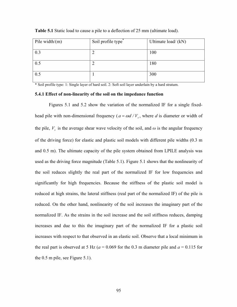
Table 5.1 Static load to cause a pile to a deflection of 25 mm (ultimate load).

Pile width/(m) Soil profile type* Ultimate load/ (kN)

0.3 2 100

0.5 2 180

0.5 1 300

* Soil profile type: 1: Single layer of hard soil. 2: Soft soil layer underlain by a hard stratum. 5.4.1 Effect of non-linearity of the soil on the impedance function

Figures 5.1 and 5.2 show the variation of the normalized IF for a single fixed-

head pile with non-dimensional frequency ( sV/da ω= , where d is diameter or width of

the pile, is the average shear wave velocity of the soil, and ω is the angular frequency

of the driving force) for elastic and plastic soil models with different pile widths (0.3 m

and 0.5 m). The ultimate capacity of the pile system obtained from LPILE analysis was

used as the driving force magnitude (Table 5.1). Figure 5.1 shows that the nonlinearity of

the soil reduces slightly the real part of the normalized IF for low frequencies and

significantly for high frequencies. Because the stiffness of the plastic soil model is

reduced at high strains, the lateral stiffness (real part of the normalized IF) of the pile is

reduced. On the other hand, nonlinearity of the soil increases the imaginary part of the

normalized IF. As the strains in the soil increase and the soil stiffness reduces, damping

increases and due to this the imaginary part of the normalized IF for a plastic soil

increases with respect to that observed in an elastic soil. Observe that a local minimum in

the real part is observed at 5 Hz (a = 0.069 for the 0.3 m diameter pile and a = 0.115 for

the 0.5 m pile, see Figure 5.1).

sV

95

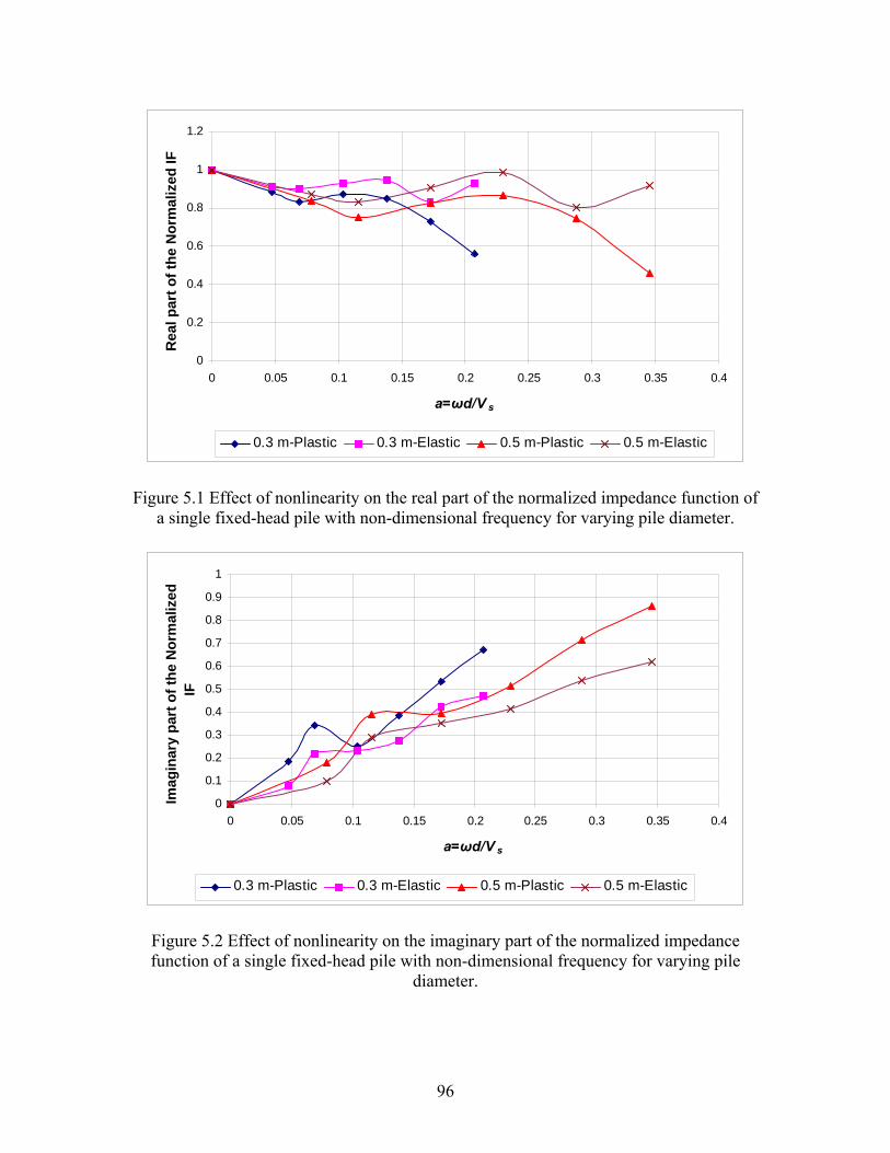
0

0.2

0.4

0.6

0.8

1

1.2

0 0.05 0.1 0.15 0.2 0.25 0.3 0.35 0.4

a=ωd/V s

Rea

l par

t of t

he N

orm

aliz

ed IF

0.3 m-Plastic 0.3 m-Elastic 0.5 m-Plastic 0.5 m-Elastic

Figure 5.1 Effect of nonlinearity on the real part of the normalized impedance function of a single fixed-head pile with non-dimensional frequency for varying pile diameter.

0

0.1

0.2

0.3

0.4

0.5

0.6

0.7

0.8

0.9

1

0 0.05 0.1 0.15 0.2 0.25 0.3 0.35 0.4

a=ωd/V s

Imag

inar

y pa

rt o

f the

Nor

mal

ized

IF

0.3 m-Plastic 0.3 m-Elastic 0.5 m-Plastic 0.5 m-Elastic

Figure 5.2 Effect of nonlinearity on the imaginary part of the normalized impedance function of a single fixed-head pile with non-dimensional frequency for varying pile

diameter.

96

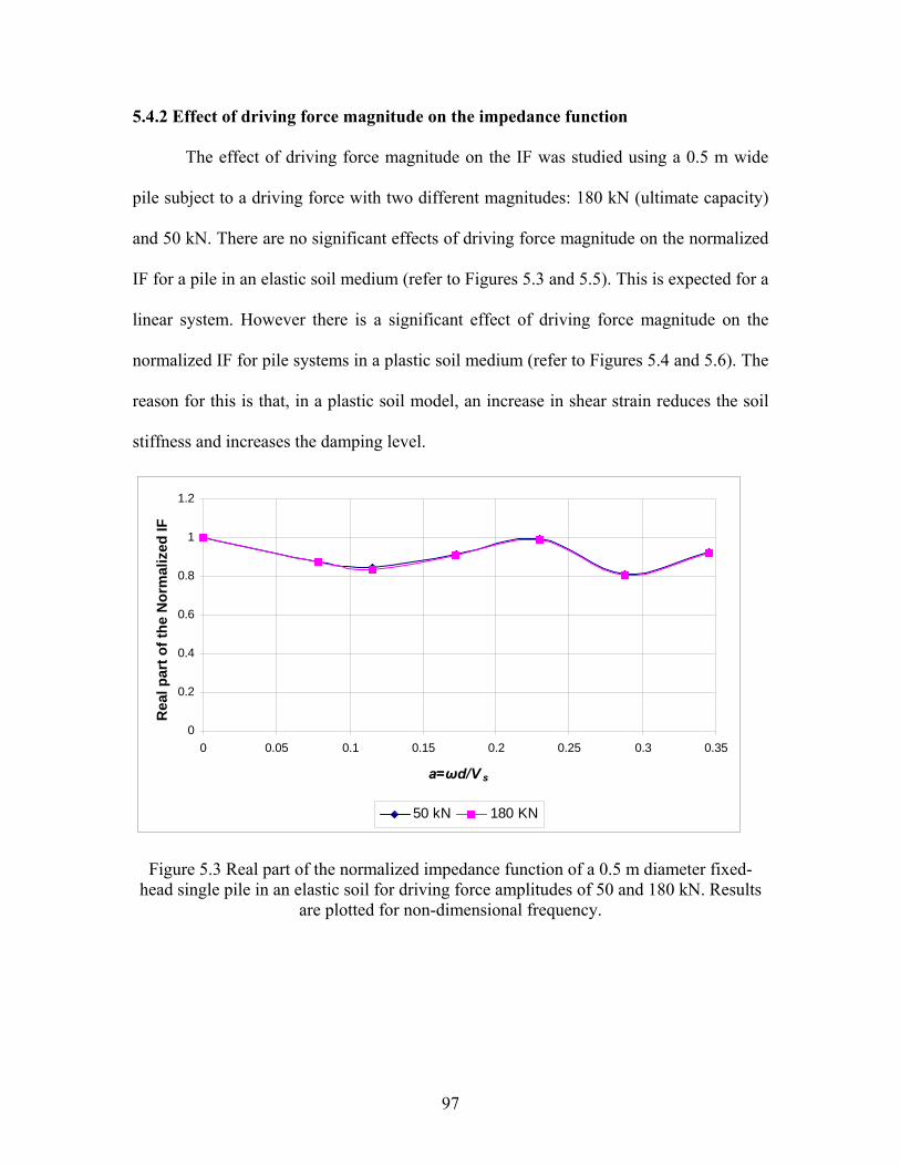
5.4.2 Effect of driving force magnitude on the impedance function

The effect of driving force magnitude on the IF was studied using a 0.5 m wide

pile subject to a driving force with two different magnitudes: 180 kN (ultimate capacity)

and 50 kN. There are no significant effects of driving force magnitude on the normalized

IF for a pile in an elastic soil medium (refer to Figures 5.3 and 5.5). This is expected for a

linear system. However there is a significant effect of driving force magnitude on the

normalized IF for pile systems in a plastic soil medium (refer to Figures 5.4 and 5.6). The

reason for this is that, in a plastic soil model, an increase in shear strain reduces the soil

stiffness and increases the damping level.

0

0.2

0.4

0.6

0.8

1

1.2

0 0.05 0.1 0.15 0.2 0.25 0.3 0.35

a=ωd/V s

Rea

l par

t of t

he N

orm

aliz

ed IF

50 kN 180 KN

Figure 5.3 Real part of the normalized impedance function of a 0.5 m diameter fixed-head single pile in an elastic soil for driving force amplitudes of 50 and 180 kN. Results

are plotted for non-dimensional frequency.

97

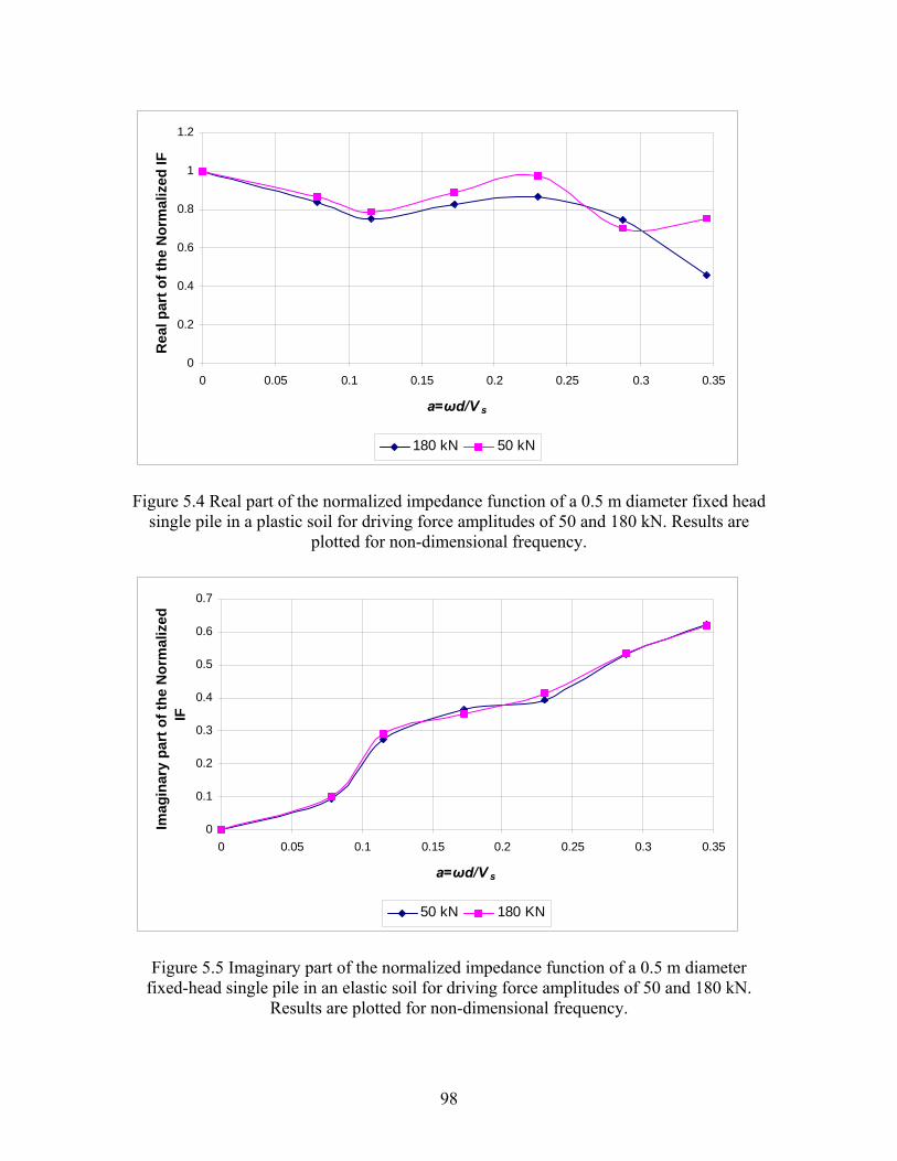
0

0.2

0.4

0.6

0.8

1

1.2

0 0.05 0.1 0.15 0.2 0.25 0.3 0.35

a=ωd/V s

Rea

l par

t of t

he N

orm

aliz

ed IF

180 kN 50 kN

Figure 5.4 Real part of the normalized impedance function of a 0.5 m diameter fixed head single pile in a plastic soil for driving force amplitudes of 50 and 180 kN. Results are

plotted for non-dimensional frequency.

0

0.1

0.2

0.3

0.4

0.5

0.6

0.7

0 0.05 0.1 0.15 0.2 0.25 0.3 0.35

a=ωd/V s

Imag

inar

y pa

rt o

f the

Nor

mal

ized

IF

50 kN 180 KN

Figure 5.5 Imaginary part of the normalized impedance function of a 0.5 m diameter fixed-head single pile in an elastic soil for driving force amplitudes of 50 and 180 kN.

Results are plotted for non-dimensional frequency.

98

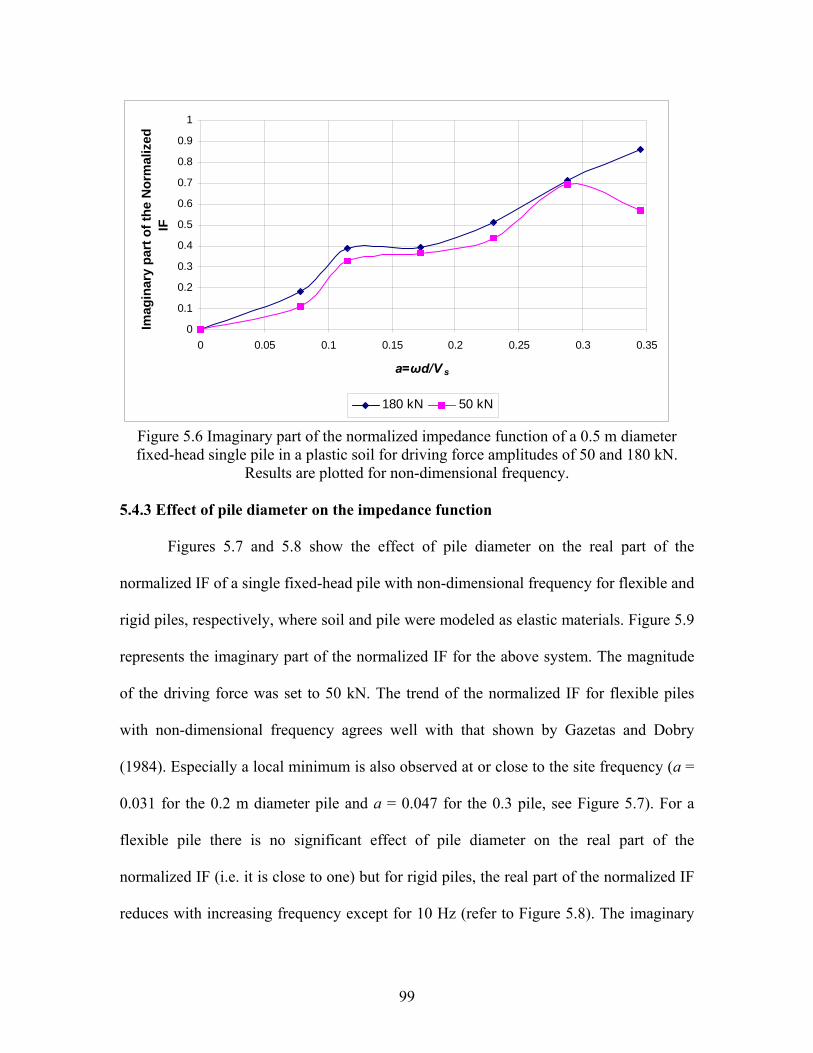
0

0.1

0.2

0.3

0.4

0.5

0.6

0.7

0.8

0.9

1

0 0.05 0.1 0.15 0.2 0.25 0.3 0.35

a=ωd/V s

Imag

inar

y pa

rt o

f the

Nor

mal

ized

IF

180 kN 50 kN

Figure 5.6 Imaginary part of the normalized impedance function of a 0.5 m diameter fixed-head single pile in a plastic soil for driving force amplitudes of 50 and 180 kN.

Results are plotted for non-dimensional frequency. 5.4.3 Effect of pile diameter on the impedance function

Figures 5.7 and 5.8 show the effect of pile diameter on the real part of the

normalized IF of a single fixed-head pile with non-dimensional frequency for flexible and

rigid piles, respectively, where soil and pile were modeled as elastic materials. Figure 5.9

represents the imaginary part of the normalized IF for the above system. The magnitude

of the driving force was set to 50 kN. The trend of the normalized IF for flexible piles

with non-dimensional frequency agrees well with that shown by Gazetas and Dobry

(1984). Especially a local minimum is also observed at or close to the site frequency (a =

0.031 for the 0.2 m diameter pile and a = 0.047 for the 0.3 pile, see Figure 5.7). For a

flexible pile there is no significant effect of pile diameter on the real part of the

normalized IF (i.e. it is close to one) but for rigid piles, the real part of the normalized IF

reduces with increasing frequency except for 10 Hz (refer to Figure 5.8). The imaginary

99

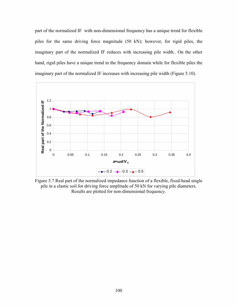
part of the normalized IF with non-dimensional frequency has a unique trend for flexible

piles for the same driving force magnitude (50 kN); however, for rigid piles, the

imaginary part of the normalized IF reduces with increasing pile width.. On the other

hand, rigid piles have a unique trend in the frequency domain while for flexible piles the

imaginary part of the normalized IF increases with increasing pile width (Figure 5.10).

0

0.2

0.4

0.6

0.8

1

1.2

0 0.05 0.1 0.15 0.2 0.25 0.3 0.35 0.4

a=ωd/V s

Rea

l par

t of t

he N

orm

aliz

ed IF

0.2 0.3 0.5

Figure 5.7 Real part of the normalized impedance function of a flexible, fixed-head single pile in a elastic soil for driving force amplitude of 50 kN for varying pile diameters.

Results are plotted for non-dimensional frequency.

100

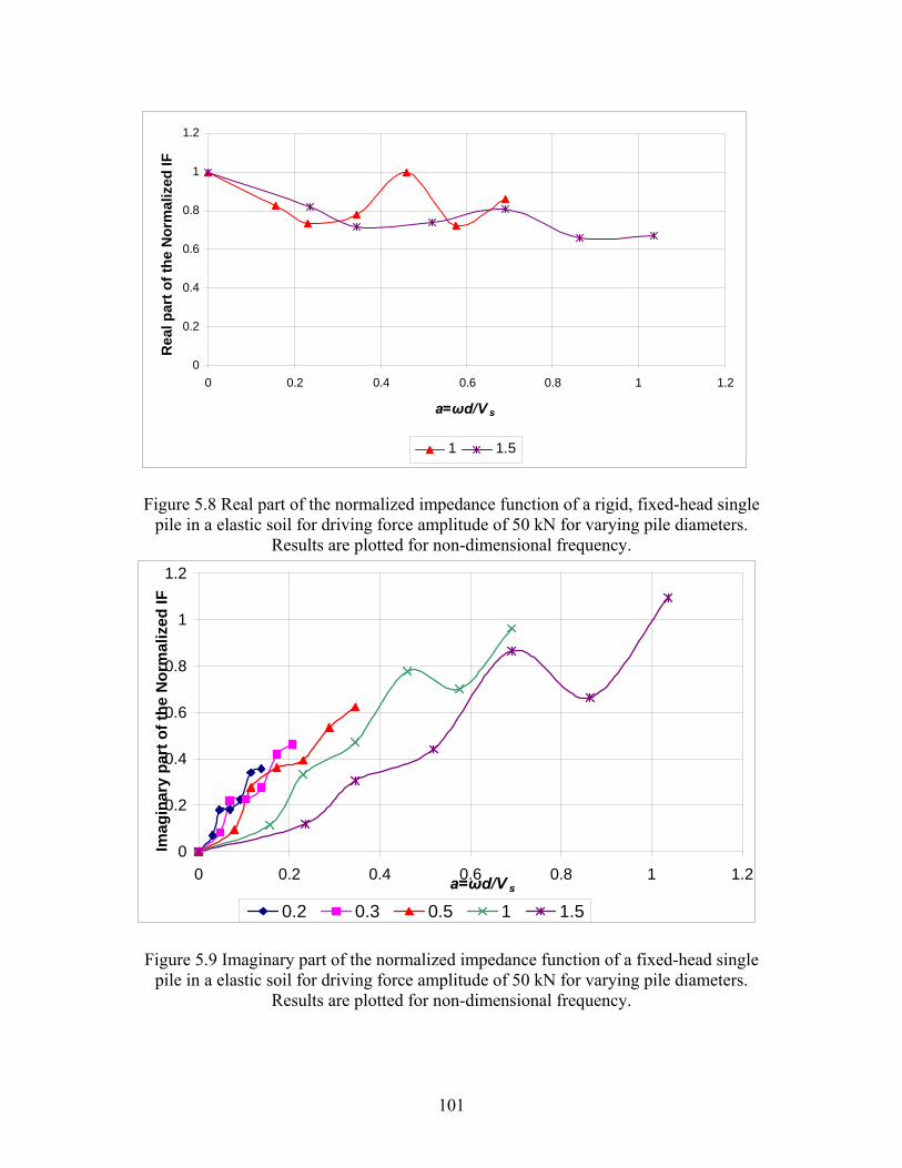
0

0.2

0.4

0.6

0.8

1

1.2

0 0.2 0.4 0.6 0.8 1 1.2

a=ωd/V s

Rea

l par

t of t

he N

orm

aliz

ed IF

1 1.5

Figure 5.8 Real part of the normalized impedance function of a rigid, fixed-head single pile in a elastic soil for driving force amplitude of 50 kN for varying pile diameters.

Results are plotted for non-dimensional frequency.

0

0.2

0.4

0.6

0.8

1

1.2

0 0.2 0.4 0.6 0.8 1 1.2a=ωd/V s

Imag

inar

y pa

rt o

f the

Nor

mal

ized

IF

0.2 0.3 0.5 1 1.5

Figure 5.9 Imaginary part of the normalized impedance function of a fixed-head single pile in a elastic soil for driving force amplitude of 50 kN for varying pile diameters.

Results are plotted for non-dimensional frequency.

101

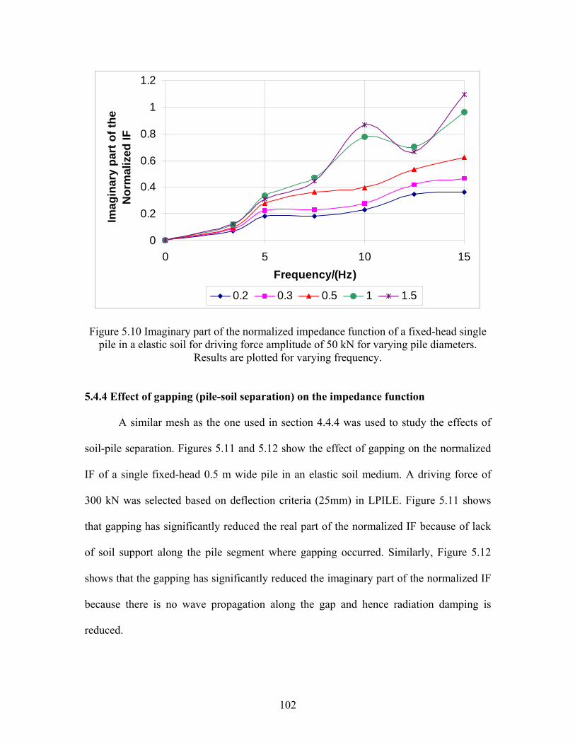
0

0.2

0.4

0.6

0.8

1

1.2

0 5 10Frequency/(Hz)

Imag

inar

y pa

rt o

f the

N

orm

aliz

ed IF

15

0.2 0.3 0.5 1 1.5

Figure 5.10 Imaginary part of the normalized impedance function of a fixed-head single

pile in a elastic soil for driving force amplitude of 50 kN for varying pile diameters. Results are plotted for varying frequency.

5.4.4 Effect of gapping (pile-soil separation) on the impedance function

A similar mesh as the one used in section 4.4.4 was used to study the effects of

soil-pile separation. Figures 5.11 and 5.12 show the effect of gapping on the normalized

IF of a single fixed-head 0.5 m wide pile in an elastic soil medium. A driving force of

300 kN was selected based on deflection criteria (25mm) in LPILE. Figure 5.11 shows

that gapping has significantly reduced the real part of the normalized IF because of lack

of soil support along the pile segment where gapping occurred. Similarly, Figure 5.12

shows that the gapping has significantly reduced the imaginary part of the normalized IF

because there is no wave propagation along the gap and hence radiation damping is

reduced.

102

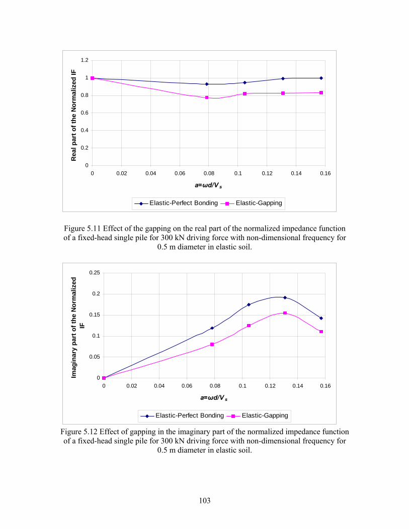
0

0.2

0.4

0.6

0.8

1

1.2

0 0.02 0.04 0.06 0.08 0.1 0.12 0.14 0.16

a=ωd/V s

Rea

l par

t of t

he N

orm

aliz

ed IF

Elastic-Perfect Bonding Elastic-Gapping

Figure 5.11 Effect of the gapping on the real part of the normalized impedance function of a fixed-head single pile for 300 kN driving force with non-dimensional frequency for

0.5 m diameter in elastic soil.

0

0.05

0.1

0.15

0.2

0.25

0 0.02 0.04 0.06 0.08 0.1 0.12 0.14 0.16

a=ωd/V s

Imag

inar

y pa

rt o

f the

Nor

mal

ized

IF

Elastic-Perfect Bonding Elastic-Gapping

Figure 5.12 Effect of gapping in the imaginary part of the normalized impedance function of a fixed-head single pile for 300 kN driving force with non-dimensional frequency for

0.5 m diameter in elastic soil.

103

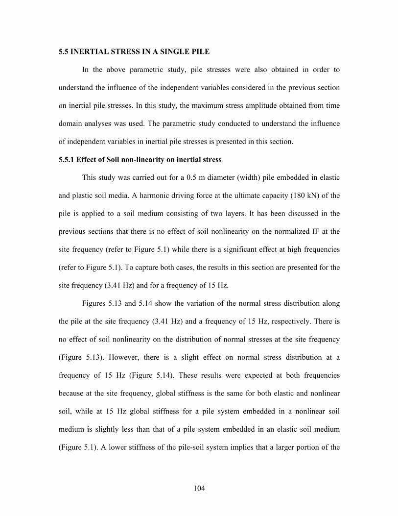
5.5 INERTIAL STRESS IN A SINGLE PILE

In the above parametric study, pile stresses were also obtained in order to

understand the influence of the independent variables considered in the previous section

on inertial pile stresses. In this study, the maximum stress amplitude obtained from time

domain analyses was used. The parametric study conducted to understand the influence

of independent variables in inertial pile stresses is presented in this section.

5.5.1 Effect of Soil non-linearity on inertial stress

This study was carried out for a 0.5 m diameter (width) pile embedded in elastic

and plastic soil media. A harmonic driving force at the ultimate capacity (180 kN) of the

pile is applied to a soil medium consisting of two layers. It has been discussed in the

previous sections that there is no effect of soil nonlinearity on the normalized IF at the

site frequency (refer to Figure 5.1) while there is a significant effect at high frequencies

(refer to Figure 5.1). To capture both cases, the results in this section are presented for the

site frequency (3.41 Hz) and for a frequency of 15 Hz.

Figures 5.13 and 5.14 show the variation of the normal stress distribution along

the pile at the site frequency (3.41 Hz) and a frequency of 15 Hz, respectively. There is

no effect of soil nonlinearity on the distribution of normal stresses at the site frequency

(Figure 5.13). However, there is a slight effect on normal stress distribution at a

frequency of 15 Hz (Figure 5.14). These results were expected at both frequencies

because at the site frequency, global stiffness is the same for both elastic and nonlinear

soil, while at 15 Hz global stiffness for a pile system embedded in a nonlinear soil

medium is slightly less than that of a pile system embedded in an elastic soil medium

(Figure 5.1). A lower stiffness of the pile-soil system implies that a larger portion of the

104

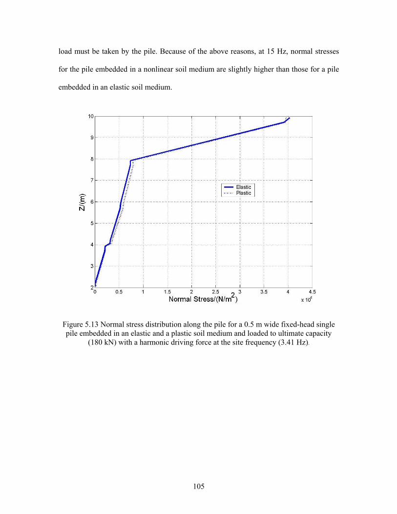
load must be taken by the pile. Because of the above reasons, at 15 Hz, normal stresses

for the pile embedded in a nonlinear soil medium are slightly higher than those for a pile

embedded in an elastic soil medium.

Figure 5.13 Normal stress distribution along the pile for a 0.5 m wide fixed-head single pile embedded in an elastic and a plastic soil medium and loaded to ultimate capacity

(180 kN) with a harmonic driving force at the site frequency (3.41 Hz).

105

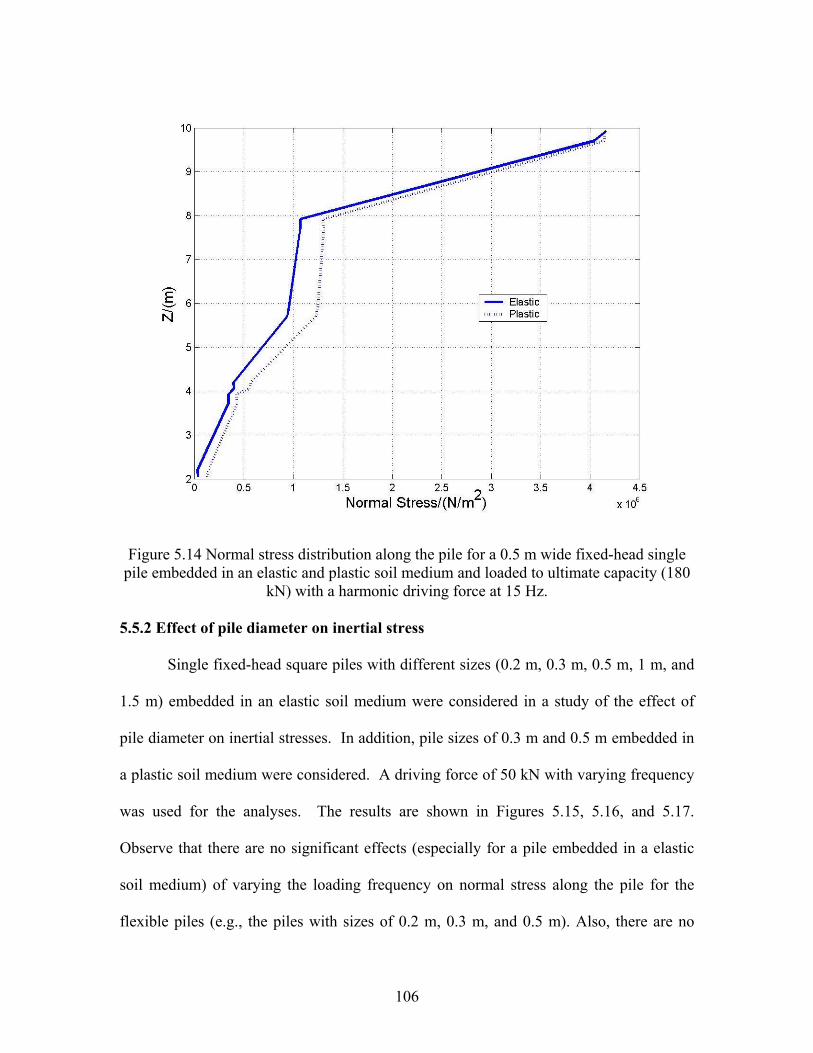
Figure 5.14 Normal stress distribution along the pile for a 0.5 m wide fixed-head single pile embedded in an elastic and plastic soil medium and loaded to ultimate capacity (180

kN) with a harmonic driving force at 15 Hz. 5.5.2 Effect of pile diameter on inertial stress

Single fixed-head square piles with different sizes (0.2 m, 0.3 m, 0.5 m, 1 m, and

1.5 m) embedded in an elastic soil medium were considered in a study of the effect of

pile diameter on inertial stresses. In addition, pile sizes of 0.3 m and 0.5 m embedded in

a plastic soil medium were considered. A driving force of 50 kN with varying frequency

was used for the analyses. The results are shown in Figures 5.15, 5.16, and 5.17.

Observe that there are no significant effects (especially for a pile embedded in a elastic

soil medium) of varying the loading frequency on normal stress along the pile for the

flexible piles (e.g., the piles with sizes of 0.2 m, 0.3 m, and 0.5 m). Also, there are no

106

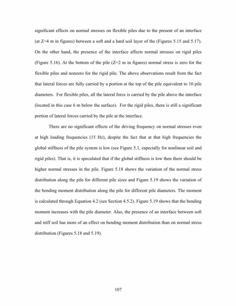
significant effects on normal stresses on flexible piles due to the present of an interface

(at Z=4 m in figures) between a soft and a hard soil layer of the (Figures 5.15 and 5.17).

On the other hand, the presence of the interface affects normal stresses on rigid piles

(Figure 5.16). At the bottom of the pile (Z=2 m in figures) normal stress is zero for the

flexible piles and nonzero for the rigid pile. The above observations result from the fact

that lateral forces are fully carried by a portion at the top of the pile equivalent to 10 pile

diameters. For flexible piles, all the lateral force is carried by the pile above the interface

(located in this case 6 m below the surface). For the rigid piles, there is still a significant

portion of lateral forces carried by the pile at the interface.

There are no significant effects of the driving frequency on normal stresses even

at high loading frequencies (15 Hz), despite the fact that at that high frequencies the

global stiffness of the pile system is low (see Figure 5.1, especially for nonlinear soil and

rigid piles). That is, it is speculated that if the global stiffness is low then there should be

higher normal stresses in the pile. Figure 5.18 shows the variation of the normal stress

distribution along the pile for different pile sizes and Figure 5.19 shows the variation of

the bending moment distribution along the pile for different pile diameters. The moment

is calculated through Equation 4.2 (see Section 4.5.2). Figure 5.19 shows that the bending

moment increases with the pile diameter. Also, the presence of an interface between soft

and stiff soil has more of an effect on bending moment distribution than on normal stress

distribution (Figures 5.18 and 5.19).

107

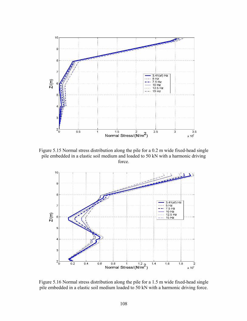
Figure 5.15 Normal stress distribution along the pile for a 0.2 m wide fixed-head single pile embedded in a elastic soil medium and loaded to 50 kN with a harmonic driving

force.

Figure 5.16 Normal stress distribution along the pile for a 1.5 m wide fixed-head single pile embedded in a elastic soil medium loaded to 50 kN with a harmonic driving force.

108

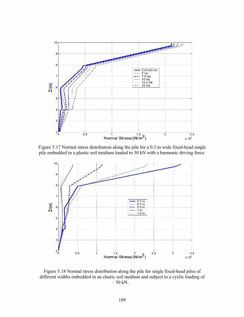
Figure 5.17 Normal stress distribution along the pile for a 0.3 m wide fixed-head single pile embedded in a plastic soil medium loaded to 50 kN with a harmonic driving force.

Figure 5.18 Normal stress distribution along the pile for single fixed-head piles of different widths embedded in an elastic soil medium and subject to a cyclic loading of

50 kN.

109

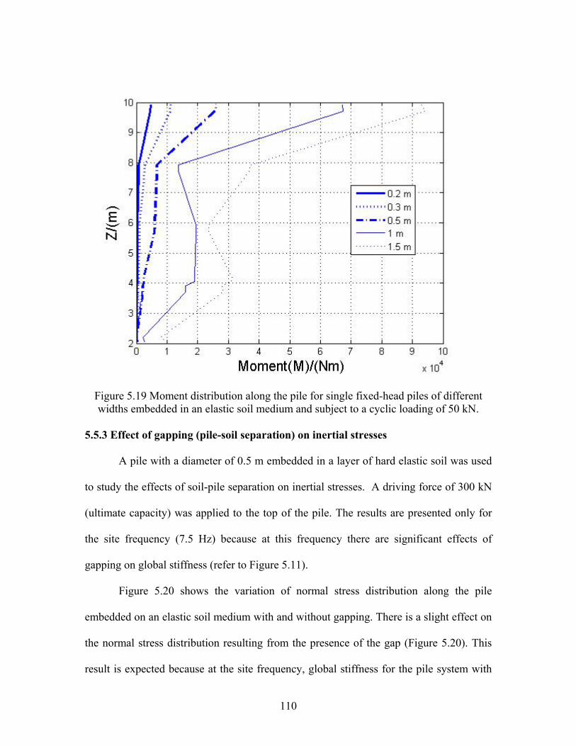
Figure 5.19 Moment distribution along the pile for single fixed-head piles of different widths embedded in an elastic soil medium and subject to a cyclic loading of 50 kN.

5.5.3 Effect of gapping (pile-soil separation) on inertial stresses

A pile with a diameter of 0.5 m embedded in a layer of hard elastic soil was used

to study the effects of soil-pile separation on inertial stresses. A driving force of 300 kN

(ultimate capacity) was applied to the top of the pile. The results are presented only for

the site frequency (7.5 Hz) because at this frequency there are significant effects of

gapping on global stiffness (refer to Figure 5.11).

Figure 5.20 shows the variation of normal stress distribution along the pile

embedded on an elastic soil medium with and without gapping. There is a slight effect on

the normal stress distribution resulting from the presence of the gap (Figure 5.20). This

result is expected because at the site frequency, global stiffness for the pile system with

110

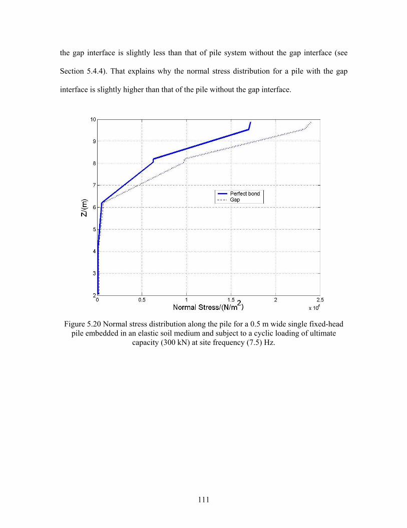
the gap interface is slightly less than that of pile system without the gap interface (see

Section 5.4.4). That explains why the normal stress distribution for a pile with the gap

interface is slightly higher than that of the pile without the gap interface.

Figure 5.20 Normal stress distribution along the pile for a 0.5 m wide single fixed-head

pile embedded in an elastic soil medium and subject to a cyclic loading of ultimate capacity (300 kN) at site frequency (7.5) Hz.

111

CHAPTER 6

CONCLUSIONS AND RECOMMENDATIONS

6.1 SUMMARY

Numerical models for dynamic soil-pile-structure interaction (SPSI) were developed

using the finite element software ABAQUS. The numerical models were developed for

quantifying kinematic transfer functions and inertial impedance functions for the design

of foundations subject to machine vibrations or ground shaking. This project also

involved developing a user subroutine for contact interaction and implementing a

constitutive model with stiffness proportional damping in a user subroutine umat. This

study was carried out for a single fixed-head pile. Tapered harmonic bedrock input

motions were used to quantify the kinematic transfer functions and a harmonic loading

function applied as a lateral force at the top of the pile was used to quantify the inertial

impedance functions. The multiaxial cyclic plasticity model of Borja and Amies (1994),

implemented in a FE code by Rodriguez-Marek (2000) was used in this study to model

soil nonlinearity and hysteretic behavior. Three independent variables were considered in

parametric studies. These variables are soil nonlinearity, pile diameter, and soil-pile

separation. A soft clay over a stiff clay soil profile was considered in the study of the

effects of pile diameter and soil nonlinearity on both kinematic transfer functions and

inertial impedance functions. For the study of soil-pile separation, a single layer of a hard

soil was used. A study also was conducted to evaluate the variation of normal stress along

the pile length as the independent variables were varied.

The treatment of the lateral boundary conditions presented in this study is a novel

approach that can lead to the use of smaller finite element meshes and hence aid future

112

researchers in this area. While this type of boundaries was previously implemented in

finite difference analyses, this is the first such implementation in FE. In addition,

researchers and practitioners alike will benefit from the parametric study presented in this

thesis, as it identifies the conditions under which soil nonlinearity, soil-pile separation,

and pile diameter effects become important in the treatment of kinematic and inertial

effects. The FE method proved to be a useful tool to study the effect of various variables

on the kinematic transfer functions as well as inertial impedance functions. This chapter

presents the major findings from this study and presents recommendations for further

study.

6.2 CONCLUSION

Conclusions from this study are categorized into two groups: those dealing with

kinematic interaction and those dealing with inertial interaction. For both cases, the

influence of various parameters on the TF as well as on the IF is described. These

parameters include soil nonlinearity, pile diameter, soil-pile separation, and intensity of

the harmonic input motion or loading function.

6.2.1 Kinematic interaction

I. Ground motion intensity does not change the value of the TF in a nonlinear soil

medium. While an increase in input motion intensity decreases the soil stiffness

and increases the hysteretic damping in the soil, these effects occur both for the

free field motion and the pile-top motion; hence the TF is not affected (Table 4.3

and Figure 4.4).

II. Transfer functions for a flexible pile embedded in an elastic soil medium have a

unique trend when plotted versus non-dimensional frequency a, where the

113

frequency is rendered non-dimensional by a =ωd/Vs. However, this uniqueness is

not preserved when the pile is embedded in a nonlinear soil medium. The

influence of the pile diameter (width) on the TF for a given frequency is

significant. However, the influence is not significant, especially for piles

embedded in an elastic soil medium, if the frequency axis is normalized as

discussed above (Figures 4.5 and 4.7).

III. The response of flexible piles embedded in an elastic soil medium is roughly

equal to free field response for frequencies up to 15 Hz (e.g., the value of the TF

is close to one). However, the response of flexible piles embedded in a nonlinear

soil differs from free field response, especially at high frequencies. Nonlinearity

of the soil medium reduces the transfer function significantly. This has more

effect on the 0.3 m wide pile. That is, an increase in the non-dimensional

frequency for the 0.3m wide pile increases the difference between the TF’s of

elastic and plastic soil models (Figures 4.3, 4.6, and 4.8).

IV. Separation between soil and pile has no effect in the transfer function of a pile

embedded in an elastic soil medium (Table 4.4).

V. Maximum normal stresses on a pile occur when the harmonic excitation

frequency is equal to the linear site frequency (where fsite = Vs/(4H)). The

maximum normal stress on flexible piles occurs at the depth of the interface

between soft and hard soils. On the other hand, the maximum normal stress on

rigid piles occurs at the pile top. For flexible piles, the maximum normal stress is

nearly independent of pile diameter and the normal stress on the pile top increases

114

with pile width. For rigid piles normal stresses along the entire pile length are

smaller for piles with smaller width (Figures 4.12, 4.13, 4.14, and 4.17).

The maximum bending moment envelope along the pile increases with

pile width for both rigid and flexible piles, but the shape of the envelope is a

function of pile width. The normalization of bending moment proposed by

Kavvadas and Gazetas (1993) renders a pile-top bending moment that is

independent of diameter (except for 1.5 m diameter), however the normalization

does not result in a unique bending moment envelope along the pile (Figures 4.15

and 4.16).

VI. Generally, nonlinearity does not affect significantly the normal stress envelope

along the pile. However, at the site frequency, nonlinearity reduced the normal

stress at the top of the pile by 35 %. For higher frequencies (e.g. 15 Hz), soil

nonlinearity does not have a systematic effect on the normal stress envelope (e.g.,

stresses increase at some depths and decrease at others) (Figures 4.10 and 4.11).

VII. Soil-pile separation (gapping) increases the normal stress along the lower half of a

flexible pile. However, there is no effect of gapping on the normal stresses in the

upper half portion of the pile (Figure 4.18).

6.2.2 Inertial interaction

I. The magnitude of the driving force does not affect the IF of a pile embedded in an

elastic soil medium. However, the IF of a pile embedded in a nonlinear soil

medium is affected by the magnitude of the driving force. That is, the real part of

the IF reduces with increasing driving force magnitude. On the other hand, the

115

imaginary part of the IF increases with increasing driving force magnitude

(Figures 5.3, 5.4, 5.5, and 5.6).

II. For flexible piles embedded in an elastic soil medium, the real part of the IF is

nearly constant across all frequencies and does not change much with pile

diameter. For rigid piles, the real part of the IF reduces with increasing frequency.

For flexible pile the imaginary part of the IF has unique trend in non-dimensional

frequency but for rigid pile the imaginary part of the IF decreases with increasing

diameter for a given non-dimensional frequency (Figures 5.7, 5.8, 5.9, and 5.10).

III. Soil nonlinearity reduces slightly the real part of the IF for low loading

frequencies and significantly for high loading frequencies. On the other hand, soil

nonlinearity increases the imaginary part of the IF (Figures 5.1 and 5.2).

IV. Soil-pile separation (gapping) reduces the real and imaginary parts of the IF

(Figures 5.11 and 5.12).

V. The normal stress envelope along a pile embedded in elastic soil medium is not

affected by loading frequency, in particular for flexible piles. However, there is a

considerable effect of loading frequency on the normal stress envelope when the

pile is embedded in a nonlinear soil. Furthermore, the presence of an interface

between soft and hard soil has been found to affect the maximum normal stresses

for rigid piles, but not for flexible piles. At the bottom of the pile, normal stresses

are zero for flexible piles and nonzero for rigid piles. The bending moment

envelope increases with increasing pile width (Figures 5.15, 5.16, and 5.17).

VI. Nonlinearity does not affect the normal stress along the pile at low frequencies

and it has a small effect at higher frequencies (Figures 5.13 and 5.14).

116

VII. Soil-pile separation increases the normal stress along the pile (Figure 5.20).

6.3 RECOMMENDATION FOR FUTURE RESEARCH

Recommendations for further research on the subject of kinematic transfer

functions and inertial impedance functions are listed below.

I. The effect of soil-pile separation on the TF as well as the IF has to be studied for

the plastic soil model. In this study, gapping was only considered for an elastic

soil.

II. Analysis for the TF and the IF should be carried out for pile groups with different

spacing and inclinations.

III. The study of soil-pile separation on the TF as well as the IF should be extended to

pile groups. The effects of pile spacing and pile inclination should be studied.

IV. A study should be carried out to validate the superposition assumption made in

this study, in particular for nonlinear soils.

117

REFERENCES

ABAQUS. (2005). Hibbitt, karlsson and Sorensen., Inc., Version 6.5.

Ahmad, S. and Mamoon, S.M. (March 11-15,1991). “Seismic Response of Floating Piles to Obliquely Incident Waves.” Proc. of 2nd International Conference on Recent Advances in Geotechnical Earthquake Engineering and Soil Dynamics, St. Louis, MO., University of Missouri-Rolla Publication, pp.805-814.

American petroleum Institute (API) (1987). “Recommended practice for planning, designing, and constructing fixed offshore platforms.” API Recommended Practice 2A (RP-2A), 17th edn.

Anandarajah, A. and Zhang, J. (2000). “Simplified finite element modeling of nonlinear dynamic pile-soil interaction.” Retrieved February 10, 2005, from http://www.ce.utexas.edu/em2000/papers/AAnand_2.pdf.

ANSYS Inc. (1996). “General finite element analysis program.” Version 5.4. ANSYS, Inc., Canonsburg, Pa.

Bardet, J.P. (1989). “Prediction of deformations of Hostun and Reid Bedford sands with a simple bounding plasticity model.” in Constitutive Equations for Granular Non-cohesive Soils, A. Saada and G. Bianchini, Eds., pp.131-148, Balkema.

Bentley, K.J. Naggar, M.H.EI. (2000). “Numerical analysis of kinematic response of single piles.” Canadian Geotechnical Journal, 37, pp. 1368-1382.

Borja, R.I. and Amies, A.P. (1994). “Mutiaxial Cyclic Plasticity Model for Clays,” Journal of Geotechnical Engineering, ASCE, 120(6), pp. 1051-1070.

Borja, R.I., Chao, H.Y., Montans, F.J., and Lin, C.H. (1999). “Nonlinear ground response at Lotung LSST site.” Journal of Geotechnical and Geoenvironmental Engineering, ASCE, 125, pp. 187-197.

Borja, R.I., Lin, C-H., Sama, K. M., and Masada, G. M. (2000). “Modeling non-linear ground response of non-liquefiable soils.” Earthquake Engineering and Structural Dynamics, 29, pp. 63-83.

Borja, R.I., Duvernay, B.G., and Lin, C-H. (2002). “Ground Response in Lotung: Total Stress Analyses and parametric Studies.” Journal of Geotechnical and Geoenvironmental Engineering, 128(1), pp. 54-63

Boulanger, R.W., Wilson, D.W., Kutter, B.L., and Abghari, A. (1999). “Soil-pile-superstructure interaction in liquefiable sand.” Transportation research record 1569, pp. 55-64.

118

Bransby, M. F. (1999). “Selection of p-y curves for the design of single laterally loaded piles.” International Journal for Numerical and Analytical Methods in Geomechanics, 23(15), pp. 1909-1926.

Brown, D.A., O’Neill, M.W., Hoit, M., Mcvay, M., Naggar, M.H.EI., and Chakraborty, S. (2001). “Static and dynamic lateral loading of pile groups.” NCHRP report, 461, Appendix B

Butterfield, R. and Banerjee, P. K. (1971). “The Elastic Analysis of Compressible Piles and Pile Groups.” Geotechnique, 21, pp. 43-60.

Cai, Y.X., Gould, P.L., and Desai, C.S. (2000). “Nonlinear analysis of 3D seismic interaction of soil-pile-structure system and application.” Engineering Structures, 22, pp. 191-199.

Cox, W. R., Reese, L. C., and Grubbs, B. R. (1974). “Field testing of laterally loaded piles in sand.” Proc. 6th Offshore Technology conference, Paper 2079, Houston, Texas, pp. 459-472.

Dafalias, Y.F. and Popov, E.P. (1975). “A model of non-linearity hardening material for cyclic loading.” Acta mechanical, 21, pp. 173-192.

Dafalias, Y.F. and Popov, E.P. (1977). “Cyclic loading for materials with a vanishing elastic region.” Nuclear Engineering and Design, 41, North-Holland, Amsterdam, The Netherlands, pp. 293-302.

Dafalias, Y.F. (1986). “Bounding surface plasticity, I: Mathematical foundation and hypoplasticity.” Journal of Engineering Mechanics, ASCE, 112, pp. 966-987

Desai, C. S., Drumm, E. C. and Zaman, M. M. (1985). “Cyclic Testing and Modeling of Interfaces.” Journal of Geotechnical Engineering, ASCE, 111 (6), pp.793-815.

Desai, C. S. and Nagaraj, B. K. (1986). “Constitutive Modeling in Nonlinear Soil-Structure Interaction.” In Mechanics of Material Interfaces, A. P. S. Selvadurai and G. Z. Voyiadjis, eds., Elsevier Science Publishers, Amsterdam.

Desai, C. S., Zaman, M. M., Lightner J. G. and Siriwardane, H. J. (1984). “Thin-Layer Element for Interfaces and Joints.” International Journal for Numerical and Analytical Methods in Geomechanics, 8 (1), pp. 19-43.

Dobry, R. and Gazetas, G. (1988). “ Simple method for dynamic stiffness and damping of floating pile groups.” Geotechnique, 38, pp. 557-574.

Drumm, E. C. (1983). “Testing, modeling, and application of interface behavior in dynamic soil-structure interaction.” Dissertation presented to the University of

119

Arizona, at Tucson, Arizona, in partial fulfillment of the requirements for the degree of Doctor of Philosophy.

Drumm, E. C. and Desai, C.S. (1986). “Determination of Parameters for a Model for Cyclic Behavior of Interfaces.” Journal of Earthquake Engineering and Structural Dynamics, 16 (1), pp. 1-18.

Duncan, J. M. and Chang, C-Y. (1970). “Nonlinear analysis of stress and strain in soil.” JSMFE, ASCE, 96 (SM5), pp. 1629-1653

Dunnavant, T. W. (1986). “Experimental and analytical investigation of the behavior of single piles in overconsolidated clay subjected to cyclic lateral loads.” Ph.D. Dissertation, University of Houston, Houston, Texas.

Dunnavant, T. W. and O’Neill, M. W. (1985). “Performance analysis and interpretation of a lateral load test of a 72-inch-diameter bored pile in overconsolidated clay.” Report UHCE 85-4, Department of Civil Engineering, University of Houston, Texas, p. 57.

Eurocode 8-part 5. (1999) “Foundations, retaining structures and geotechnical aspects.” Ref. No prEN 1998-5.

Fan, K., Gazetas, G., Kaynia, A., Kausel, E., and Ahmad, S. (1991). “Kinematic Seismic Response of Single Piles and Pile Groups.” Journal of Geotechnical Engineering, Proc. ASCE, 117 (12), pp. 1860-1879.

Finn, W. D. L. (1988). “Dynamic analysis in geotechnical engineering.” Proceedings, Earthquake Engineering and Soil Dynamics II – Recent Advances in Ground Motion Evaluations. Geotechnical Special Publication, 20, ASCE, pp. 523-591.

Finn, L.W.D., Wu, G., and Thavaraj, T. (1997). “Soil-pile-structure interactions.” Geotechnical Special Publication, 70, pp. 1-22.

FLAC 3D, (2002). Fast lagrangian analysis of continua in 3 dimensions, Itasca consulting group,inc., Minnesota, Version 2.1.

Gazetas, G. and Dobry, R. (1984). “Horizontal Response of Piles in Layered Soils.” Journal of Geotechnical Engineering, Proc. ASCE, 110 (1), pp. 20-40.

Gazetas, G. (1984). “Seismic response of end bearing piles.” Soil Dynamic and Earthquake Engineering, 3 (2), pp. 82-93.

Gazetas, G. and Mylonakis, G. (1998). “Seismic soil structure interaction: new evidence and emerging issues.” Geotechnical Earthquake Engineering and Soil Dynamics, ASCE, II, pp. 1119-1174.

120

Ghaboussi, J., Wilson, E. L., and Isenberg, J. (1973). “Finite element for rock joint and interfaces.” Journal of Soil Mechanics and Foundation Engineering Division, ASCE, 99 (10), pp. 833-848.

Gohl, W.B. (1991). “Response of pile foundations to simulated earthquake loading: Experimental and analytical results.” Ph.D. thesis, Department of Civil Engineering, The University of British Columbia, Vancouver.

Goodman, R. E., Taylor, R. L., and Brekke, T. L. (1968) “A model for the mechanics of jointed rock.” Journal of Soil Mechanics and Foundation Engineering Division, ASCE, 94 (3), pp. 637-660.

Hardin, B. O. and Drnevich, V. P. (1972). “Shear modulus and damping in soils: measurements and parameter effects.” Journal of Soil Mechanics and Foundation Engineering Division, ASCE, 98(SM6), pp. 603-624.

Herrmann, L. R. (1978). “Finite element analysis of contact problems.” Journal of Soil Mechanics Division, ASCE, 104 (5).

Hudson, M., Idriss, I. M., and Beikae, M. (1994). “QUAD4M: A Computer Program to Evaluate the Seismic Response of Soil Structures using Finite Element Procedures and Incorporating a Compliant Base.” Center for Geotechnical Modeling, Department Of Civil and Environmental Engineering, University of California, Davis.

Idriss, I. M. et al. (1979). “Analysis of soil-structure interaction effects for nuclear power plants.” Report by the Ad Hoc Group on Soil-Structure Interaction. ASCE, New York, N.Y.

International Code Council, ICC (2003). International Building Code, International Code Council, Country Club Hills, IL.

Isenberg, J. and Vaughan,D. K. (1981). ”Nonlinear effect in Soil-Structure Interaction.” Proc. of the symposium on implementation of Comp. Procedures and Stress-Strain Laws in Geotechnical Engineering, held at Chicago, III.

Ismael, N. F. (1990) “Behavior of laterally loaded bored piles in cemented sands.” Journal of Geotechnical Engineering, ASCE, 116(11), pp. 1678-1699.

Juirnarongrit, T. (2002). “Effect of Diameter on the Behavior of laterally Loaded Piles in Weakly Cemented Sand.” Ph.D. thesis, Department of civil engineering, University of California, San Diego.

Katona, M. G. (1981). “A simple contact-friction interface element with applications to buried culverts.” Proc., Implementation of Computer Proc. and Stress-Strain Laws in Geotechnical Engineering, held at Chicago, III.

121

Kavvadas, M. and Gazetas, G. (1993). “Kinematic seismic response and bending of free-head piles in layered soil.” Geotechnique, 43 (2), pp. 207-222.

Kausel, E. and Peek, R. (1982). “Boundary integral method for Stratified Soils.” Res. Re, R82-50, MIT, Cambridge, MA.

Kausel, E. and Roesset, J.M. (1974). “Soil- Structure interaction for Nuclear Containment Structures.” Proc. ASCE, Power Division Specialty Conference, Boulder, Colorado.

Kaynia, A. M. and Kausel, E. (1982). “Dynamic Behavior of Pile Groups.” Proc. 2nd int. Conference, On Numerical Methods in Offshore Piling, Texas University, Austin, pp. 509-532.

Kim, S. and Stewart, J. P. (2003). “Kinematic Soil-Structure Interaction from Strong Motion Recordings.” Journal of Geotechnical and Environmental Engineering, ASCE, 129 (4), pp. 323-335.

Kishishita, T., Saito, E., and Miura, F. (2000). “Dynamic-response characteristics of structures with micropile foundation system.” 12th World Conference on Earthquake Engineering, Auckland, New Zealand, pp. 1-8.

Kramer, S. L. (1996). Geotechnical Earthquake Engineering, Prentice Hall, Engelwood Cliffs N.J.

Lanzo, G. and Vucetic, M. (1999). “Effect of soil plasticity on damping ratio at small cyclic strains.” Soils and Foundations, 39(4), pp. 131-141.

Lysmer, J. and Kuhlemeyer, R.L. (1969). “Finite dynamic model for infinite media.” Journal of the Engineering Mechanics Division, ASCE, 95(EM 4), pp. 859-877.

Maheshwari, B.K., Truman, K.Z., Naggar, M.H.EI., and Gould, P.L. (2004). “Three dimensional finite element nonlinear dynamic analysis of pile groups for lateral transient and seismic excitations.” Canadian Geotechnical Journal, 41, pp. 118-133.

Makris, N. and Gazetas, G. (1992). “Dynamic pile-soil-pile interaction.” Part II: Lateral and seismic response.” Earthquake Engineering and Structural Dynamics, 21, pp. 145-162.

Mamoon, S. M. and Ahmad, S. (1990). “Seismic response of piles to obliquely incident SH, SV, and P waves.” Journal Geotechnical Engineering, 116 (2), pp. 186-204.

Matlock,H. (1970). “Correlation for design of laterally loaded piles in soft clay.” Proc.,2nd Annu. Offshore Technology Conference, Paper No. OTC 1204,Houston, Texas, pp. 577-594.

122

Nogami, T. and Konagai, K. (1986). “Time domain axial response of dynamically loaded single piles.” Journal of Engineering Mechanics, ASCE, 112(11), pp. 1241-1252.

Nogami, T. and Konagai, K. (1988). “Time domain flexural response of dynamically loaded single piles.” Journal of Engineering Mechanics, ASCE, 114(9), pp. 1512-1525.

Nogami, T., Otani, J., Konagai, K., and Chen, H. L. (1992).”Nonlinear soil-pile interaction model for dynamic lateral motion.” Journal of Geotechnical Engineering, ASCE, 118(1), pp. 89-106.

Naggar, M. H. EI. and Novak, M. (1995). “Nonlinear lateral interaction in pile dynamics.” Journal of Soil Dynamics and Earthquake Engineering, 14, pp. 141-157.

Naggar, M. H. EI. and Novak, M. (1996). “Nonlinear Analysis for Dynamic Lateral Pile Response.” Journal of Soil Dynamics and Earthquake Engineering, 15 (4), pp. 233-244.

Novak, M. and Mitwally, H. (1988). “Transmitting boundary for axisymmetrical dilation problems.” Journal of Engineering Mechanics, ASCE, 114 (1), pp. 181-187

O’Neill, M. W. and Dunnavant, T. W. (1984). “A study of effect of scale, velocity, and cyclic degradability on laterally loaded single piles in overconsolidated clay.” Report UHCE 84-7, Department of Civil Engineering, University of Houston, Texas, p. 368.

O’Neill, M. W. and Murchison, J. M. (1983). “An evaluation of p-y relationships in sands.” A report to the American Petroleum Institute.” PRAC 82-41-1, University of Houston, Texas.

Ousta, R. and Shahrour, I. (2001). “Three-dimensional analysis of the seismic behavior of micropiles used in the reinforcement of saturated soil.” International Journal for Numerical and Analytical Methods in Geomechanics, 25, pp. 183-196.

Penzien, J. (1970). “Soil-Pile Foundation Interaction.” Earthquake Engineering, Chapter 14, Prentice-Hall, pp. 349-381.

Poulos, H. G. (1968). “Analysis of the Settlement of Pile Groups.” Geotechnique, 18 (4), pp. 449-471.

Poulos, H. G. (1971). “Behaviour of Laterally-Loaded Piles, II: Pile Groups.” Journal of Soil Mechanics and Foundation Engineering, ASCE, 97(SM5), pp. 773-751.

Prager, W. (1956).”A new method of analyzing stresses and strains in work-hardening plastic solids.” Journal of Applied Mechanics, (Dec), pp. 493-496.

123

Prevost, J. H. (1977). “Mathematical modeling of monotonic and cyclic undrained clay behavior.” International Journal of Numerical Analysis Methods in Geomechanics, 1, pp.195-216.

Reese, L. C., Cox, W. R., and Koop, F. D. (1974). “Analysis of laterally loaded piles in sand.” Proc. 6th Offshore Technology Conference, Paper 2080, Houston, Texas, pp. 473-483.

Reese, L. C., Cox, W. R., and Koop, F. D. (1975). “Field testing and analysis of laterally loaded piles in stiff clay.” Proc. 7th Offshore Technology Conference, Paper No. OTC 2321, Houston, Texas, pp. 671-690.

Reese, L. C., Wang, S. T., Isenhower, W. M., and Arrellaga, J.A. (2000). Computer Program LPILE Plus Version 4.0 Technical Manual, Ensoft, Inc., Austin, Texas.

Reese, L. C. and Welch, R. C. (1975). “Lateral loading of deep foundation in stiff clay.” Journal of Geotechnical Engineering Division, ASCE, 101(7), pp. 633-649.

Rodriguez-Marek, A. (2000). “Near-fault seismic site response.” Ph.D. Dissertation, University of California, Berkeley.

Rodriguez-Marek, A. and Bray, J. D. “Seismic Site Response for Near-Fault Ground Motions.” Journal of Geotechnical and Geoenvironmenatl Engineering, submitted on June 2005.

Roesset, J. M. and Scarletti, H. (1979). “Nonlinear effects in dynamic soil-structure interaction.” Proc., 3rd International Conference on Numerical Methods in Geomechanics, Balkema Press. Rotterdam. The Netherlands.

Sadek, M. and Shahrour, I. (2003). “Influence of piles inclination on the seismic behavior of groups of flexible piles.” 82nd Annual Meeting of the Transportation Research Board, pp. 1-14.

Sen, R., Davies, T. G., and Banerjee, P. K. (1985). “Dynamic Analysis of piles and Pile Groups Embedded in Homogeneous Soils.” Earthquake Engineering and Structural Dynamics, 13, pp. 53-65.

Shahrour, I., Sadek, M., and Ousta, R. (2001). “Seismic behavior of micropiles used as foundation support elements.” Transportation Research Record 1772, pp. 84-90.

Simo, J.C. and Hughes, P.J.R. (1998). Computational Inelasticity. Interdisciplinary Applied Mathematics. IAM (Springer).

Stevens, J. B. and Audibert, J. M. E. (1979). “Re-examination of p-y curve formulation.” Proc. Of the XI Annual Offshore Technology Conference, Houston, Texas, OTC 3402, pp. 397-403.

124

Toki, K., Sato, T., and Miura, I. (1981). “Separation and Sliding between soil and

structure during strong ground motion.” Earthquake Engineering and Structural Dynamics, 9 (3), pp. 263-277.

Zaman, M. M., Desai, C. S. and Drumm, E. C. (1984). “An Interface Model for Dynamic Soil-Structure Interaction.” Journal of Geotechnical Engineering Division, ASCE, 110 (9), pp.1257-1273.

Zhao, C. and Valliappan, S. (1993). “A dynamic infinite element for three dimensional infinite-domain wave problem.” International Journal for Numerical Methods in Engineering, 36:2567-80

Zienkiewicz, C., Chang, C.T., and Bettess, P. (1980). “Drained, undrained, consolidating and dynamic behavior assumptions in soils.” Geotechnique, 30, pp. 385-395.

Zienkiewicz, O. C., Emson, C., and Bettess, P. (1983). “Novel boundary infinite element.” International Journal for Numerical Methods in Engineering, 19 (3), pp. 393-404.

Zienkiewicz, O.C. and Shiomi, T. (1984). “Dynamic behavior of saturated porous media: The generalized biot formulation and its numerical solution.” International Journal for Numerical and Analytical Methods in Geomechanics, 8:71-96.

University of Florida (1996). User’s Manual for FLORIDA-PIER Program, Department of Civil Engineering, University of Florida, Gainesville.

Vaughan, D.K. and Isenberg, J. (1983). “Nonlinear rocking response of model containment structures.” Earthquake Engineering and Structural Dynamics, 11.

Wang, S. and Reese, L. C. (1993). “COM624P-Laterally loaded pile analysis program for the microcomputer, version 2.0.” FHWA-SA-91-048, U.S. DOT, Federal Highway Administration.

Welch, R. C. and Reese, L. C. (1972). “Laterally loaded behavior of drilled shafts.” Research Report 3-5-65-89, Center for Highway Research, University of Texas, Austin.

Whitman, R.V. (1972). “Analysis of Soil-Structure Interaction: State-of -the-Art Review.” Experimental and Structural Dynamics, Inst. Of Sound and Vibration, Southampton.

Wilson, D.W. (1998). “Soil-pile superstructure interaction in liquefiable sand and soft clay.” Doctoral dissertation, University of California, Davis, pp. 173

125

Wolf, J. P. (1985). “Dynamic soil-structure interaction.” Prentice-Hall. Inc., Englewood Cliffs, N. J.

Wu, G. (1994). “Dynamic soil-structure interaction: Pile foundations and retaining structures.” Ph.D. Dissertation, University of British Columbia.

Wu, G. and Finn, D.L.W. (1997). “Dynamic elastic analysis of pile foundations using finite element method in the frequency domain.” Canadian Geotechnical Journal, 34(1), pp. 34-43.

Wu, G. and Finn, D.L.W. (1997). “Dynamic nonlinear analysis of pile foundations using finite element method in the time domain.” Canadian Geotechnical Journal, 34(1), pp. 44-52.

126