Embed Size (px)
Citation preview

1
Computational Electronics Group
2002 School on Computational Material Science May 21-31, 2002
Numerical methods for the solution ofSchrödinger equation for ballistic
transport
Umberto Ravaioli
Beckman Institute andDepartment of Electrical and Computer Engineering
University of Illinois at Urbana-ChampaignUrbana, IL 61801, USA
University of Illinois

2 2002 School on Computational Material Science May 21-31, 2002
Time-dependent Schrödinger Equation• Goal of quantum mechanics is to give a quantitative
description on a microscopic scale of individual elementaryobjects (electrons, photons, atoms,…) which behave both likeparticles and waves, exhibiting diffraction and interferencephenomena.
• Propagation cannot be described by a trajectory r ( t ) as for aclassical particle, but by a field-like quantity ψ (r,t ) calledwave function. The simplest wave function is a plane wave
with mechanical and wave parameters related as
( ) ( )0 ˆ, exp = ⋅ − r t j k r tψ Ψ ω
( ) ( ); ; ;= = = =dispersion relations
p k E k E E pω ω ω
3 2002 School on Computational Material Science May 21-31, 2002
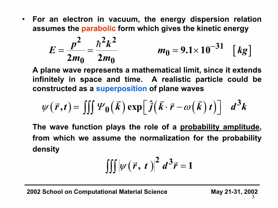
• For an electron in vacuum, the energy dispersion relationassumes the parabolic form which gives the kinetic energy
A plane wave represents a mathematical limit, since it extendsinfinitely in space and time. A realistic particle could beconstructed as a superposition of plane waves
The wave function plays the role of a probability amplitude,from which we assume the normalization for the probabilitydensity
[ ]2 2 2
310
0 09.1 10
2 2−= = = ×
p kE m kgm m
( ) ( ) ( )( ) 30 ˆ, exp = ⋅ − ∫∫∫r t k j k r k t d kψ Ψ ω
( ) 2 3, 1=∫∫∫ r t d rψ

4 2002 School on Computational Material Science May 21-31, 2002
• The evolution of the wave function is described by theSchrödinger equation
which is actually a system of two equations for the real andimaginary part of the wave function
( ) ( ) ( )2
2
0
,ˆ , ( ) ,2
∂= − ∇ +
∂r t
j r t V r r tt m
ψψ ψ
( ) ( )( ) ( ) ( ) ( )
( ) ( ) ( ) ( )
22
02
2
0
ˆ
2
2
= ℜ + ℑ
∂ ℜ= − ∇ ℑ + ℑ
∂
∂ ℑ= − ∇ ℜ + ℜ
∂
j
V rt m
V rt m
ψ ψ ψ
ψψ ψ
ψψ ψ

5 2002 School on Computational Material Science May 21-31, 2002
• In operator notation the solution to Schrödinger equation is
with the system Hamiltonian
This represents a formal solution of the Schrödinger equationas a first order differential equation in time. Except for trivialcases, we cannot find an analytical form for the exponentialterm containing the Hamiltonian.
All numerical solutions must find a suitable approximation ofthe exponential on a set of discrete points.
( ) ( )ˆ
, exp ,0
= −
jr t H t rψ ψ
( )2
2
02= − ∇ +H V r
m

6 2002 School on Computational Material Science May 21-31, 2002
• Consider a discretization of the domain involving N meshpoints
The discretized form of the solution is
. . . . . . . .
1 2 3 N-1 N
( ) ( )
( ) matrix representing the discretized Hamiltonian
solution array defined on the mesh points
ˆexp 0
∗ =
=
+ = −
jt t H t
Ht
ψ ∆ ∆
ψ
ψ

7 2002 School on Computational Material Science May 21-31, 2002
• We need to find a numerical approximation for theexponential of the discretized operator
satisfying:
a) stability of the iteration
b) conservation of the wave function probability
c) consistency ( we really solve the intended equation )
ˆexp
−
j H t∆

8 2002 School on Computational Material Science May 21-31, 2002
1-D time-dependent Schrödinger equation
Let’s illustrate the properties of numerical solutions byusing finite-differences on a uniform mesh.
A discretization may require
Explicit numerical methods – if it only requires a directsubstitution of values in the formulation
Implicit methods – if it involves solution of a linear systemof equations
( ) ( ) ( )22
20
, ,ˆ ( ) ,2
x t x tj V r x t
t m xψ ψ
ψ∂ ∂
= − +∂ ∂

9 2002 School on Computational Material Science May 21-31, 2002
A. Simple (naïve) explicit method
A simple direct finite difference discretization gives
In operator notation
UNSTABLE and NON-CONSERVING
( ) ( ) ( ) ( ) ( ) ( )
( ) ( ) ( ) ( ) ( ) ( )
2
20
20
; 1 ; 1; 2 ; 1;ˆ ( ) ;2
1; 2 ; 1; ( )ˆ; 1 ; ;2
i n i n i n i n i nj V i i n
t m x
i n i n i n V ii n i n j t i nm x
y y y y y yD D
y y yy y D yD
+ - - - + += - +
Ê ˆ- - + ++ = + +Á ˜
Ë ¯
( ) ( )ˆ
1
+ = −
jn I H t nψ ∆ ψ

10
B. Three-time-levels explicit method
A centered time difference is applied
To obtain the operator algorithm, we need to eliminate theintermediate solution at iteration n
STABLE and UNITARY (CONSERVING)
2002 School on Computational Material Science May 21-31, 2002
( ) ( ) ( ) ( ) ( ) ( )20
1; 2 ; 1; ( )ˆ; 1 ; 1 2 ;2
i n i n i n V ii n i n j t i nm x
y y yy y D yD
Ê ˆ- - + ++ = - + +Á ˜
Ë ¯
( ) ( )( ) ( )
ˆ1 1ˆ
I jH tn n
I jH t
∆ψ ψ
∆
−⇒ + ≈ −
+
( ) ( ) ( )1 12
+ − −=
n nn
ψ ψψ

11
C. Fully implicit method
Discretize space operator at timestep ( j+1) leading to a system thatrequires a matrix inversion
In operator notation
STABLE but NON-UNITARY (NON-CONSERVING)
2002 School on Computational Material Science May 21-31, 2002
( ) ( ) ( ) ( ) ( )
( )20
1; 1 2 ; 1 1; 1 ( )ˆ; 1 ; 12
; 1
i n i n i n V ii n j t i nm x
i n
y y yy D yD
y
Ê ˆ- + - + + + ++ + + +Á ˜
Ë ¯
= -
( ) ( )1ˆ
1−
+ = +
jn I H t nψ ∆ ψ
12
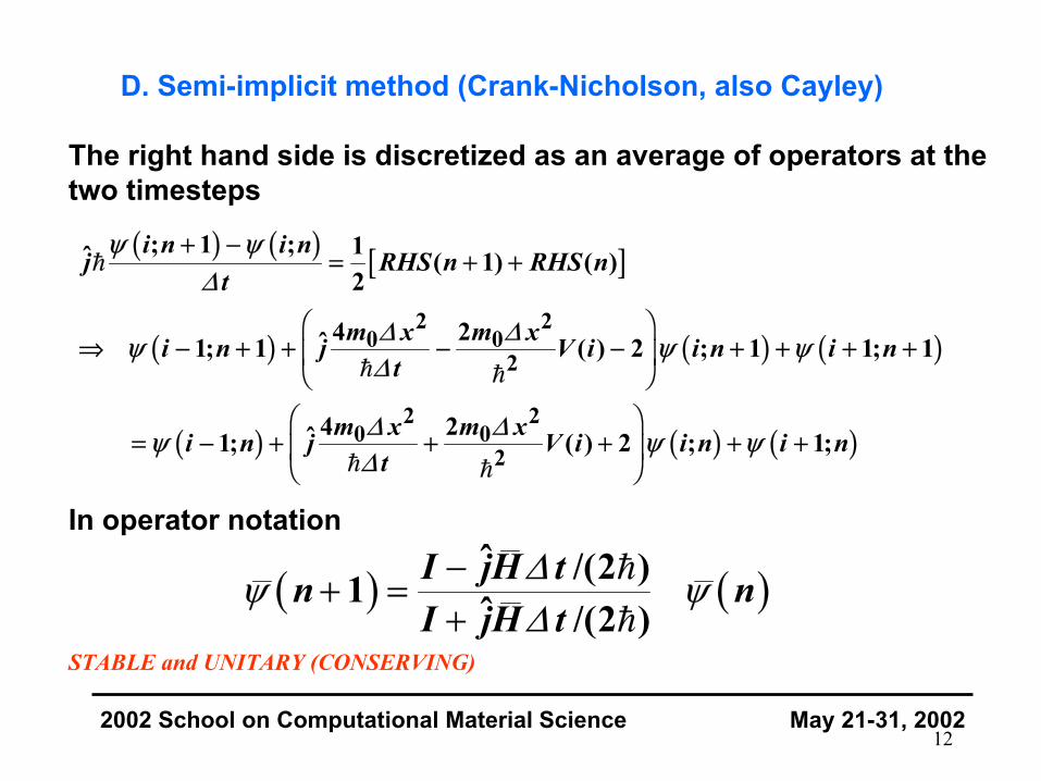
D. Semi-implicit method (Crank-Nicholson, also Cayley)
The right hand side is discretized as an average of operators at thetwo timesteps
In operator notation
STABLE and UNITARY (CONSERVING)
2002 School on Computational Material Science May 21-31, 2002
( ) ( ) [ ]
( ) ( ) ( )
( ) ( ) ( )
2 20 0
2
2 20 0
2
; 1 ; 1ˆ ( 1) ( )2
4 2ˆ1; 1 ( ) 2 ; 1 1; 1
4 2ˆ1; ( ) 2 ; 1;
i n i nj RHS n RHS n
t
m x m xi n j V i i n i nt
m x m xi n j V i i n i nt
y yD
D Dy y yD
D Dy y yD
+ -= + +
Ê ˆfi - + + - - + + + +Á ˜
Ë ¯
Ê ˆ= - + + + + +Á ˜
Ë ¯
( ) ( )ˆ /(2 )1 ˆ /(2 )
−+ =
+I jH tn nI jH t
∆ψ ψ∆

13
Of the schemes analyzed, only the three time steps explicit
and the Crank Nicholson semi-implicit method
are suitable.
One can see that the numerical operators are essentiallyequivalent.
2002 School on Computational Material Science May 21-31, 2002
( ) ( )ˆ /(2 )1 ˆ /(2 )
−+ =
+I jH tn nI jH t
∆ψ ψ∆
( ) ( )( ) ( )
ˆ /1 1ˆ /
I jH tn n
I jH t
∆ψ ψ
∆
−+ ≈ −
+
14
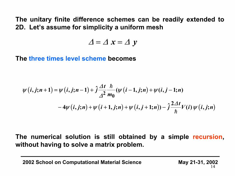
The unitary finite difference schemes can be readily extended to2D. Let’s assume for simplicity a uniform mesh
The three times level scheme becomes
The numerical solution is still obtained by a simple recursion,without having to solve a matrix problem.
2002 School on Computational Material Science May 21-31, 2002
= =x y∆ ∆ ∆
( ) ( ) ( )
( ) ( ) ( ) ( )
2 0ˆ, ; 1 , ; 1 ( 1, ; ( , 1; )
2ˆ4 , ; 1, ; , 1; ) ( ) , ;
ti j n i j n j i j n i j nm
ti j n i j n i j n j V i i j n
Dy y y yD
Dy y y y
+ = - + - + -
- + + + + -
15
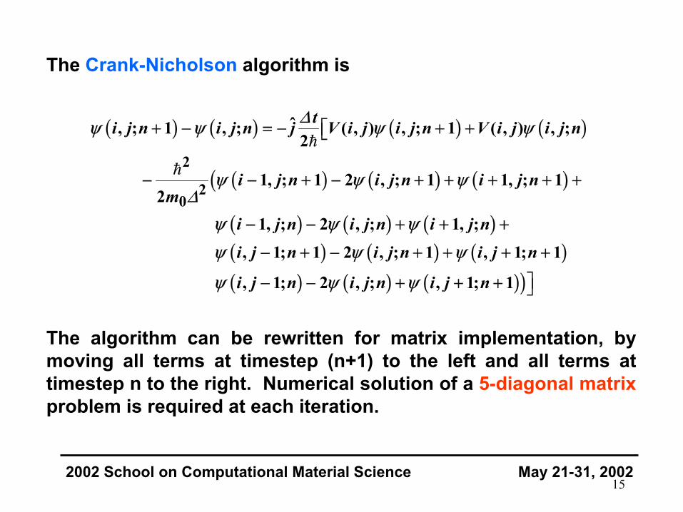
The Crank-Nicholson algorithm is
The algorithm can be rewritten for matrix implementation, bymoving all terms at timestep (n+1) to the left and all terms attimestep n to the right. Numerical solution of a 5-diagonal matrixproblem is required at each iteration.
2002 School on Computational Material Science May 21-31, 2002
( ) ( ) ( ) ( )
( ) ( ) ( )(
( ) ( ) ( )( ) ( ) ( )( ) ( ) ( ))
2
20
ˆ, ; 1 , ; ( , ) , ; 1 ( , ) , ;2
1, ; 1 2 , ; 1 1, ; 12
1, ; 2 , ; 1, ;
, 1; 1 2 , ; 1 , 1; 1
, 1; 2 , ; , 1; 1
ti j n i j n j V i j i j n V i j i j n
i j n i j n i j nm
i j n i j n i j n
i j n i j n i j n
i j n i j n i j n
Dy y y y
y y yD
y y yy y y
y y y
+ - = - + +ÈÎ
- - + - + + + + +
- - + + +
- + - + + + +
˘- - + + + ˚

16
To alleviate the requirements of the matrix solution, it is possibleto use an Alternate Direction Implicit (ADI) scheme. The timestep is split into two sub-steps of half duration, and twoconsecutive sets of solutions are performed:
Horizontal sweep
2002 School on Computational Material Science May 21-31, 2002
( ) ( )( ( )
( )( ) ( )
( ) ( )( ( )
( )( ) ( )
2
20
2
20
ˆ, ; 1/ 2 1, ; 1/ 2 2 , ; 1/ 22 2
( , )1, ; 1/ 2 , ; 1/ 22
ˆ, ; , 1; 2 , ;2 2
( , ), 1; , ;2
ti j n j i j n i j nm
V i ji j n i j n
ti j n j i j n i j nm
V i ji j n i j n
Dy y yD
y y
Dy y yD
y y
È+ + - - + - +Í
Í΢+ + + + + =˙̊
È- - - -Í
Í΢+ + + ˙̊

17
Vertical sweep
2002 School on Computational Material Science May 21-31, 2002
( ) ( )( ( )
( )( ) ( )
( ) ( )( ( )
( )( ) ( )
2
20
2
20
ˆ, ; 1 , 1; 1 2 , ; 12 2
( , ), 1; 1 , ; 12
ˆ, ; 1/ 2 1, ; 1/ 2 2 , ; 1/ 22 2
( , )1, ; 1/ 2 , ; 1/ 22
ti j n j i j n i j nm
V i ji j n i j n
ti j n j i j n i j nm
V i ji j n i j n
Dy y yD
y y
Dy y yD
y y
È+ + - - + - +Í
Í΢+ + + + + =˙̊
È+ - - - + - +Í
Í΢+ + + + + ˙̊

18
The ADI procedure decouples adjacent rows and columns ofmesh points. For every sweep, a set of tridiagonal systems issolved.
Because of the decoupling, the tridiagonal solutions in eachsweep can be carried out independently, therefore the approachis suitable for supercomputing applications (vectorization,parallelization).
In the numerical scheme shown here, the contribution by thepotential is equally divided between the implicit part (left handside) and the explicit part (right hand side) of the algorithm.
Note: the intermediate solution after a horizontal sweep is stillvery biased. Only solutions obtained after two consecutivesweeps should be considered.
2002 School on Computational Material Science May 21-31, 2002

19
Possible discussion items:
How can one implement a self-consistent solution (Poissonequation solved at each iteration to update the potential) in athree-time-step explicit method or in a semi-implicit method,where the potential should be known for the “next” timestepalready?
What trade-offs and approximations are possible/reasonable?
2002 School on Computational Material Science May 21-31, 2002
20
Systems with variable effective mass
In the effective mass approximation, the potential V in theSchrödinger equation is assumed to be only the electrostaticpotential, since the effect of the periodic crystal is accounted forby the effective mass itself.
However, some of the most interesting applications of quantumsystems involve spatially varying materials and heterojunctions.The effective mass approximation can still be used with somecaution.
When the effective mass is space-dependent, the major issue isto find the Hamiltonian operator, so that it remains Hermitian.
2002 School on Computational Material Science May 21-31, 2002

21
If we just insert a space dependent mass in the Schrödinger as iswe know that the Hamiltonian is not Hermitian. Also, this methodwould be mathematically applicable only to slowly varying mass.A widely used Hermitian form brings the effective inside theLaplacian differential operator
This operator can be used also for transport across abruptheterojunctions, as long as the materials on the two sides havesimilar properties and band structure (e.g. AlGaAs/GaAs).
But one has to keep in mind that very close to the heterojunctionthe physical properties, described by the effective massSchrödinger equation, are not necessarily well defined.
2002 School on Computational Material Science May 21-31, 2002
2
*1
2 − ∇ ⋅ ∇ m
ψ
22
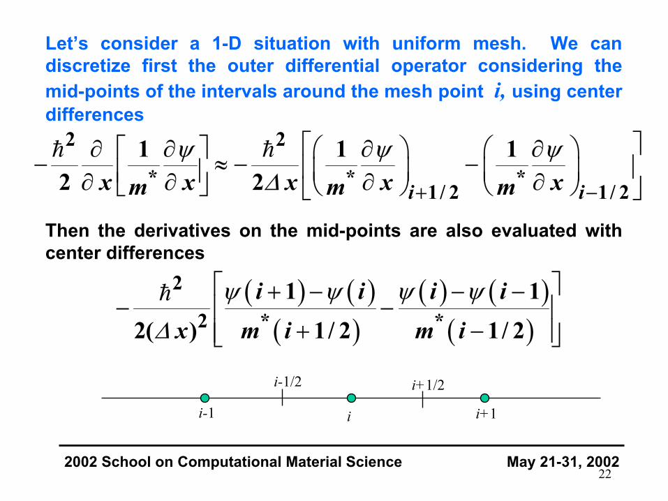
Let’s consider a 1-D situation with uniform mesh. We candiscretize first the outer differential operator considering themid-points of the intervals around the mesh point i, using centerdifferences
Then the derivatives on the mid-points are also evaluated withcenter differences
2002 School on Computational Material Science May 21-31, 2002
2 2
* * *1/ 2 1/ 2
1 1 12 2 + −
∂ ∂ ∂ ∂ − ≈ − − ∂ ∂ ∂ ∂ i ix x x x xm m mψ ψ ψ
∆
( ) ( )( )
( ) ( )( )
2
2 * *1 1
2( ) 1/ 2 1/ 2
+ − − −− −
+ −
i i i ix m i m i
ψ ψ ψ ψ
∆
i-1 i+1i
i+1/2i-1/2
23
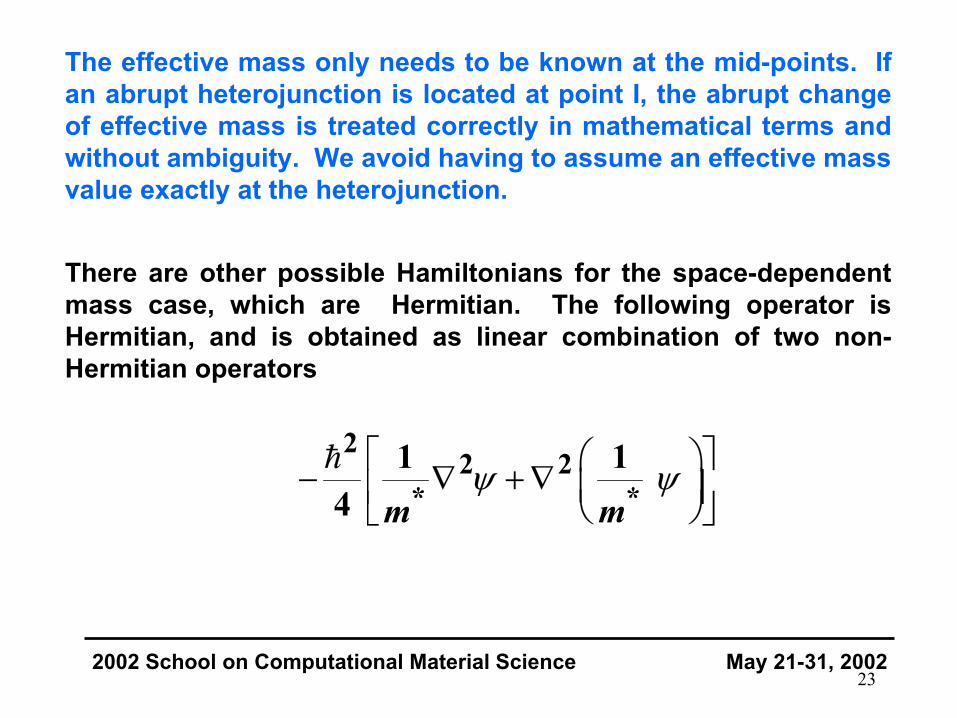
The effective mass only needs to be known at the mid-points. Ifan abrupt heterojunction is located at point I, the abrupt changeof effective mass is treated correctly in mathematical terms andwithout ambiguity. We avoid having to assume an effective massvalue exactly at the heterojunction.
There are other possible Hamiltonians for the space-dependentmass case, which are Hermitian. The following operator isHermitian, and is obtained as linear combination of two non-Hermitian operators
2002 School on Computational Material Science May 21-31, 2002
22 2
* *1 1
4 − ∇ + ∇ m m
ψ ψ

24
Let’s compare the two Hamiltonians, in a 1-D formulation
2002 School on Computational Material Science May 21-31, 2002
2 2 2
* * 2 *
2 2 2
* 2 2 *
2 2
* 2 *
extra term
2
2 *
1 1 12 2
1 1 4
1 1 2
1 00
12
∂ ∂ ∂ ∂ ∂ − = − + ∂ ∂ ∂ ∂ ∂ ∂ ∂ − + =
∂ ∂ ∂ ∂ ∂ − + ∂ ∂ ∂
∂ + ∂
x x x xm m x m
m x x m
x xm x m
x m
ψ ψ ψ
ψ ψ
ψ ψ
ψ

25
For smoothly varying mass, the two approaches areapproximately equivalent. One can see that it is awkward todirectly discretize with finite differences the numerical operatorson the right hand side. The proper procedure is to use boxintegration, over the interval [ i-1/2; i+1/2 ]. Integration by partscan be applied
2002 School on Computational Material Science May 21-31, 2002
1 1 2
1 1 2
1 1 2
1 2
1 1 2
1 2
2 2
* 2 *
2
* *
1 12
1 12
+
−
+
−
+
−
∂ ∂ ∂ − + = ∂ ∂ ∂
∂ ∂ ∂ − − ∂ ∂ ∂
∫
∫
i
i
d xx x xm x m
d xx x x xm m
ψ ψ∆
ψ ψ∆
1 1 2
1 2 *1+
−
∂ ∂ + ∂ ∂ ∫i
d xx x m
ψ
same as previous result

26
Absorbing boundary conditionsNumerical solution of the time-dependent Schrödinger equationis often accomplished by assuming a gaussian wave packetdistribution describing the particle. The boundaries of thesystems are taken to be far away from the simulated region, andthe wave function there is fixed to zero.
As the simulation progresses, the wave packet spreads andintercats with potential variations, originating reflectedwavepackets. Over a sufficient number of simulation steps, thewave may reach the boundaries, where the condition of zerowave function corresponds to perfect reflection!
2002 School on Computational Material Science May 21-31, 2002
ψ= 0ψ= 0
27
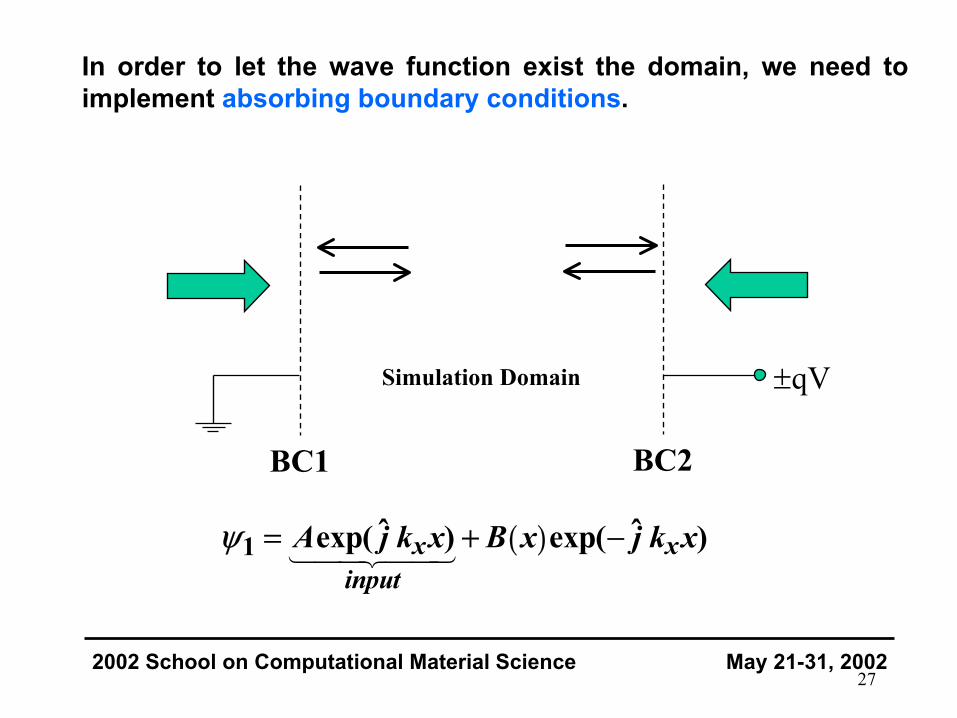
In order to let the wave function exist the domain, we need toimplement absorbing boundary conditions.
2002 School on Computational Material Science May 21-31, 2002
BC1 BC2
±qVSimulation Domain
( )1 ˆ ˆexp( ) exp( )x xinput
A j k x B x j k xy = + -

28
Assume B(x) approximately linear near the boundary BC1
2002 School on Computational Material Science May 21-31, 2002
( ) ( ) ( )22
20
0, 0,ˆ (0) 0,2
t tj V t
t m xψ ψ
ψ∂ ∂
= − +∂ ∂
( )
( ) ( )
2 2 ˆ ˆ20
2 2 2 ˆ
0 0
2
ˆ,2
x x
x
j k x j k xx
xj k xx x
A e B em x
Bk kx t j em m x
ψ
−=
−= +
∂− +∂
∂+∂
…

29
The formal solution of the differential equation in time gives
At BC2 similar treatment with
2002 School on Computational Material Science May 21-31, 2002
( ) ( ) ( )
( )
ˆ
ˆ
0
x
j E t
jk xx
t t t eB xk e t
tm
∆ψ ∆ ψ
∆
−
−∗
= ≈ =
∂+
∂
[ ]2
2BC
m E qVk
* -=

30
Create a new discretized equation near the boundaries
In a Crank-Nicholson scheme
2002 School on Computational Material Science May 21-31, 2002
( ) ( ) ( )
( ) ( )max max
01
2
B x B x BBC
t xB x B x x
BCx
∆∆
∆∆
∂ −=
∂
− −=
( ) ( ) ( )12
t t tB x B x B xt x x
∆+ ∂ ∂ ∂ = + ∂ ∂ ∂
31
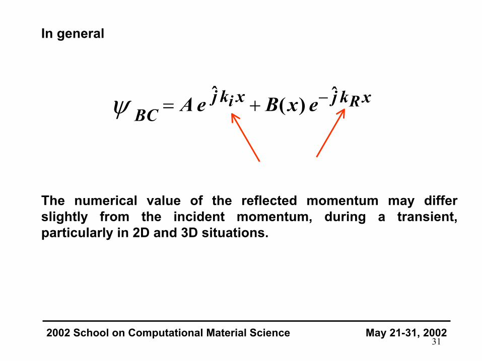
In general
The numerical value of the reflected momentum may differslightly from the incident momentum, during a transient,particularly in 2D and 3D situations.
2002 School on Computational Material Science May 21-31, 2002
ˆ ˆ( )i Rj k x j k xBC A e B x eψ −= +

32
Issue: discretization changes the relationship between(simulated) energy and momentum! Discetization creates avirtual lattice where transport is described by the Tight-BindingHamiltonian
2002 School on Computational Material Science May 21-31, 2002
r r x+ Dr x- DV̂
( )ˆ ˆ| 1 | | 1 || |ˆ rr
l V l l VH l ll E > < + > < -+<= +>Â
coupled pendula

33
Potential for transferring an electron from one site to a neighbor
Energy of an electron located at a lattice site
Atomic-like orbital centers at the sites (forming a regular lattice)
2002 School on Computational Material Science May 21-31, 2002
2
21ˆ hopping potential
2 ( )V
m x*= - =D
ˆ( ) 2rpotentialenergy
E V r V= -
| l >
r

34
In the continuum limit
For a periodic lattice
2002 School on Computational Material Science May 21-31, 2002
( )
( ) ( )0 0
( ) 01 ˆ| exp |
ˆexpl
ll
V r
k j k l x lN
E k E V j k l x
=
>= D >
= + D
Â
Â
2 2
2
finite difference approximation
ˆ ( )2
ˆ
dH H V rm d r
H
*Æ = - +
=
neighbors
35
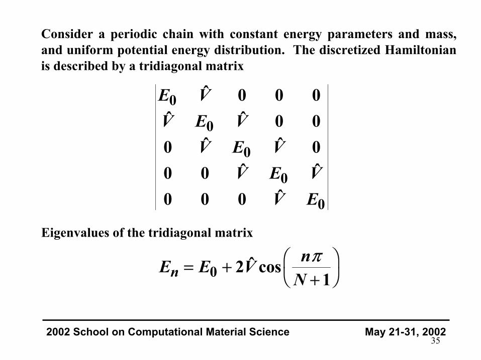
Consider a periodic chain with constant energy parameters and mass,and uniform potential energy distribution. The discretized Hamiltonianis described by a tridiagonal matrix
Eigenvalues of the tridiagonal matrix
2002 School on Computational Material Science May 21-31, 2002
0
0
0
0
0
ˆ 0 0 0ˆ ˆ 0 0
ˆ ˆ0 0ˆ ˆ0 0
ˆ0 0 0
E VV E V
V E VV E V
V E
0 ˆ2 cos1n
nE E VNpÊ ˆ= + Ë ¯+

36
Dispersion relationship for the discretized Hamiltonian is not parabolic!Absorbing boundary conditions for a discretized Hamiltonian should bederived in the tight-binding formalism.
2002 School on Computational Material Science May 21-31, 2002
( )0
0
0
ˆˆ( ) exp( )
ˆ ˆˆ exp( ) exp( )ˆ2 cos( )
lE k E V j k l
E V j k x j k x
E V k x
= +
= + D + - D
= + D
Â
xp- D xp D0
E
k

37 2002 School on Computational Material Science May 21-31, 2002
[ ]
( )
( )
0ˆ ˆ ˆ ˆ
0
ˆ0
0
ˆ ˆ
0ˆ ˆ0 0 1 1
ˆ0 (1) ( 1)
1 0
(1)
cons
(0)( )
ˆ ˆ0 0 (0
linear at boundary( 1) (0)
tant
)
ˆ(0)
jka jka jka jka
jka
jka j
H E V
E V Ae B e Ae B e
H E V e A B
e A
BC l x a
B B BB x
B B B
B
E
V B e
ψ
ψ ψ ψ ψ
∆
∆
ψ
ψ ψ
∆
∆
− −
− −
→ = =
= + −
= + + − =
= + + + + −
= +
=
+ +
+ + +
= −
( )ˆka jkae −
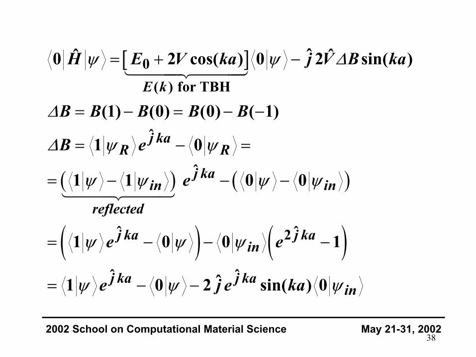
38 2002 School on Computational Material Science May 21-31, 2002
[ ]
( ) ( )
( ) ( )
0( ) for TBH
ˆ
ˆ
ˆ ˆ2
ˆ ˆ
ˆˆ ˆ0 2 cos( ) 0 2 sin( )
(1) (0) (0) ( 1)
1 0
1 1 0 0
1 0 0 1
ˆ1 0 2 sin( ) 0
E k
j kaR R
j kain in
reflected
j ka j kain
j ka j kain
H E V ka j V B ka
B B B B B
B e
e
e e
e j e ka
ψ ψ ∆
∆
∆ ψ ψ
ψ ψ ψ ψ
ψ ψ ψ
ψ ψ ψ
= + −
= − = − −
= − =
= − − −
= − − −
= − −

39
Final results for absorbing boundary conditions at input
has been eliminated
An even more refined methodology for absorbing boundary conditions can be found at: L.F. Register, U. Ravaioli and K. Hess, J. Applied Physics, vol. 69, pp. 7153-7158, 1991 (+ small corrections at the Erratum section of: J. Applied Physics, vol 71, p. 1555, 1992),
2002 School on Computational Material Science May 21-31, 2002
[ ]0ˆ
ˆ 2
ˆ0 2 cos( ) 0
ˆ ˆˆ ˆ2 sin( ) 0 2 sin( ) 1
ˆ4 sin ( ) 0
j ka
j kain
H E V ka
j V ka j V ka e
Ve ka
y y
y y
y
= +
+ -
-
Ry
40
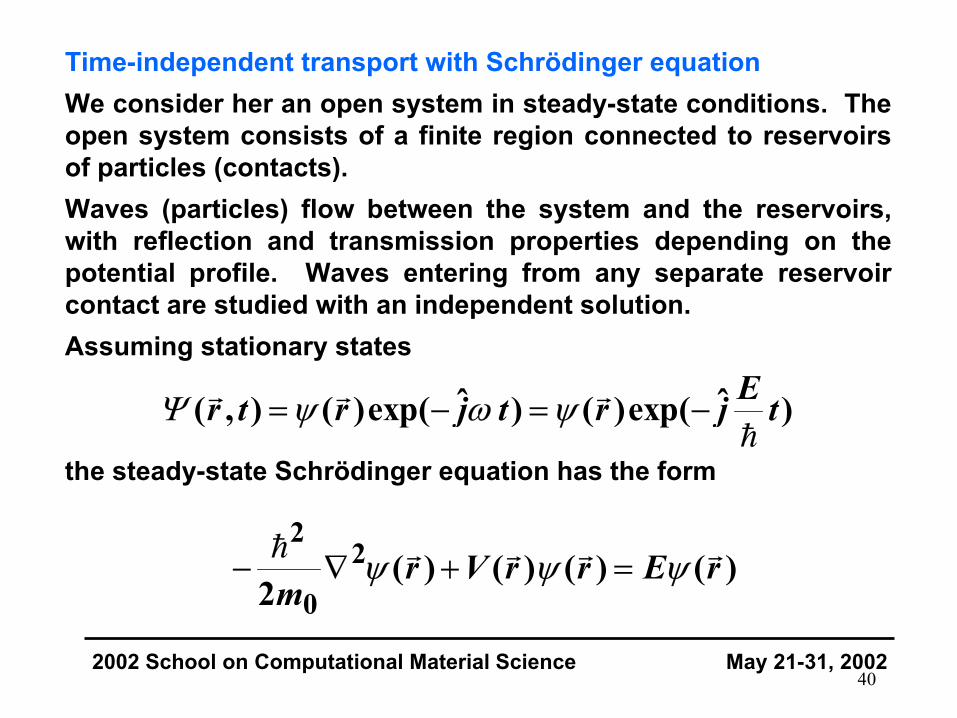
Time-independent transport with Schrödinger equationWe consider her an open system in steady-state conditions. Theopen system consists of a finite region connected to reservoirsof particles (contacts).Waves (particles) flow between the system and the reservoirs,with reflection and transmission properties depending on thepotential profile. Waves entering from any separate reservoircontact are studied with an independent solution.Assuming stationary states
the steady-state Schrödinger equation has the form
2002 School on Computational Material Science May 21-31, 2002
ˆ ˆ( , ) ( )exp( ) ( )exp( )Er t r j t r j tΨ ψ ω ψ= − = −
22
0( ) ( ) ( ) ( )
2r V r r E r
mψ ψ ψ− ∇ + =

41
Let’s consider a 1-D domain with uniform grid and mesh size ∆ x.The time independent Schrödinger equation is discretized withfinite differences
E represents the total energy, so that V(i) - E is the kineticenergy. It is often convenient to set the reference zero of thepotential V(x) at the inflow boundary, so that E corresponds tothe incident kinetic energy.
The kinetic energy varies spatially according to the potentialchanges, and the wavenumber kx(x) varies accordingly. Theknowledge of kx at the reservoir ends, allows the specification ofboundary conditions.
2002 School on Computational Material Science May 21-31, 2002
[ ]2
20
( 1) 2 ( ) ( 1) ( ) ( ) 02 ( )
i i i V i E im x
ψ ψ ψ ψ∆
− − + +− + − =

42
The travelling wave at the specified energy can be assumed to bea plane wave of the form
where the sign indicates the direction of propagation. Boundaryconditions are derived from this expression for both forward andbackward wave.
The exponentials are completely specified in the boundaryconditions by the knowledge of E and V(x). The prefactor A is setto a conventional reference (e.g., A=1) at the one boundary, andthe value at the other end is the outcome of the solution. Thesolution for the pre-factor A may be complex, and it contains theinformation on reflection and transmission coefficients.
2002 School on Computational Material Science May 21-31, 2002
( ) ( ) ( )ˆexp xx A x j k x xψ = ±
V = 0
E(x)
V (x)

43
In 1-D, all is needed for the solution is a recursion algorithm. Fora forward travelling wave which enters the open system at x = 0,we can set A( L ) = 1 ( L is the length of the domain) and obtainthe boundary condition
N is the index corresponding to the output boundary. Assumingthat the domain is subdivided into N mesh intervals, the index forthe left boundary is i = 0. To solve the open system problem, weneed to assume a perfect reservoir with a constant potential(ohmic contact) and no change in the wavevector kx
The knowledge of the wave function N and N+1 is sufficient tocalculate the value of ψ (N-1) using the discretized Schrödingerequation.
2002 School on Computational Material Science May 21-31, 2002
( ) ˆexp ( )xN j k N Lψ =
( ) ( )[ ]ˆ( ) ( 1) 1 exp ( )x x xk N k N N j k N L xψ ∆= + ⇒ + = +

44
The general recursion algorithm can be easily obtained byrewriting the discretized Schrödinger equation
The potential reference is V(0) = 0, so that E represents thekinetic energy
as well as the total energy at the inflow point i = 0.
2002 School on Computational Material Science May 21-31, 2002
( )2
01 12
2 ( )2 ( )i i im x V i E∆ψ ψ ψ− +
= + − −
2 2
0
(0)2
xkEm
=

45
Because of reflection due to the potential variations, throughoutthe device one can express the wave function as thesuperposition of an incident and a reflected wave
At the output, because of the constant potential in the reservoir,we assume that there is no reflection
At the input we can express the total wave function as
2002 School on Computational Material Science May 21-31, 2002
( ) ( ) ( )ˆ ˆexp ( ) exp ( )x xi I i j k i i x R i j k i i xψ ∆ ∆ = + −
( ) ( ) ( )0 and R N I N A N= =
( ) ( ) ( ) ( )0 0 0 0A I Rψ = = +

46
To find the amplitude of incident and reflected waves, we needan additional solution at a mesh point inside the input reservoir.With the same assumptions as for the output reservoir
By combining the above with
we obtain
Once I(0) is determined, the wave function throughout the devicecan be re-normalized to make the total probability unitary.
2002 School on Computational Material Science May 21-31, 2002
( ) ( ) ( )( ) ( ) ( )
; 1 1 1 1ˆ ˆ1 0 exp (0) 0 exp ( )x x
x x i I R
I j k x R j k i x
∆ ψ
ψ ∆ ∆
= − = − ⇒ − = − + −
− = − +
( ) ( ) ( ) ( )0 0 0 0A I Rψ = = +
( )( ) ( ) ( )
( )( )ˆ0 exp 0 1
0 ˆ2 sin 0x
x
j k xI
j k xψ ∆ ψ
∆
− − =

47
The procedure for inflow from the right boundary is essentiallythe same, with appropriate sign changes for the waves. Therecursion relation becomes
with the starting point
The recursions are solved for a set of energies and for inflowfrom both boundaries. In order to find the total result, one stillneeds to specify injection condition, that provide the weights foradding all the separate recursion results.
2002 School on Computational Material Science May 21-31, 2002
( )2
01 12
2 ( )2 ( )i i im x V i E∆ψ ψ ψ+ −
= + − −
( ) ( ) ˆ0 1 and 1 exp (0)xj k xψ ψ ∆ = − = −

48
We consider now a simple case for an n-type semiconductor,where the two reservoirs are assumed in quasi-equilibrium, witha specific Fermi level EF.
The equilibrium particle density, including the effect of spin, is
Assuming for simplicity an isotropic mass, the particle energy is
To determine the density for the injection direction, we need tointegrate over the transverse direction
2002 School on Computational Material Science May 21-31, 2002
( )[ ]31 1
1 exp /4x y z
F Bn dk dk dk
E E k Tπ∞−∞
=+ −∫∫ ∫
( )2 2 22 2
2 2
y zxx
k kkE E Em m
⊥ ∗ ∗
+= + = +

49
The integration is performed over the transverse momentumcomponents, in polar coordinates
The integration over the angle provides simply a factor 2π and achange of variable is performed
2002 School on Computational Material Science May 21-31, 2002
( )[ ]20 03
1 kk
1 exp /4x
x F Bn dk d d
E E E k Tπ
θπ
∞ ∞ ⊥⊥−∞
⊥=
+ + −∫ ∫ ∫
2k k
2k2
m EE
md dEE
∗⊥
⊥ ⊥ ⊥
∗
⊥ ⊥⊥
→ =
=

50
We obtain
The integration can be carried out exactly according to
from which
2002 School on Computational Material Science May 21-31, 2002
( )[ ]2 2 0 1 exp /2x
x F B
m dEn dkE E E k Tπ
∗ ∞ ∞ ⊥−∞ ⊥
=+ + −∫ ∫
[ ]log 1 exp( )1 exp( )
dx xx
= − ++∫
2 2 log 1 exp2
B F xx
B
m k T E En dkk Tπ
∗ ∞−∞
−= +
∫

51
From this result, deduce that the electron density correspondingto an incident momentum kx is
The expression above can be used as a weight to combine theincident waves which are injected from the reservoir momentumdistribution.
The Fermi-Dirac distribution in the contacts is valid close toequilibrium. Far from equilibrium, one can still use the approachto get a qualitative solution. However, in a general situation, theboundary conditions for the injection distribution should beadapted self-consistently to the bias.
2002 School on Computational Material Science May 21-31, 2002
2 2
2 22log 1 exp
2B F x
B
m k T E k mnk Tπ
∗ ∗ −= +
52
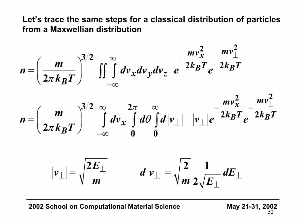
Let’s trace the same steps for a classical distribution of particlesfrom a Maxwellian distribution
2002 School on Computational Material Science May 21-31, 2002
22
22
3 22 2
3 2 22 2
0 0
2
2
2 2 12
xB B
xB B
mvmvk T k T
x y zB
mvmvk T k T
xB
mn dv dv dv e ek T
mn dv d d v v e ek T
Ev d v dEm m E
π
π
θπ
⊥
⊥
∞ − −
−∞
∞ ∞ − −
⊥ ⊥−∞
⊥⊥ ⊥ ⊥
⊥
=
=
= =
∫∫ ∫
∫ ∫ ∫

53
After changing variables
2002 School on Computational Material Science May 21-31, 2002
( )( )
3 2
0
3 2
0
3 2
00 exp 0
2 2 122 2
22
22
xB
xB
xB
B B
E Ek T
xB
E Ek T
xB
E Ek T
x BB
k T E k T
m En dv dE ek T m m E
mn dv dE ek T m
mn dv k T ek T m
ππ
ππ
ππ
⊥
⊥
⊥
−∞ ∞ −⊥
⊥⊥−∞
−∞ ∞ −
⊥−∞
∞−∞ −
−∞
− − +
=
=
= −
∫ ∫
∫ ∫
∫

54
Finally
2002 School on Computational Material Science May 21-31, 2002
2
2
2 2
3 22
1 22
1 2 1 202 2
0negative positive
22
2
2 2
x
B
x
B
x x
B B
x x
mv
k TBx
B
mv
k Tx
B
mv mv
k T k Tx x
B B
v v
m k Tn dv e
k T m
mn dv e
k T
m mn dv e dv e
k T k T
π
π
π
π π
−∞
−∞
−∞
−∞
− −∞
−∞
=
=
= +
∫
∫
∫ ∫

55
Here are the injecting distributions for the two cases
2002 School on Computational Material Science May 21-31, 2002
0
21 2
22 x
xB
mvk Tn dv
Bm ek Tπ
∞ − =
∫
2 2 0 log 1 exp2
B F xx
B
m k T E En dkk Tπ
∗ ∞ −= +
∫
56
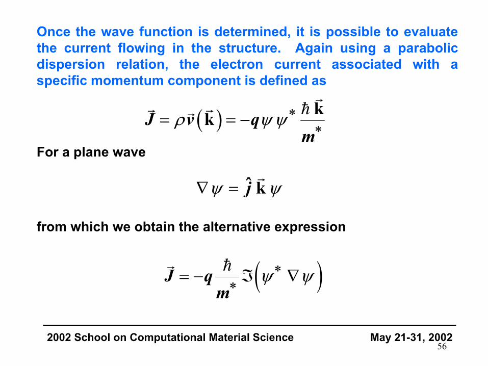
Once the wave function is determined, it is possible to evaluatethe current flowing in the structure. Again using a parabolicdispersion relation, the electron current associated with aspecific momentum component is defined as
For a plane wave
from which we obtain the alternative expression
2002 School on Computational Material Science May 21-31, 2002
( ) kkJ v qm
ρ ψ ψ ∗∗= = −
ˆ kjψ ψ∇ =
( )J qm
ψ ψ∗∗= − ℑ ∇

57
The continuity equation for electrons has the form
where
From Schrödinger equation
2002 School on Computational Material Science May 21-31, 2002
2q J
t tψρ ∂∂
= − = −∇ ⋅∂ ∂
2
t t tψ ψ ψψ ψ
∗∗∂ ∂ ∂
= +∂ ∂ ∂
( )
22
2 2 2
ˆ 1 ( )ˆ2ˆ ˆ1 ( )ˆ2 2
j V rt jm
j jV rjm m
ψψ ψ ψ
ψ ψ ψ ψ ψ ψ ψ
∗∗
∗ ∗ ∗ ∗∗ ∗
∂ = ∇ + ∂
− ∇ + = ∇ − ∇

58
Then, since
we have
and from the continuity equation itself
we get yet another expression for the current density
2002 School on Computational Material Science May 21-31, 2002
( ) 2ψ ψ ψ ψ ψ ψ∗ ∗ ∗∇ ⋅ ∇ = ∇ + ∇ ⋅∇
( )2 ˆ
2j
t mψ
ψ ψ ψ ψ∗ ∗∗
∂= ∇ ⋅ ∇ − ∇
∂
2q J
t tψρ ∂∂
= − = −∇ ⋅∂ ∂
( )ˆ
2j qJm
ψ ψ ψ ψ∗ ∗∗= ∇ − ∇
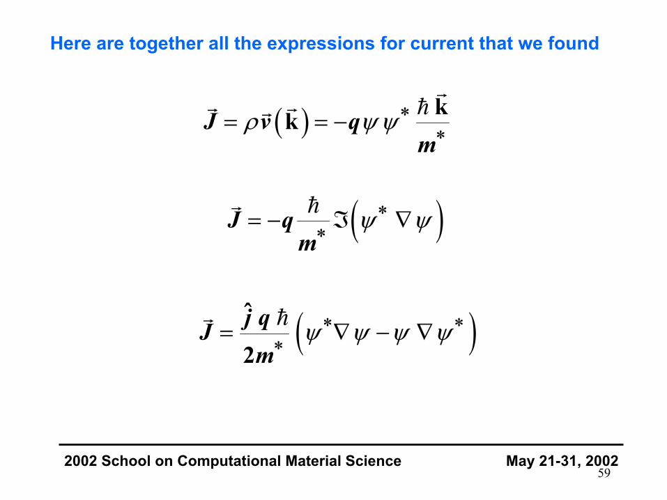
59
Here are together all the expressions for current that we found
2002 School on Computational Material Science May 21-31, 2002
( )ˆ
2j qJm
ψ ψ ψ ψ∗ ∗∗= ∇ − ∇
( ) kkJ v qm
ρ ψ ψ ∗∗= = −
( )J qm
ψ ψ∗∗= − ℑ ∇
60
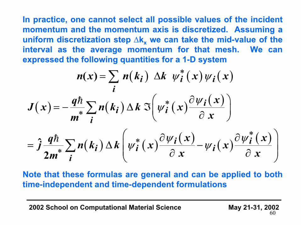
In practice, one cannot select all possible values of the incidentmomentum and the momentum axis is discretized. Assuming auniform discretization step ∆kx we can take the mid-value of theinterval as the average momentum for that mesh. We canexpressed the following quantities for a 1-D system
Note that these formulas are general and can be applied to bothtime-independent and time-dependent formulations
2002 School on Computational Material Science May 21-31, 2002
( ) ( ) ( )( ) i i ii
n x n k k x xψ ψ∗= ∆∑
( ) ( ) ( ) ( )
( ) ( ) ( ) ( ) ( )ˆ2
ii i
i
i ii i i
i
xqJ x n k k xxm
x xqj n k k x xx xm
ψψ
ψ ψψ ψ
∗∗
∗∗
∗
∂ = − ∆ ℑ ∂
∂ ∂= ∆ − ∂ ∂
∑
∑

61
Possible discussion items:
What can we do to formulate boundary conditions when quasi-equilibrium is not a good assumption?
How can we formulate a self-consistent simulation?
Video animation: Switching in a quantum nanostructure
2002 School on Computational Material Science May 21-31, 2002

62
1D quantum simulation using transmission line theory
Consider a single barrier system
The wave function can be written as
2002 School on Computational Material Science May 21-31, 2002
( ) ( ) ( )[ ]
( )( )2ˆ ˆ 2
amplitude reflecti
exp ex
on coeff
p
icient
j j m E V
x A x x
γ
ψ γ Γ γ
α β
Γ
∗= +
− −
= −
=
=
x
V2
V1

63
The system behaves like a standard transmission line
2002 School on Computational Material Science May 21-31, 2002
( ) ( ) ( )[ ]
( )( )
( ) ( )
( )( )
1 1 1 1
2
2 2 2
22
1 1 1
2 2
exp
ˆ 2
exp exp
ˆ 2
x A x x
j m E V
x A x
j m E V
ψ γ Γ γ
ψ γ
γ
γ ∗
∗
= − −
=
=
=
−
−
x
V2
V1
region 1 region 2
0

64
By applying continuity conditions, we obtain Γ
Then, we define the following auxiliary function
2002 School on Computational Material Science May 21-31, 2002
( ) ( ) ( ) ( )[ ]11 1 1exp exp1
xx x
dx Ad xj m j m
ψγ γ Γ γφ −∗ ∗= = +
( ) ( )
( ) ( )
( ) ( )( ) ( )
1 2
1 21 2
2 2 1 1
2 2 1 1
0 01 10 0d d
d x d xm m
m m
m m
ψ ψ
ψ ψ
γ γΓ
γ γ
∗ ∗
∗ ∗
∗ ∗
=
=
−⇒ =
+

65
This function is anologous to electric voltage in a transmissionline
The wave function is analogous to electric current in atransmission line
and the scaling factor behaves like characteristic impedance
2002 School on Computational Material Science May 21-31, 2002
( ) ( ) ( )[ ]1 1 1exp exp1 x xx Aj m
γ γ Γ γφ −∗= +
( ) ( ) ( )[ ]1 1 1 1exp expx A x xψ γ Γ γ= − −
10Zj m
γ∗=

66
The probability current flow density is analogous to time averagepower in a transmission line
At any location one can define the line impedance as
Indicate the load impedance as ZL = Z2 the input impedance of thesystem is
2002 School on Computational Material Science May 21-31, 2002
( ) { }1ˆ 22
Jq j m
ψ ψ ψ ψ φ ψ∗ ∗ ∗∗= ∇ − ∇ = ℜ
( ) ( )( )x
Z xx
φψ
=
2 00
0 2
cosh( ) sinh( )cosh( ) sinh( )
where
in
in
Z L Z LZ ZZ L Z L
x L
γ γγ γ
−=
−
= −

67
If a system consists of a sequence of different material layers,each layer can be treated as a transmission line with differentcharacteristic impedance, which depends on the effective mass.The reflection coefficient of the structure can be obtained withthe same algebra of transmission lines.
Possible discussion items:
What are the limitations of this approach?How can we include bias and self-consistency?
2002 School on Computational Material Science May 21-31, 2002
Z01 Z01 Z01
Z02 Z02

68
2D Solution with iterative tight-binding Green’s functions.Let’s assume a 2-D electron gas system define by a wave guidelike pattern, and perform a uniform discretization (tight-bindinglattice). Assume a flat potential floor for simplicity. We arelooking for the structure’s reflection and transmissioncoefficients.
2002 School on Computational Material Science May 21-31, 2002
+ ++ +
Gji
Gii
i j
69
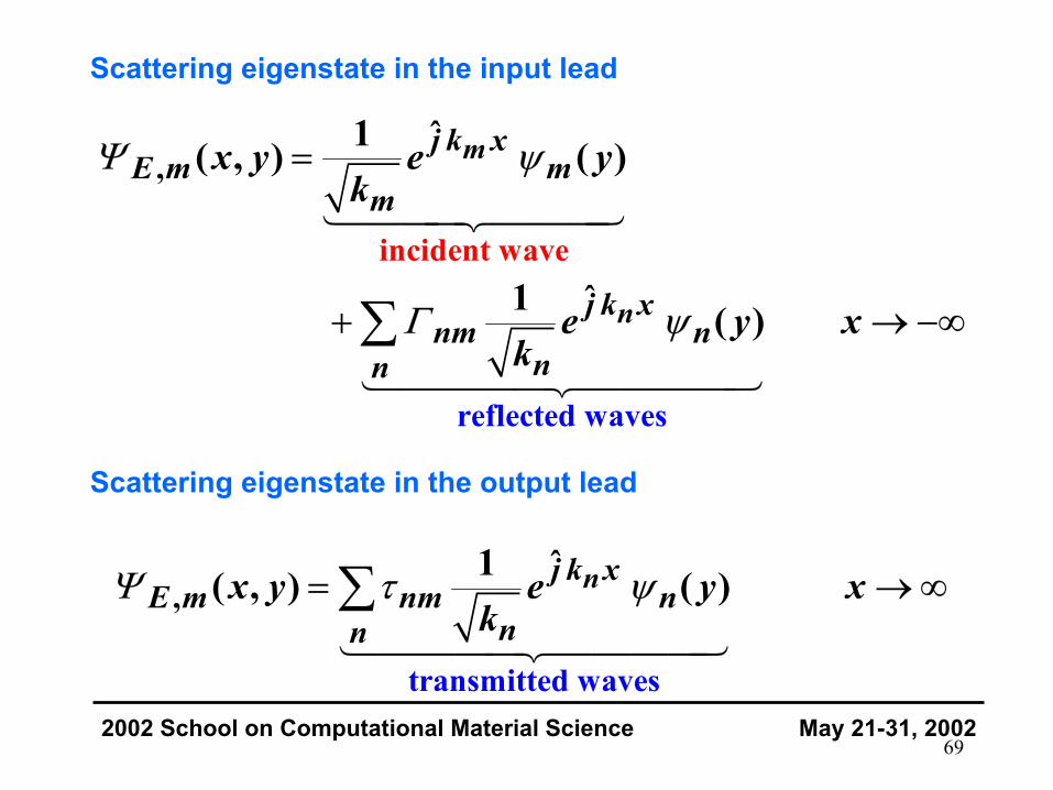
Scattering eigenstate in the input lead
Scattering eigenstate in the output lead
2002 School on Computational Material Science May 21-31, 2002
incid
reflected
ent wave
w
,
av
ˆ
s
ˆ
e
1( , ) ( )
1 ( )
m
n
j k xE m m
m
j k xnm n
nn
x y e yk
e y xk
Ψ ψ
Γ ψ
=
+ → −∞∑
tra
ˆ,
nsmitted waves
1( , ) ( )nj k xE m nm n
nnx y e y x
kΨ τ ψ= → ∞∑

70
Start with output lead as an isolated section
2002 School on Computational Material Science May 21-31, 2002
jq+1
hard walls
semi-infinite chain
jq+1
Gj,q+1B
Gq+1,q+1B
B

71
The Green’s function is a matrix [ n × n ] where “n” is the numberof modes in the trasverse chain (same as the number ofdiscretization nodes, 3 in the example)
2002 School on Computational Material Science May 21-31, 2002
1 Energy above cut-off
1 Energy below cut-off
cos ˆ2
cosh ˆ2
EV
EV
θ
α
−
−
=
=
E1
E2
E3 1
2q+1, q+13
j, q+1
0 00 00 0
GG
G
E

72
Green’s functions for the semi-infinite chain
2002 School on Computational Material Science May 21-31, 2002
( )
( )
( )
( )
ˆB above cut-offq+1,q+1
B below cut-offq+1,q+1
ˆ j-qB above cut-offj,q+1
j-qB below cut-offj,q+1
= ˆ
= ˆ
= ˆ
= ˆ
ji
i
j
i
i
eGV
eGV
eGV
eGV
θ
α
θ
α
−
−

73
Then, treat the next section as an isolated finite chain
2002 School on Computational Material Science May 21-31, 2002
qp
hard walls
finite chain
qp
Gq,pA
Gp,pA
A
74 2002 School on Computational Material Science May 21-31, 2002
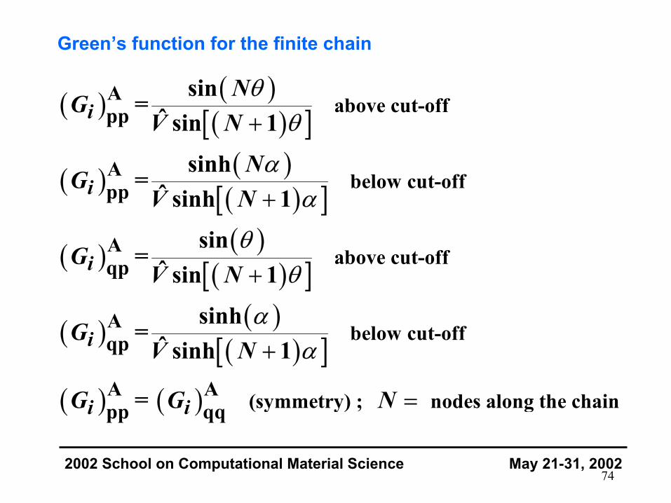
Green’s function for the finite chain
( ) ( )( )[ ]
( ) ( )( )[ ]
( ) ( )( )[ ]
( ) ( )( )[ ]
( ) ( )
A above cut-offpp
A below cut-offpp
A above cut-offqp
A below cut-offqp
A A (symmetry) ; nodes along the chainpp qq
sin= ˆ sin 1
sinh= ˆ sinh 1
sin= ˆ sin 1
sinh= ˆ sinh 1
=
i
i
i
i
i i
NG
V N
NG
V N
GV N
GV N
G G N
θθ
αα
θθ
αα
+
+
+
+
=

75 2002 School on Computational Material Science May 21-31, 2002
GA is a matrix [ m × m ] where m is the number of transversemodes (number of transverse discretization nodes)
1
2
1
0 0 0 0 0
0 0 0 0 0
0 0 0 0 0
0 0 0 0 0
0 0 0 0 0
0 0 0 0 0
A
A
Am
Am
G
G
G
G
−
i
i
E
In wider section, moremodes are above cut-off
A B

76 2002 School on Computational Material Science May 21-31, 2002
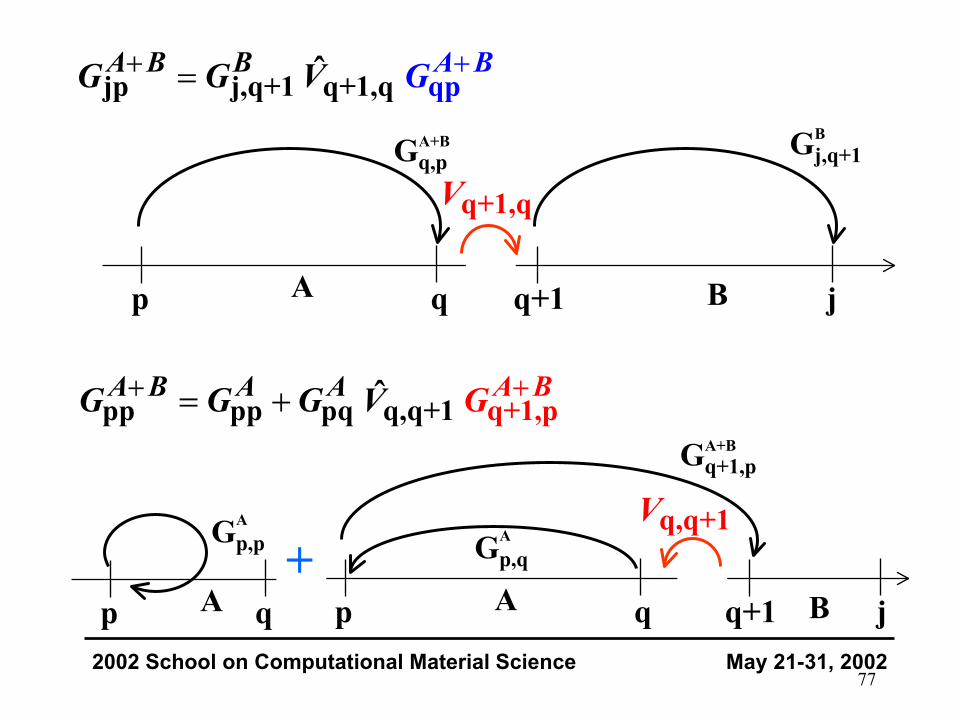
Now, add sections A and B - Application of Dyson’s equation
jp
Gj,pA+B
GppA+B
A+B
qp
Gq,pA
Gp,pA
A jq+1
Gj,q+1B
Gq+1,q+1B
B+V̂
totalHamiltonian
Dyson's equation f
connectionsisolated regio
or the Green's functio
ns
n
0
0 0
ˆ
ˆ
H H V
G G G V G
= +
= +
77 2002 School on Computational Material Science May 21-31, 2002
jp j,q+ q1 q p+1,qˆA B B A BG G GV+ +=
qp
Gq,pA+B
A jq+1
Gj,q+1B
B
q+1,qV
pp pp pq q,q+1 q+1,pˆA B A A BAG G GG V ++ = +
qp
Gq+1,pA+B
A jq+1 B
q,q+1V
qp A
Gp,pA
+ Gp,qA

78 2002 School on Computational Material Science May 21-31, 2002
q+1,q+q+1, 1 q+1,q qpp ˆA B B A BG V GG + +=
qp
Gq,pA+B
A jq+1
Gq+1,q+1B
B
q+1,qV
qp qq q,q+1 1,q q pp +ˆB A A BA AG VG G G ++ = +
qp
Gq+1,pA+B
A jq+1 B
q,q+1V
qp A
Gq,pA
+Gq,q
A

79 2002 School on Computational Material Science May 21-31, 2002
Add sections A and B
( )
jp j,q+1 q+1,q qp
pp pp pq q,q+1 q+1,p
qp qp qq q,q+1 q+1,p
q+1,p q+1,q+1 q+1,q qp
qp qp qq q,q+1 q+1,q+1 q+1,q qp
qq q,q+1 q+1,q+1 q+1,q
ˆ
ˆ
ˆ
ˆ
ˆ ˆ
ˆ ˆ1
A B B A B
A B A A A B
A B A A A B
A B B A B
A B A A B A B
A B
G G V G
G G G V G
G G G V G
G G V G
G G G V G V G
G V G V G
+ +
+ +
+ +
+ +
+ +
=
= +
⇒ = +
⇒ =
= +
−
( ) 1qp qq q,q+1 q+1,q+1 q+1
qp qp
,q qpˆ ˆ1
A B A
A B A B AG G V G G
G
V+
+
−⇒ =
=
−

80 2002 School on Computational Material Science May 21-31, 2002
Get the first Green’s function for the coupled system
( )
Self-energy for the transverse chain at locat
1
jp j,q+1 q+1,q qq q,q+1 q+1,q+1 q+1,q qp
1q
jp j,q+1 q+1
p qq q,q+1 q+1,q+1 q+1,q p
q
q
,q p
ˆ ˆ ˆ1
ˆ
ˆ ˆ
1
Bq
A B B A B A
S
A B B A B
A
B
B
q
A B A
G G V G V G V G
G G V G
S
G G V G V G
−
+
−+
+ +
= −
⇓
= −
=
= ion q, due to presence of B

81 2002 School on Computational Material Science May 21-31, 2002
Get the second Green’s function for the coupled system
( )
( )
( )
1q+1,p q+1,q+1 q+1,q
pp
1pp pq q
qq qp
pp pq q,q+1 q+1,p
q qpq,q+1 q+1,q
q+1,p q+1,q+1 q+1,q qp
+1
1qp qq
q q
p
,
q
+1
ˆ 1
1
ˆ
ˆ
ˆ
1
ˆ
A B B A B A
A B
A A A B Aq
B
q
A
q
A A B
A B A B Aq
A B B A
S
B
B
G
G G G S G
G G V G S G
G G V G
V
G G V G
G G S
G V
G
−
+
−
+
+
+ +
−+
+
= −
= +
−
=
=
⇓
=
−

82 2002 School on Computational Material Science May 21-31, 2002
Here are the Green’s function results we were looking for
( )( ) 1
pp pp pq qq qp
1jp j,q+1 q+1,
.. ..
pp q
q qq qp
+1,p
1
and are diagonal matrices
and are non-diagonal matr
ˆ 1
ices
A B A A B A B Aq q
A
A B B A B
B
A A
q
B
A
B
G G G
G
S
G
G S G
NOTE
G G V G S G
G G
−+
+ +
−+
+ −
= −
=

83 2002 School on Computational Material Science May 21-31, 2002
Example of coupling matrices
1, 3 3 modes on section q+1
1, 7 7 modes on section q
n
m
= Æ
= Æ
q+1q
Here is [ 3 3 ]
BG¥
Here is [ 7 7 ]
AG¥
q,q+1
q+1,q
q,q+1 q+1,q
is [ 7 3 ]
is [ 3 7 ]
T
V
V
V V
¥
¥
= È ˘Î ˚
( ) ( ) ( )q,q+1
Overlap integral
ˆ n mnml
V V l ly y*= Â Â

84 2002 School on Computational Material Science May 21-31, 2002
Transverse Eigenvalues and Eigenfunctions
The simplest approach is to use an infinite square well model for thetransverse direction. But one could also solve a 2-D self-consistentSchrödinger/Poisson solution on the cross section and feed theeigenenergies and eigenfunctions (wave functions) to the Green’sfunction code. The tight-binding model gives as many eigevalues asnodes. Typically, 20 nodes are sufficient to resolve realistic structures.
E2
2
2 1 0 0 0 0
1 2 1 0 0 0
0 1 0 012 0 0 1 0( )
0 0 0 1 2 1
0 0 0 0 1 2
m x∆
−
− −
−
−
− −
−
i i
i i
Discretized Hamiltonian with V(x) = 0(flat potential)
L

85 2002 School on Computational Material Science May 21-31, 2002
Transverse Eigenvalues
[ ]2
2
2
2
2 2 2
2 2
1
2 ( )
1
2 ( )
2 2 2 2 21 12 2 2 2 22 2 2( ) ( )
0 0 2 cos1
01,
0
0 0 2; 1;
2 2cos1
Continuum model
( )
( 1)
n
m x
nm x
nm m mx x
na b E a bcN
c a bn N
c a b
c a a b c
nE
N
n xE
L L n N n
∆
∆
∆ ∆
πγ
γ
γ
π
π π ∆ π
= ++
⇒ ∈
= = = − =
= −+
= = =+

86 2002 School on Computational Material Science May 21-31, 2002
Transverse Eigenfunctions
Hard walls, zero wave function at the wall.
( )( )( )( )
( ) sin1
1ˆ1 exp 2 11ˆ2 2 1 exp 2 1
n n
n
n m nm
n ll AN
Aj n N NNj n N
πψ
π
π
ψ ψ δ
= +
= − +
+ ℜ − +
=
87 2002 School on Computational Material Science May 21-31, 2002
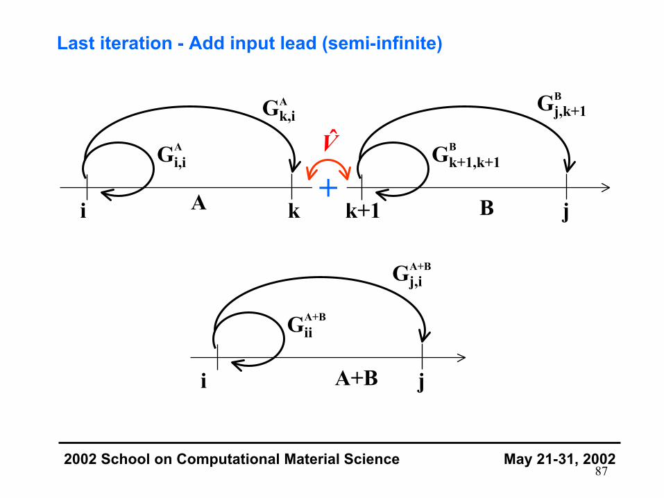
Last iteration - Add input lead (semi-infinite)
Gj,iA+B
ji
GiiA+B
A+B
ki
Gk,iA
Gi,iA
A jk+1
Gj,k+1B
Gk+1,k+1B
B+V̂

88 2002 School on Computational Material Science May 21-31, 2002
Last iteration - Add input lead (semi-infinite)
( )( ) ( )[ ]
( )( ) ( )[ ]
( )( )
( )( )
ˆ i-k-1A above cut-offi,i
i-k-1A below cut-offi,i
ˆ i-k-1A above cut-offk,i
i-k-1B below cut-offk,i
sin i-k-1= ˆ sin
sinh i-k-1= ˆ sinh
= ˆ
= ˆ
j
i
i
j
i
i
eGV
eGV
eGV
eGV
θ
α
θ
α
θθ
αα
−
−

89 2002 School on Computational Material Science May 21-31, 2002
With the application of the same algorithm obtain
Gj,iA+B
ji
GiiA+B
A+B
ABi,i
ABj,i
= [ m m ] matrix (m = nodes in input lead)
gives the reflection coefficients
= [ n n ] matrix (n = nodes in output lead)
gives the transmission coefficients
G
G
×
×

90 2002 School on Computational Material Science May 21-31, 2002
Reflection and transmission coefficients are evaluated for allmodes in the input and output leads
( )
( )
( )
ji
ii
ˆ i j, ji
elementof
ˆ 2 i,
iielementof
refle
transmission coeffic
ˆ ˆ2 sin sin
sin si
ction coeffic
n
ˆ ˆ2 sin
ie
ie ts
n s
n
t
m n
m n
jm n n m
G
jm n n m
m nm
G
j V e n G m
e
j V n G m
θ θ
θ θ
τ θ θ
Γ θ θ
θ δ
−
+
= −
= −
× +
1 for
0 for nmm n
m nδ
==
≠
91 2002 School on Computational Material Science May 21-31, 2002
Possible discussion items:
How to include realistic structures?
Quasi-3D simulation
Full self-consistent 3-D simulation
Available Software: TBGreen code

92 2002 School on Computational Material Science May 21-31, 2002
Mode-matching method
The structure is partitioned into slices in which the potentialprofile is constant along the longitudinal direction.
A 1-D Schrödinger equation is solved in each section toobtain transverse eigenmodes and eigenvalues.
The continuity of the wavefunction and of its normalderivative is enforced at each interface between differentsections.
The equations are then projected onto appropriate sets oftransverse modes and solved using numerical procedures.

93 2002 School on Computational Material Science May 21-31, 2002
Mode-matching method (2-D electron gas)
xy
( ) ( ) ( )
( )
( )
( )
ˆ
2 22 2
,
1
2 sin
2 2
x
n nn
j k xn
n
y
nx y n
x y a x n
x ek
nk yn
L L
kk k Em m
ψ ϕ χ
ϕ
χ
±
∗ ∗
=
=
=
+ = =
∑
94 2002 School on Computational Material Science May 21-31, 2002
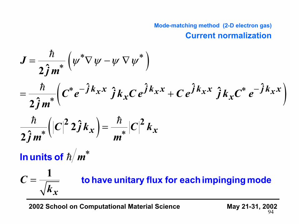
Mode-matching method (2-D electron gas)
Current normalization
( )
( )( )
ˆ ˆ ˆ ˆ
2 2
ˆ2
ˆ ˆˆ2
ˆ2ˆ2
1
x x x xj k x j k x j k x j k xx x
x x
x
Jj m
C e j k C e C e j k C ej m
C j k C kj m m
m
Ck
ψ ψ ψ ψ∗ ∗∗
− −∗ ∗∗
∗ ∗
∗
= ∇ − ∇
= +
=
= to have unitary flux for each impinging mode
In units of
95 2002 School on Computational Material Science May 21-31, 2002
Mode-matching method (2-D electron gas)
NM
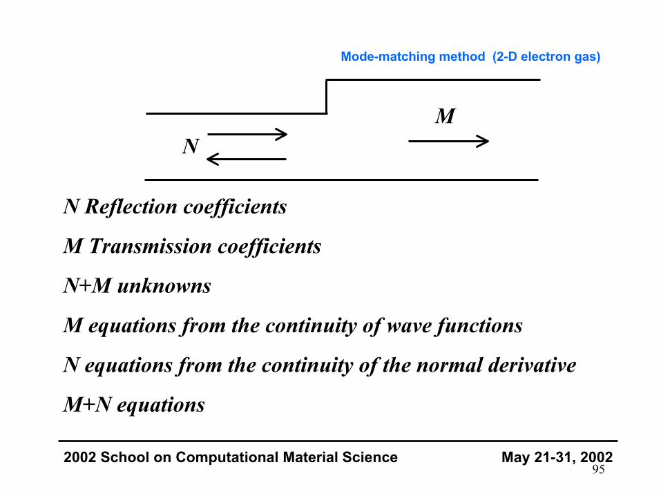
N Reflection coefficients
M Transmission coefficients
N+M unknowns
M equations from the continuity of wave functions
N equations from the continuity of the normal derivative
M+N equations

96 2002 School on Computational Material Science May 21-31, 2002
Mode-matching method (2-D electron gas)
Leftmost interface ( x = xA )
( ) ( )
( ) ( )
( ) ( )
( ) ( )
ˆ ˆ
ˆ ˆ
ˆ ˆ
ˆ ˆ
1 1
1 1
ˆ
ˆ ˆ
i A n A
m A m A
i A n A
m A m A
j k x j k xi n n
i nn
j x j xm m m m
m mm m
j k x j k xi i n n n
nj x j x
m m m m m mm m
e y R e yk k
c e y d e y
k e y j R k e y
j c e y j d e y
ν ν
ν ν
ψ ψ
χ χν ν
ψ ψ
ν χ ν χ
−
−
= −
+ +
=
+ −
∑
∑ ∑
∑
∑ ∑
97 2002 School on Computational Material Science May 21-31, 2002
Mode-matching method (2-D electron gas)
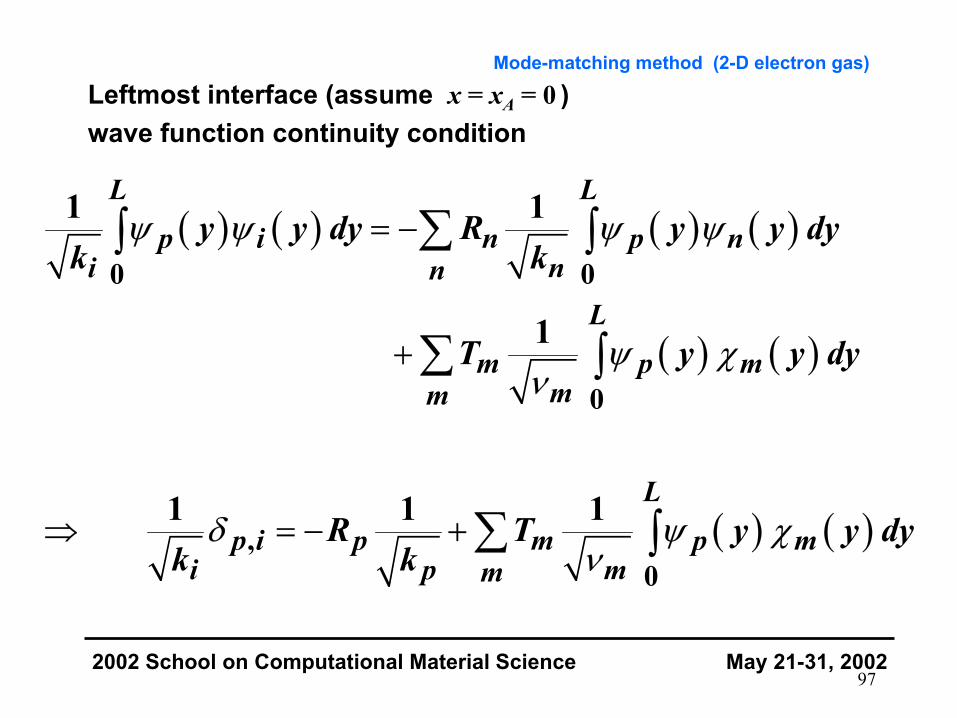
Leftmost interface (assume x = xA = 0 )wave function continuity condition
( ) ( ) ( ) ( )
( ) ( )
( ) ( )
0 0
0
,0
1 1
1
1 1 1
L L
p i n p ni nn
L
m p mmm
L
p i p m p mi p mm
y y dy R y y dyk k
T y y dy
R T y y dyk k
ψ ψ ψ ψ
ψ χν
δ ψ χν
= −
+
⇒ = − +
∑∫ ∫
∑ ∫
∑ ∫

98 2002 School on Computational Material Science May 21-31, 2002
Mode-matching method (2-D electron gas)
Leftmost interface (assume x = xA = 0 )derivative continuity condition
( ) ( ) ( ) ( )
( ) ( )
( ) ( )
( ) ( )
' '
0 0'
0'
0'
0
ˆ ˆ
ˆ
ˆ
ˆ ˆ
L L
i p n n n p nn
L
m m p mm
L
i p n
L
n n p n p pn
j k y y dy j R k y y dy
j T y y dy
j k y y dy
j R k y y dy j T
χ ψ χ ψ
ν χ χ
χ ψ
χ ψ ν
=
+
⇒ =
+
∑∫ ∫
∑ ∫
∫
∑ ∫