Embed Size (px)
Citation preview
Preprint typeset in JHEP style - HYPER VERSION hep-th/0703057
SU-ITP-07/01Imperial/TP/07/TW/01
Numerical Kahler-Einstein metric on the third del Pezzo
Charles Doran
Department of Mathematics, University of Washington, Seattle, WA 98195-1560, [email protected]
Matthew Headrick
Stanford Institute for Theoretical Physics, Stanford, CA 94305-4060, [email protected]
Christopher P. Herzog
Department of Physics, University of Washington, Seattle, WA 98195-1560, [email protected]
Joshua Kantor
Department of Mathematics, University of Washington, Seattle, WA 98195-1560, [email protected]
Toby Wiseman
Blackett Laboratory, Imperial College London, London SW7 2AZ, [email protected]
Abstract: The third del Pezzo surface admits a unique Kahler-Einstein metric, which is notknown in closed form. The manifold’s toric structure reduces the Einstein equation to a singleMonge-Ampere equation in two real dimensions. We numerically solve this nonlinear PDEusing three different algorithms, and describe the resulting metric. The first two algorithmsinvolve simulation of Ricci flow, in complex and symplectic coordinates respectively. Thethird algorithm involves turning the PDE into an optimization problem on a certain spaceof metrics, which are symplectic analogues of the “algebraic” metrics used in numerical workon Calabi-Yau manifolds. Our algorithms should be applicable to general toric manifolds.Using our metric, we compute various geometric quantities of interest, including Laplacianeigenvalues and a harmonic (1, 1)-form. The metric and (1, 1)-form can be used to constructa Klebanov-Tseytlin-like supergravity solution.

Contents
1. Introduction 2
2. Gauge/gravity duality 4
3. Mathematical background 63.1 Complex and symplectic coordinates 63.2 Boundary conditions and the canonical metric 83.3 Examples 93.4 The Monge-Ampere equation 103.5 Volumes 123.6 The Laplacian 123.7 Harmonic (1, 1)-forms 133.8 More on dP3 14
4. Ricci flow 154.1 Complex coordinates 174.2 Symplectic coordinates 184.3 Results 194.4 Laplacian eigenvalues 20
5. Symplectic polynomials 24
6. Constrained optimization 276.1 Laplacian eigenvalues 306.2 Harmonic (1,1)-forms 31
7. Discussion 33
A. Canonical metric on CP2 34
B. Numerical Ricci flow implementation and error estimates 35B.1 Implementation in complex coordinates 35B.2 Implementation in symplectic coordinates 36B.3 Simulation of Ricci flow 36B.4 Convergence tests 37
C. D6-invariant polynomials 39
– 1 –

D. Convergence and error estimates of the constrained optimization method 40
1. Introduction
Kahler metrics on manifolds play an important role in mathematics and physics. As Yaudemonstrated [1], in the Kahler case it is often possible to prove the existence (or nonexistence)of metrics which solve the Einstein equation. While it is extremely valuable to know whetherthey exist, for many purposes one also wants to know their specific form. The existencetheorems, however, are generally non-constructive, and explicit examples of Kahler-Einsteinmetrics are rare. This state of affairs naturally leads to the following question: Is it possible,in practice, to find accurate numerical approximations to these metrics using computers? Thelast two years have seen significant success, with a variety of different algorithms providingnumerical solutions to the Einstein equation on the Calabi-Yau surface K3 [2–4] and on athree-fold [5]. The Kahler property proved to be as crucial for this numerical work as it wasfor the existence theorems.
In this paper we extend this success to a non-Calabi-Yau manifold, namely CP2 blown upat three points (CP2#3CP2), also known as the third del Pezzo surface (dP3). This manifoldis known by work of Siu [7] and Tian-Yau [6] to admit a Kahler-Einstein metric with positivecosmological constant, but as in the Calabi-Yau case that metric is not known explicitly. Animportant property of dP3 that differentiates it from Calabi-Yau manifolds is that it is toric.Toric manifolds are a special class of Kahler manifolds whose U(1)n isometry group (where nis the manifold’s complex dimension) allows even greater analytical control, and we developalgorithms for solving the Einstein equation that specifically exploit this structure. We shouldalso note that the Kahler-Einstein metric on dP3 is unique (up to rescaling); therefore, ratherthan having a moduli space of metrics as we have in the case of Calabi-Yau manifolds, thereis only one metric to compute.
On the physics side, the Kahler-Einstein metric on dP3 is important because it can beused to construct an example of a gauge/gravity duality. These dualities provide a bridgebetween physical theories of radically different character, allowing computation in one theoryusing the methods of its dual. Given the Kahler-Einstein metric on dP3, one can construct afive-dimensional Sasaki-Einstein metric. Compactifying type IIB supergravity on this man-ifold one obtains an AdS5 supergravity solution, which has a known superconformal gaugetheory dual [8–10]. An interesting generalization includes a 3-form flux from wrapped D5-branes. This flux can be written in terms of a harmonic (1, 1)-form on dP3, which we alsocompute numerically in this paper. The resulting supergravity solution (the analogue of theKlebanov-Tseytlin solution on the conifold [11]) is nakedly singular, but is the first step to-ward finding the full supergravity solution on the smoothed-out cone (the analogue of theKlebanov-Strassler warped deformed conifold [12]). This smoothed-out cone is dual to a
– 2 –

cascading gauge theory, and knowing the explicit form of the supergravity solution wouldbe useful for both gauge theory and cosmology applications. This physics background isexplained in detail in Section 2.
In Section 3, we review the mathematical background necessary for understanding therest of the paper. Here we closely follow the review article on toric geometry by Abreu [13].We explain the two natural coordinate systems on a toric manifold, namely complex andsymplectic coordinates. In complex coordinates, the metric is encoded in the Kahler potential,and in symplectic coordinates in the symplectic potential; these two functions are relatedby a Legendre transform. In either coordinate system, the Einstein equation reduces to asingle nonlinear partial differential equation, of Monge-Ampere type, for the correspondingpotential. Thanks to the U(1)n symmetry, this PDE is in half the number of dimensions ofthe original manifold (two real dimensions for dP3). In this section we also derive the equationwe need for the (1, 1)-form, and give all the necessary details about dP3.
In this paper we describe three different methods to solve the Monge-Ampere equation.In Section 4 we explain the first two methods, which involve numerically simulating Ricci flowin complex and symplectic coordinates respectively. Specifically, we use a variant of Ricci flow(normalized) that includes a Λ term,
∂gµν∂t
= −2Rµν + 2Λgµν , (1.1)
whose fixed points are clearly Einstein metrics with cosmological constant Λ. According toa recent result of Tian-Zhu [14], on a manifold which admits a Kahler-Einstein metric, theflow (4.1) converges to it starting from any metric in the same Kahler class. Our simulationsbehaved accordingly, yielding Kahler-Einstein metrics accurate (at the highest resolutionswe employed) to a few parts in 106 (and which agree with each other to within that error).Numerical simulations of Ricci flow have been studied before in a variety of contexts [15–17],but as far as we know this is the first time they have been used to find a new solution to theEinstein equation (aside from a limited exploration of its use on K3 [2]). In this section wealso explore the geometry of this solution, and discuss a method for computing eigenvaluesand eigenfunctions of the Laplacian in that background.
In Section 5 we introduce a different way to represent the metric, based on certain poly-nomials in the symplectic coordinates. This non-local representation is a symplectic analogueof the “algebraic” metrics on Calabi-Yau manifolds employed in numerical work by Donald-son [3] and Douglas et al. [4, 5]. To demonstrate the utility of this representation we give alow order polynomial fit to the numerical solutions found by Ricci flow, that can be writtenon one line and yet agrees with the true solution to one part in 103, and everywhere satisfiesthe Einstein condition to better than 10%.
In Section 6 we discuss our third method to compute the Kahler-Einstein metric. Asabove we represent the metric using polynomials in the symplectic coordinates, but now weconstrain the polynomial coefficients by solving the Monge-Ampere equation order by order inthe coordinates. This leaves a small number of undetermined coefficients, which we compute
– 3 –
by minimizing an error function. Using this method we obtain numerical metrics of similaraccuracy to those found by Ricci flow. By a similar method we also calculate eigenvalues andeigenfunctions of the Laplacian, and the harmonic (1, 1)-form.
We conclude the paper with a brief discussion of the three methods and their relativemerits in Section 7.
At the two websites [21], we have made available for download the full numerical datarepresenting our metrics, as well as Mathematica notebooks that input the data and allowthe user to work with those metrics. The codes used to generate the data are also availableon those websites.
We believe that all of the methods we present here can be applied to a general toricmanifold. We will report elsewhere on an application to dP2 [18], which does not admit aKahler-Einstein metric but does admit a Kahler-Ricci soliton [19]. For future work, thereis also a natural analogue of dP3 to study in three complex dimensions. From Batyrev’sclassification of toric Fano threefolds, it follows that there are precisely two of them that admitKahler-Einstein metrics which are not themselves products of lower dimensional manifolds [20,Section 4]. One of these is CP3. The other is the total space of the projectivization of therank two bundle O ⊕ O(1,−1) over CP1 × CP1. Its Delzant polytope (see Section 3 for thedefinition) possesses a D4 symmetry, and a fundamental region is simply a tetrahedron.
While this work was in progress we have learned that Kahler-Einstein metrics on dP3
have also been computed in [22] using the methods of [3].
2. Gauge/gravity duality
A prototypical example of a gauge/gravity duality which provides the physics motivationfor studying dP3 is the Klebanov-Strassler (KS) supergravity solution [12]. (Mathematiciansmay wish to skip this section.) The KS solution is a solution of the type IIB supergravityequations of motion. The space-time is a warped product of Minkowski space R1,3 and thedeformed conifold X. The affine variety X has an embedding in C4 defined by
4∑i=1
z2i = ε (2.1)
where zi ∈ C. There are also a variety of nontrivial fluxes in this solution which we will returnto later.
One important aspect of the KS solution is its conjectured duality to a non-abelian gaugetheory, namely the cascading SU(N) × SU(N + M) N = 1 supersymmetric gauge theorywith bifundamental fields Ai and Bi, i = 1 or 2, and superpotential
W = εijεklAiBkAjBl . (2.2)
This theory is similar in a number of respects to QCD; it exhibits renormalization groupflow, chiral symmetry breaking, and confinement. Moreover, all of these properties can beunderstood from the dual gravitational perspective.
– 4 –

In addition to its gauge theory applications, the KS solution is important for cosmology.Treating the deformed conifold as a local feature of a compact Calabi-Yau manifold, the KSsolution provides a string compactification with a natural hierarchy of scales in which all thecomplex moduli are fixed [23]. Stabilizing the Kahler moduli as well [24], the KS solutioncan become a metastable string vacuum and thus a model of the real world. In this context,inflation might correspond to the motion of D-branes [25] and cosmic strings might be thefundamental and D-strings of type IIB string theory [26].
One naturally wonders to what extent the cosmological and gauge theoretic applicationsdepend upon the choice of the deformed conifold. A natural way to generalize X is to considersmoothings of other Calabi-Yau singularities. One such family of singularities involves aCalabi-Yau where a del Pezzo surface dPn shrinks to zero size. (Here dPn is CP2 blown upat n points.) Note we are distinguishing here between resolutions — or Kahler structuredeformations — where even dimensional cycles are made to be of finite size, and smoothings— complex structure deformations — where a three dimensional cycle is made finite. Usingtoric geometry techniques, Altmann [27] has shown that the total space of the canonicalbundle over dP1 admits no smoothings, while dP2 admits one and dP3 two.1 The higherdPn are not toric. Thus two relatively simple candidates for generalizing the KS solution aresmoothed cones over the complex surfaces dP2 and dP3.
Without knowing the details of the metric on the smoothed cone X, one can show thata generalization of the KS solution exists for such warped products [31]. The solution willhave a ten dimensional line element of the form
ds2 = h(p)−1/2ηµνdxµdxν + h(p)1/2ds2X , (2.3)
where ds2X is the line element on X, p ∈ X, the map h : X → R+ is called the “warp factor”,and ηµν is the Minkowski tensor for R1,3 with signature (−+ ++). There are also a varietyof nontrivial fluxes turned on in this solution. There is a five form flux
F5 = dC4 + ?dC4 , where C4 =1gsh
dx0 ∧ dx1 ∧ dx2 ∧ dx3 , (2.4)
and where gs is the string coupling constant. The finite smoothing indicates the presence ofa harmonic (2, 1)-form ω2,1 which we take to be imaginary self-dual: ?Xω2,1 = iω2,1. Fromω2,1 we construct a three-form flux G3 = Cω2,1 where C is a constant related to the rank ofthe gauge group in the dual theory. The warp factor satisfies the relation
4Xh = −g2s
12Gabc(G∗) fabc , (2.5)
where the indices on G3 are raised and the Laplacian4X is constructed using the line elementds2X without the warp factor. Although this solution holds for general X, clearly in order toknow detailed behavior of the fluxes and warp factor as a function of p, we need to know ametric on X.
1The physical relevance of this fact for supersymmetry breaking was pointed out in [28–30].
– 5 –
From this perspective, we have chosen to study dP3 and not dP2 in this paper becausedP3 is known to have a Kahler-Einstein metric [6] while dP2 does not [32]. Given that dP3 isKahler-Einstein, we can construct a singular Calabi-Yau cone over dP3 in a straightforwardmanner:
ds2X = dr2 + r2[(dψ + σ)2 + ds2V
], (2.6)
where σ = −2i(∂f − ∂f) and f is half the Kahler potential on V = dP3. Here ds2V is aKahler-Einstein line element on dP3. In a hopefully obvious notation, r is the radius of thecone and ψ an angle. Although such a cone over dP2 probably exists as well, it will involve anirregular Sasaki-Einstein manifold as an intermediate step; the metric on the Sasaki-Einsteinmanifold over dP2 is not yet known.
Given that dP3 is Kahler-Einstein, the problem of finding ω2,1 on the singular conereduces to finding a harmonic (1, 1)-form θ on dP3 such that θ ∧ ω = 0 (where ω is theKahler form on V ) and ?V θ = −θ, as pointed out in [33]. The relation between ω2,1 and θ isω2,1 = (−idr/r + dψ + σ) ∧ θ.
In addition to finding a numerical Kahler-Einstein metric on dP3, we will also find anumerical (1, 1)-form θ, thus yielding a singular generalization of the KS solution for dP3.Historically, before the KS solution, Klebanov and Tseytlin [11] derived exactly such a singularsolution for the singular conifold. Although we have not produced a numerical solution forh(p), with the explicit metric and numerical (1, 1)-form for dP3 in hand, we have all thenecessary ingredients to calculate h(p). The KT solution for dP1 is known [34].
The next step would be to find a Ricci flat metric and imaginary self-dual (2,1)-formon the smoothed cone over dP3, thus providing a generalization of the KS solution. Such asolution would open up many future directions of study, both in gauge theory and cosmology.To name a handful of possibilities, one could compute k-string tensions of the confining lowenergy gauge theory dual to this dP3 background, generalizing work of [35]. Alternatively,treating the SUGRA solution as a cosmology, one could compute annihilation cross sectionsof cosmic strings [26] or slow roll parameters for D-brane inflation [25].
3. Mathematical background
3.1 Complex and symplectic coordinates
The formalism we use to construct our numerical Kahler-Einstein metric on dP3 is based onwork by Guillemin [36] and later developed by Abreu [13]. Here we summarize this formalism.
We consider an n (complex) dimensional compact Kahler manifold M . The manifold isequipped with the following three tensors:
• A complex structure Jµν satisfying JµνJνλ = −δµλ.
• A symplectic form (also called in this context a Kahler form) ω, which is a non-degenerate closed two-form.
• A positive-definite metric ds2 = gµνdxµdxν .
– 6 –

These tensors are related to each other by:
gµν = ωµλJλν . (3.1)
Now let M also be a toric manifold. Tensors which are invariant under its U(1)n = Tn
group of diffeomorphisms we call toric. In particular, we will restrict our attention to toricmetrics. Let M◦ be the subset of M which is acted on freely by that group. There is a naturalset of n complex coordinates z = u+ iθ on M◦, where u ∈ Rn and θ ∈ Tn (θi ∼ θi + 2π); theU(1)n acts on θ and leaves u fixed. Given that the manifold is Kahler, the metric may locallybe expressed in terms of the Hessian of a Kahler potential f(z).2 Because gµν is invariantunder the action of U(1)n, the potential can be chosen to be a function of u. The line elementis
ds2 = gi dzidzj + gıjdzidzj = Fij (duiduj + dθidθj), (3.2)
where we have introduced Fij(u):
gi = 2∂2f
∂zi∂zj=
12
∂2f
∂ui∂uj=
12Fij . (3.3)
The Kahler form isω = 2i∂∂f = igi dzi ∧ dzj = Fij dui ∧ dθj . (3.4)
The complex structure in these coordinates is trivial:
−Juiθj
= Jθiuj = δij , Juu = Jθθ = 0 . (3.5)
It is often convenient to work with symplectic coordinates w = x+ iθ, which are relatedto the complex coordinates by:
x ≡ ∂f
∂u. (3.6)
Under this map (also known as the moment map), Rn is mapped to the interior P ◦ of aconvex polytope P ⊂ Rn which is given by the intersection of a set of linear inequalities,
P = {x : la(x) ≥ 0 ∀a} , la(x) = va · x+ λa ; (3.7)
the index a labels the faces, and the normal vector va to each face is a primitive elementof Zn. These va define the toric fan in the complex coordinates z. We will see that the λadetermine the Kahler class of the metric. In terms of these new coordinates, the Kahler formbecomes trivial:
ω = dxi ∧ dθi . (3.8)
Introducing the symplectic potential, which is the Legendre transform of f ,
g(x) = u · x− f(u) , (3.9)
2We follow the conventions of Abreu [13]. Note that f is one-half the usual definition of the Kahler potential.
– 7 –

the line element can be written
ds2 = Gij dxidxj +Gij dθidθj , (3.10)
where
Gij =∂2g
∂xi∂xj, (3.11)
and Gij is the inverse of Gij . Note that, while Fij is regarded as a function of u and Gij
as a function of x, under the mapping (3.6) the two matrices are equal to each other. Thecomplex structure in symplectic coordinates is given by:
Jxiθj
= −Gij , Jθixj = Gij , Jxx = Jθθ = 0 . (3.12)
To summarize, the complex and symplectic coordinate systems are related to each otherby a Legendre transform:
x =∂f
∂u, u =
∂g
∂x, f(u) + g(x) = u · x, Fij(u) = Gij(x). (3.13)
Note that the whole system (complex and symplectic coordinate systems) has four gaugeinvariances under which the metric is invariant and the relations (3.13) are preserved:
1. f(u) → f(u) + c, g(x) → g(x)− c for any constant c;
2. f(u) → f(u) + k · u, x→ x+ k for any vector k;
3. g(x) → g(x) + k · x, u→ u+ k for any vector k;
4. x → M · x, ut → ut ·M−1 for any element M ∈ GL(n,Z) (the ring Z is necessary topreserve the integrality of the boundary vectors va).
However, gauge invariances (2) and (4) are broken by the polytope down to the subgroup ofRn oGL(n,Z) under which P is invariant.
3.2 Boundary conditions and the canonical metric
The complement of M◦ in M consists of points where one or more circles in the Tn fiberdegenerate. In order to have a smooth metric on all of M , there are two boundary conditionsthat must be imposed on f(u), or equivalently g(x). These are somewhat easier to expressin the symplectic coordinate system. The first condition is that, as we approach a face ofthe polytope, the part of the metric parallel to the face, should not degenerate (or becomeinfinite). Technically the requirement is that the function
detGij∏a
la, (3.14)
which is positive in the interior of the polytope, should extend to a smooth positive functionon the entire polytope. The second condition is that the shrinking circle(s) should go to zero
– 8 –
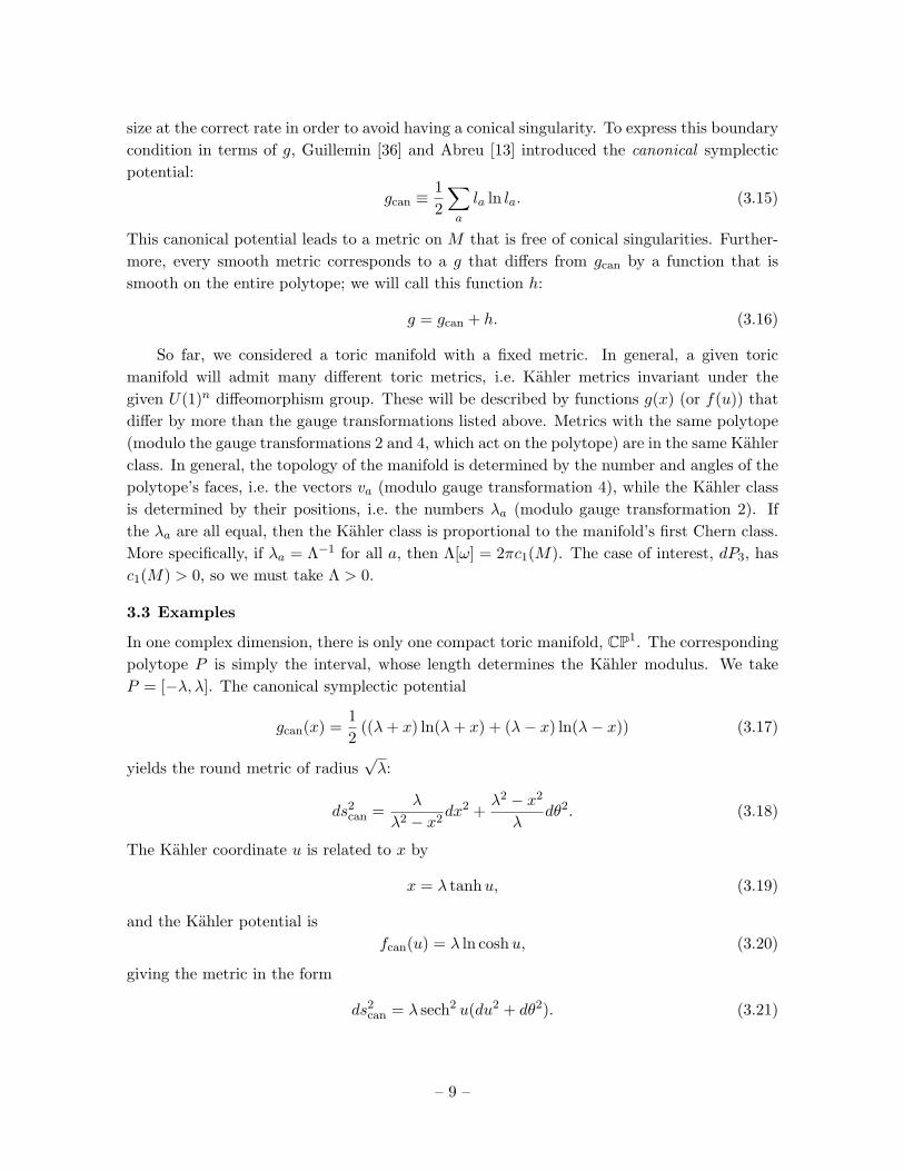
size at the correct rate in order to avoid having a conical singularity. To express this boundarycondition in terms of g, Guillemin [36] and Abreu [13] introduced the canonical symplecticpotential:
gcan ≡12
∑a
la ln la. (3.15)
This canonical potential leads to a metric on M that is free of conical singularities. Further-more, every smooth metric corresponds to a g that differs from gcan by a function that issmooth on the entire polytope; we will call this function h:
g = gcan + h. (3.16)
So far, we considered a toric manifold with a fixed metric. In general, a given toricmanifold will admit many different toric metrics, i.e. Kahler metrics invariant under thegiven U(1)n diffeomorphism group. These will be described by functions g(x) (or f(u)) thatdiffer by more than the gauge transformations listed above. Metrics with the same polytope(modulo the gauge transformations 2 and 4, which act on the polytope) are in the same Kahlerclass. In general, the topology of the manifold is determined by the number and angles of thepolytope’s faces, i.e. the vectors va (modulo gauge transformation 4), while the Kahler classis determined by their positions, i.e. the numbers λa (modulo gauge transformation 2). Ifthe λa are all equal, then the Kahler class is proportional to the manifold’s first Chern class.More specifically, if λa = Λ−1 for all a, then Λ[ω] = 2πc1(M). The case of interest, dP3, hasc1(M) > 0, so we must take Λ > 0.
3.3 Examples
In one complex dimension, there is only one compact toric manifold, CP1. The correspondingpolytope P is simply the interval, whose length determines the Kahler modulus. We takeP = [−λ, λ]. The canonical symplectic potential
gcan(x) =12
((λ+ x) ln(λ+ x) + (λ− x) ln(λ− x)) (3.17)
yields the round metric of radius√λ:
ds2can =λ
λ2 − x2dx2 +
λ2 − x2
λdθ2. (3.18)
The Kahler coordinate u is related to x by
x = λ tanhu, (3.19)
and the Kahler potential isfcan(u) = λ ln coshu, (3.20)
giving the metric in the form
ds2can = λ sech2 u(du2 + dθ2). (3.21)
– 9 –

Figure 1: The polytopes for the five compact toric manifolds with positive first Chern class: fromleft to right, CP1×CP1, CP2, dP1, dP2, dP3. Each polytope is drawn such that the λa for all its facesare equal, corresponding to the Kahler class being proportional to the first Chern class.
There are five compact toric surfaces with positive first Chern class (i.e. toric Fano sur-faces); their polytopes are shown in Fig. 1. CP1×CP1 has two moduli, the sizes of the two CP1
factors; when these are equal the canonical metric is Einstein. CP2 has only a size modulus,and again the canonical metric is Einstein, as shown in Appendix A. The del Pezzo surfacesdP1, dP2, and dP3 have two, three, and four moduli respectively. Their canonical metricsare never Einstein. Indeed, dP1 and dP2 do not admit Kahler-Einstein metrics at all [32],essentially because their Lie algebra of holomorphic one-forms is not reductive. The case ofdP3 is special. On the one hand, it is known to admit a toric Kahler-Einstein metric [6]. Onthe other hand, that metric is not the canonical one; indeed it is not known in closed form— hence the necessity of computing it numerically. dP3 is discussed in more detail in Section3.8 below.
3.4 The Monge-Ampere equation
As usual for a Kahler manifold, the Ricci curvature tensor Ri can be written in complexcoordinates z in a simple way, namely
Ri = − ∂2
∂zi∂zjln det gkl . (3.22)
Recall that there is a two-form R = iRidzi ∧ dzj associated with Ri where the class [R] =
2πc1(M). We are interested in Kahler-Einstein metrics on M , that is metrics which satisfythe following relation
Ri = Λgi (3.23)
for some fixed Λ. As explained above, this implies that λa = Λ−1 for all a. The sign of Λ isnot arbitrary but is fixed by the first Chern class of M , which we are now assuming to bepositive.
Given (3.22), we may integrate (3.23) twice, yielding
ln detFij = −2Λf + γ · u− c (3.24)
where γ and c are integration constants. In symplectic coordinates, this becomes
ln detGij = −2Λg +∂g
∂x· (2Λx− γ) + c . (3.25)
– 10 –

Both (3.24) and (3.25) are examples of Monge-Ampere type equations, which must be solvedwith the boundary conditions discussed in Section 3.2 above. The values of the constants γand c in these equations are arbitrary; given a solution with one set of values, a solution withany other set can be obtained using gauge transformations (1) and (2). However, as discussedabove, gauge transformation (2) acts on the polytope P by a translation. Therefore, if we fixthe position of P , there will be a unique γ such that (3.25) admits a solution.
Since the boundary conditions are non-standard, it is worth exploring them in moredetail. Again, we work in the symplectic coordinate system. Recall that the condition for asmooth metric was that h(x), defined by
g = gcan + h, (3.26)
be smooth on P , including on its boundary. We can re-write (3.25) in terms of h as follows:
ln det(δij +Gikcan
∂2h
∂xk∂xj
)= −2Λh+
∂h
∂x· (2Λx− γ)− ρcan + c , (3.27)
whereρcan ≡ ln detGcan
ij + 2Λgcan −∂gcan∂x
· (2Λx− γ). (3.28)
Normally, for a second-order PDE, we would expect to have to impose, for example, Dirichletor Neumann boundary conditions in order to obtain a unique solution. However, in the case of(3.25), the coefficient of the normal second derivative goes to zero (linearly) on the boundary(near the face a of the polytope, Gikcanv
ka ∼ la). Therefore, under the assumption that h and
its derivatives remain finite on the boundary, the equation itself imposes a certain (mixedDirichlet-Neumann) boundary condition. If we were to try to impose an extra one, we wouldfail to find a solution. This is illustrated by the case of CP1. Setting Λ = λ−1, we haveρcan = 0, so that (3.27) becomes
ln(
1 +λ2 − x2
λh′′
)=
2λ
(−h+ xh′) + c; (3.29)
we see that the coefficient of h′′ vanishes on the polytope boundary.For future reference we record here the formulas for the Ricci and Riemann tensors in
symplectic coordinates. Their non-zero components are
Rxixj = Rθiθj =12
(∂2
∂xi∂xj−Gkl
∂Gij∂xk
∂
∂xl
)ln detGij (3.30)
Rxixjxkxl= Rxixj
θkθl = Rθiθjxkxl
= Rθiθjθkθl =12GmnGml[iGj]nk (3.31)
Rθixjθkxl
= −Rxiθjθk
xl= −Rθi
xjxk
θl = Rxiθjxk
θl
=12
(Gijkl −GmnGijmGkln −GmnGml(iGj)nk
), (3.32)
where we’ve definedGijk ≡
∂Gjk∂xi
, Gijkl ≡∂Gjkl∂xi
. (3.33)
– 11 –

3.5 Volumes
Here follows a short discussion about volumes useful for understanding the relation betweenλa and Λ above.
We know that the volume of a complex surface M is
Vol(M) =12
∫Mω2 , (3.34)
while the volume of a curve C isVol(C) =
∫Cω . (3.35)
From the Kahler-Einstein condition (3.23), (3.4), and the fact that the class of the Ricci formis related to the first Chern class, [R] = 2πc1(M), it follows that [ω] = 2πc1(M)/Λ and that
Vol(M) =2π2
Λ2c1(M)2 . (3.36)
For CP2 blown up at k points, c21 = 9− k. Meanwhile, for our curve,
Vol(C) =2πΛc1(M) · C . (3.37)
In symplectic coordinates, it is easy to compute these volumes. From (3.8) or (3.10),the volume (3.34) reduces to 4π2 times the area of P . Setting Λ = 1 corresponds to settingthe λa = 1. For curves, the computation is similarly easy. For example, some simple torusinvariant curves correspond to edges of P , and the volume computation reduces to measuringthe length of an edge of P .
3.6 The Laplacian
The Laplacian acting on a scalar function ψ is,
4ψ =1√
det gαβ∂µ
[√det gαβ gµν∂νψ
]. (3.38)
In symplectic coordinates, the determinant of the metric√
det gαβ = 1. We consider afunction ψ invariant under the torus action, implying no dependence on the two angularcoordinates so that ψ = ψ(x1, x2). Thus, the Laplacian can be written in a simpler fashion:
4ψ =∂
∂xi
(Gij
∂ψ
∂xj
). (3.39)
The Laplacian thus depends on a third derivative of g. However since we are interested inEinstein metrics, we may take (3.25), differentiate it, and use it to eliminate this derivative.One then finds the form
4Eψ = GijE∂2ψ
∂xi∂xj− 2Λxi
∂ψ
∂xi. (3.40)
From this equation one deduces the interesting fact that the symplectic coordinates are eigen-functions of−4E with eigenvalue 2Λ — the symplectic coordinates are close to being harmoniccoordinates.
– 12 –

3.7 Harmonic (1, 1)-forms
A compact toric variety M of dimension n defined by a fan {va} of m rays has Betti numberb2 = m− n [37]. Moreover, dP3 has no holomorphic (nor antiholomorphic) 2-forms and thusmust have m − n harmonic (1,1)-forms. These (1,1)-forms are in one-to-one correspondencewith torus invariant Weil divisors Da modulo linear equivalence. The equivalence relationsare ∑
a
viaDa ∼ 0 . (3.41)
From their connection with the divisors Da, perhaps it is not surprising that these (1,1)-forms θa can be constructed from functions µa which have a singularity of the form ln(va ·x+1)along the boundaries of the polytope [13]. Moreover, they should satisfy Maxwell’s equations,
dθ = 0 and d ? θ = 0 . (3.42)
The first equation dθ = 0 is immediate from the local description of θi as ∂i∂µ. The otherequation is
0 = Diθi = gkiDkθi . (3.43)
Using the Bianchi identity, we find then
0 = gkiDθik = ∂
(gikθik
), (3.44)
orgikθik = constant . (3.45)
Now this last equation is rather interesting. The left hand side is the Laplacian operatoracting on µ. In symplectic coordinates, the left hand side can be rewritten to yield
∂
∂xi
(Gij
∂µ
∂xj
)= constant . (3.46)
Using the Kahler-Einstein condition, the left hand side becomes (3.40).The constant is easy to establish. We have that
Vol(M)giθi =∫Mθ ∧ ?ω . (3.47)
The Kahler form is self-dual under the Hodge star, ?ω = ω. Conventionally, we may write[θ] = 2πc1(D), assuming θ is the curvature of a line bundle O(D). Using finally that [ω] =2πc1(M) (for Λ = 1), we find that
giθi = 2D ·KK2
, (3.48)
where K is the canonical class of M . This constant is often referred to as the slope of O(D).
– 13 –

3.8 More on dP3
For dP3, the toric fan is described by the six rays spanned by
v1 = (1, 0) ; v2 = (1, 1) ; v3 = (0, 1) ; (3.49)
v4 = (−1, 0) ; v5 = (−1,−1) ; v6 = (0,−1) .
This fan leads to a dual polytope P which is a hexagon. As discussed above, when all sixλa are equal, the Kahler class is proportional to the first Chern class; we will choose λa = 1.In this case the polytope has a dihedral symmetry group D6, generated by the following Z2
reflection and Z6 rotation:
R1 =
[0 11 0
], R2 =
[1 1−1 0
]. (3.50)
This discrete symmetry will be shared by the Kahler-Einstein metric on dP3, and will thereforeplay an important role in our computations. Note that the element R3
2 acts as x→ −x, whichsets γ = 0 in (3.24) and (3.25). Note also that the D6 acts naturally on the group of Cartierdivisors on dP3 (and hence on the harmonic (1,1)-forms), as can easily be seen by thinkingof the set of va as divisors on the manifold.
The hexagon P has a natural interpretation as the intersection of the polytope for asymmetric unit (CP1)3, which is a cube with coordinates x1, x2, x3 satisfying |xi| ≤ 1, withthe plane x1 + x2 + x3 = 0. The intersection defines a natural embedding of dP3 into (CP1)3.Furthermore, the canonical metric on dP3 is simply the one induced from the Fubini-Studymetric on (CP1)3.
While the action of the symmetries in symplectic coordinates is geometrically clear, wewant to make explicit their description in complex coordinates. Note that the action of R2
on the complex coordinates ui is given by the inverse transpose of R2 since u = ∂g/∂x. ThusR2 acts as (u1, u2) 7→ (u2, u2 − u1). Similarly, R1 which is its own inverse transpose, actsby (u1, u2) 7→ (u2, u1). More explicitly, the relation between the complex and symplecticcoordinates for the canonical potentials is given by
X2 = e2u1 =1 + x1
1− x1
1 + x1 + x2
1− x1 − x2, (3.51)
Y 2 = e2u2 =1 + x2
1− x2
1 + x1 + x2
1− x1 − x2.
To invert these relations involves solving a cubic equation in one of the xi.There are six affine coordinate patches associated to the cones formed by pairs of neigh-
boring rays va. We denote the cone formed by the ray va and va+1 to be σa and the coordinate
– 14 –

system on σa by (ξa, ηa). The complex coordinates on the patches a = 1, . . . , 6 are
σ1 : (ξ1, η1) = (Y,XY −1)σ2 : (ξ2, η2) = (X−1Y,X)σ3 : (ξ3, η3) = (X−1, Y )σ4 : (ξ4, η4) = (Y −1, X−1Y )σ5 : (ξ5, η5) = (XY −1, X−1)σ6 : (ξ6, η6) = (X,Y −1)
(3.52)
Note that ηa = 1/ξa+1, and that when ξa = ηa+1, then ξa+1 = ηa. Because of these relations,we can consider an atlas on dP3 where for each σa, we restrict ξa ≤ 1 and ηa ≤ 1. These sixpolydisks Pa tile dP3.
In the symplectic coordinate system (x1, x2), our atlas divides the hexagon up into sixpieces. The boundaries are given by the conditions eu1 = 1, eu2 = 1, and eu1−u2 = 1 or insymplectic coordinates, the three lines 2x1 + x2 = 0, x1 + 2x2 = 0, and x1 − x2 = 0.
The action of D6 maps one Pa into another. For example in patch 3 since X and Y are theexponentials of u1 and u2, R2 acts on our coordinates by sending (X−1, Y ) → (Y −1, X−1Y ),mapping patch 3 into patch 4.
-1 -0.5
-1
0.5
Figure 2: The polytope P for dP3. The dashed lines correspond to the edges of the unit polydisks:2x1 + x2 = 0, x1 + 2x2 = 0, and x1 = x2. The red curved lines correspond to setting ξi and ηi equalto two instead of one in the appropriate coordinate systems.
4. Ricci flow
In this section we consider the flow, on the space of Kahler metrics on M , defined by (1.1):
∂gµν∂t
= −2Rµν + 2gµν , (4.1)
– 15 –

where we have set Λ = 1. Note that, since the Ricci form is a closed two-form, a Kahlermetric remains Kahler along the flow. Furthermore, if [ω] = [R] for the initial metric, thenthe flow will stay within that Kahler class. If the flow converges, the limiting metric willclearly be Einstein. A recent result of Tian and Zhu [14] implies that, on dP3, starting fromany initial Kahler metric obeying [ω] = [R], the flow will indeed converge to the Kahler-Einstein metric. Numerical simulation of the flow can therefore be used as an algorithm forfinding the Kahler-Einstein metric.
Thanks to the toric symmetry, (4.1) can be written as a parabolic partial differentialequation for a single function in 2 space and 1 time dimensions, and therefore represents asimple problem in numerical analysis. Specifically, according to (3.22), we can write (4.1) interms of the Kahler potential f(u):
∂f
∂t= ln detFij + 2f + c. (4.2)
Here c, which is independent of u but may depend on t, can be chosen arbitrarily. In particular,the zero mode of f (which is pure gauge) is clearly unstable according to (4.2), and c is usefulfor controlling that instability. In principle we could also add a term γ · u to the right-handside. As explained in Section 3.8, however, due to the symmetry of the polytope for dP3,we know that γ = 0 in the solution to the Monge-Ampere Eq. (3.24). In the symplecticcoordinates, (4.2) takes the form
∂g
∂t= ln detGij + 2
(−x · ∂g
∂x+ g
)− c. (4.3)
Note that, because the Kahler potential is t-dependent, the mapping relating u to x is as well.To derive (4.3), we used the fact that, since f and g are related by a Legendre transform,∂g/∂t|x = −∂f/∂t|u. Note also that (4.3) does not quite describe Ricci flow in the symplecticcoordinate system; rather it describes Ricci flow supplemented with a t-dependent diffeomor-phism (described by the flow equation ∂gµν/∂t = −2Rµν +2gµν +2∇(µξν)). Under pure Ricciflow, symplectic coordinates do not stay symplectic, since the Ricci tensor (3.30) is not theHessian of a function, hence the necessity of supplementing the flow with a diffeomorphism.
The two flows (4.2) and (4.3) were simulated by two independent computer programs,which yielded consistent results. In both cases we represented the (Kahler or symplectic)potential using standard real space finite differencing, and therefore obtain the resultingapproximation to the geometry in the form of the potential at an array of points. (In thenext section we discuss how to present this information more compactly using polynomialapproximations.) We relegate technical details of these implementations to Appendix B.When using finite difference methods it is important to show that one obtains a suitableconvergence to a continuum limit upon refinement of the discrete equations, and we presenttests that confirm this, and estimate errors in the same appendix.
– 16 –

4.1 Complex coordinates
We now discuss in more detail the implementation of Ricci flow using complex coordinates.Our canonical Kahler potential fcan is defined in P ◦, the interior of the hexagon. To workon our atlas (3.52), we use Kahler transformations to modify the Kahler potential so that fis smooth on each coordinate patch, including the two relevant edges of the hexagon. ThisKahler transformation must also respect the U(1) isometries so must only depend on theui. The only such Kahler transformations are affine linear combinations of the ui. (For afunction h(u1+iθ1, u2+iθ2) depending only on the ui, the condition on Kahler transformations∂∂h ≡ 0 reduces to ∂2h
∂ui∂uj≡ 0.) In the interior of the hexagon, we can thus modify f without
modifying the metric by adding a linear combination of u1 and u2. In symplectic coordinates
u · κ =12
6∑a=1
va · κ ln(va · x+ 1)
where κ ∈ R2.We find that for any Kahler potential f , regardless of coordinate patch,
detFij = ξ2η2
[(1ξ
∂f
∂ξ+∂2f
∂ξ2
) (1η
∂f
∂η+∂2f
∂η2
)−
(∂2f
∂ξ∂η
)2]. (4.4)
We can rewrite (4.2), yielding
∂f
∂t= ln
[(1ξ
∂f
∂ξ+∂2f
∂ξ2
) (1η
∂f
∂η+∂2f
∂η2
)−
(∂2f
∂ξ∂η
)2]
+ 2(f + ln ξ + ln η) + c . (4.5)
This shift of f by logarithms is a Kahler transformation. In each coordinate patch, we canwrite ln ξa + ln ηa = u · κa where κ1 = (1, 0), κ2 = (0, 1), κ3 = (−1, 1), κ4 = (−1, 0),κ5 = (0,−1), and κ6 = (1,−1). Moreover, for these choices of κa, fa = f + u · κa is wellbehaved everywhere inside Pa including the edges.
We simulate Ricci flow using a Kahler-Einstein potential fa defined on a neighborhoodUa of Pa, Ua = {(ξa, ηa) : ξa, ηa < L,L > 1} which satisfies (4.5). As an initial condition,we take fa(t = 0) = fcan + ln ξa + ln ηa. Given two patches, a and b, then for a point in theoverlap, p ∈ Ua ∩ Ub,
fb(p) = fa(p) + u · (κb − κa) . (4.6)
These Kahler transformations are consistent with the canonical potential and thus fix thesame Kahler class. There is then an element R ∈ D6 such that R(Pb) = Pa which relates faand fb. In particular, if p in is in Ub and Rp is in Ua:
fb(p) = fa(Rp) . (4.7)
Thus, with these quasiperiodic boundary conditions along the interior edges ξa = L andηa = L, we can determine f by working solely on the patch Ua.
– 17 –
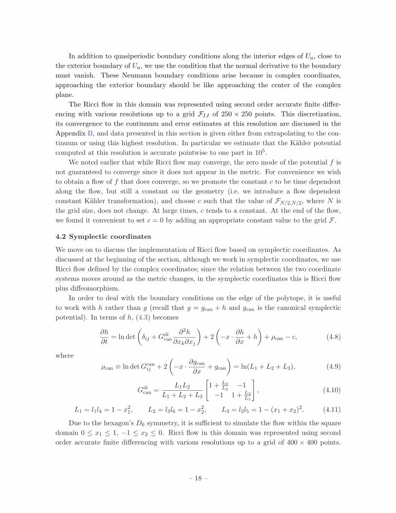
In addition to quasiperiodic boundary conditions along the interior edges of Ua, close tothe exterior boundary of Ua, we use the condition that the normal derivative to the boundarymust vanish. These Neumann boundary conditions arise because in complex coordinates,approaching the exterior boundary should be like approaching the center of the complexplane.
The Ricci flow in this domain was represented using second order accurate finite differ-encing with various resolutions up to a grid FIJ of 250 × 250 points. This discretization,its convergence to the continuum and error estimates at this resolution are discussed in theAppendix B, and data presented in this section is given either from extrapolating to the con-tinuum or using this highest resolution. In particular we estimate that the Kahler potentialcomputed at this resolution is accurate pointwise to one part in 105.
We noted earlier that while Ricci flow may converge, the zero mode of the potential f isnot guaranteed to converge since it does not appear in the metric. For convenience we wishto obtain a flow of f that does converge, so we promote the constant c to be time dependentalong the flow, but still a constant on the geometry (i.e. we introduce a flow dependentconstant Kahler transformation), and choose c such that the value of FN/2,N/2, where N isthe grid size, does not change. At large times, c tends to a constant. At the end of the flow,we found it convenient to set c = 0 by adding an appropriate constant value to the grid F .
4.2 Symplectic coordinates
We move on to discuss the implementation of Ricci flow based on symplectic coordinates. Asdiscussed at the beginning of the section, although we work in symplectic coordinates, we useRicci flow defined by the complex coordinates; since the relation between the two coordinatesystems moves around as the metric changes, in the symplectic coordinates this is Ricci flowplus diffeomorphism.
In order to deal with the boundary conditions on the edge of the polytope, it is usefulto work with h rather than g (recall that g = gcan + h and gcan is the canonical symplecticpotential). In terms of h, (4.3) becomes
∂h
∂t= ln det
(δij +Gikcan
∂2h
∂xk∂xj
)+ 2
(−x · ∂h
∂x+ h
)+ ρcan − c, (4.8)
where
ρcan ≡ ln detGcanij + 2
(−x · ∂gcan
∂x+ gcan
)= ln(L1 + L2 + L3), (4.9)
Gikcan =L1L2
L1 + L2 + L3
[1 + L3
L2−1
−1 1 + L3L1
], (4.10)
L1 = l1l4 = 1− x21, L2 = l3l6 = 1− x2
2, L3 = l2l5 = 1− (x1 + x2)2. (4.11)
Due to the hexagon’s D6 symmetry, it is sufficient to simulate the flow within the squaredomain 0 ≤ x1 ≤ 1, −1 ≤ x2 ≤ 0. Ricci flow in this domain was represented using secondorder accurate finite differencing with various resolutions up to a grid of 400 × 400 points.
– 18 –

The differencing, continuum convergence and errors at this resolution are discussed in theAppendix B with data presented in this section given either from extrapolating to the con-tinuum or using this highest resolution. In that appendix we estimate that the symplecticpotential computed at this resolution is accurate to one part in 106 at a given point.
As for the complex coordinates, the zero mode of the symplectic potential is pure gaugeand does not converge. The constant c was promoted to depend on flow time and chosen tokeep h(0, 0, t) = 0.
4.3 Results
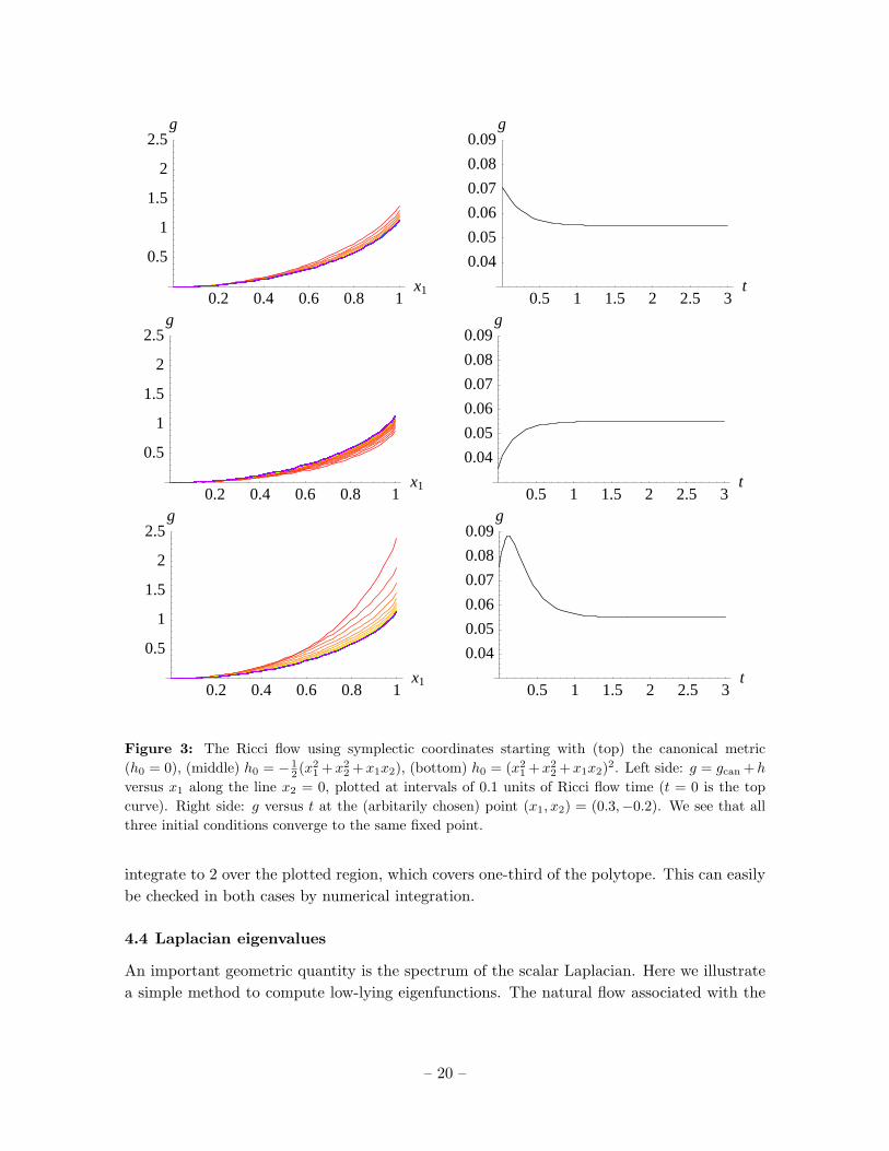
As predicted by the Tian-Zhu theorem, the metric converges smoothly and uneventfully tothe Kahler-Einstein one. In the symplectic implementation, the Ricci flow was simulatedstarting with a variety of initial functions h0(x) = h(x, t = 0) (always corresponding, ofcourse, to positive-definite initial metrics). Three examples are shown in Fig. 3. For everyinitial function investigated, the flow converged to the same fixed point hE(x) = h(x, t = ∞),which necessarily represents the Kahler-Einstein metric. The exponential approach to thefixed point is controlled by the scalar Laplacian; this will be discussed in detail in the nextsubsection.
The final complex and symplectic potentials found by the independent implementationsare plotted in Figs. 4 and 5, along with the respective canonical potentials. The results areplotted in the fundamental domain actually simulated, and one should use the D6 symmetryto picture the potentials extended over the whole domain. To compare the Kahler potentialfE(u) computed in complex coordinates with the symplectic potential gE(x) computed insymplectic coordinates, we numerically performed a Legendre transform to obtain a Kahlerpotential f ′E(u) from gE(x). Plotting f ′E − fE in Fig. 6, it can be seen that they differ by lessthan 5 × 10⁻⁶. (In fact the agreement may be slightly better as there is likely some errorintroduced in doing the numerical Legendre transform.) Thus our results appear to agree toaround the same order that we believe they are accurate.
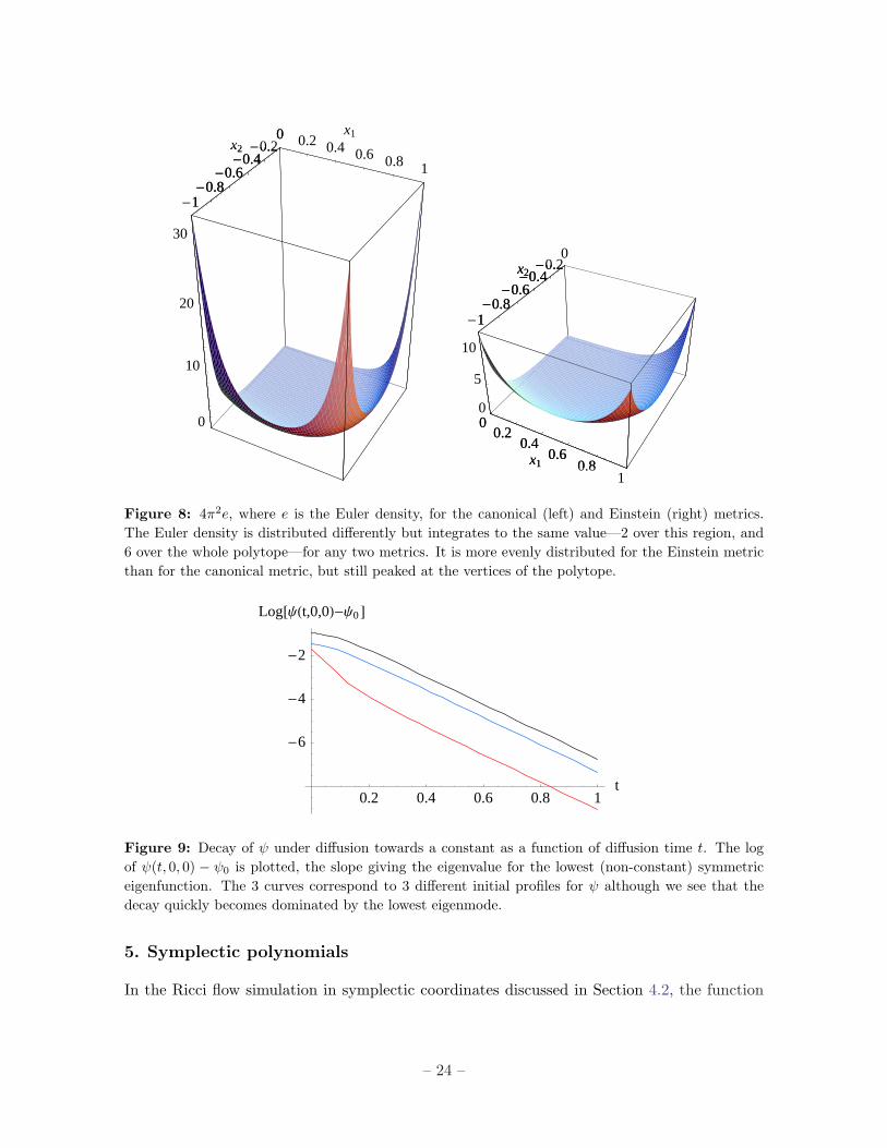
In order to get some feeling for the form of the Kahler-Einstein metric, and how itcompares to the canonical one, it is helpful to plot some curvature invariants. Of course, anyinvariant depending solely on the Ricci tensor, such as the Ricci scalar, will be trivial, so weneed to go to invariants constructed from the Riemann tensor. (Expressions for the Riemanntensor are given in Section 3.4 above.) For example, the sectional curvature of the x1-x2 plane(at fixed θi), which is Rx1x2x1x2/det(Gij), is plotted for the canonical and Einstein metricsin Fig. 7. Also of interest is the Euler density
e =1
32π2
(R2 − 4RµνRµν +RµνρλR
µνρλ), (4.12)
which integrates to the Euler character of the manifold, which is 6 for dP3. The first twoterms inside the parentheses cancel in the case of an Einstein metric. Fig. 8 shows 4π2e forthe canonical and Einstein metrics. The factor of 4π2 takes account of the coordinate volumeof the fiber. Recalling that
√g = 1 in symplectic coordinates, the plotted quantity should
– 19 –
0.2 0.4 0.6 0.8 1x1
0.5
1
1.5
2
2.5g
0.5 1 1.5 2 2.5 3t
0.04
0.05
0.06
0.07
0.08
0.09g
0.2 0.4 0.6 0.8 1x1
0.5
1
1.5
2
2.5g
0.5 1 1.5 2 2.5 3t
0.04
0.05
0.06
0.07
0.08
0.09g
0.2 0.4 0.6 0.8 1x1
0.5
1
1.5
2
2.5g
0.5 1 1.5 2 2.5 3t
0.04
0.05
0.06
0.07
0.08
0.09g
Figure 3: The Ricci flow using symplectic coordinates starting with (top) the canonical metric(h0 = 0), (middle) h0 = − 1
2 (x21 +x2
2 +x1x2), (bottom) h0 = (x21 +x2
2 +x1x2)2. Left side: g = gcan +h
versus x1 along the line x2 = 0, plotted at intervals of 0.1 units of Ricci flow time (t = 0 is the topcurve). Right side: g versus t at the (arbitarily chosen) point (x1, x2) = (0.3,−0.2). We see that allthree initial conditions converge to the same fixed point.
integrate to 2 over the plotted region, which covers one-third of the polytope. This can easilybe checked in both cases by numerical integration.
4.4 Laplacian eigenvalues
An important geometric quantity is the spectrum of the scalar Laplacian. Here we illustratea simple method to compute low-lying eigenfunctions. The natural flow associated with the
– 20 –

a)
00.2
0.40.6
0.81
Ξ
0
0.2
0.4
0.6
0.8
1
Η
-0.75-0.5-0.25
00.25
00.2
0.40.6
0.8Ξ
b)
00.2
0.40.6
0.81
Ξ
0
0.2
0.4
0.6
0.8
1
Η
-1
-0.5
0
00.2
0.40.6
0.8Ξ
c)
00.2
0.40.6
0.81
Ξ
0
0.2
0.4
0.6
0.8
1
Η
0.3
0.4
0.5
00.2
0.40.6
0.8Ξ
Figure 4: a) The Einstein Kahler potential fE as a function of ξ and η; b) the canonical potentialfcan(ξ, η); and c) fE(ξ, η)− fcan(ξ, η).
scalar Laplacian is diffusion, and the late time asymptotic behavior of the diffusion flowis dominated by the eigenfunction with lowest eigenvalue. Hence simulating diffusive flowon the dP3 geometry found, and extracting the asymptotics of this flow allows the lowesteigenfunction to be studied. We may classify the eigenfunctions under action of the D6 andU(1)2 isometries. Since the flow equation is invariant under these symmetries, if we startwith initial data that transforms in a particular representation, the function at any later timein the flow will remain in this representation. For simplicity we will focus on eigenfunctionswhich transform trivially, but obviously the method straightforwardly generalizes to computethe low-lying eigenfunctions in other sectors. As for the Ricci flow, the flow does not dependon second normal derivatives of ψ at the boundaries of the hexagon domain, and hence wedo not require boundary conditions for ψ there, except to require it to be smooth.
The lowest eigenfunction of −4E in the symmetry sector we study is ψ = constantwhich has zero eigenvalue. We are interested in the next lowest mode which has positiveeigenvalue and non-trivial eigenfunction, denoted ψ1(x) with eigenvalue λ1. Then we considerthe diffusion flow on our del Pezzo solution,
∂
∂tψ(t, x) = 4Eψ(t, x) (4.13)
and start with initial data for ψ that is symmetric and will hence remain symmetric. At latetimes, the flow will generically behave as,
ψ(t, x) = ψ0 + ψ1(x)e−λ1t +O(e−λ2t) (4.14)
where ψ0 is a constant, corresponding to the trivial zero eigenmode, and λ2 is the next lowesteigenvalue λ2 > λ1. Waiting long enough and subtracting out the trivial constant, the lateflow is given by ψ1, the eigenfunction we wish to compute.
In Fig. 9 we plot the log of ψ(t, 0, 0)− ψ0 as a function of the flow time t for 3 differentinitial data. Once the higher eigenmodes have decayed away, we clearly see the flows tend tothe same exponential behaviour. We estimate this eigenvalue by fitting the exponential decay
– 21 –

0
0.2
0.40.6
0.81
x1
-1-0.8
-0.6-0.4-0.20
x2
0
0.5
1
0.2
0.40.6
0.81
x1
-
-0.8-0.6
-0.4
0
0.2
0.40.6
0.81
x1
-1-0.8
-0.6-0.4-0.20
x2
0
0.25
0.5
0.75
1
0.2
0.40.6
0.81
x1
-
-0.8-0.6
-0.4
00.2
0.40.6
0.81
x1
-1
-0.8
-0.6
-0.4
-0.2
0
x2
-0.2
-0.1
0
00.2
0.40.6
0.8x1
Figure 5: Top left: The canonical symplectic potential gcan. Top right: The Einstein symplecticpotential gE = gcan + hE. Bottom: hE. These are plotted in the range 0 ≤ x1 ≤ 1, −1 ≤ x2 ≤ 0,which is one-third of the hexagon; the values on the rest of the hexagon are determined from these byits D6 symmetry.
as λ1 = 6.32. In Fig. 10 we plot the eigenfunction ψ1(x), normalized so that ψ1(0, 0) = 1.Note that, as expected, for different initial data we consistently obtain the same function.
This lowest eigenvalue and eigenfunction can also be obtained from the approach tothe fixed point of the Ricci flow. For concreteness let us work in symplectic coordinates;corresponding expressions will hold in complex coordinates. Expanding h about its fixed-point value,
h = hE + δh, (4.15)
the flow equation (4.8) becomes, to first order in δh,
∂δh
∂t= (4E + 2)δh− δc, (4.16)
– 22 –
0.20.4
0.60.8
1
Ξ0.2
0.4
0.6
0.8
1
Η
-4´10-6
-2´10-6
0
0.20.4
0.60.8Ξ
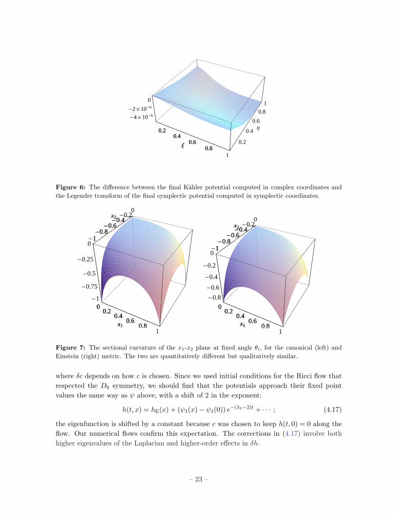
Figure 6: The difference between the final Kahler potential computed in complex coordinates andthe Legendre transform of the final symplectic potential computed in symplectic coordinates.
00.2
0.40.6
0.81
x1
-1-0.8-0.6-0.4-0.2
0x2
-1
-0.75
-0.5
-0.25
0
00.2
0.40.6
0.8x1
-1-0.8-0.6-0.4-0.2x2
00.2
0.40.6
0.81
x1
-1-0.8-0.6-0.4-0.2
0x2
-0.8
-0.6
-0.4
-0.2
0
00.2
0.40.6
0.8x1
-1-0.8-0.6-0.4-0.2x2
Figure 7: The sectional curvature of the x1-x2 plane at fixed angle θi, for the canonical (left) andEinstein (right) metric. The two are quantitatively different but qualitatively similar.
where δc depends on how c is chosen. Since we used initial conditions for the Ricci flow thatrespected the D6 symmetry, we should find that the potentials approach their fixed pointvalues the same way as ψ above, with a shift of 2 in the exponent:
h(t, x) = hE(x) + (ψ1(x)− ψ1(0)) e−(λ1−2)t + · · · ; (4.17)
the eigenfunction is shifted by a constant because c was chosen to keep h(t, 0) = 0 along theflow. Our numerical flows confirm this expectation. The corrections in (4.17) involve bothhigher eigenvalues of the Laplacian and higher-order effects in δh.
– 23 –
0 0.2 0.4 0.6 0.8 1
x1
-1-0.8-0.6-0.4-0.2
0x2
0
10
20
30
-1-0.8-0.6-0.4-0.2x2
00.2
0.40.6
0.81
x1
-1-0.8-0.6-0.4-0.2
0x2
0
5
10
00.2
0.40.6
0.8x1
-1-0.8-0.6-0.4-0.2x2
Figure 8: 4π2e, where e is the Euler density, for the canonical (left) and Einstein (right) metrics.The Euler density is distributed differently but integrates to the same value—2 over this region, and6 over the whole polytope—for any two metrics. It is more evenly distributed for the Einstein metricthan for the canonical metric, but still peaked at the vertices of the polytope.
0.2 0.4 0.6 0.8 1t
-6
-4
-2
Log@ΨHt,0,0L-Ψ0 D
Figure 9: Decay of ψ under diffusion towards a constant as a function of diffusion time t. The logof ψ(t, 0, 0) − ψ0 is plotted, the slope giving the eigenvalue for the lowest (non-constant) symmetriceigenfunction. The 3 curves correspond to 3 different initial profiles for ψ although we see that thedecay quickly becomes dominated by the lowest eigenmode.
5. Symplectic polynomials
In the Ricci flow simulation in symplectic coordinates discussed in Section 4.2, the function
– 24 –

00.2
0.4
0.6
0.8
1 -1
-0.8
-0.6
-0.4
-0.2
0
-1-0.5
00.51
00.2
0.4
0.6
0.8
Figure 10: The lowest eigenfunction of the scalar Laplacian which transforms trivially under the D6
and U(1)2 symmetries.
h(x) — which encodes the symplectic potential and therefore the metric — was representedby its values on a lattice of points in x1, x2. In this section we will discuss a different way torepresent the same function, namely as a polynomial in x1, x2. Since the solution hE to theMonge-Ampere equation is a smooth function, it can be represented to good accuracy witha vastly smaller amount of data in this way: a few polynomial coefficients as compared tovalues on thousands of lattice points. Furthermore, quite independent of the solutions foundin the previous section, the problem of finding an approximate solution to the Monge-Ampereequation can be expressed as an optimization problem for the polynomial coefficients; we willuse this fact to develop a third algorithm in the following section that is quite different incharacter from Ricci flow.
It is interesting to note that the metrics obtained from polynomial expressions for h(x)are the symplectic analogues of the so-called “algebraic” metrics on Calabi-Yau manifoldsthat have been used for numerical work by Donaldson [3] and Douglas et al. [4, 5]. Thealgebraic metrics, which are defined for a Calabi-Yau embedded in a projective space, have aKahler potential that differs from the induced Fubini-Study one by (the logarithm of) a finitelinear combination of a certain basis of functions, namely the pull-backs of the Laplacianeigenfunctions on the embedding projective space. This is a generalization of the usualstrategy of representing a function by expanding it in a basis of Laplacian eigenfunctions(such as Fourier modes); since the eigenfunctions on the Calabi-Yau depend on the metricthat one is trying to find, one instead uses the eigenfunctions on the embedding space, whichare known in closed form (and are indeed very simple). In our case, we consider the embeddingof dP3 in (CP1)3, which, as discussed in Section 3.8, is described in symplectic coordinates bythe equation x1 + x2 + x3 = 0 (where the xi are the symplectic coordinates on the respectiveCP1 factors). The first n eigenspaces of the Laplacian on (CP1)3 (with respect to the Fubini-
– 25 –

Study metric), restricted functions that are invariant under the U(1)3 isometry group, arespanned by the monomials in x1, x2, x3 up to order n. This is precisely the basis of functionswe use to expand the difference h between the symplectic potential g and the induced onegcan.
We now describe some fits to the numerical solutions of the last section in terms ofpolynomials up to sixth order in x1 and x2, and quantify how well those polynomials do insolving the Einstein equation. These small polynomials likely provide sufficiently accurateapproximations to the Einstein symplectic potential for most purposes, while at the sametime being more tractable than the full numerical data for analytic calculations.
We begin by noting that, since hE is invariant under the hexagon’s D6 symmetry group,it is sufficient to consider invariant polynomials. As shown in Appendix C, every invariantpolynomial can be expressed in terms of the two basic invariant polynomials,
U = x21 + x1x2 + x2
2 , V = x21x
22(x1 + x2)2 . (5.1)
We simply do a least-squares fit of the polynomial coefficients to the lattice values of hE
obtained in the Ricci flow in symplectic coordinates, that is, we minimize
α2 =1
VdP3
∫dP3
√g (hfit − hE)2 −
(1
VdP3
∫dP3
√g (hfit − hE)
)2
. (5.2)
(Any constant difference between hfit and hE is irrelevant). At successive orders in x we findthe following fits:
hfit α β
0 0.06 0.5−0.24U 10−3 0.1−0.2214U − 0.0215U2 10−4 0.03−0.22412U − 0.01450U2 − 0.00521U3 + 0.00734V 10−5 0.007
(5.3)
In each case we have written only the significant digits of the coefficients.3 Independently ofour numerical result hE, it is useful to know how far the metric corresponding to hfit deviatesfrom being Einstein. In Fig. 11, the pointwise rms deviation of the eigenvalues of the Riccitensor from 1,
D ≡√
14(Rµν − gµν)2, (5.4)
is plotted for these four functions. The global rms deviation from being Einstein, β, where
β2 =1
VdP3
∫dP3
√gD2, (5.5)
is also shown in the table above. As expected, each successive order gives a substantiallybetter approximation, and a metric that is substantially closer to being Einstein.
3These digits do not change between the run with 200 lattice points and the run with 400 lattice points
(except the last digit of each coefficient in the sixth-order approximation), and are therefore presumably equal
to their continuum values.
– 26 –

00.2
0.40.6
0.81
x1
-1
-0.8
-0.6
-0.4
-0.2
0
x2
0.51
1.52
00.2
0.40.6
0.8x1
00.2
0.40.6
0.8x1
-0.8
-0.6
-0.4
-0.2
0
x2
0.2
0.4
00.2
0.40.6
0.8x1
00.2
0.40.6
0.8x1
-0.8
-0.6
-0.4
-0.2
0
x2
0.05
0.1
0.15
00.2
0.40.6
0.8x1
00.2
0.40.6
0.8x1
-0.8
-0.6
-0.4
-0.2
0
x2
0.02
0.04
00.2
0.40.6
0.8x1
Figure 11: D ≡√
14 (Rµν − gµν)2 versus x1, x2 for the four polynomial functions listed in (5.3). The
deviation from being Einstein is most significant along the edges of the hexagon in the first two cases,and at the corners in the second two.
For eigenfunctions of the Laplacian, we may perform the same invariant polynomial fitsas we did for h; at quadratic order we find ψ1 ≈ 0.985− 2.37U .
We regard table 5.3 as a key result of this paper. The last line of the table provides in anextremely compact, analytic form, an approximation to the true symplectic potential on dP3.It deviates from the true potential pointwise by at most ∼ 0.1%, and satisfies the Einsteincondition well within the hexagon, giving at most a 10% error near the hexagon corners asmeasured by the pointwise rms deviation of the Ricci tensor eigenvalues, defined above.
6. Constrained optimization
In the previous section we used the results of Ricci flow to find a polynomial approximationto h(x), the smooth part of the Kahler-Einstein symplectic potential (recall that h ≡ g −
– 27 –

gcan). Here we instead search for a polynomial approximation to h using the Monge-Ampereequation directly. A simple approach would be to consider the space of polynomials of somegiven order, and minimize an error function built from the Monge-Ampere equation on thatspace. However, if one wishes to obtain high accuracies, one needs to go to high orders,and then this brute force approach rapidly becomes intractable due to the large numberof polynomial coefficients and the difficulty of searching in a high dimensional space. Wetherefore take advantage of the analytic properties of the Monge-Ampere equation to constrainthe polynomial coefficients, by requiring the polynomial to solve it order by order in xi. As wewill see, this leaves only a small number of undetermined parameters, dramatically simplifyingthe error function minimization. We now explain the details of the method.
We begin by noting that the exact solution hE(x) to the Monge-Ampere equation is ananalytic function of the xi, which can be seen in a couple of ways. As noted, the symplecticcoordinates are eigenfunctions of the Laplacian. Hence, in these coordinates the Ricci curva-ture operator has the same character as it does in harmonic cooordinates: it is actually anelliptic operator. Because the Einstein equations are analytic in the metric, they will haveanalytic solutions. Somewhat more directly, the Monge-Ampere equation we are solving iselliptic at the Kahler-Einstein potential and analytic, and so the solution will be analytic.
Before we constrain the polynomial approximation to h(x) using the Monge-Ampere equa-tion, we constrain it by imposing the hexagon’s D6 discrete symmetry group. As discussedin Section 5, any invariant polynomial in xi can be written in the form
h =∑i,j
ci,jUiV j , (6.1)
where U and V are given in Eq. (5.1). To eighteenth order in x1 and x2 we write the seriesas follows
h = A0 +A1U +A2U2 +A3U
3 +A4U4 +A5U
5 +A6U6 +A7U
7 +A8U8 +A9U
9 + . . .
+V (B0 +B1U +B2U2 +B3U
3 +B4U4 +B5U
5 +B6U6 + . . .)
+V 2 (C0 + C1U + C2U2 + C3U
3 + . . .) + V 3 (D0 + . . .) + . . . . (6.2)
Plugging this series into the Monge-Ampere equation (3.27) (with γ = 0 and Λ = 1),yields constraints on the ci,j that relate the ci,j with j > 0 to the ci,0. To make the expressionsa little simpler, we introduce a new constant α:
A0 = −12
ln 3− lnα . (6.3)
We worked out the relations up to order 18 in x1 and x2. The first relation is that A1 = −1±α.The numerical Ricci flow results are consistent only with the plus sign. The next few relationsare
A2 = −16
+α2
4, A3 = − 2
27− 2B0
27+
11α3
72; A4 = − 1
28− 5α
378− 25
189αB0 +
145α4
1152;
– 28 –
B1 =2514αB0 +
128
(−4 + 5α) ; B2 =8532α2B0 +
1192
(−32 + 51α2) .
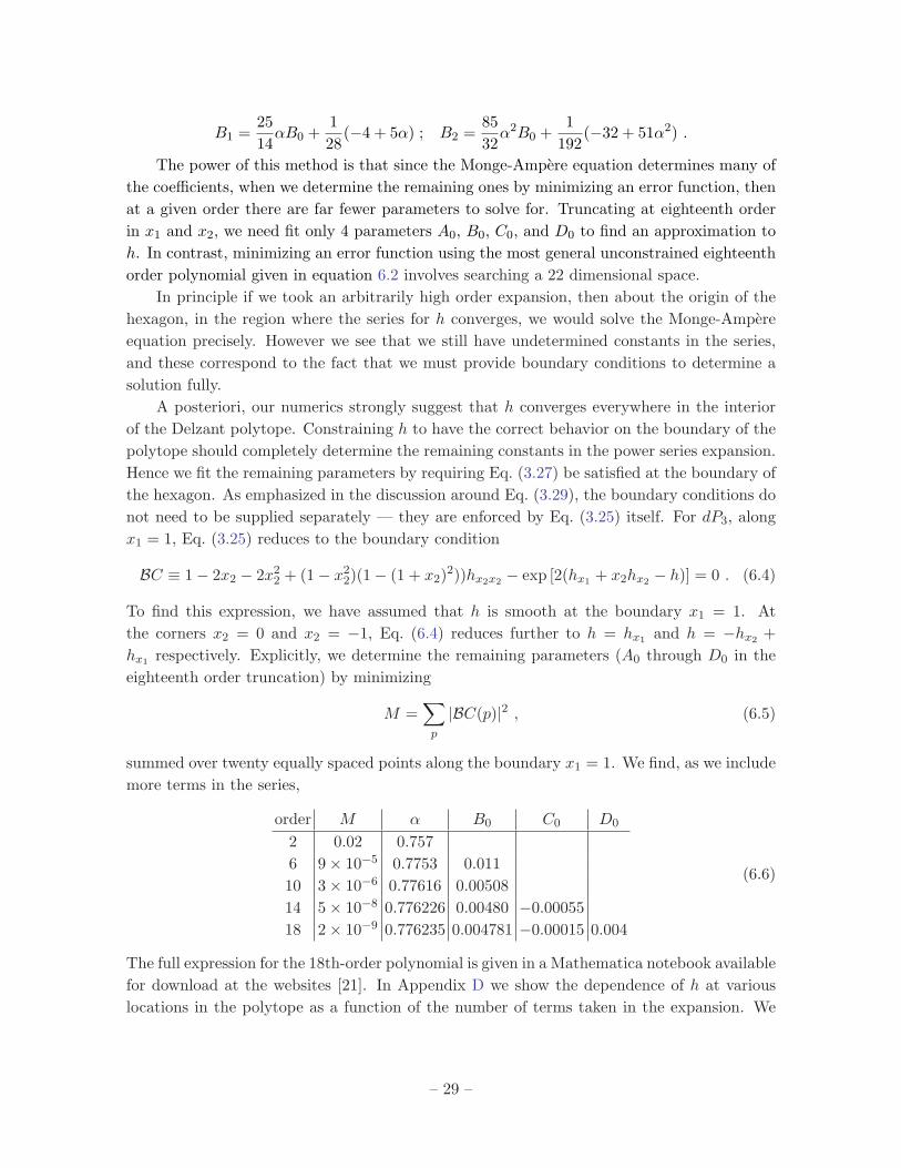
The power of this method is that since the Monge-Ampere equation determines many ofthe coefficients, when we determine the remaining ones by minimizing an error function, thenat a given order there are far fewer parameters to solve for. Truncating at eighteenth orderin x1 and x2, we need fit only 4 parameters A0, B0, C0, and D0 to find an approximation toh. In contrast, minimizing an error function using the most general unconstrained eighteenthorder polynomial given in equation 6.2 involves searching a 22 dimensional space.
In principle if we took an arbitrarily high order expansion, then about the origin of thehexagon, in the region where the series for h converges, we would solve the Monge-Ampereequation precisely. However we see that we still have undetermined constants in the series,and these correspond to the fact that we must provide boundary conditions to determine asolution fully.
A posteriori, our numerics strongly suggest that h converges everywhere in the interiorof the Delzant polytope. Constraining h to have the correct behavior on the boundary of thepolytope should completely determine the remaining constants in the power series expansion.Hence we fit the remaining parameters by requiring Eq. (3.27) be satisfied at the boundary ofthe hexagon. As emphasized in the discussion around Eq. (3.29), the boundary conditions donot need to be supplied separately — they are enforced by Eq. (3.25) itself. For dP3, alongx1 = 1, Eq. (3.25) reduces to the boundary condition
BC ≡ 1− 2x2 − 2x22 + (1− x2
2)(1− (1 + x2)2))hx2x2 − exp [2(hx1 + x2hx2 − h)] = 0 . (6.4)
To find this expression, we have assumed that h is smooth at the boundary x1 = 1. Atthe corners x2 = 0 and x2 = −1, Eq. (6.4) reduces further to h = hx1 and h = −hx2 +hx1 respectively. Explicitly, we determine the remaining parameters (A0 through D0 in theeighteenth order truncation) by minimizing
M =∑p
|BC(p)|2 , (6.5)
summed over twenty equally spaced points along the boundary x1 = 1. We find, as we includemore terms in the series,
order M α B0 C0 D0
2 0.02 0.7576 9× 10⁻⁵ 0.7753 0.01110 3× 10⁻⁶ 0.77616 0.0050814 5× 10⁻⁸ 0.776226 0.00480 −0.0005518 2× 10⁻⁹ 0.776235 0.004781 −0.00015 0.004
(6.6)
The full expression for the 18th-order polynomial is given in a Mathematica notebook availablefor download at the websites [21]. In Appendix D we show the dependence of h at variouslocations in the polytope as a function of the number of terms taken in the expansion. We
– 29 –
see that convergence for h is fast — apparently faster than polynomial — in the number ofterms, and in particular for everywhere tested within the hexagon, and also on its boundary,we see convergence. In particular we see no sign of poor behaviour near or on the boundariesof the hexagon. We also see that the values the series converges to are in excellent agreementwith the continuum extrapolated values of h found from the Ricci flow method and detailedin Appendix B. From these data we estimate that the potential given by the eighteenthorder expansion differs from the true solution by approximately one part in 106, and henceis comparable in this respect to the 400× 400 Ricci flow result.
The figure of merit M does not give a very good indication of the degree of accuracy ofour fit globally. To understand how well we are doing globally, we use the same local estimate
of error as in the previous section, D =√
14(Rµν − gµν)2. We find that the maximum value D
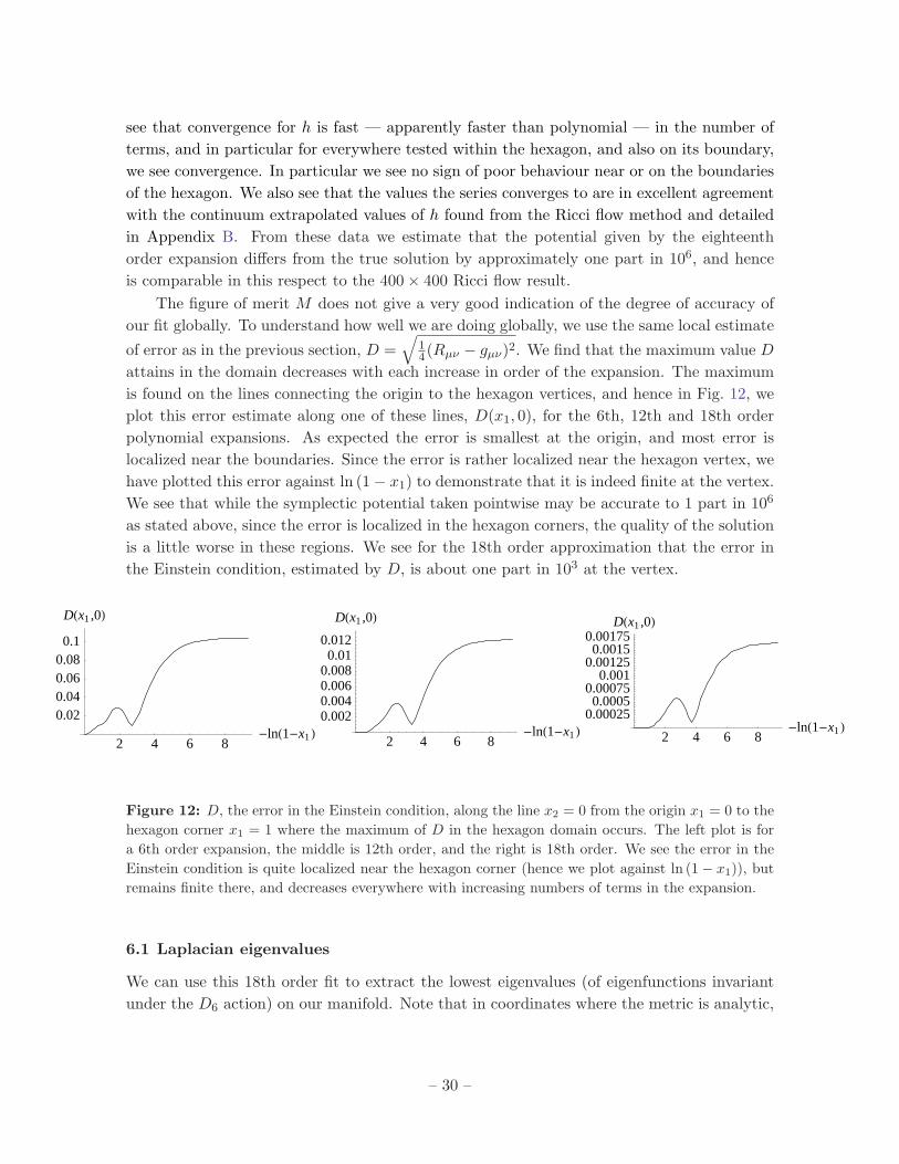
attains in the domain decreases with each increase in order of the expansion. The maximumis found on the lines connecting the origin to the hexagon vertices, and hence in Fig. 12, weplot this error estimate along one of these lines, D(x1, 0), for the 6th, 12th and 18th orderpolynomial expansions. As expected the error is smallest at the origin, and most error islocalized near the boundaries. Since the error is rather localized near the hexagon vertex, wehave plotted this error against ln (1− x1) to demonstrate that it is indeed finite at the vertex.We see that while the symplectic potential taken pointwise may be accurate to 1 part in 106
as stated above, since the error is localized in the hexagon corners, the quality of the solutionis a little worse in these regions. We see for the 18th order approximation that the error inthe Einstein condition, estimated by D, is about one part in 103 at the vertex.
2 4 6 8-lnH1-x1 L
0.020.040.060.08
0.1
DHx1 ,0L
2 4 6 8-lnH1-x1 L
0.0020.0040.0060.008
0.010.012
DHx1 ,0L
2 4 6 8-lnH1-x1 L
0.000250.0005
0.000750.001
0.001250.0015
0.00175DHx1 ,0L
Figure 12: D, the error in the Einstein condition, along the line x2 = 0 from the origin x1 = 0 to thehexagon corner x1 = 1 where the maximum of D in the hexagon domain occurs. The left plot is fora 6th order expansion, the middle is 12th order, and the right is 18th order. We see the error in theEinstein condition is quite localized near the hexagon corner (hence we plot against ln (1− x1)), butremains finite there, and decreases everywhere with increasing numbers of terms in the expansion.
6.1 Laplacian eigenvalues
We can use this 18th order fit to extract the lowest eigenvalues (of eigenfunctions invariantunder the D6 action) on our manifold. Note that in coordinates where the metric is analytic,
– 30 –

eigenfunctions of the Laplacian are analytic: elliptic equations with analytic coefficients haveanalytic solutions. Thus we can play a very similar game, expressing the eigenvectors as alocal power series near the origin of the hexagon in the U and V variables:
ψ(U, V ) =110
+X1U +X2U2 +X3U
3 + Y1V + . . . . (6.7)
We have chosen to normalize ψ(0, 0) = 0.1. We could in principle have used the differentialequation to constrain some of the Xi and Yi, but we did not, aiming for a fit whose errorsare more evenly distributed over the hexagon. We fit a hundred equally spaced points in asquare domain 0 < x1 < 0.9 and −0.9 < x2 < 0 and minimize
Mψ =∑p
|4ψ + λψ|2 , (6.8)
as a function of λ and the Xi and Y1. By searching for successive local minima of Mψ, wecan extract successively higher eigenvalues. We find
order Mψ X1 X2 X3 Y1 λ1
2 0.006 −0.239 6.274 0.002 −0.246 0.011 6.3256 3× 10⁻⁵ −0.245 0.006 0.006 −0.024 6.322
(6.9)
order Mψ X1 X2 X3 Y1 λ2
4 0.5 −0.69 0.79 17.46 0.008 −0.67 0.70 0.16 −1.28 17.2
(6.10)
For the lower eigenvalue 6.32, note that the ratio of the first two coefficients −2.39 is inreasonably good agreement with the corresponding ratio −2.37/0.985 = −2.41 determined inSection 5.
The choice to minimize Mψ in the domain 0 < |xi| < 0.9 was a compromise that requiressome justification. First, since (3.25) enforces its own boundary conditions, minimizing Mψ
close to the boundary x1 = 1 is enforcing the boundary condition to first order in x1 − 1.Second, the power series approximation for ψ experimentally does not appear to have goodconvergence properties near the boundary. Experimentally, the best values for the coefficientsof the truncated power series (in the sense of agreeing with the coefficients of the power seriesitself) are obtained by making a compromise between minimizing over a set of points thatextends to the boundary and minimizing over a set of points for which the power series hasgood convergence properties.
6.2 Harmonic (1,1)-forms
As noted in Section 3.7, harmonic (1, 1)-forms and eigenfunctions of the Laplacian must satisfya very similar equation. We end this section with a computation of the harmonic (1, 1)-form
– 31 –
θa. Unlike the eigenfunctions computed above, θa does not transform trivially under D6.Thus, we assume that µa has a more general expansion of the form
µa = ln(1 + va · x) +∑n,m
cnmxn1x
m2 , (6.11)
We use the same least squares approach as above, minimizing
Mθ =∑p
|4µa − const|2 . (6.12)
Because of the explicit x1 ↔ x2 symmetry, we start with a = 2 and set cnm = cmn. Fittingto sixth order in x1 and x2, we find
c10 = −0.2250c20 = 0.0638 c11 = 0.0311c30 = −0.0301 c21 = 0.0059c40 = 0.0126 c31 = 0.0005 c22 = −0.0073c50 = −0.0150 c41 = −0.0245 c32 = −0.0240c60 = 0.0088 c51 = 0.0223 c42 = 0.0281 c33 = 0.0196
(6.13)
The value of Mθ ∼ 10−4 at the minimum implies an average error of 10−3 at each of the 100points. Note the error gets much worse outside the fitting domain |xi| > 0.9. The philosophyin this section is similar to that in the discussion of eigenfunctions: we are attempting to findmore accurate values of the cij rather than attempting to minimize the global error.
The fit also yields F ijθij = 0.6672, consistent with our expectations. We know that
ω =12
6∑a=1
θa . (6.14)
Clearly F iFi = 2. By the dihedral symmetry group, the value of F iθi should be independentof a. We conclude that
(θa)iF i =23. (6.15)
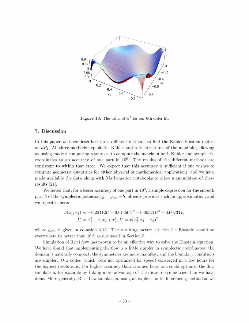
From θ2, we can reconstruct the other θa by applying the D6 group action. To test howgood our approximation to θ2 was, we computed Θ2 = ΘijΘij where Θij =
∑a(θa)ij using
our best fit for θ2. Since Θij should be 2Fij , Θ2 should be approximately eight. A plot of Θ2
is shown in Fig. 13.For the purposes of the KT solution described in the Introduction, we need a θ such that
θijFij = 0. From the preceding discussion, any linear combination of the form∑
a caθa suchthat
∑a ca = 0 will have this property. We also require that ?θ = −θ. In fact, the condition∑
a ca = 0 enforces anti-self-duality. The reason is that the Hodge star treated as a linearoperator acting on the space of harmonic (1,1)-forms has signature (+−−−). We know that?ω = ω; thus any (1,1)-form orthogonal to ω must be anti-self-dual. In general, the numericssuggest that for such a θ, θijθij will be a nontrivial function of both xi and thus that solvingfor h(p) requires solving a PDE in three real variables.
– 32 –
00.2
0.40.6
0.8x1 -0.8
-0.6
-0.4
-0.2
0
x2
7.967.98
88.028.04
00.2
0.40.6
0.8x1
Figure 13: The value of Θ2 for our 6th order fit.
7. Discussion
In this paper we have described three different methods to find the Kahler-Einstein metricon dP3. All three methods exploit the Kahler and toric structures of the manifold, allowingus, using modest computing resources, to compute the metric in both Kahler and symplecticcoordinates to an accuracy of one part in 106. The results of the different methods areconsistent to within that error. We expect that this accuracy is sufficient if one wishes tocompute geometric quantities for either physical or mathematical applications, and we havemade available the data along with Mathematica notebooks to allow manipulation of theseresults [21].
We noted that, for a lesser accuracy of one part in 103, a simple expression for the smoothpart h of the symplectic potential, g = gcan +h, already provides such an approximation, andwe repeat it here:
h(x1, x2) = −0.22412U − 0.01450U2 − 0.00521U3 + 0.00734V,
U = x21 + x1x2 + x2
2, V = x21x
22(x1 + x2)2 .
where gcan is given in equation 3.15. The resulting metric satisfies the Einstein conditioneverywhere to better than 10% as discussed in Section 5.
Simulation of Ricci flow has proven to be an effective way to solve the Einstein equation.We have found that implementing the flow is a little simpler in symplectic coordinates: thedomain is naturally compact; the symmetries are more manifest; and the boundary conditionsare simpler. Our codes (which were not optimized for speed) converged in a few hours forthe highest resolutions. For higher accuracy than attained here, one could optimize the flowsimulation, for example by taking more advantage of the discrete symmetries than we havedone. More generally, Ricci flow simulation, using an explicit finite differencing method as we
– 33 –

have done, can be thought of as a particular iterative scheme for solving the Monge-Ampereequation. If one is interested only in solving that equation, and not in accurately simulatingRicci flow, then this scheme could be modified to improve speed. For example, by replacingthe Jacobi-type updating method by a Gauss-Seidel method, one obtains a faster algorithm(experimentally, 50% faster in complex coordinates). To obtain a parametric improvement inspeed would likely require a non-local modification such as multi-grid.
The constrained optimization approach we have demonstrated uses the symplectic poly-nomials, reducing the size of the search space by solving the Monge-Ampere equation orderby order in xi, and has proven very powerful. It is as accurate as the Ricci flow results,but is quicker. One drawback is that the hexagon origin is singled out as the point wherethe solution is best, and the error in the solution becomes tightly localized at the cornersof the hexagon. Most computational time is invested in determining the constraints in theseries expansion, and this algebraic problem gets worse the more terms that are included inthe expansion. However, once one has this solution, the numerical minimization of the errorfunction is simple.
The two methods are complementary in the sense that for Ricci flow the time is spent innumerically computing the flow, whereas for the optimization the time is spent algebraicallycomputing the expansion of the potential. The principle advantage of Ricci flow is that themethod is very general, and while it benefits from the Kahler and toric structures it certainlyapplies to more general problems which do not possess them. It is not clear how widelyapplicable the constrained optimization approach is, as it likely works due to the specialproperties resulting from those mathematical structures. However, it would be interesting toinvestigate its application to other situations. It would also be interesting to compare theseapproaches, particularly the constrained optimization, with Donaldson’s method [3].
Acknowledgments
We would like to thank Ken Bube, Simon Donaldson, Richard Hamilton, Julien Keller, LiamMcAllister, Gang Tian, and Ursula Whitcher for discussion. C.H. would like to acknowledgethe support of the String Phenomenology Workshop at the KITP, UCSB and the PhysicsDepartment at the University of Texas, Austin where part of this work was done. C.D. issupported in part by a Royalty Research Fund Scholar Award from the Office of Research,University of Washington. M.H. is supported by the Stanford Institute for Theoretical Physicsand by NSF grant PHY 9870115. C.H. is supported in part by U.S. Department of Energyunder Grant No. DE-FG02-96ER40956 and by the National Science Foundation under GrantsNo. PHY99-07949 and No. PHY-0455649. J.K. is supported in part by a VIGRE graduatefellowship. T.W. is supported by a PPARC advanced fellowship and the Halliday award.
A. Canonical metric on CP2
Consider CP2 which has the fan, unique up to SL(2,Z) transformations, v1 = (1, 0), v2 =
– 34 –

(0, 1), and v3 = (−1,−1). We choose all the λa = 1 in gcan to assure that the class of theresulting Kahler form is proportional to the first Chern class,
gcan =12
[(1 + x1) ln(1 + x1) + (1 + x2) ln(1 + x2) + (1− x1 − x2) ln(1− x1 − x2)
]. (A.1)
From gcan, we can reconstruct the complex coordinates
1 + x1 =3e2u1
1 + e2u1 + e2u2; 1 + x2 =
3e2u2
1 + e2u1 + e2u2; (A.2)
1− x1 − x2 =3
1 + e2u1 + e2u2.
The canonical Kahler potential is then
fcan =32
ln(1 + e2u1 + e2u2)− 32
ln 3− u1 − u2 . (A.3)
The expression gcan satisfies (3.25) provided c = ln(4/3) and γ = 0. For CP2, the canoni-cal metric is the Fubini-Study metric. In terms of the traditional homogenous coordinates(X1, X2, X3) on CP2, the Kahler potential is traditionally written, with a different choice ofnormalization of the volume, in the patch X3 6= 0
ln(1 + |X1/X3|2 + |X2/X3|2) . (A.4)
Thus, we identify |X1/X3| = exp(u1) and |X2/X3| = exp(u2). The canonical metric is alwaysKahler-Einstein for Cartesian products of projective spaces [36].
B. Numerical Ricci flow implementation and error estimates
In this appendix we give technical details of our two finite difference implementations of Ricciflow, and also discuss the continuum convergence and estimate errors for the resolutions used.
B.1 Implementation in complex coordinates
We work on a square domain slightly bigger than a unit polydisk, 0 ≤ ξ ≤ L and 0 ≤ η ≤ L
(L > 1) where f is assumed to have Neumann boundary conditions along ξ = 0 and η = 0.Along the internal boundaries, ξ = L and η = L, we employ a kind of periodic boundarycondition enforced by the Z6 symmetry of the hexagon. We take
f(ξ, L) = f(1/L, ξL) + lnL , (B.1)
to map the boundary η = L for 0 ≤ ξ < 1/L back into our square domain. For 1/L < ξ < 1,we take a composition of the above map:
f(ξ, L) = f(1/(Lξ), ξ) + lnL2ξ . (B.2)
– 35 –
For the ξ = L boundary, we take the preceding rules with η and ξ switched. For the pointsalong the boundary with ξ > 1 or η > 1, we use the rule
f(ξ, η) = f(1/ξ, 1/η) + 2 ln ξ + 2 ln η . (B.3)
Note that as indicated in Section 4.1, due to the Z6 symmetry, for any point p = (ξ, η), withξ > 1 or η > 1, the value of f(p) should be related by a Kahler transformation to the valueof f at a point inside the unit polydisk.
Although we are only enforcing the Z6 symmetry along the boundary of our coordinatepatch, the symmetry will hold globally. First, our initial potential fcan respects the symmetry.Second, Ricci flow preserves the symmetry.
To discretize (4.2), we approximated f(ξ, η) by its values FIJ on anN×N grid with latticespacing ∆ = L/(N − 1) and used standard second order finite differencing for derivatives. Inevaluating the first order derivatives at the boundary, we took
1ξ
∂f
∂ξ
∣∣∣∣ξ=0
=∂2f
∂ξ2
∣∣∣∣ξ=0
and1η
∂f
∂η
∣∣∣∣η=0
=∂2f
∂η2
∣∣∣∣η=0
. (B.4)
To impose a discrete version of the boundary conditions, we added extra rows and columnsalong the grid. To impose Neumann boundary conditions, we imposed that F0,J = F2,J
and FI,0 = FI,2. To impose the periodic boundary conditions along the (I,N) and (N, J)boundaries, we mapped the the point (I,N + 1) or (N + 1, J) back inside the grid using thesymmetries and used a bicubic interpolation to compute a best value for f .
B.2 Implementation in symplectic coordinates
We represented h on a uniform square lattice in the variables x1, x2. Such a lattice hasseveral advantages, aside from simplicity. First, according to (3.10), these points are alsospread uniformly according to the measure of any symplectic metric. Second, the lattice isitself invariant under the symmetries of the hexagon (since these are elements of GL(2,Z)).In fact, in view of this symmetry group, the lattice should in a sense be considered triangular,with “edges” running not just horizontally and vertically, but also along the diagonals withslope −1. In other words, a given lattice point (x1, x2) has six nearest neighbors: (x1 ±∆, x2),(x1, x2±∆), and (x1±∆, x2∓∆) (where ∆ is the lattice spacing). First and second derivativeswere calculated using these nearest neighbor points in a way that was accurate to secondorder in the lattice spacing and respected the hexagon symmetries. Generally speaking, thelattice spacing was chosen to be one over an integer, so that the polytope boundaries passedthrough lattice points. In view of the free boundary conditions for h, on these boundaries thenecessary derivatives were computed by extrapolation, using next-to-nearest neighbor pointsto give third order accuracy.
B.3 Simulation of Ricci flow
The Ricci flow was simulated by an explicit method, with first-order accurate time derivativesand a time step of ∝ ∆2. The constant of proportionality is of order one, but depends on the
– 36 –
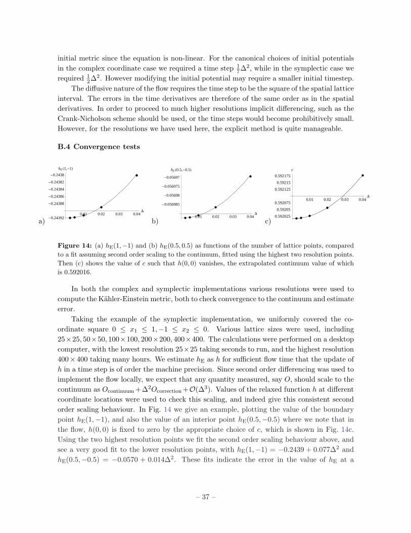
initial metric since the equation is non-linear. For the canonical choices of initial potentialsin the complex coordinate case we required a time step 1
7∆2, while in the symplectic case werequired 1
2∆2. However modifying the initial potential may require a smaller initial timestep.The diffusive nature of the flow requires the time step to be the square of the spatial lattice
interval. The errors in the time derivatives are therefore of the same order as in the spatialderivatives. In order to proceed to much higher resolutions implicit differencing, such as theCrank-Nicholson scheme should be used, or the time steps would become prohibitively small.However, for the resolutions we have used here, the explicit method is quite manageable.
B.4 Convergence tests
a)0.01 0.02 0.03 0.04
D
-0.24392
-0.24388
-0.24386
-0.24384
-0.24382
-0.2438
hE H1,-1L
b)0.01 0.02 0.03 0.04
D
-0.056985
-0.05698
-0.056975
-0.05697
hE H0.5,-0.5L
c)
0.01 0.02 0.03 0.04D
0.592025
0.59205
0.592075
0.592125
0.59215
0.592175
c
Figure 14: (a) hE(1,−1) and (b) hE(0.5, 0.5) as functions of the number of lattice points, comparedto a fit assuming second order scaling to the continuum, fitted using the highest two resolution points.Then (c) shows the value of c such that h(0, 0) vanishes, the extrapolated continuum value of whichis 0.592016.
In both the complex and symplectic implementations various resolutions were used tocompute the Kahler-Einstein metric, both to check convergence to the continuum and estimateerror.
Taking the example of the symplectic implementation, we uniformly covered the co-ordinate square 0 ≤ x1 ≤ 1,−1 ≤ x2 ≤ 0. Various lattice sizes were used, including25×25, 50×50, 100×100, 200×200, 400×400. The calculations were performed on a desktopcomputer, with the lowest resolution 25×25 taking seconds to run, and the highest resolution400× 400 taking many hours. We estimate hE as h for sufficient flow time that the update ofh in a time step is of order the machine precision. Since second order differencing was used toimplement the flow locally, we expect that any quantity measured, say O, should scale to thecontinuum as Ocontinuum +∆2Ocorrection +O(∆3). Values of the relaxed function h at differentcoordinate locations were used to check this scaling, and indeed give this consistent secondorder scaling behaviour. In Fig. 14 we give an example, plotting the value of the boundarypoint hE(1,−1), and also the value of an interior point hE(0.5,−0.5) where we note that inthe flow, h(0, 0) is fixed to zero by the appropriate choice of c, which is shown in Fig. 14c.Using the two highest resolution points we fit the second order scaling behaviour above, andsee a very good fit to the lower resolution points, with hE(1,−1) = −0.2439 + 0.077∆2 andhE(0.5,−0.5) = −0.0570 + 0.014∆2. These fits indicate the error in the value of hE at a
– 37 –

point is about 10−6 for the highest resolution 400 × 400 grid calculated in the symplecticimplementation.
0.005 0.01 0.015 0.02 0.025 0.03D
0.2960250.29605
0.296075
0.2961250.29615
0.296175
fH1,1L
Figure 15: A plot of the value of the Kahler potential at the center of the hexagon as a function of∆. The four data points correspond to our 40×40, 80×80, 160×160, and 250×250 grids. The linearfit was made with the two data points with smallest ∆, giving 0.296008 + 0.1898∆2
Likewise in the complex coordinate implementation, various resolutions were computed,up to 250 × 250. The value of the potential at the center of the hexagon, (ξ = 1, η = 1) isplotted in Fig. 15 and we see that the convergence to the continuum value is quadratic in ∆,again consistent with the second order spatial finite differencing. This and other such testssuggest our best 250× 250 grid in the complex case is accurate to about a part in 105.
Note that in both the symplectic and com-
0.01 0.02 0.03 0.04D
-6.334
-6.332
-6.328
-6.326
-6.324
-6.322
-6.32
Λ
Figure 16: The eigenvalue as a function ofnumber of lattice points for the lowest non-constant eigenfunction which transforms triv-ially under the hexagon and U(1)×U(1) sym-metry. Again we see good agreement with asecond order scaling fit function.
plex coordinates, the value of 2f+c at the centerof the hexagon was found to be 0.592016.
The diffusion flow used to study the eigen-functions of the scalar Laplacian was also differ-enced to second order accuracy. The flow wassimulated using the same explicit method, withtime step 1
2∆2, and for the same resolutions asabove. Using the lowest non-constant eigenfunc-tion which transforms trivially under the actionof the U(1)2 and D6 isometries, we plot in Fig. 16the eigenvalue extracted for different resolutions,using the same initial data for the diffusion, andagain fitting second order scaling to the two high-est resolutions. We see consistent second orderscaling behaviour.
– 38 –

C. D6-invariant polynomials
In this section, we describe the set of polynomials
P =∑n,m
bn,mxn1x
m2 (C.1)
invariant under the dihedral group acting on the hexagon.Our dihedral group is generated by two elements R1 and R2 (see (3.50)). If we take a
linear combination of the xi, v · x, then Ri(v · x) = v · Ri · x = (Rtiv) · x, i.e the Ri act on v
by their transpose.Now, R2 has eigenvalues eπi/3 and e−πi/3. A convenient basis of eigenvectors is
v1 = (eπi/6, e−πi/6) ,
v2 = (e−πi/6, eπi/6) .
The basis is convenient because a polynomial that is symmetric in a1 ≡ v1 · x and a2 ≡ v2 · xis symmetric in x1 and x2.
Consider the polynomial
P =∑n,m
cn,man1a
m2 . (C.2)
Symmetry under interchange of a1 and a2 requires cn,m = cm,n. Moreover, we have
R2(an1am2 ) = exp
(πi
3(n−m)
)an1a
m2 (C.3)
which implies that n−m ≡ 0 mod 6. We conclude that the most general polynomial invariantunder the group action can be decomposed into a sum of polynomials of the form an1a
m2 +am1 a
n2
where n−m ≡ 0 mod 6.For example, two important invariant polynomials are
a1a2 = x21 + x1x2 + x2
2 ≡ U ,
127
(a31 + a3
2)2 = x2
1x22(x1 + x2)2 ≡ V .
We now argue that any invariant polynomial can be decomposed into sums and productsof U and V . Assume an1a
m2 + am1 a
n2 is left invariant by R2 and assume m is the minimum of
m and n. Then
an1am2 + am1 a
n2 = (a1a2)m(an−m1 + an−m2 ) = Um(an−m1 + an−m2 )
One can prove inductively that an−m1 + an−m2 can be written in terms of U and V whenever(n−m) is a multiple of 6. So U and V generate the polynomials invariant under R1 and R2.
– 39 –

D. Convergence and error estimates of the constrained optimization method
In this appendix we give convergence results for the smooth part of the symplectic potential,h(x1, x2) determined in Section 6. At all points in the hexagon domain the value of h wasobserved to converge quickly with increasing numbers of terms taken in the series expansionat the origin. In Fig. 17 we plot the value of h at 3 points. Note that one of these pointslies on the boundary of the hexagon. All other points checked, both in the hexagon interiorand on the boundary, gave qualitatively similar convergence. In the figure we also comparethe data with the extrapolated continuum results for the Ricci flow given in the previousappendix (suitably adjusting for the different value of c). We see excellent agreement. Wemay also estimate that the eighteenth order results and the estimated infinite order resultdiffer at the 1 part in 106 level.
a) 2 4 6 8 10 12 14 16 18n-0.2962
-0.296
-0.2958
-0.2956
-0.2954
-0.2952
-0.295
-0.2948
h@0,0D
b) 2 4 6 8 10 12 14 16 18n
-0.353
-0.3528
-0.3526
-0.3524
-0.3522
-0.352
[email protected],-0.5D
c) 2 4 6 8 10 12 14 16 18n-0.54
-0.5399
-0.5398
-0.5397
-0.5396
-0.5395h@1,-1D
Figure 17: (a) h(0, 0), (a) h(0.5,−0.5) and (b) h(1,−1) as functions of the number terms in theexpansion. The dashed lines show the extrapolated continuum from the Ricci flow results.
References
[1] S.-T. Yau, “Calabi’s Conjecture and some new results in algebraic geometry,” Proc. Nat. Acad.Sci. 74, 1798 (1977);S.-T. Yau, “On the Ricci curvature of a compact Kahler manifold and the complexMonge-Ampere equations,” Comm. Pure App. Math. 31, 339-411 (1978).
[2] M. Headrick and T. Wiseman, “Numerical Ricci-flat metrics on K3,” Class. Quant. Grav. 22,4931 (2005) [arXiv:hep-th/0506129].
[3] S. Donaldson, “Some numerical results in complex differential geometry,”arXiv:math.DG/0512625.
[4] M. R. Douglas, R. L. Karp, S. Lukic and R. Reinbacher, “Numerical Calabi-Yau metrics,”arXiv:hep-th/0612075.
[5] M. R. Douglas, R. L. Karp, S. Lukic and R. Reinbacher, “Numerical solution to the hermitianYang-Mills equation on the Fermat quintic,” arXiv:hep-th/0606261.
[6] G. Tian, “On Kahler-Einstein metrics on certain Kahler manifolds with c1(M) > 0,” Invent.Math. 89 (1987) 225-246;G. Tian and S. T. Yau, “On Kahler-Einstein metrics on complex surfaces with C1 > 0,”Commun. Math. Phys. 112 (1987) 175-203.
– 40 –
[7] Y.T. Siu, “The existence of Kahler-Einstein metrics on manifolds with positive anticanonicalline bundle and a suitable finite symmetry group” Ann. of Math. (2) 127 (1988), no. 3, 585-627.
[8] B. Feng, A. Hanany and Y. H. He, “Phase structure of D-brane gauge theories and toricduality,” JHEP 0108, 040 (2001) [arXiv:hep-th/0104259].
[9] A. Hanany and A. Iqbal, “Quiver theories from D6-branes via mirror symmetry,” JHEP 0204,009 (2002) [arXiv:hep-th/0108137].
[10] C. E. Beasley and M. R. Plesser, “Toric duality is Seiberg duality,” JHEP 0112, 001 (2001)[arXiv:hep-th/0109053].
[11] I. R. Klebanov and A. A. Tseytlin, “Gravity duals of supersymmetric SU(N) x SU(N+M) gaugetheories,” Nucl. Phys. B 578, 123 (2000) [arXiv:hep-th/0002159].
[12] I. R. Klebanov and M. J. Strassler, “Supergravity and a confining gauge theory: Dualitycascades and chiSB-resolution of naked singularities,” JHEP 0008, 052 (2000)[arXiv:hep-th/0007191].
[13] M. Abreu, “Kahler geometry of toric manifolds in symplectic coordinates,” to appear in ToricVarieties in Algebraic Geometry and Physics V. Batyrev (ed.), AMS, math.DG/0004122
[14] G. Tian and X. Zhu, “Convergence of Kahler-Ricci Flow,” J. Amer. Math. Soc., posted Nov17 2006, S-0894-0347(06)00552-2 (2006)
[15] K. Hori and A. Kapustin, “Duality of the fermionic 2d black hole and N = 2 Liouville theory asJHEP 0108, 045 (2001) [arXiv:hep-th/0104202].
[16] D. Garfinkle and J. Isenberg, “Critical behavior in Ricci flow,” arXiv:math.DG/0306129;D. Garfinkle and J. Isenberg, “Numerical studies of the behavior of Ricci flow,” in Geometricevolution equations, vol. 367 of Contemp. Math., pp. 1-3–114. Amer. Math. Soc., Providence,RI, 2005.
[17] M. Headrick and T. Wiseman, “Ricci flow and black holes,” Class. Quant. Grav. 23, 6683(2006) [arXiv:hep-th/0606086].
[18] M. Headrick and T. Wiseman, to appear
[19] X. Wang and X. Zhu, “Kahler-Ricci solitons on toric manifolds with positive first Chern Class,”Adv. Math. 188 (2004) no. 1, 87-103
[20] V. Baytrev and E. Selivanova, “Einstein-Kahler metrics on symmetric toric Fano manifolds,” J.Reine. Agnew. Math. 512 (1999), 225-236.
[21] www.stanford.edu/˜headrick/dP3/www.phys.washington.edu/˜herzog/dP3/
[22] S. Donaldson and J. Keller, to appear
[23] S. B. Giddings, S. Kachru and J. Polchinski, “Hierarchies from fluxes in stringcompactifications,” Phys. Rev. D 66, 106006 (2002) [arXiv:hep-th/0105097].
[24] S. Kachru, R. Kallosh, A. Linde and S. P. Trivedi, “De Sitter vacua in string theory,” Phys.Rev. D 68, 046005 (2003) [arXiv:hep-th/0301240].
[25] S. Kachru, R. Kallosh, A. Linde, J. M. Maldacena, L. McAllister and S. P. Trivedi, “Towardsinflation in string theory,” JCAP 0310, 013 (2003) [arXiv:hep-th/0308055].
– 41 –

[26] E. J. Copeland, R. C. Myers and J. Polchinski, “Cosmic F- and D-strings,” JHEP 0406, 013(2004) [arXiv:hep-th/0312067].
[27] K. Altmann, “The versal deformation of an isolated toric Gorenstein singularity,”arXiv:alg-geom/9403004.
[28] D. Berenstein, C. P. Herzog, P. Ouyang and S. Pinansky, “Supersymmetry breaking from aCalabi-Yau singularity,” JHEP 0509, 084 (2005) [arXiv:hep-th/0505029].
[29] S. Franco, A. Hanany, F. Saad and A. M. Uranga, “Fractional branes and dynamicalsupersymmetry breaking,” JHEP 0601, 011 (2006) [arXiv:hep-th/0505040].
[30] M. Bertolini, F. Bigazzi and A. L. Cotrone, “Supersymmetry breaking at the end of a cascade ofSeiberg dualities,” Phys. Rev. D 72, 061902 (2005) [arXiv:hep-th/0505055].
[31] M. Grana and J. Polchinski, “Supersymmetric three-form flux perturbations on AdS(5),” Phys.Rev. D 63, 026001 (2001) [arXiv:hep-th/0009211].
[32] Y. Matsushima, “Sur la structure du groupe d’homeomorphismes analytiques d’une certainevariete kaehlerienne,” Nagoya Math. J. 11 (1957), 145-150.
[33] S. Franco, Y. H. He, C. Herzog and J. Walcher, “Chaotic duality in string theory,” Phys. Rev.D 70, 046006 (2004) [arXiv:hep-th/0402120];S. Franco, Y. H. He, C. Herzog and J. Walcher, “Chaotic cascades for D-branes onsingularities,” arXiv:hep-th/0412207.
[34] C. P. Herzog, Q. J. Ejaz and I. R. Klebanov, “Cascading RG flows from new Sasaki-Einsteinmanifolds,” JHEP 0502, 009 (2005) [arXiv:hep-th/0412193].
[35] C. P. Herzog and I. R. Klebanov, “On string tensions in supersymmetric SU(M) gauge theory,”Phys. Lett. B 526, 388 (2002) [arXiv:hep-th/0111078].
[36] V. Guillemin, “Kahler structures on toric varieties,” J. Diff. Geom. 40 (1994) 285-309.
[37] W. Fulton, Introduction to Toric Varieties, Princeton University Press, 1993, p 92.
– 42 –