NORTHEASTERN UNIVERSITY · Northeastern University Boston, Massachusetts September 2000. Abstract Applications, and their associated programming models, have had a profound inﬂuence

NORTHEASTERN UNIVERSITYGraduate School of Engineering

Thesis Title: Microarchitectural and Compile-Time Optimizations for Performance Improvement of Procedu-

ral and Object-Oriented Languages.

Author: John Kalamatianos.

Department: Electrical and Computer Engineering.

Approved for Thesis Requirements of the Doctor of Philosophy Degree:

Thesis Advisor: Professor David R. Kaeli Date

Thesis Committee: Professor Waleed Meleis Date

Thesis Committee: Dr. Joel Emer Date

Thesis Committee: Professor Augustus Uht Date

Chairman of Department: Professor Fabricio Lombardi Date

Graduate School Notified of Acceptance:

Associate Dean of Engineering: Yaman Yener Date

MICROARCHITECTURAL AND COMPILE-TIME OPTIMIZATIONS FOR

PERFORMANCE IMPROVEMENT OF PROCEDURAL AND

OBJECT-ORIENTED LANGUAGES

A Thesis Presented

by

John Kalamatianos

to

The Department of Electrical and Computer Engineering

in partial fulfillment of the requirements

for the degree of

Doctor in Philosophy

in the field of

Electrical Engineering

Northeastern University

Boston, Massachusetts

September 2000

Abstract

Applications, and their associated programming models, have had a profound influence on computer archi-

tecture evolution. Programs developed in procedural languages (e.g., C and fortran) have traditionally served

this role. The popularity of the Object Oriented Programming (OOP) paradigm has been growing rapidly,

especially through the use of languages such as C++ and Java.OOP languages support the concepts of data

encapsulation, polymorphism and inheritance, which promise to increase code reuse and result in more reliable

code. Applications developed in object oriented languagesexhibit different execution behavior compared to

their procedural language counterparts.

We focus our work on two primary differences encountered as we move to applications developed in OO

languages: i) the increased number of procedures and their higher calling frequencies, and ii) the increased use

of indirect branches. Equipped with a set of C and C++ benchmark applications, we propose microarchitectural

mechanisms and compiler optimizations to alleviate performance bottlenecks presented by both programming

models. We perform our evaluation in the context of multiple-issue, dynamically scheduled, microprocessors,

and their associated memory hierarchies.

To improve procedure layout on the memory space, we propose agraph-based model that exploits temporal

procedure interaction at a broader scale than a traditionalCall Graph. The model is used to guide a cache

conscious procedure placement algorithm. We evaluate the effectiveness of this algorithm, when combined

with intraprocedural basic block reordering. Our algorithm is aimed at reducing the number of conflict misses

in a multi-level cache hierarchy.

In the field of indirect branches, we classify the statistical behavior and predictability of indirect branches

based on their source code usage. We describe a hardware-based indirect branch prediction scheme that exploits

both multiple path-length correlation and run-time selection of correlation type. We assess the performance of

our scheme compared to a variety of predictors, and also address the cost-effectiveness of indirect branch

prediction.

Contents

Bibliography iii

1 Introduction 1

1.1 Problem Statement . . . . . . . . . . . . . . . . . . . . . . . . . . . . . . . .. . . . . . . . 2

1.1.1 Characteristics of Object-Oriented languages . . . . .. . . . . . . . . . . . . . . . . 2

1.2 Dealing with Instruction Memory Access . . . . . . . . . . . . . .. . . . . . . . . . . . . . 5

1.3 Dealing with Indirect Branches . . . . . . . . . . . . . . . . . . . . .. . . . . . . . . . . . 6

1.4 Experimental Approach . . . . . . . . . . . . . . . . . . . . . . . . . . . .. . . . . . . . . 7

1.5 Contributions . . . . . . . . . . . . . . . . . . . . . . . . . . . . . . . . . . .. . . . . . . . 9

1.6 Overview . . . . . . . . . . . . . . . . . . . . . . . . . . . . . . . . . . . . . . . .. . . . . 9

2 Code Reordering for Single Level Caches 11

2.1 Related Work . . . . . . . . . . . . . . . . . . . . . . . . . . . . . . . . . . . . .. . . . . . 11

2.2 Capturing Temporal Procedure Interaction . . . . . . . . . . .. . . . . . . . . . . . . . . . 16

2.2.1 Procedure-based Inter-Reference Gap Modeling . . . . .. . . . . . . . . . . . . . . 21

2.3 Pruning Algorithm . . . . . . . . . . . . . . . . . . . . . . . . . . . . . . . .. . . . . . . . 28

2.4 Cache-Sensitive Procedure Reordering Algorithm . . . . .. . . . . . . . . . . . . . . . . . . 30

2.4.1 Complexity Analysis . . . . . . . . . . . . . . . . . . . . . . . . . . . .. . . . . . . 34

2.5 Main Memory-based Procedure Placement Algorithm . . . . .. . . . . . . . . . . . . . . . 36


2.6 Intraprocedural Basic Block Reordering Algorithm . . . .. . . . . . . . . . . . . . . . . . . 40

2.7 Experimental Results . . . . . . . . . . . . . . . . . . . . . . . . . . . . .. . . . . . . . . . 47

2.8 Summary . . . . . . . . . . . . . . . . . . . . . . . . . . . . . . . . . . . . . . . . .. . . . 59

3 Code Reordering for Multiple Level Caches 60

3.1 Related Work . . . . . . . . . . . . . . . . . . . . . . . . . . . . . . . . . . . . .. . . . . . 60

i

3.2 Cache-Sensitive Procedure Reordering Algorithm . . . . .. . . . . . . . . . . . . . . . . . . 61


3.3 Main Memory-based Procedure Placement Algorithm . . . . .. . . . . . . . . . . . . . . . 67



3.5 Summary . . . . . . . . . . . . . . . . . . . . . . . . . . . . . . . . . . . . . . . . .. . . . 80

4 Indirect Branch Classification and Characterization 81

4.1 Related Work . . . . . . . . . . . . . . . . . . . . . . . . . . . . . . . . . . . . .. . . . . . 81

4.2 Opcode and Source Code-based Indirect Branch Classification . . . . . . . . . . . . . . . . . 83

4.2.1 Conventional function calls . . . . . . . . . . . . . . . . . . . . .. . . . . . . . . . 83

4.2.2 Virtual function calls . . . . . . . . . . . . . . . . . . . . . . . . . .. . . . . . . . . 84

4.2.3 Switch statements . . . . . . . . . . . . . . . . . . . . . . . . . . . . . .. . . . . . 94

4.2.4 Target-based compile-time classification . . . . . . . . .. . . . . . . . . . . . . . . . 95

4.3 Profile-based Classification . . . . . . . . . . . . . . . . . . . . . . .. . . . . . . . . . . . 97

4.3.1 Target-based profile-guided classification . . . . . . . .. . . . . . . . . . . . . . . . 98

4.3.2 Correlation-based classification . . . . . . . . . . . . . . . .. . . . . . . . . . . . . 104

4.4 Load-based Characterization . . . . . . . . . . . . . . . . . . . . . .. . . . . . . . . . . . . 112

4.5 Summary . . . . . . . . . . . . . . . . . . . . . . . . . . . . . . . . . . . . . . . . .. . . . 117

5 Indirect Branch Prediction Mechanisms 118

5.1 Related Work . . . . . . . . . . . . . . . . . . . . . . . . . . . . . . . . . . . . .. . . . . . 118

5.2 Data Compression Algorithms and Branch Prediction . . . .. . . . . . . . . . . . . . . . . . 121

5.3 PPM-based Indirect Branch Predictors . . . . . . . . . . . . . . .. . . . . . . . . . . . . . . 125

5.4 Load Latency Tolerance and Indirect Branches . . . . . . . . .. . . . . . . . . . . . . . . . 130

5.5 Temporal Reuse of Indirect Branches . . . . . . . . . . . . . . . . .. . . . . . . . . . . . . 140


5.7 Summary . . . . . . . . . . . . . . . . . . . . . . . . . . . . . . . . . . . . . . . . .. . . . 158

6 Conclusions and Future Work 159

6.1 Contributions . . . . . . . . . . . . . . . . . . . . . . . . . . . . . . . . . . .. . . . . . . . 159

6.2 Future Research on Code Reordering . . . . . . . . . . . . . . . . . .. . . . . . . . . . . . 160

6.3 Future Research on Indirect Branch Prediction . . . . . . . .. . . . . . . . . . . . . . . . . 161

A 164

ii

B 170

C 176

D 180

Bibliography 183

iii

List of Figures

2.1 Call Graph used as an example towards highlighting different types of procedure interaction. . 16

2.2 CMG construction algorithm. . . . . . . . . . . . . . . . . . . . . . . .. . . . . . . . . . . . 19

2.3 LRU stack of size 4 and procedure list content snapshots for the profile information shown at

the left column. . . . . . . . . . . . . . . . . . . . . . . . . . . . . . . . . . . . . .. . . . . 20

2.4 Edge ordering comparison between the TRG and CMG (upper left corner plot), the CG and

the TRG (upper right corner plot) and the CG with the CMG (centered plot). All graphs are

generated with profile information extracted from the ixx benchmark. . . . . . . . . . . . . . 25

2.5 Edge ordering comparison between the TRG and CMG (upper left corner plot), the CG and

the TRG (upper right corner plot) and the CG with the CMG (centered plot). All graphs are

generated with profile information extracted from the eqn benchmark. . . . . . . . . . . . . . 26

2.6 Computing the degree of overlap between procedures in the cache address space. . . . . . . . 31

2.7 Single-level cache line coloring algorithm. . . . . . . . . .. . . . . . . . . . . . . . . . . . . 33

2.8 Popular procedure memory placement algorithm after performing single-level cache coloring. 37

2.9 Scenarios where code size can increase in the presence/absence of basic block reordering. . . . 39

2.10 Basic block placement decisions during intraprocedural basic block reordering. . . . . . . . . 42

2.11 Algorithm that virtually partitions a procedure into ahot and a cold region after applying in-

traprocedural basic block reordering. . . . . . . . . . . . . . . . . .. . . . . . . . . . . . . . 44

2.12 Code fix-up steps after applying intraprocedural basicblock reordering. . . . . . . . . . . . . 45

2.13 Cycle count reduction/increase after applying singlecache level code reordering to the default

code layout. All results are generated via execution-driven simulation. . . . . . . . . . . . . . 52

2.14 Memory cycle count reduction/increase after applyingsingle cache level code reordering to the

default code layout. All results are generated via trace-driven simulation. . . . . . . . . . . . . 53

2.15 L1/L2 cache miss ratios of both the optimized and the unoptimized executables. The number

of references to L1/L2 is appended on top of every bar. All results are generated via execution-

driven simulation. . . . . . . . . . . . . . . . . . . . . . . . . . . . . . . . . . .. . . . . . . 54

iv

2.16 L1/L2 cache miss ratios of both the optimized and the unoptimized executables. The number of

references to L2 is also appended on top of every bar. All results are generated via trace-driven

simulation. . . . . . . . . . . . . . . . . . . . . . . . . . . . . . . . . . . . . . . . .. . . . 55

3.1 Different coloring scenarios considering two cache levels wherek =j log2(L2ls)�log2(L1ls) jandl =j (log2(SL2) + log2(L2ls))� (log2(SL1) + log2(L1ls)) j. . . . . . . . . . . . . . . . 63

3.2 Multiple-level cache line coloring algorithm. . . . . . . .. . . . . . . . . . . . . . . . . . . . 65

3.3 Multiple-level cache line coloring algorithm (continued). . . . . . . . . . . . . . . . . . . . . 66

3.4 Popular procedure memory placement algorithm after performing two-level cache coloring

(continued). . . . . . . . . . . . . . . . . . . . . . . . . . . . . . . . . . . . . . . .. . . . . 68

3.5 Popular procedure memory placement algorithm after performing two-level cache coloring. . . 69

3.6 Cycle count reduction/increase after applying two-level cache code reordering to the default

code layout. All results are generated via execution-driven simulation. . . . . . . . . . . . . . 73

3.7 Memory cycle count reduction/increase after applying two-level cache code reordering to the

default code layout. All results are generated via trace-driven simulation. . . . . . . . . . . . . 74

3.8 Comparison of the cycle count reduction after applying single and two-level cache code re-

ordering to the default code layout. The set of results shownon the left (right) is generated via

execution-driven (trace-driven) simulation. . . . . . . . . . .. . . . . . . . . . . . . . . . . . 75

3.9 L1/L2 cache miss ratios of both the optimized and the unoptimized executables. The number

of references to L1/L2 is appended on top of every bar. All results are generated via execution-

driven simulation. . . . . . . . . . . . . . . . . . . . . . . . . . . . . . . . . . .. . . . . . . 77

3.10 L1/L2 cache miss ratios of both the optimized and the unoptimized executables. The number of

references to L2 is also appended on top of every bar. All results are generated via trace-driven

simulation. . . . . . . . . . . . . . . . . . . . . . . . . . . . . . . . . . . . . . . . .. . . . 78

4.1 Object layout for class hierarchies with single, multiple and virtual inheritance. . . . . . . . . 85

4.2 Visibility rules for C++ virtual function call resolution. . . . . . . . . . . . . . . . . . . . . . 87

4.3 Object layout in the presence of virtual functions, inside a class hierarchy with single, multiple

and virtual inheritance. . . . . . . . . . . . . . . . . . . . . . . . . . . . . .. . . . . . . . . 88

4.4 Memory layout of the four VFT configurations for an objectof a class that exercises both

multiple and virtual inheritance. . . . . . . . . . . . . . . . . . . . . .. . . . . . . . . . . . 91

4.5 Range of classes associated with a virtual function call: I is the introducing class forfoo, Eis the class that definesfoo, S;D are the classes that the pointer callingfoo points at compile

and run-time respectively. . . . . . . . . . . . . . . . . . . . . . . . . . . .. . . . . . . . . . 92

v

4.6 Example illustrating how the virtual function call mechanism invokes two different implemen-

tations of a function. . . . . . . . . . . . . . . . . . . . . . . . . . . . . . . . .. . . . . . . 93

4.7 Dynamic counts of Monomorphic, Polymorphic and Megamorphic MT jmp, VF jsr and FP jsr

branches. . . . . . . . . . . . . . . . . . . . . . . . . . . . . . . . . . . . . . . . . . .. . . 99

4.8 Prediction ratio of MT jmp, VF jsr and FP jsr branches using a predictor where every per-branch

entry consists of a 4-wide LRU buffer storing past targets for that branch. . . . . . . . . . . . 100

4.9 Dynamic counts of LEB, MEB and HEB MT jmp, VF jsr and FP jsr branches. . . . . . . . . . 102

4.10 Misprediction ratios of MT indirect branch classes with path correlation lengths of 0, 4, 8 and 12.108

4.11 Cold-start misprediction ratios of MT indirect branches with path correlation lengths of 0, 4, 8

and 12. . . . . . . . . . . . . . . . . . . . . . . . . . . . . . . . . . . . . . . . . . . . . .. . 113

4.12 Dynamic counts of Monomorphic, Polymorphic and Megamorphic ib-loads associated with VF

jsr, FP jsr and MT jmp branches. . . . . . . . . . . . . . . . . . . . . . . . . .. . . . . . . . 115

4.13 L1 D-cache misses due to ib-loads associated with VF jsr, FP jsr and MT jmp branches. . . . . 116

5.1 Prediction algorithm for a 4th order PPM predictor as it applies to conditional branch prediction. 124

5.2 Select-Fold-Shift-XOR-Select (SFSXS) indexing function as it applies to the contents of a PHR. 126

5.3 Single-level access implementation of a 4th order PPM predictor. It uses a set of BTBs to

implement the Markov components. Each component is indexedwith a variable number of

targets, extracted from a single PHR. . . . . . . . . . . . . . . . . . . .. . . . . . . . . . . . 127

5.4 PPM predictor with run-time selection of correlation type. Two PHRs are used to record path

history of PIB and PB type. Two-bit counters, kept on an indirect branch basis, select the PHR

at run-time. . . . . . . . . . . . . . . . . . . . . . . . . . . . . . . . . . . . . . . . .. . . . 129

5.5 State machine of a 2-bit up/down saturating counter. Thecounter is used to select one of the

two available PHRs in a scheme that combines PPM prediction with run-time selection of path

history type. . . . . . . . . . . . . . . . . . . . . . . . . . . . . . . . . . . . . . . .. . . . . 130

5.6 Indirect branch format in the Alpha ISA. . . . . . . . . . . . . . .. . . . . . . . . . . . . . . 132

5.7 Ibload encoding scheme for the indirect branch instruction of the Alpha ISA. The example

shows the encoding of two ibloads using the displacement field of the indirect branch. . . . . . 133

5.8 Update protocol of the load tolerance counter. Solid lines model transitions triggered by a cache

miss while dotted lines model transitions triggered by a cache hit. . . . . . . . . . . . . . . . 135

5.9 Phase 1: when an ibload is executed the dependence between the ibload and the indirect branch

is recorded in the DTBL. . . . . . . . . . . . . . . . . . . . . . . . . . . . . . . .. . . . . . 136

vi

5.10 Phase 2: when an ibload is executed we update the DTBL in case its dependence has not already

been recorded. The LMT is updated independently of the DTBL.. . . . . . . . . . . . . . . . 137

5.11 Phase 2: On a D-cache transaction we update the LMT. The DTBL is accessed with the address

being replaced from the D-cache. All branches found in the DTBL set may update the LMT. . 138

5.12 Updating the TLR counters using both the newly arrived target and the target being displaced

from the TLR. . . . . . . . . . . . . . . . . . . . . . . . . . . . . . . . . . . . . . . . .. . . 141

5.13 Cycle count reduction/increase when explicitly usingIB predictors for predicting indirect branches

other than returns. All results are generated with execution-driven simulation and include spec-

ulative traffic. . . . . . . . . . . . . . . . . . . . . . . . . . . . . . . . . . . . . .. . . . . . 145

5.14 Conditional and Indirect branch misprediction ratio over time for the edg benchmark. The ratios

are for the base machine (left side) and a machine using a PPM predictor (right side). . . . . . 146

5.15 Conditional and Indirect branch misprediction ratio over time for the perl benchmark. The

ratios are for the base machine (left side) and a machine using a PPM predictor (right side). . . 148

5.16 Conditional and indirect branch dynamic counts over time for perl (left side) and edg (right

side). All results are generated on a base machine (no IB predictor). . . . . . . . . . . . . . . 148

5.17 Misprediction ratios of various IB predictors. All results are generated with execution-driven

simulation. All predictors are updated speculatively. . . .. . . . . . . . . . . . . . . . . . . . 150

5.18 Average I-fetch queue and instruction window occupancy in the presence of IB prediction.

Results are presented for a machine with either a conservative (lower 7 rows) or an aggressive

fetch unit (upper 7 rows). . . . . . . . . . . . . . . . . . . . . . . . . . . . . .. . . . . . . . 153

vii

List of Tables

1.1 C and C++ benchmark suite description. . . . . . . . . . . . . . . .. . . . . . . . . . . . . . 8

2.1 Edge-related statistics: number of edges for CG, TRG andCMG (columns 2-4) and number of

popular edges for CG, TRG and CMG (columns 5-7). . . . . . . . . . . .. . . . . . . . . . . 29

2.2 Procedure-related statistics: static procedure count(column 2), number of activated procedures

(column 2 in parenthesis), average static popular procedure size in Kb for CG, TRG and CMG

(columns 3-5) and number of popular procedures for CG, TRG and CMG (columns 6-8). . . . 30

2.3 Visiting frequency of each case in the single-level cache line coloring algorithm (columns 2-5).

The number in parentheses in column 5 represents the number of times two procedures of the

same compound node need to be recolored because of conflicts.. . . . . . . . . . . . . . . . 35

2.4 Size of memory gaps after single-level cache coloring and memory placement using the CG,

TRG or the CMG. The total gap size is shown before (columns 2-5) and after (columns 6-8)

mapping unactivated and unpopular procedures. Each columndisplays the gap size when basic

block reordering does not apply and when it precedes cache coloring. . . . . . . . . . . . . . 38

2.5 Statistics associated with basic block repositioning:number of introduced unconditional branches

(column 2) and subset of those which form a basic block (column 2, in parentheses), number

of deleted unconditional branches (column 3), number of conditional branches whose opcode

has been switched (column 4), average DCFG size in basic blocks (column 5), average DCFG

size in Kbytes (column 6), total HR size in Kbytes (column 7) and average HR size in bytes

(column 8). . . . . . . . . . . . . . . . . . . . . . . . . . . . . . . . . . . . . . . . . .. . . 46

2.6 Dynamically scheduled, Out-Of-Order, multiple issue machine description. . . . . . . . . . . 48

2.7 Total number of executed instructions (column 2). Instructions per Cycle (IPC) for single cache

level coloring code reordering configurations (columns 3-9, rows 1-5). Memory Cycles per

Instruction (MCPI) for single cache level coloring code reordering configurations (columns

3-9, rows 6-11). . . . . . . . . . . . . . . . . . . . . . . . . . . . . . . . . . . . . .. . . . . 49

viii

2.8 I-TLB misses and number of allocated pages for both the unoptimized case and the executables

optimized with different configurations of single level cache code reordering. . . . . . . . . . 56

2.9 Number of committed/executed instructions for both theunoptimized case and the executables

optimized with different configurations of single level cache code reordering. . . . . . . . . . 57

2.10 Average Instruction window and Instruction fetch queue size for both the unoptimized case and

the executables optimized with different configurations ofsingle level cache code reordering. . 58

2.11 Number of conditional branches that were committed andfound to be taken for both the unop-

timized case and the executables optimized with different configurations of single level cache

code reordering. . . . . . . . . . . . . . . . . . . . . . . . . . . . . . . . . . . . .. . . . . . 59

3.1 Size of memory gaps after two-level cache coloring and memory placement using the CG, TRG

or the CMG. The total gap size is shown before (columns 2-5) and after (columns 6-8) mapping

unactivated and unpopular procedures. Each column displays the gap size when basic block

reordering does not apply and when it precedes cache coloring. . . . . . . . . . . . . . . . . . 70

3.2 Total number of executed instructions (column 2). Instructions per Cycle (IPC) for two-level

cache coloring code reordering configurations (columns 3-9, rows 1-5). Memory Cycles per

Instruction (MCPI) for two-level cache coloring code reordering configurations (columns 3-9,

rows 6-11). . . . . . . . . . . . . . . . . . . . . . . . . . . . . . . . . . . . . . . . . .. . . 72

3.3 Revealing the amount of L2 color reevaluation: total number of popular procedures for CG,

TRG and CMG (columns 2-4), number of popular procedures subject to L2 color reevaluation

for CG, TRG and CMG, when no bb-reordering has been performed(columns 5-7) and when

bb-reordering precedes two-level cache coloring (columns8-10). . . . . . . . . . . . . . . . . 76

3.4 I-TLB misses and number of allocated pages for both the unoptimized case and the executables

optimized with different configurations of two-level cachecode reordering. . . . . . . . . . . 79

4.1 Run-time statistics for indirect branches: number of instructions (column 2), average number

of instructions per indirect branch (column 3), average number of conditional branches per

indirect branch (column 4), number of static active VF jsr, FP jsr and MT jmp (columns 5, 7,

9), percentage of indirect branches that belong to the VF jsr, FP jsr, MT jmp class (columns 5,

7, 9, in parentheses), average number of targets per indirect branch class (columns 6, 8, 10),

number of static indirect branches whose total dynamic count is 90% and 95% over all indirect

branches (columns 11, 12). . . . . . . . . . . . . . . . . . . . . . . . . . . . .. . . . . . . . 97

4.2 Profile-guided indirect branch classes based on the number of visited targets. . . . . . . . . . 98

4.3 Number of unique Self, PB, PIB and PCB path histories for VF jsr, FP jsr and MT jmp branches.106

ix

4.4 Statistics of ib-load instructions: number of executedloads (column 2), percentage of dynamic

ib-loads over all dynamic loads (column 3), percentage of ib-loads due to VF jsr, FP jsr and

MT jmp over all dynamic loads (columns 4, 6 and 8) and average number of targets per ib-load

accompanying a VF jsr, FP jsr or MT jmp (columns 5, 7 and 9). . . .. . . . . . . . . . . . . 114

5.1 Breakdown of predictions for a Cascaded predictor. The classification includes the total number

of lookups (column 2), the number of lookups made the long path (column 3) and the short

path component (column 4), the number of filter lookups (column 5) and the number of filter

mispredictions (column 6). . . . . . . . . . . . . . . . . . . . . . . . . . . .. . . . . . . . . 151

5.2 Number of mispredictions for a PPM predictor. Column 2 lists the number of tag mismatches

and column 3 includes the number of target mispredictions. .. . . . . . . . . . . . . . . . . . 152

5.3 Number of committed/executed instructions for machines employing IB prediction. The num-

ber of committed instructions is presented in column 2 whilethe number of executed instruc-

tions follows in columns 3-9. . . . . . . . . . . . . . . . . . . . . . . . . . .. . . . . . . . . 154

5.4 L1 I-cache number of accesses and misses for a base machine (column 2) and machines em-

ploying IB prediction (columns 3-8). . . . . . . . . . . . . . . . . . . .. . . . . . . . . . . . 155

5.5 Misprediction ratios for IB predictors with LRU (columns 2-4) and TLR/LMT replacement

policies (columns 5-7). All results are generated using execution-driven simulation. . . . . . . 156

5.6 Breakdown of replacement decisions for IB predictors using the TLR/LMT replacement policy.

Columns 2, 5 and 8 list the total number of replacement decisions. Columns 3, 6 and 9 present

the number of times the TLR/LMT policy deviates from LRU and replaces a branch using the

LMT counters. Columns 4, 7 and 10 present the number of times the TLR/LMT policy deviates

from LRU and replaces a branch using the TLR counters. . . . . . .. . . . . . . . . . . . . . 157

x

Chapter 1

Introduction

Benchmark applications, and their associated programmingmodels, have had a profound influence on computer

architecture and compiler design. Architectural support in the form of microarchitectural mechanisms and

instruction set architecture (ISA) extensions, as well as many compiler optimizations, have been motivated

by studies performed on programs written in procedural languages such as C and/or Fortran [1, 2]. Program

behavior [3, 4] has played and continues to play an importantrole in the evolution of modern architectures [5, 6].

Design decisions in several machines such as the IBM 801, Stanford MIPS and Berkeley RISC projects were

guided by trends found in a set of C, Pascal and FORTRAN programs [2, 7]. The IBM System/360 ISA has been

influenced by frequently used operations in COBOL and FORTRAN applications, such as string manipulation

and floating-point operations [8]. Most recently, microprocessor performance has been evaluated based on the

SPEC92 and SPEC95 benchmarks, a mixture of C and FORTRAN programs [9]. Over the years architectural

trends tailored system design in order to support or directly execute certain programming languages or models

[6, 10, 11]. Most current workload-driven design has focused on improving the performance of FORTRAN and

C programs.

More recently, the Object Oriented Programming paradigm (OOP) has steadily grown in popularity, es-

pecially through the use of languages such as C++ and Java. Concepts such as information hiding, message

passing, polymorphism, inheritance, data abstraction anddata encapsulation promise to revolutionize the way

software will be developed. The software community views OOP as the major vehicle to reduce software

complexity, increase code reuse, reduce maintenance costsand improve the reliability of the delivered binaries

[12]. However, applications developed with the OOP have been found to exhibit different execution behavior

compared to their procedural counterparts, generating additional overhead.

In this work we attempt to investigate the instruction stream behavior of both procedural and object-oriented

programs. We do this in the context of superscalar microprocessors and their associated memory hierarchies. In

1

the software domain, we propose profile-guided code reordering algorithms to reduce the cost associated with

accessing instructions from a modern memory hierarchy consisting of multiple cache levels. Our motivation

stems from the higher static and dynamic procedure count detected in object-oriented applications. In the

hardware domain, we study mechanisms to reduce the penalty incurred by indirect branches, which, among

their other uses, support polymorphic calls in object-oriented applications.

1.1 Problem Statement

The goal of our work is twofold: reduce the cost due to cache conflicts when fetching instructions from the

memory hierarchy and reduce the effects induced by indirectbranches in the presence of control speculation.

Optimizing the overhead of cache conflicts is achieved by statically reorganizing the executable using profile

data. The impact of indirect branches on the sequentiality of control flow is confronted with hardware-based

prediction schemes. These two techniques are evaluated using benchmarks from both the OO and procedural

language domain and experimental results are presented to verify their effectiveness on both types of applica-

tions.

1.1.1 Characteristics of Object-Oriented languages

Given the growing popularity of OOP, it is not surprising that many studies have focused on the behavior of

programs written with object-oriented languages [13, 14, 15, 16, 17]. A significant amount of research has

also dealt with compiler optimizations and architectural support to improve the performance of object-oriented

software [18, 19, 20, 21, 22, 23, 24, 25, 26].

OOP is fundamentally built around the concept of an object and its underlying model. An object is fully

described with its state and the necessary behavior to manipulate that state. Data encapsulation is the property

of combining state and behavior together to represent an object. Objects sharing state and behavior are grouped

into classes1. The behavior of an object is implemented with a set of procedures, while its state is modeled

with a set of variables/data structures. Data encapsulation, enhanced with information hiding and data ab-

straction, promotes the separation between behavior implementation and use. This separation, supported by an

Application Programming Interface (API), is used towards improving software maintainability and reliability

[12, 27].

Inheritance allows different classes to share behavior andstate, thus improving code sharing, reusability,

consistency of interface and rapid software component prototyping. A class inheriting behavior and/or state is

called asubclasswhile the class providing behavior and/or state is called asuperclass. Polymorphism is the1We will use C++ terms throughout this thesis to maintain consistency

2

property of permitting an entity to hold values of differenttypes during the course of execution. Polymorphism

can be expressed either statically or dynamically. An object, a variable or a function can become a polymorphic

entity [12, 28].

In OOP, data structures are typically encapsulated in objects while object behavior and communication

implement functionality. Given the same programming task,(i.e., its algorithms and corresponding data struc-

tures), studies have shown that both the static and dynamic procedure count required to solve the problem tends

to be larger in OOP, as compared to procedural programming. In [13], a detailed comparison between C and

C++ applications was presented. The C++ applications were found to have 3 times as many static procedures

and execute almost 90% more calls than C programs. Objects inOOP are often designed to be generic, allow

code reuse and modularity, and promote information hiding and data abstraction. Each procedure implements

a relatively small and specific part of the behavior for the objects of a class. Consequently, more procedures

are necessary to implement a given task. In addition, programmers tend to fully define behavior in every class,

leading to a larger static count of procedures (methods in C++ parlance). This same property can cause some

procedures or data members to be unreachable or infrequently accessed in a given application [29, 30]. For ex-

ample, in [29], up to 26% of procedures were found to be statically unreachable in C++ applications compared

to only 6% for C applications.

Due to the larger static procedure count, procedures tend topossess a smaller average static size (78 in-

structions for C++ compared to 94 for C, [13]) and a smaller average dynamic size (48 instructions for C++

compared to 153 for C, [13])2. In addition, C++ applications have a slightly smaller average basic block size

(5.4 instructions for C++ and 5.9 for C, [13]). Distributingcontrol flow of an algorithm across a larger number

of procedures is a possible reason behind the smaller basic block size, since loops and if-then-else statements

are frequently partitioned across procedure boundaries. Polymorphism is one feature that tends to substitute

if-then-else constructs with a procedure call [31]. A direct consequence of this is the lower static and dynamic

frequency of conditional branches in OOP [12] (the dynamic frequency of conditional branches was 61% for

C++ and 80% for C in [13]).

Designing object-oriented software, with code reuse and modularity in mind, generated a smaller average

size (3205 bytes for C programs and 171 bytes for C++ [13]) anda larger average count (85% more regions

are allocated in C++ [13]) for dynamically allocated entities. Possible explanations for this phenomenon can

be the heavier use of reusable components which return heap-allocated entities, the tendency of C programs to

use the stack, and the syntactic and semantic conveniences provided by object-oriented languages for dynamic

memory allocation (such as thenewanddeleteoperators and the constructor and destructor methods in C++)

[13]. The larger dynamic procedure count also implies an increased call stack depth (9.9 is the median call2Dynamic procedure size is defined to be the average number of instructions executed, every time a procedure is called.

3

stack depth for C and 12.1 for C++ [13]). Moreover, the C++ programs examined in [13] were typically twice

the size of C programs. Given that the comparison involved application with similar functionality the larger

static code size may be due to the greater fixed calling overhead (percentage of load/stores for restoring/saving

variables and call/return instructions with respect to total number of instructions) and the tendency to provide

more behavior per object than what is actually needed in the application.

A large number of small procedures can have a serious impact on instruction cache performance since

spatial locality tends to drop. Techniques such as code reordering and/or intelligent cache management are

good candidates for improving performance. Dead code and data detection and elimination can help reduce

the code size [29, 30]. Reducing procedure size is importantbecause small procedures can benefit more from

inlining [32] and cloning [33]. Notice, however, that the increased use of indirect branches (which will be

explained below) makes call graph construction and inlining decisions more difficult [34]. The lower static

count of conditional branches, along with the increased frequency of indirect branches, suggest that emphasis

should be placed on indirect branch target prediction.

Furthermore, the data cache traffic and miss ratio is subjectto increases due to the larger number of

load/stores required for saving/restoring variables, polymorphic calls, data member accesses, etc. The larger

number of return instructions and the growing call stack depth is also expected to increase the demand for

hardware predictors such as a Return Address Stack [35]. Thechanges in size and creation rate of dynami-

cally allocated objects may have a negative impact on data caches due to the expected decrease in temporal

(i.e., shorter object lifetime) and spatial (i.e., smallerobject size) locality of data references [36, 37]. Memory

allocators for OOP may need to be redesigned in order to reduce the negative impacts of this trend [38]. A

smaller procedure size indicates a greater need for exploiting inter-procedural ILP by instruction schedulers. In

addition, the use of pointers for accessing object behaviorand state makes aliasing and type analysis even more

critical [22, 39].

Inheritance’s major side effect is that inherited behaviormust be prepared to deal with arbitrary subclasses

and therefore inherited methods are often slower than specialized code [12]. Inherited behavior may increase the

object size by inserting pointers to permit access to inherited methods, by incorporating inherited data members

into a child class object (which may introduce overhead as inthe case of pure abstract base classes) and by

activating padding to allow for aligned accesses to inherited state [40, 28]. Depending on the object layout

construction rules, certain types of inheritance may require additional code overhead when activating behavior

or accessing state [28, 40, 41]. Clearly, all of the above canhave a negative impact on overall performance as

they tend to stress instruction and data caches.

Polymorphism generates run-time overhead by utilizing specialized code sequences to activate behavior

(accessing a data member of an object or calling a polymorphic function). The code sequence, often called

4

dispatch code, varies from language to language. In dynamically typed languages, such as Self, Cecil and

Smalltalk, the overhead is larger than that found in statically typed languages such as C++ and Java. In both

domains, however, polymorphic calls support the generation of high-level reusable software components that

fit different applications, and are therefore frequently encountered.

Dispatch code overhead depends on the underlying run-time mechanisms supporting polymorphic calls

[31]. For C++ (which favors the Virtual Function Table (VFT)as a supporting run-time mechanism for poly-

morphic calls) the dispatch code sequence consists of a few non-branch instructions and an indirect branch

[42]. The non-branch instructions are usually loads, though add operations may also be used, depending on the

ISA [42, 43]. A significant amount of pressure can be applied on the instruction cache and instruction fetch

unit if the dynamic frequency of those polymorphic calls is high [43, 44]. The data cache performance may

also be affected due to the extra memory references. In applications written with dynamically typed languages,

the overhead is even higher, since all operations in a program are implemented as polymorphic calls [45].

Indirect branches are also used to implement dynamically linked library calls (DLL calls), multi-way state-

ments (such as switch statements in C/C++), function pointer-based calls, and calls resulting when the displace-

ment field of conditional branches for a specific ISA can not hold the offset.

1.2 Dealing with Instruction Memory Access

Microprocessor performance continues to grow in part due todynamically scheduling and out-of-order exe-

cution coupled with aggressive forms of control speculation 3. Currently, memory systems have been unable

to keep up with processor request rates. Technology constraints have led to a growing gap between CPU and

DRAM speeds [46]. Given current technology trends, it is likely that future processors will spend a greater

percentage of their time stalled, waiting for data from memory. While latency of data requests can be partially

masked with a plethora of techniques such as prefetching, non-blocking caches, etc., uninterrupted instruction

supply remains a challenge. As processors employ more aggressive forms of control speculation to reveal and

exploit higher degrees of ILP, the number of instructions that need to be supplied from memory in a single clock

cycle will grow. This increased demand can be met by higher instruction cache bandwidth and lower average

response time.

In a hierarchical memory system consisting of multiple cache levels, high-speed first level instruction caches

have typically small degrees of associativity but suffer from a large number of conflicts. Cache misses can occur

because of first-time references (cold-start misses), finite cache capacity (capacity misses) and memory address

conflicts (conflict misses) [47]. Some of the methods that have been proposed for avoiding conflict misses3Our discussion refers to dynamically scheduled, out-of-order machines with no support for multi-threading, data speculation orpredication.

5

are: (i) preventing one code segment from being stored in thecache (cache bypassing [48]), (ii) finding an

alternative place to store the conflicting code module in thecache [49], (iii) implement a mapping function in

hardware so that fewer code modules map to the same cache location [50, 51] and (iv) reorder the code modules

in the main memory address space at compile time so that fewerconflicts may occur at run-time [52, 53, 54].

We pursue the last method.

We first study the temporal interaction among procedures since accurate temporal information has not been

used in the context of code reordering until recently [55]. We then attempt to improve code spatial locality

and instruction fetch efficiency with intraprocedural basic block reordering. A procedure graph, weighted with

temporal information, is subsequently employed to guide a procedure placement algorithm. The algorithm tries

to provide a conflict-free mapping for a predetermined set ofprocedures in the target multi-level cache hierarchy

of the system under investigation. It uses graph coloring toachieve cache-conscious procedure placement.

Laying out code in the main memory address space is the final step. Special care is taken in order to keep the

number of required pages minimal.

1.3 Dealing with Indirect Branches

Microprocessor microarchitecture has seen a long series ofinnovations aimed at producing ever-faster CPUs.

Superscalar processing is just one of these mechanisms. Superscalar processors exploitInstruction Level Par-

allelism (ILP) in the form of issuing multiple instructions per clockcycle [56, 57]. Typically, the instruction

fetch and decode unit constructs a window of instructions that are available for execution. Dedicated hardware

checks for data dependencies between these instructions. The instructions that can be executed simultaneously

are then issued to multiple functional units based on the availability of their operands (data-flow model of ex-

ecution) rather than their original program order. This feature, found in most modern superscalar machines, is

referred to asdynamic scheduling. Completed instructions may retire (update the machine state) based on the

original program order. One of the factors affecting the amount of exploited ILP is the number of instructions

fetched from memory in a single cycle [56]. A steady rate of instruction flow is critical for filling the instruction

window of the processor. Sequential flow is ideal in sustaining a high rate but branches redirect the control flow

breaking the sequentiality. A large number of cycles may then be wasted since the pipeline can not be fed with

instructions until the branch is resolved. An indirect branch is a type of unconditional branch which always

disrupts the sequentiality of the instruction stream.

Speculative executionis an important technique that has been used to overcome the problem of branch

execution redirection. The basic idea is to fetch and execute (but not commit) operations earlier than their

original program order dictates. The benefit may be expressed in the form of a better dynamic schedule or

6

greater tolerance for cache misses, long latency operations or branch redirections. Hardware and software

speculation has been applied in many forms. One widespread form of hardware speculation is predicting the

outcome and target of conditional branches [58]. In our workwe describe a similar form of hardware control

speculation, tailored for indirect branches. In particular, we propose an indirect branch predictor, whose basic

design is guided by a data/text compression algorithm. The predictor achieves high levels of prediction accuracy

by exploiting multiple length path correlation. We also enhance the basic design with run-time selection of the

path correlation type.

In addition to the above, we introduce two supplementary approaches for improving indirect branch pre-

diction. We consider using load latency tolerance to dynamically partition indirect branches into high and low

tolerance and temporal reuse to distinguish between temporal and non-temporal branches. We demonstrate

the effects of combining the above information to refine the replacement policies of several indirect branch

predictors.

1.4 Experimental Approach

In order to evaluate the potential of the proposed algorithms we use trace and execution-driven simulation. In

trace-driven simulation we use the ATOM tracing tool [59, 60] running under Compaq TRU64 Unix v4.0, to

augment the application with code snippets that collect run-time data in the form of a trace as the applica-

tion runs. The execution of the application is slowed down because of the extra code but proceeds normally.

Subsequently trace post-processing is required to obtain any desirable data.

Execution-driven simulation utilizes an engine that can redirect control flow as the application runs, based

on an execution model defined by the user. Depending on the desirable accuracy we can build a detailed

machine simulator around the execution model. This form of simulation can be even slower than trace-driven

simulation but will generate more accurate data. For example, the effects of wrong path instructions can be

recorded if control flow speculation is supported by the execution model. The tool we use for this purpose

is a modified version of the SimpleScalar v3.0 Alpha ISA tool-set running on an Alpha-based platform [61].

The execution model is that of a dynamically scheduled, out-of-order, multiple issue CPU with a 2-level cache

hierarchy and a paged memory system.

We employ trace-driven simulation whenever we want to investigate issues that are not (or at least severely)

affected by speculation. The time overhead for our experiments is not prohibitive, so we can run an application

to completion and follow its behavior over long execution intervals. On the other hand, when we need to explore

performance issues with high accuracy we use sampling on SimpleScalar. We basically select an instruction

execution interval and activate the execution model only for that interval, therefore significantly reducing the

7

necessary simulation time.

Another critical factor in presenting accurate results is to select a representative set of benchmarks. The

implementation language is also an issue since our goal is toprovide results for both procedural and object-

oriented languages. We select C from the procedural language domain and C++ from the object-oriented do-

main as the two programming languages under investigation.Our decision is not driven solely by engineering

issues such as the lack of real applications, tracing tools and compilers for other languages. It is also motivated

by the popularity of C and C++, and the ever-increasing concern regarding the performance overhead of the

object-oriented paradigm, even for efficient languages such as C++. Our benchmark suite is also defined based

on source code availability, code size, implemented functionality and their behavior with respect to the microar-

chitectural issues we want to investigate. Hence, most of the applications come from the public domain. They

are relatively large and currently in widespread use (they are not artificial). The selected benchmarks exhibit

a working set that applies some pressure on an 16KB I-cache and do activate a significant number of indirect

branches. Table 1.1 describes the applications used throughout this thesis.

Program Description Tracing tool Oper. system Platformperl(C) script language ATOM Compaq TRU64 Unix Alphagcc(C) C compiler ATOM Compaq TRU64 Unix Alphaedg(C) C/C++ front end ATOM Compaq TRU64 Unix Alphags(C) postscript interpreter ATOM Compaq TRU64 Unix Alphatroff(C++) document formatter ATOM Compaq TRU64 Unix Alphaeqn(C++) equation formatter ATOM Compaq TRU64 Unix Alphaixx(C++) IDL parser ATOM Compaq TRU64 Unix Alphaeon(C++) ray-tracing tool ATOM Compaq TRU64 Unix Alphaporky (C++) SUIF scalar optimizer ATOM Compaq TRU64 Unix Alphabore (C++) SUIF code transf.tool ATOM Compaq TRU64 Unix Alphalcom (C++) HDL compiler ATOM Compaq TRU64 Unix Alpha

Table 1.1: C and C++ benchmark suite description.

Perl is a script language interpreter v4.0 from the SPECINT95 benchmark suite. Gcc is the GNU C com-

piler v2.5.3 from the same suite. Edg is the C/C++ front end v2.42 provided by EDG Corp. while gs is the

postscript interpreter v5.50. Troff is a document formatter from the GNU groff project 1.10 while eqn is a equa-

tion typesetter from the same software package. Eon is a ray-tracing tool developed at Cornell University. Ixx

is an interface generator from the version of Fresco distributed with X11R6. Lcom is a compiler for a hardware

description language developed at the University of Guelph. Porky and bore are parts of the SUIF v1.1.2 com-

piler. Porky performs scalar optimizations and code transformations on a SUIF intermediate file and generates

8

expression trees while bore performs miscellaneous code transformations without building expression trees but

by maintaining low-level instruction ordering.

1.5 Contributions

In this thesis we make the following contributions:� We propose a graph-based model that records temporal interaction between procedures. We evaluate its

effectiveness and compare it with two other models proposedin the literature using a profile-guided code

reordering framework and cycle-based simulations.� We introduce a unified methodology so that we can accurately and efficiently rearrange code modules in

a memory hierarchy with arbitrary cache levels and individual cache organizations.� We study the behavior, predictability and path-based correlation of indirect branches based on their source

code usage.� We propose a hardware-based indirect branch predictor designed after a probabilistic model guiding

a data/text compression algorithm. We show how this implementation exploits multiple length path

correlation and how it can be enhanced with run-time path correlation-type selection.� We describe an implementation that combines load latency tolerance and branch temporal reuse to im-

prove the replacement decisions in an indirect branch predictor.

1.6 Overview

The remaining of this thesis is presented in 5 chapters.

In chapter 2 we describe our code placement framework targeting a memory hierarchy with a single cache

level. We discuss our proposal for capturing temporal interaction at the procedure level and compare it to

two other models proposed in the literature. We also discussthe details of the intraprocedural basic block

reordering, cache sensitive procedure placement and page conscious memory allocation algorithms. Finally,

we present experimental results comparing a variety of codereordering configurations. Although we keep the

procedure placement step the same, we vary the graph model that captures procedure interaction in memory.

We also conditionally employ basic block reordering for each case.

Chapter 3 extends the approach described in chapter 2 for a memory hierarchy with multiple levels of cache.

We present the necessary conditions for conflict free mapping on caches with arbitrary degrees of associativity,

9

sizes and line sizes. The same configurations are simulated and results are presented and compared to those of

chapter 2.

Chapter 4 presents a characterization of the behavior of indirect branches. We partition branches based on

source code usage and discuss the mechanisms that are supported by indirect control flow changes. We extend

the classification using profile data. We study path-based correlation, target predictability, temporal locality

and entropy. Finally, we discuss the predictability of the load instructions that are linked via true dependencies

with indirect branches.

Hardware mechanisms for reducing the penalty related to indirect branches are described in chapter 5.

Most of our effort focuses on predictors that will provide the next target of an indirect branch when the branch

is detected in the dynamic instruction stream. The basis forour proposed predictor lies in a probabilistic model

introduced from a data and text compression algorithm, thePrediction by Partial Matching(PPM) algorithm.

We describe one feasible implementation of the PPM predictor that serves indirect branch prediction and show

that it effectively exploits multiple length path correlation. We also extend the PPM predictor using run-time

selection of the type of path correlation.

Finally, we describe a mechanism that attempts to reduce thepenalty associated indirect branch mispredic-

tions. The idea is that indirect branch resolution time varies based on their dependent load service time. We

show how to partition branches at run-time based on their expected resolution time and temporal locality in

order to improve the replacement policy of an indirect branch predictor. Chapter 6 concludes the thesis and

discusses open problems and future work.

10

Chapter 2

Code Reordering for Single Level Caches

Applications developed under the OOP execute more procedure calls than procedural language programs. Code

reordering is a technique that has been successfully applied to reduce the number of cache conflicts that occur

between procedures. In this chapter we present a link-time,profile-guided code reordering framework reducing

first-level I-cache conflict misses. Profile information on abasic block basis is gathered from a typical applica-

tion run and a graph is built that captures the temporal interaction between procedures. A pruning step filters

out edges with minimum size weights and a cache line coloringalgorithm is employed to place the highly inter-

acting procedures in the cache in a conflict-free manner. Heuristics attempt to allocate these procedures in the

main memory address space so that the number of necessary pages remains low. Intraprocedural basic block

reordering is also performed in order to improve the sequentiality of the instruction stream and to decrease the

procedure footprint in the cache.

2.1 Related Work

Code repositioning has been successfully applied to many areas of computer architecture research. We can

fundamentally separate code reordering approaches into three groups based on the granularity of the code

module under consideration: page, procedure and basic block. Traditionally page repositioning algorithms

have targeted the improvement of the average memory access time [62, 63, 64, 65]. Some of them require

some form of operating system support. Procedure reordering also focuses on improving the memory access

time [52, 54, 55, 66, 67, 68]. Basic block techniques can be roughly characterized as intra or interprocedural.

Intraprocedural rearrange blocks strictly within the procedure boundaries while interprocedural move block

globally.

Branch alignment is a form of basic block positioning technique that attempts to minimize the effects of

11

branch mispredictions and misfetches [69, 70, 71]. Most other related work on basic block reordering has

targeted improving fetch unit effectiveness and memory access time [53, 54, 66, 72, 67]. The main idea behind

all these strategies is to rearrange code units so that conflicts between them at different levels of the memory

hierarchy (1st and 2nd level caches, main memory) are reduced. In addition, the new ordering of code should

improve spatial locality and cache utilization. We next discuss some of the aforementioned work, as it relates

to our algorithm.

In [53], McFarling proposes a profile-guided algorithm which captures control flow in the form of aDirected

Acyclic Graph(DAG). A DAG consists of loop, procedure and basic block nodes. Loops are labeled with their

average execution frequency. Arcs between the nodes in the DAG are weighted with transition frequencies.

An algorithm labels the graph except those nodes that will not be allowed in the cache (cache exclusion). The

labeling step ensures that instructions with the same or numerically lower label do not interfere when positioned

in the cache. The algorithm partitions the graph into subgraphs, with the goal of fitting each subgraph in the

cache without any conflicts.

Pettis and Hansen [54] employ procedure and intraprocedural basic block reordering, as well as procedure

splitting, based on frequency counts. They first build a callgraph (CG) and generate a new procedure ordering

by traversing the CG edges in decreasing edge weight order using a closest-is-best placement strategy. Then

they measure basic block transition frequencies and reorder basic blocks intraprocedurally using on a bottom-up

algorithm. The idea is to form chains (of basic blocks) so that the number of taken conditional and unconditional

branches is minimized. The algorithm starts from the arc with the heaviest weight and continues forming chains

until all arcs are visited. Chains are merged based on a precedence relation defined as to making non-taken

conditional branches forward. Chains that contain loops are merged based on the highest execution count

between them. Basic blocks that are not activated during theprofile run are placed immediately after the chains

in the procedure body. Procedures are then split into two regions, the primary that includes all the frequently

accessed chains of basic blocks and the fluff that includes the infrequently executed blocks. The linker forces

all fluff procedures to the end of the code area in the modified executable.

Torrellas et al. [72, 73] propose an algorithm for repositioning operating system code. They identify

the reference and miss patterns and characterize the spatial, temporal and loop locality of operating system

code. They propose an interprocedural basic block repositioning algorithm, where spatial locality is exploited

by identifying repeatable sequences of instructions. The starting point of a sequence is called a seed, and is

usually the start of a page fault or system call service routine. Sequences are generated using a greedy algorithm

that traverses basic blocks, based on the most frequently executed path between basic blocks. The generation

of sequences stops either when all blocks have been traversed or when a threshold has been reached on the

branch transitional probability. By gradually lowering the thresholds, all activated basic blocks can be grouped

12

into sequences. The cache address space is then partitionedinto two parts: 1) the most frequently executed

parts of the most frequently executed sequences and the rarely or non-executed code and 2) the basic blocks

of loops that have been dynamically executed some minimum number of iterations, along with any remaining

sequences.

Hwu and Chang [66] suggest combining intraprocedural basicblock reordering, procedure reordering, and

in-lining to improve instruction cache performance. They first collect procedure and basic block execution

frequencies, as well as the transition frequencies betweenprocedures (CG edge weights) and basic blocks.

Then they sort call sites based on decreasing execution count and inline the functions at the call sites with an

calling frequency higher than a given threshold. Followingthe inline expansion step, they reorder basic blocks

by forming traces. Basic blocks are sorted based on their execution count and a trace is generated starting from

the block with the highest execution weight that has not beenvisited. The next block is selected by the arc

with the highest execution count if the ratio of the edge weight over both the current and the destination block

is larger than or equal to a threshold. Traces are placed sequentially in memory as they are generated, so a

procedure’s body can be virtually separated into active andnon-active regions (the characterization is similar

to that of primary and fluff, as described in [54], but no procedure splitting is performed). Then procedures are

laid out in memory using a Depth-First-Search (DFS) traversal of the call graph.

Hashemi et al. [52] use a call graph to guide a procedure placement algorithm based on coloring. They

collect calling frequencies and use the dimensions of the target instruction cache in a thresholding algorithm

to prune procedures. The threshold is used to concentrate onthe procedure pairs that interact the most (we

label these aspopularprocedures). Subsequently, they employ a cache line coloring algorithm on the popular

procedures. The coloring algorithm partitions every procedure’s body into cache lines, and places popular

procedures into the cache address space so that interactingprocedures do not overlap. Any gaps generated by

the coloring step are filled with unpopular or non-activatedprocedures. Their approach targets a single level

cache.

Cohn et al. in [67] present a code reordering framework whereintraprocedural basic block and procedure

reordering are combined with procedure splitting and code specialization (calledHot Cold Optimizationin

[74]). Their basic block reordering algorithm is similar totrace pickingas it is used in trace scheduling [75].

The goal is to arrange the blocks so that the fall-through path is followed most often. They weight control-flow

graph edges with execution counts to determine the order by which basic blocks will be traversed. Procedures

are placed, based on a weighted call graph, so that procedures that call each other frequently are placed next

to each other in the cache. Basic blocks are also characterized as hot and cold, based on a global threshold

and their execution count. The set of hot basic blocks for a procedure constitutes its hot region and procedure

splitting separates hot and cold regions so that the procedure can be more easily fitted in the cache without

13

conflicts with its callers and callees. Finally, the hot partof the procedure is optimized (independently of the

cold part) by eliminating all instructions that are needed only by the cold part.

Gossman et al. [76] assign spatial and temporal costs to program modules which are smaller than the cache.

These sets of code are labeled asactivity sets. A search function is used to guide an iterative process to find a

minimum cost for the code layout. Their search function is chosen so that a large number of combinations are

covered on each experiment.

In [77], three basic block algorithms are compared: 1)DFS, 2) skewand 3)pack. Four variations of the

DFS algorithm are tested. The first one reorders only procedures. The second adds intraprocedural basic

block reordering, while the third additionally moves non-executed basic blocks to the end of procedures. The

final version performs a DFS-based interprocedural basic block reordering. In skew, the algorithm selectively

switches between a breadth-first and a depth-first traversal, depending on the relative weight of the fall-through

and taken paths of a branch. In pack, the algorithm naively packs frequently executed basic blocks. All of the

above algorithms utilize execution frequencies and/or transitional counts to guide code repositioning.

Two other approaches discussed in [78] and [79] reorganize code, based on compile-time information. In

[79], code replication is performed based on the structure of the control flow graph (augmented with loop and

procedure call information). The graph is partitioned intosubgraphs, smaller or equal in size to the cache,

using heuristics. In [78] a similar approach to [52] is presented, where a call graph is constructed statically and

weighted based onprogram estimation. The weighting process takes into account loops and recursive calls. A

cache line coloring algorithm, similar to the one introduced in [52], is used to guide procedure placement in the

single level cache.

In [80] an interprocedural basic block reordering algorithm is presented. A greedy traversal of the control

flow graph of the program is used to lay out basic blocks. The next block to be traversed is selected based on

the edge execution count. The algorithm starts with the mostfrequently executed basic block and continues

with the next highest edge weight until a cycle is detected asthe control-flow graph is traversed.

Gloy et al. in [55] present a procedure reordering algorithmthat uses temporal information. They introduce

theTemporal Relationship Graph(TRG), which measures the number of times a procedure follows another in a

finite-size window. The size of the window depends on the cache size so that finite cache effects are considered

when recording the temporal interaction between two procedures. A TRG edge weight models the temporal

relationship between two procedures. A pruning step eliminates TRG edges with minimal information, in an

effort to focus on carefully placing procedures that interact the most (popular procedures). The authors also

use a variation of the TRG, where a node represents a chunk (instead of the whole procedure body), and they

record the temporal interaction between chunks. This information is used when placing popular procedures in

the cache address space. The relative position between two procedures is decided using a local search guided by

14

a cost function that considers conflicts due to chunk overlapping in the cache address space. Placing procedures

in the memory address space involves a traversal over all popular procedures, where the next procedure to be

placed is selected so that any gap left is minimized. This selection is done in order to reduce any TLB or paging

problems that may occur due to procedure repositioning.

A different approach to code reordering is discussed in [81]and [82]. Instead of statically defining the code

layout, a dynamic approach is pursued. The approach in [81] decides upon theinitial procedure placement at

run-time. No repositioning of procedures is performed. When a procedure is first called, it is placed next to its

caller. A similar heuristic is used in [82], where the run-time system is extended to handle dynamic procedure

repositioning. The decision to restart procedure positioning is either under user control, or is periodically

activated. In [82], run-time profiling is also possible after modifying the loader. The loader not only identifies

the new location for the procedure, but also updates the codepointing to the procedure to preserve the semantics

of the program (code fix-up). Dynamic procedure placement triggers new optimizations but also has significant

overhead. First, the loader interferes with the program execution and second the code layout may not be as

good as the one generated by profile-guided static techniques because run-time placement decisions must be

simple to keep the run-time overhead low.

Several studies have been done to compare the effectivenessand performance potential of code reordering

[83, 84, 85]. In [84] the effectiveness of procedure reordering is compared against various victim buffer config-

urations. The performance improvement of combining the twotechniques is also presented. The authors found

that the combination of the two techniques can further improve performance mainly because the victim buffer

acts as a correction mechanism when code reordering errors due to differences between test and training inputs.

Furthermore, they concluded that code reordering allows stale data to remain longer in the victim buffer and

thus increases their temporal reuse. The code reordering algorithm they employed is described in [55].

In [83] several code transformations, including procedureinlining and intraprocedural basic block reorder-

ing, are examined, as they relate to instruction cache design. They used the algorithm described in [66, 86] to

form traces and reduce a function’s most frequently executed part. Their approach was found to increase code

sequentiality, as well as code size, improving performancewhen the application’s working set did not fit in the

instruction cache.

In [85], the authors compare profile-guided code reorderingwith a hardware trace cache (HTC) [87]. They

consider an interprocedural basic block reordering algorithm, described in [72, 73], which they name aSoftware

Trace Cache(STC). Their goal is twofold: 1) provide a cache conscious algorithm and 2) maximize code

sequentiality. Their findings show that, for applications with few loops and deterministic execution sequences,

that span a large set of basic blocks (e.g., databases, compilers, etc.), a STC is able to even outperform a HTC.

When the STC is combined with a small HTC, performance is similar to that of a large HTC.

15

2.2 Capturing Temporal Procedure Interaction

Traditionally, code reordering research efforts have focused on recording execution frequencies or transition

frequencies between code modules [52, 53, 54, 67, 66, 72]. The most popular model used as input to cache-

sensitive procedure reordering is that of a Call Graph (CG).A CG is a procedure graph, where an edge exists

between procedures that call each other [88]. Every edge is weighted with the call/return frequency captured in

the program profile. Each procedure is mapped to a single vertex, with all call paths between any two procedures

condensed into a single edge between the two vertices in the graph. The CG can be constructed statically or

using profile information. For static constructions, thereis an edge between any caller-callee pair, and the edge

weight is estimated based on the program control flow graph [78, 89]. Using dynamic information, we record

edges and calling/return frequencies only for the activated call sites. The resulting graph, calledDynamic Call

Graph (DCG)[90], is a subgraph of the static CG with edges weighted with actual execution frequency data.

In this thesis we discuss profile-based CG edge weights.

The major reason to use a CG is that procedures that tend to frequently call each other will compete for

the same cache address space if allowed to overlap in the mainmemory address space. If the cache’s degree

of associativity can not accommodate all of the conflicting code segments, then conflict misses will occur. A

CG-guided cache conscious procedure placement algorithm will try to avoid cache conflicts between callers

and callees only. We label these conflicts asfirst generation. However, conflicts can occur between procedures

many procedures away on a call chain, as well as on different call chains1 [53, 55, 90]. These will be called

higher generation. Procedure interaction depends on the time ordering in a call chain. The CG, although

the most space efficient structure for representing callingbehavior, causes a great loss in precision because it

compresses all call paths between any two procedures into a single edge. Figure 2.1 illustrates the concept.

50 50

80 3040

Proc A

Proc B

Proc D

Proc C

Proc E

A, B = 1 cache line

D, E = 3 cache lines

C = 2 cache lines

Figure 2.1: Call Graph used as an example towards highlighting different types of procedure interaction.1A call chain is defined as the time-ordered sequence of procedures called.

16

Let us assume that we have the CG shown in Fig. 2.1 and a direct-mapped cache to map a given set of

procedures. The size of each procedure (in cache lines) is shown in the upper right corner. One possible calling

sequence generating the given CG could be the following :(AB)50 (AC)50 whereXY implies that code from

procedureY immediately follows code from procedureX at run-time. If procedureC activates 1 cache line

on each of its activations then the worst-case number of conflict misses2 betweenC andB is 1. However, the

same CG could have been recorded from the following calling sequence :(ABAC)50. In the second sequence,

the worst-case number of conflict misses betweenB andC will be 99. An algorithm that uses the CG can not

distinguish between these two cases.

Aside from being unable to capture the phenomena described above, a CG edge weight does not accurately

predict the number of misses between two procedures. It is the relative positioning of the code segments

activated every time a call is made that determines the interaction of a procedure pair. Let us revisit the example

in Figure 2.1 and focus on the interaction of the caller-callee pairsC;D andC;E. We can easily verify that

the trace(CD)40 (CE)30 generates the CG of Fig. 2.1. If procedureD activates 1 line,E activates 3 lines

andC activates 2 cache lines, the worst-case number of conflict misses is 40 between theC;D and 60 betweenC;E. Obviously, the interaction betweenC andE is higher than that ofC andD. The CG model suggest

that it is beneficial to first consider theC;D pair when placing procedures in the cache. This differentiation

may be crucial when considering greedy algorithms to guide procedure placement. Since the success of such

algorithms heavily depends on the order by which CG edges will be considered, the relative difference between

edge weights becomes important.

The goal of the above analysis is to motivate the need of capturing not only temporal information but on

considering using finer resolution as well. Our solution is to estimate the worst case number of conflict misses

that can occur between any two procedures found in a profile. Our model is not strictly guided by the control

flow of the program (e.g. loops, procedure calls, etc.). It uses the liveness of a procedure’s basic blocks to guide

the conflict miss estimation algorithm. This worst case behavior model weights edges in a procedure graph.

We call this graph aConflict Miss Graph(CMG) [68]. We use a CMG to place procedures in the cache address

space so that conflict misses between critically interacting procedure pairs is minimized. Cache allocation is

performed by a cache line coloring algorithm, similar to thealgorithm introduced in [52]. The CMG edge

weights determine the ordering by which procedures will be considered. By utilizing the CMG information,

we manage to not only accurately predict procedure interaction at a finer level of granularity, but also explore

higher order generation conflicts.

To estimate the worst case number of conflict misses that can occur between two procedures, we assume that

on each activation, procedures completely overlap in the cache address space. Based on the cache configuration2The worst-case scenario implies maximum overlap in the cache address space between interacting procedures.

17

(cache size and line size), we determine the number of cache lines each procedure will occupy. We also compute

the number of unique cache lines spanned by every basic blockexecuted by a procedure. We identify the first

time each basic block is accessed in the trace, and label those references asglobally uniqueaccesses. A single

trace entry contains the procedure name (Pi), the number of unique cache lines accessed during the execution

of a basic block (li), and the number of (globally unique) cache lines accessed during the execution of a basic

block (gli). Notice thatgli � li for every record andgli 6= 0 only when a basic block is executed for the first

time.

The next step is to build the CMG edges where every edge is weighted according to the worst case miss

model. Every edge is undirected and models the temporal interaction between two activated procedures. Since

we are not considering the interaction of basic blocks within a procedure’s body, we do not generate self-loop

edges.

Edge weights are incremented as we work through each record in the profile. There are two important

questions raised at this step : (i) which procedures interact and (ii) and how do we estimate the worst-case

number of misses between those procedures. Clearly, updating weights between any two procedures is not

necessary because it is very unlikely that procedures wouldlive in the cache for the entire execution of the

application. Our worst-case model keeps a finite-size stack(FIFO) of previously activated cache lines. The

stack is maintained with an LRU replacement policy. We referto lines in the LRU stack aslive cache lines).

When a procedurePi appears in the trace, we update the weights betweenPi and all procedures that have at

least one live cache lineandwere activated since the last activation ofPi in the profile (if this last activation

is captured in the LRU stack). The LRU stack models a fully associative cache with the same size as the

simulated cache and is maintained using an LRU replacement policy. Our stack model allows us to estimate

thefinite cache effect, since not all procedures in the program can fit in the instruction cache. We keep track of

the number of unique cache lines that are currently active inthe cache, and only consider conflicts with those

that would fit in a fully associative cache (we refer to this asa worst-case analysis). This helps us approximate

the liveness of procedures as they move through the cache.

When a procedurePi is activated, the worst-case number of misses is calculatedbased on the accumulated

number of unique live cache lines of each procedure (sincePi’s last recorded occurrence) and the number of

unique live cache lines ofPi’s current activation (excluding cold-start misses). For the rest of this thesis we

will denote the number of unique live cache lines of a procedurePj with respect toPi (i.e., those that have been

activated since the last occurrence ofPi) asSPjPi . If Pi is not present in the LRU stack, then

SPjPi is equal to the

total number of unique live cache lines forPj . The pseudo-code for the CMG construction algorithm is shown

in Fig. 2.2.

We will demonstrate our estimation model by processing the trace sample shown in Fig. 2.3 assuming that

18

for every trace entry PiLet li = number of unique cache lines activated by PiLet gli = number of global cache lines activated by Piinsert Pi in the procedure listinsert Pi’s new cache lines in the LRU stackremove LRU cache lines if stack is fullremove procedures with no live cache linesfor every Pj in procedure list

Create edge between Pi; PjW (Pi; Pj)+ = min(li � gli;SPjPi )endfor

endfor

Figure 2.2: CMG construction algorithm.

our target cache is direct mapped with 4 cache lines. We will show the state of a 4-entry LRU stack and its

corresponding procedure list. The shaded box denotes the most recently activated cache line (i.e., the top of the

stack). The profile information (see the first column in Figure 2.3) has the following four fields:

1. the name of the procedure being invoked,

2. the number of cache lines associated with this activation,

3. the number of globally unique cache lines associated withthis activation, and

4. a list of the cache lines activated (listed in the order in which they were activated).

Next, we will step through the sample trace entries to illustrate the details of our algorithm.

On the first procedure activation, no edge weight is updated sinceP1 is the only procedure in the procedure

list. WhenP2 is activated, the weight of theP2�P1 edge is incremented bymin(l2�gl2; l1), which represents

the following worst-case scenario:P1 andP2 overlap in the cache address space and their activated blocks

map onto the same cache lines. Thus the worst-case number of misses is equal to the maximum overlap ofP1 andP2 footprints in the cache. Since we are interested in conflict misses, we subtract thegli value forP2 to account for cold-start misses. In our example, theP2 � P1 edge weight will not be modified sincemin(l2 � gl2; l1) = min(2 � 2; 1) = 0 (all of the potential misses are cold-start). Notice also that the cache

line activated last (P2b) becomes the MRU in the LRU stack, to accurately indicate theliveness on a cache line

basis.

WhenP1 is re-activated in the trace, we update theP2 � P1 edge weight since both proceduresP1 andP2are still live and procedureP2 has been activated since procedureP1’s last activation. Accordingly,

SP2P1 = 2,

19

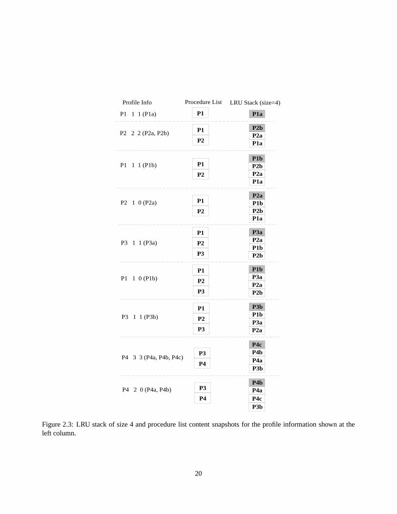
Profile Info LRU Stack (size=4)Procedure List

P1a

P2b P2a P1a

P1b P2b P2a P1a

P2a P1b P2b P1a

P3a P2a P1b P2b

P1b P3a P2a P2b

P3b P1b P3a P2a

P4c P4b P4a P3b

P4b P4a P4c P3b

P1

P1

P2

P1

P2

P1

P2

P1

P2

P3

P4

P3

P4

P1 1 1 (P1a)

P2 2 2 (P2a, P2b)

P1 1 1 (P1b)

P2 1 0 (P2a)

P3 1 1 (P3a)

P1 1 0 (P1b)

P3 1 1 (P3b)

P4 3 3 (P4a, P4b, P4c)

P4 2 0 (P4a, P4b)

P3

P1

P2

P3

P1

P2

P3

Figure 2.3: LRU stack of size 4 and procedure list content snapshots for the profile information shown at theleft column.

20

and the estimated worst case number of misses ismin(l1 � gl1;SP2P1) = min(1 � 1; 2) = 0. When procedureP2 is activated a 2nd time,SP1P2 = 1 because only one cache line of procedureP1 was activated since the

last occurrence ofP2. Thus the algorithm will increment theP2 � P1 edge weight bymin(l2 � gl2;SP1P2) =min(1 � 0; 1) = 1. ProcedureP3 is activated next, so bothP3 � P2 andP3 � P1 CMG edge weights will be

incremented bymin(l3 � gl3;SP2P3) = min(1 � 1; 2) = 0 and bymin(l3 � gl3;SP1P3) = min(1 � 1; 1) = 0,

respectively. Notice thatSP2P3 = 2 becauseP2a andP2b cache lines are still live while

SP1P3 = 1, because there

is only one live cache lineP1b from P1. Cache lineP1a has been replaced from the LRU stack.

When procedureP1 is reactivated, bothP3 � P1 andP2 � P1 edge weights are incremented bymin(l1 �gl1;SP3P1) = min(1�0; 1) = 1 andmin(l1�gl1;SP2P1) = min(1�0; 1) = 1, respectively. Notice that although

procedureP2 has two live cache lines (i.e.,P2a andP2b), only one is considered for the edge weight (P2a) since

it is the only one activated byP2 (the 4th trace entry) during the time window of the current and last appearance

of P1 (the 6th and 3rd trace entries, respectively). The subsequent P3 activation increments only theP3 � P1edge weight bymin(l3 � gl3;SP1P3) = min(1� 1; 1) = 0, because procedureP2 has not been activated during

the time span between the last two activations for procedureP3. Following procedureP3, the first appearance

of procedureP4 increments only theP4 � P3 edge weight bymin(l4 � gl4;SP3P4) = min(3� 3; 1) = 0, since

proceduresP2 andP1 currently do not have any live cache lines. Finally, at the next occurrence of procedureP4, we do not update the edge weight forP4�P3 since procedureP3 was not activated since the last activation

of procedureP4.The CMG captures procedure interaction beyond the caller-callee limit. Procedures may interact even

when they lie on either the same, or different, call chain(s). In addition, since the liveness of code is used to

record this interaction, temporal proximity of procedure invocations is the critical parameter that determines

the degree of procedure interference. To contrast the differences between a CG, TRG and a CMG, we develop

new characterization streams based on the Inter-ReferenceGap (IRG) model [91].

2.2.1 Procedure-based Inter-Reference Gap Modeling

There has been a significant amount of prior work on modeling the interaction and locality of code segments,

with most of them focusing on page [92, 93, 94] and/or cache line [95, 96, 97] locality and liveness.

In [96], Quong presents an estimation model that predicts miss rates for caches of arbitrary associativity

using profile information. This model requires a compressedform of the trace in order to approximate the

cache miss ratio, thus allowing trace compaction. Moreover, the model quantitatively measures the expected

cache interference between basic blocks by providing miss count estimates. He defines agapG as the interval

between successive references to a blockb. The gap ends with the current reference tob. The size of G is defined

as the number of unique addresses references occurring during G, and since the block ordering is preserved, its

21

contents are very similar to those of the LRU stack used for the CMG. Consider the gap G shown below:

... b b1 b2 b1 b3 b4 b2 b ...

in which b1; b2; b3; b4 are the unique blocks referenced inside G. Assume that everyblock bi occupiessicache lines. Whenb is referenced again, each address ofb has a(1�si �x) chance of surviving a conflict withbiblock. x is defined as the probability that two different addresses will collide. If X is a random variable, equal

to the number of cache lines, occupied byb, that are replaced during G, then the expected number of conflict

misses forb is: E[X] = s � [1�Xbi2G(1� x � si)] (2.1)

If a block bi appears more than once in G, it is considered only once in (2.1) since no more misses betweenb andbi can occur. By summing all the expected values for all the gapsin the trace, we get the miss count

estimate proposed in [96]. By exempting all pairs of blocks in (2.1) that belong to the same procedure, we take

into account the fact that most blocks of the same procedure do not collide in cache (assuming the procedure

fits in the cache). This last assumption is also taken into account in our CMG model, because we do not create

CMG self-edges. Since we want to estimate the number of misses between two different basic blocks,b; bi for

the current gap G, (2.1) becomes: E[X] = s � [1� (1� x � si)] (2.2)

The total number of estimated misses betweenb and bi is the sum over all gaps G of both blocks found in

the trace. The CMG model has several similarities and differences with the gap model. First, both models

function independent of any address mapping. For example, the size of a basic block is determined as the

average number of cache lines it occupies over all starting positions. Second, both models assume that a block

has equal probability of mapping to each cache line. Also, all cache misses are uniformly modeled based on

the LRU stack depth of each block reference. The only exception is cold-start misses. These are not handled

differently in the gap model but are excluded from the CMG edge weight.

In the CMG we measure procedure interference in the cache by looking at the cache lines of live procedures.

In other words, we record potential misses between blocks that do not belong to the same procedure, as is the

case with the gap model. As a consequence, each trace entry isnot a basic block, but a procedure chunkpi,consisting ofsi cache lines. If we replacebi with pi, we can derive a new formula, similar in spirit to (2.2).

Notice that the gap definition changes in the CMG. A gap, G0 in a CMG, is equivalent to a gap G (as described

in [96]), but only if the size of G is smaller or equal to the cache sizeL. Otherwise, G0 includes all past block

references whose total size is equal to the cache size, starting fromb. This is done to account for the finite-cache

effect. G = fb; bi; bj ; bi; bk; : : : ; bl; bg22

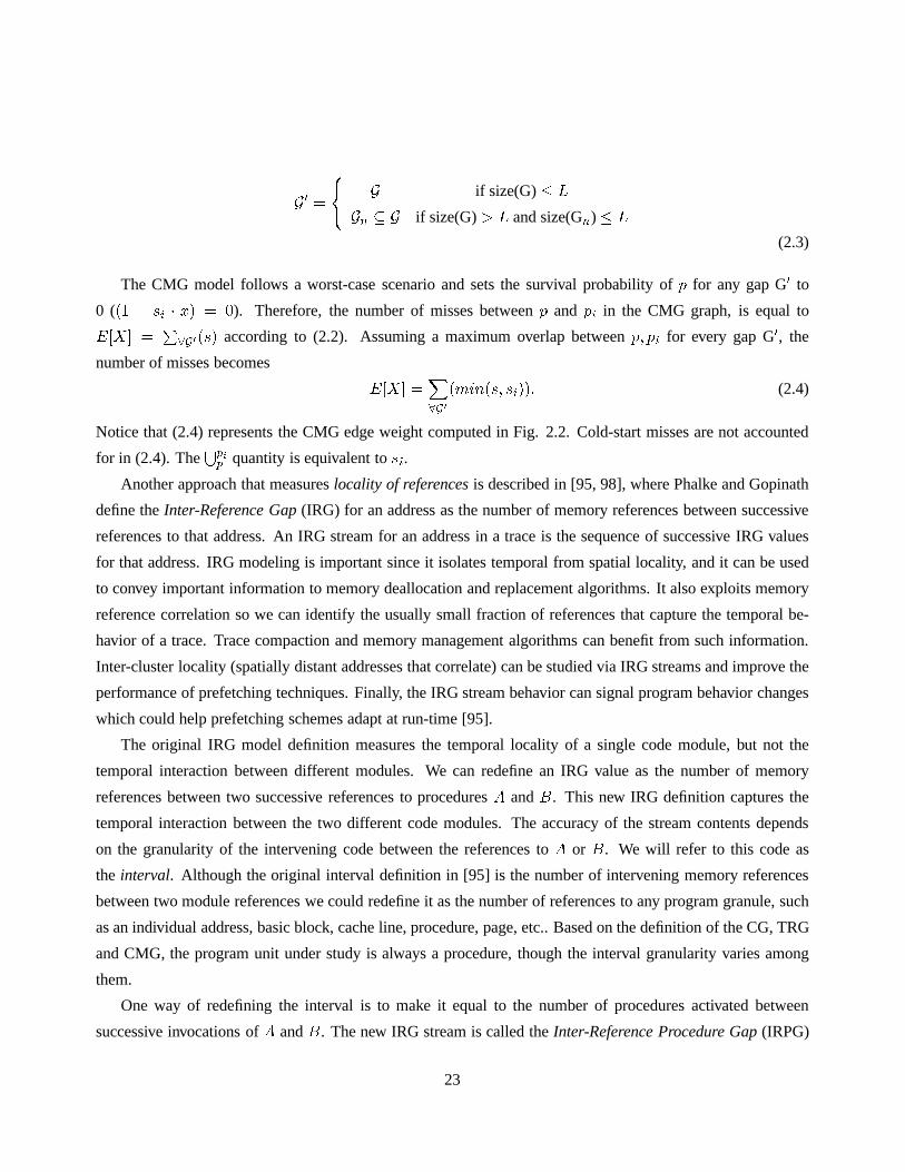
G0 = 8<: G if size(G)� LGn � G if size(G)> L and size(Gn) � L(2.3)

The CMG model follows a worst-case scenario and sets the survival probability of p for any gap G0 to

0 ((1 � si � x) = 0). Therefore, the number of misses betweenp and pi in the CMG graph, is equal toE[X] = P8G0(s) according to (2.2). Assuming a maximum overlap betweenp; pi for every gap G0, the

number of misses becomes E[X] =X8G0(min(s; si)): (2.4)

Notice that (2.4) represents the CMG edge weight computed inFig. 2.2. Cold-start misses are not accounted

for in (2.4). TheSpip quantity is equivalent tosi.

Another approach that measureslocality of referencesis described in [95, 98], where Phalke and Gopinath

define theInter-Reference Gap(IRG) for an address as the number of memory references between successive

references to that address. An IRG stream for an address in a trace is the sequence of successive IRG values

for that address. IRG modeling is important since it isolates temporal from spatial locality, and it can be used

to convey important information to memory deallocation andreplacement algorithms. It also exploits memory

reference correlation so we can identify the usually small fraction of references that capture the temporal be-

havior of a trace. Trace compaction and memory management algorithms can benefit from such information.

Inter-cluster locality (spatially distant addresses thatcorrelate) can be studied via IRG streams and improve the

performance of prefetching techniques. Finally, the IRG stream behavior can signal program behavior changes

which could help prefetching schemes adapt at run-time [95].

The original IRG model definition measures the temporal locality of a single code module, but not the

temporal interaction between different modules. We can redefine an IRG value as the number of memory

references between two successive references to procedures A andB. This new IRG definition captures the

temporal interaction between the two different code modules. The accuracy of the stream contents depends

on the granularity of the intervening code between the references toA or B. We will refer to this code as

the interval. Although the original interval definition in [95] is the number of intervening memory references

between two module references we could redefine it as the number of references to any program granule, such

as an individual address, basic block, cache line, procedure, page, etc.. Based on the definition of the CG, TRG

and CMG, the program unit under study is always a procedure, though the interval granularity varies among

them.

One way of redefining the interval is to make it equal to the number of procedures activated between

successive invocations ofA andB. The new IRG stream is called theInter-Reference Procedure Gap(IRPG)

23

in [91]. The CG graph records part of theIRPG stream by capturing all gaps of length 1. The IRPG stream

for proceduresA andB in the trace (A;C;D;C;B;A; F;E;A;B) is 3; 1; 1, assuming a value of 1 every timeA directly followsB (orB followsA).

In the TRG, every node represents a procedure and every edge is weighted by the number of times procedureA follows B and vice versa,only when both of them are found inside a moving time window. The window

includes previously invoked procedures, and its maximum size is equal to twice the L1 cache size [55, 99].

Once a procedure is activated, the window size is increased by the total number of cache lines that procedure

occupies. The window is organized as an LRU FIFO queue. Procedures are eliminated from the window once

the window size exceeds the upper limit. The IRG stream captured by the TRG redefines the interval between

two IRG values as the number of cache lines occupied by procedures activated between successiveA andBinvocations. We call this new IRG stream theInter-Reference Intermediate Line Gap(IRILG) [91]. The TRG

edge weight is simply the count (and not the sum) of all IRILG values that are less than the window size. The

TRG edge weights are more accurate than the CG weights because the IRILG stream is richer in content than

the IRPG (primarily due to the IRILG interval definition). The new interval definition takes into account the

number of cache lines instead of the number of procedures. Ina way, the IRILG values depend on both the

application calling behavior and the cache parameters, while the IRPG values depend only on the former. The

TRG edge weights also permit the recording of procedure interaction at a wider range than the CG.

The CMG edge weight between proceduresA andB is updated only whenA andB follow one another

inside a moving time window. The window is managed as an LRU FIFO queue. Every time a procedure is

activated only theuniqueactivated cache lines that belong to that procedure are inserted in the window. A

procedure is replaced only if the total number of cache linesin the window exceeds the window sizeand there

are no cache lines of that procedure in the window. The upper limit of the window is set to be equal to the

number of available cache lines in the L1 cache. In order to record the window contents for a CMG, we define

the Inter-Reference Active Line Set(IRALS) for a procedure pair as the sequence of the number of unique

live cache lines referenced between any successive occurrences ofA andB. A CMG edge weight is updated

whenever theIRALS value is less than the window size and bothA andB are live.

In both the TRG and the CMG, procedures interact as long as they are found inside the time window. A

CMG, however, replaces procedures in the time window based on the liveness of cache lines that belong to

eitherA orB [68], while a TRG manages replacement on an entire procedurebasis [55]. Also, the contents of

the window in the CMG are not defined based on the total size of aprocedure’s body as in the TRG but based

on the individual activated cache lines. In addition, the CMG edge weight betweenA andB is incremented by

the minimum of the unique live cache lines of the successive invocations ofA andB. The TRG simply counts

the number of timesA andB follow each other.

24

0 10 20 30 40 50 60 70 80 90 1000

20

40

60

80

100

120Relative positioning between TRG and CMG (ixx)

TRG graph

CM

G g

rap

h

0 10 20 30 40 50 60 70 80 90 1000

200

400

600

800

1000

1200Relative positioning between CG and TRG (ixx)

CG graph

TR

G g

rap

h

0 10 20 30 40 50 60 70 80 90 1000

200

400

600

800

1000

1200Relative positioning between CG and CMG (ixx)

CG graph

CM

G g

raph

Figure 2.4: Edge ordering comparison between the TRG and CMG(upper left corner plot), the CG and theTRG (upper right corner plot) and the CG with the CMG (centered plot). All graphs are generated with profileinformation extracted from the ixx benchmark.

25

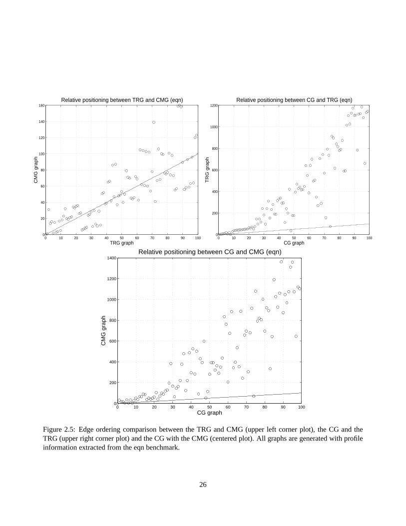
0 10 20 30 40 50 60 70 80 90 1000

20

40

60

80

100

120

140

160Relative positioning between TRG and CMG (eqn)

TRG graph

CM

G g

rap

h

0 10 20 30 40 50 60 70 80 90 1000

200

400

600

800

1000

1200Relative positioning between CG and TRG (eqn)

CG graph

TR

G g

rap

h

0 10 20 30 40 50 60 70 80 90 1000

200

400

600

800

1000

1200

1400Relative positioning between CG and CMG (eqn)

CG graph

CM

G g

raph

Figure 2.5: Edge ordering comparison between the TRG and CMG(upper left corner plot), the CG and theTRG (upper right corner plot) and the CG with the CMG (centered plot). All graphs are generated with profileinformation extracted from the eqn benchmark.

26

In order to compare the contents of the three graphs, we sorted the edge lists for all graphs in decreasing

weight order and plotted the relative positioning of the first 100 edges of one graph against another. Figs.

2.4 and 2.5 show the relative positions for eqn and ixx. We provide 3 plots per benchmark. Each plot shows

the relative edge ordering between two graphs (G1, G2). A mark at location (i; j) means that the edge under

consideration was foundith in theG1 graph’s ordered edge list andjth in theG2 graph’s ordered edge list.

Points on the straight line correspond to edges with the samerelative position in both edge lists. Points lying

above (below) the straight line indicate edges with a higherpriority in theG1 (G2) edge list. The figures

compare the ordering of the first 100 CG edges with the TRG and CMG edge list and the ordering of the first

100 TRG edges with the CMG edge list.

As we can observe, the contents of the CG are significantly different than those of the TRG or the CMG.

More specifically, both the CMG and the TRG promote other procedure pairs in the edge list. Those are either

found to have lower significance (edge weight) in the CG, or they are not recorded at all because they simply do

not exhibit the caller-callee relationship. The TRG and CMGcontents though are found to be similar since most

points tend to lie around the straight line. This is expectedsince both graphs investigate temporal procedure

interaction at a wider range than the CG. Differences are dueto the way procedure liveness and edge weights

are computed.

If we look at the computational complexity of building thesegraphs, the CG is the fastest one to construct. Ifn is the number of trace entries, the CG simply needs one pass ofthe entire trace. For every pair of consecutive

trace entries, we compare the procedure ids. If the ids are different we increment the edge weight between

the two procedures. The algorithm has a running time ofn and a complexity ofO(n). A single pass is also

required when building the TRG. For every trace entry we search a list of previously executed procedures. If

the currently invoked procedure,p, is found in the list we update the TRG edges betweenp and the procedures

in the list starting based on the TRG algorithm. If the procedure is not in the list we append it and properly

update the list to keep the size of its procedures equal to twice the cache size. Although the number of list

entries is not fixed, the maximum number of procedures can bec wherec is the number of cache sets in the

instruction cache under consideration. Since we need two passes over the list the running time is2 � c � n and

the complexity becomesO(n).The CMG also requires a single pass over the trace. For each trace entry we need to first search an array of

lists for every activated cache set ofp. Theoretically, the maximum number of activated cache setsis equal to

the procedure size divided by the cache set size. However, wekeep information only for the cache sets of the

instruction cache. Therefore, the maximum number of iterations isc. In reality, this is never the case because

each trace entry corresponds to a basic block. Only one cacheset is activated for the vast majority of trace

entries. Each entry of the array of lists points to a list of procedures that have accessed that cache set. We

27

maintain this data structure in order to keep track of globally unique accessed cache sets. The maximum size

of each procedure list can grow as large asap whereap is the number of active procedure in the profile. This

phase takes a total ofap � c steps although in reality a very accurate approximation isap.

We also need to search the procedure list for a match. The maximum size of the procedure list isc. If the

procedure is live we iterate over all cache sets accessed by the current procedure invocation in order to update

the LRU list and certain other data structures. As we mentioned above this number is approximately 1. In

addition, we need to adjust the size of the LRU list so that it is always equal or less than the instruction cache

size. The live procedure list must also be updated. Either ofthose steps requires a maximum ofc steps. The

final step consists of a single pass over all live procedures in order to update the CMG edge weights between

the procedure pairs that qualify. The maximum number of iterations is againc. On each iteration we need to

update a square bit matrix which keeps the number of unique cache sets accessed between any two activated

procedures. Although each size of the bit matrix has a lengthequal to the number of activated procedures in the

trace, we only iterate over the number of activated cache sets of the currently invoked procedure. Again, this

number is approximately constant. The total running time becomesn � (ap + 4 � c) which isO(n � ap) given

that the number of activated procedures is not bound. In practice,n� ap so the complexity becomesO(n).2.3 Pruning Algorithm

Both the CMG and the TRG generate a significantly larger number of edges compared to a CG. This is because

both graphs look for procedure interference inside a largertime window than a CG does. However, only a

small percentage of these edges carry important information. This section describes the pruning algorithm we

employed in order to concentrate on the highly interacting procedure pairs. Pruning also reduces the running

time of the placement algorithm since fewer edges have to be considered. Finally, cutting edges from the

original graph creates a pool of procedures that can fill gapsleft in the memory space after procedure placement.

To prune the graph, we select a threshold value by first sorting the edge weights in descending order, and

then starting at the heaviest edge, sum the edge weights until their sum is equal to or greater than 80% of

the total sum of all edge weights. The value of the last edge added becomes the threshold value. Every edge

weighing less than the threshold value is cut. The pruning step reduces the CMG into (usually) one strongly

connected subgraph that includes all heavily interacting procedures.

This threshold calculation is different from the adaptive algorithm used in [52] which partitioned the CG

into subgraphs. The partitioned CG in [52] was mapped in the cache by independently placing each one of its

subgraphs in the instruction cache without any conflicts. The idea was to facilitate mapping by considering a

subgraph at a time. In our case, the CMG can not be effectivelypartitioned due to its high connectivity. Thus,

28

although the pruned CMG does not usually fit in the cache, the increased accuracy of its edge weights imply an

edge ordering that can avoid more conflict misses after the mapping.

After pruning is performed, any procedure that remains connected to any other procedure is called apopular

procedure. Any remaining edges are calledpopular edges. The procedures that have no incident edge after

pruning are calledunpopular. Theunvisited proceduresare those that do not appear in the program profile.

Table 2.1 contrasts several edge-related statistics for the three graph models, CG, TRG and the CMG. Columns

2-5 and 6-8 show the number of edges and popular edges respectively. Table 2.2 is associated with procedures.

Column 2 shows the total number of procedures in the program (the number in parentheses is the total number

of activated procedures during profiling) while columns 3-5list the average size in Kb of popular procedures

for each of the graphs. Columns 6-8 present the total number of popular procedures for each graph.

Program # edges # pop edgesCG TRG CMG CG TRG CMG

perl 155 2502 3499 18 115 127gcc 3122 547081 135738 315 25838 7229edg 3789 1057644 347519 127 10663 3862gs 2027 390259 141730 218 31038 13731troff 1642 139531 95242 72 4189 2301eqn 898 40121 37289 37 2086 1185ixx 712 14945 18980 42 883 819eon 179 9045 8478 52 2381 2158porky 1698 165025 77482 276 11689 9402bore 1607 155508 75699 237 11001 9533lcom 1642 147980 97800 25 508 467

Table 2.1: Edge-related statistics: number of edges for CG,TRG and CMG (columns 2-4) and number ofpopular edges for CG, TRG and CMG (columns 5-7).

It is clear from Table 2.1 that the CG captures code interference at a much smaller scale than either the TRG

or the CMG. On the average, the TRG creates a larger number of edges than the CMG since it defines a window

with a size double that of the CMG (twice the cache size). The difference between the CG and the CMG, TRG

popular edge sets is significant. The popular edges, and their associated procedures shown in columns 6-8 of

Table 2.2, define the application working set according to each graph model. The CG, as expected, defines the

smallest working set. Even in perl, where the popular procedure set among the three graphs is essentially the

same, the number of CG popular edges is significantly smaller. The CMG detects a noticeably smaller popular

procedure group than the TRG only in gcc, edg and eqn. In all other benchmarks, the set is approximately the

29

same in size. Their intersection (not shown here), showed that a majority of the popular procedures is found in

both sets.

Program # procs pop procsKb Kb Kb # # #

total (active) CG TRG CMG CG TRG CMGperl 671 (91) 2.50 2.41 2.22 20 21 23gcc 2328 (1056) 1.54 1.09 1.27 254 657 481edg 3486 (1512) 0.92 0.82 0.82 106 358 138gs 4400 (1198) 0.48 0.38 0.37 199 380 415troff 1818 (703) 0.54 0.35 0.38 71 201 182eqn 850 (387) 0.82 0.43 0.53 41 145 99ixx 1581 (294) 1.21 0.66 0.65 36 82 87eon 2763 (135) 0.27 0.24 0.28 55 89 90porky 3478 (575) 0.32 0.43 0.42 175 296 290bore 2471 (559) 0.40 0.42 0.43 171 299 308lcom 1527 (692) 0.22 0.87 0.92 30 43 40

Table 2.2: Procedure-related statistics: static procedure count (column 2), number of activated procedures(column 2 in parenthesis), average static popular procedure size in Kb for CG, TRG and CMG (columns 3-5)and number of popular procedures for CG, TRG and CMG (columns6-8).

2.4 Cache-Sensitive Procedure Reordering Algorithm

After pruning, the next step is to map the popular proceduresin the cache address space so that potential

conflicts between them are minimized. To map procedures, we employ a cache line coloring algorithm, similar

to the one originally proposed in [52]. We modified the algorithm in [52] so that a proper mapping could be

enforced for caches of arbitrary organization (the algorithm in [52] was proposed for direct-mapped caches,

although an extension for associative caches was suggested).

In order to properly define cache conflicts for caches of arbitrary associativity, size and line size, we changed

the view of the cache address space from the one traditionally used in [52] and [55]. We define the cache address

space as the group of cache sets for a specific cache organization. A color is equivalent to a cache set (and not a

cache line as it was the case in [52]). We will use the term cache set and cache color interchangeably throughout

the remainder of this chapter. A procedure is mapped (colored) in the cache as follows: first, it is partitioned

into cache lines and then it is assigned a starting cache set in the cache address space. If two procedures have

at least one cache line being mapped to the same cache set, then they overlap. The degree of overlap (ovd)

30

for a given cache set and set of procedures, is equal to the number of cache lines of all the procedures that are

being mapped onto that same cache set. The maximum degree of overlap is defined as the maximum value ofovd for all cache sets in the cache address space. If the maximum degree of overlap for a set of procedures

(over all cache sets in a given cache) is greater than the degree of associativity of that cacheca, then there exist

potential conflicts between those procedures. Thus, we mustrelocate at leastovd � ca procedures in order to

fully eliminate conflicts for this set of procedures. Note that if the test between the degree of overlap and that

of associativity fails, conflicts will occur, independent of the replacement policy used in the cache (we assume

that all instruction accesses are allocated in the instruction cache and no bypassing is employed).

P1 P1 P1P2 P2

P3 P3P2

1 1 2 1 1 0 0 0 1 1 0 0

2-way set associative cache cache address space : 12 cache sets

P1 P1P2 P2 P2

P3 P3

1 2 3 1 1 0 0 0 0 0 0 0

P1

degree of overlapping :

degree of overlapping :

cache address space

cache address space

P1, P2 size : 3 cache linesP3 size : 2 cache lines

Figure 2.6: Computing the degree of overlap between procedures in the cache address space.

Fig. 2.6 presents an example of how we computeovd. We assume a 2-way set associative cache, with a

total of 12 cache sets. Initially, proceduresp1; p2 andp3 are mapped in such a way so that the maximumovdis equal to 3. Sinceovd > ca = 2, conflicts can occur in the shaded cache area of the cache address space.

By moving one of the three procedures (p3 in Fig. 2.6), we can decrease the maximumovd to 2 and avoid any

conflicts between the three procedures. Notice that this approach works for any cache size, line size, or degree

of associativity.

A direct consequence of altering the cache address space concept is a modification on the definition of

the unavailable set for a given procedure. In [52], the unavailable set for a procedurep was defined as the

cache lines occupied byp’s parents and children in the CG which have already been mapped. We redefine

the unavailable set as the range of cache sets occupied byp’s neighbors in the CMG which have already been

mapped, and for which there exist conflicts in the cache address space. The main body of the coloring algorithm

consists of a loop, iterating over all popular edges in descending edge weight order. The pseudo-code is shown

31

in Fig. 2.7.

As the algorithm traverses the sorted popular edge list, four possible cases may be encountered (see Fig.

2.7):� Case I : Proceduressrc anddst are not mapped. In this case we place them sequentially in thecache

address space, the larger procedure first. Sequential placement guarantees that the number of conflicting

colors between the two procedures are minimized. If both of them fit in the cache, then conflicts are

eliminated. The two procedures form a compound node. A global index pointer is advanced by the

compound node size to allow the next pair of procedures to be placed in different colors in the cache

address space.� Case II : Both proceduressrc are mapped, but to different compound nodes,Cdst andCsrc. In this case,

we merge the compound nodes together, concatenating the smaller (e.g.Csrc), 3 to the larger, (e.g.Cdst).The side ofCdst, whereCsrc will be placed, is the one with the shortest distance fromdst to either end

of Cdst. After placing the small compound node, we check for color conflicts betweensrc anddst. If

conflicts still occur, we move the small compound node away from the large one in an attempt to find a

conflict-free mapping. If this is not possible, we restore the original mapping, leaving the small procedure

adjacent to the large one. After the placement search is complete, we update the colors for all procedures

in the small compound nodes and merge the two nodes.� Case III : Only one of the procedures is mapped. Suppose that proceduresrc is mapped anddst is not.

In this case, we mergedst intoCsrc by placing it on the end ofCsrc, which is the shortest distance from

thesrc from either side ofCsrc. This heuristic is selected because the probability of being able to mapdst with no conflicts is increased, as the distance betweensrc anddst is reduced. After placingdst, we

check for color conflicts betweendst andsrc. If there are conflicts, we insert space between one end ofCsrc anddst until the mapping is conflict free. If a conflict free mapping is not possible, we restore the

original mapping wheredst was adjacent toCsrc.� Case IV : If both procedures are mapped and belong to the same compound node, we first check for color

conflicts betweensrc anddst. If there exist conflicts, we move the procedure closest to either end of the

compound node (e.g.,src) to the side of the node, creating a space or gap. We then checkagain for color

conflicts betweensrc and its unavailable set. If conflicts exist, we movesrc further away from the node

to eliminate those conflicts. If conflicts are inevitable, the original location inside the compound node is

used.3The compound node size is measured in total number of cache lines occupied by its procedure-members.

32

Input: list of popular edges ledge,Sort ledge on decreasing weight order; l1 color = 0;foreach e in ledgesrc = source(e), dst = destination(e);

if (src 6= mapped and dst 6= mapped) /* Case I */Form a compound node by placing the smaller procedure after the larger in L1 cache;Assign l1 color to the large and l1 size(large) mod L1 CACHE SETS to the small procedure;l1 color += (l1 size(src) + l1 size(dst)) mod L1 CACHE SETS;

elseif ((src == mapped) and (dst == mapped) and (Csrc 6= Cdst)) /* Case II */select p = dst or src based on minimum size of their compound node;Place small compound node on the left side of the large one;if (color conflicts(src; dst) exist)

move small compound node so that src is next to dst;if (color conflicts(src; dst) exist)

restore previous mapping;endif

endifmerge Csrc with Cdst;

elseif (only one procedure is mapped (e.g. src)) /* Case III */Place dst on the side of Csrc so that distance between src and dst is minimized;if (color conflicts(src; dst) exist)

place dst next to src;if (color conflicts(src; dst) exist)

restore previous mapping;endif

endifincorporate dst into Csrc;adjust compound node size if gap is required;

elseif ((src == mapped) and (dst == mapped) and (Csrc == Cdst)) /* Case IV */if (color conflicts(src; dst) exist)

select p = dst or src based on their minimum distance from either side of the compound node;place p, on that side;if (color conflicts(p,neighbors(p)) exist)

compute unavailable set(p) and find minimum area to place p with no conflicts;if (area does not exist)

restore original mapping for p;endif

endifendifadjust compound node size if gap is required;

endifendfor

Figure 2.7: Single-level cache line coloring algorithm.

33

A more elaborate discussion and an analytical example on theprocedure cache coloring algorithm can be

found in [52]. Table 2.3 shows the number of times each case isencountered in our benchmark suite when

no basic block reordering is applied. If basic block reordering is permitted, then the procedure sizes that need

to be colored change and so do the statistics in Table 2.3. Thenumbers in parentheses in column 5 represent

how many times two procedures from the same compound node hadcolor conflicts between them, given their

original relative position in the node. Notice that although most of the times two procedures are found in the

same compound node, no color conflicts are found and the next procedure pair is examined. The algorithm

spends most of its time attaching an unmapped procedure to a compound node (case 3). This trend is also

observed when basic block reordering is used before coloring.

2.4.1 Complexity Analysis

The first step of the procedure placement algorithm is to sortpopular edgespei in decreasing weight order.

That takespe � log pe steps. During the main loop of the algorithm we iterate over all popular edges. Cases

I is implemented in constant time. Cases II and III are more expensive than Case I, since they require a loop

over all L1 colors to compute theovd and check for conflicts. Furthermore, Case II needs to iterate over all

nodes of the compound node that is being repositioned,cnp, to adjust the L1 coloring of its member procedures

once the compound node’s new position has been finalized. A similar loop is necessary to merge the two

compound nodes. Case IV computes the available set for the procedure under consideration. It also finds a

best fit among all available cache regions for the candidate procedure. The first step requires iterating over all

mapped neighbors,np, of the procedure to find any non-conflicting spaces in the cache. We also need to iterate

over all cache colors of each neighbor to compute theovd for the entire set of neighbors. Let us call the total

number of cache colorscsets. Best fit is accomplished by sorting all non-conflicting contiguous regions in the

cache in increasing size order. This process requirescsets � log(csets) steps. Overall, the complexity of the

algorithm becomes: pe � (np+ cnp+ np � csets+ csets � log(csets)) (2.5)

Although csets can be large, it is a constant and does not depend on the application. On the other hand,pe; cnp andnp depend on the number of edges and procedures. In the worst case,pe = np2; np = cnp = p (pis the number of activated procedures), leading to a complexity in the order ofO(p3 + p2 log(p2)) = O(p3).Based on the experimental results of Tables 2.2 and 2.1,np is much smaller than the total number of activated

procedures. Also,cnp is smaller thanp because we form and merge compound nodes only at the beginning.

The algorithm very quickly converges to a state where a single large compound node has been formed. The only

subsequent changes are either add a new procedure or reshuffle its current members. In addition, the number

34

Program Case I Case II Case III Case IVperl (CMG) 4 1 15 107 (12)perl (TRG) 3 1 15 96 (12)perl (CG) 6 3 8 1 (0)gcc (CMG) 36 31 409 6753 (291)gcc (TRG) 63 58 531 25186 (953)gcc (CG) 54 41 146 74 (9)edg (CMG) 14 7 110 3731 (7)edg (TRG) 31 24 296 10312 (27)edg (CG) 27 21 52 27 (1)gs (CMG) 31 25 353 13322 (0)gs (TRG) 32 28 316 30662 (0)gs (CG) 40 25 119 34 (0)troff (CMG) 18 16 146 2121 (5)troff (TRG) 28 26 145 3990 (4)troff (CG) 21 13 29 9 (0)eqn (CMG) 12 9 75 1089 (27)eqn (TRG) 14 11 117 1944 (54)eqn (CG) 11 6 19 1 (1)ixx (CMG) 10 8 67 734 (22)ixx (TRG) 8 7 66 802 (12)ixx (CG) 9 4 18 11 (0)eon (CMG) 6 5 78 2069 (0)eon (TRG) 15 14 59 2293 (0)eon (CG) 13 6 29 4 (0)porky (CMG) 15 14 260 9113 (3)porky (TRG) 23 22 250 11394 (1)porky (CG) 23 21 129 103 (0)bore (CMG) 14 13 280 9226 (4)bore (TRG) 24 23 251 10703 (0)bore (CG) 24 18 123 72 (0)lcom (CMG) 7 3 26 431 (0)lcom (TRG) 8 4 27 469 (0)lcom (CG) 8 3 14 0 (0)

Table 2.3: Visiting frequency of each case in the single-level cache line coloring algorithm (columns 2-5). Thenumber in parentheses in column 5 represents the number of times two procedures of the same compound nodeneed to be recolored because of conflicts.

35

of edges,e, is significantly lower thanp2. This difference is even larger after pruning. Most importantly, the

step of computing the unavailable set and fitting candidate procedures inside the cache address space specified

by the set, is infrequently performed (column 5 in Table 2.3,number in parentheses).

2.5 Main Memory-based Procedure Placement Algorithm

After placing procedures in the cache address space the nextstep is to assign procedures to main memory

offsets. Notice that in the previous step we do not assign absolute memory addresses since we want to be able

to generate a relocatable memory map. The main memory placement algorithm first assigns a memory offset

to all procedures and then to every basic block inside a procedure’s body. The pseudo-code of the procedure

assignment algorithm is shown in Fig. 2.8.

As a first step, the algorithm distributes all popular procedures to slots, based on their assigned cache color.

Then we select a cache color, find a procedure assigned to the selected cache color, place that procedure in

memory and advance the pointer to the next available color. Initially we start with cache color 0. In case there

is no candidate assigned to the selected color, we proceed with the next sequential cache color. That way,

we guarantee the algorithm will complete, since the entire cache address space is scanned until an unmapped

procedure is found. If there exists more than one proceduresfor mapping, we select the one connected via

the heaviest CMG edge weight to the previously mapped procedure. This is done in order to allow procedures

with high temporal interaction to be placed close to each other in memory and to prevent the working set of

the application from increasing. If none of the candidates is connected via a CMG edge with the previously

mapped procedure, we select one by random.

As we map popular procedures, we record gaps created in memory. Suppose thatprev color andcolor are

the starting cache sets for two successively mapped procedures. The size of the gap between them, expressed

in L1 cache lines, is shown below:gap = 8<: color � prev color if color � prev colorL1 CACHE SETS � prev color + color if color < prev color (2.6)

After mapping a popular procedure, we sort the gaps in increasing size order, and all unpopular procedures

in decreasing size order. Placement of unpopular procedures takes place using a best fit algorithm so that the

empty space among popular procedures is minimized. We then perform the same task for any unactivated

procedures in case gaps remain. The remaining unmapped unpopular and unactivated procedures are appended

at the end of the executable.

Table 2.4 lists the total memory gap space in Kb remaining after code reordering for each graph model.

36

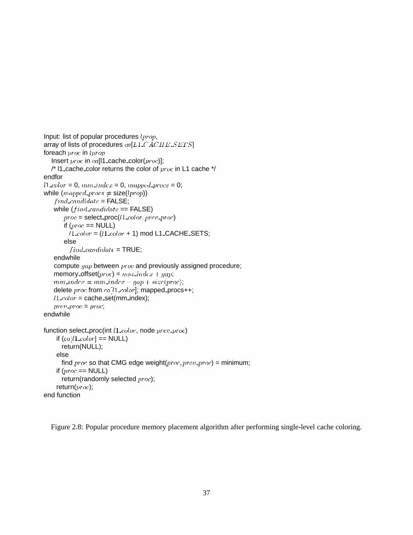
Input: list of popular procedures lprop,array of lists of procedures ca[L1 CACHE SETS]foreach proc in lprop

Insert proc in ca[l1 cache color(proc)];/* l1 cache color returns the color of proc in L1 cache */

endforl1 color = 0, mm index = 0, mapped procs = 0;while (mapped procs 6= size(lprop))find candidate = FALSE;

while (find candidate == FALSE)proc = select proc(l1 color; prev proc)if (proc == NULL)l1 color = (l1 color + 1) mod L1 CACHE SETS;elsefind candidate = TRUE;

endwhilecompute gap between proc and previously assigned procedure;memory offset(proc) = mm index+ gap;mm index = mm index+ gap+ size(proc);delete proc from ca[l1 color]; mapped procs++;l1 color = cache set(mm index);prev proc = proc;

endwhile

function select proc(int l1 color, node prev proc)if (ca[l1 color] == NULL)

return(NULL);else

find proc so that CMG edge weight(proc; prev proc) = minimum;if (proc == NULL)

return(randomly selected proc);return(proc);

end function

Figure 2.8: Popular procedure memory placement algorithm after performing single-level cache coloring.

37

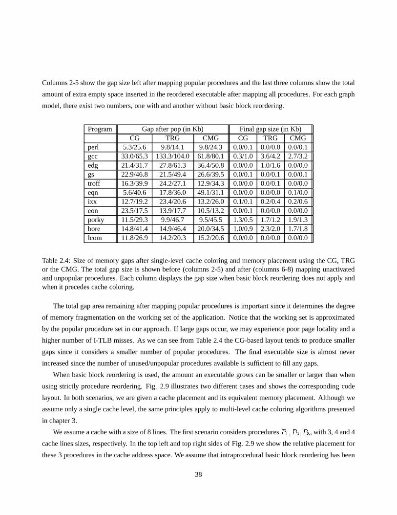
Columns 2-5 show the gap size left after mapping popular procedures and the last three columns show the total

amount of extra empty space inserted in the reordered executable after mapping all procedures. For each graph

model, there exist two numbers, one with and another withoutbasic block reordering.

Program Gap after pop (in Kb) Final gap size (in Kb)CG TRG CMG CG TRG CMG

perl 5.3/25.6 9.8/14.1 9.8/24.3 0.0/0.1 0.0/0.0 0.0/0.1gcc 33.0/65.3 133.3/104.0 61.8/80.1 0.3/1.0 3.6/4.2 2.7/3.2edg 21.4/31.7 27.8/61.3 36.4/50.8 0.0/0.0 1.0/1.6 0.0/0.0gs 22.9/46.8 21.5/49.4 26.6/39.5 0.0/0.1 0.0/0.1 0.0/0.1troff 16.3/39.9 24.2/27.1 12.9/34.3 0.0/0.0 0.0/0.1 0.0/0.0eqn 5.6/40.6 17.8/36.0 49.1/31.1 0.0/0.0 0.0/0.0 0.1/0.0ixx 12.7/19.2 23.4/20.6 13.2/26.0 0.1/0.1 0.2/0.4 0.2/0.6eon 23.5/17.5 13.9/17.7 10.5/13.2 0.0/0.1 0.0/0.0 0.0/0.0porky 11.5/29.3 9.9/46.7 9.5/45.5 1.3/0.5 1.7/1.2 1.9/1.3bore 14.8/41.4 14.9/46.4 20.0/34.5 1.0/0.9 2.3/2.0 1.7/1.8lcom 11.8/26.9 14.2/20.3 15.2/20.6 0.0/0.0 0.0/0.0 0.0/0.0

Table 2.4: Size of memory gaps after single-level cache coloring and memory placement using the CG, TRGor the CMG. The total gap size is shown before (columns 2-5) and after (columns 6-8) mapping unactivatedand unpopular procedures. Each column displays the gap sizewhen basic block reordering does not apply andwhen it precedes cache coloring.

The total gap area remaining after mapping popular procedures is important since it determines the degree

of memory fragmentation on the working set of the application. Notice that the working set is approximated

by the popular procedure set in our approach. If large gaps occur, we may experience poor page locality and a

higher number of I-TLB misses. As we can see from Table 2.4 theCG-based layout tends to produce smaller

gaps since it considers a smaller number of popular procedures. The final executable size is almost never

increased since the number of unused/unpopular proceduresavailable is sufficient to fill any gaps.

When basic block reordering is used, the amount an executable grows can be smaller or larger than when

using strictly procedure reordering. Fig. 2.9 illustratestwo different cases and shows the corresponding code

layout. In both scenarios, we are given a cache placement andits equivalent memory placement. Although we

assume only a single cache level, the same principles apply to multi-level cache coloring algorithms presented

in chapter 3.

We assume a cache with a size of 8 lines. The first scenario considers proceduresP1; P2; P3, with 3, 4 and 4

cache lines sizes, respectively. In the top left and top right sides of Fig. 2.9 we show the relative placement for

these 3 procedures in the cache address space. We assume thatintraprocedural basic block reordering has been

38

P1P2

P3

cache address space cache address space

P2P1 P1

P3 P3 P3P2 P2

P1 P2 P3P2P1 P1 P2 P2P3 P3 P3

P1 P1 P1 P2 P2 P2 P2 P3 P3 P3 P3

main memory address space

Gap Gap

P1 P1 P1 P2 P2 P2P2 P3P3P3 P3


P1

cache address space cache address space

P1 P1P2

P1 P1 P1P1 P1 P1 P1P2 P2 P2

P1 P1 P1 P1P2 P2 P2 P2 P2 P2 P2 P2 P2 P2 P2P2

P1 P1 P1 P2P2 P2 P2


P1 P1 P1 P1 P2 P2 P2 P2

Gap

P1 P1 P1 P2 P2P2P2


P1 P1 P1 P1 P2 P2 P2 P2

Gap

P2

Figure 2.9: Scenarios where code size can increase in the presence/absence of basic block reordering.

applied to them and all their frequently executed sequencesof basic blocks have been moved to the beginning

of their address space, forming the shaded area which we callHot Region(HR). The top left arrangement is

based on coloring the HR of each procedure, while the top right assumes a coloring of the entire procedure

body (no basic block reordering). The main memory layout lies below the cache layout. Although the HR

allows overlapping of the procedure bodies in the cache and leads to a more compact layout in the cache, it

creates gaps in main memory. When the HR is not considered in coloring, the purely sequential cache layout

shown in the top right of Fig. 2.9 leads to a memory layout withno gaps. This layout actually represents the

ideal case, but does occur in practice. The example illustrates a scenario where the code size is increased when

basic block reordering is employed.

In the second scenario, proceduresP1 andP2 are placed in the cache in two different ways. Again, in the

first approach, only the HRs are colored, while the second approach considers the entire procedure body. In

the later, we assume thatP2 is placed on the side of the compound node ofP1 leading to the layout of Fig.

2.9. The generated memory gap is larger when no basic block reordering is applied. In general, the gap size

depends on the HR size relative to the procedure size as well as to the relative placement in the cache between

39

two procedures.


The memory placement algorithm initially places popular procedures based on their assigned L1 cache color

into a one-dimensional array. Every array element points toa list of procedures mapped to the same color in

the cache. The assignment process takespp steps, wherepp is the number of popular procedures. The main

loop that assigns a starting memory address consists of two steps. During the first step we look for a procedure

to be mapped by performing a linear search over the array. Thesearch wraps around when the end of the array

is reached and ends either when it reaches its starting point, or when it detects an array element pointing to a

non-empty list. The first case indicates the end of the algorithm since all procedures have been mapped. In

the second case, we search the procedure list to find the procedure that is connected via the heaviest CMG

edge with the procedure that has just been mapped. Once a procedure is found, we compute its new memory

address, find out the gap size that may have been created and continue with the search for another procedure.

The new search starts from the end of the newly mapped procedure. Letl be the number of procedures in an

array element andcsets the number of available cache colors. The worst-case scenario is to have all popular

procedures mapped to a single location in the array (i.e.,l = pp). The first step will takecsets � pp time (each

time we will iterate over the entire array and we will search the entire list of popular procedures). Since we

need to map allpp procedures, the complexity of the algorithm becomesO(pp � (csets � pp)) = O(pp2), sincecsets is a constant. However, the distribution of procedures in the cache is much more uniform. Thus, we

seldom have to search a large part of the array to find non-empty elements. Also we rarely find thatll = pp.

The actual running time of the algorithm is close to linear, especially sincell tends to be independent ofpp.

2.6 Intraprocedural Basic Block Reordering Algorithm

This section describes an intraprocedural basic block reordering algorithm. In order to perform this task, we

record transition frequencies between activated basic blocks. The trace contents, as they are described in

section 2.2, provide this information. We then build a graph, called theDynamic Control Flow Graph(DCFG),

for every popular procedure. A DCFG is a directed graph, where every node represents a basic block, and

every edge is weighted by the number of transitions between two blocks. The number of edges recorded in the

DCFG depends on the number of transitions between basic blocks, as recorded in the profile. Hence, a DCFG

is always a subgraph of a procedure’s CFG (the relationship is similar to that between a DCG and a CG).

Notice that we count edge frequencies to record basic block interaction. We could have weighted the edges

using temporal information (based on the TRG or the CMG edge weight algorithm), or using path profiling

40

[100, 101]. Although there are cases where path profiling canbe more accurate than edge profiling [101], this

approach is out of the scope of this thesis. On the other hand,we did not compute CMG edges on a basic block

basis since a CMG graph captures interaction between units that are at least as large as a cache line (assuming

that the CMG would used to record interaction in a cache). Since most basic blocks are smaller than a cache

line, constructing another CMG on a basic block basis is not necessary.

Since the DCFG records intraprocedural basic block interaction, we take special care when basic blocks

transfer control flow outside procedure boundaries (usually via procedure calls). Whenever such a block is

found, we create an edge between that block and the block where the control flow returns after the call com-

pletes. The edge is weighted with the number of times the block making the call is executed. Finally, we do not

record transitions for short loops, where the source and thedestination is the same basic block.

After building the DCFGs for all popular procedures, we sortthe DCFG edges in decreasing weight order.

Then we reorder the blocks by forming compound nodes as we traverse the sorted list of edge weights. There

are four possible cases the algorithm encounters during thetraversal:� Case I : Both basic blocks are unmapped. In that case it forms anew compound node by placing the

source followed by the destination basic block.� Case II : The source block is mapped and the destination is unmapped. Then if the source lies on the tail

of its compound node, we append the destination to the end of the compound node (immediately after

the source). If this is not the case, we create a new compound node with the destination block as the only

member.� Case III : The destination block is mapped and the source is unmapped. If the destination is the head of its

associated compound node, we append the source to the beginning of the compound node (immediately

before the source). If this is not the case, we create a new compound node with the source block as the

only member.� Case IV: Both blocks are mapped, but belong to different compound nodes. If the source is the the tail

and the destination is the head of their compound nodes respectively, then we concatenate the blocks of

the two compound nodes by placing the the node of the source block before the node of the destination.

The two compound nodes are merged into a single node.

Fig. 2.10 illustrates the four different cases.

At the end of the reordering step there may be several compound nodes remaining. We traverse the sorted

edge list again and apply case IV in order to merge all the nodes together. The primary motivation, behind basic

block reordering, is to provide uninterrupted control flow.Hence, we move basic blocks to allow branches to

41

Case I

A B A B

Case II

A B

before after

...... A B......

afterbefore

A B...... ...... A B...... ......

Case III

A B ......

afterbefore

BA ...... ...... BA ...... ......

B

A

......A...... A B ............

Case IVafterbefore

B ......

Figure 2.10: Basic block placement decisions during intraprocedural basic block reordering.

fall through most of the time. In case a branch is not biased towards one of its possible targets, then we try

to position both targets (the fall through and taken targets) close to each other, in order to allow sequential (or

forward-based) prefetching to bring the taken target closer to the CPU. The algorithm is very similar to the one

proposed in [54]. All unactivated basic blocks are appendedafter the final compound node, in the order they

are found in the original executable.

Subsequently, we apply a partitioning algorithm that separates a procedure’s body into a hot and a cold

segment. No procedure splitting is performed. The procedure body remains intact, residing in a contiguous

address segment. However, we virtually bisect a procedure into two areas, the cold and hot region. The idea is

to use the hot segment as the effective procedure body that needs to be colored. The hot region needs to include

the most frequently accessed basic blocks (in the order specified by the basic block reordering step). The cold

region includes the rarely accessed and unactivated portions of a procedure’s body.

The partitioning step, as shown in Fig. 2.11, works as follows: we first compute the total sum of DCFG edge

weights. We define an upper bound that is equal to a fixed percentage of the total sum. We set this threshold to

42

90% for all the experiments in this thesis. We then sort all DCFG edges in decreasing weight order and traverse

the sorted list until the sum of the weights of the visited edges reaches the upper bound. The weight of the last

edge to be included in the sum computation is calledmin weight. The idea is to filter out the edges carrying the

least frequent transitions between blocks.

The next step is to determine the hot region of a procedure. This is done by iterating over all basic blocks

in the reordered basic block list. On each iteration we assign a basic block to the hot region if the block has

not been visited. We then mark the block as visited and check whether the next basic block will be examined

for inclusion in the hot region. We find the incoming and outgoing DCFG edges of the current basic block. We

compute the sum of edge weights for all incoming and outgoingedges that are above the edge threshold and

have not been visited before. This sum is computed over all basic blocks. The process of adding basic blocks to

the hot region stops either when all activated blocks have been visited or when the sum of edge weights exceeds

the upper bound.

The basic block reordering algorithm requires a code fix-up step, where unconditional branches are inserted

whenever needed to maintain correct program semantics. The5 different cases we implemented are shown in

Fig. 2.12.� Case I: The last instruction of a basic block is a conditionalbranch and the positions of the two target

blocks have been switched. In this case we need to replace thebranch with its dual to properly redirect

control flow.� Case II: The last instruction of a basic block is a conditional branch and the two target blocks have both

been moved away from the parent block. The solution is to keepthe same conditional branch opcode and

insert a new basic block, consisting of an unconditional branch which will redirect control flow to the

next sequential target block when the conditional branch falls through.� Case III: The last instruction of a basic block is a non-branch instruction and the target block has been

moved away from its parent. Fixing the code requires augmenting the parent block with an unconditional

branch that will transfer control flow to the target.� Case IV: The last instruction of a basic block is a procedure call (direct or indirect) and the return block

has been moved away from its parent. Again, we insert a new basic block consisting of an unconditional

branch, which points to the return basic block. The basic block is inserted right after the procedure call

instruction.� Case V: The last instruction of a basic block is an unconditional branch and the target block has been

appended to the end of the parent. In this case, we can delete the branch from the parent block. This is

43

upper bound = (P8e (weight(e))) � THRESHOLD; /* weight(e) returns the DCFG weight of edge e */ledge = Sort(list of DCFG edges) in decreasing weight order;e = first element(ledge); temp sum = 0;

while (temp sum � upper bound)temp sum += weight(e);min weight = weight(e);e = next(ledge; e); /* get next DCFG edge in sorted list */endwhilelbb = list of reordered basic blocks; hot region size = 0;foreach bb in lbb

if (bb has been activated)if (bb 6= visited)hot region size += size(bb);bb visited;endiflin = list of in-going edges of bb;foreach e in lin

if ((temp sum < upper bound) and (source(e) 6= visited) and (weight(e) > min weight))temp sum += weight(e);endif

endforlout = list of outgoing edges of bb;foreach e in lout

if ((temp sum < upper bound) and (destination(e) 6= visited) and (weight(e) > min weight))temp sum += weight(e);endif

endforif (temp sum � upper bound)

break;endif

endifendfor

Figure 2.11: Algorithm that virtually partitions a procedure into a hot and a cold region after applying intrapro-cedural basic block reordering.

44

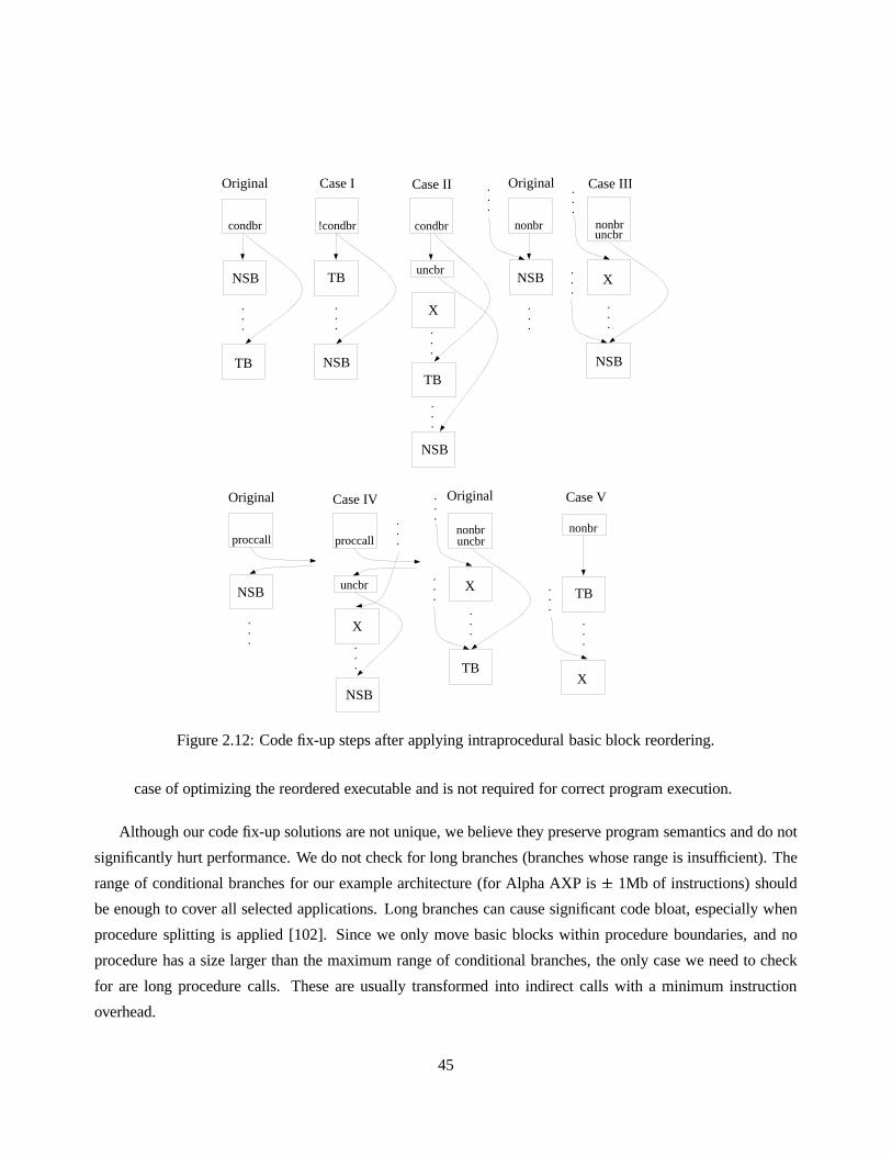
condbr

.

.

.

NSB

TB

Case I

!condbr

.

.

.

TB

NSB

Original Case II

condbr

.

.

.

TB

NSB

X...

uncbr

nonbr

.

.

.

NSB

Original...

Case III

nonbr

.

.

.

NSB

uncbr

X

.

.

.

.

.

.

proccall

.

.

.

NSB

Original Case IV

NSB

X...

uncbr

.

.

.proccall

.

.

.

TB

uncbr

X

.

.

.

.

.

.

Original Case V

.

.

.

TB

X

.

.

.

nonbr nonbr

Figure 2.12: Code fix-up steps after applying intraprocedural basic block reordering.

case of optimizing the reordered executable and is not required for correct program execution.

Although our code fix-up solutions are not unique, we believethey preserve program semantics and do not

significantly hurt performance. We do not check for long branches (branches whose range is insufficient). The

range of conditional branches for our example architecture(for Alpha AXP is� 1Mb of instructions) should

be enough to cover all selected applications. Long branchescan cause significant code bloat, especially when

procedure splitting is applied [102]. Since we only move basic blocks within procedure boundaries, and no

procedure has a size larger than the maximum range of conditional branches, the only case we need to check

for are long procedure calls. These are usually transformedinto indirect calls with a minimum instruction

overhead.

45

Program Extra UncBr UncBr-Del CBr-swi DCFG Pop proc HR size# # # bbs avg (Kb) total (Kb) avg (bytes)

perl (CMG) 118 (21) 27 102 20 2.24 8.8 392perl (TRG) 115 (20) 27 98 21 2.42 8.5 417perl (CG) 112 (20) 26 93 21 2.51 8.1 417gcc (CMG) 3511 (1463) 510 3578 39 1.30 345.7 736gcc (TRG) 4123 (1675) 603 4229 33 1.11 408.2 636gcc (CG) 2222 (1002) 307 2250 48 1.57 222.7 898edg(CMG) 1023 (330) 139 827 32 0.84 64.8 481edg(TRG) 2400 (666) 355 2254 28 0.85 169.0 483edg(CG) 937 (302) 119 741 37 0.95 55.3 535gs (CMG) 844 (195) 196 940 12 0.37 110.8 273gs (TRG) 796 (181) 190 872 12 0.38 102.4 276gs (CG) 595 (135) 150 612 17 0.49 69.1 356troff (CMG) 412 (103) 104 378 14 0.38 43.6 245troff (TRG) 418 (105) 109 382 13 0.36 45.4 231troff (CG) 209 (45) 43 193 17 0.55 20.1 290eqn (CMG) 260 (56) 50 227 16 0.54 30.6 317eqn (TRG) 299 (63) 58 264 14 0.44 39.3 277eqn (CG) 169 (46) 37 126 22 0.83 16.1 402ixx (CMG) 121 (34) 51 171 16 0.65 28.8 339ixx (TRG) 115 (32) 49 166 16 0.67 27.1 339ixx (CG) 90 (27) 38 126 24 1.22 18.2 517eon (CMG) 61 (7) 23 56 6 0.29 19.1 218eon (TRG) 58 (6) 23 54 6 0.24 18.8 216eon (CG) 48 (4) 20 46 8 0.27 13.0 242porky (CMG) 344 (40) 548 184 11 0.42 87.0 307porky (TRG) 351 (41) 577 188 11 0.43 89.6 310porky (CG) 159 (23) 272 103 9 0.31 41.0 240bore (CMG) 400 (50) 609 191 10 0.43 90.9 302bore (TRG) 378 (50) 586 183 10 0.42 86.2 295bore (CG) 226 (36) 324 127 10 0.40 48.5 290lcom (CMG) 160 (27) 55 75 20 0.93 15.2 389lcom (TRG) 164 (28) 58 78 20 0.88 15.8 376lcom (CG) 49 (9) 10 30 9 0.23 4.5 155

Table 2.5: Statistics associated with basic block repositioning: number of introduced unconditional branches(column 2) and subset of those which form a basic block (column 2, in parentheses), number of deleted un-conditional branches (column 3), number of conditional branches whose opcode has been switched (column4), average DCFG size in basic blocks (column 5), average DCFG size in Kbytes (column 6), total HR size inKbytes (column 7) and average HR size in bytes (column 8).

46

Table 2.5 lists statistics gathered after applying the basic block reordering algorithm on the popular proce-

dure set of each graph. The statistics vary between the graphs because the popular procedure sets are different.

Column 2 presents the total number of unconditional branches inserted, while the number of unconditional

branches inserted as independent basic blocks is listed in parentheses in the same column. Column 3 presents

the number of unconditional branches deleted as a side-effect of the reordering, and column 4 shows the number

of conditional branches whose opcode has switched. Column 5shows the average DCFG size in basic blocks,

while column 6 lists the average size of popular procedures in Kbytes. This average for the DCFG is computed

over popular procedures only. Note that the average popularprocedure size is slightly different from the one

shown in Table 2.2 because extra instructions have been inserted, and some instructions have been deleted as an

outcome of moving basic blocks. Columns 7 and 8 list the totaland average hot region (HR) size. The total size

of HR regions is a critical parameter because it approximates the working set of the application. Its relationship

to the L1 cache illustrates the degree of difficulty encountered by the cache coloring algorithm in achieving an

optimal solution, (i.e. a conflict free mapping for all HRs).Moreover, by comparing the numbers in columns

7 and 9, we can estimate the importance of basic block reordering. If the average popular procedure size is

comparable to the average HR size, then the main source of anypossible performance improvement should

come from procedure reordering.

2.7 Experimental Results

To evaluate the merit of our approach, we use a code reordering framework that can utilize as a base model any

of the three graphs described, CG, TRG and the CMG. The following six different configurations are simulated:� CMG-based procedure reordering (P sccmg)� CMG-based procedure and intra-procedural basic block reordering (Pbbsccmg)� TRG-based procedure reordering (P sctrg)� TRG-based procedure and intra-procedural basic block reordering (Pbbsctrg)� CG-based procedure reordering (P sccg )� CG-based procedure and intra-procedural basic block reordering (Pbbsccg)The sc superscript denotes that procedure reordering is performed for a memory hierarchy with asingle

cache level. For benchmarks that could be executed with SimpleScalar v3.0 [61], we provide cycle-based

results with and without code reordering. The modified code layout is simulated properly at all pipeline stages

47

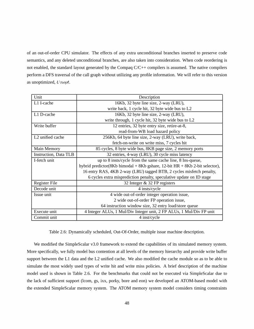
of an out-of-order CPU simulator. The effects of any extra unconditional branches inserted to preserve code

semantics, and any deleted unconditional branches, are also taken into consideration. When code reordering is

not enabled, the standard layout generated by the Compaq C/C++ compilers is assumed. The native compilers

perform a DFS traversal of the call graph without utilizing any profile information. We will refer to this version

as unoptimized,Unopt.Unit DescriptionL1 I-cache 16Kb, 32 byte line size, 2-way (LRU),

write back, 1 cycle hit, 32 byte wide bus to L2L1 D-cache 16Kb, 32 byte line size, 2-way (LRU),

write through, 1 cycle hit, 32 byte wide bus to L2Write buffer 12 entries, 32 byte entry size, retire-at-8,

read-from-WB load hazard policyL2 unified cache 256Kb, 64 byte line size, 2-way (LRU), write back,

fetch-on-write on write miss, 7 cycles hitMain Memory 85 cycles, 8 byte wide bus, 8KB page size, 2 memory portsInstruction, Data TLB 32 entries, 4-way (LRU), 30 cycle miss latencyI-fetch unit up to 8 insts/cycle from the same cache line, 8 Ins-queue,

hybrid predictor(8Kb bimodal + 8Kb gshare, 12-bit HR + 8Kb 2-bit selector),16 entry RAS, 4KB 2-way (LRU) tagged BTB, 2 cycles misfetch penalty,

6 cycles extra misprediction penalty, speculative update on ID stageRegister File 32 Integer & 32 FP registersDecode unit 4 insts/cycleIssue unit 4 wide out-of-order integer operation issue,

2 wide out-of-order FP operation issue,64 instruction window size, 32 entry load/store queue

Execute unit 4 Integer ALUs, 1 Mul/Div Integer unit, 2 FP ALUs, 1 Mul/Div FPunitCommit unit 4 inst/cycle

Table 2.6: Dynamically scheduled, Out-Of-Order, multipleissue machine description.

We modified the SimpleScalar v3.0 framework to extend the capabilities of its simulated memory system.

More specifically, we fully model bus contention at all levels of the memory hierarchy and provide write buffer

support between the L1 data and the L2 unified cache. We also modified the cache module so as to be able to

simulate the most widely used types of write hit and write miss policies. A brief description of the machine

model used is shown in Table 2.6. For the benchmarks that could not be executed via SimpleScalar due to

the lack of sufficient support (lcom, gs, ixx, porky, bore andeon) we developed an ATOM-based model with

the extended SimpleScalar memory system. The ATOM memory system model considers timing constraints

48

and models bus and cache line access contention. It also considers the side effects of code reordering (extra

branches being inserted/deleted), but it does not simulatethe effects of wrong path instructions.

In order to reduce the time needed for the simulations, we limited our simulations to a maximum of 300M

executed instructions for both SimpleScalar and the ATOM-based model. If an application required less than

300M instructions, we ran it to completion. Perl, gcc, edg, eon, porky and bore were profiled and tested using

300M instructions, starting at an offset of 50M instructions. All applications are compiled with the Compaq C

V5.2 and C++ V5.5 compilers, with full optimizations turnedon, on an Alpha-based 3000 AXP workstation

running Compaq Tru64 Unix v4.0.

IPC/MCPIProgram # of Instr. Unopt P sccmg P sctrg P sccg Pbbsccmg Pbbsctrg Pbbsccgperl 300M 1.25 1.28 1.44 1.49 1.45 1.55 1.55gcc 300M 1.02 0.99 0.97 0.98 1.15 1.11 1.11edg 350M 0.66 0.68 0.67 0.67 0.69 0.81 0.68troff 162M 1.59 1.78 1.81 1.74 1.91 1.92 1.77eqn 82.5M 1.93 1.65 2.00 1.99 2.05 2.05 1.97

gs 99.6M 1.43 1.43 1.43 1.42 1.40 1.41 1.41ixx 48.7M 1.53 1.64 1.58 1.47 1.43 1.43 1.45eon 300M 1.69 1.64 1.62 1.67 1.57 1.58 1.65porky 300M 1.70 1.68 1.69 1.68 1.66 1.66 1.69bore 300M 1.64 1.63 1.64 1.62 1.62 1.63 1.64lcom 32.2M 1.46 1.46 1.46 1.48 1.45 1.45 1.49

Table 2.7: Total number of executed instructions (column 2). Instructions per Cycle (IPC) for single cache levelcoloring code reordering configurations (columns 3-9, rows1-5). Memory Cycles per Instruction (MCPI) forsingle cache level coloring code reordering configurations(columns 3-9, rows 6-11).

Table 2.7 shows the IPC and MCPI for all single cache level coloring configurations. The IPC statistics

are generated with the SimpleScalar simulator. The higher the IPC, the better. MCPI is the average number of

Memory Cycles Per Instruction (MCPI). The lower the MCPI, the better. Procedure reordering improves the

IPC since it reduces the number of conflict misses in the L1 cache, therefore allowing more instructions to be

executed in a given number of cycles. It also reduces MCPI dueto the smaller number of misses in the L1

cache. In some cases, (e.g., eqn), performance drops. This is because the execution frequency of basic blocks

is not uniform across a procedure body. In addition, the frequently accessed paths are not contiguously laid

out. Basic block reordering solves these problems by placing all frequently activated chains of blocks at the

beginning of every procedure. In the absence of basic block reordering, large procedures will pose a problem.

49

The relative placement of smaller procedures may become worse and performance degrades. The original work

introducing the TRG [55] and the CMG [68] dealt with this problem indirectly. In the former, a second TRG

is built, this time for procedure chunks instead of procedure bodies. A chunk can be defined as a cache line

or a small set of cache lines. When placing procedures in the cache, the new TRG edge weights are used to

approximate the interaction of procedures at a finer level ofgranularity. The best respective placement of two

procedures is found iteratively, using a local optimal search.

In [68], we partition a procedure into cache lines, measure their respective execution frequencies and find

the largest group of frequently executed cache lines that are laid out contiguously in the procedure’s body. We

then use this group as the procedure’s effective body duringcoloring. When basic block reordering is employed,

the IPC is consistently increased across all graph models. Since procedures will occupy a smaller number of

colors, a better coloring can be found and the cache is betterutilized.

If we compare the 3 graph models, we can see that temporal codereordering using either the CMG or the

TRG can be beneficial. If the amount of work done between calls/returns is sufficient to replace from the I-cache

other procedures lying further away in the call chain, then the benefit of using the CMG or the TRG (instead of

the CG) is limited. This is the case with perl (see Fig. 2.13).On the other hand, edg requires interaction over

a wide temporal window to be recorded in order to improve performance. Recording accurate edge weights, as

in the CMG, is not of primary concern. Notice from Table 2.2 that the average popular procedure size is the

same for both the CMG and the TRG, although the CMG defines a much smaller set (138 compared to 358 of

the TRG). That, along with the small average procedure size (0.82Kb), indicates that it is beneficial to record

the interaction (perhaps with less accurate metrics) between more procedures instead of trying to focus on a

smaller procedure set by generating more accurate edge weights.

The TRG leads to the best performance improvement due to the larger scope of its temporal window (twice

the size of the target cache). This can also be verified by inspecting the number of popular procedures in Table

2.2 (358 for the TRG, 138 for the CMG and 106 for the CG), the number of popular edges in Table 2.1 (10665

for the TRG, 3862 for the CMG, 127 for the CG) and the total sizeof the popular procedure’s hot regions

in Table 2.5 (169Kb for the TRG, 65 Kb for the CMG and 55Kb for the CG). In gcc, the opposite scenario

occurs. The more accurate CMG edge weights produce a better code layout, although placement focuses on

a smaller popular procedure set (481 compared to 657 in TRG) with a higher average CMG procedure size

(1.27Kb compared to 1.09Kb in TRG).

Temporal-based code reordering may also degrade performance because it is more aggressive in capturing

and eliminating code interaction. When a CG is used, the edgeweights do not account for the procedure size.

Hence, if there exist several large procedures in the application, the CG-dependent edge ordering may give

priority to the interaction between small procedures over the interaction between large and small procedures.

50

The placement algorithm achieves a better placement for small procedures, especially since no prior placement

decisions are undone during coloring. When using either theTRG or the CMG, the interaction between large

and small procedures is assigned a higher priority than thatbetween small procedures. Then the coloring

algorithm tends to first place small procedures with respectto the large ones, leading sometimes to a worse

placement among small procedures compared to that of the CG (see ixx, bore, gs). This situation is detected

most often in a CMG, because of the accuracy represented in its edge weights which tend to magnify this

phenomenon (see eqn).

Fig. 2.13 and 2.14 show the performance improvement of different single cache coloring configurations

over the baseline. Our comparison metric is the ratio of the total number of cycles for the optimized case

over the standard layout. Fig. 2.13 corresponds to the SimpleScalar results and Fig. 2.14 to the ATOM-based

experiments. The ATOM-based results include only the cycles to satisfy memory requests. A positive ratio

implies improvement. Code reordering reduces the number ofexecution cycles by more than 15% in some

cases. Besides improving the cache hit ratio, performance also improves due to a lower BTB miss ratio and

reduced misfetch penalty (less branches are taken and less targets are stored in the BTB).

In the absence of basic block reordering, performance may degrade for the same reasons explained above.

It is interesting to notice that in two cases (gs and lcom), the CG-guided configuration failed to improve perfor-

mance with basic block reordering. This is because the CG does not always capture all the heavily interacting

procedure pairs. The CMG/TRG are more aggressive in definingthe popular procedure set. The CG is by

definition more conservative due to its limited range when recording code interaction. Performance can also

degrade because highly interacting procedures are defined as unpopular, and no cache-conscious placement is

found for them in either L1 or L2 cache. For example, in lcom, performance degradation is more severe when

basic block reordering is applied than when it is omitted. This is despite the fact that the size of popular proce-

dure set after basic block reordering drops to 4.5Kb from 6.6Kb. The main reason behind this drop is that more

L2 cache misses occur when basic block reordering is applied, as it can be seen in Fig. 2.16 which is described

next.

Fig. 2.15 and 2.16 display the L1/L2 cache miss ratios for allsimulated configurations. The L2 cache miss

ratio is computed over all references serviced by the L2 cache only, and so L1 cache hits are not considered in

the denominator. The impact of reordering on L1 cache miss ratios is obvious. A higher number of L1 cache hits

means that the traffic to L2 is reduced. This can be verified by inspecting the number of L2 references provided

next to the L2 cache bars. The number of L1 references for the SimpleScalar experiments are shown since

speculative execution can increase the traffic to L1. In the case of strict procedure reordering, the difference

is negligible and it can either increase or reduce the trafficto L1. There are several reasons behind this. First,

when both procedures and basic blocks are moved, basic blocks are laid out to improve the sequentiality of code.

51

0 0.05 0.1 0.15 0.2 0.25

sc−cmg

sc−trg

sc−cg

sc−bb−cmg

sc−bb−trg

sc−bb−cg

Cycle reduction for perl

Performance improvement (%)−0.06 −0.04 −0.02 0 0.02 0.04 0.06 0.08 0.1 0.12 0.14

sc−cmg

sc−trg

sc−cg

sc−bb−cmg

sc−bb−trg

sc−bb−cg

Cycle reduction for gcc

Performance improvement (%)

0 0.02 0.04 0.06 0.08 0.1 0.12 0.14 0.16 0.18

sc−cmg

sc−trg

sc−cg

sc−bb−cmg

sc−bb−trg

sc−bb−cg

Cycle reduction for troff

Performance improvement (%)−0.2 −0.15 −0.1 −0.05 0 0.05 0.1 0.15

sc−cmg

sc−trg

sc−cg

sc−bb−cmg

sc−bb−trg

sc−bb−cg

Cycle reduction for eqn


0 0.05 0.1 0.15 0.2 0.25

sc−cmg

sc−trg

sc−cg

sc−bb−cmg

sc−bb−trg

sc−bb−cg

Cycle reduction for edg


Figure 2.13: Cycle count reduction/increase after applying single cache level code reordering to the defaultcode layout. All results are generated via execution-driven simulation.

52

−0.015 −0.01 −0.005 0 0.005 0.01 0.015 0.02 0.025

sc−cmg

sc−trg

sc−cg

sc−bb−cmg

sc−bb−trg

sc−bb−cg

Memory cycle reduction for gs

Performance improvement (%)−0.08 −0.06 −0.04 −0.02 0 0.02 0.04 0.06 0.08

sc−cmg

sc−trg

sc−cg

sc−bb−cmg

sc−bb−trg

sc−bb−cg

Memory cycle reduction for ixx


0 0.01 0.02 0.03 0.04 0.05 0.06 0.07 0.08

sc−cmg

sc−trg

sc−cg

sc−bb−cmg

sc−bb−trg

sc−bb−cg

Memory cycle reduction for eon

Performance improvement (%)0 0.005 0.01 0.015 0.02 0.025 0.03

sc−cmg

sc−trg

sc−cg

sc−bb−cmg

sc−bb−trg

sc−bb−cg

Memory cycle reduction for porky


−2 0 2 4 6 8 10 12 14 16

x 10−3

sc−cmg

sc−trg

sc−cg

sc−bb−cmg

sc−bb−trg

sc−bb−cg

Memory cycle reduction for bore

Performance improvement (%)−0.025 −0.02 −0.015 −0.01 −0.005 0 0.005 0.01 0.015

sc−cmg

sc−trg

sc−cg

sc−bb−cmg

sc−bb−trg

sc−bb−cg

Memory cycle reduction for lcom


Figure 2.14: Memory cycle count reduction/increase after applying single cache level code reordering to thedefault code layout. All results are generated via trace-driven simulation.

53

0 5 10 15

unopt

sc−cmg

sc−trg

sc−cg

sc−bb−cmg

sc−bb−trg

sc−bb−cg

L1/L2 cache miss ratios for perl

L1 = 311.9ML2 = 8.6M

L1 = 311.5ML2 = 8.0M

L1 = 308.9ML2 = 5.0M

L1 = 308.1ML2 = 4.2M

L1 = 310.4ML2 = 4.4M

L1 = 309.0M L2 = 2.8M

L1 = 308.8M

L2 = 2.8M

percent (%)

L1L2

0 1 2 3 4 5 6 7

unopt

sc−cmg

sc−trg

sc−cg

sc−bb−cmg

sc−bb−trg

sc−bb−cg

L1/L2 cache miss ratios for gcc

L1 = 315.5ML2 = 8.9M

L1 = 316.5ML2 = 9.5M

L1 = 316.8ML2 = 9.9M

L1 = 316.6ML2 = 9.6M

L1 = 314.7M L2 = 6.4M

L1 = 315.2M

L2 = 7.2ML1 = 315.0M

L2 = 7.0M

percent (%)

L1L2

0 0.5 1 1.5 2 2.5

unopt

sc−cmg

sc−trg

sc−cg

sc−bb−cmg

sc−bb−trg

sc−bb−cg

L1/L2 cache miss ratios for troff

L1 = 163.7ML2 = 3.7M

L1 = 163.6ML2 = 2.3M

L1 = 163.5M

L2 = 2.1ML1 = 163.8M

L2 = 2.5M

L1 = 166.3ML2 = 1.7M

L1 = 165.4M L2 = 1.5M

L1 = 164.8M

L2 = 2.2M

percent (%)

L1L2

0 0.2 0.4 0.6 0.8 1 1.2 1.4 1.6 1.8 2

unopt

sc−cmg

sc−trg

sc−cg

sc−bb−cmg

sc−bb−trg

sc−bb−cg

L1/L2 cache miss ratios for eqn

L1 = 83.4ML2 = 755K

L1 = 83.1ML2 = 1.6M

L1 = 83.7ML2 = 624K

L1 = 83.8ML2 = 600K

L1 = 85.0ML2 = 436K

L1 = 84.8ML2 = 470K

L1 = 84.2ML2 = 652K

percent (%)

L1L2

0 2 4 6 8 10 12

unopt

sc−cmg

sc−trg

sc−cg

sc−bb−cmg

sc−bb−trg

sc−bb−cg

L1/L2 cache miss ratios for edg

L1 = 370.7M L2 = 19.1M

L1 = 371.1M L2 = 17.9M

L1 = 371.2M L2 = 18.2M

L1 = 371.1M L2 = 18.1M

L1 = 370.9M L2 = 17.0M

L1 = 368.9M L2 = 14.6M

L1 = 371.3M L2 = 17.3M

percent (%)

L1L2

Figure 2.15: L1/L2 cache miss ratios of both the optimized and the unoptimized executables. The number ofreferences to L1/L2 is appended on top of every bar. All results are generated via execution-driven simulation.

54

0 0.5 1 1.5 2 2.5 3 3.5

unopt

sc−cmg

sc−trg

sc−cg

sc−bb−cmg

sc−bb−trg

sc−bb−cg

L1/L2 cache miss ratios for gs

L2 = 1.0M

L2 = 1.0M

L2 = 1.1M

L2 = 1.0M

L2 = 842K

L2 = 820K

L2 = 889K

percent (%)

L1L2

0 2 4 6 8 10 12

unopt

sc−cmg

sc−trg

sc−cg

sc−bb−cmg

sc−bb−trg

sc−bb−cg

L1/L2 cache miss ratios for ixx

L2 = 810K

L2 = 1.47M

L2 = 1.09M

L2 = 418K

L2 = 180K

L2 = 177K

L2 = 258K

percent (%)

L1L2

0 0.5 1 1.5 2 2.5 3

unopt

sc−cmg

sc−trg

sc−cg

sc−bb−cmg

sc−bb−trg

sc−bb−cg

L1/L2 cache miss ratios for eon

L2 = 9.2M

L2 = 7.5M

L2 = 6.4M

L2 = 8.6M

L2 = 4.6M

L2 = 4.9M

L2 = 7.8M

percent (%)

L1L2

0 0.5 1 1.5 2 2.5 3

unopt

sc−cmg

sc−trg

sc−cg

sc−bb−cmg

sc−bb−trg

sc−bb−cg

L1/L2 cache miss ratios for porky

L2 = 8.6M

L2 = 8.4M

L2 = 9.0M

L2 = 8.5M

L2 = 7.4M

L2 = 7.2M

L2 = 8.3M

percent (%)

L1L2

0 0.5 1 1.5 2 2.5

unopt

sc−cmg

sc−trg

sc−cg

sc−bb−cmg

sc−bb−trg

sc−bb−cg

L1/L2 cache miss ratios for bore

L2 = 7.5M

L2 = 7.1M

L2 = 7.7M

L2 = 6.6M

L2 = 6.4M

L2 = 6.7M

L2 = 6.9M

percent (%)

L1L2

0 0.5 1 1.5 2 2.5 3 3.5 4 4.5

unopt

sc−cmg

sc−trg

sc−cg

sc−bb−cmg

sc−bb−trg

sc−bb−cg

L1/L2 cache miss ratios for lcom

L2 = 373K

L2 = 395K

L2 = 386K

L2 = 456K

L2 = 387K

L2 = 370K

L2 = 475K

percent (%)

L1L2

Figure 2.16: L1/L2 cache miss ratios of both the optimized and the unoptimized executables. The number ofreferences to L2 is also appended on top of every bar. All results are generated via trace-driven simulation.

55

The branch predictor will most of the time choose the next sequential address. The simulated fetch unit does

not store a target for a non-taken branch so aliasing in the BTB drops (fewer misfetches). Second, a number

of L1 accesses is eliminated because of unconditional branches that are deleted after basic block reordering,

though extra L1 accesses will be introduced by the unconditional branches that are added to preserve program

semantics. These branches can also put some pressure on the BTB, since they are always taken, and their targets

have to be fetched from the BTB to prevent bubbles in the pipeline.

I-TLB misses/Allocated pagesProgram Unopt P sccmg P sctrg P sccg Pbbsccmg Pbbsctrg Pbbsccgperl 24/2423 16/2412 18/2389 18/2389 14/2333 16/2302 16/2299gcc 1797/870 2469/871 2167/873 2130/870 1850/867 1295/869 1233/869edg 10532/651 6822/659 5906/661 11009/666 7063/661 3676/660 9777/665gs 91/302 70/264 79/283 71/265 70/264 79/281 80/284troff 53/181 39/167 39/167 38/166 36/164 37/165 35/163eqn 29/58 23/52 21/50 22/51 21/50 22/51 21/50

ixx 36/181 17/160 17/160 17/160 17/160 17/160 17/160eon 40/73 6/34 6/34 5/34 6/34 6/34 5/34porky 78/239 30/191 30/191 30/191 30/191 30/191 30/191bore 75/277 36/235 36/235 36/235 36/235 36/235 36/235lcom 43/202 25/175 25/175 25/175 25/175 25/175 25/175

Table 2.8: I-TLB misses and number of allocated pages for both the unoptimized case and the executablesoptimized with different configurations of single level cache code reordering.

Table 2.8 shows the number of I-TLB misses and the number of allocated pages for each application. The

number of I-TLB misses can increase after code reordering based on the final distribution of popular procedures

in the memory address space. Our results show that only in some cases (gcc), single cache coloring caused

more I-TLB misses. Even in gcc, the increase was substantialwhen procedure reordering was used alone. If

we observe Table 2.4, we see that the largest memory gaps werecreated for gcc. A solution to this problem

would be to adjust the memory placement algorithm to performsoftware-based page coloring [65]. Instead of

trying to place procedures as close to each other as possible, we could place them in pages that correspond to

different I-TLB entries. The remaining benchmarks show a significant decrease in I-TLB misses since popular

procedure mapping improved page placement. The number of allocated pages also decreases denoting that our

layout is both cache-conscious and page-sensitive.

Table 2.9 shows the number of instructions that were committed and those that were executed. The dif-

ference between the two occurs because our simulated machine employs speculative execution and certain

56

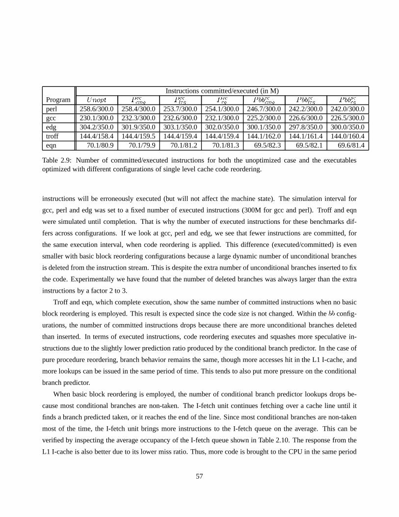
Instructions committed/executed (in M)Program Unopt P sccmg P sctrg P sccg Pbbsccmg Pbbsctrg Pbbsccgperl 258.6/300.0 258.4/300.0 253.7/300.0 254.1/300.0 246.7/300.0 242.2/300.0 242.0/300.0gcc 230.1/300.0 232.3/300.0 232.6/300.0 232.1/300.0 225.2/300.0 226.6/300.0 226.5/300.0edg 304.2/350.0 301.9/350.0 303.1/350.0 302.0/350.0 300.1/350.0 297.8/350.0 300.0/350.0troff 144.4/158.4 144.4/159.5 144.4/159.4 144.4/159.4 144.1/162.0 144.1/161.4 144.0/160.4eqn 70.1/80.9 70.1/79.9 70.1/81.2 70.1/81.3 69.5/82.3 69.5/82.1 69.6/81.4

Table 2.9: Number of committed/executed instructions for both the unoptimized case and the executablesoptimized with different configurations of single level cache code reordering.

instructions will be erroneously executed (but will not affect the machine state). The simulation interval for

gcc, perl and edg was set to a fixed number of executed instructions (300M for gcc and perl). Troff and eqn

were simulated until completion. That is why the number of executed instructions for these benchmarks dif-

fers across configurations. If we look at gcc, perl and edg, wesee that fewer instructions are committed, for

the same execution interval, when code reordering is applied. This difference (executed/committed) is even

smaller with basic block reordering configurations becausea large dynamic number of unconditional branches

is deleted from the instruction stream. This is despite the extra number of unconditional branches inserted to fix

the code. Experimentally we have found that the number of deleted branches was always larger than the extra

instructions by a factor 2 to 3.

Troff and eqn, which complete execution, show the same number of committed instructions when no basic

block reordering is employed. This result is expected sincethe code size is not changed. Within thebb config-

urations, the number of committed instructions drops because there are more unconditional branches deleted

than inserted. In terms of executed instructions, code reordering executes and squashes more speculative in-

structions due to the slightly lower prediction ratio produced by the conditional branch predictor. In the case of

pure procedure reordering, branch behavior remains the same, though more accesses hit in the L1 I-cache, and

more lookups can be issued in the same period of time. This tends to also put more pressure on the conditional

branch predictor.

When basic block reordering is employed, the number of conditional branch predictor lookups drops be-

cause most conditional branches are non-taken. The I-fetchunit continues fetching over a cache line until it

finds a branch predicted taken, or it reaches the end of the line. Since most conditional branches are non-taken

most of the time, the I-fetch unit brings more instructions to the I-fetch queue on the average. This can be

verified by inspecting the average occupancy of the I-fetch queue shown in Table 2.10. The response from the

L1 I-cache is also better due to its lower miss ratio. Thus, more code is brought to the CPU in the same period

57

of time. If the branch is mispredicted (misfetches are usually less of a problem due to lower aliasing in the

BTB), more instructions will be flushed from the pipeline on the average.

An additional issue we have to address is the difference between the number of L1 accesses and the number

of executed instructions. This occurs because not all wrongpath instructions execute before a misprediction is

detected. Some will still be waiting in the window buffer or in the I-fetch queue, and will be flushed from the

pipeline before entering the issue stage.

Average Ins window size/I-fetch queue size (in # of instructions)Program Unopt P sccmg P sctrg P sccg Pbbsccmg Pbbsctrg Pbbsccgperl 27.7/3.3 28.6/3.4 34.5/4.0 36.0/4.2 37.5/4.4 41.2/4.8 42.5/4.8gcc 22.2/2.6 21.5/2.5 20.9/2.4 21.3/2.5 26.6/3.1 25.2/3.0 25.4/3.0edg 13.3/1.4 14.2/1.5 13.8/1.5 14.1/1.5 15.1/1.6 17.9/2.0 14.6/1.6troff 22.3/2.9 27.6/3.6 27.7/3.6 26.2/3.5 31.2/4.1 32.6/4.3 29.2/3.9eqn 26.3/3.4 18.6/2.5 26.9/3.5 27.5/3.6 30.8/4.1 30.3/4.0 28.7/3.8

Table 2.10: Average Instruction window and Instruction fetch queue size for both the unoptimized case and theexecutables optimized with different configurations of single level cache code reordering.

Table 2.10 displays the average occupancy of the I-fetch queue and the centralized window buffer of the

processor. Both statistics are expressed in number of instructions. The I-fetch queue occupancy is listed to

highlight the effect of basic block reordering on the front-end of the processor. As we can see, whenever

overall performance improves, the average number of instructions found in the I-fetch queue increases. If strict

procedure reordering is employed, performance still improves because the average latency of fetching data from

the memory hierarchy drops. When we apply basic block reordering, the occupancy of the fetch unit increases

even more. Given the size of the queue (8 instructions), onlyperl, eqn and troff managed to fill at least half of

the fetch queue. There is definitely room for improvement, but this seems to be more dependent on the design

of the instruction fetch unit and the relative positioning of the basic blocks.

The average occupancy of the instruction window buffer provides us with some insight into the degree

of ILP exploited by the simulated machine when we use code reordering. The original layout underutilizes

the window buffer, obtaining an occupancy less than 50% for all benchmarks. When procedure reordering is

applied, the window size increases (whenever performance improves) but not significantly. This improvement

is a secondary effect, since the window is fed from the I-fetch queue. With basic block reordering, the average

occupancy increases, but still only fills less than half of the window (except for perl). A higher number of

instructions in the window should not be interpreted as a performance improvement since the reordered layouts

squash a larger number of speculative instructions.

58

Cond. branches committed/taken (in # of instructions)Program Unopt P sccmg P sctrg P sccg Pbbsccmg Pbbsctrg Pbbsccgperl 30.2/16.7 30.2/16.7 29.7/16.4 29.7/16.5 28.9/9.3 28.4/9.1 28.4/10.3gcc 30.6/14.8 30.9/14.9 30.9/14.9 30.8/14.9 29.9/6.4 30.1/6.3 30.1/7.1edg 34.2/19.3 34.0/19.2 34.1/19.3 34.0/19.2 33.9/12.9 33.7/9.7 33.9/13.5troff 14.5/7.4 14.5/7.4 14.5/7.4 14.5/7.4 14.5/2.7 14.5/2.7 14.5/3.7eqn 8.1/3.1 8.1/3.1 8.1/3.1 8.1/3.1 8.1/1.5 8.1/1.5 8.1/1.7

Table 2.11: Number of conditional branches that were committed and found to be taken for both the unopti-mized case and the executables optimized with different configurations of single level cache code reordering.

Table 2.11 displays the number of committed conditional branches, as well as the branches that were found

to be taken. The difference in the number of taken branches between the schemes that move basic blocks and

the ones that do not shows the effectiveness of our reordering algorithm in improving spatial locality. In most

cases, the number of taken branches is reduced by almost 50%.This improvement has a direct effect on the

I-fetch unit efficiency, as well as on the predictor components, as explained in previous paragraphs.

2.8 Summary

We have introduced a new, profile-guided, graph-based model, the CMG, that captures temporal procedure

interaction within a cache. The cache organization is exposed to the CMG for increased accuracy. A link-

time reordering algorithm is presented where cache-conscious procedure coloring, intraprocedural basic block

repositioning and page-sensitive placement are combined to generate an optimized code layout. We show how

to adapt procedure layout in order to take advantage of the cache line size, size and degree of associativity.

Simulations on a dynamically scheduled, out-of-order, multiple issue machine employing control specula-

tion showed that optimized executables improve the total cycle count up to 25% compared to an unoptimized

version. This holds even when using different test and training inputs. Experimental results also revealed that

basic block reordering most often boosts performance by enabling a better procedure coloring assignment to be

found and by improving the spatial locality of the code. Exploiting temporal procedure interaction via a model

like the TRG or the CMG also led to higher performance compared to a CG-guided code layout. A TRG-based

code layout outperformed a CMG-based layout in applications when the average number of executed instruc-

tions per procedure call (dynamic procedure size) is small and interaction needs to be captured along a larger

procedure set. The CMG-based layout was found to be superiorwhen the dynamic procedure size is larger and

is more important to record procedure interaction on an moreaccurate basis.

59

Chapter 3

Code Reordering for Multiple Level Caches

Object-Oriented applications tend to execute more procedure calls than procedural language programs. One

technique that has been succesfully applied to reduce the number of cache conflicts that occur between pro-

cedures is code reordering. This chapter presents a link-time profile-guided code reordering algorithm that

attempts to reduce the number of conflict misses between procedures in a multiple level cache hierarchy. The

algorithm is based on the one described in chapter 2 and can record procedure interaction using any of the CG,

TRG or CMG graphs. In addition, it may optionally utilize intraprocedural basic block reordering. The novelty

is that procedures are now colored in a multi-level cache hierarchy instead of a single level cache. This task

complicates the coloring algorithm, and initiates furthermodifications in the main memory placement step in

order to keep the working set of the application within reasonable limits.

3.1 Related Work

To the best of our knowledge, code placement for a memory hierarchy of multiple levels has only recently been

considered [99, 103]. The work in [103] is an extension of thealgorithm presented in [55]. Code is placed

in a multiple level cache hierarchy in a conflict free manner.The main idea is to extend a cache-conscious

placement algorithm used for a single cache to multiple caches. The authors in [99] use profile information,

build a graph model (TRG) usingexplicit knowledge of a target cache, find an ordering for a subset of the

activated procedures and place them in all caches pursuing aconflict free mapping at each level. They start

from the L1 I-cache and find a mapping for every two procedures. Given the L1 mapping they find all valid

positions in the L2 cache where procedures can be placed and preserve the L1 mapping. Then they iterate over

all L2 positions and select one using heuristics. This algorithm can be extended to more cache levels. Although

the number of valid positions grows exponentially with increasing cache levels, most modern memory systems

60

employ up to 3 levels of cache, with the 3rd one being large enough to accommodate a very large working set.

Therefore, this algorithmic approach is computationally viable.

One shortcoming of the approach in [103] is that their mapping techniques guarantee a conflict free mapping

only if the cache lines between two successive cache levels,are equal. In addition, their algorithm does not

explicitly take into account the degree of associativity when searching for potential conflicts between any two

procedures. They do though state that their algorithm is notsensitive to the degree of associativity and provide

improved heuristics for reducing paging conflicts on the final code layout.

One question that arises when dealing with multiple caches is the following: Since the graph model is

build using explicit information upon a specific cache organization, which cache should be considered for

constructing the TRG? The solution and results in [103, 99] showed that a TRG based on the L1 I-cache is

sufficient. Thus, we follow the same approach and construct both the CMG and the TRG using knowledge of

the L1 I-cache.

3.2 Cache-Sensitive Procedure Reordering Algorithm

The cache reordering algorithm for multiple levels of cachehierarchy has to guarantee a conflict free mapping

between interacting procedures for caches of any size, linesize or degree of associativity.

The most important issue that needs to be addressed when mapping a program to multiple levels of cache

is to ensure that the mapping at cache levels0; :::; i is maintained when mapping at cache leveli + 1. In

this section we present the necessary and sufficient conditions for preserving the mapping between any two

successive cache levels. When we place a procedure in the L1 cache, there exist a fixed number of valid L2

cache positions that maintain the L1 cache mapping. Assume thatL1ls andL2ls are the L1 and L2 cache

line sizes,SL1 andSL2 are the total number of cache sets for L1 and L2, andl1 andl2 are the starting cache

sets in the L1 and L2 cache address spaces for a mapped procedure. l1 andl2 are basically the colors of the

procedure in L1 and L2, respectively. We present the validl2 indices, given anl1 index, in all cases. Depending

on the cache organization, after fixing thel1 andl2 cache set indices, we may limit the range of valid memory

addresses a procedure can occupy. This is recorded with the formulas forL2tag andL2cl, which denote the

valid values for the tag and cache line index field of an address accessing the L2 cache. We assume that both

caches are virtually addressed.� Scenario I:L2ls � L1ls; SL2 � SL1l2 = l12k + SL12k � i; i = 0; 1; :::; 2l � 1 (3.1)L2cl = ((l1&(2k � 1)) << log2(L1ls)) + i; i = 0; 1; :::; 2log2(L1ls) � 161

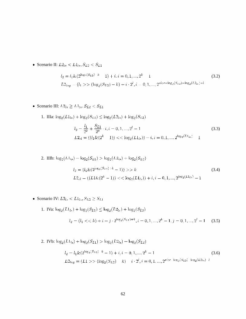
� Scenario II:L2ls < L1ls; SL2 < SL1l2 = l1&(2log2(SL2)�k � 1) + i; i = 0; 1; :::; 2k � 1 (3.2)L2tag = (l1 >> (log2(SL2)� k) + i � 2l; i = 0; 1; :::; 2size�log2(SL2)�log2(L2ls)�l� Scenario III:L2ls � L1ls; SL2 < SL11. IIIa: log2(L1ls) + log2(SL1) � log2(L2ls) + log2(SL2)l2 = l12k + SL12k � i; i = 0; 1; :::; 2l � 1 (3.3)L2cl = ((l1&(2k � 1)) << log2(L1ls)) + i; i = 0; 1; :::; 2log2(L1ls) � 12. IIIb: log2(L1ls) + log2(SL1) > log2(L2ls) + log2(SL2)l2 = (l1&(2log2(SL2)+k � 1)) >> k (3.4)L2cl = ((L1&(2k � 1)) << log2(L1ls)) + i; i = 0; 1; :::; 2log2(L1ls) � 1� Scenario IV:L2ls < L1ls; SL2 � SL11. IVa: log2(L1ls) + log2(SL1) � log2(L2ls) + log2(SL2)l2 = (l1 << k) + i+ j � 2log2(SL1)+k; i = 0; 1; :::; 2k � 1; j = 0; 1; :::; 2l � 1 (3.5)

2. IVb: log2(L1ls) + log2(SL1) > log2(L2ls) + log2(SL2)l2 = l1&(2log2(SL2)�k � 1) + i; i = 0; 1; :::; 2k � 1 (3.6)L2tag = (L1 >> (log2(SL2)� k) + i � 2l; i = 0; 1; :::; 2size�log2(SL2)�log2(L2ls)�l62

Cases I, IIIa

L1 cache line index

L2 cache line index

L1 tag

L2 tag

L1 cache set index

L2 cache set index

l k

Cases II, IVb

L1 cache line index

L2 cache line index

L1 tag

L2 tag

L1 cache set index

L2 cache set index

l k

Case IIIb

L1 tag

L2 tag

L1 cache set index

L2 cache set index

l

L1 cache line index

L2 cache line index

k

Case IVa

L1 tag

L2 tag

L1 cache line index

L2 cache line index

k

L1 cache set index

L2 cache set index

l

Figure 3.1: Different coloring scenarios considering two cache levels wherek =j log2(L2ls) � log2(L1ls) jandl =j (log2(SL2) + log2(L2ls))� (log2(SL1) + log2(L1ls)) j.

where& denotes a bit-wise AND operation,>> a right shift operation,<< a left shift operation,k =jlog2(L2ls)� log2(L1ls) j, l =j (log2(SL2)+ log2(L2ls))� (log2(SL1)+ log2(L1ls)) j andsize is the address

width in bits. Fig. 3.1 illustrates the above cases.

Given a L3 cache, the number of valid L3 cache indices is givenby the exact same formulas presented

above, provided that we replace L1 with L2, and L2 with L3. We can extend this further to provide a valid

mapping for an arbitrary number of cache levels. However, the number of valid colors increases as the level

of the cache increases. For example, the total number of valid L3 indices becomes:j (l1; l2) j �2l wherel =j (log2(SL3) + log2(L3ls))� (log2(SL2) + log2(L2ls)) j andj(l1; l2)j is the number of validl1; l2 pairs of

colors for the procedure under investigation.

If the L1 and L2 caches have the same cache line size thenk = 0 andl =j log2(SL2)� log2(SL1) j. Cases

63

I, IIIb and IVa become equivalent and provide the following valid L2 colors as follows:l2 = l1 + SL1 � i; i = 0; 1; :::; SL2SL1 � 1 (3.7)

which agrees with the findings in [103]. Cases II, IIIa and IVblead to a single L2 valid color, given by:l2 = L1&(SL2 � 1) (3.8)

Multiple cache line coloring is accomplished by traversingthe sorted popular edge list. The L1 cache

coloring process is equivalent to that presented in chapter2. L2 cache line coloring is performed after fixing

the L1 colors for a given procedure pair. L2 cache placement is performed only after L1 placement. Whenever

we place a procedure in L1 we place it in L2. Whenever we reposition a group of procedures in L1, we

reposition the same group in L2. Since we do not form compoundnodes in the L2 address space as we do in

L1, we reposition one procedure from the group at a time. Thisdemand-driven approach for L2 coloring is

primarily enforced in order to keep the algorithmic complexity low. Furthermore, popular procedures should

be mapped in L2 with no conflicts to ensure that any remaining L1 conflicts between them will be serviced by

the L2 cache instead of the main memory or the L3 cache. The pseudo-code of the algorithm is shown in Fig.

3.2.

During the edge traversal we encounter four cases:� Case I: ProceduresP1 andP2 are not colored. We place in them in the L1 cache using the firstavailable

L1 colors. The larger procedure is placed first. A new compound node is formed consisting of these two

procedures. L2 cache mapping is also performed using the numerically lowest valid L2 valid color.� Case II: Both proceduresP1 andP2 are mapped but belong to different compound nodes. After placing

the smaller node according to the heuristics described in section 2.4, we consider L2 cache placement.

Suppose thatP1 belongs to the smaller compound node. We first select an L2 valid color forP1 so that

L2 cache conflicts, and the total distance between procedures in the larger compound node andP1, are

minimized. We then remap the remaining procedures in the smaller compound node so that L2 color

conflicts, and the distance between this node andP1, become minimal. Finally, the two compound nodes

are merged into a single node.� Case III: One procedure is mapped and the other is not. We firstplace the unmapped procedure, (e.g.,P1) in the L1 cache, as in the original algorithm. We then iterate over all valid L2 cache colors forP1,and select the one generating minimum number of L2 cache conflicts and having the shortest distance

betweenP1 andP2.64

Input: list of popular edges ledge,Sort ledge on decreasing weight orderforeach e in ledgesrc = source(e), dst = destination(e);

if (src 6= mapped and dst 6= mapped) /* Case I */Assign L1 cache colors to src and dst;Both procedures are assigned to their valid L2 colors closest to the start of L2 cache address space;

elseif ((src == mapped) and (dst == mapped) and (Csrc 6= Cdst)) /* Case II */select p = dst or src based on minimum size of their compound node;Re-assign L1 cache colors to src and dst; setproc = NULL;best c = find color list(p,list of nodes in large compound node); assign p to best c color in L2;Insert p to list setproc;foreach procedure s 6= p in small compound nodebest c = find color list(s,setproc); assign s to best c color in L2;

Insert s to list setproc;endfor

elseif (only one of the src; dst is mapped (e.g. dst)) /* Case III */Assign L1 cache colors to src;best c = find color pair(src; dst); assign src to best c color;

elseif ((src == mapped) and (dst == mapped) and (Csrc == Cdst)) /* Case IV */if (color conflicts(src; dst) exist)

Select one procedure p from src; dst and re-assign L1 cache colors;if (p has been recolored in L1)best c = find color list(p,Csrc); assign p to best c color;endif

endifendif

endfor

Figure 3.2: Multiple-level cache line coloring algorithm.� Case IV: Both proceduresP1 andP2 are mapped and belong to the same compound node. If L1 cache

color conflicts occur, the algorithm attempts to reorganizethe nodes in the L1 address space, as described

in section 2.4. If the selected procedure has been remapped in L1, we adjust the L2 cache coloring for

bothP1 andP2 by finding the pair of valid L2 colors that minimize both the number of L2 cache conflicts,

and the distance between procedures in the compound node.

No backtracking from the L1 cache coloring decisions is performed when searching for an L2 color assign-

ment. This is done in order to give priority to the L1 mapping.Notice also that the selection of the L2 mapping

is subject to both coloring and page locality constraints. Every time we search through valid L2 colors, we are

looking for the color that minimizes (or eliminates) both conflicts and distance in the L2 cache address space

between the procedures under consideration.

65

function find color pair(node a, node b)min distance = 1; min overlap = 1;foreach (valid l2 color(a))overlap = find L2 overlap(a; b); distance = abs(l2 color(a) - l2 color(b));

if (overlap � min overlap and distance � min distance)best color = l2 color(a); min distance = distance; min overlap = overlap;endif

endforreturn(best color);endfunction

function find color list(node a, list s)min distance = 1; min overlap = 1;foreach (valid l2 color(a))overlap = find L2 overlap(s); distance =

P8b2s abs(l2 color(a) - l2 color(b));if (overlap � min overlap and distance � min distance)best color = l2 color(a); min distance = distance; min overlap = overlap;endif

endforreturn(best color);endfunction

Figure 3.3: Multiple-level cache line coloring algorithm (continued).


The complexity of the two-level cache coloring algorithm attains the same complexity as the algorithm for

single level cache coloring, except for the terms associated with coloring on the 2nd level cache. As discussed

in section 2.4.1, the computational order of the single level cache coloring ispe � (np+np �L1+L1 � log(L1)),wherepe is the number of popular edges,np is the number of neighboring procedures andL1 is the number

of L1 cache sets (or colors). Case I takes a constant number ofsteps. Case III needs to iterate over all L1

colors to computeovd in L1 cache and check for conflicts between the two procedures. In order to perform L2

coloring, we have to check every valid L2 color for color conflicts (between the two procedures) and select the

color according to the heuristic described in section 3.2. The complexity of this step depends on (3.7). For a

cache hierarchy that falls under scenario I, the complexityof this step becomes2l �L2, with l =j (log2(SL2) +log2(L2ls)) � (log2(SL1) + log2(L1ls)) j, andL2 being equal to the number of L2 colors. Since this term

solely depends on the L1 and L2 cache organizations, it is considered independent of the problem size.

In case II we iterate over the L1 colors to check for conflicts,iterate over the members of the selected

compound node to adjust the L1 colors once a new node positionhas been found, and perform a similar loop

to merge the two compound nodes. When L2 coloring has to be performed some additional factors must be

added. First, we must iterate over all valid L2 colors (see scenario I in (3.7)), where in each iteration we check

66

for conflicts between the procedure of the smaller node (thatis being remapped) and all members of the larger

node. In addition, each iteration includes a loop over all large node members to compute the distance between

them and the procedure under investigation. The total complexity is2l � (cnp+ (L2 + cnp � L2)). Given thatlandL2 are independent of the problem size, the complexity becomes2l � cnp(L2 + 1) + 2l � L2 = O(cnp).

An additional step is involved with adjusting the L2 colors of the remaining procedures in the small node so

that conflicts between them are minimized. Notice that the small node may be repositioned in L1, so adjusting

the position of its members in L2 is essential. This step requires a pass over all the members of the node. In

each step, an amount of work equivalent to2l � (cnp + (L2 + cnp � L2)) is required (for all valid L2 colors

check for conflicts and compute the distance). The complexity is cnp � (2l � cnp(L2 +1)+ 2l �L2) = O(cnp2).Overall, Case II is in the order ofO(cnp2).

Case IV requires a number of steps equal tonp+cnp+np�L1+L1 �log(L1) for L1 cache coloring. In order

to perform L2 coloring in Case IV we iterate over all valid L2 colors, check for conflicts between the selected

procedure and the remaining members of the compound node andcompute the distance between them. The

total cost is2l �(cnp+cnp�L2). Overall, Case IV is in the order ofO(cnp). Given the complexities of each case

and the main loop (which ispe), the complexity of the multiple cache coloring algorithm becomesO(cnp2 �pe).The upper bound isO(p4), assuming thatcnp � p andpe � p2. The first assumption is asymptotically true

because after a point, a single compound node will hold all popular procedures. However, for a large number of

iterations,cnp will be smaller thanp. As we mentioned above,pe, is significantly smaller thanp2 first because

of the nature of the graph (even a CMG is not fully connected),and second because of our pruning step which

eliminates 90% of the generated edges on the average.

3.3 Main Memory-based Procedure Placement Algorithm

The next step after placing procedures in the cache hierarchy is to determine their main memory position

by assigning memory offsets. The memory placement algorithm must now consider all colors assigned to a

procedure before selecting a memory address. The pseudo-code for the popular procedure placement algorithm

is shown in Fig. 3.4.

Our algorithm places popular procedures in a memory hierarchy containing two cache levels and uses the

same main loop as the one shown in Fig. 2.8. Popular procedures are allocated to array slots based on their

assigned L1 and L2 cache colors. We use two arrays, each equalin size to the address space of a cache. Two

indices,l1 color andl2 color, are initialized to 0. We traverse the two arrays in an attempt to find a procedure

to map. Given a pair of values for the indices, we find the set ofprocedures that are assigned to the cache colors

corresponding to the index values. If the set is empty we advance by 1 the index that corresponds to the cache

67

Input: list of popular procedures lprop,array of lists of procedures ca1[L1 CACHE SETS],array of lists of procedures ca2[L2 CACHE SETS]foreach proc in lprop

Insert proc in ca1[l1 cache color(proc)]; /* l1 cache color returns the color of proc in L1 cache */Insert proc in ca2[l2 cache color(proc)]; /* l2 cache color returns the color of proc in L2 cache */

endforl1 color = l2 color = 0, mm index = 0, mapped procs = 0;while (mapped procs 6= size(lprop))find candidate = FALSE;

while (find candidate == FALSE)proc = select proc(l1 color; l2 color; prev proc);if (proc == NULL)

if (L1 CACHE LINE SIZE > L2 CACHE LINE SIZE)l2 color = (l2 color + 1) mod L2 CACHE SETS;get next valid l1 color;

else if (L1 CACHE LINE SIZE � L2 CACHE LINE SIZE)l1 color = (l1 color + 1) mod L1 CACHE SETS;get next valid l2 color;

endifelsefind candidate = TRUE;endif

endwhilecompute gap between proc and prev proc;memory offset(proc) = mm index+ gap;mm index = mm index+ gap+ size(proc);delete proc from ca1[l1 color]; ca2[l2 color] lists; mapped procs++;l1 color = extract color(mm index); l2 color = extract color(mm index);prev proc = proc;

endwhile

Figure 3.4: Popular procedure memory placement algorithm after performing two-level cache coloring (con-tinued).

with the minimum cache line size, find the next valid value forthe other index and try again. Notice that we

can not advance the other index by 1 since the two partially define each other, as is shown in Fig. 3.1. If we

advancel1 color, we have to advancel2 color to point to the next valid value according to the formulas listed

in section 3.2. If we advancel2 color we have to find its unique equivalentl1 color in the L1 cache.

If the set of procedures mapped to a specific (l1 color; l2 color) pair contains multiple candidates, we select

the one that is connected by the smallest CMG edge weight to the previously mapped procedure. If there are

no CMG edges between the candidates and the previously mapped procedure, we select one procedure from

the available pool of candidates by random. When an candidate has been found, we compute the memory gap

between the candidate and the procedure previously mapped.The gap size is computed as follows: assume

68

function select proc(int l1 color; l2 color, node prev proc)set s = ca1(l1 color) \ ca2(l2 color);if (s == ;)

return(NULL);else

find proc 2 s so that CMG edge weight(proc; prev proc) = minimum;endifif (proc == NULL)

randomly select proc from s;endifif (gap(proc; prev proc) > PAGE SIZE)

foreach (valid l2 color(proc))if (gap(proc; prev proc) � PAGE SIZE)l2 color = l2 color(proc); break;endif

endforendifreturn(proc);

end function

Figure 3.5: Popular procedure memory placement algorithm after performing two-level cache coloring.

that l1 and l2 are the colors of the candidate procedure. Letmm index be the memory address associated

with the end of the previously mapped procedure, andk the difference in bits between the line sizes of L1

and L2 caches,k =j log2(L2ls)� log2(L1ls) j. The gap size is computed by specifying the memory address,new mm index, for the candidate procedure.new mm index has to be as close as possible tomm index to

minimize the gap size. The address must also be valid since ithas to satisfy both the L1 and L2 cache coloring.

The high order (tag field) bits ofnew mm index are specified bymm index:max size = max(log2(L1ls) + log2(Sl1); log2(L2ls) + log2(Sl2)) (3.9)hobits = (mm index� max size)� max sizeThe low-order bits are specified by thel1 and l2 colors. The line index bits are set to 0 to maintain cache

alignment for the procedure. The new memory address is then computed by combining the high and low order

bits. The gap is the difference betweennew mm index andmm index.min size = min(log2(L1ls) + log2(Sl1); log2(L2ls) + log2(Sl2)) (3.10)lowbits = 8<: ((l2� k) j l1)� min size if log2(L2ls) � log2(L1ls)((l1� k) j l2)� min size if log2(L1ls) > log2(L2ls)69

new mm index = 8<: lowbits+ highbits if (lowbits+ highbits) � mm indexlowbits+ highbits+ (1� max size) if (lowbits+ highbits) > mm indexgap = new mm index�mm indexIf the gap size is larger than the page size, then we iterate over all available L2 cache colors for that

procedure and select the one that creates a gap that is smaller than a page. If this is not possible, we keep the

original L2 mapping. This step is taken since popular procedures approximate the most frequently executed

part of the application and we prefer to place procedures as close to each other as possible to avoid causing

extra TLB misses or page faults. This is accomplished at the expense of selecting an inferior L2 mapping for

certain procedures.

After assigning memory offsets to all popular procedures, the algorithm fills the memory gaps with unpop-

ular and unactivated procedures. Any remaining unpopular and unactivated procedures are appended to the end

of the modified executable. Table 3.1 shows the total gap sizein Kb after mapping popular (columns 2-5) and

all procedures (columns 6-8). The numbers in columns 6-8 represent the total amount of extra empty space

inserted in the reordered executable. The two numbers per column correspond to the reordering configuration

without and with basic block reordering.

Program Gap after pop (in Kb) Final gap size (in Kb)CG TRG CMG CG TRG CMG

perl 5.3/25.6 23.6/22.1 25.8/24.3 0.2/0.2 0.3/0.2 0.2/0.3gcc 837/600 2221/2160 1553/1417 1.8/2.1 1550/1489 773/636edg 302/186 1020/748 326/258 1.4/1.4 3.9/4.7 1.9/2.0gs 485/382 1137/903 1200/1012 2.3/2.4 3.9/4.5 4.0/4.4troff 146/79.9 406/535 360/369 0.5/0.6 44.2/173 1.4/5.0eqn 70.4/56.6 295/263 179/122 0.2/0.2 122/90 0.9/1.0ixx 132/84.2 296/234 335/256 0.3/0.4 0.9/0.9 0.8/0.9eon 87.5/113 161/177 172/135 0.5/0.5 0.8/0.8 0.9/0.8porky 471/488 740/823 768/785 2.8/2.5 4.7/5.0 4.4/4.2bore 481/401 852/590 903/742 2.8/3.1 4.3/5.2 4.7/5.2lcom 51.8/66.9 54.1/60.3 71.2/68.6 0.2/0.2 0.2/0.2 0.2/0.2

Table 3.1: Size of memory gaps after two-level cache coloring and memory placement using the CG, TRGor the CMG. The total gap size is shown before (columns 2-5) and after (columns 6-8) mapping unactivatedand unpopular procedures. Each column displays the gap sizewhen basic block reordering does not apply andwhen it precedes cache coloring.

70

If we compare the numbers with those extracted from single cache coloring in Table 2.4, we can verify

that placing procedures in 2 levels of cache spreads procedures in the memory address space even more so.

Although the final size of the executable is not severely increased (except for the TRG/CMG-based layouts on

gcc), the number of gaps among the popular procedure set is quite significant. The numbers are larger for the

temporal-based orderings since they have to color and placea larger number of popular procedures. Perl and

lcom does not cause a significant increase because the size ofthe popular procedure set (with or without basic

block reordering) is small and fits in the L1 cache. The amountof space depends, not only on the heuristics we

used, but also on the L1 cache size and the ratio between L1 andL2 cache sizes, as it can be seen from (3.7).


The number of steps needed to allocate procedures to their array elements is stillpp, wherepp is the number

of popular procedures. The skeleton of the algorithm that places procedures in memory under L1 and L2

constraints is essentially the same as the algorithm described in section 2.5. The major difference between

the two algorithms lies in the search step, where a candidateprocedure must be found to be placed next.

Instead of looking at one array, we must now simultaneously query two arrays to satisfy both L1 and L2 cache

assignments. This adds a constant factor to the complexity of the algorithm since both indices are updated in

each iteration of the searching algorithm. Instead of traversing all L1 colors, we now visit a number of colors

equal tomax(L1; L2) whereL1 andL2 are the total number of L1 and L2 colors, respectively. Recoloring in

L2 in order to avoid large gaps in the executable requires iterating over all L2 valid colors. According to the

upper bound of the algorithm described in subsection 2.4.1 and scenario I in (3.7) wheremax(L1; L2) = L2,the cost of the algorithm becomesL2 � 2l � pp2, which is still on the order ofO(pp2).3.4 Experimental Results

To assess the performance improvement of multiple level cache coloring we used our modified version of

SimpleScalar v3.0 Alpha AXP tool-set to get cycle-based results for the optimized application images. We

also used the ATOM-based model for those applications whichlack of adequate support in SimpleScalar. We

compare results for all three graph models (CG, TRG and CMG),considering the following combinations:� CMG-based procedure reordering for multiple cache levels (Pmccmg)� CMG-based procedure and intra-procedural basic block reordering for multiple cache levels (Pbbmccmg)� TRG-based procedure reordering for multiple cache levels (Pmctrg )

71

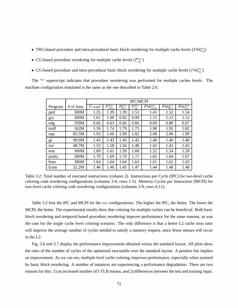
� TRG-based procedure and intra-procedural basic block reordering for multiple cache levels (Pbbmctrg)� CG-based procedure reordering for multiple cache levels (Pmccg )� CG-based procedure and intra-procedural basic block reordering for multiple cache levels (Pbbmccg )

The mc superscript indicates that procedure reordering was performed for multiple caches levels. The

machine configuration simulated is the same as the one described in Table 2.6.

IPC/MCPIProgram # of Instr. Unopt Pmccmg Pmctrg Pmccg Pbbmccmg Pbbmctrg Pbbmccgperl 300M 1.25 1.39 1.39 1.53 1.41 1.52 1.54gcc 300M 1.01 1.00 0.92 0.99 1.15 1.13 1.12edg 350M 0.66 0.63 0.66 0.66 0.69 0.80 0.67troff 162M 1.59 1.74 1.79 1.75 1.90 1.93 1.82eqn 82.5M 1.93 1.60 1.99 1.82 2.08 2.06 1.99

gs 99.6M 1.43 1.43 1.43 1.42 1.40 1.40 1.40ixx 48.7M 1.53 1.58 1.56 1.48 1.43 1.43 1.43eon 300M 1.69 1.61 1.59 1.68 1.52 1.54 1.59porky 300M 1.70 1.69 1.70 1.71 1.65 1.64 1.67bore 300M 1.64 1.64 1.64 1.63 1.61 1.62 1.63lcom 32.2M 1.46 1.46 1.45 1.47 1.44 1.48 1.48

Table 3.2: Total number of executed instructions (column 2). Instructions per Cycle (IPC) for two-level cachecoloring code reordering configurations (columns 3-9, rows1-5). Memory Cycles per Instruction (MCPI) fortwo-level cache coloring code reordering configurations (columns 3-9, rows 6-11).

Table 3.2 lists the IPC and MCPI for themc configurations. The higher the IPC, the better. The lower the

MCPI, the better. The experimental results show that coloring for multiple caches can be beneficial. Both basic

block reordering and temporal-based procedure reorderingimprove performance for the same reasons, as was

the case for the single cache level coloring scenario. The only difference is that a better L2 cache miss ratio

will improve the average number of cycles needed to satisfy amemory request, since fewer misses will occur

in the L2.

Fig. 3.6 and 3.7 display the performance improvement obtained versus the standard layout. All plots show

the ratio of the number of cycles of the optimized executableover the standard layout. A positive bar implies

an improvement. As we can see, multiple level cache coloringimproves performance, especially when assisted

by basic block reordering. A number of instances are experiencing a performance degradation. There are two

reasons for this: 1) an increased number of I-TLB misses, and2) differences between the test and training input.

72

0 5 10 15 20 25

mc−cmg

mc−trg

mc−cg

mc−bb−cmg

mc−bb−trg

mc−bb−cg

Cycle reduction for perl

Performance improvement (%)−15 −10 −5 0 5 10 15

mc−cmg

mc−trg

mc−cg

mc−bb−cmg

mc−bb−trg

mc−bb−cg

Cycle reduction for gcc


0 2 4 6 8 10 12 14 16 18

mc−cmg

mc−trg

mc−cg

mc−bb−cmg

mc−bb−trg

mc−bb−cg

Cycle reduction for troff

Performance improvement (%)−25 −20 −15 −10 −5 0 5 10

mc−cmg

mc−trg

mc−cg

mc−bb−cmg

mc−bb−trg

mc−bb−cg

Cycle reduction for eqn


−5 0 5 10 15 20

mc−cmg

mc−trg

mc−cg

mc−bb−cmg

mc−bb−trg

mc−bb−cg

Cycle reduction for edg


Figure 3.6: Cycle count reduction/increase after applyingtwo-level cache code reordering to the default codelayout. All results are generated via execution-driven simulation.

73

−1 −0.5 0 0.5 1 1.5 2 2.5 3

mc−cmg

mc−trg

mc−cg

mc−bb−cmg

mc−bb−trg

mc−bb−cg

Memory cycle reduction for gs

Performance improvement (%)−4 −2 0 2 4 6 8

mc−cmg

mc−trg

mc−cg

mc−bb−cmg

mc−bb−trg

mc−bb−cg

Memory cycle reduction for ixx


0 2 4 6 8 10 12

mc−cmg

mc−trg

mc−cg

mc−bb−cmg

mc−bb−trg

mc−bb−cg

Memory cycle reduction for eon

Performance improvement (%)−0.5 0 0.5 1 1.5 2 2.5 3 3.5 4

mc−cmg

mc−trg

mc−cg

mc−bb−cmg

mc−bb−trg

mc−bb−cg

Memory cycle reduction for porky


−0.5 0 0.5 1 1.5 2 2.5

mc−cmg

mc−trg

mc−cg

mc−bb−cmg

mc−bb−trg

mc−bb−cg

Memory cycle reduction for bore

Performance improvement (%)−2 −1.5 −1 −0.5 0 0.5 1 1.5

mc−cmg

mc−trg

mc−cg

mc−bb−cmg

mc−bb−trg

mc−bb−cg

Memory cycle reduction for lcom


Figure 3.7: Memory cycle count reduction/increase after applying two-level cache code reordering to the defaultcode layout. All results are generated via trace-driven simulation.

74

Performance for gs is improved since reordering in the L2 cache paid off, even for the CG-based scenario. The

only benchmark for which execution time increases when basic block reordering is enabled is lcom (mc�bb�cgconfiguration). This is because the limiting factor in lcom is its small working set captured by the CG (4.5Kb),

compared to that found by either the TRG (15.8Kb) or the CMG (15.2Kb). Multiple level cache coloring does

not redefine the working set of the application.

−25 −20 −15 −10 −5 0 5 10 15 20

gcc

perl

troff

eqn

edg

Cycle reduction


mc−bb−cmgmc−cmgsc−bb−cmgsc−cmg

−8 −6 −4 −2 0 2 4 6 8 10 12

gs

porky

bore

eon

ixx

lcom

Memory cycles reduction


mc−bb−cmgmc−cmgsc−bb−cmgsc−cmg

Figure 3.8: Comparison of the cycle count reduction after applying single and two-level cache code reorderingto the default code layout. The set of results shown on the left (right) is generated via execution-driven (trace-driven) simulation.

Fig. 3.8 compares the performance improvement of single cache coloring against the multiple cache col-

oring algorithm in terms of number of saved clock cycles. CMG-based results are shown only. Multiple level

cache coloring does not always improve upon single level, and the best configuration depends on the applica-

tion. We identified three reasons for this. First, a large number of popular procedures are recolored in the L2

cache during memory placement in order to minimize memory gaps. Although the new L2 colors preserve the

L1 coloring, they may result in a higher number of L2 cache misses at the expense of better page locality. The

amount of L2 re-coloring depends on an application’s popular procedure set size, average popular procedure

size and graph edge weights. Table 3.3 shows the total numberof popular procedures (columns 2-5), and the

number of popular procedures (columns 6-14), whose L2 colorhas been reevaluated in an attempt to reduce

code size bloat. The significant number of procedures recolored in L2 (shown in Table 3.3), indicates that most

of the L2 coloring work has been undone.

The second reason is related to the first. The number of I-TLB misses and allocated pages varies across

the code reordering configurations we examined. The greaterthe code size increase, the higher the probability

that the number of I-TLB misses will rise. As mentioned above, rearranging code in the L2 cache lowers

75

Pop procs Pop procs with L2 color reevaluationProgram CG TRG CMG Pmccg Pmctrg Pmccmg Pbbmccg Pbbmctrg Pbbmccmgperl 20 21 23 7 8 21 13 13 13gcc 254 657 481 226 594 437 229 602 428edg 106 358 138 91 324 121 102 327 122gs 199 380 415 183 347 382 179 352 376troff 71 201 182 64 180 162 68 185 170eqn 41 145 99 40 126 96 40 120 95ixx 36 82 87 31 70 80 34 71 80eon 55 89 90 49 80 72 50 80 76porky 175 296 290 143 259 262 160 265 269bore 171 299 308 162 282 281 163 266 278lcom 30 43 40 25 37 39 27 40 39

Table 3.3: Revealing the amount of L2 color reevaluation: total number of popular procedures for CG, TRGand CMG (columns 2-4), number of popular procedures subjectto L2 color reevaluation for CG, TRG andCMG, when no bb-reordering has been performed (columns 5-7)and when bb-reordering precedes two-levelcache coloring (columns 8-10).

page locality, and the trade-off between the two has to be carefully considered. Overall, the positive impact

of multiple level cache coloring on performance (even when compared to single cache coloring) underlines its

viability in a code reordering framework, even for applications that do not significantly stress the L2 cache with

their instruction working set.

The third reason is that both data and instructions are sharing the L2 cache resource. Interference between

the two is not taken into account in this work. Applications with large data sets that do not fit in the L2 cache

will cause a large number of misses, possibly replacing instructions. Therefore, someone has to rearrange both

code and data in the L2 cache address space in order to improveits utilization. Furthermore, we believe that if

we consider jointly data and instructions we may be able to relieve some of the pressure applied from the page

sensitive heuristics on the L2 coloring process. Although data reordering is outside the scope of this thesis it

should be considered as future work.

Fig. 3.9 and 3.10 display the L1/L2 cache miss ratios for all simulated configurations. The L2 cache

miss ratio is computed over all references serviced by the L2only and does not include L1 cache hits in the

denominator. Again, the impact of the coloring algorithm isobvious on both L1 and L2 caches. Notice that we

should not expect to see a lower L2 cache miss ratio when transitioning from thesc to themc specification due

to the way the L2 cache miss ratio is computed. Even if we recompute the L2 cache miss ratio, data and code

interference will prevent us from detecting any noticeablevariations due to better code placement in the L2.

76

0 2 4 6 8 10 12 14

unopt

mc−cmg

mc−trg

mc−cg

mc−bb−cmg

mc−bb−trg

mc−bb−cg

L1/L2 cache miss ratios for perl

L1 = 311.9ML2 = 8.6M

L1 = 309.7ML2 = 5.8M

L1 = 309.4ML2 = 5.5M

L1 = 307.5M L2 = 3.1M

L1 = 310.8ML2 = 4.8M

L1 = 309.5M L2 = 3,4M

L1 = 308.9M L2 = 3.0M

percent (%)

L1L2

0 1 2 3 4 5 6 7 8

unopt

mc−cmg

mc−trg

mc−cg

mc−bb−cmg

mc−bb−trg

mc−bb−cg

L1/L2 cache miss ratios for gcc

L1 = 315.5M L2 = 8.9M

L1 = 316.1ML2 = 9.2M

L1 = 316.4M L2 = 9.4M

L1 = 316.3ML2 = 9.2M

L1 = 314.5M L2 = 6.1M

L1 = 314.9ML2 = 6.8M

L1 = 314.8M L2 = 6.7M

percent (%)

L1L2

0 0.5 1 1.5 2 2.5 3 3.5 4

unopt

mc−cmg

mc−trg

mc−cg

mc−bb−cmg

mc−bb−trg

mc−bb−cg

L1/L2 cache miss ratios for troff

L1 = 163.8ML2 = 3.7M

L1 = 163.6M L2 = 2.1M

L1 = 164.3ML2 = 2.0M

L1 = 164.0ML2 = 2.4M

L1 = 166.2M L2 = 1.4M

L1 = 166.1M L2 = 1.3M

L1 = 164.4M L2 = 1.9M

percent (%)

L1L2

0 0.5 1 1.5 2 2.5

unopt

mc−cmg

mc−trg

mc−cg

mc−bb−cmg

mc−bb−trg

mc−bb−cg

L1/L2 cache miss ratios for eqn

L1 = 83.4ML2 = 755K

L1 = 83.2ML2 = 1.8M

L1 = 83.6ML2 = 555K

L1 = 83.1ML2 = 1.0M

L1 = 85.2ML2 = 344K

L1 = 85.3ML2 = 398K

L1 = 84.4ML2 = 592K

percent (%)

L1L2

0 2 4 6 8 10 12 14

unopt

mc−cmg

mc−trg

mc−cg

mc−bb−cmg

mc−bb−trg

mc−bb−cg

L1/L2 cache miss ratios for edg

L1 = 370.7M

L2 = 19.1ML1 = 371.1M L2 = 18.0M

L1 = 370.6ML2 = 17.7M

L1 = 371.0ML2 = 17.9M

L1 = 370.3M L2 = 16.4M

L1 = 368.4ML2 = 14.0M

L1 = 371.1M L2 = 17.1M

percent (%)

L1L2

Figure 3.9: L1/L2 cache miss ratios of both the optimized andthe unoptimized executables. The number ofreferences to L1/L2 is appended on top of every bar. All results are generated via execution-driven simulation.

77

0 0.5 1 1.5 2 2.5 3 3.5 4

unopt

mc−cmg

mc−trg

mc−cg

mc−bb−cmg

mc−bb−trg

mc−bb−cg

L1/L2 cache miss ratios for gs

L2 = 1.0M

L2 = 1.0M

L2 = 1.0M

L2 = 949K

L2 = 785K

L2 = 750K

L2 = 703K

percent (%)

L1L2

0 2 4 6 8 10 12 14

unopt

mc−cmg

mc−trg

mc−cg

mc−bb−cmg

mc−bb−trg

mc−bb−cg

L1/L2 cache miss ratios for ixx

L2 = 810K

L2 = 1.13M

L2 = 966K

L2 = 503K

L2 = 154K

L2 = 162K

L2 = 198K

percent (%)

L1L2

0 0.5 1 1.5 2 2.5 3

unopt

mc−cmg

mc−trg

mc−cg

mc−bb−cmg

mc−bb−trg

mc−bb−cg

L1/L2 cache miss ratios for eon

L2 = 9.2M

L2 = 6.3M

L2 = 5.5M

L2 = 8.8M

L2 = 2.7M

L2 = 3.7M

L2 = 5.7M

percent (%)

L1L2

0 0.5 1 1.5 2 2.5 3 3.5

unopt

mc−cmg

mc−trg

mc−cg

mc−bb−cmg

mc−bb−trg

mc−bb−cg

L1/L2 cache miss ratios for porky

L2 = 8.6M

L2 = 7.9M

L2 = 8.5M

L2 = 8.0M

L2 = 6.1M

L2 = 6.1M

L2 = 7.3M

percent (%)

L1L2

0 0.5 1 1.5 2 2.5 3 3.5

unopt

mc−cmg

mc−trg

mc−cg

mc−bb−cmg

mc−bb−trg

mc−bb−cg

L1/L2 cache miss ratios for bore

L2 = 7.5M

L2 = 6.6M

L2 = 7.2M

L2 = 6.7M

L2 = 5.5M

L2 = 5.9M

L2 = 6.1M

percent (%)

L1L2

0 0.5 1 1.5 2 2.5 3 3.5 4 4.5 5

unopt

mc−cmg

mc−trg

mc−cg

mc−bb−cmg

mc−bb−trg

mc−bb−cg

L1/L2 cache miss ratios for lcom

L2 = 373K

L2 = 404K

L2 = 359K

L2 = 407K

L2 = 330K

L2 = 476K

L2 = 493K

percent (%)

L1L2

Figure 3.10: L1/L2 cache miss ratios of both the optimized and the unoptimized executables. The number ofreferences to L2 is also appended on top of every bar. All results are generated via trace-driven simulation.

78

However, multiple cache coloring affects the L1 cache miss ratio. Notice that our simulated model does not

supply any form of explicit instruction prefetching between the L1 I-cache and the unified L2 cache. Therefore,

no improvement occurs because L2 hits, that would otherwisemiss in L2, prefetch useful data into L1.

However, speculative execution supported by branch prediction, is modeled. Speculative execution is

known to have a rather positive effect on I-cache miss ratio via implicit prefetching of wrong path instructions

[104]. The extra amount of speculation detected, after transitioning to multiple cache level coloring (gcc exe-

cutes 300K more speculative instructions in themc� bb� cmg configuration compared to thesc� bb� cmgconfiguration) is responsible for the slight improvements in the L1 I-cache miss ratio. Code reordering also

negates the negative effects of reads, from the wrong speculative path, producing cache pollution. The small

increases in the number of speculative I-cache accesses is due to the conservative nature of the I-fetch unit

which stops fetching at the boundaries of a cache line or whena conditional branch is predicted taken.

I-TLB misses/Allocated pagesProgram Unopt Pmccmg Pmctrg Pmccg Pbbmccmg Pbbmctrg Pbbmccgperl 24/2423 16/2402 16/2382 16/2362 15/2321 15/2309 17/2303gcc 1797/870 37745/980 70434/1078 7611/886 27396/964 51144/1059 1647/879edg 10532/651 7723/661 144990/668 11182/667 6859/665 36290/665 13476/667troff 53/181 57/185 63/191 38/166 58/186 79/207 35/163eqn 29/58 32/58 47/73 23/52 27/56 43/69 22/51

gs 91/302 1608/349 1196/359 95/287 403/340 2140/334 83/277ixx 36/181 51/194 46/189 24/167 41/184 38/181 18/161eon 40/73 26/50 24/48 13/37 21/45 26/50 17/41porky 78/239 113/274 110/271 68/229 113/274 120/281 70/231bore 75/277 961/333 159/328 78/277 119/315 97/298 68/270lcom 43/202 25/175 25/175 25/175 25/175 25/175 25/175

Table 3.4: I-TLB misses and number of allocated pages for both the unoptimized case and the executablesoptimized with different configurations of two-level cachecode reordering.

Table 3.4 shows the number of I-TLB misses and the number of allocated pages for each application. Due to

the aggressive reordering produced by the multiple cache coloring algorithm, the number of I-TLB misses and

number of allocated pages increased in several experiments. The sharp rise of I-TLB misses in certain cases,

such as edg and gcc, clearly motivates the need for further tuning of the page-sensitive heuristics. Previous

work on page coloring has successfully utilized temporal information in [65], and thus could be employed to

assist popular procedure memory placement. Page locality tends to be worse before basic block reordering,

although that depends on the memory gaps left after placing popular procedures in both caches (see Table 3.1).

79

3.5 Summary

We have modified the cache conscious procedure placement algorithm presented in chapter 2 to consider col-

oring procedures on multiple cache levels. The sufficient and necessary conditions for preserving theith-level

cache mapping when mapping to thei + 1th-level cache are also described. These conditions guarantee that

mapping between two successive cache levels is retained regardless of the caches organizations. We have

also presented a modified memory placement algorithm that both takes into account coloring constraints from

multiple cache levels and attempts to prevent deterioration of page locality.

Experimental results showed that optimized code layouts based on multiple cache level mapping, raised

performance to levels similar to those achieved by single cache level configurations. Only in some cases, per-

formance improvement over the single cache coloring approach is noticeable. Prefetching between successive

cache levels, page coloring, larger working sets and instruction/data combined placement are some of the issues

that can further exploit the benefits from an improved mapping across multiple cache levels.

80

Chapter 4

Indirect Branch Classification and

Characterization

Applications developed under the OOP execute a large numberof indirect branches. These branches support

polymorphic procedure calls in OOP and depending on the implementation language, their frequency can be

substantial. At the same time, indirect branches impose a natural impediment in microprocessors that explore

ILP via control speculation because they always disrupt sequentiality. In this chapter we study the behavior of

indirect branches found in C and C++ applications. We characterize branches using both static analysis and

profile information. The static analysis is based on instruction opcode and code source usage.

Using profile information, we classify branches based on their target locality, target entropy, type and length

of path correlation, and load predictability. The goal of both partitioning schemes is to categorize branches in

a way so that each group has well-defined behavior and run-time predictability characteristics. We can then

use this information to design compiler-assisted, hardware-based hybrid indirect branch predictors consisting

of multiple components, where each component is best suitedfor one (or more) groups of branches.

4.1 Related Work

The concept of branch classification for improving branch prediction accuracy is not new. A generic form

of branch classification has already been proposed: a Return-Address Stack (RAS) for return instructions, a

CBT for branches generated by switch statements and a conventional branch predictor (e.g. BTB with 1-bit of

history) for conditional branches. P.Y. Chang et al. classified conditional branches using profile information

in order to design better hybrid predictors [105, 106]. Theypartitioned conditional branches based on their

dynamic taken rate into mostly-one-direction (either taken or non-taken) and mixed-direction branches. They

81

examined the performance of various two-level predictor configurations (PAs, GAs and gshare) and found that

highly biased branches were best predicted using a short history register length, while the remaining required a

long history length. They proposed several hybrid designs that took into consideration profile information. One

of them used a two-level branch predictor that selects between short and long history length when accessing a

PHT entry. Their selection was based on profile-guided classification. Another design used a static approach for

highly biased branches and a gshare predictor for the remaining branches. They also described solutions based

on run-time classification of branches using a table of 2-bitselector counters, similar to the approach proposed

in [107]. Each counter decides which of the two components ofthe hybrid design will be used for making a

prediction. Finally, they discussed a hybrid design, wherehighly biased branches are predicted using profile

data, and non-biased branches are fed to a predictor that uses selector counters and two component predictors.

Driesen et al. focused on identifying the predictability and correlation length of indirect branches [31, 108,

109]. They measured the correlation length by determining the number of targets (full or partial) that have to be

recorded in a Path History Register (PHR) for the branch to bebest predicted. Simulation results showed that

most indirect branches are biased towards one end of the spectrum. They need either a large or a small number

of targets in order to achieve good prediction accuracy. Theauthors also provide data for indirect branches that

implement polymorphic calls. Their findings show they change their target infrequently in time. A mechanism

that uses the previously seen target to predict the next one is usually adequate for achieving high prediction

accuracy for those branches. However, they also detected polymorphic calls that visit many targets with a

high degree of interleaving (the targets changes frequently in time). These branches require more sophisticated

mechanisms to be accurately predicted.

There are also have been several studies on the nature of polymorphic calls [19, 20, 110]. The most profound

conclusion is that polymorphic call sites tend to visit onlya few targets during the execution of the program,

with only a few sites jumping to more than 4 targets.

An empirical static analysis study of C function pointers was presented in [111, 112]. Investigating function

pointers is of interest to us because a procedure call via a function pointer is implemented with an indirect

procedure call. Although the goal of the study in [112] was toexamine function pointer usage within the

context of alias and interprocedural analysis, we benefit from the type of available information in several ways.

The results in [112] show that most applications use mainly global function pointers that are assigned in many

places throughout the program. Similar results are presented in [111]. Due to extensive aliasing, it is not only

difficult to statically disambiguate calls made with these pointers, but also to predict them correctly at run-time.

This is because frequent assignments will hurt the temporallocality of the target associated with an indirect

branch, even if the actual number of individual targets is small. Another finding was that arrays of function

pointers are implemented as jump tables. A call made via an element of that array would make run-time

82

prediction difficult, even if the target visited by each individual array element is unique. This is because the

history for the part of the array being accessed must be recorded in hardware. Also, heap-based indirect call

sites tend to have a small number of resolved callees, whereas parameter and statically initialized global call

sites have more callees [111].

4.2 Opcode and Source Code-based Indirect Branch Classification

In this section we classify indirect branches based on theiropcode and source code usage. The Alpha AXP

ISA, which is used in our study, has the following unconditional indirect branches :jsr for indirect procedure

calls, jmp for indirect jumps andret for subroutine returns1. We will not discussret instructions any further

since they are handled properly by a RAS. After examining thesource code we concluded that most of the

jsr instructions implement polymorphic calls (virtual function calls in C++ parlance), calls through function

pointers and function calls that require the use of Global Offset Tables (GOTs). A GOT is used to implement

global variable accesses andlong function calls in applications running on the 64-bit address space of the Alpha

CPU [113]. A long function call is one whose caller and callee are laid out far apart in the image so that the

offset of a direct procedure call (bsr) has inadequate support. Jmp instructions mostly resolve switch statements

although certain jmp instructions were found to access run-time tables holding various types of addresses.

4.2.1 Conventional function calls

A GOT is a run-time data structure used to collect global addresses [113]. GOTs are generated for each sep-

arately compiled module, but the linker can merge multiple GOTs as an optimization. GOT-based accesses

are those corresponding to global and static data. GOT accesses are made via the global pointer (gp) register

together with a 16-bit displacement in the Alpha AXP ISA [114]. If multiple procedures share the same GOT,

they can use the same value ofgp to perform all GOT-based accesses. Otherwise, on every procedure call, thegp must be saved and restored. The size of the application is notthe only reason behind the use of separate

GOTs values for different routines. A dynamically linked module has its own GOT which can be placed far

away from the global GOT. Access to DLL functions may be implemented via a GOT.

Conventional function calls are implemented with indirectbranches that transfer control flow to an address

that is loaded from the GOT via thegp. The following sequence illustrates the concept:

ldq pv,o3(gp) // Load the procedure value of the caller

jsr ra,(pv) // Make the procedure call1The jsr coroutinewas not found in our traces so we will not refer to it.

83

pv is the procedure value register which holds the starting memory address for the caller.ra is the return

address register which saves the return address during the call. In order to avoid this overhead, the linker

attempts to optimize the call by merging the GOTs of the caller and the callee. GOT merging eliminates the

instructions resetting thegp value of every procedure (twolda instructions, not shown here, are used to resetgp). Also, if the callee is near enough to the caller, there is noneed for the indirect branch, and a direct call

(bsr) can be used instead [114]. There exist a few additional optimizations that can be used, but we only

describe the schemes that involve an indirect branch. The linker provided with the Compaq Unix operating

system optimizes most of those calls.

Indirect branches also implement procedure calls made through function pointers. The function pointer is

loaded with the target function address from the GOT or from some other data structure of the application. It

may be a field of struct/union in C, a global/local variable, aparameter, etc. Therefore, it can be assigned the

actual function address anywhere in the program. The code sequence is identical with that shown above. The

only difference is that thegp register is used only if the pointer is accessing the GOT to locate the function

address.

4.2.2 Virtual function calls

In order to understand the run-time mechanism behind a polymorphic call, we must first examine the underlying

object model and the inheritance properties. We will focus on C++ since some of our benchmarks are written

using this language. A classD that inherits data or behavior from a classB is called subclass ofB or a derived

class ofB (see Fig. 4.1). ClassB is called a superclass ofD or a base class. If a subclass inherits from only one

(multiple) base class, then we have a case ofsingle (multiple)inheritance. The Class Hierarchy Graph (CHG)

has a node for every class, and an edge for every inheritance relationship between two classes. Two classes

that are connected via en edge are directly related. Therefore, B is a direct superclass ofD, but S is just a

superclass ofD. The object model defines the memory layout of an object. An object of classD consists of

subobjects for every superclass (direct or not) ofD, and one subobject forD [28, 42, 40]. The subobject of a

superclassX holds, among other things, the data members inherited fromX. The subobject ofD includes all

data members defined locally inD. Additional space may be inserted between the components ofan object to

satisfy alignment requirements of individual components [115].

The uppermost part of Fig. 4.1 illustrates an example of a CHGwith single inheritance, and shows the

underlying object layout for classesB andD on the right side. Besides identifying the subobjects for each

object, it is important to discuss the order of the subobjects in the object layout. Base class subobjects are

always laid out first (with the exception of a virtual base class that will be described later). For example, the

data members ofS are always found at the beginning of an object of classB, or an object of classD. In single

84

inheritance class hierarchies, objects of subclasses inherit the layout of their superclasses’s objects. Notice

that theB object has an identical layout to part of theD object. This allows the same code to be used when

accessing inherited data members.

In the case of multiple inheritance, the order of subobjectsin the derived object can not be the same as if

the derived object inherited data/behavior from each of itssuperclasses individually. Some C++ compilers use

the leftmost class rule to decide which subobject will be laid out next to the derived subobject. In Fig. 4.1, the

leftmost class in the CHG for classD isC1 class. Thus theC1 subobject is laid out before theD subobject. In

addition, the code accessing the data members defined in theC2 class can not be reused and all offsets have to

be adjusted by a constant amount. The details of this approach is beyond the scope of this thesis.

B

D

Single Inheritance

Multiple Inheritance

C1

D

C2

Virtual Inheritance

C1

D

C2

Vv v

B part

D part

D class object

C2 part

D part

D class object

C1 part

D part

C2 part

D class object

C1 part

V part

B subobject

D subobject

C1 subobject

D subobject

C2 subobject

VBPTR

VBPTR

VBPTR

C1 subobject

V subobject

D subobject

C2 subobject

SS partS subobject

B part

B class object

B subobject

S part S subobject

Figure 4.1: Object layout for class hierarchies with single, multiple and virtual inheritance.

Now consider the CHG found at the bottom of Fig. 4.1. ClassD directly inherits from bothC1 andC2,which in turn directly inherit fromV . In order to allow proper sharing of data/behavior of classV in an object

of classD, classV must be declared as avirtual base classand the inheritance relationship betweenV and its

direct subclasses,C1 andC2, is defined asvirtual inheritance[116]. This is denoted by the letterv over the

85

CHG edges in Fig. 4.1. Virtual inheritance dictates that there should be one and only oneV class subobject

in aD class object. In general, the virtual base class subobjectsare always laid out last in the object layout.

In order to access the data members/behavior of virtual baseclass subobjects, pointers are supplied for every

subobject in an object of classD. Each such pointer is called aVirtual Base PoinTeR(VBPTR), which points to

the beginning of theV subobject. A VBPTR is considered to be part of its associatedsubobject. If there exist

more than one virtual base classes, every subobject has a pointer to a table of VBPTRs, each VBPTR pointing

to a different virtual base class subobject. An alternativeway of implementing VBPTRs is with offsets. Instead

of pointing to the beginning address of the virtual base class subobject, the VBPTR of a subobject holds an

offset from the beginning of that subobject to the beginningof the virtual base class subobject. In case of

multiple virtual base classes, the VBPTR is a pointer to a table of offsets. The offset implementation requires

an arithmetic operation to access the virtual base class subobject at the expense of extra space, while a pointer

implementation requires less space but uses a memory indirect reference via a load. If a class is both an ordinary

and a virtual base class in the same object, then the object will contain two subobjects, one virtual (that will be

laid out at the end of object) and one non-virtual (which is going to be laid out according to the leftmost class

rule).

The most common way to express polymorphism in C++ is via polymorphic functions, calledvirtual func-

tions in C++ parlance. A virtual function is a member function whose invocation via a public base class

reference or pointer is resolved at run-time [116]. The particular function implementation that will be invoked

at run-time is decided upon predetermined visibility rules. Fig. 4.2 displays the different scenarios, while the

corresponding decisions are listed below. We assume that the call to be resolved isb! foo(), foo() is a virtual

function,b is a pointer to an object of classB andrt(b) is the run-time type of pointerb.� Case I :b! foo()) B :: foo()� Case II :b! foo()) 8>>><>>>: B :: foo() if (rt(b) = B) _ ((rt(b) = C) ^ (foo() is not defined in classC))C :: foo() if (foo() is defined in classC) ^ (rt(b) = C)� Case III :b! foo()) 8>>><>>>: A :: foo() if (foo() is not defined in classC) _ (rt(b) = B)C :: foo() if (foo() is defined in classC) ^ (rt(b) = C)

If an object of classB has a local implementation of functionfoo() that is also defined as non-virtual, then

this is the only function body to be invoked viab ! foo() (case I). If the local definition becomes virtual

thenb ! foo() can invoke the local copy offoo() if b points to an object of classB at run-time. Ifb points

86

B

A

C

foo()/ v:foo()/ -

foo()

foo()/ v:foo()/ -

Case I

B

A

C

foo()/ v:foo()/ -

v:foo()

foo()/ v:foo()/ -

Case II

B

A

C

v:foo()

-

foo()/ v:foo()/ -

Case III

Figure 4.2: Visibility rules for C++ virtual function call resolution.

to an object of a subclass (case II), then the implementationof that subclass will be invoked. If there is no

such implementation, then the original local copy will be called (case II). If classB does not have a local

implementation offoo(), then the implementation of its superclass will be invoked if none ofB’s subclasses

have a local copy, or ifb points to an object of classB at run-time. Ifb points to an object of a subclass and

the subclass has a local implementation, then that functionbody will be invoked. Summarizing, ifst(b) is the

static type of pointerb thenrt(b) can best(b) or a subclass ofst(b). The actual function called is always the

one that is inherited or overridden byrt(b).If a virtual function is called from an object (in C++ syntax this is equivalent toB :: foo()), then there is

no run-time overhead since the function implementation is known at compile-time [28]. A run-time resolution

mechanism is needed only if the call is made through a pointeror a reference. The actual function body

that is invoked is decided based on therun-time typeof the pointer making the call. In other words, accurately

predicting the branch making a polymorphic call is equivalent to finding the type of the object where the pointer

points to at run-time.

For C++ and Java, the most widely used run-time mechanism supporting virtual function calls is theVirtual

Function Table(VFT) [28]. Although other mechanisms have been proposed inthe literature (see [31] for a long

list), the VFT seems to be the most time and space efficient. Itcan be used only for programming languages

where the set of virtual functions available to a class is fixed at compile-time [40]. We will discuss VFT

implementations in detail since VFTs have been adopted by commercial C++ compilers such as the Compaq

C++ used in this thesis. Conceptually, the compiler generates a VFT for every class that defines or inherits

a virtual function in the CHG. A VFT can be thought of as a tableof function addresses. If an object of a

classX is permitted to invoke virtual functions either via inheritance or locally, it must have access to the VFT

providing access to those functions. This is usually done with a pointer to a VFT, widely known as aVirtual

87

PoinTeR(VPTR). An object must have a number of VPTRs, equal in numberto the number of accessible VFTs.

In general, the number of VPTRs is equal to the number of superclasses plus one more for the derived class,

except that a derived class can share a VPTR with its leftmostbase class [40, 116]2. A derived class can not

share its VPTR with a virtual base class. In single inheritance, there is a single instance of each virtual function

to which any call can be resolved. This is true whether the function is called through a pointer to an object of

the derived class, or to one of its base classes. Hence, the single set of functions associated with the derived

class can be indexed by only one VPTR shared by all subobjectsin the derived class object [116].

Fig. 4.3 illustrates the CHGs shown in Fig. 4.1, modified withvirtual function definitions. The correspond-

ing object layouts are again shown on the right side of the figure, with the VPTRs explicitly displayed.

B

D

Single Inheritance

Multiple Inheritance

C1

D

C2

Virtual Inheritance

C1

D

C2

Vv v

B part

D part

VPTR

D class object

C2 part

D part

VPTR

D class object

C1 part

D part

C2 part

VPTR

D class object

C1 part

V part

VPTR

B subobjectD subobject

VPTR

C1 subobject

D subobject

C2 subobject

VPTR

VBPTR

VBPTRC1 subobject

V subobject

D subobject

C2 subobject

v:foo()

foo()

v:foo()

bar()

v:bar()v:baz()

foo()

bar()

v:bar()

v:foo()

v:baz()

Figure 4.3: Object layout in the presence of virtual functions, inside a class hierarchy with single, multiple andvirtual inheritance.

Assume that we again need to resolve the callb ! foo(). If E is the class defining the functionfoo()that will be actually called at run-time, given the rules in (4.2), we have to perform two basic tasks: 1) transfer2When two subobjects share a VPTR, they usually share their VBPTR as well, if a VBPTR is needed.

88

control flow to the proper function body, and 2) adjust thethis pointer to point to the subobject of theE class3. The basic steps for accomplishing the two goals are as follows [42]:� Adjust thethis pointer to the subobjectX, in the object of typert(b), whose VFT contains the address

of E :: foo(). This adjustment is called anearly cast.� Access the VFT entry using the VPTR of theX subobject.� Adjust thethis pointer to point to theE subobject within the object of typert(b), only if E andX are

different. This adjustment is called alate castand is independent of an early cast.� AccessE :: foo() function via the VFT entry.

Steps 2 and 4 are always required, while steps 1 and 3 are only necessary if the inheritance is multiple

and/or virtual. Adjustments to thethis pointer are necessary because thethis pointer is the base address based

upon which all data members, VPTRs and VBPTRs are accessed. The implementation of the casts depends

on the VFT layout. A VFT is usually characterized by two parameters: 1) its height, and 2) its width. Height

indicates the number of VFT entries, while width specifies the contents of each entry. There exist two VFT

configurations based on the VFT height. The first one isVisible, where a VFT for a class contains all virtual

functions visible in that class. According to the rules explained above, the VFT will include all virtual functions

declared in that class or inherited by that class. When a VPTRis shared by subobjects of two different classes,

the VFT will contain the union of virtual functions that are visible in these classes.

The second VFT configuration is calledIntroduced, where a VFT for a class contains all introduced virtual

functions by that class. In other words, all virtual functions that are declared by that class, but not declared by

any of its base classes, are included in the VFT. Again, when aVPTR is shared by subobjects of two different

classes, the VFT will contain the union of virtual functionsthat are visible in these classes. In both schemes,

when a virtual function is overridden, the virtual functionin the VFT is the one that is in the most derived class

of the object. The introduced scheme does not duplicate VFT entries as the class hierarchy gets larger. The

total number of VFT entries for the introduced option is equal to the total number of virtual functions in the

application. If virtual or multiple inheritance occurs, the visible configuration duplicates VFT entries.

Although the introduced scheme saves space by creating the minimum number of VFT entries, it requires

additional instructions to find the VFT entry in the introducing base class’s subobject. Those instructions

perform an early cast, as mentioned before. An early cast is always a cast to a base class’s subobject. The

visible alternative never requires an early cast.3Initially, the this pointer for an object points to the beginning address of the object.

89

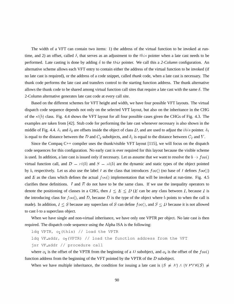
The width of a VFT can contain two items: 1) the address of the virtual function to be invoked at run-

time, and 2) an offset, called�, that serves as an adjustment to thethis pointer when a late cast needs to be

performed. Late casting is done by adding� to thethis pointer. We call this a2-Columnconfiguration. An

alternative scheme allows each VFT entry to contain either the address of the virtual function to be invoked (if

no late cast is required), or the address of a code snippet, called thunkcode, when a late cast is necessary. The

thunk code performs the late cast and transfers control to the starting function address. The thunk alternative

allows the thunk code to be shared among virtual function call sites that require a late cast with the same�. The

2-Column alternative generates late cast code at every callsite.

Based on the different schemes for VFT height and width, we have four possible VFT layouts. The virtual

dispatch code sequence depends not only on the selected VFT layout, but also on the inheritance in the CHG

of thest(b) class. Fig. 4.4 shows the VFT layout for all four possible cases given the CHGs of Fig. 4.3. The

examples are taken from [42]. Stub code for performing the late cast whenever necessary is also shown in the

middle of Fig. 4.4.�1 and�2 are offsets inside the object of classD, and are used to adjust thethis pointer.�1is equal to the distance between theD andC2 subobjects, and�2 is equal to the distance betweenC2 andV .

Since the Compaq C++ compiler uses the thunk/visible VFT layout [115], we will focus on the dispatch

code sequences for this configuration. No early cast is ever required for this layout because the visible scheme

is used. In addition, a late cast is issued only if necessary.Let us assume that we want to resolve theb! foo()virtual function call, andD = rt(b) andS = st(b) are the dynamic and static types of the object pointed

by b, respectively. Let us also use the labelI as the class that introducesfoo() (no base ofI definesfoo())andE as the class which defines the actualfoo() implementation that will be invoked at run-time. Fig. 4.5

clarifies these definitions.I andE do not have to be the same class. If we use the inequality operators to

denote the positioning of classes in a CHG, thenI � E � D (E can be any class betweenI, becauseI is

the introducing class forfoo(), andD, becauseD is the type of the object whereb points to when the call is

made). In addition,I � S because any superclass ofS can definefoo(), andS � D because it is not allowed

to castb to a superclass object.

When we have single and non-virtual inheritance, we have only one VPTR per object. No late cast is then

required. The dispatch code sequence using the Alpha ISA is the following:

ldq VPTR, o1(this) // load the VPTR

ldq VF addr, o2(VPTR) // load the function address from the VFT

jsr VF addr // procedure call

whereo1 is the offset of the VPTR from the beginning of aD subobject, ando2 is the offset of thefoo()function address from the beginning of the VFT pointed by theVPTR of theD subobject.

When we have multiple inheritance, the condition for issuing a late cast is(S 6= E) ^ (V PTR(S) 6=90

D part

C2 part

VPTR

D class object

C1 part

V part

VPTR

VPTR

VBPTR

VBPTR

VBPTR

Thunk/Visible VFT layout

C1::baz()D::bar()

thunk-foo1

C2::foo()thunk-bar

thunk-foo2

D part

C2 part

VPTR

D class object

C1 part

V part

VPTR

VPTR

VBPTR

VBPTR

VBPTR

2-Column/Visible VFT layout

C1::baz() 0D::bar() 0

C2::foo() d1

C2::foo() 0thunk-bar -d1

thunk-foo2 -d2

D part

C2 part

VPTR

D class object

C1 part

V part

VPTR

VPTR

VBPTR

VBPTR

VBPTR

Thunk/Introduced VFT layout

C1::baz()

thunk-bar

thunk-foo2

D part

C2 part

VPTR

D class object

C1 part

V part

VPTR

VPTR

VBPTR

VBPTR

VBPTR

2-Column/Introduced VFT layout

C1::baz() 0

D::bar() -d1

C2::foo() -d2

thunk-foo1: addq this,δ1,this bsr C2::foo()thunk-foo2: subq this,δ2,this bsr C2::foo()thunk-bar: subq this,δ1,this bsr D::bar()

δ1

δ2

δ1

δ2

Figure 4.4: Memory layout of the four VFT configurations for an object of a class that exercises both multipleand virtual inheritance.

91

I

.

.

.

.

.

.

. . . . .

S

declaration : S *b; // S = st(b)

.

.

.

.

.

.

. . . . .

E

v:foo()

D = dt(b)

Figure 4.5: Range of classes associated with a virtual function call: I is the introducing class forfoo, E isthe class that definesfoo, S;D are the classes that the pointer callingfoo points at compile and run-timerespectively.V PTR(E)), whereV PTR(X) denotes the VPTR of a classX andV PTR(X) 6= V PTR(Y ) means that theX;Y classes do not share the same VPTR. The same condition holds in the case of virtual inheritance. The

dispatch code sequence with a late cast is the following:

ldq VPTR, o1(this) // load the VPTR

ldq thunk addr, o2(VPTR) // load the address of the thunk from the VFT

jsr thunk addr // late cast: transfer control to the thunk

thunk addr : addq this, �, this // late cast: adjust the this pointer

br VF addr // procedure call

Clearly, if no late cast is needed, the dispatch sequence is equivalent to that of the single inheritance case.

The instruction adjusting thethis pointer in the thunk code could be a subtract (subq in the Alpha ISA) if the

offset was negative. If the virtual function is inherited from a virtual base class, the VBPTR for the virtual base

class under consideration must be used to adjust thethis pointer as follows:

ldq VBPTR, o3(this) // load the VBPTR

addq this, VBPTR,this // access the virtual base subobjecto3 is the offset of the VBPTR from the beginning address of theD subobject. Notice that this code snippet

is generated, not because of a virtual function call, but dueto a pointer casting operation. Therefore, it is not

uniquely associated with the virtual dispatch code. If morethan one virtual base class exist, then the VBPTR

access code becomes:

ldq tpointer, o3(this) // load the pointer to the table of VBPTRs

92

ldq VBPTR, o4(tpointer) // access the offset from the table of VBPTRs

addq this, VBPTR,this // access the virtual base subobjecto4 is the offset of the VBPTR from the beginning address of the table holding all VBPTRs for the subobject

under consideration. If the VBPTR is implemented as a pointer (instead of an offset), theaddq instruction

becomes:

ldq this, 0(VBPTR)

The dynamic frequency of these cases depends on the run-timetype of the pointer making the call. We will

try to illustrate the way a virtual function call works with the example shown in Fig. 4.6. We will revisit the

CHG with multiple and virtual inheritance of Fig. 4.3, and its corresponding thunk-visible VFT implementation

of Fig. 4.4. We will extend the CHG with another classA that directly inherits fromD, as shown in Fig. 4.6. We

will focus on resolving the virtual function calld! foo(), whered has a static type of classD (st(d) = D).

D part

C2 part

VPTR

D class object

C1 part

V part

VPTR

VPTR

VBPTR

VBPTR

C1::baz()D::bar()

thunk-foo1

C2::foo()thunk-bar

thunk-foo2

thunk-foo1: addq this,δ1,this bsr C2::foo()

δ1 D part

C2 part

VPTR

A class object

C1 part

V part

VPTR

VPTR

VBPTR

VBPTR

thunk-bazD::bar()

A::foo()

thunk-foo3thunk-bar

thunk-foo5

C1

D

C2

Vv v

foo()

bar()

v:bar()

v:foo()

v:baz()

A foo()

A part

VBPTR

VPTR C1::baz()thunk-foo4

Figure 4.6: Example illustrating how the virtual function call mechanism invokes two different implementationsof a function.

93

We will assume that the calld ! foo() is made twice, once withd pointing to an object of classD, and

another time withd pointing to an object of classA (that requires a casting operation). The compiler has to

generate code for thed ! foo() call, no matter where thed pointer points to at run-time (as long as it is

pointing to a valid object). The compiler, knowing the static type ofd, issues the standard 3-instruction code

sequence shown below:

ldq VPTR, 0(this) // load the VPTR

ldq VF addr, 8(VPTR) // load the function address from the VFT

jsr VF addr // procedure call

where the offsets are set too1 = 0 ando2 = 8, assuming we use 32-bit pointers. This sequence requires

that thethis pointer points to the beginning address of theD class object. The 1st instruction of the dispatch

code will access the VPTR shared by theD andC1 subobjects, while the 2nd will load the 3rd entry of the VFT

which points to thunk code. Remember that a late cast is required becauseS = D whenE = C2, so whenS 6= E, V PTR(S) 6= V PTR(E). The indirect call transfers control to the thunk, where thethis pointer is

adjusted by�1, and a direct procedure call is then made toC2 :: foo(). Let us now consider the case wheredis cast to classA. The side effect of casting is to set thethis pointer at the beginning of theD subobject in theA object. SinceA andD subobjects share the same VPTR, thethis pointer will contain the beginning address

of theA class object. Thus, the 1st instruction of the virtual dispatch will load the VPTR using the exact same

offset. The 2nd instruction will now load the 3rd entry in theVFT, which contains the address of the function

to be invoked,A :: foo(). The indirect call will transfer control flow directly to thefunction, and no late cast

is required. This is becauseS = D (the static type of the pointer did not change) andE = A, since the object

belongs to classA andA redefinesfoo(). The compiler lays out the VFT in such a way so that the offset offoo() in the VFT of aD subobject (used in the 2nd instruction of the virtual dispatch code) remains the same

in bothD andA class objects.

A similar approach is taken if thed pointer needs to first load the VBPTR. The VBPTR is loaded using the

fixed offset from thethis pointer (the offset will be 4 in our example). This offset remains the same because

the VBPTR position, relative to the beginning of aD subobject, remains the same in theA object. Thethispointer is then adjusted with the offset included in the VBPTR, to point to the beginning of the virtual base

class subobject. If the VBPTR is implemented as a pointer, the address of the virtual base class subobject will

be loaded from memory.

4.2.3 Switch statements

There exist several methods for resolving a switch statement. The simplest way is alinear searchof com-

parisons against each case statement. This resolution mechanism is usually efficient for switches with up to

94

4 cases. A more sophisticated approach is to use a series of comparisons, organized as a binary tree [117].

The most common implementation is aJump TaBLe(JTBL), where every JTBL entry holds either the direct

address of the case or a relative address. Combinations of the above methods have also been employed. The

method adopted by the Compaq C/C++ compiler is the linear search method, when the number of cases is less

than or equal to 4 (excluding the default case) and a JTBL for switches with more than 4 cases. The Alpha

code sequence that transfers control flow to the appropriatecase statement for a JTBL implementation is shown

below:

ldq reg, (JTBL - o1)(gp) // Load the beginning of the segment

s4addq selector, reg, reg // Compute the address of the JTBL entry

ldl reg, o1(reg) // Access the JTBL entry

addq reg, gp, reg // Compute the final text segment address

jmp (reg) // Transfer control flow to the computed addresso1 is an offset from the beginning of the section, where all constants (including JTBLs), are stored in the

text segment. Thegp pointer points to the beginning of this section. Each JTBL entry holds the address of

the case statement with respect to thegp value (this is why the 4th instruction is needed). The 2nd instruction

allows the case selector, (also called switch variable), topick the JTBL entry.

4.2.4 Target-based compile-time classification

Our static classification algorithm is further extended by categorizing indirect branches into two classes : Single

Target (ST) and Multiple Target (MT). A Single Target indirect branch is one that has only one possible target.

GOT-based conventional function calls, that could not be transformed into direct ones by the linker, belong to

this group. A polymorphic call is classified as MT because it can have multiple targets. Polymorphic calls can be

transformed into direct procedure calls under certain conditions. If there is only one function implementation in

the CHG, then all virtual function calls to this function canbe transformed into direct calls, invoking the single

implementation in the CHG. Detecting such a scenario requires static class hierarchy analysis [22] (apply the

language’s visibility rules to the CHG). Another optimization is to statically identify that the pointer making

the call has a unique type (compile-time identification of the run-time type of the pointer) [20, 118, 119]. If

this can be done, we can use class hierarchy analysis to find the target implementation to be invoked and issue

a direct procedure call.

In addition, we may detect that the pointer can hold a set of types at run-time (instead of only one). Again,

if class hierarchy analysis shows that there is only one function implementation to be called, we can eliminate

the indirect branch. Even if there exist multiple function implementations, we can replace the dispatch code

with a series of run-time class tests, each branching to a direct procedure call implementing that case [44, 120].

95

Profile data can be used to issue tests for the most frequentlyvisited targets of the virtual function call [19,

110]. In general though, tracking the run-time pointer typerequires some kind of type or alias analysis, which

is known to be NP-complete [39]. The version of the Compaq C++compiler we use does not provide any

specific optimization for virtual function calls, althoughit does employ alias analysis [121]. Therefore, we

conservatively classify all virtual function calls as MT.

Function pointer-based calls and switch-based jmp instructions also qualify as MT branches since they can

visit multiple targets. Identifying that a call made through a function pointer goes to a single target is a pro-

cess similar to that of resolving polymorphic calls. For example, in [122], an interprocedural, flow-insensitive

pointer analysis framework is presented. This framework provides us with some conservative estimates of the

possible callees for function calls made via function pointers. Optimizing a call to a single callee is straightfor-

ward, since it involves transforming the indirect procedure call into a direct one. Optimizing a call to multiple

callees may be specialized with a series of comparisons, as with virtual function calls. Switch statements can

be partially optimized when the frequency or locality of access to the case statements is available via profiling.

Branching to the most frequently accessed case, guarded by aconditional, would be one possible optimization.

Since we have not detected any such optimizations in our benchmark code, we classified all function-pointer

calls and all switches as MT.

Table 4.1 shows the static and dynamic counts of the different indirect branch classes. We start with the

total number of instructions executed (column 2), the number of instructions and conditional branches executed

for every dynamic instance of an indirect branch (columns 3 and 4). The next 6 columns include the static and

dynamic counts of the 3 different indirect branch classes (the dynamic count is expressed as a percentage over

all dynamic indirect branches) and the average number of visited targets per class. The last two columns list

the number of static indirect branches that contribute to 90% and 95% of all dynamic indirect branches.

As we can observe from Table 4.1, the dynamic frequency of indirect branches in the instruction stream

is low. A similar conclusion can be drawn for their relative frequency, when compared against conditional

branches, although in some cases an indirect branch is executed every 3-4 conditional branches (porky and

bore). In general, C++ applications tend to execute more indirect branches than C applications. This is mainly

because of polymorphic calls. In terms of indirect branch static and dynamic frequency, these benchmarks

represent the conservative part of the spectrum, since theyare statically linked (no indirect branches are present

due to DLL calls) and are relatively small in size (no indirect branches due to limited range of direct call

instruction offsets). C++ applications also do not utilizethe polymorphic call mechanism for all of their method

invocations, as would have to be used in pure object-oriented languages such as Self.

The average number of targets visited by each class of indirect branches clearly shows that polymorphic

calls tend to visit only a few targets. This is because usually only a few implementations of the same virtual

96

Program insns insns CB VF jsr FP jsr MT jmp # IB # IBin M per IB per IB Act/Dyn t Act/Dyn t Act/Dyn t 90% 95%

perl 3024 182 19 0 (0%) 0 29 (21.6%) 1.0 25 (78.4%) 7.5 3 4gcc 1300 228 31 0 (0%) 0 76 (5.4%) 2.4 160 (94.6%) 5.8 41 60edg 304 173 19 0 (0%) 0 347 (40.3%) 1.8 184 (59.7%) 6.4 104 151gs 193 103 12 0 (0%) 0 717 (37.8%) 1.6 37 (62.1%) 5.6 45 90troff 135 145 15 148 (89.9%) 1.8 44 (3.1%) 1.6 13 (6.9%) 4.5 23 36eqn 70 233 27 106 (33.8%) 3.0 37 (36.2%) 1.0 8 (29.8%) 8.6 16 22ixx 52 253 28 202 (33.5%) 1.3 4 (1.9%) 4.7 14 (64.5%) 8.0 33 51eon 2918 175 12 50 (68.3%) 1.9 38 (31.7%) 1.0 7 (0.0%) 1.5 15 19porky 2352 127 4 62 (2.4%) 1.5 197 (95.6%) 1.7 9 (1.6%) 3.7 30 46bore 3775 117 3.5 64 (2.3%) 1.6 191 (96.8%) 1.6 8 (0.9%) 3.3 5 13lcom 206 119 10 321 (63.5%) 1.7 40 (1.9%) 1.0 15 (34.5%) 5.8 8 17

Table 4.1: Run-time statistics for indirect branches: number of instructions (column 2), average number of in-structions per indirect branch (column 3), average number of conditional branches per indirect branch (column4), number of static active VF jsr, FP jsr and MT jmp (columns 5, 7, 9), percentage of indirect branches thatbelong to the VF jsr, FP jsr, MT jmp class (columns 5, 7, 9, in parentheses), average number of targets perindirect branch class (columns 6, 8, 10), number of static indirect branches whose total dynamic count is 90%and 95% over all indirect branches (columns 11, 12).

function exist in a class hierarchy. These numbers also depend on the programming style and the application.

Calls made through function pointers also frequently access a single target. Ixx is an outlier due to the low

dynamic frequency of its FP jsr. Switch-based jumps exercise a large number of case statements, since the

switch variables usually hold characters, integer values or enumerated data types. For example, in perl two of

the most frequently executed switch-based jmp branches arefound in the main command loop routine. They

serve the purpose of parsing strings and their switch variable is taken from two fields of thecmddata structure,

which is passed as a parameter (via a pointer) to that routine. The significantly large number of strings being

passed to the main routine forces most cases to be visited at least once during the execution of the program.

Eon is an outlier due the very low dynamic frequency of switch-based indirect branches present in the code.

4.3 Profile-based Classification

In this section we discuss a profile-based approach for indirect branch classification. We study branches based

on their target population, locality and entropy, as well astheir type and length of correlation. Moreover, we

check for the behavior of their dependent load instructions. We focus solely on MT indirect branches since ST

97

branches visit only one target by definition. Hence, whenever we mention indirect branches for the remainder

of this chapter, we are referring to MT indirect branches.

4.3.1 Target-based profile-guided classification

We first classify branches into the 3 groups listed in Table 4.2. Our classification is based on the number of

targets visited. Lett be the number of targets visited by the branch 90% of the time.Monobranches transfer

control flow to one target (t = 1, monomorphic branches),Poly branches visit 2 to 4 targets (1 < t � 4,

polymorphic branches) andMegabranches activate more than 4 targets (t > 4, megamorphic branches).

Classes DescriptionMono t = 1Poly 1 < t � 4Mega t > 4

Table 4.2: Profile-guided indirect branch classes based on the number of visited targets.

Fig. 4.7 presents dynamic counts for the 3 classes. As we can see, VF jsr branches oscillate between

monomorphism and polymorphism, accessing, on the average,2 targets. FP jsr branches also exhibit this dual

nature but with a smaller average number of visited targets (1.47 if we exclude ixx which has a very low

dynamic FP jsr count). Gs is the only benchmark in our suite with a significant number of megamorphic FP

calls. Notice that this behavior was impossible to detect bylooking at the average number of targets per FP jsr

branch. The rather abnormal behavior of indirect calls in gsis due to the way they are used in the source code.

In the main interpreter routine, there exist indirect function calls that invoke the same procedure name using

different function pointers such as in the example shown below:

#define call_operator(proc, op) ((*(proc))(op))

#define real_opproc(pref) ((pref)->value.opproc)

#define op_index_proc(index) (op_def_table[index]->proc)

switch (code = call_operator(real_opproc(pvalue), iosp))

switch (code = call_operator(op_index_proc(index), iosp))

In the first switch, the function pointeropproc changes based on the object data structurepvalue. The

object is passed as a parameter to the main interpreter routine and changes frequently, causing the target of the

indirect procedure call to change as well. In the second switch, the index inside an array of function pointers is

defined by the previous control flow and the object under interpretation. Based on the index, a different function

pointer is accessed and a different function is called. Since the value returned by the called function indirectly,

98

0 20 40 60 80 100

lcom

bore

porky

eon

ixx

eqn

troff

VF jsr classification based on number of visited targets

Percentage (%)

MonoPolyMega

0 20 40 60 80 100

lcom

bore

porky

eon

ixx

eqn

troff

gs

edg

gcc

perl

FP jsr classification based on number of visited targets

Percentage (%)

MonoPolyMega

0 20 40 60 80 100

lcom

bore

porky

eon

ixx

eqn

troff

gs

edg

gcc

perl

MT jmp classification based on number of visited targets

Percentage (%)

MonoPolyMega

Figure 4.7: Dynamic counts of Monomorphic, Polymorphic andMegamorphic MT jmp, VF jsr and FP jsrbranches.

and uniquely, specifies the switch variable for both switch statements, this is an example of correlated indirect

branches.

On the other hand, MT jmp branches display a strongly polymorphic nature. The fact that we do not see a

large percentage of jmp instructions to be in the megamorphic range shows the tendency of switch statements

to visit a limited range of cases very frequently (2-4). However, the behavior of switches varies more from

benchmark to benchmark, since it heavily depends on the programming style. As we can verify from the exam-

ples described in the previous paragraph, the target range of switches can vary widely due to their dependence

on other branches or on the data processed (the objects in thegs main interpreter loop, or the strings in the perl

main interpreter loop).

99

We also study the temporal reuse of targets of indirect branches. We measure the number of unique targets

visited, thetarget entropyand thetarget locality. We definetarget entropyof an indirect branch as the number

of times the target address of an indirect branch changes from its previous value.Target localityis defined as

follows : we assign a 4-entry LRU history buffer to every branch. Every entry in the buffer holds a unique target

address visited by that branch. Assuming a perfect mechanism to select the next target from those stored in the

buffer, we measure the number of times the next target is found in the history buffer. The percentage of correct

predictions is the target locality for the branch under consideration. Although target entropy measures temporal

reuse between successive indirect branch executions, target locality records temporal reuse of the targets of an

indirect branch within a window size determined by the size of the LRU buffer. The higher the target locality,

the lower the range of targets visited in a given number of branch executions. The lower the target entropy, the

higher the predictability of the branch. Fig. 4.8 displays the locality of MT indirect branches with a 4-entry

LRU buffer.

0 20 40 60 80 100

lcom

bore

porky

eon

ixx

eqn

troff

gs

edg

gcc

perl

Indirect branch classification based on Locality

Percentage (%)

VF jsrFP jsrMT jmp

Figure 4.8: Prediction ratio of MT jmp, VF jsr and FP jsr branches using a predictor where every per-branchentry consists of a 4-wide LRU buffer storing past targets for that branch.

The ratios presented in Fig. 4.8 correspond to the prediction ratios achieved by the 4-entry LRU buffer.

The targets found in the buffer form its working set, the group of addresses where the branch transfers control

flow most often within a time window. The size of the buffer approximates the working set size. The prediction

ratio shows how accurately the buffer can estimate the working set of each branch. As we can see, virtual

function calls are well predicted with the 4-entry buffer. That was expected since they visit 2 different targets

on the average. The strong monomorphic nature of FP jsr branches is also obvious. Only the FP jsr branches

100

of gs have a low prediction ratio, showing that it will be rather difficult to design a predictor capturing their

working set. Switch-based indirect branches have misprediction ratios up to 35%. The temporal window of

those branches is hard to capture, even with an oracle selection mechanism and a 4-entry LRU buffer.

We separate indirect branches based on their target entropyinto two main categories:Low Entropy Branches

(LEB) and High Entropy Branches(HEB). A LEB branch is one that can achieve at least 90% prediction

accuracy when predicted with its most recent target. A HEB branch is the one which is predicted with at

most 10% prediction accuracy using its most recent target. The branches having a prediction accuracy between

10 and 90% are calledMedium Entropy(MEB) branches. Notice that monomorphic and LEB branches are

not necessarily the same. For example, assume we have two branches visiting targetsa; b as follows: (i)a; a; a; a; a; a; a; a; a; b and (ii) a; a; a; a; a; b; b; b; b; b. Both branches have the same target entropy (10%) and

can be characterized as LEB, but only the first one is monomorphic. Value predictors which attempt to capture

the working set of an indirect branch at run-time should use this information to partition branches [123]. Fig.

4.9 shows the dynamic frequency of MT LEB, MEB and HEB branches. Notice that in some applications, a

significant portion of VF and FP jsr branches will be hard to predict with a last target (BTB) structure.

The majority of VF jsr’s in eon, eqn, troff and FP jsr’s in gcc have medium levels of entropy. The situation

is even worse for MT jmp branches since they tend to access different targets frequently. The worst benchmark

within this context is perl, in which the switches parse strings in the main loop of the interpreter. More than

80% of the associated indirect branches are found to have high entropy. An outlier is lcom, where the majority

of MT jmp belong to the LEB category. Experiments with different inputs showed that most of these branches

were MEB and HEB, as is the case with the remaining benchmarks. We examined the individual branches

exercised with that particular input in order to explain thephenomenon. One of the most frequently accessed

switches has the following syntax:

boolean isCommutativeOptr(int opToken) {

switch(opToken) {

case PLUS:

case MULTIPLY:

case COMPEQUALS:

case AND:

case NAND:

case OR:

case NOR:

case XOR:

case XNOR:

result = True;

101

0 20 40 60 80 100

lcom

bore

porky

eon

ixx

eqn

troff

VF jsr classification based on Entropy

Dynamic count (%)

LEBMEBHEB

0 20 40 60 80 100

lcom

bore

porky

eon

ixx

eqn

troff

gs

edg

gcc

perl

FP jsr classification based on Entropy

Dynamic count (%)

LEBMEBHEB

0 20 40 60 80 100

lcom

bore

porky

eon

ixx

eqn

troff

gs

edg

gcc

perl

MT jmp classification based on Entropy

Dynamic count (%)

LEBMEBHEB

Figure 4.9: Dynamic counts of LEB, MEB and HEB MT jmp, VF jsr and FP jsr branches.

break;

case DIVIDE:

case MINUS:

case NOTEQUAL:

case LT:

case LTE:

case GT:

case GTE:

case MOD:

case SHL:

case SHR:

case ROL:

case ROR:

102

case LSQRBRACE:

case NOT:

result = False;

break;

default:

Compiler_Error("Undefined Operator (%s)\n", getTokenStr(opToken));

break;

}

return(result);

};

Although there exist only two actual targets, the number of case statements in the switch forced the compiler

to implement a JTBL. A series of comparisons would have been too costly due to the exceedingly high number

of conditional branches needed. At run-time though, the branch visits 2 targets and so is classified as LEB and

Monomorphic. Another example is shown below.

char *getBinOptrStr(int operationToken, boolean flagError) {

char *id;

switch(operationToken) // get the token strings

{

case PLUS: id = "+"; break;

case MINUS: id = "-"; break;

case MULTIPLY: id = "*"; break;

case DIVIDE: id = "/"; break;

case MOD: id = "mod"; break;

case COMPEQUALS: id = "=="; break;

case LT: id = "<"; break;

case LTE: id = "<="; break;

case GT: id = ">"; break;

case GTE: id = ">="; break;

case NOTEQUAL: id = "!="; break;

case AND: id = "and"; break;

case NAND: id = "nand"; break;

case OR: id = "or"; break;

case XOR: id = "xor"; break;

case XNOR: id = "xnor"; break;

case NOR: id = "nor"; break;

case ROL: id = "rol"; break;

case ROR: id = "ror"; break;

case SHL: id = "shl"; break;

case SHR: id = "shr"; break;

case LSQRBRACE: id = "$array$"; break;

default:

103

if (flagError == True)

Compiler_Error("Binary Operation (%s) Undefined!",operationToken);

else

id = NULL;

break;

}

return(id);

}

ProceduregetBinOptrStr returns a string, based on the type of the token passed as a parameter. The

switch statement is serviced by a JTBL and is characterized as LEB and Monomorphic with the input used in

Fig. 4.9. When we changed the input it is found to be MEB and Polymorphic. Its behavior depends on the

contents of the parameteroperationToken, which in turn depends on the particular input. In the experiment of

Fig. 4.9, proceduregetBinOptrStr mostly returns the+ sign since it is the most frequently issued by the lcom

compiler for that input. With a different input, more symbols are utilized, and the switch changes behavior.

Another conclusion we can draw from Fig. 4.9 is that there is no significant difference in the behavior of

FP jsr and MT jmp branches between C and C++ applications. Thedifferences stem from the algorithm where

they are used, rather than the language paradigm.

4.3.2 Correlation-based classification

In this subsection we use profile information to reveal the nature of indirect branch correlation. Depending on

the type of branches with which an indirect branch is correlated, we characterize the nature of its correlation.

Some of the possible types of an indirect branch correlationare Per Branchcorrelation (PB),Per Indirect

Branchcorrelation (PIB),Per Conditional Branchcorrelation (PCB) andSelfcorrelation (Self). A PB indirect

branch is best correlated with its previously executed branches. Similarly, a PIB and a PCB are best correlated

with the previously executed indirect and conditional branches, respectively. A Self branch is best predicted

using its own past path history.

Finding the nature of branch correlation is performed as follows: we simulate oracle predictors, each one

exploiting a certain type of branch correlation. We record full target history paths for every type of correlation

(PB, PIB, PCB and Self). Self correlation requires keeping one PHR for every individual branch, while the

rest need a global PHR. We keep track of all unique path histories of a predefined length for every indirect

branch. A target is associated with every path history and isused to predict the next target for the branch under

investigation. If the prediction is incorrect, the associated target is updated.

Such an oracle predictor will mispredict in two cases : (i) when a path history is first recorded (cold-start

misprediction) and (ii) when the same path history leads to different targets (conflict misprediction). Increasing

104

the path length decreases conflict mispredictions since long-term correlation is exploited, but increases cold-

start mispredictions because more unique path histories have to be recorded. Alternatively, decreasing the path

length increases conflict mispredictions because only short-term correlation is exposed. But this also decreases

the number of conflicts due to the smaller number of unique paths.

Thus, when the number of conflict mispredictions is greater than 0, either some amount of correlation

remains undetected or the branch is not correlated. The number of cold-start mispredictions indicates the upper

bound of a minimum sized table holding all the activated targets for a branch along with their associated path

histories. It is the upper bound because the number of cold-start mispredictions is equal to the number ofunique

path histories recorded for the branch. Also, since we may have two or more different paths linked with the

same target for an individual branch, there is target redundancy.

In addition to determining the type of branch correlation, we experiment with various path lengths to find

the correlation length that achieves best prediction accuracy for each branch. We can then partition branches

into short, medium and long length correlated if the optimalnumber of targets is less than or equal to 2, between

2 and 8, and greater than or equal to 8, respectively. Table 4.3 lists the number of unique path histories required

to predict MT indirect branches, based on a specific type of path history of a certain length.

From Table 4.3, we can see that, as the length of path history increases, the number of recorded unique

paths and thus the number of cold-start mispredictions, increases. This is expected due to the larger number

of target combinations found in the PHR. In general, the number of unique paths for Self path history is larger

compared to all other classes. This is because the number of distinct control flow paths leading to the indirect

branch is usually smaller than the patterns created from theexecution of the branch itself. This difference

diminishes if the branch is monomorphic. For example, in lcom, eon and eqn, FP jsr branches have the smallest

number of unique path histories. If we examine Fig. 4.7 and Fig. 4.9, we will see the strong monomorphic,

and low entropy, nature of such branches. If branches are monomorphic or low entropy, Self history does not

necessarily produce the smallest number of unique path histories since whenever a branch accesses the same

target, its past history tends to repeat (e.g., VF jsr and MT jmp of lcom, FP jsr of troff and perl). PB path history

generates the minimum number of unique path histories on theaverage, since it provides full coverage of past

control flow. PIB and PCB lie somewhere in between Self and PB path history, and PCB generally leads to a

somewhat smaller number of paths due to the limited number oftargets visited by conditional branches (taken

and non-taken).

The control flow found in the source code is the critical factor affecting the populations of unique paths.

For example, although MT jmps visit more targets, they do notnecessarily have the highest number of unique

paths. Consider the following example of a switch statementin eqn:

while (*s != ’\0’) {

105

Program VF jsr FP jsr MT jmpSelf PB PIB PCB Self PB PIB PCB Self PB PIB PCB

perl (4) 0 0 0 0 74 57 135 59 907 78 682 92perl (8) 0 0 0 0 102 62 600 70 1431 213 1031 273perl (12) 0 0 0 0 123 72 3230 105 1652 401 1453 510gcc (4) 0 0 0 0 2246 275 2058 459 25688 747 13303 1283gcc (8) 0 0 0 0 9167 919 4848 1397 167794 2663 40918 3771gcc (12) 0 0 0 0 17206 1679 9207 2881 407651 5513 84191 8098edg (4) 0 0 0 0 2247 1041 2381 1246 33023 415 6302 694edg (8) 0 0 0 0 4849 1549 5723 2061 194234 1562 17497 2760edg (12) 0 0 0 0 8184 2157 10566 3153 368039 3104 33380 5374gs (4) 0 0 0 0 6111 1303 4846 1691 5369 550 4329 678gs (8) 0 0 0 0 9684 2183 13536 3039 27454 1314 14826 2064gs (12) 0 0 0 0 12344 3671 25747 4995 51159 2902 30807 3918troff (4) 2541 384 749 603 223 79 130 102 665 33 273 39troff (8) 14840 806 1566 1274 354 115 194 146 2817 153 398 158troff (12) 50300 1278 2524 2135 466 126 260 191 6774 234 527 243eqn (4) 4113 450 892 668 77 68 747 243 468 16 73 18eqn (8) 14295 931 1972 1797 101 602 1004 428 1734 38 525 51eqn (12) 24299 1601 3514 3076 116 784 1262 548 4465 71 978 111ixx (4) 1404 330 694 445 313 5 47 7 965 34 641 50ixx (8) 3407 596 1288 876 1592 21 80 34 2939 166 1180 178ixx (12) 5410 927 1731 1280 2685 56 136 62 5258 274 1531 320eon (4) 490 120 205 108 101 65 284 131 26 10 13 11eon (8) 2731 152 400 153 149 269 497 222 30 12 25 12eon (12) 13323 179 759 291 191 287 697 308 30 13 30 13porky (4) 1144 81 88 96 4596 876 2867 1474 592 17 27 24porky (8) 5436 91 125 133 41366 2013 5043 3043 7169 23 95 71porky (12) 10861 98 177 185 152038 3051 7585 5417 31240 40 114 139bore (4) 1504 84 89 109 3596 837 2798 1383 478 14 20 15bore (8) 12334 92 122 189 29388 1922 4913 2909 5763 17 68 59bore (12) 34662 98 191 337 94100 2937 7668 5270 24091 20 85 152lcom (4) 4436 751 1447 1192 90 69 195 112 2118 39 633 83lcom (8) 13879 1434 3293 2720 119 140 292 178 6029 115 1673 224lcom (12) 21911 2182 5666 4691 136 158 399 226 9940 239 2603 425

Table 4.3: Number of unique Self, PB, PIB and PCB path histories for VF jsr, FP jsr and MT jmp branches.

106

...

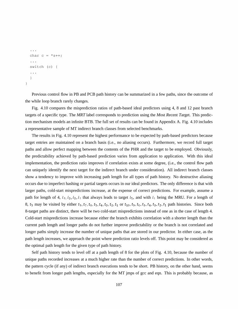
char c = *s++;

...

switch (c) {

...

}

}

Previous control flow in PB and PCB path history can be summarized in a few paths, since the outcome of

the while loop branch rarely changes.

Fig. 4.10 compares the misprediction ratios of path-based ideal predictors using 4, 8 and 12 past branch

targets of a specific type. TheMRT label corresponds to prediction using theMostRecentTarget. This predic-

tion mechanism models an infinite BTB. The full set of resultscan be found in Appendix A. Fig. 4.10 includes

a representative sample of MT indirect branch classes from selected benchmarks.

The results in Fig. 4.10 represent the highest performance to be expected by path-based predictors because

target entries are maintained on a branch basis (i.e., no aliasing occurs). Furthermore, we record full target

paths and allow perfect mapping between the contents of the PHR and the target to be employed. Obviously,

the predictability achieved by path-based prediction varies from application to application. With this ideal

implementation, the prediction ratio improves if correlation exists at some degree, (i.e., the control flow path

can uniquely identify the next target for the indirect branch under consideration). All indirect branch classes

show a tendency to improve with increasing path length for all types of path history. No destructive aliasing

occurs due to imperfect hashing or partial targets occurs inour ideal predictors. The only difference is that with

larger paths, cold-start mispredictions increase, at the expense of correct predictions. For example, assume a

path for length of 4,t4; t3; t2; t1 that always leads to targett5, and witht1 being the MRU. For a length of

8, t5 may be visited by eithert8; t7; t6; t5; t4; t3; t2; t1 or t10; t9; t6; t5; t4; t3; t2; t1 path histories. Since both

8-target paths are distinct, there will be two cold-start mispredictions instead of one as in the case of length 4.

Cold-start mispredictions increase because either the branch exhibits correlation with a shorter length than the

current path length and longer paths do not further improve predictability or the branch is not correlated and

longer paths simply increase the number of unique paths thatare stored in our predictor. In either case, as the

path length increases, we approach the point where prediction ratio levels off. This point may be considered as

the optimal path length for the given type of path history.

Self path history tends to level off at a path length of 8 for the plots of Fig. 4.10, because the number of

unique paths recorded increases at a much higher rate than the number of correct predictions. In other words,

the pattern cycle (if any) of indirect branch executions tends to be short. PB history, on the other hand, seems

to benefit from longer path lengths, especially for the MT jmps of gcc and eqn. This is probably because, as

107

4 5 6 7 8 9 10 11 1230

40

50

60

70

80

90

100gcc : MT jmp predictability and path correlation length

Pe

rce

nta

ge

(%

)

Path length

MRTSelfPBPIBPCB

4 5 6 7 8 9 10 11 1298.4

98.6

98.8

99

99.2

99.4

99.6

99.8

100edg : FP jsr predictability and path correlation length

Pe

rce

nta

ge

(%

)

Path length

MRTSelfPBPIBPCB

4 5 6 7 8 9 10 11 1255

60

65

70

75

80

85

90

95eqn : MT jmp predictability and path correlation length

Pe

rce

nta

ge

(%

)

Path length

MRTSelfPBPIBPCB

4 5 6 7 8 9 10 11 1279

80

81

82

83

84

85

86

87

88troff : VF jsr predictability and path correlation length

Pe

rce

nta

ge

(%

)

Path length

MRTSelfPBPIBPCB

Figure 4.10: Misprediction ratios of MT indirect branch classes with path correlation lengths of 0, 4, 8 and 12.

more targets are inserted in the PHR, patterns of switch-based jmps are gradually recorded and predictability

improves. The same phenomenon is seen with PCB history, mainly because it is a subset of PB history. If we

look at the absolute prediction ratios, Self path history has a better prediction ratio for the MT jmp branches

compared to PCB or PB, and a poorer accuracy when it comes to indirect calls (VF and FP jsr). We investigated

this issue by looking at the source code usage of switches in gcc and eqn. The following example is taken from

gcc.

mark_set_resources(rtx x, ...) {

...

restart:

code = x->code;

switch(code) {

...

case INSN:

108

...

x = x->fld[3].rtx;

if (...) goto restart;

...

case SET:

mark_set_resources(x->fld[0].rtx,...);

...

case CALL_INSN:

for (...) {

mark_set_resources((x->fld[3].rtx)->fld[0].rtx,...);

...

}

...

}

...

}

The switch statement is executed via either the goto statement or via loop-nested recursive invocations of

proceduremark set resources. Additional examples, not shown here, revealed recursive calls inside two

nested loops. Note that the next target of the switch is determined by a field extracted from the pointerx, which

is passed as a parameter. The value ofx is assigned inside the for loop or when visiting some of the individual

case statements. Therefore, this particular MT jmp branch requires previous self history and/or past history

from procedure calls.

On the other hand, PB and PCB history need longer path lengthsto record the pattern of the MT jmp targets,

since conditional branches (such as those from the for loop)interfere. This is not the case with PIB history,

where performance is better. With PIB history, we record alltargets coming from the switch statement as we

do in Self history. In addition to switches, we also store indirect procedure calls and returns. This seems to

be beneficial for the above example, where recursive invocations are interleaved with Self history and improve

predictability. In eqn, the activity of past procedure calls is not instrumental in accurately predicting the next

target for a switch statement. Frequently executed switch statements are found to be nested. Self path history

does not interleave targets from different branches, and thus, fails to reach the accuracy of PIB history. The

increased number of cold-start mispredictions for the Selfpath history predictor also verifies this weakness.

If we look at FP jsr branches, we see that this does not hold. Self path history does not produce with good

prediction ratios, simply because indirect calls do not tend to access functions in patterns. In general, PIB

history performs best across different path lengths. Notice though that in edg, the prediction ratio for FP jsr

calls with PIB history drops with increasing path lengths. The rather unpredictable behavior of the remaining

types of path history signifies that the optimal type of control flow depends on the programming style. For

109

example, one FP jsr in edg calls a termination function that decides on the pruning of Intermediate Language

(IL) entries. This function pointer points to different termination functions at different parts of the program.

Setting the terminating function pointer is either controlled by the outcome of a conditional or set to NULL.

Long PB and PCB history are the best methods for predicting this branch. Another example is when edg uses

function pointers to traverse the IL. Nested switch statements specialize the traversal based on the type of the IL

module, and for each case, the pointer is cast to a function that relates to the IL construct currently investigated.

In certain cases, extra conditional branches are used to further extend the IL classification scheme.

Recording the return instructions and the switch-based targets (PIB history), improves the process of distin-

guishing between the different targets of the pointer. Considering conditional branches, as we do in PB history,

causes some pollution, but after a certain path length, PB history seems to improve predictability. PCB history

also helps since the outcome of conditional branches differentiate between some of the cases. Sample source

code for the example just discussed follows.

case iek_scope:

...

if (walk_remap_func != NULL) {

ptr->next = (a_scope_ptr) walk_remap_func((char *)(ptr->next),(iek_scope))

}

In Fig. 4.11, we present the breakdown of mispredictions into cold-start and conflict. With edg, more than

55% of mispredictions are cold-start, independent of history type. PIB history reaches 100% with just 8 targets.

That means that either the existing path history is adequatefor predicting the next target, or that FP jsr branches

are strongly monomorphic and so increasing path length doesnot really contribute to their predictability. Given

the prediction ratios in Fig. 4.10, either justification seems reasonable.

VF jsr branches tend to be more predictable using previous control flow history, although Self history is

still inadequate in most cases. In troff, a frequently detected example of using polymorphism is a linked list

traversal via a for or while loop. The list consists of objects, and on every iteration, a virtual function is called.

Based on the run-time type of the object, a different function implementation can be invoked. Two examples

from troff are shown below where procedurestprint andspread space are virtual.

while (n != 0) {

n->tprint(this);

n = n->next;

}

for (node *tem = n; tem; tem = tem->next)

tem->spread_space(&nspaces,&desired_space);

110

If the linked list has not been modified between different traversals, or within the same traversal, Self his-

tory can detect patterns of virtual function call targets very quickly. However, the path length is fixed and

can not scale with the period of target patterns, since the linked list can become arbitrarily large or small. A

single insertion/deletion can destroy the links between patterns and targets established over time. On the other

hand, PIB history performs the best since both indirect calls and returns fill the PHR. This seems to be a bet-

ter adaptation mechanism, since for a fixed path length, the PIB records less history than the Self PHR (the

call/return pair identify the virtual function implementation the same way the call does). Pollution for interven-

ing calls/returns/switches does not seem to be a problem, since in C++, a large number of member functions

(such astprint or spread space of the examples above) are either leaf functions or rarely call another pro-

cedure (the rarely invoked callees usually implement error-detecting functionality). If they frequently invoke

another procedure they tend to call the same procedure everytime they are invoked. If the branch is monomor-

phic, the smaller number of unique paths recorded by PIB history also helps. The effectiveness of PB and PCB

history depends on intervening conditional branches (suchas the backward branch of the for/while loop). PCB

history is not effective if only loop branches are recorded.Loop branch history does not expose anything about

the polymorphic call nature. PB history combines all branches and gives results that lie between those of PCB

and PIB history.

A more complicated scenario in troff occurs when a recursivevirtual function A, invokes some other virtual

function B. The recursive call of A to A modifies the type of theobject pointed to by the pointer making the

call to B. On the other hand, B calls different implementations of A based on the type of its parameter, which

is an pointer to an object. We illustrate this scenario with the following source code from troff.

node *kern_pair_node::merge_glyph_node(glyph_node *gn) {

node *nd = n2->merge_glyph_node(gn); /* n1, n2 = static pointers to object */

if (nd == 0) return 0;

n2 = nd;

nd = n2->merge_self(n1);

if (nd) {

nd->next = next;

n1 = 0; n2 = 0; delete this;

return(nd);

}

return(this);

}

node *glyph_node::merge_self(node *nd) {

return(nd->merge_glyph_node(this));

111

}

Recursion is terminated by invoking different implementations of proceduremerge glyph node (not shown

here). The indirect call inside proceduremerge self is correlated with other indirect branches (PIB history

with call/returns from different implementations ofmerge glyph node). Recording the previous targets of the

indirect call does not provide us with any added accuracy. PBhistory is successful since conditional branches

are used in the remaining implementations ofmerge glyph node to control the flow. PCB history is not as

successful as PIB or PB since conditional branches only do not capture the whole picture.

Fig. 4.11 shows cold start mispredictions for the same benchmarks, for the branch classes presented in Fig.

4.10. The cold start misprediction ratio is listed as a percentage of the total misprediction ratio. As path length

increases, the cold-start ratio increases since more unique paths are recorded. The cold-start ratios foretell the

effectiveness of prediction via path-based correlation. If a large number of mispredictions are cold-start misses

then it is highly likely that branches of this class are not correlated via a specified type of path history (edg -

FP jsr - all types of history, gcc - MT jmp - (PCB, PB)). It couldalso mean that path length is inadequate for

capturing existing correlation, but this can be verified by looking at the ratio of cold-start mispredictions as the

path length increases. If the cold-start ratio remains approximately the same as we increase the path length, and

the misprediction ratio drops, then branches of this class tend to be correlated with longer path lengths (troff -

VF jsr - PIB, PCB, PB). If the cold start ratio increases with increasing path length, and the misprediction ratio

drops, then we approach the point of optimal path length (gcc- MT jmp - (PIB, Self), eqn - MT jmp - PIB).

Beyond that point, no correlation exists or can be exploited. The full set of results is in Appendix B.

4.4 Load-based Characterization

In this section we study the run-time behavior of the load instructions issued to support the statements imple-

mented by indirect branches. We label these loadsib-loads. The exact number and functionality of ib-loads

can be found in subsections 4.2.1, 4.2.2 and 4.2.3. We have developed a data-flow and control-flow analysis

framework to detect these loads using the ATOM tracing tool [60]. Our analysis is intraprocedural, since it is

highly unlikely that these loads, being true dependent upontheir associated indirect branches, will be moved

away from the procedure where the branch is issued. The only case where ib-loads may lie in a different pro-

cedure, is that of the FP jsr calls. A function pointer may be aparameter, a return value from a procedure call,

a local or a global variable. A number of memory dereferencespreceding the loading of the function pointer

may be located at the caller site.

As the gap between memory access time and microprocessor clock cycle continues to grow, the need for

112

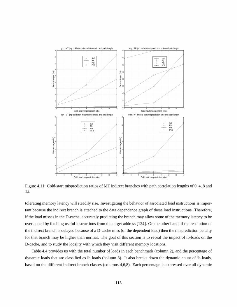
4 5 6 7 8 9 10 11 120

5

10

15

20

25

30

35

40

45gcc : MT jmp cold start misprediction ratio and path length

Pe

rce

nta

ge

(%

)

Cold start misprediction ratio

SelfPBPIBPCB

4 5 6 7 8 9 10 11 1220

30

40

50

60

70

80

90

100edg : FP jsr cold start misprediction ratio and path length

Pe

rce

nta

ge

(%

)


SelfPBPIBPCB

4 5 6 7 8 9 10 11 120

5

10

15

20

25

30

35eqn : MT jmp cold start misprediction ratio and path length

Pe

rce

nta

ge

(%

)


SelfPBPIBPCB

4 5 6 7 8 9 10 11 120

5

10

15

20

25

30

35troff : VF jsr cold start misprediction ratio and path length

Pe

rce

nta

ge

(%

)


SelfPBPIBPCB

Figure 4.11: Cold-start misprediction ratios of MT indirect branches with path correlation lengths of 0, 4, 8 and12.

tolerating memory latency will steadily rise. Investigating the behavior of associated load instructions is impor-

tant because the indirect branch is attached to the data dependence graph of those load instructions. Therefore,

if the load misses in the D-cache, accurately predicting thebranch may allow some of the memory latency to be

overlapped by fetching useful instructions from the targetaddress [124]. On the other hand, if the resolution of

the indirect branch is delayed because of a D-cache miss (of the dependent load) then the misprediction penalty

for that branch may be higher than normal. The goal of this section is to reveal the impact of ib-loads on the

D-cache, and to study the locality with which they visit different memory locations.

Table 4.4 provides us with the total number of loads in each benchmark (column 2), and the percentage of

dynamic loads that are classified as ib-loads (column 3). It also breaks down the dynamic count of ib-loads,

based on the different indirect branch classes (columns 4,6,8). Each percentage is expressed over all dynamic

113

Program loads ib-loads VF jsr FP jsr MT jmpin M Dyn % Dyn % targets Dyn % targets Dyn % targets

perl 688 5.0 0 0 1.2 720 3.8 5.0gcc 307 3.7 0 0 0.2 50.1 3.5 5.7edg 77 6.3 0 0 3.6 97.9 2.7 4.9gs 41 9.1 0 0 3.4 5.8 5.7 4.3troff 33 6.9 5.6 33.6 0.5 1.7 0.8 3.3eqn 12 5.0 2.5 59.7 0.9 1.0 1.5 6.0ixx 12 10.1 7.2 14.1 1.8 4.8 1.1 8.7eon 393 10.2 7.5 5.5 2.7 1.0 0.0 1.3porky 517 3.6 0.2 32.6 3.4 8.4 0 0bore 827 3.9 0.2 43.2 3.8 6.5 0 0lcom 48 7.2 4.6 252 0.1 1.6 2.5 10.4

Table 4.4: Statistics of ib-load instructions: number of executed loads (column 2), percentage of dynamic ib-loads over all dynamic loads (column 3), percentage of ib-loads due to VF jsr, FP jsr and MT jmp over alldynamic loads (columns 4, 6 and 8) and average number of targets per ib-load accompanying a VF jsr, FP jsror MT jmp (columns 5, 7 and 9).

loads. For each branch class, we also list the average numberof load addresses or load targets (columns 5,7,9).

The dynamic frequency of ib-loads, relative to all loads, ranges from 3 to 10%. These numbers provide

us with a lower bound, since not all ib-loads are determined intraprocedurally. The average number of targets

accessed by an ib-load of a polymorphic call heavily varies,since one of these loads accesses the object making

the call. These objects are often dynamically allocated entities, that may be allocated/deallocated multiple

times during the execution of the program. The second type ofload for a VF jsr accesses an entry in the VFT.

Although VFTs are usually not relocated in the memory address space, these loads may accessdifferentVFTs

if the type of the object changes. They access fewer targets than other types of ib-loads, but rarely exhibit a

monomorphic nature.

Ib-loads, supporting function pointer-based calls, have arather bimodal nature. They either access function

pointers from one or two locations, or they spread out their references over a large set. The later may occur

when the pointer traverses arrays of function pointers, while the former can occur with GOT-based calls. Ib-

loads supporting the functionality of MT jmp branches traverse the JTBL associated with the switch statement.

The JTBLs are usually stored in the read-only data area of thetext segment, and are not relocated. The ib-loads

associated with JTBLs present higher variability than the branch itself, since different JTBL entries may point

to the same case statement (the JTBL is sparse).

Fig. 4.12 displays the dynamic count of monomorphic, polymorphic and megamorphic ib-loads. The

114

breakdown of their dynamic counts comes into agreement withthe results in Table 4.4. Predicting the targets

of VF jsr and certain FP jsr ib-loads will be a challenge for traditional value/load address predictors, such as a

last valuepredictor. Even with more sophisticated two-level adaptive structures [123], the misprediction ratio

may not be satisfactory. On the other hand, the loads due to MTjmp branches are easier to predict, since more

than 50% of them are monomorphic.

0 20 40 60 80 100

lcom

bore

porky

eon

ixx

eqn

troff

VF jsr: ibload classification based on number of visited targets

Percentage (%)

MonoPolyMega

0 20 40 60 80 100

lcom

bore

porky

eon

ixx

eqn

troff

gs

edg

gcc

perl

FP jsr: ibload classification based on number of visited targets

Percentage (%)

MonoPolyMega

0 20 40 60 80 100

lcom

bore

porky

eon

ixx

eqn

troff

gs

edg

gcc

perl

MT jmp: ibload classification based on number of visited targets

Percentage (%)

MonoPolyMega

Figure 4.12: Dynamic counts of Monomorphic, Polymorphic and Megamorphic ib-loads associated with VFjsr, FP jsr and MT jmp branches.

On the left side of Fig. 4.13 we present the dynamic count of ib-loads broken down based on the indirect

branch type. There are two bars, one for committed and another for executed ib-loads. These results are

collected using the SimpleScalar simulator. The machine configuration was described in chapter 2. No explicit

indirect branch prediction scheme has been used. Each countis expressed as a percentage computed over all

committed/executed loads in the program. The plot on the right side, uses the same machine configuration to

115

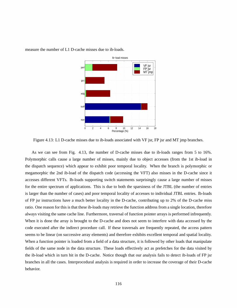
measure the number of L1 D-cache misses due to ib-loads.

0 2 4 6 8 10 12 14 16 18

eqn

troff

edg

gcc

perl

Ib−load misses

Percentage (%)

VF jsrFP jsrMT jmp

Figure 4.13: L1 D-cache misses due to ib-loads associated with VF jsr, FP jsr and MT jmp branches.

As we can see from Fig. 4.13, the number of D-cache misses due to ib-loads ranges from 5 to 16%.

Polymorphic calls cause a large number of misses, mainly dueto object accesses (from the 1st ib-load in

the dispatch sequence) which appear to exhibit poor temporal locality. When the branch is polymorphic or

megamorphic the 2nd ib-load of the dispatch code (accessingthe VFT) also misses in the D-cache since it

accesses different VFTs. Ib-loads supporting switch statements surprisingly cause a large number of misses

for the entire spectrum of applications. This is due to both the sparsiness of the JTBL (the number of entries

is larger than the number of cases) and poor temporal locality of accesses to individual JTBL entries. Ib-loads

of FP jsr instructions have a much better locality in the D-cache, contributing up to 2% of the D-cache miss

ratio. One reason for this is that these ib-loads may retrieve the function address from a single location, therefore

always visiting the same cache line. Furthermore, traversal of function pointer arrays is performed infrequently.

When it is done the array is brought to the D-cache and does notseem to interfere with data accessed by the

code executed after the indirect procedure call. If these traversals are frequently repeated, the access pattern

seems to be linear (on successive array elements) and therefore exhibits excellent temporal and spatial locality.

When a function pointer is loaded from a field of a data structure, it is followed by other loads that manipulate

fields of the same node in the data structure. These loads effectively act as prefetches for the data visited by

the ib-load which in turn hit in the D-cache. Notice though that our analysis fails to detect ib-loads of FP jsr

branches in all the cases. Interprocedural analysis is required in order to increase the coverage of their D-cache

behavior.

116

4.5 Summary

We have presented a characterization study of indirect branches for a set of C and C++ benchmarks. Indirect

branches were partitioned in classes based on their source code usage and their predictability, target locality

and entropy has been studied using ideal predictors. The idea was to examine the potential of the last-value

and path-based prediction algorithms without consideringside-effects such as finite table size and aliasing. We

have also studied the behavior of loads that are true-dependent on indirect branches.

Results showed that different branches exhibit varying behavior. This behavior depends on the program-

ming style and the input of the application. As expected, last-value prediction worked accurately only on

monomorphic and low entropy branches while path-based prediction’s accuracy largely varied based on the

path length and the type of path history. In general, PIB history was found to be the best type of path history

for our benchmark suite. The optimal path length varied depending on the branch class and the type of path

history.

117

Chapter 5

Indirect Branch Prediction Mechanisms

A large number of indirect branches is found in applicationsdeveloped using the OOP model. The main reason

is that these branches implement polymorphic calls. Depending on the programming language, the dynamic

frequency of those branches can be substantial. On the otherhand, indirect branches prevent microprocessors

from exploiting ILP via control speculation because they always disrupt the sequential instruction flow.

This chapter presents a set of indirect branch prediction schemes that utilize past branch outcome or target

history and/or load latency information to reduce the penalty associated with indirect branches. First, we intro-

duce the Prediction by Partial Matching (PPM) algorithm as it applies to the field of indirect branch prediction.

The PPM algorithm has been originally proposed for text/data compression and has also been considered for

conditional branch prediction. We describe one possible implementation of a PPM-based indirect branch pre-

dictor and evaluate its performance in the context of an out-of-order superscalar microprocessor. In addition,

we show how this design can be enhanced with dynamic selection of path correlation type on an individual

indirect branch basis. The second part of the chapter is associated with a preliminary study on the effects of an

alternative replacement policy for indirect branch predictors. We explore two options. The first one records the

latency tolerance of ib-loads, and the second, the temporallocality of indirect branches. We also demonstrate

one way of combining these two techniques.

5.1 Related Work

Past work on indirect branch prediction originally can be tracked back to [58, 125, 126], where the foundations

behind theBranch Target Buffer(BTB) design were established. A BTB is a cache-like structure which stores

targets of previously seen branches. In the context of valueprediction, the simplest implementation of a BTB

acts like a last-value predictor. It can replace logic used to compute the target whenever a branch is predicted

118

to be taken in order to provide prediction at an earlier stageof the pipeline. In practice, it has been used to

predict the targets of all branches. A BTB most often allocates a single entry for a branch and keeps its most

recent target in that entry. Therefore, it can be very effective for conditional branches because these branches

transfer control flow to only one target. A BTB is ineffectivefor predicting indirect branches which can jump

to multiple targets. When the BTB mispredicts, the existingtarget address is replaced. A 2-bit counter can

be used to limit the update of the target address to only aftertwo consecutive mispredictions occur [120]. We

will refer to this configuration asBTB2b. The BTB2b can produce a better branch prediction ratio for C++

applications by taking advantage of the locality exhibitedby the targets of virtual function calls.

In [35], Kaeli and Emma describe a mechanism which accurately predicts the targets of subroutine returns.

The mechanism is called aCall/Return Stack(RAS) and targets the prediction of subroutine returns by using

the inherent correlation between procedure calls and returns to pair up the correct target address with the

current return invocation. Due to its high prediction accuracy, a RAS is preferred when predicting the addresses

of return instructions. Several studies have concentratedon techniques of properly updating a RAS and/or

recovering its correct state during speculative executionmode [127, 128]. In our work, we will not address

issues related with the predictability of return instructions.

In [129], theCase Block Table(CBT) is proposed for predicting the next target of a switch statement. If the

compiler issues an indirect jump to implement the control transfer for a switch statement, the CBT becomes

essentially an indirect branch predictor. It uses the switch variable values to find the next target of a switch

statement. Since the switch variable value is an optimal predictor for a multi-way branch, the CBT accuracy

can be very high. The problem with the CBT is that the value of the switch variable is not always known at the

time the code for the switch statement reaches the instruction fetch stage of a multiple issue machine employing

speculative execution [130].

In [109], Driesen and Holzle propose using two-level adaptive predictors for indirect branches similar in

structure to the conditional branch predictor originally proposed in [131]. The first level consists of one global,

or multiple (per branch) history registers that record partial previous targets of branches allowing path-based

correlation to be exploited. Since every register records previous path history, it is called aPath History Register

(PHR). The number of targets recorded in the PHR is called thepath length. The second level consists of a table

where each entry consists of a target and a 2-bit counter thatcontrols the replacement of the target. Each entry

can optionally include a valid bit, a tag, a confidence counter, etc. The 2nd level has been traditionally named

asPattern History Table(PHT) and is usually indexed with the branch address (PC). Analternative hashing

scheme exclusive-ORs the branch address and the PHR contents (gshare). In [109, 108], the authors proposed

grouping or interleaving bits of the PHR and the branch’s address to index the PHT.

Driesen and Holzle explored a large number of ideal two-level predictor configurations. They obtained

119

the best prediction accuracy using the GAp structure (Global PHR, Per-address PHT configuration) for their

set of benchmarks. In more recent work [108], Driesen and Holzle explored realistic designs, varying the

path length the size, the associativity and the hashing function used for the PHT. They also proposed a hybrid

design, namely a dual-path predictor, where each componentis a two-level predictor. The two components

differ in path length. A set of confidence counters, placed inthe PHTs (and not in a separate array, as originally

proposed in [107]), was used to select which component wouldmake a prediction. Their findings suggest that

the best dual path predictor should have components containing both a short and a long path length, because

most indirect branches tend to be either short or long lengthcorrelated.

Chang et al. proposed using a family of two-level predictors[130], named the Target Cache (TC), with a

structure similar to the two-level adaptive scheme described in [109]. The novel feature of the TC predictor is

that the PHR records partial targets from a selected group ofbranches. In [130], the TC selects branches based

on their opcode, leading to the following types of path history : Per Branch path history (PB) from the targets

of all branches, Per Conditional Branch (PCB) path history from the targets of only conditional branches, Per

Indirect Jump (PIJ) path history from the targets of indirect jumps and Per Procedure Call/Return (PPCR) path

history from the targets of procedure call and return instructions. Each TC configuration utilizes PHR(s) from

only one group of branches. The different contents recordedin the PHR allows variance in the type of path

correlation across multiple TC configurations. The simulation results clearly show the dependence of indirect

branch predictability on the type of path-based correlation.

Driesen and Holzle in [132] proposed using a filter along witha main component to construct a hybrid

indirect branch predictor, namely the Cascaded predictor.The authors present a path-based predictor (hybrid

dual-path) as the main component and a BTB-like structure asa filter. The latter is used to dynamically classify

and predict easily predictable branches while the former predicts the remaining branches. By filtering out the

easy to predict branches in the main component, phenomena such as aliasing and capacity mispredictions due

to path history can be significantly reduced.

The BTB structure of the filter permits the prediction ofmonomorphic1 andlow entropybranches2. Two

different protocols were proposed to determine when and howprediction would be made by a filter: i) strict

and ii) leaky. A strict filter disallows new entries to be inserted into the main component when the branch is

not found in the filter and allows the creation of an entry in the main component when a branch is mispredicted

by the filter. In order to distinguish between a miss and a misprediction, the strict filter must maintain tags. A

leaky filter allows entries to be created in both components on a branch miss. Only correctly predicted branches

(by the filter) do not update the main component. Since a leakyfilter does not distinguish between a branch1A branch is monomorphic when it mostly accesses one target.2A branch has low entropy when its target changes infrequently.

120

miss and a misprediction no tags are necessary in its implementation. The authors found that a leaky filter led

to overall lower misprediction ratios than a strict filter [132].

In [133], Stark et.al. proposed a branch prediction scheme that exploits profile-based variable path length

correlation for both conditional and indirect branches. Intheir implementation, a set of hashing functions

combining a variable number of targets, is implemented in hardware. A PHR records the N most recently

encountered branch targets and feeds them to hashing function hardware. The latter generates a set of indices

from which the target is selected via a multiplexer, controlled by information bits (called a hashing function

index). These bits are set after extensive profiling of all branches is performed. The compiler/linker is respon-

sible for communicating the hashing function indices to thehardware. The solution described in [133] uses the

Instruction Set Architecture (ISA). The displacement fieldof the Alpha AXP indirect branches is used to store

these indices. A table, indexed by the branch’s address, is used to store these bits in hardware. The profiling

step guarantees that the hashing function selected for eachbranch is optimally tuned in terms of misprediction

ratio. The index that goes through the multiplexer drives a 2nd-level table (similar to a PHT) that actually

makes the prediction. Stark’s scheme can be used to predict both conditional and indirect branches.

Recently, Roth et.al. suggested using a dataflow engine, to complement conventional path-based predic-

tors, in order to improve the predictability of virtual function calls [134]. Their solution detects the dispatch

code sequence implementing a virtual function call. The engine records the corresponding dependencies and

launches computations via a dataflow engine, in the order object references are made, in an attempt to predict

the next target before the indirect call is executed. The authors also propose the use of a lookahead scheme,

where stride-based address prediction can assist the launching of computations, early enough before their as-

sociated object references are detected in the dynamic instruction stream. Simulation results showed that their

dependence-based prediction scheme can improve the misprediction ratio of a set-associative BTB and a two-

level path-based predictor.

5.2 Data Compression Algorithms and Branch Prediction

The primary goal of data compression is to replace an original data sequence with another that has fewer

data elements. Modern data compression techniques try to use fewer bits to represent frequent symbols, thus

reducing the overall size of data. The text/data compression algorithm usually defines a probabilistic model

that is used to predict the next symbol with high accuracy. The ability of a compression algorithm to accurately

predict stems from the close relation between compression and prediction: a sequence that is compressed well is

easy to predict. On the other hand, a random sequence is both non-compressible and unpredictable [135, 136].

121

Since accurately predicting branches is of great importance for modern microprocessors, applying compres-

sion techniques to branch prediction appears to be an attractive solution. In this section we present two com-

pression algorithms as they apply to branch prediction: i) thePrediction by Partial Matching(PPM) [137, 138]

algorithm and ii) theContext Weight Tree(CWT) [139].

The CWT method builds a binary tree of lengthd based on past branch outcomes. Every tree node is

assigned a context, which is the unique bit sequence generated if we traverse the tree from the root to the

node. The root always has a null context. A node is created only if its context has been seen in past branch

history. Given a set of past branch outcomesS, the set of bits immediately succeeding the context of a node

in S is called the subsequence of the node. The tree is called a context weight tree (CWT) because every

node is assigned a weighted probability (Pw) which is derived from the conditional probability of finding the

subsequence associated with the node (Pe) and the weighted probabilities of the node’s children. Theweighted

probability of the root weights the probabilities induced by all possible complete subtrees. In order to predict

the next branch outcome we assume that is taken (1), append the new outcome in the branch history, recompute

the weighted probabilities of all affected nodes in the pathand find the ratio of the new over the old weighted

probability of the CWT’s root node. A randomized predictor is used to make the final decision as follows:� if ratio > 0:5 + "! prediction= 1 (branch is taken).� if ratio < 0:5 � "! prediction= 0 (branch is non-taken).� else prediction= 1 with probability�(P )where" = 1pT andT is the branch history length.

The authors in [140] also discuss variations of the CWT algorithm, where they add bits from the branch

address in the past branch history, to further increase the levels of the context tree. The original CWT con-

struction algorithm assumes that a complete context tree isbuilt, where the total number of nodes is determined

only by the branch history. This version of the algorithm is called static. By setting a limit on the number of

nodes (and levels), Federovksy et.al. create an adaptive version of the CWT algorithm. They limit the number

of CWT nodes by deallocating nodes that no longer carry information within the branch history window. The

number of CWT levels is controlled by not limiting the extension of a particular context at the leaf node when

a threshold is reached. The original CWT algorithm carries the following per node information:� a count of 1s (denoted byb) and 0s (denoted bya) of the node’s context,� the probability estimate (Pe) of the node’s subsequence, and� the weighted probability (Pw) of the node.

122

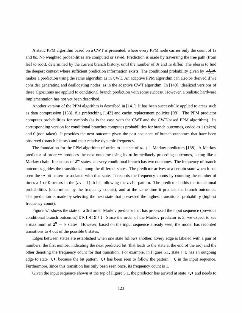
A static PPM algorithm based on a CWT is presented, where every PPM node carries only the count of 1s

and 0s. No weighted probabilities are computed or saved. Prediction is made by traversing the tree path (from

leaf to root), determined by the current branch history, until the number of 0s and 1s differ. The idea is to find

the deepest context where sufficient prediction information exists. The conditional probability given byb+0:5a+b+1makes a prediction using the same algorithm as in CWT. An adaptive PPM algorithm can also be derived if we

consider generating and deallocating nodes, as in the adaptive CWT algorithm. In [140], idealized versions of

these algorithms are applied to conditional branch prediction with some success. However, a realistic hardware

implementation has not yet been described.

Another version of the PPM algorithm is described in [141]. It has been successfully applied to areas such

as data compression [138], file prefetching [142] and cache replacement policies [98]. The PPM predictor

computes probabilities for symbols (as is the case with the CWT and the CWT-based PPM algorithm). Its

corresponding version for conditional branches computes probabilities for branch outcomes, coded as 1 (taken)

and 0 (non-taken). It provides the next outcome given the past sequence of branch outcomes that have been

observed (branch history) and their relative dynamic frequency.

The foundation for the PPM algorithm of orderm is a set ofm + 1 Markov predictors [138]. A Markov

predictor of orderm produces the next outcome using itsm immediately preceding outcomes, acting like a

Markov chain. It consists of2m states, as every conditional branch has two outcomes. The frequency of branch

outcomes guides the transitions among the different states. The predictor arrives at a certain state when it has

seen them-bit pattern associated with that state. It records the frequency counts by counting the number of

times a 1 or 0 occurs in the (m + 1)-th bit following them-bit pattern. The predictor builds the transitional

probabilities (determined by the frequency counts), and atthe same time it predicts the branch outcomes.

The prediction is made by selecting the next state that possessed the highest transitional probability (highest

frequency count).

Figure 5.1 shows the state of a 3rd order Markov predictor that has processed the input sequence (previous

conditional branch outcomes)01010110101. Since the order of the Markov predictor is 3, we expect to see

a maximum of23 = 8 states. However, based on the input sequence already seen, the model has recorded

transitions to 4 out of the possible 8 states.

Edges between states are established when one state followsanother. Every edge is labeled with a pair of

numbers, the first number indicating the next predicted bit (that leads to the state at the end of the arc) and the

other denoting the frequency count for that transition. Forexample, in Figure 5.1, state110 has an outgoing

edge to state101, because the bit pattern101 has been seen to follow the pattern110 in the input sequence.

Furthermore, since this transition has only been seen once,its frequency count is 1.

Given the input sequence shown at the top of Figure 5.1, the predictor has arrived at state101 and needs to

123

0 1 0

1 0 10 1 1

1 1 0

Input sequence : 0 1 0 1 0 1 1 0 1 0 1 ?

0 1 0 1 0 1 1 0 1 0 1 ?

Last 3 bits

0 1 0 1 0 1 1 0 1 0 1 ?

Last 2 bits

3rd order Markov predictor

2nd order Markov predictor

0 1 0 1 0 1 1 0 1 0 1 ?

Last 1 bit

1st order Markov predictor

if not found

if not found

if not found

0th order Markov predictor

1/3

0/2

1/1

1/1

1/1

Figure 5.1: Prediction algorithm for a 4th order PPM predictor as it applies to conditional branch prediction.

predict the value of the next bit. Pattern010 has followed101 twice, while pattern011 has followed101 only

once. Therefore, the next state should be010 and the predicted value of the bit will be 0.

As mentioned above, a PPM predictor of orderm consists of a set ofm + 1 Markov predictors. At step 1

themth order Markov predictor is searched for a pattern, formed by them immediately preceding bits in the

input sequence. If a match is found (meaning that the state associated with the pattern has at least one outgoing

edge), a prediction is made. If the Markov predictor fails tofind the pattern (meaning that the state associated

with the pattern has no outgoing edges), it looks into the next lower order Markov predictor for a pattern formed

by them � 1 immediately preceding bits. This process is continued until a prediction is made. Notice that a

0th order Markov predictor will always make a prediction based on the relative frequency of 0s and 1s in the

input sequence. Returning to Figure 5.1, the PPM algorithm will first search for the101 bit pattern in the 3rd

order Markov predictor, then it will look for pattern01 in the 2nd order Markov predictor, etc.

The update step of the frequency counts, across different order Markov models in the PPM algorithm, varies.

Throughout this thesis, we will use anupdate exclusion policy[141]. This protocol excludes all predictors

with a lower order (i.e., lower than the one that actually makes the prediction) from being updated. Only the

predictor that makes the decision, and the predictors with ahigher order, are updated. Implementations of the

PPM algorithm are discussed in the following section.

124

5.3 PPM-based Indirect Branch Predictors

In [141], Chen et al. discussed how a PPM predictor of orderm can be seen as a set ofm+1 two-level adaptive

predictors, thus providing us with a theoretical basis for supporting the accuracy of the later. The key idea

is that a Markov model, as shown at the top of Figure 5.1, is successfully emulated by a two-level adaptive

predictor. Them-bit input sequence is recorded in anm-bit history register (HR). The samem-bit sequence

can represent global or per branch history. The lookup of thepattern in the Markov model is simulated by the

lookup of the PHT using the contents of the HR. The 2-bit up/down saturating counters, provided on a PHT

entry basis, efficiently mimic the transitional probabilities. The states of the Markov model correspond to the

entries in the PHT on a 1-to-1 basis.

The PPM algorithm of orderm requiresm + 1 adaptive predictors; each of the adaptive predictors uses

an HR with a different length. Therefore, prediction is madeusing information from history lengths that

range fromm to 0. In other words, the PPM algorithm explores variable-length branch correlation. The 1st

order Markov predictor is simply a 1-bit history predictor (predicts the next branch outcome using its previous

outcome). The protocol of the PPM algorithm, as described above, assigns priority to long term correlation

(assuming thatm is large enough to reveal long-term branch correlation). This is because the PPM predictor

always uses the highest order Markov predictor that detectsthe pattern in the HR. Although this is necessary

when performing data compression, it may not be optimal whenapplied to branch prediction.

If we consider indirect branch prediction, a PPM predictor of orderm will again consist ofm+ 1 Markov

components, each one being indexed by a PHR of a different path length. The path length will range frommto 0, and therefore, the PPM predictor will also exploit variable path length correlation. The 1st order Markov

predictor simply uses the previous target to predict the next one. A PPM predictor for indirect branches can

utilize a global PHR to record past history. The only difference between ideal PPM models for conditional and

indirect branch prediction is that the total number of states for anmth-order Markov component is not2m butkm, wherek is the maximum number of valid targets in the program.

The goal in indirect branch prediction is to correctly predict the target of the branch. Since indirect branch

target address selection is not a binary decision, the application of the PPM algorithm is not straightforward.

Accurately describing path history requires storing 32-bit or 64-bit addresses, versus storing a single bit (i.e.,

the branch direction) in the case of conditional branches. Indexing a state in the Markov chain with the contents

of past history is not simple either. As was mentioned in Section 5.2, the maximum number of states in each

Markov component iskm. A PPM predictor would require enormous hardware resourcesin order to represent

all states of the Markov components.

Our solution is to use multiple BTB-like structures to implement the Markov chain states. These structures

125

are equivalent to PHT implementations in two-level predictors and we will refer to them as PHTs. We use a

PHR to record past history and a hashing function to form indices accessing the multiple PHTs. By limiting

the size of the PHTs, we are merging sets of the Markov chain states together. The final number of states after

merging is equal to the number of PHT entries. The hashing function proposed in [108, 130] uses a gshare

indexing scheme, where groups of bits from previous branches (conditional and/or indirect) are XOR’ed with

the PC to form the index. In our case, we use a modified version of the Select-Fold-Shift-XOR(SFSX) hashing

function described in [143].

. . . .101001001111011, 001011101000111, 111010001110001

10th Order PPM algorithm

Select

XOR XOR XOR

Most recent target

Fold

01000 11101 10010

XOR

1110001000

Shift

Xor

. . . . . . . .

.

.

.

.

.

. . . . .

. . . . . Index for 10th Order Markov predictor

Index for 9th Order Markov predictor

Select

Figure 5.2: Select-Fold-Shift-XOR-Select (SFSXS) indexing function as it applies to the contents of a PHR.

Figure 5.2 shows an example of how our new mapping function called Select-Fold-Shift-XOR-Select(SF-

SXS) forms an index from the path history. In this example, weshow a path length of 10 and a 10th order PPM

predictor, to illustrate how our indexing function works. The SFSXS mapping function selects the low-order 10

bits from targeti 3, folds the selected value into 5 bits which are left shifted by i bits and XOR’ed together with

the other values. Thej high order bits of the outcome form the index for thej-th order Markov predictor. An

alternative solution would select thej low order bits. From simulation results, we found little difference in the

misprediction ratios when comparing these two schemes, so we decided to use the scheme shown in Figure 5.2.

Another major problem when implementing the PPM algorithm for indirect branches is the selection of the

next target. The original Markov model requires multiple outgoing arcs from each state, keeping frequency

counts for each possible target. Obviously, this step does not involve a binary decision and can not be modeled3Since instructions are word-aligned we always ignore the last two bits of their addresses.

126

by a 2-bit counter. It requires storing multiple targets perPHT entry, along with their frequency counts, and a

majority voting mechanism to select the next target. Instead we store the most recently visited target and use it

to make a prediction.

Branch IdStructure

BranchAddress

Path History Register

target 3 target 2 target 1

target count tag

1st orderMarkov

Component(2 entries)

target count tag

3rd orderMarkov


target count tag

2nd orderMarkov


target count tag

0th orderMarkov

Component(1 entry)

Hashingfunction

Hashingfunction

Hashingfunction

predictedtarget

Indirect Branch detected

correct target

correct target

Branch Tag

Figure 5.3: Single-level access implementation of a 4th order PPM predictor. It uses a set of BTBs to implementthe Markov components. Each component is indexed with a variable number of targets, extracted from a singlePHR.

The complete design for a 4th order PPM predictor is shown in Figure 5.3. We assume an implementation of

the PPM predictor at the I-fetch stage of a processor employing speculative execution. The logical components

forming the predictor are a Branch Identification Unit (BIU), that indicates that an indirect branch is being

fetched. Most implementations assume two bits per entry to indicate whether the branch is conditional, a

return or indirect [144]. We also need a PHR that records partial targets from a predetermined branch stream.

To use the SFSXS mapping function, we will need to record 3 bits from each one of the last 3 targets. One

possible scheme is to record the targets of all indirect branches (PIB path history) in a single PHR. The boxes

labeled asHashing functionimplement the indexing scheme described in Figure 5.2. The Markov predictors

127

are basically BTB-like structures, where every entry includes the most recently accessed target, a tag, a 2-bit

up/down saturating counter for replacement and a valid bit.Using a 2-bit counter allows the target currently

found in an entry to be replaced only on two consecutive misses. Control logic selects one target from the

Markov components, according to the PPM protocol. Markov predictors can also be tagless. In the absence of

tags the only way to indicate a non-zero frequency count for astate of the Markov model is the valid bit. If we

allow an exclusive-update policy for the PPM predictor, most of the queries for a prediction will be directed

to the highest order Markov component, leading to an underutilization of the available resources. For detailed

simulation results on a tagless PPM predictor see [145]. Thesimulation results in this thesis will correspond to

tagged implementations only.

The PPM predictor works as follows. The BIU unit is interrogated using the branch address every time the

processor fetches instructions. At the same time, the PHR isused to generate the different indices and access

all the Markov predictors in parallel. If an indirect branch(other than a return) is detected in the instruction

stream, a tag comparison is made to examine if the entry in theMarkov component belongs to the branch

under consideration. The highest order Markov predictor “hit” provides the next target. If there is a miss,

no prediction is made (this event is classified as a misprediction in our experimental results). Under such a

scenario, after the branch is resolved, we only update the Markov component with the lowest 2-bit counter

value. If there is more than one Markov component with the same value, we update the highest order one.

Overall, the prediction step for the described PPM implementation requires a single level of table access, and

thus, the predictor can be characterized as 1-level.

The update step starts by shifting the actual target to the PHR, independent of whether we had a mispredic-

tion or not. By keeping a bit string ofm bits showing which component made a prediction, we can implement

an update exclusion policy [141]. This bit string can be associated with an indirect branch as it goes through the

different stages of the pipeline (one possible solution is to keep it as a separate entry in the reservation station

of the branch unit, along with the indirect branch’s information). For each component that needs to be updated,

we set the valid bit (if not set), and update the target (either speculatively or with the actual outcome). Timing

issues related to updating the target are not discussed in this work. Finally, we update the state of the counter

and the tag if the branch is being replaced in the PHT entry. All components can be updated in parallel.

Previous studies have shown that indirect branches have different characteristics than conditional branches,

especially when it comes to inter-branch correlation [130]. The experimental results in chapter 4 revealed that

most indirect branches were best correlated with either: 1)all previous branches or 2) with previous indirect

branches (PB or PIB correlated respectively). Therefore wehave combined the PPM predictor with a selection

scheme that dynamically chooses between two types of path-based correlation of the same length : 1) PB and

2) PIB path-based correlation. Since we wanted to characterize the correlation of every individual indirect

128

branch, we introduce a set of 2-bit up/down saturating counters in the BIU module. Based on the contents of

the associated counter, the predictor selects between the two PHRs. The new design is shown in Figure 5.4.

Branch IdStructure

BranchAddress

PIB Global Path History Register

target 3 target 2 target 1

predictedtarget

Indirect Branch detected, Branch tag

correct target

PB Global Path History Register

target 3 target 2 target 1correct target

PPM predictorMUX

correct target

SelectionCounter

Figure 5.4: PPM predictor with run-time selection of correlation type. Two PHRs are used to record pathhistory of PIB and PB type. Two-bit counters, kept on an indirect branch basis, select the PHR at run-time.

Notice that this version of the PPM predictor requires two serialized table accesses (one for the BIU and

one for the PPM predictor), and therefore it should be considered a 2-level predictor. Depending on the physical

implementation of the processor, the prediction may have tobe pipelined into two (or even more) phases. In

the first, the BIU structure is queried. If an indirect branchis found then one PHR is selected based on the the

associated 2-bit correlation counter. In the second phase,the selected PHR will then feed the multiplexer, and

the generated indices will index the Markov components of the main predictor body. The correlation selection

counters are updated at the same time with the Markov components. Every correlation selection counter follows

the state machine shown in Figure 5.5.

Each state of the counter is labeled with the contents of the counter and the PHR selected for that state.

The behavior of a branch can be characterized asStrongly PB correlated(state 00),Weakly PB correlated(state

01),Weakly PIB correlated(state 10) andStrongly PIB correlated(state 11). Dotted arcs represent a transition

triggered by a misprediction, while solid lines denote a change due to a correct prediction. The state machine

129

in Figure 5.5 models a normal 2-bit counter where the nature of correlation will change on two consecutive

mispredictions. All counters are initialized to theStrongly PIB correlatedmode.

00/PB

01/PB

10/PIB

11/PIB

Initial State

Selection CounterCorrect prediction

Misprediction

Figure 5.5: State machine of a 2-bit up/down saturating counter. The counter is used to select one of the twoavailable PHRs in a scheme that combines PPM prediction withrun-time selection of path history type.

5.4 Load Latency Tolerance and Indirect Branches

The penalty associated with indirect branches depends on the service time of their dependent load instructions.

As we have seen from chapter 4, at least one load instruction accompanies an indirect branch. Switch-based

jumps and virtual function calls have two loads. We renamed these loads asibloads in chapter 4. An indirect

branch is always truly dependent on one of the ibloads. If an ibload misses in the D-cache, then the time

to resolve the dependent indirect branch depends on the timethat load needs to be serviced by the memory

hierarchy. The ibload latency also depends on the level of memory hierarchy which will service the read

request. Since the time to resolve the branch depends on the ibload latency, the misprediction penalty of the

branch also depends on the load latency. The misprediction penalty can vary even more if a sequence of ibloads

lie on the same dependence chain. For example, a virtual function call is associated with two ibloads (see

subsection 4.2.2) which lie on the same dependence chain. A similar situation arises with switch-based jumps.

The number of ibloads that support pointer-based function calls depends on the source code. For example, if

the function pointer is a field in a complex data structure, then a series of dependent ibloads may be issued to

access the pointer. In general, the penalty differs among different indirect branches, as well as between dynamic

instances of the same branch.

130

Thus, indirect branches can be categorized based on their misprediction latency. The same argument has

been manifestated for conditional branches [124]. In this section we study a method that attempts to improve

the predictability of indirect branches by classifying them at run-time based on their misprediction latency. If

we know whether an ibload/ibload sequence will miss/hit in the D-cache at the indirect branch is predicted, then

we can use this decision to make a better prediction. We can also use this information when the IB predictor is

updated to assist future predictions.

The predictors we have discussed so far, try to exploit the run-time target patterns in an attempt to accurately

predict indirect branches. They do not consider the penaltyeach mispredicted branch will impose at run-

time. Incorporating information such as anticipation of a D-cache miss in such predictors must be carefully

designed. For example, we could modify the protocol of the cascade predictor as follows: the filter is assigned

with branches whose ibloads are anticipated to hit in the D-cache. The remaining branches are fed to a more

sophisticated component, since its prediction accuracy ishigher. By accurately predicting such branches, out-

of-order execution may be able to hide the load latency by fetching from the correct path. If we use a tagless

BTB as a leaky filter, filtering will target monomorphic branches. However, there is no obvious correlation

between such branches and the high hit ratio of their corresponding ibloads. Virtual function calls, which are

frequently monomorphic, may invoke the same function body most of the time, but not necessarily via the

same object or the same VFT. On the other hand, ibloads associated with switch-based jumps access the same

statically allocated data structure, the JTBL. This table is not relocatable, and its presence in the L1 D-cache

depends on how frequently the same static branch is called. The ibload behavior of function pointer-based calls

is even more complicated. If the function pointer is loaded from a GOT, then the target temporal locality of the

ibload is high, as long as the branch is executed closely in time. If the pointer is loaded from a data structure,

then the latency of ibloads heavily depends on the access pattern, the algorithm and the type of the structure

(tree, linked list, etc.). In addition to all of the above factors, there may exist distinct ibloads from different

control-flow paths leading to the same static branch.

Our approach is to modify the replacement policy of the abovepredictors, in an attempt to lengthen the

lifetime of the targets of indirect branches which are expected to miss in the D-cache. There are two mechanisms

that are needed to accomplish this. The first mechanism records dependencies between loads and indirect

branches, and the second captures D-cache transactions andassociates them to indirect branches.

The mechanism we implemented for accomplishing the first requires one component called the dependence

table (DTBL). Every entry of this table consists of a tag, a valid bit and info to identify an indirect branch.

The tag is the PC of an ibload. The indirect branch PC can serveas an identifier for the branch. The valid bit

indicates that a dependence has been recorded in the entry. Since the DTBL can be an associative structure (its

implementation has to be tagged), there will be multiple dependencies in the same set. This allows for more

131

dependencies to reside simultaneously in the DTBL, as well as for more accurate updating of the branch load

tolerance status. The later will be explained in detail later.

It is important to note here that this particular DTBL implementation captures static dependencies, not

dynamic ones such as those described in [146]. A dynamic dependence would require associating an instance

of a load with an instance of a branch. In [146], true dependencies between loads and stores needed to be

identified and recorded in order to assist data dependence speculation and synchronization. Run-time load-

store dependence detection is necessary because the compiler can not identify the dependencies between all

possible pairs of loads and stores. In our case, the compileris able to identify all static dependencies between

ibloads and indirect branches. Every such data dependence is true. We use our intraprocedural data and control

flow framework to identify and tag all ibloads found in the same procedure body. Hardware also needs to detect

these dependencies in order to be able to distinguish between load-tolerant and load-intolerant branches. One

way of conveying this information is to have the compiler label each ibload with part of its associated indirect

branch PC. That means that either the ISA must support hint fields in the load instruction format or that the ISA

must be extended with such an instruction. Alternatively, we could tag the indirect branch with information

about the positioning of its ibloads. For example, in the Alpha ISA an indirect branch has the format displayed

in Fig. 5.6.

Opcode RA RB Displacement

16 bits6-bits 5 bits5 bits

Figure 5.6: Indirect branch format in the Alpha ISA.

According to the Alpha Reference Manual [147] the PC of the instruction following the indirect branch is

written to registerRA and then the PC is loaded with the target virtual address (next PC). The target address

is supplied by registerRB. Since the 14-bit displacement field is not used during the execution of the indirect

branch, it can be filled by the compiler/linker with offsets that identify the relative positions of ibloads with

respect to the branch. When an ibload is decoded (even for thefirst time) a small fully associative structure

can be searched. The search will attempt to match the load PC with the tag of each entry in the structure.

Each entry includes a tag, a valid bit, and the indirect branch PC. If a match is found, then we establish the

dependence between the ibload and the branch PC, and the entry can be discarded from the table to preserve

space for future entries. If no match is found, we proceed normally and the ibload does not modify the DTBL.

When the indirect branch is decoded, we extract the information from its displacement field using some simple

XOR hardware. Two entries must then enter the table. Fig. 5.7shows an example.

We assume that two ibloads are associated with the branch. Their relative offsets from the branch PC are

132

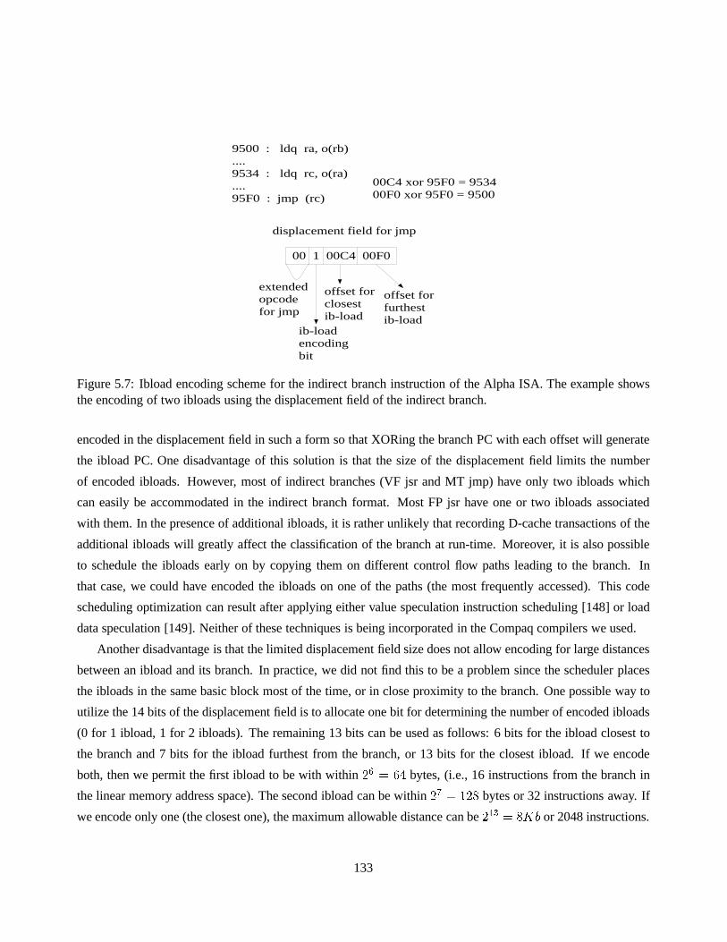
9500 : ldq ra, o(rb)....9534 : ldq rc, o(ra)....95F0 : jmp (rc)

displacement field for jmp

00 1 00C4 00F0

extendedopcode for jmp

ib-loadencodingbit

offset forclosestib-load

offset forfurthestib-load

00C4 xor 95F0 = 953400F0 xor 95F0 = 9500

Figure 5.7: Ibload encoding scheme for the indirect branch instruction of the Alpha ISA. The example showsthe encoding of two ibloads using the displacement field of the indirect branch.

encoded in the displacement field in such a form so that XORingthe branch PC with each offset will generate

the ibload PC. One disadvantage of this solution is that the size of the displacement field limits the number

of encoded ibloads. However, most of indirect branches (VF jsr and MT jmp) have only two ibloads which

can easily be accommodated in the indirect branch format. Most FP jsr have one or two ibloads associated

with them. In the presence of additional ibloads, it is rather unlikely that recording D-cache transactions of the

additional ibloads will greatly affect the classification of the branch at run-time. Moreover, it is also possible

to schedule the ibloads early on by copying them on differentcontrol flow paths leading to the branch. In

that case, we could have encoded the ibloads on one of the paths (the most frequently accessed). This code

scheduling optimization can result after applying either value speculation instruction scheduling [148] or load

data speculation [149]. Neither of these techniques is being incorporated in the Compaq compilers we used.

Another disadvantage is that the limited displacement fieldsize does not allow encoding for large distances

between an ibload and its branch. In practice, we did not find this to be a problem since the scheduler places

the ibloads in the same basic block most of the time, or in close proximity to the branch. One possible way to

utilize the 14 bits of the displacement field is to allocate one bit for determining the number of encoded ibloads

(0 for 1 ibload, 1 for 2 ibloads). The remaining 13 bits can be used as follows: 6 bits for the ibload closest to

the branch and 7 bits for the ibload furthest from the branch,or 13 bits for the closest ibload. If we encode

both, then we permit the first ibload to be with within26 = 64 bytes, (i.e., 16 instructions from the branch in

the linear memory address space). The second ibload can be within 27 = 128 bytes or 32 instructions away. If

we encode only one (the closest one), the maximum allowable distance can be213 = 8Kb or 2048 instructions.

133

Notice that with this range, we can encode ibloads that do notnecessarily lie in the same procedure as the

branch.

An additional solution would be to have dependence checkinghardware identifying the two dependent

instructions (ibload and branch) via their registers when they are decoded. Although this approach works even

in the presence of register remapping it has a number of drawbacks. First, if the dependent instructions are not

decoded in the same cycle, then we must have additional hardware to keep track of which ibloads have not yet

been linked with a branch. Notice that the use of compiler tags relieves the hardware from the burden of finding

ibloads. Second, even if they are decoded in the same cycle, there exist ibloads that are not directly dependent

on the branch. They lie in the dependence chain of the branch,such as the first load shown in the following

assembly code sequence:

ldq rb, o1(ra)ldq rc, o2(rb)jsr (rc)Such code sequences are found in virtual function calls, switch statements implemented with JTBLs and

even in function pointer-based calls. In the latter category, the number of ibloads varies from one to many,

depending on the source code usage of the function pointer. Linking the first ibload with the branch is not

straightforward and necessitates extra hardware support.

Another characteristic of the proposed DTBL implementation is that each entry represents a dependence

between an ibload and its corresponding branch. We could have collapsed the dependencies of two or more

ibloads with the same branch, into one DTBL entry. In a way, wewould capture the entire dependence chain

shown before in a single DTBL entry. That has the advantage ofreducing space since the branch PC does

not have to be copied into multiple DTBL entries. Also, for a fixed storage DTBL space, fewer dependencies

would miss. On the other hand, space would be wasted if only one ibload is detected. If a chain has a variable

length, then information would be lost since each DTBL entrycan accommodate a fixed number of ibloads.

Finally, forming a tag for such a dependence chain is complicated since multiple ibloads have to be detected,

grouped and combined every time. In addition, recording multiple D-cache transactions of the ibloads in the

chain would require complicated hardware support in contrast with the single ibload DTBL entry format.

The DTBL utilizes this dependence information to update themechanism that monitors the D-cache trans-

actions and uniquely links them to indirect branches. TheLoad Miss Table(LMT) is supporting the later task.

The LMT is a tagless table, indexed by the PC of an indirect branch. Each entry contains information about

the load tolerance of that indirect branch. We use a 2-bit up/down saturating counter to measure load tolerance.

Fig. 5.8 shows the counter update protocol.

There are four possible states in the counter. States 2 and 3 indicate low load tolerance and states 0 and 1

134

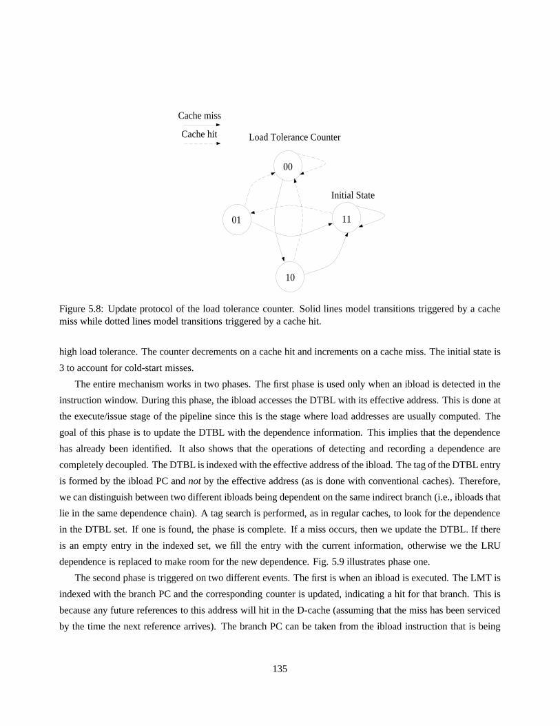
00

01

10

11

Initial State

Load Tolerance Counter

Cache miss

Cache hit

Figure 5.8: Update protocol of the load tolerance counter. Solid lines model transitions triggered by a cachemiss while dotted lines model transitions triggered by a cache hit.

high load tolerance. The counter decrements on a cache hit and increments on a cache miss. The initial state is

3 to account for cold-start misses.

The entire mechanism works in two phases. The first phase is used only when an ibload is detected in the

instruction window. During this phase, the ibload accessesthe DTBL with its effective address. This is done at

the execute/issue stage of the pipeline since this is the stage where load addresses are usually computed. The

goal of this phase is to update the DTBL with the dependence information. This implies that the dependence

has already been identified. It also shows that the operations of detecting and recording a dependence are

completely decoupled. The DTBL is indexed with the effective address of the ibload. The tag of the DTBL entry

is formed by the ibload PC andnot by the effective address (as is done with conventional caches). Therefore,

we can distinguish between two different ibloads being dependent on the same indirect branch (i.e., ibloads that

lie in the same dependence chain). A tag search is performed,as in regular caches, to look for the dependence

in the DTBL set. If one is found, the phase is complete. If a miss occurs, then we update the DTBL. If there

is an empty entry in the indexed set, we fill the entry with the current information, otherwise we the LRU

dependence is replaced to make room for the new dependence. Fig. 5.9 illustrates phase one.

The second phase is triggered on two different events. The first is when an ibload is executed. The LMT is

indexed with the branch PC and the corresponding counter is updated, indicating a hit for that branch. This is

because any future references to this address will hit in theD-cache (assuming that the miss has been serviced

by the time the next reference arrives). The branch PC can be taken from the ibload instruction that is being

135

Tagged (ib) load access

vb Load PC branch PC

DTBL

load effective address

PC branch PCload reg + offset

1

22

To L1 D-cache1

Figure 5.9: Phase 1: when an ibload is executed the dependence between the ibload and the indirect branch isrecorded in the DTBL.

executed (assuming that its entry in the instruction windowhas space for the branch PC). If special hardware is

used to track dependencies on the fly we could have a miss (the hardware was not able to link the ibload with

its branch). In that case, we could use the branch PC stored inthe DTBL if we have a tag match. If we have

a tag mismatch and the branch PC has not yet been defined, we will not update the LMT. Fig. 5.10 shows the

scenario for updating the LMT from an ibload access.

A second phase is also triggered when a load misses in the D-cache and a replacement occurs. The DTBL

is indexed with the address being replaced. Since this address is replaced from the L1 D-cache, it will miss next

time it is referenced. Therefore, the status of all brancheswhose PC’s are found in that set should be updated.

This implies that multiple accesses to the LMT have to be performed. Fig. 5.11 displays the process of updating

the LMT on a D-cache miss for a 2-way set associative DTBL.

The number of LMT accesses is equal to the associativity of the DTBL. One possible solution is to discard

updating all branches and select only one from the DTBL set, probably the one in the MRU dependence.

Another solution is to perform all updates simultaneously (assuming a multi-ported LMT implementation).

The number of ports can be equal to the associativity of the DTBL. Alternatively, we can assume a smaller

number of ports and perform the updates in subsequent cycles. Requests for LMT updates will then need to be

kept in a hardware queue, where each entry will include the branch PC and the cache miss transaction status.

This solution has the advantage of being able to merge updates from the same branch. A final option is to keep

136

load access

vb Load PC branch PC

DTBL

LMT

counter

load effective address

PC branch PCload reg + offset

1

1

To L1 D-cache

DTBL tag match

valid branch PCin load (if load is tagged)

1

3

3

4

2

Figure 5.10: Phase 2: when an ibload is executed we update theDTBL in case its dependence has not alreadybeen recorded. The LMT is updated independently of the DTBL.

the LMT single ported and fill a hardware queue with these requests. One request is posted to the LMT on

each cycle. We assumed the multi-ported implementation in our simulations, mainly for two reasons. One is

that LMT updates do not lie on the critical path of any of the machine’s operations. The other reason is that

we wanted to investigate the potential of our method withoutbeing severely limited by hardware or timing

restrictions.

Notice that LMT updates can be initiated either after a first phase (ibload has caused another line to be

replaced) or independently (a non ibload has triggered a cache miss, and a line is being displaced). Also,

indexing the DTBL is a key component for our mechanism. The DTBL index is formed by applying the exact

same bit selection as in the L1 D-cache. In other words, the same number of bits used for selection within

the cache line is discarded. This does not necessarily mean that the DTBL has a line size equal to that of

the L1 D-cache. The other essential property is for the DTBL to have the same number of sets as the L1 D-

cache. Notice that this does not imply any restrictions on the degree of associativity, which can be different

than the associativity of the L1 D-cache. The philosophy behind this approach is the following: we want the

dependencies inside every DTBL set to correspond to the loads whose addresses are accessing the same set

137

vb Load PC1 branch PC1

LMT

counter

displaced data address1

From L1 D-cache

DTBL (2-way set associative)

vb Load PC2 branch PC2

counter

2

2

DTBL set

load access

Figure 5.11: Phase 2: On a D-cache transaction we update the LMT. The DTBL is accessed with the addressbeing replaced from the D-cache. All branches found in the DTBL set may update the LMT.

in the L1 D-cache. That way, whenever a cache line is replacedin the L1 D-cache, its address can be used to

identify the dependencies (and thus the indirect branches)whose associated ibloads will miss in the cache. This

mapping is guaranteed only when, for a given load address, the same set is selected in both the L1 D-cache and

the DTBL.

This implementation suffers from certain inefficiencies. First, not all branches are updated on D-cache

misses and cache line replacements. Only those branches recorded in the dependencies currently residing in

the DTBL set will be updated. Any branches whose dependencies have been displaced from the DTBL will

not be updated. A fully associative DTBL implementation would provide us with the most accurate results,

although some dependencies would be displaced because of the DTBL’s finite size. Second, the LMT has a

finite size and its mapping is not conflict free. If two branches map to the same LMT entry, the counter will

be erroneously updated and will not accurately measure the branch latency tolerance. In addition, all ibloads

associated with a branch are updating the same LMT counter. Hence, we can not measure load tolerance based

on different ibload instances. For example, if an ibload visits memory locations at addresses100; 200 and300,

the LMT counter will be updated with these 3 cache transactions. After the branch is updated for the last time,

the LMT counter will reflect the tolerance of the branch with respect to those 3 load addresses. If the next time

the branch is fetched, its associated ibload accesses memory location400, the LMT counter will most probably

indicate that the branch tolerance is low, while the ibload may miss in the D-cache. In other words, indirect

138

branch tolerance is specified by merging cache transactionsfrom all addresses visited by its ibloads.

Coupling the LMT with the DTBL would partially solve this problem since the DTBL is indexed by the

load effective address. But it would not merge the data from different ibloads since each counter captures the

tolerance of the branch with respect to the load whose PC is inthe DTBL entry. Most importantly, the LMT

counter contents would be lost if the dependence had to be displaced from DTBL. Coupling the LMT with the

indirect branch predictor entries would allow for a more accurate comparison between the LMT contents of

the current branch and the branch residing in the table entry, during update. This is because the LMT counters

would always be updated. The main problem with this solutionis that path-based predictors allocate multiple

entries for a single indirect branch. Therefore, it is impossible to find all of these entries every time the LMT

must be updated. In addition, the increase in traffic to the indirect branch predictor is prohibitive.

The LMT information can be utilized in many ways. We can access the LMT with the PC of an indirect

branch at the fetch stage of the pipeline, and use the LMT counter contents to improve predictability. For

the reasons mentioned above, we decided to utilize LMT information to enhance the update policy of indirect

branch predictors: If there is a tag mismatch in the indirectbranch predictor and an entry must be displaced

then we check the LMT counters of both branches. The LMT counter associated with the branch updating the

predictor is taken directly from the LMT. The LMT counter associated with the branch currently residing in the

predictor, can be retrieved by an additional LMT access or using a copy in the predictor (which will not be as

recent as the one in the LMT table). Since we may not want to paythe penalty for another LMT table access,

we can have a copy of the LMT counter in the predictor entry. Inany case, the branch with the largest LMT

counter is allocated in the predictor. In the case of a tie, wefavor the branch updating the predictor.

If the predictor has a local copy of the LMT counter and the newbranch replaces the old one, the local

copy can be updated. If the old branch remains in the predictor (no replacement occurs), we can optionally

update the local copy of the LMT counter by accessing the LMT.Notice that our approach works with all

conventional replacement policies (e.g., LRU). The LMT counter associated with the LRU entry is compared

to the LMT counter of the new branch. Alternatively, every time a new branch accesses a set, we could retrieve

the LMT counters of all branches in the set (including the counter of the new branch), compare them and

exclude the branch with the lowest overall value. The major disadvantage of this approach is that the number

of LMT accesses for every predictor update is equal to the associativity of the predictor table. Even for 4-

way set associative tables, the cost of building the LMT can be prohibitive. Another problem that arises only

with the PPM predictor is that the number of update decisionsthat have to be made is equal to the number of

components. The number of times the LMT table has to be consulted is equal to the number of tag mismatches

in the Markov components of the PPM predictor. That increases the necessary number of ports of the LMT

table and its design may become too costly. A solution is to allow only one or two Markov components (from

139

those detecting a tag mismatch) to retrieve LMT counter values. These components could be the higher order

ones since they usually make most of the predictions.

5.5 Temporal Reuse of Indirect Branches

Being able to accurately anticipate the occurrence of a branch can be used in refining the replacement policy

for a branch predictor. Most predictors use set-associative, tagged tables to store previous targets. A conflict

occurs if the number of distinct branches, that is mapped to the same set is greater than the degree of associa-

tivity of the table. This conflict may lead to mispredictionsbased on the interleaving patterns of the branch

dynamic occurrences during the execution of the program. One way to try to minimize these mispredictions

is by predicting whether the branch to be replaced is going tobe executed in the near future. Using a similar

philosophy, we can check if the branch that causes a replacement is going to be executed in the near future.

If we have available accurate indicators that provide us with this information, we can make a more informed

decision on which branch should finally occupy the entry in the set.

The idea is motivated by the fact that the indirect branches that are hardest to predict are those lying inside

loops 4. We have shown in chapter 4 examples in the source code where virtual function or pointer-based

function calls and switch statements are found inside tightloops or recursive functions. It is not uncommon

to traverse dynamically allocated data structures (e.g., linked lists, trees) and make a virtual function call on

every node which corresponds to an object. Depending on the type of the object, the call may visit different

functions, leading to an unpredictable behavior. Similarly, we may scan strings using a loop that contains a

switch statement. The switch statement executes a case based on the character currently being parsed, and thus

its target can change frequently. If we can identify these branches and increase the lifetime of their associated

targets in the predictor, we might be able to improve their predictability.

To capture branch temporal locality, we propose a shift register, called theTemporal Locality Register

(TLR) 5. A TLR can record the addresses (PCs) of a certain number of past committed branches. Since we

are interested in indirect branch locality, we consider a TLR that considers only indirect branches. Indirect

branches of the ret type are excluded. We can also safely exclude all direct branches because an indirect branch

can be displaced only by another indirect branch in an indirect branch predictor. If conditional branches share

the same predictor table with indirect branches (as is usually the case with modern microprocessors), we would

need to record both types of branches in the same or differentregisters.

Our algorithm for exploring the potential of temporal locality of indirect branches is the following: As an

application runs, we count the number of dynamic branches inside a window, the size of which is defined by4Notice that we do not refer to loop branches which are usuallyconditional branches.5An alternative name would beTemporal Reuse Register(TRR).

140

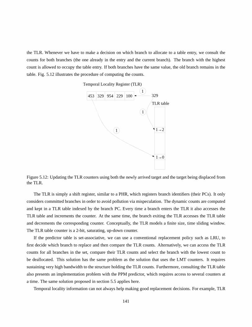
the TLR. Whenever we have to make a decision on which branch toallocate to a table entry, we consult the

counts for both branches (the one already in the entry and thecurrent branch). The branch with the highest

count is allowed to occupy the table entry. If both branches have the same value, the old branch remains in the

table. Fig. 5.12 illustrates the procedure of computing thecounts.

Temporal Locality Register (TLR)

453 329 954 229 100 329

1→2

1

1

1

1→0

TLR table

Figure 5.12: Updating the TLR counters using both the newly arrived target and the target being displaced fromthe TLR.

The TLR is simply a shift register, similar to a PHR, which registers branch identifiers (their PCs). It only

considers committed branches in order to avoid pollution via mispeculation. The dynamic counts are computed

and kept in a TLR table indexed by the branch PC. Every time a branch enters the TLR it also accesses the

TLR table and increments the counter. At the same time, the branch exiting the TLR accesses the TLR table

and decrements the corresponding counter. Conceptually, the TLR models a finite size, time sliding window.

The TLR table counter is a 2-bit, saturating, up-down counter.

If the predictor table is set-associative, we can use a conventional replacement policy such as LRU, to

first decide which branch to replace and then compare the TLR counts. Alternatively, we can access the TLR

counts for all branches in the set, compare their TLR counts and select the branch with the lowest count to

be deallocated. This solution has the same problem as the solution that uses the LMT counters. It requires

sustaining very high bandwidth to the structure holding theTLR counts. Furthermore, consulting the TLR table

also presents an implementation problem with the PPM predictor, which requires access to several counters at

a time. The same solution proposed in section 5.5 applies here.

Temporal locality information can not always help making good replacement decisions. For example, TLR

141

values can not distinguish between the initial and final instance of a branch being executed in a loop. Upon

the first occurrence of the branch, its TLR counter value is 0,showing no temporal reuse and it may not be

allocated in the predictor. Upon the last occurrence of the branch, its TLR counter value will be 3, showing

high temporal reuse. It will take two successive executionsfor a new branch to replace the old one based on

their TLR counters. Similarly, a LMT replacement policy maynot be optimal. If a branch is executed in a tight

loop many times, it is highly likely that its LMT counter willbe 0 (most of the ibloads will hit in the D-cache).

If the branch collides with a branch having a high LMT countervalue, it will be replaced from the predictor

table due to its high load tolerance. This action will displace most of the branch’s targets while the loop is

executed, resulting in a higher number of mispredictions. In order to fix both of the above problems we decided

to combine both approaches in the following manners. If bothbranches show no signs of temporal reuse (TLR

counts are 0), we replace the old branch only if it has a higheror equal load tolerance (a lower or equal LMT

counter value). If the new branch exhibits some temporal reuse, then we replace the old branch, only if its TLR

counter has a higher value than that of the old branch.

5.6 Experimental Results

The results related to indirect branch prediction are obtained using execution-driven simulation with Sim-

pleScalar v3.0 Alpha AXP [61]. The benchmark suite consistsonly of perl, gcc, ixx, edg, troff and eqn. In

order to evaluate the performance of the PPM predictor, we simulate a variety of indirect branch predictors.

Each predictor uses a total of 2K entries and tagged tables tostore branch targets. The list of predictors fol-

lows:� BTB: a 2K entry BTB,� BTB2b: a 2K entry BTB, with 2-bit up/down saturating counter per entry,� GAp: 2 1K entry PHTs, a 10-bit PB path history register recordingthe 2 lower-order bits from each target

(path length = 5) using a gshare indexing scheme, and a 2-bit up/down saturating counter per PHT entry,� Dpath: a Dual-Path hybrid predictor consisting of two GAp predictors and an 512-entry table of 2-bit

up/down selection counters. Each GAp predictor is formed by: a 512 entry 2-way (LRU) PHT, a 24-

bit PHR, a 2-bit up/down saturating counter per PHT entry forreplacement, and a reverse interleaving

indexing scheme. One component predictor has a path length of 2 and the other has a path length of 4.

All recorded bits are lower-order,

142

� Cascade: a Cascade hybrid predictor formed by an identicalDpathpredictor and a Leaky Filter (LF) of

128 entries,� PPM-hyb: a PPM predictor of order 10, 2 100-bit PHRs (PIB and PB path history type, 10 targets, 10

low-order bits each), 10 Markov predictors with total 2K entries, an SFSXS indexing scheme, and a 1K

selection counter table with 2-bit saturating counters perentry.

The predictors are assumed to assist the instruction fetch unit of a dynamically scheduled, out-of-order

CPU, by predicting the target of an indirect branch. All predictors are speculatively updated at the instruction

decode stage of the pipeline. In order to examine the merit ofindirect branch prediction, we also simulate a

base machine with no explicit indirect branch predictor. This configuration is labeled asDft in all tables and

plots. The base machine predicts the targets of all branches, including both indirect and conditional branches,

using a BTB structure. We assume that the BTB is decoupled from the component that predicts the outcome

of conditional branches. The remaining machine configurations use the same BTB for conditional and direct

unconditional branches, but a different IB predictor for indirect branches. Return instructions are predicted

with a fully check-pointed RAS in all configurations [128].

In order to have a fair comparison in terms of hardware cost, the total number of predictor table entries is

the same for both the base machine and the machines employingIB predictors. If the base machine has a BTB

with n entries, a machine using an IB predictor will allocaten2 entries to the IB predictor andn2 to the BTB

holding the targets of the remaining branches.

An additional experiment we perform is to check the effectiveness of indirect branch prediction with an

aggressive instruction fetch unit. Currently, the instruction fetch unit fetches only one cache line from the I-

cache in a single cycle. It discontinues fetching either when the end of the line has been reached or when a

branch is predicted taken. It continues fetching within a single cache line as long as the branch is predicted

non-taken. Hence, the front end can supply up to 8 instructions (L1 I-cache line size is equal to 32 bytes) per

cycle to the decode and dispatch stages. The current trend inprocessor design is towards more aggressive front

ends which attempt to keep the execution units utilized. Thegoal is to reveal a larger window of instructions

and create opportunities for exploiting a larger degree of ILP. At the same time, fetching has to be precise

to minimize mispeculation penalty, which increases as the degree of pipelining gets higher. Therefore, we

simulate a more aggressive fetch unit, where up to 2 cache lines can be brought from the L1 I-cache in a

single cycle. This can be achieved through multi-porting orinterleaving [150, 151]. Interleaving is easier to

implement, requires less area and allows the I-cache banks to operate at high speeds but suffers from bank

collisions. Multi-porting slows down the access time of thecache module, occupies more area, but always

allows two transfers to different cache lines on the same cycle. We decided to model the 2nd case since it does

143

not suffer from bank collisions. We pipelined though the L1 I-cache access in 2 stages to account for the slower

access time.

We exploit the higher I-cache bandwidth by using a two-blockahead branch predictor, similar in spirit to

the one described in [152]. The scheme predicts at most two branches in a single cycle. A predecode unit

provides information about the type and position of all branches found in the cache lines being fetched. All

predictor components are assumed to be dual-ported (BTB, components of hybrid predictor, meta predictor),

enabling two predictions in a single cycle. Every BTB entry (of the unified BTB) is equipped with a bit to

signify whether the branch is the last one in the cache line. Whenever the bit is set, and the conditional branch

is predicted to be non-taken, the next sequential cache lineis simultaneously fetched instead of requesting the

next instruction block which partially lies in the current cache line. This is an optimization suggested in [152]

in order to improve the fetch unit throughput and acts similarly to the oversize bit proposed in [153]. We also

simulate a fully check-pointed dual-ported RAS.

The two-block ahead predictor also predicts indirect branches. Although the dynamic frequency of MT

indirect branches is low, the probability that two such branches are detected in two simultaneously fetched

cache lines from the I-cache is not negligible. In [31], Driesen measured the average execution distance of

indirect branches. He found that 20% of the indirect branches were executed within 1-15 instructions of each

other. Since our cache lines are 8 instructions long, and twocache lines are fetched in a cycle, the probability

of having two indirect branches in two cache lines is not minimal. Therefore, we model a dual-ported BTB

design to permit two indirect branches to be predicted in a single cycle. Hybrid predictors (dpath, cascade,

ppm) require dual-porting their additional components (meta predictor for dpath and ppm, filter for cascade)

in order to sustain the required bandwidth. Since designingmultiple-block indirect branch predictors is out of

the scope of this thesis, we will not elaborate on their design details further. This experiment is performed to

quantify the role of indirect branch prediction in machineswith aggressive fetch policies.

Fig. 5.13 shows a performance comparison for the indirect branch predictors. We plot the relative cycle

count change between the base processor and a processor thatemploys an IB predictor. Data are displayed for

both multiple and single block prediction. Multiple block prediction statistics are labeledaf (aggressive fetch).

A bar with a positive percentage indicates a performance improvement.

Based on the results of Fig. 5.13, indirect branch prediction improves overall performance under certain

conditions. One factor that determines the net effect is therelationship between the conditional branch working

set and the size of the BTB. Decreasing the number of the BTB entries by 50%, to accommodate indirect branch

prediction hardware resources, increases aliasing in the BTB. On the other hand, since traffic assigned to the

same BTB drops (indirect branches are predicted via a separate IB predictor), less aliasing occurs. Obviously,

these two phenomena have competing effects on performance.The amount of aliasing for a specific input

144

0 2 4 6 8 10

BTB

BTB2b

GAg

Dpath

Cascade

PPM

afBTB

afBTB2b

afGAg

afDpath

afCascade

afPPM

Perl: Cycle reduction with IB predictors

Percentage (%)−0.5 0 0.5 1 1.5 2 2.5 3 3.5

BTB

BTB2b

GAg

Dpath

Cascade

PPM

afBTB

afBTB2b

afGAg

afDpath

afCascade

afPPM

Gcc: Cycle reduction with IB predictors

Percentage (%)

−1.5 −1 −0.5 0

BTB

BTB2b

GAg

Dpath

Cascade

PPM

afBTB

afBTB2b

afGAg

afDpath

afCascade

afPPM

Edg: Cycle reduction with IB predictors

Percentage (%)−0.5 0 0.5 1 1.5 2

BTB

BTB2b

GAg

Dpath

Cascade

PPM

afBTB

afBTB2b

afGAg

afDpath

afCascade

afPPM

Troff: Cycle reduction with IB predictors

Percentage (%)

−0.2 0 0.2 0.4 0.6 0.8 1 1.2

BTB

BTB2b

GAg

Dpath

Cascade

PPM

afBTB

afBTB2b

afGAg

afDpath

afCascade

afPPM

Eqn: Cycle reduction with IB predictors

Percentage (%)−1.5 −1 −0.5 0 0.5 1 1.5 2

BTB

BTB2b

GAg

Dpath

Cascade

PPM

afBTB

afBTB2b

afGAg

afDpath

afCascade

afPPM

Ixx: Cycle reduction with IB predictors

Percentage (%)

Figure 5.13: Cycle count reduction/increase when explicitly using IB predictors for predicting indirect branchesother than returns. All results are generated with execution-driven simulation and include speculative traffic.

145

depends on two factors: the mapping employed by the predictor and the branches executed at run-time. The

mapping can be static if the PC of the branch is solely used foraccessing the BTB. Often, past history is used

in conjunction with the branch PC to generate an index. In that case, the mapping is dynamic since the contents

of the history register may be different every time the branch has to be predicted. A conflict miss in the BTB

accompanied with a correct prediction direction generatesa misfetch, which in turn causes the fetch unit to stall.

If the penalty imposed by the extra misfetches offsets the savings from correctly predicting indirect branches

and reduced aliasing in the BTB, then we observe performancedegradation (see edg experiments in Fig. 5.13).

In all other cases, indirect branch prediction is beneficial, reducing the total number of cycles by 0.1% to 10%.

In order to further analyze the effects of indirect branch prediction, we plot the dynamic frequency of

conditional and indirect branches within the simulated time interval for edg and perl. For each benchmark,

we generate four plots for 3 different scenarios. The first includes the base processor configuration while the

other two utilize a processor with the PPM predictor and either a conservative or an aggressive fetch unit.

The plots present the dynamic frequency of conditional and indirect branches and the number of mispredicted

conditional and indirect branches. Each data point is collected within a snapshot that spans 500 clock cycles.

The plots illustrate changes in branch frequency and prediction ratio for the duration of the simulation interval.

A complete set of plots for edg and perl is listed in Appendix C. Fig. 5.14 shows the misprediction ratios for

edg. The left set of plots shows the activity when no indirectbranch predictor is present, while the right plot

shows what happens when the PPM predictor is employed.

Figure 5.14: Conditional and Indirect branch misprediction ratio over time for the edg benchmark. The ratiosare for the base machine (left side) and a machine using a PPM predictor (right side).

146

The misprediction ratios for the conditional branches of edg is higher when half of the BTB space is allo-

cated for the PPM predictor. This increase is more severe at the beginning of the execution since more branches

are competing for the BTB resources (see dynamic counts of conditional branches for edg in Appendix C). Near

the end of the simulation interval, the number of conditional branch mispredictions significantly drops (since

less conditional branches are executed). Fig. 5.15 shows the misprediction ratios for perl. The misprediction

ratio of conditional branches is not adversely affected by the reduced BTB space. On the other hand, indirect

branch mispredictions are eliminated after the predictor is warmed up, and significant performance gains are

observed. Fig. 5.16 provides with the evolution of branch dynamic counts over time for edg and perl. As we

can observe, edg executes a much larger number of conditional branches over time than perl.

When comparing the results between the conservative and theaggressive fetch unit, performance gains do

not always scale with the fetch model. Troff, gcc, perl and eqn display a noticeable increase in performance,

but this is not the case with ixx and edg. Ixx and edg seem to achieve similar gains. IB prediction will

be beneficial as the fetch unit becomes aggressive because itallows for higher utilization of the available I-

cache bandwidth. The amount of this benefit also depends on conditional branch predictor behavior. The

more conditional branches are mispredicted, the greater the benefit obtained from correctly predicting indirect

branches. Since multiple-block ahead prediction applies more pressure on the conditional branch predictor,

the misprediction ratios tends to slightly increase. For example, the total number of mispredictions in the

conditional branch predictor rises by 8.0%, 0.6%, 3.2%, 11.7%, 19.0% and 7.0% for edg, ixx, perl, gcc, troff

and eqn respectively when multiple block prediction is used(all statistics correspond to a machine with no IB

predictor). On the other hand, indirect branch predictor performance appears to improve with multiple block

prediction (with the exception of PPM). For troff, gcc, perland eqn, this leads to better overall performance,

while it maintains performance improvement for ixx and edg.

The problem with the lower misprediction ratio of the PPM predictor (with multiple block prediction) lies

with its mapping function. When two indirect branches need to be predicted in a single cycle, the selected PHR

accesses all components. If a PHR with identical contents isused for both branches, the same entry will be

accessed in all components because the PC of the branch does not currently participate in the index generation.

As a consequence, a larger number of branches alias in the components and the number of mispredictions may

increase up to the point where performance deteriorates (ixx). This situation does not arise in single block

prediction because speculative update in the decode stage inserts an additional target in the PHR before the

indices for the next indirect branch are created.

The PPM predictor outperforms all other configurations mainly due to its lower misprediction ratios which

are plotted in Fig. 5.17. We only list data for the non-aggressive fetch model since our goal is not to elaborate

147

Figure 5.15: Conditional and Indirect branch misprediction ratio over time for the perl benchmark. The ratiosare for the base machine (left side) and a machine using a PPM predictor (right side).

Figure 5.16: Conditional and indirect branch dynamic counts over time for perl (left side) and edg (right side).All results are generated on a base machine (no IB predictor).

148

on good design choices in the field of multiple-block indirect branch prediction. Actually, the higher mispre-

diction ratios achieved by the PPM predictor indicates the need to allow the PC to participate during the index

generation, as described above.

As we can see in Fig. 5.17 the PPM predictor consistently achieves the lowest misprediction ratios, outper-

forming all other predictors. The BTB configurations suffered from the highest misprediction ratios, sometimes

leading to overall performance degradation when compared against the base machine (gcc, troff, eqn). Based

on Fig. 5.13, a lower misprediction ratio has a positive impact on overall performance by reducing the cycle

penalty due to misfetches. An additional gain comes from reducing negative aliasing in the main BTB when

IB prediction is used. For example, in perl, address predictions via the main BTB are heavily influenced by the

indirect branches executed for the selected simulation interval. Wrong address predictions in the unified BTB

increase only by 1.1% (468,572 extra misfetches) when comparing the base configuration to IB prediction with

the PPM algorithm. In edg, the same difference is 9.5% (4,527,411 extra misfetches). The extra overhead is

partially offset by the superior performance of the IB predictor, but overall performance still degrades (0.6%

for the PPM predictor configuration).

If we look more closely at the performance of each individualIB predictor, we observe the following: the

BTB configurations suffer from a large number of mispredictions, since they simply use the previous target to

predict the next one. If the branch does not exhibit high temporal locality, the BTB will not capture behavior

for this branch. In addition, the mapping function allocates only one target per branch in the BTB. If a branch

visits multiple targets, a number of misses will occur because all the targets compete for the same BTB entry.

Two-level path-based predictors such as the GAg almost always perform better than a BTB due to their higher

accuracy (path-guided prediction). The number of tag mismatches (and eventual misfetches) increases with

path-based prediction, since the indexing function allowsdistinct branches to access the same PHT location.

For example in eqn, 721 tag mismatches occur with the GAg, compared to only 174 with the BTB2b predictor.

However, tag mismatches always form the minority of mispredictions (with the exception of PPM) and do not

adversely influence the effectiveness of the predictor. Again, the numbers of total mispredictions for eqn are

60,316 with the BTB2b predictor and 57,953 with the GAg predictor.

The dual path predictor performs better than the GAg whenever the branches are found to exhibit either short

term or long term correlation. In [108], a study on indirect branch correlation highlighted the sensitivity of the

Dpath predictor to the selected path lengths. In our experiments the Dpath predictor provided an advantage

only in certain cases. One reason is that the path lengths cannot be optimal for every application. In addition,

interference in the selector counters (the same selector counter is modified by different branches) and in the

reduced size PHT components (compared to the PHT componentsof a GAg configuration) do not always lead

to significant improvements for the Dpath predictor.

149

0 10 20 30 40 50 60 70 80

BTB

BTB2b

GAg

Dpath

Cascade

PPM

Perl: IB misprediction ratios

Percent (%)0 10 20 30 40 50 60 70

BTB

BTB2b

GAg

Dpath

Cascade

PPM

Gcc: IB misprediction ratios

Percent (%)

0 5 10 15 20 25 30 35

BTB

BTB2b

GAg

Dpath

Cascade

PPM

Edg: IB misprediction ratios

Percent (%)0 5 10 15 20 25

BTB

BTB2b

GAg

Dpath

Cascade

PPM

Troff: IB misprediction ratios

Percent (%)

0 5 10 15 20 25

BTB

BTB2b

GAg

Dpath

Cascade

PPM

Eqn: IB misprediction ratios

Percent (%)0 1 2 3 4 5

BTB

BTB2b

GAg

Dpath

Cascade

PPM

Ixx: IB misprediction ratios

Percent (%)

Figure 5.17: Misprediction ratios of various IB predictors. All results are generated with execution-drivensimulation. All predictors are updated speculatively.

150

The cascade predictor does not provide any significant gainscompared to the dual path predictor. In order

to investigate this relationship, we measured the number oflookups performed to the different components

of the predictor (Table 5.1). We also present (column 6) the number of times the filter was used to make a

prediction, but mispredicted. Notice that since the filter is tagless we can not distinguish between tag and

target mispredictions. As we can see, the filter reduces the traffic to the main component and provides us with

more correct predictions. This is expected, given the percentage of monomorphic branches in our benchmarks.

However, performance does not increase because the workingset of indirect branches for the simulated interval

is not large enough to stress the Dpath predictor. In [145] weran all benchmarks to completion, and we found

that the cascade predictor lowered misprediction ratios because the main component could not accommodate

all branch instances.

Program PredictionsTotal Long path comp Short path comp filter filter mispred.

perl 2,304,171 1,555,623 344,023 404,525 47,551gcc 1,690,742 753,326 622,260 315,156 219,342edg 2,032,334 623,939 975,650 432,745 232,580troff 987,800 379,999 448,794 159,007 36,571eqn 329,762 76,141 171,980 81,641 30,410ixx 1,357,923 495,124 654,267 208,532 40,356

Table 5.1: Breakdown of predictions for a Cascaded predictor. The classification includes the total numberof lookups (column 2), the number of lookups made the long path (column 3) and the short path component(column 4), the number of filter lookups (column 5) and the number of filter mispredictions (column 6).

The PPM predictor performed the best due to its ability to adjust the path correlation type at run-time,

and explore multiple lengths of path correlation. By distributing the same target to multiple components, the

predictor increased the target’s lifetime. Table 5.2 classifies the number of mispredictions into tag and target.

Table 5.2 shows that tag mispredictions form a significant portion. It seems that different targets (and their

associated indirect branches) have different temporal locality. Some branches are frequently executed inside

loops or recursive procedure calls, while some others are either detected infrequently in the instruction stream

or their temporal locality is very poor. This distinction isnot made explicitly in any other predictor. Hybrid

versions such as the Dpath and the Cascade predictors, partition their resources in order to dynamically assign

indirect branches to their best component and do not exploittarget temporal locality. Path-based predictors or

components access a single table, and based on the previous path history, they may store a target in different

table locations. The PPM predictor obeys the same principle. However, the path correlation length is fixed, and

151

Program Tag Targetperl 49 21,366gcc 39,768 208,530edg 76,866 235,075troff 5,547 86,164eqn 9,046 28,040ixx 10,038 12,002

Table 5.2: Number of mispredictions for a PPM predictor. Column 2 lists the number of tag mismatches andcolumn 3 includes the number of target mispredictions.

if it is not optimal (longer or shorter that it should be), thetarget will be replaced in the table before it is visited.

Fig. 5.18 displays the average occupancy for the I-fetch queue and the centralized instruction window of

the processor configurations with and without indirect branch prediction. Statistics are presented for both fetch

models in number of instructions. Again, theaf label determines the fetch model. Results are shown for perl

and gcc, while the plots for the entire benchmark suite can befound in Appendix D.

Results in Fig. 5.18 show that indirect branch prediction does not have a significant impact on the instruction

fetch queue or the instruction window. The only exception iswhen aliasing in the main BTB is not high enough

to offset the effects of IB prediction. Instruction fetch queue occupancy lie in the same levels except for perl

where indirect branches form an obstacle in exploring higher degrees of ILP. Higher occupancy is even more

noticeable when the aggressive I-fetch unit is employed since the high dynamic frequency of indirect branches

and the IB predictor permit a better exploitation of the available I-cache bandwidth. Similar results can be seen

for the instruction window.

An additional factor affected by IB prediction is the numberof instructions fetched from the wrong path. In

a dynamically scheduled, out-of-order processor employing control speculation in the form of branch predic-

tion, instructions are squashed after a branch misprediction is detected. Table 5.3 lists the number of committed

(executed) instructions in column 2 (columns 3-9). The amount of wrong path execution introduced by indirect

branch prediction is consistently reduced for all applications, including edg, where performance is degraded

after applying indirect branch prediction. The number of squashed instructions depends on the number of

mispredictions and the number of instructions fetched after a mispredicted branch until the misprediction is

detected.

In general, indirect branch prediction allows more indirect branches to be predicted correctly. The behavior

in the main BTB is somewhat different. Since less traffic is guided to the BTB, less aliasing occurs. On the

other hand, since its capacity has been halved to keep the cost budget fair, more aliasing occurs. Depending

152

0 5 10 15 20 25

Dft

BTB

BTB2b

GAg

Dpath

Cascade

PPM

afDft

afBTB

afBTB2b

afGAg

afDpath

afCascade

afPPM

Perl: IFQ occupancy with IB predictors

Ifq occupancy (insns)0 2 4 6 8 10 12 14

Dft

BTB

BTB2b

GAg

Dpath

Cascade

PPM

afDft

afBTB

afBTB2b

afGAg

afDpath

afCascade

afPPM

Gcc: IFQ occupancy with IB predictors

Ifq occupancy (insns)

0 10 20 30 40 50

Dft

BTB

BTB2b

GAg

Dpath

Cascade

PPM

afDft

afBTB

afBTB2b

afGAg

afDpath

afCascade

afPPM

Perl: Instruction window occupancy with IB predictors

insns0 5 10 15 20 25 30 35

Dft

BTB

BTB2b

GAg

Dpath

Cascade

PPM

afDft

afBTB

afBTB2b

afGAg

afDpath

afCascade

afPPM

Gcc: Instruction window occupancy with IB predictors

insns

Figure 5.18: Average I-fetch queue and instruction window occupancy in the presence of IB prediction. Resultsare presented for a machine with either a conservative (lower 7 rows) or an aggressive fetch unit (upper 7 rows).

on the strength of each particular phenomenon, we may have anincrease or a decrease in the total number of

mispredictions. In general, whenever performance improved, the total number of mispredictions has fallen,

leading to a smaller amount of mispeculation.

However, in edg, we still observe a small, but consistent, decrease in the number of mispeculated instruc-

tions across all indirect branch predictor configurations.Notice that edg is the only benchmark presenting

performance degradation when indirect branch prediction is employed. After investigating this issue, we found

that 37.1% of indirect branches are mispredicted on the basemachine with a unified BTB, while 17.4% of

the indirect branches are mispredicted with the PPM predictor, in edg. If we translate that into absolute num-

bers, the PPM predictor mispredicted 301,789 times, while the unified BTB mispredicted 643,085 times. This

significantly reduces the number of mispeculated instructions, but still does not explain the small decrease in

153

Program committed executed (in M)insn (M) Base BTB1b BTB2b GAg Dpath Cascade PPM

perl 300 353.5 353.2 351.9 338.5 336.9 336.4 319.6gcc 300 379.2 376.0 373.5 369.2 372.1 371.2 356.9edg 300 337.4 335.5 334.3 333.3 334.0 332.9 329.7troff 145 157.8 157.9 156.7 156.4 156.8 156.5 156.0eqn 70.1 79.6 79.5 79.4 79.4 79.4 79.3 78.9ixx 52.7 59.2 59.0 58.9 59.0 59.1 58.7 58.3

Table 5.3: Number of committed/executed instructions for machines employing IB prediction. The number ofcommitted instructions is presented in column 2 while the number of executed instructions follows in columns3-9.

mispeculated instructions, since the number of conditional branch mispredictions increased in the machine with

indirect branch prediction for edg. The answer probably lies with the wrong paths fetched whenever an indirect

branch is mispredicted. Indirect procedure calls transfercontrol flow to the beginning of procedures. Storing

callee saved registers and stack manipulation instructions usually lie in the procedure prologue. Most condi-

tional branches following the procedure prologue are non-taken most of the time, since they often correspond

to error checking code. Both of the above factors increase the average number of instructions fetched on an

indirect call prediction. Thus, improving indirect branchprediction can reduce the overall speculative instruc-

tion count even in the presence of poorer conditional branchaccuracy. Notice that predicting direct procedure

calls also contributes to speculative traffic. However, direct calls are always taken (no need for outcome pre-

diction) and their target never changes. If the target is recorded in the BTB, the branch will be always correctly

predicted.

We also study the effects of speculation via indirect branchprediction on I-cache performance. Speculative

execution has both positive and negative effects on I-cacheaccess patterns. It triggers useful prefetches, bring-

ing wrong path instructions closer to the processor, but it may also cause pollution by replacing code that needs

to be referenced [104]. Indirect branches tend to access a different cache line most of the time. For example in

edg, 94% of indirect branches transfer control flow to another cache line, while 88.6% of conditional branches

find their target in the same cache line. This result is expected because indirect procedure calls will access a

procedure that most likely starts from a different cache line. Only switch-based jmps may visit a target that lies

in the same cache line. This does not happen very often due to their low target locality. Accessing different

cache lines does not necessarily lead to lower cache performance. Table 5.4 presents the number of L1 I-cache

accesses and misses, expressed in millions of instructions, for all machine configurations.

154

Program L1 I-cache # of accesses/misses (in M)Base BTB1b BTB2b GAg Dpath Cascade PPM

perl 365/3.73 365/3.73 364/3.71 344/3.74 342/3.76 345/3.77 326/3.82gcc 398/8.53 395/8.50 392/8.49 382/8.49 385/8.49 390/8.51 371/8.47edg 430/16.90 358/16.89 356/16.88 351/16.88 351/16.90 355/16.92 347/16.81troff 163/3.13 163/3.12 162/3.11 160/3.10 161/3.11 161/3.12 160/3.09eqn 82/0.61 82/0.61 82/0.61 81/0.61 81/0.61 81/0.61 81/0.61ixx 61/0.80 61/0.80 61/0.80 59/0.80 59/0.80 60/0.83 58/0.79

Table 5.4: L1 I-cache number of accesses and misses for a basemachine (column 2) and machines employingIB prediction (columns 3-8).

Two conclusions can be drawn. First, the absolute number of I-cache misses does not significantly change

when using IB prediction or across different IB predictors.Hence, IB prediction does not seem to hurt I-cache

performance due to pollution. Second, the number of I-cacheaccesses decreases with IB prediction, saving

valuable I-cache bandwidth. The difference in the number ofI-cache accesses and the number of wrong path

instructions is due to the number of instructions that are squashed before being decoded and issued. This

number is quite significant for certain benchmarks, such as edg. The remaining savings in cache bandwidth

follows the decrease in the amount of mispeculation observed in Table 5.3.

In addition to the experiments for the PPM predictor, we alsoconduct simulations to test the effectiveness

of the replacement policies described in sections 5.4 and 5.5. We modified the replacement policies of the

BTB2b, GAg and PPM predictors with the combined TLR/LMT policy presented at the end of section 5.5.

All parameters of the three predictors remain the same except for their table size, which was reduced to 1K

entries. All simulations model a 6-entry TLR, a tagged 4-wayset associative DTBL with 256 sets (since the

L1 D-cache has 256 sets) and a direct mapped, tagless LMT with1024 entries. We compare the misprediction

ratios in Table 5.5.

Results in Table 5.5 are mixed. Perl’s mispredictions are hardly affected, because the vast majority of

mispredictions comes from target conflicts and not from tag mismatches. In other words, most of the time a

misprediction occurs because, although the same branch occupies the entry of the table making the prediction

(tag match), the wrong target is stored (target mismatch). The very small number of activated static indirect

branches is responsible. Notice that our replacement policy currently focuses only on tag mismatches because

we compare the TLR and LMT values between two distinct staticindirect branches. A future design could

expand both schemes to cover run-time instances of the same branch. That would require recording dynamic

instances of branches for the TLR table. The LMT would also necessitate observing dynamic instances of

155

Program Misprediction ratioLRU policy TLR/LMT policy

BTB2b GAg PPM BTB2b GAg PPMperl 75.58 13.76 0.18 75.56 13.76 0.18gcc 57.81 41.52 20.64 57.81 41.62 21.23edg 32.09 28.78 21.56 32.10 29.79 23.19troff 14.93 11.73 9.92 14.93 11.77 10.11eqn 20.12 19.20 14.62 20.12 19.22 14.29ixx 4.33 4.48 3.14 4.33 4.53 3.00

Table 5.5: Misprediction ratios for IB predictors with LRU (columns 2-4) and TLR/LMT replacement policies(columns 5-7). All results are generated using execution-driven simulation.

ibloads in order to link them with their corresponding run-time branch instances.

The same dominant phenomenon of target mismatches surfaceson all BTB2b experiments because BTB2b’s

suffer from very few tag mispredictions and the new replacement policy has no significant effect. Recall that a

BTB2b is indexed by the PC of the branch only. This is not the case with the GAg predictor. Tag mismatches

make up a significant portion of the predictor’s performanceloss, but our policies do not appear to benefit the

predictor. The reason is that by changing the lifetime of branches in the predictor, a number of target mispre-

dictions is eliminated, while a number of tag mispredictions is introduced. The later phenomenon seems to

overcome the positive effects of the LMT/TLR policy, leading to a negative overall result. Eqn and ixx present

a noticeable improvement with PPM, while the remaining simulations show some degradation on the mispre-

diction ratio. PPM appears to benefit from this policy because it naturally increases the lifetime of individual

branch targets by distributing them to multiple locations across its components. Hence, when a branch remains

in one component, it may be replaced in another. Overall performance may increase if the TLR/LMT policy

manages to properly assign branches. The corresponding cycle counts show similar trends. Overall, we believe

that further work is needed in order to adjust the replacement heuristics and better exploit information about

the temporal reuse and load tolerance of branches.

In order to distinguish between the features of the TLR/LMT scheme that contribute the most, we measure

the number of times this new policy does not displace the old branch in the predictor table. This signifies how

much our policy deviates from a true LRU policy that always replaces the old branch (or the one in the LRU

entry). Furthermore, we break down these decisions into twogroups. One group includes all decisions guided

by load tolerance and the other group contains modified decisions activated by temporal frequency. Results are

presented in Table 5.6, where columns 2, 5 and 8 list the totalsum of replacement decisions made for each

156

benchmark. The remaining columns present the number of alternative decisions. No results are shown for perl

due to their insignificant statistical nature. The numbers for PPM are the sum of replacement decisions over all

Markov components.

Program Modified Replacement DecisionsBTB2b GAg PPM

total ldtol tlr total ldtol tlr total ldtol tlrgcc 789902 5 0 568707 2149 26 2610450 253154 55929edg 556015 184 0 516481 23176 18 3614481 813906 88346troff 138801 45 0 109405 616 0 845793 46566 3833eqn 60491 5 0 57719 158 0 395775 41766 10602ixx 51611 5 0 53407 668 17 336312 30118 1730

Table 5.6: Breakdown of replacement decisions for IB predictors using the TLR/LMT replacement policy.Columns 2, 5 and 8 list the total number of replacement decisions. Columns 3, 6 and 9 present the number oftimes the TLR/LMT policy deviates from LRU and replaces a branch using the LMT counters. Columns 4, 7and 10 present the number of times the TLR/LMT policy deviates from LRU and replaces a branch using theTLR counters.

Based on the results of Table 5.6, it is easy to conclude that load tolerance decisions dominate the activity

of our scheme. Furthermore, the number of times our policy deviates from LRU is rather small. Decisions

based on load tolerance are characterized by the fact that both branches do not seem to have temporal reuse

(their TLR counters are both 0). The newly arrived branch hasvery low load tolerance. This is expected, since

a branch that has not been seen in the past (TLR counter equals0) is highly likely to have its ibload(s) miss in

the L1 D-cache when re-referenced. A branch that is already in the predictor generally keeps the data accessed

by its ibloads in the cache. The number of times the ib-load misses is shown in columns labeled asldtol. These

cases represent branches that remained in the predictor buttheir ibloads have already been evicted from the L1

D-cache due to poor temporal locality.

Decisions based on TLR counters relate branches that have some recent temporal reuse. The LRU branch

is replaced unless its TLR counter is larger than, or equal to, that of the new branch. This situation corresponds

to the following scenario: the branch already in the predictor has been executed a number of times, while the

new branch has recently entered the temporal window captured by TLR. If control flow departs from the old

branch and remains within the new branch, the decision made by our policy will benefit the prediction scheme

in the long run. Otherwise, the hysteresis provided by the TLR counters will slow down the responsiveness of

the predictor causing a larger number of tag mispredictions.

157

5.7 Summary

We have presented the PPM predictor as a new model for predicting values. We have evaluated its potential

on the field of indirect branch prediction and showed that howour proposed implementation exploits multiple

length path correlation. We have enhanced the original PPM design with run-time selection of path history type.

We have also introduced the use of temporal reuse and load tolerance information in indirect branch prediction.

Our results showed that PPM prediction is a viable alternative to a set of other branch predictor strategies.

We have also demonstrated that indirect branch prediction can be cost-effective and improve performance

under certain conditions. Two crucial factors determiningthe effectiveness of indirect branch prediction are the

relation between the conditional branch working set size and the main BTB size as well as the corresponding

relation between the indirect branch working set size and the indirect branch predictor size.

158

Chapter 6

Conclusions and Future Work

6.1 Contributions

The main contributions of this thesis are the following: First, we have proposed a new model that accurately

records temporal procedure interaction using the L1 cache organization. We also described a new algorithm

for performing code placement in a memory hierarchy with multiple cache levels. Second, we characterized

the behavior of indirect branches and we introduced two new hardware-based methods for improving their

predictability. Finally, we have verified that the above techniques can be successfully applied to both proce-

dural and Object-Oriented languages, by using a set of C and C++ programs as our application suite. More

specifically, we have made the following contributions:� A systematic way to measure both the temporal interaction ofcode modules and the potential of ex-

ploiting temporal locality in code reordering through the CMG graph. To the best of our knowledge,

only the TRG model [55] uses temporal information for code reordering but works at a coarser level of

granularity.� A set of algorithms that target the minimization of conflict misses in a multi-level cache hierarchy via

procedure and/or intraprocedural basic block reordering.Our approach is the first technique published

that reorders code modules in a multi-level cache hierarchywith caches of arbitrary size, line size and

associativity. It is also the first work combining temporal procedure reordering with intraprocedural basic

block reordering.� A study on indirect branch predictability, entropy, correlation. This work reaches certain conclusions

about the expected behavior of indirect branches supportedby source code examples.

159

� Several hardware-based methods for improving indirect branch prediction. We demonstrate the potential

of techniques such as variable length path correlation, run-time selection of path correlation type and

replacement based on both load tolerance and temporal locality.� A detailed study on the performance potential and necessityof indirect branch prediction for superscalar

machines employing speculative execution.

6.2 Future Research on Code Reordering

There exist many ways that we could improve or extend the workdescribed in code reordering. We should

consider ways to optimize shared code such as dynamically linked libraries (DLLs). Since DLLs are utilized by

different applications, many times under diametrically opposite scenarios, various profile data streams should

be combined in order to uniformly optimize shared code. We could also evaluate the performance of optimized

executables via code reordering, in the presence of multiprogramming or multi-threading. Both techniques may

stress shared resources, such as the cache hierarchy [154].

Examining the potential of combining cache conscious code reordering and instruction prefetching has

shown promising results [84]. More work is needed though to establish the interaction between different

prefetching and code reordering techniques. Refining the basic block reordering algorithm to explicitly take

into account the activity of a sophisticated hardware basedprefetcher, may be beneficial. We can also modify

such algorithms to detect paths using techniques such as intraprocedural [100, 90] and interprocedural path

profiling [155]. On the other hand, when mapping to multiple caches, prefetching between the L1 and L2

can increase the efficiency of an improved (L1,L2) combined mapping. Accesses that hit in the L2 instead of

missing due to code mapping could initiate useful prefetches.

The area of dynamic code placement seems to be an increasingly popular research avenue. As dynamic

compilation systems mature, we expect more and more optimizations to be performed entirely or partially at

run-time. Code reordering has proven that it can improve performance using past behavior of the application’s

most frequently accessed code segments. However, profile-based solutions do not adapt in time when the

application changes behavior. The training scenario can not always exercise every code module in a large

application. Therefore, dynamic techniques may be needed in the future. Their run-time cost though is still too

high. Although procedure placement at run-time is feasible[81, 82], reordering basic blocks is cumbersome

and no implementation has been published so far. Even dynamic procedure reordering has not been investigated

in depth. Since run-time TRG/CMG construction is unreasonable in terms of time overhead, a new temporal

model is necessary to be deployed in a run-time system. Hardware support for code reordering may also be

beneficial. Recently, a fast and efficient scheme has been proposed for detecting conflict misses at run-time

160

[156]. Such information can be communicated to run-time threads to trigger code repositioning.

Looking back to our original CMG model, we can modify the way we update CMG edge weights by

assigning probabilities to the live cache lines. A live cache line lying at the end of the LRU stack has a smaller

probability of causing a conflict miss than the cache line lying at the beginning. We can also define a hybrid

model that stands somewhere between the CMG and the TRG. We could define the temporal window size and

its replacement policy based on the set of activated cache lines as it is done with the CMG instead of using

static procedure sizes as it is done with the TRG. On the otherhand, edge weights could be updated as it is

suggested in the TRG, by simply incrementing the edge weightby 1 every time two procedures are found to

interact inside the temporal window.

Since caches (other than the 1st level) usually handle both instruction and data references, there exists a

significant number of conflicts between the two streams. Mostof the research on data placement has focused on

reorganizing loops and data in a cache-conscious manner to improve the locality and hit ratio of data accesses

[157, 158]. Other techniques have promoted intelligent data structure layout and/or variable allocation [159,

160, 161]. However none of the above schemes integrates instruction and data placement in a unified cache

level or in main memory.

An additional, but equally important, direction is to combine code reordering for virtually accessed L1

caches with physically indexed L2 caches. When physical addresses access an L2 cache, instruction (and data)

mapping in the L2 cache depends on which virtual pages overlap in the cache address space. Compiler-directed

page placement and operating system support for page coloring are two methods that can potentially reduce

the number of conflicts [162, 163]. Hardware support for either solution can even further improve performance

[62, 65].

6.3 Future Research on Indirect Branch Prediction

There are several future avenues of research in the field of indirect branch prediction. First, we could investigate

the synergy between an indirect branch predictor and an engine that prefetches ib-loads, similar to the one

described in [134]. Early execution of ib-loads can assist branch predictability when prefetching the register

value used by the indirect branch to form its target.

An additional approach would be to combine a victim buffer with a DTBL and a TLR register. The victim

buffer could hold data accessed by ib-loads when being replaced from the L1 D-cache. Data would enter the

victim buffer only when the branches in the DTBL entry appearto be temporally reusable. When the next ib-

load executes the victim buffer would be searched, and only if no match is found in the buffer, the L1 D-cache

would be accessed. The benefit of this approach would be, not only the reduction of D-cache misses and their

161

associated cycle penalty, but also the reduction of indirect branch resolution time.

Furthermore, we can improve the replacement policy introduced in Chapter 5 by recording dynamic instead

of static dependencies between ib-loads and indirect branches. The DTBL would store targets of indirect

branches therefore linking the target of an ib-load with thebranch target. Uniquely identifying a dynamic

load requires combining its PC with its target address. The DTBL already stores the load PC in its tag field.

Similarly we could store both the branch PC and its target to uniquely identify the branch dynamic instance.

The LMT table would be indexed by branch targets and would reflect the load tolerance of a branch instance.

Although the amount of aliasing in the LMT would be higher (there are more indirect branch targets than

indirect branches), the information would be more accurate. An additional feature could be to add the branch

PC to each LMT entry as a tag, in order to identify aliasing between different branch instances.

The TLR structures could also be modified to record the temporal reuse of indirect branch targets. The

TLR would essentially become a PHR recording a subset of PIB history since no return instructions would

need to feed their targets to the TLR. The TLR table would be indexed by branch targets. An alternative

approach would be to record branch or branch target entropy:how many times two branches are interleaved in

the dynamic instruction stream or how frequently a branch target changes between two successive executions.

One possible implementation would be a two-dimensional bitmatrix indexed by branch PCs or branch targets.

Branch or target entropy could be useful with small predictor sizes where aliasing is the dominant effect. It

could also assist the distribution of branches to the components of a hybrid predictor. For example, if two

branches frequently follow each other and map to the same table entry at run-time we could allocate their

targets to different components of the predictor.

Load tolerance and temporal reuse information may also be exploited in alternative ways. With the cur-

rent trend in microprocessor design, high clock frequencies prohibit having complicated, single-cycle access

predictor structures. Pipelining and hierarchical prediction are two techniques currently in use to overcome

this problem. Complex predictors, whose critical path doesnot fit in a single pipeline stage, are themselves

pipelined. A hierarchy of predictor schemes may also be implemented: a next set predictor in the I-cache at the

1st level [164], a 2-bit BTB in the 2nd level, a hybrid/two-level predictor at the 3rd level, etc. This hierarchy

may act as a filter, since not all branches require complex predictor mechanisms to be predicted correctly. Load

tolerance information can serve such a filtering role by allowing temporal and low tolerant branches to use the

most accurate component or level of prediction only. On the other hand, non-temporal branches with high load

tolerance may be serviced from a lower level of the prediction hierarchy. Non-temporal branches with low

tolerance could avoid allocating an entry in the most accurate predictor. Temporal branches with high tolerance

are those that should flow through the entire hierarchy to obtain the best possible decision.

We can also attempt to design indirect branch predictors with structures similar to the ones described for

162

value predictors [123, 143, 165]. Likewise, we can examine the potential of using the PPM algorithm in value

prediction. Hybrid schemes can also be devised in order to filter run-time constant values, and values that

follow stride patterns, from the PPM predictor.

A series of compiler techniques can modify the static and dynamic population of indirect branches, as well

as their impact on performance. Some of these include polymorphic call resolution, predication, conditional

branch elimination, replacement of series of conditional branches with indirect jumps, dynamic linking with

indirect call transformation, etc. Examining their cooperation with hardware-based indirect branch prediction,

or comparing their effectiveness against the later, shouldbe another interesting research direction.

163

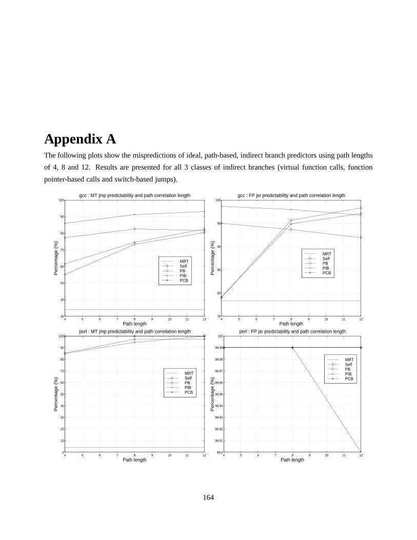
Appendix AThe following plots show the mispredictions of ideal, path-based, indirect branch predictors using path lengths

of 4, 8 and 12. Results are presented for all 3 classes of indirect branches (virtual function calls, function

pointer-based calls and switch-based jumps).

4 5 6 7 8 9 10 11 1230

40

50

60

70

80

90

100gcc : MT jmp predictability and path correlation length

Pe

rce

nta

ge

(%

)

Path length

MRTSelfPBPIBPCB

4 5 6 7 8 9 10 11 1275

80

85

90

95

100gcc : FP jsr predictability and path correlation length

Pe

rce

nta

ge

(%

)

Path length

MRTSelfPBPIBPCB

4 5 6 7 8 9 10 11 120

10

20

30

40

50

60

70

80

90

100perl : MT jmp predictability and path correlation length

Pe

rce

nta

ge

(%

)

Path length

MRTSelfPBPIBPCB

4 5 6 7 8 9 10 11 1299.9

99.91

99.92

99.93

99.94

99.95

99.96

99.97

99.98

99.99

100perl : FP jsr predictability and path correlation length

Pe

rce

nta

ge

(%

)

Path length

MRTSelfPBPIBPCB

164

4 5 6 7 8 9 10 11 1240

45

50

55

60

65

70

75

80

85edg : MT jmp predictability and path correlation length

Pe

rce

nta

ge

(%

)

Path length

MRTSelfPBPIBPCB

4 5 6 7 8 9 10 11 1298.4

98.6

98.8

99

99.2

99.4

99.6

99.8

100edg : FP jsr predictability and path correlation length

Pe

rce

nta

ge

(%

)

Path length

MRTSelfPBPIBPCB

4 5 6 7 8 9 10 11 1245

50

55

60

65

70

75

80

85

90

95gs : MT jmp predictability and path correlation length

Pe

rce

nta

ge

(%

)

Path length

MRTSelfPBPIBPCB

4 5 6 7 8 9 10 11 1278

80

82

84

86

88

90

92

94

96

98gs : FP jsr predictability and path correlation length

Pe

rce

nta

ge

(%

)

Path length

MRTSelfPBPIBPCB

165

4 5 6 7 8 9 10 11 1230

40

50

60

70

80

90

100troff : MT jmp predictability and path correlation length

Pe

rce

nta

ge

(%

)

Path length

MRTSelfPBPIBPCB

4 5 6 7 8 9 10 11 1298.2

98.3

98.4

98.5

98.6

98.7

98.8

98.9

99

99.1

99.2troff : FP jsr predictability and path correlation length

Pe

rce

nta

ge

(%

)

Path length

MRTSelfPBPIBPCB

4 5 6 7 8 9 10 11 1279

80

81

82

83

84

85

86

87

88troff : VF jsr predictability and path correlation length

Pe

rce

nta

ge

(%

)

Path length

MRTSelfPBPIBPCB

4 5 6 7 8 9 10 11 1255

60

65

70

75

80

85

90

95eqn : MT jmp predictability and path correlation length

Pe

rce

nta

ge

(%

)

Path length

MRTSelfPBPIBPCB

4 5 6 7 8 9 10 11 1298.8

99

99.2

99.4

99.6

99.8

100

100.2eqn : FP jsr predictability and path correlation length

Pe

rce

nta

ge

(%

)

Path length

MRTSelfPBPIBPCB

4 5 6 7 8 9 10 11 1266

68

70

72

74

76

78

80

82eqn : VF jsr predictability and path correlation length

Pe

rce

nta

ge

(%

)

Path length

MRTSelfPBPIBPCB

166

4 5 6 7 8 9 10 11 1245

50

55

60

65

70

75

80

85

90bore : MT jmp predictability and path correlation length

Pe

rce

nta

ge

(%

)

Path length

MRTSelfPBPIBPCB

4 5 6 7 8 9 10 11 1289

90

91

92

93

94

95

96

97

98

99bore : FP jsr predictability and path correlation length

Pe

rce

nta

ge

(%

)

Path length

MRTSelfPBPIBPCB

4 5 6 7 8 9 10 11 1289

90

91

92

93

94

95bore : VF jsr predictability and path correlation length

Pe

rce

nta

ge

(%

)

Path length

MRTSelfPBPIBPCB

4 5 6 7 8 9 10 11 1245

50

55

60

65

70

75

80porky : MT jmp predictability and path correlation length

Pe

rce

nta

ge

(%

)

Path length

MRTSelfPBPIBPCB

4 5 6 7 8 9 10 11 1284

86

88

90

92

94

96

98porky : FP jsr predictability and path correlation length

Pe

rce

nta

ge

(%

)

Path length

MRTSelfPBPIBPCB

4 5 6 7 8 9 10 11 1296.2

96.4

96.6

96.8

97

97.2

97.4

97.6

97.8

98

98.2porky : VF jsr predictability and path correlation length

Pe

rce

nta

ge

(%

)

Path length

MRTSelfPBPIBPCB

167

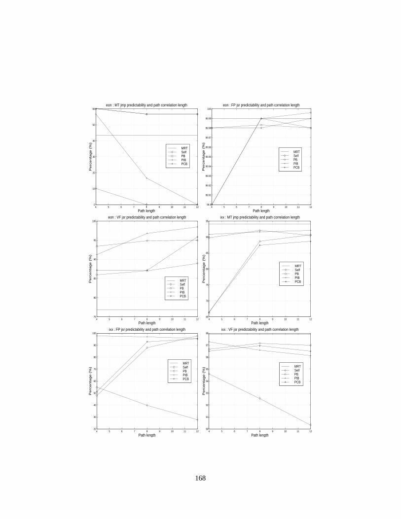
4 5 6 7 8 9 10 11 120

10

20

30

40

50

60eon : MT jmp predictability and path correlation length

Pe

rce

nta

ge

(%

)

Path length

MRTSelfPBPIBPCB

4 5 6 7 8 9 10 11 1299.9

99.91

99.92

99.93

99.94

99.95

99.96

99.97

99.98

99.99

100eon : FP jsr predictability and path correlation length

Pe

rce

nta

ge

(%

)

Path length

MRTSelfPBPIBPCB

4 5 6 7 8 9 10 11 1275

80

85

90

95

100eon : VF jsr predictability and path correlation length

Pe

rce

nta

ge

(%

)

Path length

MRTSelfPBPIBPCB

4 5 6 7 8 9 10 11 1265

70

75

80

85

90

95ixx : MT jmp predictability and path correlation length

Pe

rce

nta

ge

(%

)

Path length

MRTSelfPBPIBPCB

4 5 6 7 8 9 10 11 1220

30

40

50

60

70

80

90

100ixx : FP jsr predictability and path correlation length

Pe

rce

nta

ge

(%

)

Path length

MRTSelfPBPIBPCB

4 5 6 7 8 9 10 11 1290

91

92

93

94

95

96

97

98ixx : VF jsr predictability and path correlation length

Pe

rce

nta

ge

(%

)

Path length

MRTSelfPBPIBPCB

168

4 5 6 7 8 9 10 11 1260

65

70

75

80

85

90

95

100lcom : MT jmp predictability and path correlation length

Pe

rce

nta

ge

(%

)

Path length

MRTSelfPBPIBPCB

4 5 6 7 8 9 10 11 1230

40

50

60

70

80

90

100lcom : FP jsr predictability and path correlation length

Pe

rce

nta

ge

(%

)

Path length

MRTSelfPBPIBPCB

4 5 6 7 8 9 10 11 1295.5

96

96.5

97

97.5

98

98.5

99

99.5lcom : VF jsr predictability and path correlation length

Pe

rce

nta

ge

(%

)

Path length

MRTSelfPBPIBPCB

169

Appendix BThe following plots display the cold-start misprediction ratios of ideal, path-based, indirect branch predictors

using path lengths of 4, 8 and 12. Results are presented for all 3 classes of indirect branches (virtual function

calls, function pointer-based calls and switch-based jumps).

4 5 6 7 8 9 10 11 120

5

10

15

20

25

30

35

40

45gcc : MT jmp cold start misprediction ratio and path length

Pe

rce

nta

ge

(%

)


SelfPBPIBPCB

4 5 6 7 8 9 10 11 120

10

20

30

40

50

60

70

80

90

100gcc : FP jsr cold start misprediction ratio and path length

Pe

rce

nta

ge

(%

)


SelfPBPIBPCB

4 5 6 7 8 9 10 11 120

10

20

30

40

50

60

70

80

90

100perl : MT jmp cold start misprediction ratio and path length

Pe

rce

nta

ge

(%

)


SelfPBPIBPCB

4 5 6 7 8 9 10 11 1299

99.2

99.4

99.6

99.8

100

100.2

100.4

100.6

100.8

101perl : FP jsr cold start misprediction ratio and path length

Pe

rce

nta

ge

(%

)


SelfPBPIBPCB

170

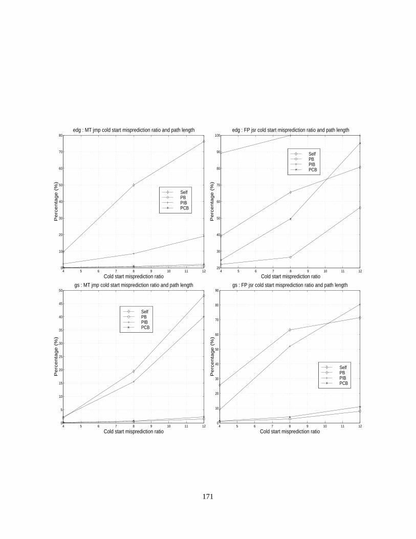
4 5 6 7 8 9 10 11 120

10

20

30

40

50

60

70

80edg : MT jmp cold start misprediction ratio and path length

Pe

rce

nta

ge

(%

)


SelfPBPIBPCB

4 5 6 7 8 9 10 11 1220

30

40

50

60

70

80

90

100edg : FP jsr cold start misprediction ratio and path length

Pe

rce

nta

ge

(%

)


SelfPBPIBPCB

4 5 6 7 8 9 10 11 120

5

10

15

20

25

30

35

40

45

50gs : MT jmp cold start misprediction ratio and path length

Pe

rce

nta

ge

(%

)


SelfPBPIBPCB

4 5 6 7 8 9 10 11 120

10

20

30

40

50

60

70

80

90gs : FP jsr cold start misprediction ratio and path length

Pe

rce

nta

ge

(%

)


SelfPBPIBPCB

171

4 5 6 7 8 9 10 11 120

5

10

15

20

25

30

35

40

45troff : MT jmp cold start misprediction ratio and path length

Pe

rce

nta

ge

(%

)


SelfPBPIBPCB

4 5 6 7 8 9 10 11 1210

20

30

40

50

60

70

80

90

100troff : FP jsr cold start misprediction ratio and path length

Pe

rce

nta

ge

(%

)


SelfPBPIBPCB

4 5 6 7 8 9 10 11 120

5

10

15

20

25

30

35troff : VF jsr cold start misprediction ratio and path length

Pe

rce

nta

ge

(%

)


SelfPBPIBPCB

4 5 6 7 8 9 10 11 120

5

10

15

20

25

30

35eqn : MT jmp cold start misprediction ratio and path length

Pe

rce

nta

ge

(%

)


SelfPBPIBPCB

4 5 6 7 8 9 10 11 1299

99.2

99.4

99.6

99.8

100

100.2

100.4

100.6

100.8

101eqn : FP jsr cold start misprediction ratio and path length

Pe

rce

nta

ge

(%

)


SelfPBPIBPCB

4 5 6 7 8 9 10 11 120

10

20

30

40

50

60

70

80eqn : VF jsr cold start misprediction ratio and path length

Pe

rce

nta

ge

(%

)


SelfPBPIBPCB

172

4 5 6 7 8 9 10 11 120

5

10

15

20

25

30

35

40

45

50bore : MT jmp cold start misprediction ratio and path length

Pe

rce

nta

ge

(%

)


SelfPBPIBPCB

4 5 6 7 8 9 10 11 120

2

4

6

8

10

12

14

16

18

20bore : FP jsr cold start misprediction ratio and path length

Pe

rce

nta

ge

(%

)


SelfPBPIBPCB

4 5 6 7 8 9 10 11 120

10

20

30

40

50

60

70bore : VF jsr cold start misprediction ratio and path length

Pe

rce

nta

ge

(%

)


SelfPBPIBPCB

4 5 6 7 8 9 10 11 120

5

10

15

20

25

30

35

40

45porky : MT jmp cold start misprediction ratio and path length

Pe

rce

nta

ge

(%

)


SelfPBPIBPCB

4 5 6 7 8 9 10 11 120

2

4

6

8

10

12

14

16

18

20porky : FP jsr cold start misprediction ratio and path length

Pe

rce

nta

ge

(%

)


SelfPBPIBPCB

4 5 6 7 8 9 10 11 120

10

20

30

40

50

60

70porky : VF jsr cold start misprediction ratio and path length

Pe

rce

nta

ge

(%

)


SelfPBPIBPCB

173

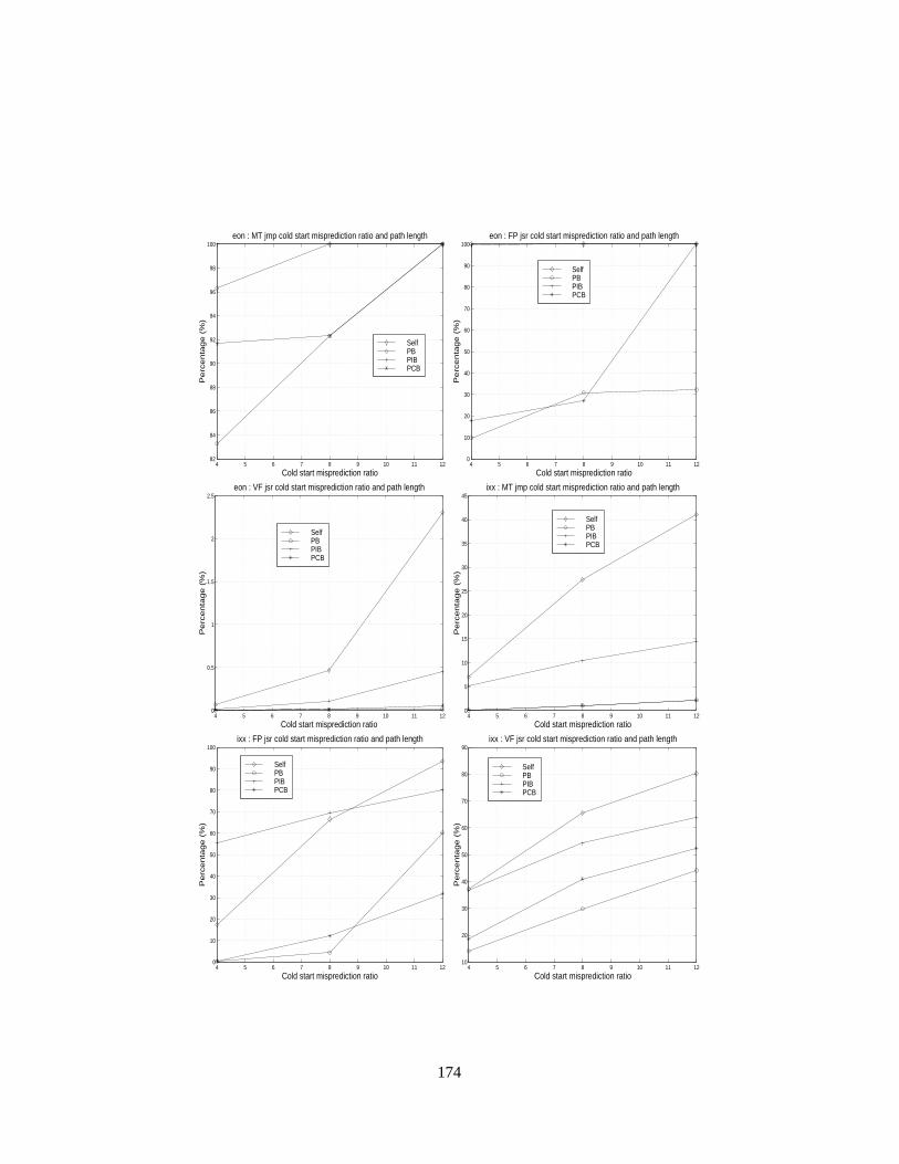
4 5 6 7 8 9 10 11 1282

84

86

88

90

92

94

96

98

100eon : MT jmp cold start misprediction ratio and path length

Pe

rce

nta

ge

(%

)


SelfPBPIBPCB

4 5 6 7 8 9 10 11 120

10

20

30

40

50

60

70

80

90

100eon : FP jsr cold start misprediction ratio and path length

Pe

rce

nta

ge

(%

)


SelfPBPIBPCB

4 5 6 7 8 9 10 11 120

0.5

1

1.5

2

2.5eon : VF jsr cold start misprediction ratio and path length

Pe

rce

nta

ge

(%

)


SelfPBPIBPCB

4 5 6 7 8 9 10 11 120

5

10

15

20

25

30

35

40

45ixx : MT jmp cold start misprediction ratio and path length

Pe

rce

nta

ge

(%

)


SelfPBPIBPCB

4 5 6 7 8 9 10 11 120

10

20

30

40

50

60

70

80

90

100ixx : FP jsr cold start misprediction ratio and path length

Pe

rce

nta

ge

(%

)


SelfPBPIBPCB

4 5 6 7 8 9 10 11 1210

20

30

40

50

60

70

80

90ixx : VF jsr cold start misprediction ratio and path length

Pe

rce

nta

ge

(%

)


SelfPBPIBPCB

174

4 5 6 7 8 9 10 11 120

10

20

30

40

50

60

70

80lcom : MT jmp cold start misprediction ratio and path length

Pe

rce

nta

ge

(%

)


SelfPBPIBPCB

4 5 6 7 8 9 10 11 1298.5

99

99.5

100lcom : FP jsr cold start misprediction ratio and path length

Pe

rce

nta

ge

(%

)


SelfPBPIBPCB

4 5 6 7 8 9 10 11 120

10

20

30

40

50

60

70

80

90lcom : VF jsr cold start misprediction ratio and path length

Pe

rce

nta

ge

(%

)


SelfPBPIBPCB

175

Appendix C

The following plots present the dynamic count of conditional and indirect branches as well as their mispredicted

population. A data point is recorded for every 500 cycles of machine execution time. Data are plotted for the

edg and perl benchmarks and correspond to the selected simulation intervals. Both edg and perl were run until

300M of instructions were committed. An additional 350M were executed before statistics were recorded (for

perl only). Three different sets of plots are listed for eachbenchmark. The first one corresponds to the activity

of a machine with no indirect branch prediction and the conservative fetch unit described in chapter 5 while

the other two utilize the PPM predictor with a conservative or an aggressive fetch unit. More details about the

fetch unit models can be found in chapter 5.

176

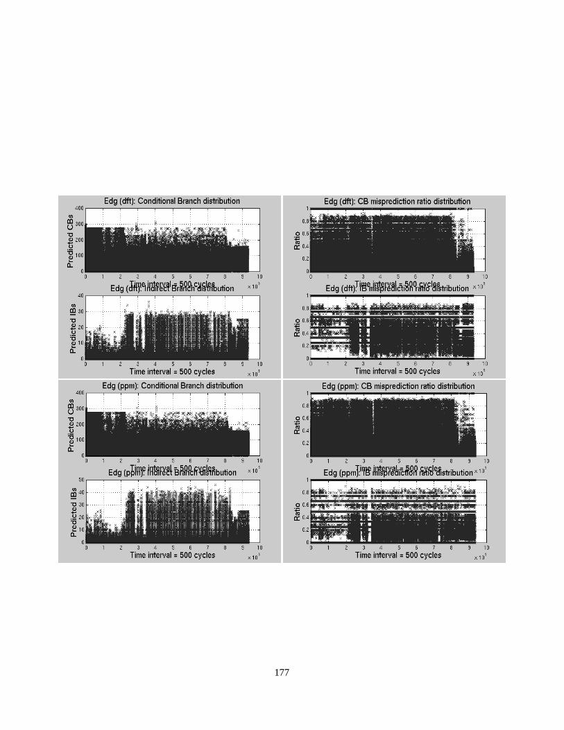
177

178

179

Appendix D

The following figures show the average occupancy for the I-fetch queue and the centralized instruction window

of the processor configurations with and without indirect branch prediction. Statistics are presented for both

fetch models in number of instructions. Theaf acronym signifies an aggressive I-fetch model.

180

0 5 10 15 20 25 30 35

Dft

BTB

BTB2b

GAg

Dpath

Cascade

PPM

afDft

afBTB

afBTB2b

afGAg

afDpath

afCascade

afPPM

Gcc: Instruction window occupancy with IB predictors

insns0 10 20 30 40 50

Dft

BTB

BTB2b

GAg

Dpath

Cascade

PPM

afDft

afBTB

afBTB2b

afGAg

afDpath

afCascade

afPPM

Perl: Instruction window occupancy with IB predictors

insns

0 2 4 6 8 10 12 14 16 18

Dft

BTB

BTB2b

GAg

Dpath

Cascade

PPM

afDft

afBTB

afBTB2b

afGAg

afDpath

afCascade

afPPM

Edg: Instruction window occupancy with IB predictors

insns0 5 10 15 20 25 30 35 40 45

Dft

BTB

BTB2b

GAg

Dpath

Cascade

PPM

afDft

afBTB

afBTB2b

afGAg

afDpath

afCascade

afPPM

Ixx: Instruction window occupancy with IB predictors

insns

0 5 10 15 20 25 30 35 40

Dft

BTB

BTB2b

GAg

Dpath

Cascade

PPM

afDft

afBTB

afBTB2b

afGAg

afDpath

afCascade

afPPM

Troff: Instruction window occupancy with IB predictors

insns0 5 10 15 20 25 30 35 40 45

Dft

BTB

BTB2b

GAg

Dpath

Cascade

PPM

afDft

afBTB

afBTB2b

afGAg

afDpath

afCascade

afPPM

Eqn: Instruction window occupancy with IB predictors

insns

181

0 2 4 6 8 10 12 14

Dft

BTB

BTB2b

GAg

Dpath

Cascade

PPM

afDft

afBTB

afBTB2b

afGAg

afDpath

afCascade

afPPM

Gcc: IFQ occupancy with IB predictors

Ifq occupancy (insns)0 5 10 15 20 25

Dft

BTB

BTB2b

GAg

Dpath

Cascade

PPM

afDft

afBTB

afBTB2b

afGAg

afDpath

afCascade

afPPM

Perl: IFQ occupancy with IB predictors


0 1 2 3 4 5 6 7

Dft

BTB

BTB2b

GAg

Dpath

Cascade

PPM

afDft

afBTB

afBTB2b

afGAg

afDpath

afCascade

afPPM

Edg: IFQ occupancy with IB predictors

Ifq occupancy (insns)0 5 10 15 20

Dft

BTB

BTB2b

GAg

Dpath

Cascade

PPM

afDft

afBTB

afBTB2b

afGAg

afDpath

afCascade

afPPM

Ixx: IFQ occupancy with IB predictors


0 2 4 6 8 10 12 14 16 18

Dft

BTB

BTB2b

GAg

Dpath

Cascade

PPM

afDft

afBTB

afBTB2b

afGAg

afDpath

afCascade

afPPM

Troff: IFQ occupancy with IB predictors

Ifq occupancy (insns)0 5 10 15 20

Dft

BTB

BTB2b

GAg

Dpath

Cascade

PPM

afDft

afBTB

afBTB2b

afGAg

afDpath

afCascade

afPPM

Eqn: IFQ occupancy with IB predictors


182

Bibliography

[1] A. Tannenbaum. Implications of Structured Programmingfor Machine Architecture.Communications of the ACM, 21(3):237–

246, March 1978.

[2] Manolis Katevenis.Reduced Instruction Set Computer Architecture for VLSI. MIT Press, 1985.

[3] D. Knuth. An Empirical Study of FORTRAN Programs.Software, Practice and Experience, (1):105–133, 1971.

[4] J. Elshoff. A Numerical Profile of Commercial PL/1 Programs. Software, Practice and Experience, (6):505–525, 1976.

[5] John Hennessy and David Patterson.Computer Architecture : a Quantitative approach. Morgan Kaufman Publishers, 1990.

[6] Robert Colwell. The Performance Effects of Functional Migration and Architectural Complexity in Object-Oriented Systems.

PhD thesis, Carnegie-Mellon University, 1985.

[7] A. Silbey, V. Milutinovic, and V. Mendoza-Grado. A Survey of Advanced Microprocessors and HLL Computer Architectures.

IEEE Computer, pages 72–85, August 1986.

[8] D.W. Anderson, F.J. Sparacio, and R.M. Tomasulo. The IBMSystem/360 model 91: Machine Philosophy and Instruction

Handling. IBM Journal of Research and Development, 11:8–24, January 1967.

[9] R. Giladi and N. Ahituv. SPEC as a Performance EvaluationMeasure.IEEE Computer, 28(8):33–42, August 1995.

[10] David M. Ungar.The Design and Evaluation of a High Performance Smalltalk System. MIT Press, 1987.

[11] A. Singhal and Y.N. Patt. A High Performance Prolog Processor with Multiple Functional Units. InProceedings of the Interna-

tional Symposium on Architecture, pages 195–202, May 1989.

[12] B.J. Cox.Object-Oriented Programming. Addison-Wesley, 1987.

[13] B. Calder, D. Grunwald, and B. Zorn. Quantifying Behavioral Differences between C and C++ programs.Journal of Program-

ming Languages, 2(4):313–351, January 1994.

[14] D. Detlefs, A. Dosser, and B. Zorn. Memory Allocation Costs in large C and C++ Programs.Software, Practice and Experience,

24(6):527–542, 1994.

[15] R. Henderson and B. Zorn. A Comparison of Object-Oriented Programming in four Modern Languages.Software, Practice and

Experience, 24(11):1077–1095, November 1994.

[16] R. Radhakrishan and L. John. Execution Characteristics of Object Oriented Programs on the UltraSparc-II. InProceedings of

the International High Performance Computing Conference, December 1998.

[17] D.C.D. Tang, A.M. Grizzaffi Maynard, and L. John. Contrasting Branch Characteristics and Branch Predictor Performance of

C++ and C Programs. InProceedings of the IEEE Performance, Computers and Communications Conference, February 1999.

[18] Urs Holzle and David Ungar. Do Object-Oriented Languages need Special Hardware Support? InProceedings of the 9th

European Conference on Object-Oriented Programming, pages 253–282, August 1995.

183

[19] O. Agesen and U. Holzle. Type Feedback vs. Concrete TypeInference: A Comparison of Optimization Techniques for Object-

Oriented Languages. InProceedings of the 10th Conference on Object-Oriented Programming, Systems, Languages and Appli-

cations, pages 91–107, October 1995.

[20] G. Aigner and U. Holzle. Eliminating Virtual Function Calls in C++ Programs. InProceedings of the 10th European Conference

on Object-Oriented Programming, pages 142–166, July 1996.

[21] C. Chambers and D. Ungar. Iterative Type Analysis and Extended Message Splitting : Optimizing Dynamically-Typed Object-

Oriented Programs. InProceedings of the International Conference on Programming Language Design and Implementation,

pages 150–165, June 1990.

[22] Jeffrey Dean, David Grove, and Craig Chambers. Optimization of Object-Oriented Programs using Static Class Hierarchy

Analysis. InProceedings of the 9th European Conference on Object-Oriented Programming, pages 77–101, August 1995.

[23] Mary Fernandez. Simple and Effective Link-Time Optimization of Modula-3 Programs. InProceedings of the International

Conference on Programming Language Design and Implementation, pages 103–115, June 1995.

[24] Urs Holzle and David Ungar. Optimizing Dynamically-Dispatched Calls with Run-Time Type Feedback. InProceedings of the

International Conference on Programming Language Design and Implementation, pages 326–336, June 1994.

[25] John Plevyak and Andrew Chien. Compilation of Object-Oriented Programming Languages. Technical Report Submitted for

publication, University of Illinois, Urbana-Champaign, October 1995.

[26] Mario Wolczko and Ifor Williams. The Influence of the Object-Oriented Language Model on a Supporting Architecture.In

Proceedings of the Hawaii International Conference on System Sciences, pages 182–191, January 1993.

[27] Emdad Khan, Mansoor Al-A’ali, and Moheb Girgis. ObjectOriented Programming for Structural Procedural Programmers.

IEEE Computer Magazine, 28(10):48–57, October 1995.

[28] Bjarne Stroustrup.The C++ Programming Language. Addison Wesley, 2nd edition edition, 1991.

[29] Amitabh Srivastava. Unreachable Procedures in Object-Oriented Programming.ACM Letters on Programming Languages and

Systems, 1(4):355–364, December 1992.

[30] P. Sweeney and F. Tip. A Study of Dead Data Members in C++ Applications. Technical Report RC-21051, IBM T.J. Watson

Center, July 1997.

[31] K. Driesen. Software and Hardware Techniques for Efficient PolymorphicCalls. PhD thesis, University of California, Santa

Barbara, 1999.

[32] J. Davidson and A.M. Holler. Subprogram Inlining: A Study of its Effects on Program Execution Time.IEEE Transactions on

Software Engineering, 18(2):89–101, February 1992.

[33] Jeffrey Dean, Craig Chambers, and David Grove. Selective Specialization for Object-Oriented Languages. InProceedings of

the International Conference on Programming Language Design and Implementation, pages 93–102, June 1995.

[34] D. Grove, G. DeFouw, J. Dean, and C. Chambers. Call GraphConstruction in Object-Oriented Languages. InProceedings of

the Conference on Object-Oriented Programming, Systems, Languages and Applications, pages 108–124, October 1997.

[35] D.R. Kaeli and P.G. Emma. Branch History Table Prediction of moving Target Branches due to Subroutine Returns. In

Proceedings of the International Symposium on Computer Architecture, pages 34–42, May 1991.

[36] D. Barrett and B. Zorn. Using Lifetime Predictors to Improve Memory Allocation Performance. InProceedings of the Interna-

tional Conference on Programming Language Design and Implementation, pages 187–196, June 1993.

[37] M. Seidl and B. Zorn. Segregating Heap Objects by Reference Behavior and Lifetime. InProceedings of the International

Conference for Programming Languages and Operating Systems, October 1998.

184

[38] D. Grunwald, B. Zorn, and R. Henderson. Improving the Cache Locality of Memory Allocation. InProceedings of the Interna-

tional Conference on Programming Language Design and Implementation, pages 177–186, June 1993.

[39] Hemand Pande and Barbara Ryder. Static Type Determination and Aliasing for C++. Technical Report LCSR-TR-250-A,

Rutgers University, October 1995.

[40] S.B. Lippman.Inside the C++ Object Model. Addison Wesley, 1996.

[41] P. Deutch and A. Schiffman. Efficient Implementation ofthe Smalltalk-80 System. InProceedings of the 11th Symposium on

the Principles of Programming Languages, 1984.

[42] Harini Srinivasan and Peter Sweeney. Evaluating Virtual Dispatch Mechanisms for C++. Technical Report RC 20330, IBM T.J.

Watson Center, January 1996.

[43] K. Driesen, U. Holzle, and J. Vitek. Message Dispatch inPipelined Processors. InProceedings of the 9th European Conference

on Object-Oriented Programming, pages 253–282, August 1995.

[44] K. Driesen and U. Holzle. The Direct Cost of Virtual Function Calls in C++. InProceedings of the 12th Conference on

Object-Oriented Programming, Systems, Languages and Applications, pages 306–323, October 1996.

[45] David Ungar and Randall Smith. SELF : The Power of Simplicity. In Proceedings of the 2nd Conference on Object-Oriented

Programming, Systems, Languages and Applications, pages 227–241, October 1987.

[46] D. Burger, J. Goodman, and A. Kagi. Memory Bandwidth Limitations of Future Microprocessors. InProceedings of the

International Symposium on Computer Architecture, pages 78–89, May 1996.

[47] M.D. Hill. Aspects of Cache Memory and Instruction Buffer Performance. PhD thesis, University of California, Berkeley, 1987.

[48] C.H. Chi and H. Dietz. Improving Cache Performance withSelective Cache Bypass. InProceedings of the Hawaii International

Conference on System Sciences, pages 277–285, January 1989.

[49] A. Anarwal and S.D. Pudar. Column Associative Caches : Atechnique for Reducing the Miss Rate of Direct-Mapped Caches.

In Proceedings of the International Symposium on Computer Architecture, pages 179–190, May 1993.

[50] S. Abraham and H. Agusleo. Reduction of Cache Interference Misses through Selective Bit-Permutation Mapping. Technical

Report CSE-TR-205-94, University of Michigan, Ann Arbor, 1994.

[51] A. Gonzalez, M. Valero, N. Topham, and J. Parcerisa. Eliminating Cache Conflict Misses through XOR-based Placement

Functions. InProceedings of International Conference on Supercomputing, pages 76–83, July 1997.

[52] A.H. Hashemi, D. R.Kaeli, and B. Calder. Efficient Procedure Mapping using Cache Line Coloring. InProceedings of the

International Conference on Programming Language Design and Implementation, pages 171–182, June 1997.

[53] S. McFarling. Program Optimization for Instruction Caches. InProceedings of the International Symposium on Architectural

Support for Programming Languages and Operating Systems, pages 183–191, April 1989.

[54] K. Pettis and R. Hansen. Profile-Guided Code Positioning. In Proceedings of the International Conference on Programming

Language Design and Implementation, pages 16–27, June 1990.

[55] N. Gloy, T. Blackwell, M.D. Smith, and B. Calder. Procedure Placement using Temporal Ordering Information. InProceedings

of the International Symposium on Microarchitecture, pages 303–313, December 1997.

[56] Mike Johnson.Superscalar Microprocessor Design. Prentice Hall, 1990.

[57] J.E. Smith and G. Sohi. The Microarchitecture of Superscalar Processors.Proceedings of the IEEE, 83(12):1609–1624, Decem-

ber 1995.

[58] J.E. Smith. A Study of Branch Prediction Strategies. InProceedings of the International Conference on Computer Architecture,

pages 135–148, May 1981.

185

[59] Digital Equipment Corporation, Maynard, Massachusetts. ATOM User Manual, March 1994.

[60] A. Srivastava and A. Eustace. ATOM : A System for Building Customized Program Analysis tools. InProceedings of the

International Conference on Programming Language, Designand Implementation, pages 196–205, June 1994.

[61] D. Burger and T. Austin. The SimpleScalar Tool Set, v2.0. Technical Report UW-CS-97-1342, University of Winsconsin,

Madison, June 1997.

[62] B. Bershad, D. Lee, T. Romer, and J.B. Chen. Avoiding Conflict Misses Dynamically in Large Direct-Mapped Caches. In

Proceedings of the International Conference on Architectural Support for Programming Languages and Operating Systems,

pages 158–170, October 1994.

[63] K. Harty and D.R. Cheriton. Application-controlled Physical Memory using External Page Cache Management. InProceedings

of the International Conference on Architectural Support for Programming Languages and Operating Systems, pages 187–197,

October 1992.

[64] R. Kessler and M. Hill. Page Placement Algorithms for Large Real Indexed Caches.ACM Transactions on Computer Systems,

10(4):338–359, November 1992.

[65] T. Sherwood, B. Calder, and J. Emer. Reducing Cache Misses using Hardware and Software Page Placement. InProceedings of

the International Conference on Supercomputing, June 1999.

[66] W.M. Hwu and P.P. Chang. Achieving High Instruction Cache Performance with an Optimizing Compiler. InProceedings of

the International Symposium on Computer Architecture, pages 242–251, May 1989.

[67] R. Cohn, D. Goodwin, and P.G. Lowney. Optimizing Alpha Executables on Windows NT with Spike.Digital Technical Journal,

9(4):3–20, 1997.

[68] J. Kalamatianos and D.R. Kaeli. Temporal-Based Procedure Reordering for Improved Instruction Cache Performance. In

Proceedings of the International Conference on High Performance Computer Architecture, pages 244–253, February 1998.

[69] B. Calder and D. Grunwald. Reducing Branch Costs via Branch Alignment. InProceedings of the International Conference on

Architectural support for programming languages and operating systems, pages 242–251, October 1994.

[70] C. Young and D.S. Johnson et.al. Near-Optimal Intraprocedural Branch Alignment. InProceedings of the International Confer-

ence on Programming Language Design and Implementation, pages 183–193, June 1997.

[71] M. Katevenis and N. Tzartzanis. Reducing the Branch Penalty by Rearranging Instructions in a Double-Width Memory.In

Proceedings of the International Conference on Architectural support for programming languages and operating systems, pages

15–27, April 1991.

[72] J. Torrellas, C. Xia, and R. Daigle. Optimizing the Instruction Cache Performance of an Operating System.IEEE Transactions

on Computers, 47(12):1363–1381, December 1998.

[73] J. Torrellas, C. Xia, and R. Daigle. Optimizing Instruction Cache Performance for Operating System Intensive Workloads. In

Proceedings of the International Conference on High Performance Computer Architecture, pages 360–369, January 1995.

[74] R. Cohn and P.G. Lowney. Hot Cold Optimizations of LargeWindows/NT Applications. InProceedings of the International

Symposium on Microarchitecture, pages 80–89, December 1996.

[75] J. Fisher. Trace Scheduling: A Technique for Global Microcode Compaction.IEEE Transactions on Computers, 30(7):478–490,

July 1981.

[76] K.Gosmann and C.Hafer et.al. Code Reorganization for Instruction Caches. InProceedings of the Hawaii International Con-

ference on System Sciences, pages 214–223, January 1993.

[77] Dennis Lee. Instruction Cache Effects of different Code Reordering Algorithms. Technical Report FR-35, University of Wash-

ington, Seattle, October 1994.

186

[78] A.H. Hashemi, D. R.Kaeli, and B. Calder. Procedure Mapping using Static Call Graph Estimation. InProceedings of the

Workshop on Interaction between Compiler and Computer Architecture, February 1997.

[79] A. Mendlson, S. Pinter, and R. Shtokhamer. Compile-Time Instruction Cache Optimizations. InProceedings of the International

Conference on Compiler Construction, pages 404–418, April 1994.

[80] R.R. Heisch. Trace-Directed Program Restructuring for AIX Executables. IBM Journal of Research and Development,

38(5):595–603, September 1994.

[81] J.B. Chen and B.D.D. Leupen. Improving Instruction Locality with Just-In-Time Code Layout. InProceedings of the UNENIX

Windows NT Workshop, August 1997.

[82] D.J. Scales. Efficient Dynamic Procedure Placement. Technical Report WRL-98/5, Compaq WRL Research Lab, May 1998.

[83] W. Chen, P.P. Chang, T. Conte, and W.W. Hwu. The Effect ofCode Expanding Optimizations on Instruction Cache Design.

IEEE Transactions on Computers, 42(9):1045–1057, September 1993.

[84] I. Bahar, B. Calder, and D. Grunwald. A Comparison of Software Code Reordering and Victim Buffers. InProceedings of the

International Workshop on the Interaction between Compilers and Computer Architecture, October 1998.

[85] A. Ramirez, J. Larriba-Pey, C. Navarro, and et.al. Software Trace Cache. InProceedings of the International Conference on

Supercomputing, June 1999.

[86] W.M. Hwu and P.P. Chang. Trace Selection for compiling Large C Application Programs to Microcode. InProceedings of the

International Workshop on Microarchitecture and Microprogramming, November 1988.

[87] E. Rotenberg, S. Bennett, and J. Smith. Trace Cache: A Low Latency Approach to High Bandwidth Instruction Fetching.In

Proceedings of the International Symposium on Microarchitecture, pages 24–35, December 1996.

[88] Barbara Ryder. Constructing the Call Graph of a Program. IEEE Transactions on Software Engineering, 5(3):216–226, 1979.

[89] D. Wall. Predicting Program Behavior using Real or Estimated Profiles. InProceedings of the International Conference on

Programming Language Design and Implementation, pages 59–70, June 1991.

[90] G. Ammons, T. Ball, and J. Larus. Exploiting Hardware Performance Counters with Flow and Context Sensitive Profiling. In

Proceedings of the International Conference on Programming Language Design and Implementation, pages 85–96, June 1997.

[91] J. Kalamatianos, A. Khalafi, D.R. Kaeli, and W. Meleis. Analysis of Temporal-based Program Behavior for Improved Instruction

Cache Performance.IEEE Transactions on Computers, 48(2):168–175, February 1999.

[92] T. Rollins and B. Strecker. Use of the LRU Stack Depth Distribution for Simulation of Paging Behavior.Communications of the

ACM, 20(7):795–798, November 1977.

[93] P. Denning. The Working Set Model for Program Behavior.Communications of the ACM, 11(5):323–333, May 1968.

[94] G. Shedler and C. Tung. Locality in Page Reference Strings. SIAM Journal of Computing, 1(3), September 1976.

[95] V.Phalke and B.Gopinath. An Inter-Reference Gap Modelfor Temporal Locality in Program Behavior. InProceedings of the

International Conference on Measuring and Modeling Computer Systems, pages 291–300, May 1995.

[96] R. Quong. Expected I-Cache Miss Rates via the Gap Model.In Proceedings of the International Symposium on Computer

Architecture, pages 372–383, April 1994.

[97] A. Mendelson, D. Thiebaut, and D. Pradhan. Modeling Live and Dead Lines in Cache Memory Systems.IEEE Transactions on

Computers, 42(1):1–14, January 1993.

[98] V. Phalke and B. Gopinath. Compression-based Program Characterization for Improving Cache Memory Performance.IEEE

Transactions on Computers, 46(11):1187–1201, November 1997.

187

[99] N. Gloy and M. Smith. Procedure Placement using Temporal-Ordering Information. ACM Transactions on Programming

Languages and Systems, 21:111–164, 1999.

[100] T. Ball and J. Larus. Efficient Path Profiling. InProceedings of the International Symposium on Microarchitecture, pages 46–57,

December 1996.

[101] T. Ball, P. Mataga, and M. Sagiv. Edge Profiling versus Path Profiling: The Showdown. InProceedings of the International

Symposium on Principles of Programming Languages, January 1998.

[102] R. Cohn and P.G. Lowney. Feedback Directed Optimizations in Compaq’s Compilation Tools for Alpha. InProceedings of the

2nd Workshop on Feedback-Directed Optimization, November 1999.

[103] N. Gloy. Code Placement using Temporal Profile Information. PhD thesis, Harvard University, 1998.

[104] J. Pierce and T. Mudge. The Effect of Speculative Execution on Cache Performance. InProceedings of the International Parallel

Processing Symposium, April 1994.

[105] P.Y. Chang, E. Hao, T.Y. Yeh, and Y. Patt. Branch Classification : a New Mechanism for Improving Branch Predictor Perfor-

mance. InProceedings of the International Symposium on Microarchitecture, pages 22–31, December 1994.

[106] P.Y. Chang.Classification-Directed Branch Predictor Design. PhD thesis, University of Michigan, Ann Arbor, 1997.

[107] S. McFarling. Combining Branch Predictors. Technical Report TN-36, DEC WRL, June 1993.

[108] K. Driesen and U. Holzle. Accurate Indirect Branch Prediction. In Proceedings of the International Symposium on Computer

Architecture, pages 167–178, June 1998.

[109] K. Driesen and U. Holzle. Limits of Indirect Branch Prediction. Technical Report TRCS97-10, University of California, Santa

Barbara, June 1997.

[110] David Grove, Jeffrey Dean, Charles Garrett, and CraigChambers. Profile-Guided Receiver Class Prediction. InProceedings of

the 10th Conference on Object-Oriented Programming, Systems, Languages and Applications, pages 108–123, October 1995.

[111] B.C. Cheng and W.W. Hwu. An Empirical Study of FunctionPointers using SPEC Benchmarks. Technical Report TR-99-02,

University of Illinois, Urbagna-Champaign, May 1999.

[112] A. Shah and B.G. Ryder. Function Pointers in C - An Empirical Study. Technical Report LCSR-TR-244, Rutgers University,

May 1995.

[113] Digital Equipment Corporation, Maynard, Massachusetts. DEC OSF/1 Programmer’s Guide, 1993.

[114] A. Srivastava and D.W. Wall. Link-Time Optimization of Address Calculation on a 64-bit Architecture. Technical Report RR

94/1, DEC WRL, February 1994.

[115] Digital Equipment Corporation, Maynard, Massachusetts. Using DEC C++ for DEC OSF/1 Systems, May 1995.

[116] M. Ellis and B. Stroustrup.C++ Annotated Reference Manual. Addison-Wesley, 1990.

[117] R. Bernstein. Producing Good Code for the Case Statement. Software, Practice & Experience, 15(10):1021–1024, October

1985.

[118] H.D. Pande and B.G. Ryder. Data Flow-Based Virtual Function Resolution. InProceedings of the 3rd International Symposium

on Static Analysis, pages 238–254, September 1996.

[119] P. Carini and H. Srinivasan. Flow-Sensitive Type Analysis for C++. Technical Report RC-20267, IBM T.J. Watson Center,

November 1995.

[120] B. Calder and D. Grunwald. Reducing Indirect FunctionCall Overhead in C++ Programs. InProceedings of the 21st Annual

Symposium on Principles of Programming Languages, pages 397–408, January 1994.

188

[121] A. Reinig. Alias Analysis in the DEC C and Digital C++ Compilers.Digital Technical Journal, 10(1):48–57, December 1998.

[122] B.C. Cheng and W.W. Hwu. A Practical Interprocedural Pointer Analysis Framework. Technical Report IMP-99-01, University

of Illinois, Urbagna-Champaign, April 1999.

[123] K. Wang and M. Franklin. Highly Accurate Data Value Prediction. In Proceedings of the International Conference on High

Performance Computing, pages 358–363, December 1997.

[124] S.T. Srinivasan and A.R. Lebeck. Load Latency Tolerance in Dynamically Scheduled Processors. InProceedings of the Inter-

national Symposium on Microarchitecture, pages 148–159, December 1998.

[125] J.K.F. Lee and A.J. Smith. Branch Prediction Strategies and Branch Target Buffer Design.IEEE Computer Magazine, 17(1):6–

22, January 1984.

[126] C.H. Perleberg and A.J. Smith. Branch Target Buffer Design and Optimization.IEEE Transactions on Computers, 42(4):396–

412, April 1993.

[127] K. Skadron, P. Ahuja, M. Martonosi, and D. Clark. Improving Prediction for Procedure Returns with Return-Address-Stack

Repair Mechanisms. InProceedings of the International Symposium on Microarchitecture, pages 259–271, December 1998.

[128] S. Jourdan, T.H. Hsing, J. Stark, and Y.N. Patt. The Effects of Mispredicted Path Execution on Branch Prediction Structures.

In Proceedings of the International Conference on Parallel Architectures and Compilation Techniques, pages 58–67, October

1996.

[129] D.R. Kaeli and P.G. Emma. Improving the Accuracy of History-based Branch Prediction.IEEE Transactions on Computers,

46(4):469–472, April 1997.

[130] P.Y. Chang, E. Hao, and Y. Patt. Target Prediction for Indirect Jumps. InProceedings of the International Symposium on

Computer Architecture, pages 274–283, June 1997.

[131] T.Y. Yeh and Y. Patt. Two-Level Adaptive Training Branch Prediction. InProceedings of the International Symposium on

Microarchitecture, pages 51–61, November 1991.

[132] K. Driesen and U. Holzle. The Cascaded Predictor: Economic and Adaptive Branch Target Prediction. InProceedings of the

31st International Symposium on Microarchitecture, November 1998.

[133] J. Stark, M. Evers, and Y. Patt. Variable Length Path Branch Prediction. InProceedings of the International Conference on

Programming Languages and Operating Systems, pages 170–179, October 1998.

[134] A. Roth, A. Moshovos, and G. Sohi. Improving Virtual Function Call Target Prediction via Dependence-based Pre-Computation.

In Proceedings of the International Conference on Supercomputing, June 1999.

[135] T.C. Bell, J.G. Cleary, and I.H. Witten.Text Compression. Prentice Hall, 1990.

[136] M. Feder, N. Merhav, and M. Gutman. Universal Prediction of Individual Sequences.IEEE Transactions on Information Theory,

pages 1258–1270, July 1992.

[137] A. Moffat. Implementing the PPM Data Compression Scheme. IEEE Transactions on Communications, 38(11):1917–1921,

November 1990.

[138] J.G. Cleary and I.H. Witten. Data Compression using Adaptive Coding and Partial String Machines.IEEE Transactions on

Communications, 32(4):396–402, April 1984.

[139] F. Willems, Y. Shtarkov, and T. Tjalkens. The Context Tree Weighting Method: Basic Properties.IEEE Transactions on

Information Theory, 41(3), May 1995.

[140] E. Federovksy, M. Feder, and S. Weiss. Branch Prediction based on Universal Data Compression Algorithms. InProceedings

of the International Symposium on Architecture, pages 62–72, June 1998.

189

[141] I.C.K. Chen, J.T. Coffey, and T.N. Mudge. Analysis of Branch Prediction via Data Compression. InProceedings of the

International Conference on Architectural support for programming languages and operating systems, pages 128–137, October

1996.

[142] T.M. Kroeger and D.D. Long. Predicting File System Actions from Prior Events. InProceedings of the USENIX Winter Technical

Conference, January 1996.

[143] Y. Sazeides and J.E. Smith. Implementations of Context-based Value Predictors. Technical Report TR-ECE-97-8, University of

Winsconsin, Madison, December 1997.

[144] B. Calder and D. Grunwald. Fast and Accurate Instruction Fetch and Branch Prediction. InProceedings of the International

Symposium on Computer Architecture, pages 2–11, April 1994.

[145] J. Kalamatianos and D.R. Kaeli. Predicting Indirect Branches via Data Compression. InProceedings of the International

Symposium on Microarchitecture, pages 272–281, December 1998.

[146] A. Moshovos, S. Breach, T.N. Vijaykumar, and G. Sohi. Dynamic Speculation and Synchronization of Data Dependences. In

Proceedings of the International Symposium on Computer Architecture, June 1997.

[147] R. Sites and R. Witek.Alpha AXP Architecture Reference Manual. Digital Press, 1995.

[148] C.Y. Fu, M. Jennings, S. Larin, and T. Conte. Value Speculation Scheduling for High Performance Processors. InProceedings

of the International Conference on Architectural Support for Programming Languages and Operating Systems, October 1998.

[149] A. Rogers and K. Li. Software Support for Speculative Loads. InProceedings of the International Conference on Architectural

Support for Programming Languages and Operating Systems, pages 38–50, October 1992.

[150] T. Conte, K. Menezes, and et.al. Optimization of Instruction Fetch Mechanisms for High Issue Rates. InProceedings of the

International Symposium on Computer Architecture, pages 333–344, June 1995.

[151] G. Sohi and M. Franklin. High Bandwidth Data Memory Systems for Superscalar Processors. InProceedings of the International

Conference on Architectural Support for Programming Languages and Operating Systems, pages 53–62, April 1991.

[152] A. Seznec, S. Jourdan, P. Sainrat, and P. Michaud. Multiple-Block Ahead Branch Predictors. InProceedings of the International

Conference on Architectural Support for Programming Languages and Operating Systems, pages 116–127, October 1996.

[153] T.Y. Yeh and Y. Patt. Branch History Table Indexing to prevent Pipeline Bubbles in Wide-Issue Superscalar Processors. In

Proceedings of the International Symposium on Microarchitecture, pages 164–175, December 1993.

[154] H. Kwak, B. Lee, and et. al. Effects of Multithreading on Cache Performance.IEEE Transactions on Computers, 48(2):176–184,

February 1999.

[155] D. Melski and T. Reps. Interprocedural Path Profiling.Technical Report TR-98-1382, University of Wisconsin, Madison,

September 1998.

[156] J.D. Collins and D. Tullsen. Hardware Identification of Cache Conflict Misses. InProceedings of the International Symposium

on Microarchitecture, November 1999.

[157] S. Carr, K. McKinley, and C.W. Tseng. Compiler Optimizations for Improving Data Locality. InProceedings of the International

Conference on Architectural Support for Programming Languages and Operating Systems, pages 252–262, October 1994.

[158] M. Lam, E. Rothberg, and M. Wolf. The Cache Performanceand Optimizations of Blocked Algorithms. InProceedings of

the International Conference on Architectural Support forProgramming Languages and Operating Systems, pages 63–74, April

1991.

[159] B. Calder, C. Krintz, S. John, and T. Austin. Cache-Conscious Data Placement. InProceedings of the International Conference

on Architectural Support for Programming Languages and Operating Systems, pages 139–149, October 1998.

190

[160] G. Rivera and C.W. Tseng. Eliminating Conflict Misses for High Performance Architectures. InProceedings of the International

Conference on Supercomputing, pages 353–360, July 1998.

[161] T. Chilimbi, B. Davidson, and J. Larus. Cache-Conscious Structure Definition. InProceedings of the International Conference

on Programming Language Design and Implementation, pages 13–24, May 1999.

[162] W. Lynch, B. Bray, and M. Flynn. The Effect of Page Allocation on Caches. InProceedings of the International Symposium on

Microarchitecture, pages 222–225, December 1992.

[163] T. Romer, D. Lee, B. Bershad, and J.B. Chen. Dynamic Page Mapping Policies for Cache Conflict Resolution on Standard

Hardware. InProceedings of the International Conference on Operating Systems Design and Implementation, pages 255–266,

November 1994.

[164] B. Calder and D. Grunwald. Next Cache Line and Set Prediction. InProceedings of the International Symposium on Computer

Architecture, pages 287–296, June 1995.

[165] M. Lipasti, C.B. Wilkerson, and J.P. Shen. Value Locality and Load Value Prediction. InProceedings of the International

Conference on Architectural Support for Programming Languages and Operating Systems, October 1996.

191

Documents

NORTHEASTERN UNIVERSITY · Northeastern University Boston, Massachusetts September 2000. Abstract Applications, and their associated programming models, have had a profound inﬂuence