Nonlinear Structural Analysis - InfoGraph

Nonlinear Structural Analysis

The description of program functions within this documentation should not be considered a warranty of product features.All warranty and liability claims arising from the use of this documentation are excluded.

InfoGraph® is a registered trademark of InfoGraph GmbH, Aachen, Germany. The manufacturer and product namesmentioned below are trademarks of their respective owners.

This documentation is copyright protected. Reproduction, duplication, translation or electronic storage of this document orparts thereof is subject to the written permission of InfoGraph GmbH.

InfoGraph® Software, version 21, uses Microsoft® MFC and Intel® MKL Libraries.

© InfoGraph GmbH, October 2021. All rights reserved.

Title image: Arched Bridge Maulbeerstrasse, BaselCourtesy of DB Netz AG, Brückenmessung- u. bewertung N.BIF, Germany

1

Contents

© InfoGraph GmbH, October 2021

Contents

Basics 1

Area of Application 1

Analysis Method 1

Finite Beam Elements 3

Section Analysis 4

Reinforced Concrete Beams 4

Stress-Strain-Curves for the Ultimate Limit State Check 5

Stress-Strain-Curves for the Serviceability Check 7

Torsional Stiffness 9

Check of the Limit Strains (Ultimat Limit State Check) 9

Automatic Reinforcement Increase (Ultimate Limit State Check) 9

Concrete Creep 10

Steel Beams 10

Beams of Free Material 11

Area Elements 11

Reinforced Concrete Area Elements 12

Area Elements of Steel and Free Material 14

Solid Elements 15

Prestressed Structures 16

Notes on Convergence Behavior 16

Analysis Settings 17

Examples 19

Flat Ceiling With Cantilever in State II 19

Crosscheck of Two Short-Term Tests 22

Reinforced Concrete Slab 22

Reinforced Concrete Frame 23

Prestressed Concrete Structure 24

Snap Through Problem of a Cylindrical Shell 27

References 28

1

Basics



Basics

Area of ApplicationThe analysis option Nonlinear analysis enables the determination of the internal forces and deformations of beam and shellstructures made of reinforced concrete and steel as well as stress states of solid elements according to bilinear material lawwhile considering geometric and physical nonlinearities. A distinction can be made between calculations with materialcharacteristics for the ultimate limit state or the serviceability limit state. Due to the considerable numerical complexity, itonly makes sense to use this program module for special problems.

Specifically, the following nonlinear effects can be taken into consideration:

• Equilibrium of the deformed system according to the second- or third order theory, if this has been activated for thecorresponding load case.

• Beams and area elements made of reinforced concrete according to DIN 1045, DIN 1045-1, OENORM B4700, SIA 262and EN 1992-1-1.

• Beams and area elements made of steel with bilinear stress-strain curve under consideration of the Huber-von Misesyield criterion and complete interaction with all internal forces.

• Beams, area and solid elements with bilinear stress-strain curve respectively yield criterion according to Raghava andindividually definable compressive and tensile strength.

• Compression-flexible beams.

• Beam and area element bedding with bilinear bedding curve perpendicular to and alongside the beam.

• Solid elements with bilinear bedding curve in the element coordinate system.

• Pressed steel layers in bond with concrete in beams can be considered with a bilinear stress-strain curve.

• Tendon groups in bond with concrete can be taken into account with a bilinear stress-strain curve.

• Prestressing without bond (only load) can also be simulated.

• Beams and area elements made of steel and reinforced concrete in case of fire according to EN 1992-1-2 and EN 1993-1-2 or beams made of timber in case of fire according to EN 1995-1-2 (see chapter 'Structural analysis for fire scenarios').

Analysis MethodThe analysis model used is based on the finite element method. To carry out a nonlinear system analysis, the standard beamelements are replaced internally with shear-flexible nonlinear beams with an increased displacement function. For thetreatment of area and volume structures nonlinear layer elements and solid elements are used. In contrast to the linearcalculation and in order to account for the nonlinear or even discontinuous properties of the structure, a finer subdivision isgenerally necessary. The program assumes that the actions defined in the load cases are weighted with the appropriatepartial safety factors.

Requirements

• The beams are assumed to be straight.

• The area elements are flat.

• Area and beam sections are constant for each element.

• The dimensions of the section are small compared with the other system dimensions.

• Shear deformations of beams are accounted for with a shear distortion that is constant across the section, meaning thesection remains plane after the deformation but is no longer perpendicular to the beam axis.

• The mathematical curvature is linearized (second-order theory).

• The load is slowly increased to its final value and does not undergo any deviation in direction as a result of the systemdeformation.

Equilibrium iteration

To solve the nonlinear system of equations, both the incremental Newton-Raphson method and the arc length method canbe used. In both methods, the tangential stiffness matrix is computed in each iteration depending on the current internalforce and deformation state. Alternatively, a constant stiffness matrix (linear stiffness method) can be used. Here, thestiffness matrix is computed only once at the beginning of the numerical simulation and in the following assumed to beconstant.

2



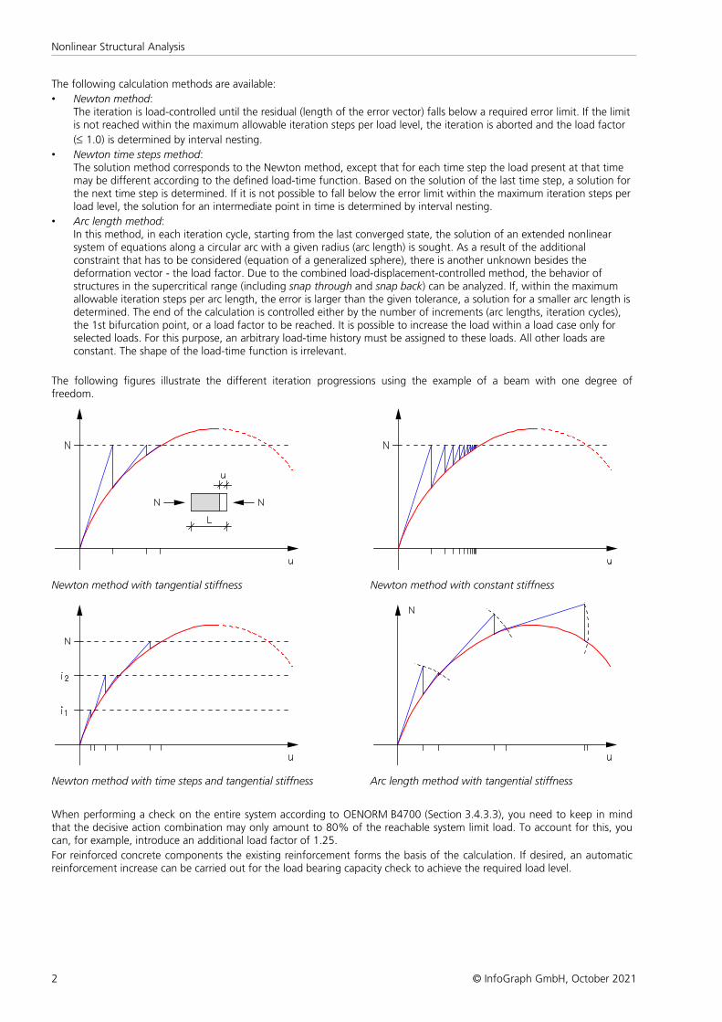
The following calculation methods are available:

• Newton method:The iteration is load-controlled until the residual (length of the error vector) falls below a required error limit. If the limitis not reached within the maximum allowable iteration steps per load level, the iteration is aborted and the load factor

(£ 1.0) is determined by interval nesting.

• Newton time steps method:The solution method corresponds to the Newton method, except that for each time step the load present at that timemay be different according to the defined load-time function. Based on the solution of the last time step, a solution forthe next time step is determined. If it is not possible to fall below the error limit within the maximum iteration steps perload level, the solution for an intermediate point in time is determined by interval nesting.

• Arc length method:In this method, in each iteration cycle, starting from the last converged state, the solution of an extended nonlinearsystem of equations along a circular arc with a given radius (arc length) is sought. As a result of the additionalconstraint that has to be considered (equation of a generalized sphere), there is another unknown besides thedeformation vector - the load factor. Due to the combined load-displacement-controlled method, the behavior ofstructures in the supercritical range (including snap through and snap back) can be analyzed. If, within the maximumallowable iteration steps per arc length, the error is larger than the given tolerance, a solution for a smaller arc length isdetermined. The end of the calculation is controlled either by the number of increments (arc lengths, iteration cycles),the 1st bifurcation point, or a load factor to be reached. It is possible to increase the load within a load case only forselected loads. For this purpose, an arbitrary load-time history must be assigned to these loads. All other loads areconstant. The shape of the load-time function is irrelevant.

The following figures illustrate the different iteration progressions using the example of a beam with one degree offreedom.

Newton method with tangential stiffness Newton method with constant stiffness

Newton method with time steps and tangential stiffness Arc length method with tangential stiffness

When performing a check on the entire system according to OENORM B4700 (Section 3.4.3.3), you need to keep in mindthat the decisive action combination may only amount to 80% of the reachable system limit load. To account for this, youcan, for example, introduce an additional load factor of 1.25.

For reinforced concrete components the existing reinforcement forms the basis of the calculation. If desired, an automaticreinforcement increase can be carried out for the load bearing capacity check to achieve the required load level.

3

Basics


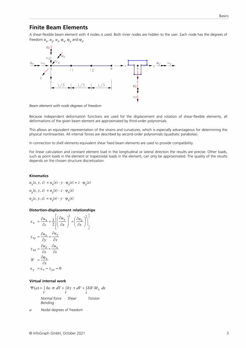
Finite Beam ElementsA shear-flexible beam element with 4 nodes is used. Both inner nodes are hidden to the user. Each node has the degrees of

freedom ux, uy, uz, jx, jy and jz.

Beam element with node degrees of freedom

Because independent deformation functions are used for the displacement and rotation of shear-flexible elements, alldeformations of the given beam element are approximated by third-order polynomials.

This allows an equivalent representation of the strains and curvatures, which is especially advantageous for determining thephysical nonlinearities. All internal forces are described by second-order polynomials (quadratic parabolas).

In connection to shell elements equivalent shear fixed beam elements are used to provide compatibility.

For linear calculation and constant element load in the longitudinal or lateral direction the results are precise. Other loads,such as point loads in the element or trapezoidal loads in the element, can only be approximated. The quality of the resultsdepends on the chosen structure discretization.

Kinematics

ux(x, y, z) = ux(x) - y · jz(x) + z · jy(x)

uy(x, y, z) = uy(x) - z · jx(x)

uz(x, y, z) = uz(x) - y · jx(x)

Distortion-displacement relationships

0

'

21

yzzy

x

xzxz

yxxy

2z

2yx

x

=g=e=e

¶

j¶=J

¶

¶+

¶

¶=g

¶

¶+

¶

¶=g

úú

û

ù

êê

ë

é÷ø

öçè

æ

¶

¶+÷

÷ø

öççè

æ

¶

¶+

¶

¶=e

x

z

u

x

u

x

u

y

u

x

u

x

uu

x

Virtual internal work

ò ò ×Jd+ò t×gd+s×ed=YV LV

dxMdVdVa x')(

Normal force Shear TorsionBending

a Nodal degrees of freedom

4



Tangential stiffness matrix

torsionshearTT

T K KdV d

dBσBdK

da

d

V

++÷ø

öçè

æ

e

s×+×==

Yò

= K0 + KG + KL + Kshear + Ktorsion

with de = B·da and B = B0 + BL

If necessary, terms from the bedding of the elements can be added.

Section AnalysisIn general, a nonlinear analysis can only be performed for polygon sections, database sections and steel sections. For allother section types and for the material types Beton and Timber an elastic material behavior is assumed. In order todetermine the nonlinear stiffnesses and internal forces, you need to perform a numeric integration of the stresses and theirderivatives across the section area. The procedure differs depending on the material.

Reinforced Concrete BeamsBased on the stress-strain curves shown further below, the resulting internal forces Nx, My and Mz at the section can be

determined for a known strain state by integrating the normal stresses. For determining the strain and stress states at thesection the following assumptions are made:

• The sections remain flat at every point in time during the deformation, even when the section is cracked as a result ofexceeding the concrete tensile strength.

• The concrete and reinforcement are perfectly bonded.

• The tensile strength of the concrete is usually ignored, but it can be taken into account if desired.

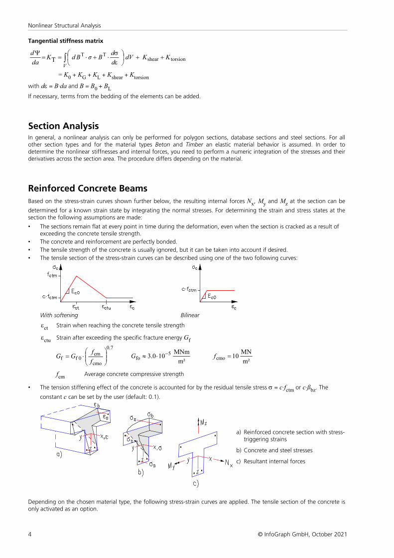
• The tensile section of the stress-strain curves can be described using one of the two following curves:

With softening Bilinear

ect Strain when reaching the concrete tensile strength

ectu Strain after exceeding the specific fracture energy Gf

7.0

cmo

cm0ff ÷

÷ø

öççè

æ×=

f

fGG

m²

MNm100.3 5

fo-×»G

m²

MN10cmo =f

fcm Average concrete compressive strength

• The tension stiffening effect of the concrete is accounted for by the residual tensile stress s = c·fctm or c·ßbz. The

constant c can be set by the user (default: 0.1).

a) Reinforced concrete section with stress-triggering strains

b) Concrete and steel stresses

c) Resultant internal forces

Depending on the chosen material type, the following stress-strain curves are applied. The tensile section of the concrete isonly activated as an option.

5

Basics


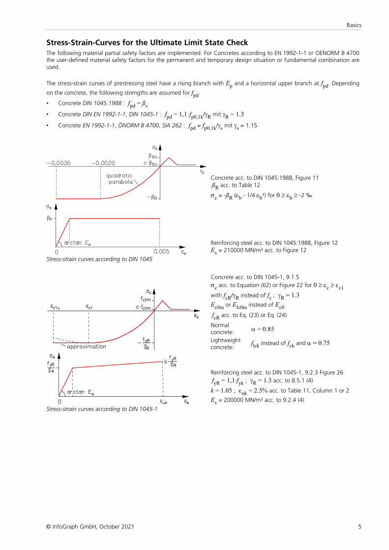
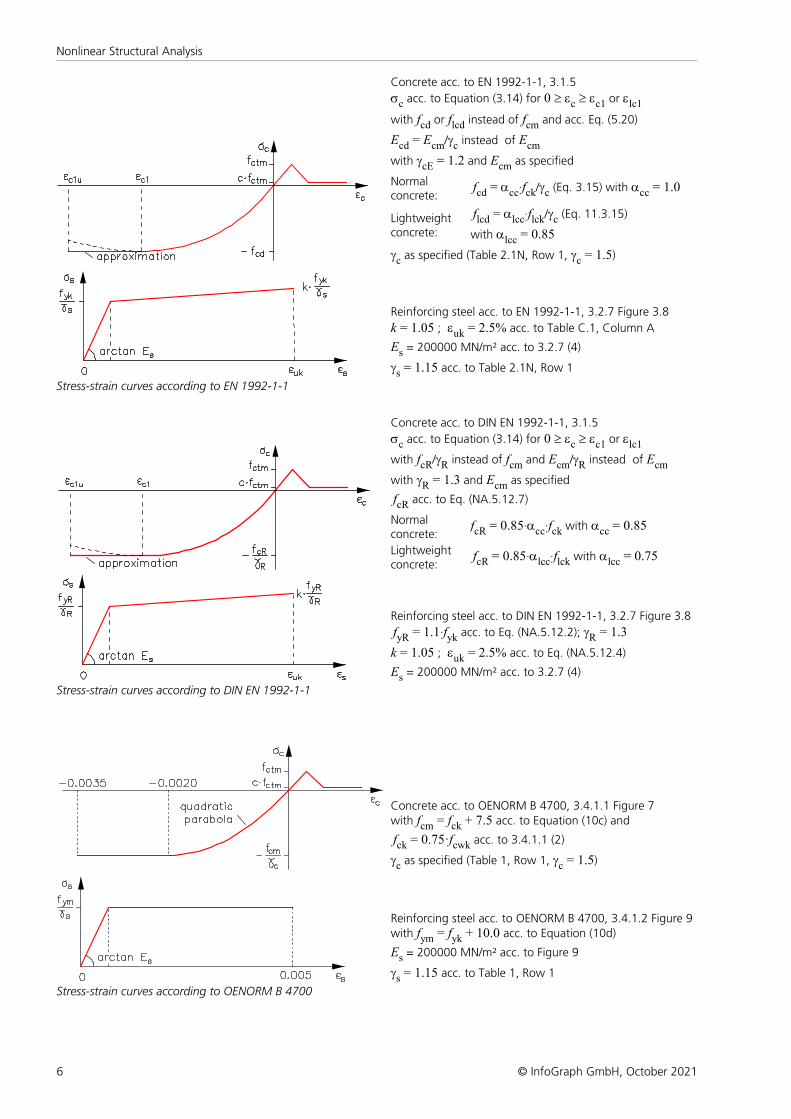
Stress-Strain-Curves for the Ultimate Limit State Check

The following material partial safety factors are implemented. For Concretes according to EN 1992-1-1 or OENORM B 4700the user-defined material safety factors for the permanent and temporary design situation or fundamental combination areused.

The stress-strain curves of prestressing steel have a rising branch with Ep and a horizontal upper branch at fpd. Depending

on the concrete, the following strengths are assumed for fpd.

• Concrete DIN 1045:1988 : fpd = ßs

• Concrete DIN EN 1992-1-1, DIN 1045-1 : fpd = 1,1·fp0,1k/gR mit gR = 1.3

• Concrete EN 1992-1-1, ÖNORM B 4700, SIA 262 : fpd = fp0,1k/gs mit gs = 1.15

Concrete acc. to DIN 1045:1988, Figure 11

ßR acc. to Table 12

sc = -ßR·(eb - 1/4·eb²) for 0 ³ eb ³ -2 ‰

Reinforcing steel acc. to DIN 1045:1988, Figure 12Es = 210000 MN/m² acc. to Figure 12

Stress-strain curves according to DIN 1045

Concrete acc. to DIN 1045-1, 9.1.5

sc acc. to Equation (62) or Figure 22 for 0 ³ ec ³ ec1

with fcR/gR instead of fc ; gR = 1.3

Ec0m or Elc0m instead of Ec0

fcR acc. to Eq. (23) or Eq. (24)

Normalconcrete:

a = 0.85

Lightweightconcrete: flck instead of fck and a = 0.75

Reinforcing steel acc. to DIN 1045-1, 9.2.3 Figure 26

fyR = 1,1·fyk ; gR = 1.3 acc. to 8.5.1 (4)

k = 1.05 ; euk = 2.5% acc. to Table 11, Column 1 or 2

Es = 200000 MN/m² acc. to 9.2.4 (4)

Stress-strain curves according to DIN 1045-1

6



Concrete acc. to EN 1992-1-1, 3.1.5

sc acc. to Equation (3.14) for 0 ³ ec ³ ec1 or elc1

with fcd or flcd instead of fcm and acc. Eq. (5.20)

Ecd = Ecm/gc instead of Ecm

with gcE = 1.2 and Ecm as specified

Normalconcrete: fcd = acc·fck/gc (Eq. 3.15) with acc = 1.0

Lightweightconcrete:

flcd = alcc·flck/gc (Eq. 11.3.15)

with alcc = 0.85

gc as specified (Table 2.1N, Row 1, gc = 1.5)

Reinforcing steel acc. to EN 1992-1-1, 3.2.7 Figure 3.8

k = 1.05 ; euk = 2.5% acc. to Table C.1, Column A

Es = 200000 MN/m² acc. to 3.2.7 (4)

gs = 1.15 acc. to Table 2.1N, Row 1

Stress-strain curves according to EN 1992-1-1

Concrete acc. to DIN EN 1992-1-1, 3.1.5


with fcR/gR instead of fcm and Ecm/gR instead of Ecm

with gR = 1.3 and Ecm as specified

fcR acc. to Eq. (NA.5.12.7)

Normalconcrete:

fcR = 0.85·acc·fck with acc = 0.85

Lightweightconcrete: fcR = 0.85·alcc·flck with alcc = 0.75

Reinforcing steel acc. to DIN EN 1992-1-1, 3.2.7 Figure 3.8

fyR = 1.1·fyk acc. to Eq. (NA.5.12.2); gR = 1.3

k = 1.05 ; euk = 2.5% acc. to Eq. (NA.5.12.4)

Es = 200000 MN/m² acc. to 3.2.7 (4)

Stress-strain curves according to DIN EN 1992-1-1

Concrete acc. to OENORM B 4700, 3.4.1.1 Figure 7with fcm = fck + 7.5 acc. to Equation (10c) and

fck = 0.75·fcwk acc. to 3.4.1.1 (2)

gc as specified (Table 1, Row 1, gc = 1.5)

Reinforcing steel acc. to OENORM B 4700, 3.4.1.2 Figure 9with fym = fyk + 10.0 acc. to Equation (10d)

Es = 200000 MN/m² acc. to Figure 9

gs = 1.15 acc. to Table 1, Row 1

Stress-strain curves according to OENORM B 4700

7

Basics


Concrete acc. to SIA 262, 4.2.1.6 and Figure 12

sc acc. to Equation (28) for 0 ³ ec ³ -2 ‰ with

fcd acc. to Eq. (2) and Eq. (26); gc = 1.5 acc. to 2.3.2.6

Ecd = Ecm / gcE acc. to Eq. (33)

Ecm acc. to Eq. (10) and Eq. (11)

gcE = 1.2 acc. to 4.2.1.17

Reinforcing steel acc. to SIA 262, 4.2.2.2, Figure 16

with fsd = fsk/gs acc. to Eq. (4); gs = 1.15 acc. to 2.3.2.6

ks = 1.05 and euk = 2 % acc. to Table 9, Column A


Stress-strain curves according to SIA 262

Stress-Strain-Curves for the Serviceability Check

The serviceability check is based on the average strengths of the materials. The partial safety factors are assumed to be 1.0.The stress-strain curves of prestressing steel have a rising branch with Ep and a horizontal upper branch at fp0,1k or ßs.

Concrete with linear stiffness in the compression zonewithout failure limit

Reinforcing steel acc. to DIN 1045:1988, Figure 12Es = 210000 MN/m² acc. to 6.2.1

Stress-strain curves according to DIN 1045

Concrete acc. to DIN 1045-1, 9.1.5

sc acc. to Equation (62) or Figure 22 for 0 ³ ec ³ ec1

with fcm or flcm instead of fc and Ec0m or Elc0m instead of Ec0

Reinforcing steel acc. to DIN 1045-1, 9.2.3 Figure 26

k = 1.05 ; euk = 2.5% acc. to Table 11, Column 1 or 2

Es = 200.000 MN/m² acc. to 9.2.4 (4)

Stress-strain curves according to DIN 1045-1

8



Concrete acc. to EN 1992-1-1, 3.1.5


with fcm acc. to Table 3.1 or flcm acc. to Table 11.3.1

and Ecm or Elcm as specified

Reinforcing steel acc. to EN 1992-1-1, 3.2.7 Figure 3.8

k = 1.05 ; euk = 2.5% acc. to Table C.1, Column A

Es = 200000 MN/m² acc. to 3.2.7 (4)

Stress-strain curves according to EN 1992-1-1

Concrete acc. to DIN EN 1992-1-1, 3.1.5


with fcm acc. to Table 3.1 or flcm acc. to Table 11.3.1

and Ecm or Elcm as specified

Reinforcing steel acc. to DIN EN 1992-1-1, 3.2.7 Figure 3.8

k = 1.05 ; euk = 2.5%

Es = 200000 MN/m²

Stress-strain curves according to DIN EN 1992-1-1

Concrete acc. to OENORM B 4700, 3.4.1.1 Figure 7with fcm = fck + 7.5 acc. to Equation (10c) and

fck = 0.75·fcwk acc. to 3.4.1.1 (2)

Reinforcing steel acc. to OENORM B 4700, 3.4.1.2 Figure 9with fym = fyk + 10.0 acc. to Equation (10d)


Stress-strain curves according to OENORM B 4700

9

Basics


Concrete acc. to SIA 262, 4.2.1.6 and Figure 12

sc acc. to Equation (28) for 0 ³ ec ³ -2 ‰ with

fcm = fck + 8 acc. to Eq. (6) instead of fcd

Ecm acc. to Eq. (10) and Eq. (11) instead of Ecd

Reinforcing steel acc. to SIA 262, 4.2.2.2, Figure 16with fsk instead of fsd

ks = 1.05 and euk = 2 % acc. to Table 9, Column A


Stress-strain curves according to SIA 262

Torsional Stiffness

When calculating the torsional stiffness of the section, it is assumed that it decreases at the same rate as the bendingstiffness.

÷÷

ø

ö

çç

è

æ+××=

Iz,

IIz,

Iy,

IIy,Ix,IIx,

2

1

EI

EI

EI

EIGIGI

The opposite case, meaning a reduction of the stiffnesses as a result of torsional load, cannot be analyzed. The physicalnonlinear analysis of a purely torsional load is also not possible for reinforced concrete.

Check of the Limit Strains (Ultimat Limit State Check)After completion of the equilibrium iteration the permissible limit strains for concrete and reinforcing steel are checked inthe case of frameworks (RSW, ESW) if the Newton analysis method is used. If the permissible values are exceeded thereinforcement will be increased or the load-bearing capacity will be reduced.

Automatic Reinforcement Increase (Ultimate Limit State Check)

If requested an automatic increase of reinforcement can be made for frameworks (RSW, ESW) with the Newton analysismethod to reach the full load-bearing capacity. Initially based on the desired start reinforcement the reachable load level isdetermined. If the reached load-bearing capacity is lower then 100%, the reinforcement will be increased and the iterationstarts again. If no load-bearing capacity exists because of insufficient start reinforcement a base reinforcement can bespecified within the reinforcing steel definition and the design can be performed again.

10



Concrete Creep

The consideration of concrete creep in nonlinear analysis is realized by modifying the underlying stress-strain curves. These

are scaled in strain-direction with the factor (1+j). Also the corresponding limit strains are multiplied by (1+j). Thefollowing figure shows the qualitative approach.

The described procedure postulates that the creep-generating stresses remain constant during the entire creep-period. Dueto stress redistributions, for example to the reinforcement, this can not be guaranteed. Therefore an insignificantoverestimation of the creep-deformations can occur.

Stress relaxation during a constant strain state can also be modelled by the described procedure. It leads, however, to anoverestimation of the remaining stresses due to the non-linear stress-strain curves.

The nonlinear concrete creep can be activated in the 'Load group' dialog.

This analysis approach applies analogous for area elements.

The plausibility of the achievable calculation results as well as the mode of action of different approaches for the concretetensile strength and the tension stiffening are demonstrated by two examples in the 'Crosscheck of Two Short-Term Tests'section.

Steel BeamsThe section geometry is determined by the polygon boundary. In order to perform the section analysis, the programinternally generates a mesh. The implemented algorithm delivers all section properties, stresses and internal forces on thebasis of the quasi-harmonic differential equation and others.

Stahlquerschnitt mit interner Vernetzung

The shear load is described by the following boundary value problem:

033

0

0

dR,2

xz2

xy2

x

xn

2

2

2

2

=s-t+t+s

=t

=¶

j¶+

¶

j¶

zy (Differential equation)

(Boundary condition)

(Yield criterion)

The differential equation holds equally for Qy, Qz and Mx. Depending on the load, the boundary condition delivers different

boundary values of the solution function j. The solution is arrived at by integral representation of the boundary valueproblem and discretization through finite differential equation elements. The internal forces are determined by numericalintegration of the stresses across the section under consideration of the Huber-von Mises yield criterion. The interaction ofall internal forces can be considered.

At the ultimate limit state, the material safety factor gM is taken into account as follows:

• Construction steel according to DIN 18800 and the general material type Stahl:

The factor gM of the fundamental combination according to DIN 18800 is decisive.

• Construction steel according to EN 10025-2:

In accordance with EN 1993-1-1, Chapter 6.1 (1), gM is assumed to be gM0 = 1.0.

The serviceability check is generally calculated with a material safety factor of gM = 1.0.

11

Basics


On the basis of DIN 18800, the interaction between normal and shear stresses is considered only when one of the followingthree conditions is met:

Qy ³ 0.25·Qpl,y,d

Qz ³ 0.33·Qpl,z,d

Mx ³ 0.20·Mpl,x,d

Limiting the bending moments Mpl,y,d and Mpl,z,d according to DIN 18800 to 1.25 times the corresponding elastic limit

moment does not occur.

Stability failure due to cross-section buckling or lateral torsional buckling is not taken into account.

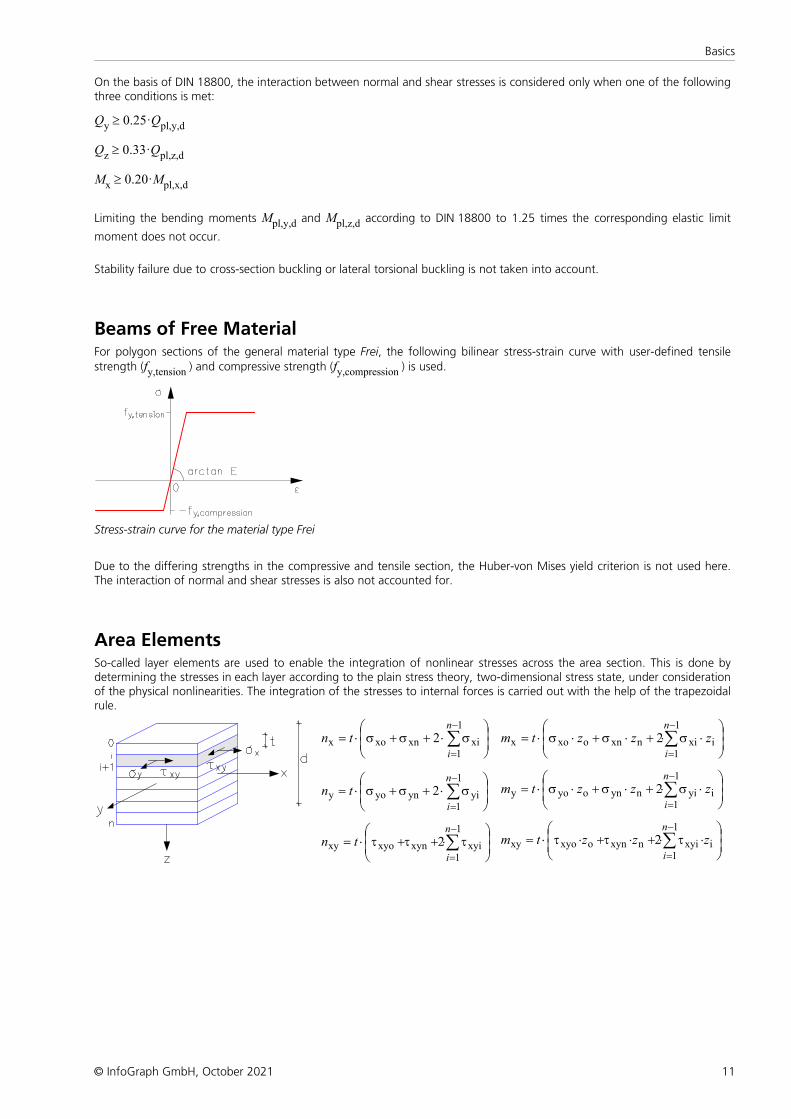
Beams of Free MaterialFor polygon sections of the general material type Frei, the following bilinear stress-strain curve with user-defined tensilestrength (fy,tension ) and compressive strength (fy,compression ) is used.

Stress-strain curve for the material type Frei

Due to the differing strengths in the compressive and tensile section, the Huber-von Mises yield criterion is not used here.The interaction of normal and shear stresses is also not accounted for.

Area ElementsSo-called layer elements are used to enable the integration of nonlinear stresses across the area section. This is done bydetermining the stresses in each layer according to the plain stress theory, two-dimensional stress state, under considerationof the physical nonlinearities. The integration of the stresses to internal forces is carried out with the help of the trapezoidalrule.

÷÷

ø

ö

çç

è

æs×+s+s×= å

-

=

1

1xixnxox 2

n

i

tn

÷÷

ø

ö

çç

è

æs×+s+s×= å

-

=

1

1yiynyoy 2

n

i

tn

÷÷

ø

ö

çç

è

æt×+t+t×= å

-

=

1

1xyixynxyoxy 2

n

i

tn

÷÷

ø

ö

çç

è

æ×s×+×s+×s×= å

-

=

1

1ixinxnoxox 2

n

i

zzztm

÷÷

ø

ö

çç

è

æ×s×+×s+×s×= å

-

=

1

1iyinynoyoy 2

n

i

zzztm

÷÷

ø

ö

çç

è

æ×t×+×t+×t×= å

-

=

1

1ixyinxynoxyoxy 2

n

i

zzztm

12



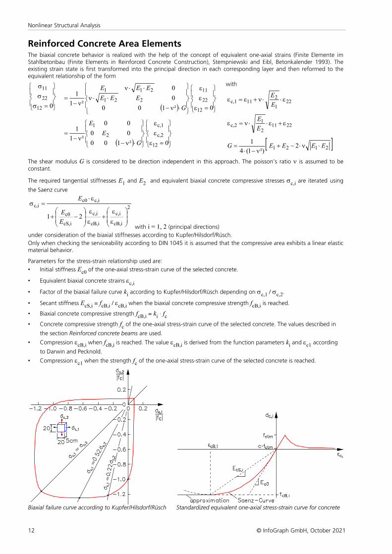
Reinforced Concrete Area ElementsThe biaxial concrete behavior is realized with the help of the concept of equivalent one-axial strains (Finite Elemente imStahlbetonbau (Finite Elements in Reinforced Concrete Construction), Stempniewski and Eibl, Betonkalender 1993). Theexisting strain state is first transformed into the principal direction in each corresponding layer and then reformed to theequivalent relationship of the form

ïþ

ïý

ü

ïî

ïí

ì

=s

s

s

012

22

11

( ) ïþ

ïý

ü

ïî

ïí

ì

=e

e

e

ïþ

ïý

ü

ïî

ïí

ì

×n-

××n

××n

n-=

0²100

0

0

²1

1

12

22

11

221

211

G

EEE

EEE

( ) ïþ

ïý

ü

ïî

ïí

ì

=e

e

e

ïþ

ïý

ü

ïî

ïí

ì

×n-n-

=

0²100

00

00

²1

1

12

c,2

c,1

2

1

G

E

E

with

221

211c,1 e××n+e=e

E

E

22112

1c,2 e+e××n=e

E

E

[ ]2121 2²)1(4

1EEEEG ×n×-+

n-×=

The shear modulus G is considered to be direction independent in this approach. The poisson's ratio n is assumed to beconstant.

The required tangential stiffnesses E1 and E2 and equivalent biaxial concrete compressive stresses sc,i are iterated using

the Saenz curve

2

cB,i

c,i

cB,i

c,i

cS,i

c0

c,ic0c,i

21÷÷

ø

ö

çç

è

æ

e

e+

e

e

÷÷

ø

ö

çç

è

æ-+

e×=s

E

E

E

with i = 1, 2 (principal directions)

under consideration of the biaxial stiffnesses according to Kupfer/Hilsdorf/Rüsch.

Only when checking the serviceability according to DIN 1045 it is assumed that the compressive area exhibits a linear elasticmaterial behavior.

Parameters for the stress-strain relationship used are:

• Initial stiffness Ec0 of the one-axial stress-strain curve of the selected concrete.

• Equivalent biaxial concrete strains ec,i

• Factor of the biaxial failure curve ki according to Kupfer/Hilsdorf/Rüsch depending on sc,1 / sc,2.

• Secant stiffness EcS,i = fcB,i / ecB,i when the biaxial concrete compressive strength fcB,i is reached.

• Biaxial concrete compressive strength fcB,i = ki · fc• Concrete compressive strength fc of the one-axial stress-strain curve of the selected concrete. The values described in

the section Reinforced concrete beams are used.

• Compression ecB,i when fcB,i is reached. The value ecB,i is derived from the function parameters ki and ec1 according

to Darwin and Pecknold.

• Compression ec1 when the strength fc of the one-axial stress-strain curve of the selected concrete is reached.

Biaxial failure curve according to Kupfer/Hilsdorf/Rüsch Standardized equivalent one-axial stress-strain curve for concrete

13

Basics


Stress-strain curve for the serviceability check according to DIN 1045

The consideration of the concrete creep occurs analog to the procedure for beams through modification of the underlyingstress-strain curves and can be activated in the 'Load group' dialog.

Interaction with the shear stresses from the lateral forces is not considered here. During the specification of thecrack direction the so-called 'rotating crack model' is assumed, meaning that the crack direction can change during thenonlinear iteration as a function of the strain state. Conversely, a fixed crack direction after the initial crack formation canlead to an overestimation of the load-bearing capacity.

The Finite Element module currently does not check the limit strain nor does it automatically increasereinforcement to improve the load-bearing capacity due to the significant numerical complexity.

For clarification of the implemented stress-strain relationships for concrete, the curves measured in the biaxial test accordingto Kupfer/Hilsdorf/Rüsch are compared with those calculated using the approach described above.

Biaxial test according to Kupfer/Hilsdorf/Rüsch

Calculation results for C25/30; fcm = 25 + 8 = 33 MN/m²

14



The existing reinforcing steel is modeled as a 'blurred' orthogonal reinforcement mesh. The corresponding strain state istransformed into the reinforcement directions (p, q) of the respective reinforcing steel layer. The stress-strain curve of theselected reinforced concrete standard is used to determine the stress.

Area Elements of Steel and Free MaterialFor area elements made of steel the Huber v.Mises yield criterion is used. The material safety factor specified in the sectionSteel beams apply accordingly. For area elements of the material type Frei, the Raghava or the Rankine yield criterion can bechosen.

F = J2 - 1/3 × fyc × fyt + ( fyc - fyt ) × sm = 0

with

sm = 1/3 ( sx + sy + sz )

J2 = 1/2 ( s²x + s²y + s²z ) + t²xy + t²yz + t²zx

sx = sx - sm

sy = sy - sm

sz = sz - sm

Starting from the strain state, a layer is iterated on the yield surface with the help of a 'backward Euler return' that, inconjunction with the Newton-Raphson method, ensures quadratic convergence. (Non-linear Finite Element Analysis of Solidsand Structures, M.A. Crisfield, Publisher John Wiley & Sons).

The yield surface mentioned above is illustrated below for the 2D stress state, as used for layer elements, for the principal

stresses s1 and s2 as well as for the components sx, sy and txy.

In this example fyc = 20 MN/m² and fyt = 2 MN/m².

0-10

-20-30

-10

-5

0

5

10

-10

-5

0

5

10

sy

txy

sx

-20

= 0t

sx

xy

s

2

y

-20

s x=s y

Yield surface for the 2D stress state according to Raghava

15

Basics


Solid ElementsFor solid elements of steel or standardized type of concrete the Raghava yield criterion is used (see Area elements of steeland free material). For solid elements of the material type Frei the yield criterion can be chosen in the material propertydialog. All other material types are assumed to be elastic. The compressive strength fyc of the standardized concrete types is

fck in the serviceability limit state and fcd in the ultimate limit state. The concrete tensile strength is c·fctm if the analysis

settings with softening or bilinear are selected or zero in all other cases. At the moment a softening of the material in thetensile area is not supported for solid elements. The failure criteria of concrete are not represented correctly with theyield criteria pictured below.

2

1s2

-20

-20

= 0s3

s

s 1=s 2

Yield surface according to Raghava for principal stresses s1, s2 and s3 with fyc = 20 MN/m² and fyt = 2 MN/m²

For materials with identical tensile and compressive strength the yield criterion of Raghava is equivalent to the Huber-v.Mises yield criterion.

-235

235

-235

= 0s3 235

s2

s1

2s=

1s

Yield surface according to Raghava for principal stresses s1, s2 and s3 with fyc = 235 MN/m² and fyt = 235 MN/m²

2

1s2

-20

-20

= 0s3

s

s 1=s 2

Yield surface according to Rankine for principal stresses s1, s2 and s3 with fyc = 20 MN/m² and fyt = 2 MN/m²

16



Prestressed StructuresPrestressing is often considered only as an external load. Therefore, no stress redistributions between concrete andprestressing steel can be taken into account. But the consideration of this redistributions is also possible. For this purpose,the tendons are included in the element stiffness matrices during the calculation. This method is implemented for allelement types. The internal forces (normal forces, bending moments, lateral forces) given by the program always correspondto the concrete section with its reinforcing steel layers. When analyzing composite elements, these alone are not inequilibrium with the external forces since the tendon group forces must be applied while taking into account their spatialorientation. Because the program assumes that a tendon runs straight between the entry and exit points of an element, anadequate FE mesh is especially important for beam elements. Area and solid models, on the other hand, generally exhibit asufficiently fine discretization.

The stress-strain curves of prestressing steel in the serviceability limit state have a rising branch with Ep and a horizontal

upper branch at fp0,1k or ßs. In the ultimate limit state the upper branch is at fpd. Depending on the concrete, the following

strengths are assumed for fpd.

• Concrete DIN 1045:1988 fpd = ßs

• Concrete DIN EN 1992-1-1, DIN 1045-1 fpd = 1,1·fp0,1k/gR mit gR = 1.3

• Concrete EN 1992-1-1, ÖNORM B 4700, SIA 262 fpd = fp0,1k/gs mit gs = 1.15

Notes on Convergence BehaviorThe implemented analysis methods (Newton method, arc length method) with tangential stiffness matrix result in a stableconvergence behavior given a consistent relationship between the stress-strain relation and its derivative. As previouslymentioned, this is especially true of bilinear materials. Reinforced concrete, however, typically displays a poor convergencedue to its more complex material properties. This is caused by crack formation, not continuously differentiable stress-strainrelationships, two-component materials, etc.

Especially for checks of the serviceability and determination of the tensile stiffness with softening, markedly worseconvergence can result due to the negative tangential stiffness in the softening area. If this results in a singular globalstiffness matrix, it is possible to assume a bilinear function in the tensile section or to perform a calculation without tensilestrength.

17

Analysis Settings


Analysis SettingsThe following settings are made on the Ultimate Limit state and the Serviceability tabs in the Settings for the nonlinearanalysis of the menu item Analysis - Settings.

With the nonlinear system analysis, load cases are calculated under consideration of physical and geometrical nonlinearities,whereby the latter only becomes active if the second- or third order theory is activated in the load case. The load bearingcapacity and serviceability check as well as the stability check for fire differ according to the load case that is to be checked,the material safety, the different stress-strain-curves and the consideration of the concrete tensile strength.

Consider the following load cases

The load cases from the left list box are calculated.

Start reinforcement

The nonlinear system analysis is carried out on reinforced concrete sections based on the reinforcement selected here. Thisresults from a reinforced concrete design carried out in advance. The starting reinforcement Null corresponds to the basereinforcement of the reinforcing steel layers. When performing a check for fire scenarios, special conditions apply asexplained in the Structural Analysis for Fire Scenarios chapter.

Automatic reinforcement increase frame

For the ultimate limit state check of pure frameworks a reinforcement increase is carried out for reinforced concrete sectionsto achieve the required load-bearing safety.

Concrete tensile strength; Factor c

This option defines the behavior in the tensile zone for the nonlinear internal forces calculation for all reinforced concretesections. By default the ultimate limit state check is performed without considering the concrete tensile strength.

With softening (beams) With softening (area elements) Bilinear

Layers per area element

Number of integration levels of an area element. Members subject to bending should be calculated with 10 layers. Structuremostly subject to normal forces can be adequately analyzed with 2 layers.

Consider tendons

The tendons are considered in the calculation of the element stiffness matrices.

18



Constant stiffness

The iteration is done with a constant stiffness matrix. If the switch is not set, then a tangential stiffness matrix is used.

Analysis method

The following methods are available:

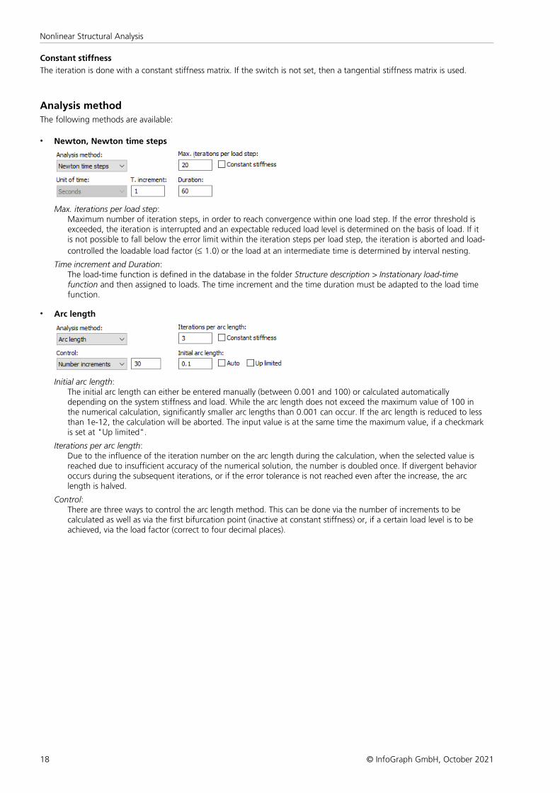
• Newton, Newton time steps

Max. iterations per load step:Maximum number of iteration steps, in order to reach convergence within one load step. If the error threshold isexceeded, the iteration is interrupted and an expectable reduced load level is determined on the basis of load. If itis not possible to fall below the error limit within the iteration steps per load step, the iteration is aborted and load-

controlled the loadable load factor (£ 1.0) or the load at an intermediate time is determined by interval nesting.

Time increment and Duration:The load-time function is defined in the database in the folder Structure description > Instationary load-timefunction and then assigned to loads. The time increment and the time duration must be adapted to the load timefunction.

• Arc length

Initial arc length:The initial arc length can either be entered manually (between 0.001 and 100) or calculated automaticallydepending on the system stiffness and load. While the arc length does not exceed the maximum value of 100 inthe numerical calculation, significantly smaller arc lengths than 0.001 can occur. If the arc length is reduced to lessthan 1e-12, the calculation will be aborted. The input value is at the same time the maximum value, if a checkmarkis set at "Up limited".

Iterations per arc length:Due to the influence of the iteration number on the arc length during the calculation, when the selected value isreached due to insufficient accuracy of the numerical solution, the number is doubled once. If divergent behavioroccurs during the subsequent iterations, or if the error tolerance is not reached even after the increase, the arclength is halved.

Control:There are three ways to control the arc length method. This can be done via the number of increments to becalculated as well as via the first bifurcation point (inactive at constant stiffness) or, if a certain load level is to beachieved, via the load factor (correct to four decimal places).

19

Examples


Examples

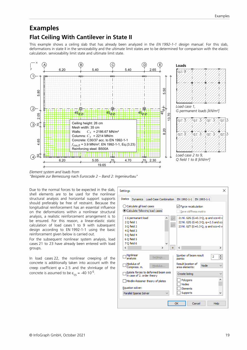
Flat Ceiling With Cantilever in State IIThis example shows a ceiling slab that has already been analyzed in the EN 1992-1-1 design manual. For this slab,deformations in state II in the serviceability and the ultimate limit states are to be determined for comparison with the elasticcalculation. serviceability limit state and ultimate limit state.

5.405.406.20 2.65

8.2

0

13.7

0

5.5

019.65

2.3070705.056.20 4.70

50

2.0

57

04

.65

5.8

0

1

2

4

3

A B C D E

45 45 45 45

z

z = 2186.67 MN/m²

= 2214 MN/mCC

Columns:

Concrete: C30/37 acc. to EN 1992-1-1

Reinforcing steel: B500A

Mesh width: 35 cm

Ceiling height: 26 cm

Walls:

fctm,fl = 3.9 MN/m², EN 1992-1-1, Eq.(3.23)

Element system and loads from"Beispiele zur Bemessung nach Eurocode 2 – Band 2: Ingenieurbau"

Loads

Load case 1, G permanent loads [kN/m²]

Load case 2 to 9, Q field 1 to 8 [kN/m²]

Due to the normal forces to be expected in the slab,shell elements are to be used for the nonlinearstructural analysis and horizontal support supportsshould preferably be free of restraint. Because thelongitudinal reinforcement has an essential influenceon the deformations within a nonlinear structuralanalysis, a realistic reinforcement arrangement is tobe ensured. For this reason, a linear-elastic staticcalculation of load cases 1 to 9 with subsequentdesign according to EN 1992-1-1 using the basicreinforcement given below is carried out.

For the subsequent nonlinear system analysis, loadcases 21 to 23 have already been entered with loadgroups.

In load cases 22, the nonlinear creeping of theconcrete is additionally taken into account with the

creep coefficient j = 2.5 and the shrinkage of the

concrete is assumed to be ecs = -40·10-5.

20



Reinforcement for area elements

No. Lay. Qual. d1x d2x asx d1y d2y asy as Roll-[m] [m] [cm²/m] [m] [m] [cm²/m] fix ing

1 1 500M 0.045 5.670 0.035 5.650 Warm2 500M 0.035 7.850 0.025 5.030 Warm

2 1 500M 0.045 5.670 0.035 5.650 Warm2 500M 0.035 7.850 0.025 11.340 Warm

as Base reinforcement d1 Distance from the upper edge d2 Distance from the lower edge

The z axis of the element system points to the lower edge

Bending reinforcement from design of the permanent and temporary situation

Only in the area around the columns and the corners does a reinforcement increase result in the upper reinforcement layers,which approximately corresponds to the additional reinforcement provided in the literature example.

Additional reinforcement asx.1 [cm²/m]

0.01

2.00

4.00

6.00

8.00

10.00

15.00

Additional reinforcement asy.1 [cm²/m]

Analysis settingsAfter the elastic static calculation of load cases 1 to 9 and the subsequent design according to EN 1992-1-1, the nonlinearsystem analysis is selected in the static analysis settings and the following settings are made.

For the load cases (21 and 22) for serviceability,softening and a residual tensile strength of c·fctm,fl =

0.1·3.9 = 0.39 MN/m² are calculated in the tensilezone of the concrete.

Load case 23 for the ultimate limit state is calculatedwithout considering the concrete tensile strength.

In order to increase the accuracy of the calculation,the error threshold is set to 0.1 % in the loadgroups. Therefore, the number of maximumiterations per load level is increased to 500.

21

Examples


Deformations

The different deformation results are compared below. For better comparison all non-linearly calculated load cases,including the one in the GZT, are calculated with the load G+0.3·Q. In all cases a load factor of 1.0 can be achieved.

Load cases 21: Deformations uz [mm]

-5.00

0.00

5.00

10.00

15.00

20.00

25.00

30.00

35.00

40.00

Load cases 22: Deformations uz [mm]

In the following, the maximum calculated deformations in state II are compared with the results determined in state I (seeexample for EN 1992-1-1):

max uz [mm]

Load case Calculation Literature

(11) G+0.3·Q with elastic material behavior (state I) 10 10

(12) Creeping (j=2.5 by LC 11) with elastic material behavior (state I) 23 -

(13) Total (load case 11 + load case 12) (state I) 33 -

21 Nl. GZG (G+0.3·Q, j and ecs=0 with softening) 18 20

22 Nl. GZG (G+0.3·Q, j=2.5 and ecs=-40·10-5 with softening) 43 40

23 Nl. GZT (G+0.3·Q, j and ecs=0 without concrete tensile strength) 56 -

Concrete stresses

Load case 22: Concrete stresses [MN/m²] in y-direction at the bottom

22



Crosscheck of Two Short-Term TestsIn the following section two simple structures made of reinforced concrete (taken from Krätzig/Meschke 2001) are analyzed.The goal is to demonstrate the plausibility of the achieved calculation results as well as the mode of action of differentapproaches for determining concrete tensile strength and tension stiffening.

Reinforced Concrete SlabThe system described below was analyzed experimentally by Jofriet & McNeice in 1971. For the crosscheck a system with20x20 shell elements was used as illustrated below.

Material:

fc = 37.92 [MPa]

Ec= 28613 [MPa]

vc= 0.15

ft = 2.91 [MPa]

Es= 201300 [MPa]

fy = 345.4 [MPa]

Element system with supports, load and the specified material parameters.

The load-displacement curve determined in the test for the slab middle is contrasted with the results of the static calculationin the following diagram. For the SLS the calculation method "Newton time steps" was chosen with 60 time increments andan error threshold of 0.1%. The material parameters were set according to the specifications of the authors. The materialtype ÖNBeton with the following material parameters was used for this:

fcwk = (fc - 7.5)/0.75 = 40.56 [MPa] fctm = ft = 2.91 [MPa]

0

2

4

6

8

10

12

14

0 1 2 3 4 5 6 7 8 9 10

Central deflection uz [mm]

Load P [kN]

Experiment (Jofriet & McNeice 1971)

with softening in the concrete tensile area; c=0.3

with softening in the concrete tensile area; c=0.2

with bilinear concrete tensile strength; c=0.2

without concrete tensile strength

Load-displacement curves from the crosscheck and experiment (Jofriet/McNeice)

In order to demonstrate the mode of action of the methods implemented in the program for the concrete tensile stresses,four variants were calculated. The curve accounting for the concrete tensile strength with softening (c=0.3) exhibits theclosest agreement with the test results. The behavior at the beginning of crack formation as well as close to load-bearingcapacity display a large level of agreement.

The curve for the bilinear behavior in the concrete tensile area was calculated with the value (c=0.2). The stiffness of theslab is thus, as expected, underestimated at the beginning of crack formation. The load-bearing safety is, however, hardlyinfluenced by this. This means that the calculation is on the safe side.

The curve for the 'naked state II' is for the most part determined by the characteristic curve of the reinforcing steel and thushas exhibits nearly linear behavior in the area under examination. Here as well a comparable load-bearing safety results interms of the plasticity theory; however, with significantly larger deformations.

23

Examples


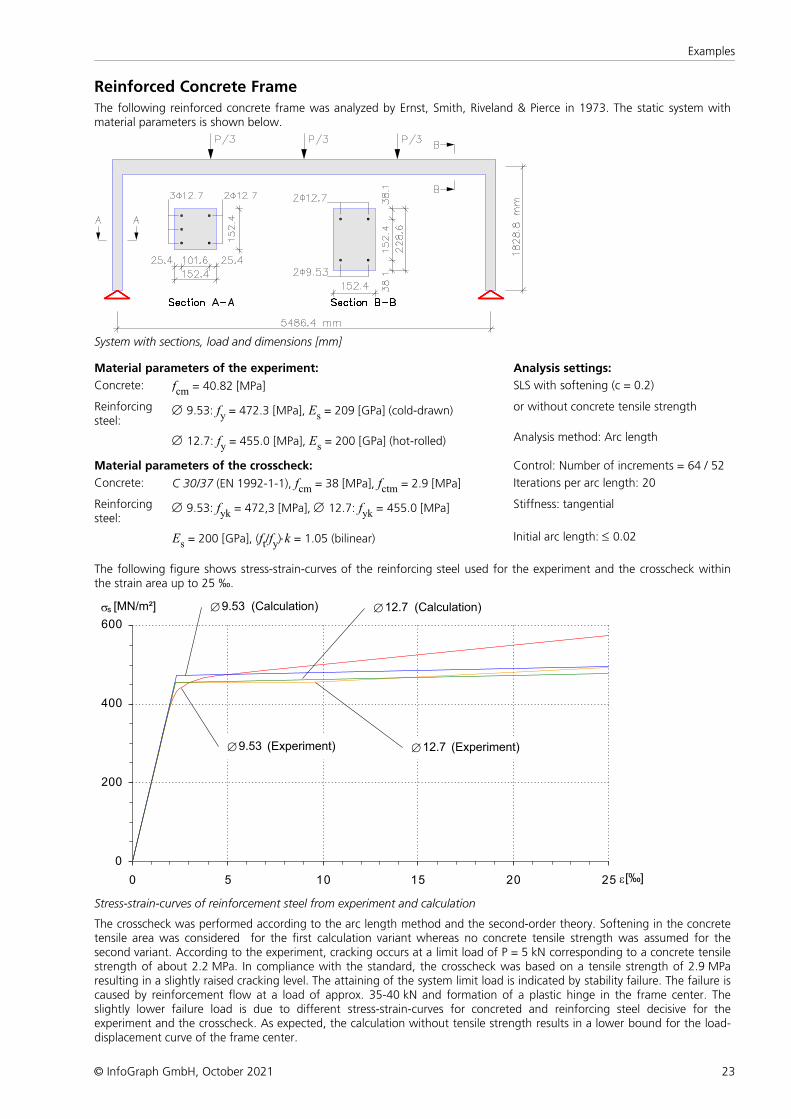
Reinforced Concrete Frame

The following reinforced concrete frame was analyzed by Ernst, Smith, Riveland & Pierce in 1973. The static system withmaterial parameters is shown below.

System with sections, load and dimensions [mm]

Material parameters of the experiment: Analysis settings:

Concrete: fcm = 40.82 [MPa] SLS with softening (c = 0.2)

Reinforcingsteel:

Æ 9.53: fy = 472.3 [MPa], Es = 209 [GPa] (cold-drawn) or without concrete tensile strength

Æ 12.7: fy = 455.0 [MPa], Es = 200 [GPa] (hot-rolled) Analysis method: Arc length

Material parameters of the crosscheck: Control: Number of increments = 64 / 52

Concrete: C 30/37 (EN 1992-1-1), fcm = 38 [MPa], fctm = 2.9 [MPa] Iterations per arc length: 20

Reinforcingsteel:

Æ 9.53: fyk = 472,3 [MPa], Æ 12.7: fyk = 455.0 [MPa] Stiffness: tangential

Es = 200 [GPa], (ft/fy)×k = 1.05 (bilinear) Initial arc length: £ 0.02

The following figure shows stress-strain-curves of the reinforcing steel used for the experiment and the crosscheck withinthe strain area up to 25 ‰.

0

200

400

600

0 5 10 15 20 25 e [‰]

ss [MN/m²] Æ9.53 (Calculation)

Æ9.53 (Experiment)

Æ12.7 (Calculation)

Æ12.7 (Experiment)

Stress-strain-curves of reinforcement steel from experiment and calculation

The crosscheck was performed according to the arc length method and the second-order theory. Softening in the concretetensile area was considered for the first calculation variant whereas no concrete tensile strength was assumed for thesecond variant. According to the experiment, cracking occurs at a limit load of P = 5 kN corresponding to a concrete tensilestrength of about 2.2 MPa. In compliance with the standard, the crosscheck was based on a tensile strength of 2.9 MParesulting in a slightly raised cracking level. The attaining of the system limit load is indicated by stability failure. The failure iscaused by reinforcement flow at a load of approx. 35-40 kN and formation of a plastic hinge in the frame center. Theslightly lower failure load is due to different stress-strain-curves for concreted and reinforcing steel decisive for theexperiment and the crosscheck. As expected, the calculation without tensile strength results in a lower bound for the load-displacement curve of the frame center.

24



0

10

20

30

40

0 20 40 60 80 100 120 140

Load P [kN]

Deflection w [mm]

Calculation with softening in the concrete tensile area; c=0.2

Calculation without concrete tensile strength

Experiment (Ernst et al. 1973)

P/3 P/3 P/3

w

Load-displacement curves from the crosscheck and experiment (Ernst et al. 1973)

Prestressed Concrete StructureIn this example an experiment of a prestressed two-span beam DLT1 with subsequent bond has been recalculated, whichhas been carried out at the TU Dortmund as part of a research project of the BASt (Maurer et al., 2015). The dimensions ofthe test beam are shown below. The structure has a T-beam cross section with a constant height of 80 cm. Also the flangedimensions are constant about the length of the beam with b/h = 80/15 cm. The web thickness within the fields and at theinner support is 30 cm. In the area of the end supports the web thickness increase to 60 cm. For the calculation model ashell structure ( mesh width 5 cm) made of concrete ( C35/45 acc. to DIN 1045-1) with beam elements made of steel for thelongitudinal and shear reinforcement has been chosen. The assumed strengths of the steel layers are given below. For theconcrete behavior in the tension zone softening with a residual tensile strength of 0.1·fctm has been assumed. The tendon

group is automatically implemented in the element stiffness matrices of the area elements by the program during the loadcase calculation.

3D view of the calculation model

d=60d=30

d=60d=30

8.4°d=80 d=80

60 50

6.00 6.00

12.00

2.25 3.50 3.50 2.25

50 60

8.4°

65

15

View with system dimensions and depiction of the tendon group

37

.3

62

.963

.463

.462

.961

.659

.356

.452

.848

.944

.640

.135

.831

.427

.423

.820

.918

.817

.316

.516

.516

.717

.117

.618

.619

.821

.323

.225

.728

.531

.333

.8

37

.3

61

.6

33

.831

.328

.525

.7

21

.319

.818

.617

.6

16

.716

.516

.517

.318

.820

.923

.827

.431

.435

.840

.144

.648

.952

.856

.459

.3

23

.2

17

.1

25 2557 x 20

Distance between center axis of the tendon group and the bottom edge of the beam

25

Examples


11.90

10

78.1

xv

[m]5.95

11

91.6

fp A mm²1400=

MN/m²= 199700E-Modul

p0.1k = 1666 MN/m²

1210.7

0.00

10

78.1

[kN

]

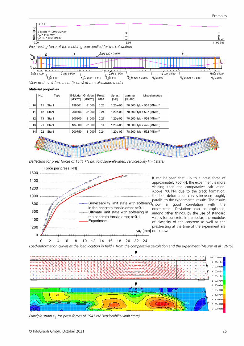
Prestressing force of the tendon group applied for the calculation

22 5 ø12/922 8 ø12/20 21 27 ø8/20

13 3 ø16 12 2 ø20 + 3 ø16 11 2 ø25 + 3 ø16

44

4 155

59

12 2 ø20 + 3 ø1613 3 ø1613 3 ø16 13 3 ø16

21 27 ø8/2022 5 ø12/9

12 2 ø20 + 3 ø16

View of the reinforcement (beams) of the calculation model

Material properties

No. Type E-Modu. G-Modu. Poiss. alpha.t gamma Miscellaneous[MN/m²] [MN/m²] ratio [1/K] [kN/m³]

10 11 Stahl 199501 81000 0.23 1.20e-05 78.500 fyk = 555 [MN/m²]

11 12 Stahl 200506 81000 0.24 1.20e-05 78.500 fyk = 567 [MN/m²]

12 13 Stahl 205200 81000 0.27 1.20e-05 78.500 fyk = 554 [MN/m²]

13 21 Stahl 184000 81000 0.14 1.20e-05 78.500 fyk = 475 [MN/m²]

14 22 Stahl 200750 81000 0.24 1.20e-05 78.500 fyk = 532 [MN/m²]

Deflection for press forces of 1541 kN (50 fold superelevated, serviceability limit state)

0

200

400

600

800

1000

1200

1400

1600

0 2 4 6 8 10 12 14 16 18 20 22 24

Duz [mm]

Serviceability limit state with softeningin the concrete tensile area; c=0.1Ultimate limit state with softening inthe concrete tensile area; c=0.1Experiment

Force per press [kN]

It can be seen that, up to a press force ofapproximately 700 kN, the experiment is moreyielding than the comparative calculation.Above 700 kN, due to the crack formation,the load deformation curves increase roughlyparallel to the experimental results. The resultsshow a good correlation with theexperiments. Deviations can be explained,among other things, by the use of standardvalues for concrete. In particular, the modulusof elasticity of the concrete as well as theprestressing at the time of the experiment arenot known.

Load-deformation curves at the load location in field 1 from the comparative calculation and the experiment (Maurer et al., 2015)

Principle strain e1 for press forces of 1541 kN (serviceability limit state)

26



Prestressing steel stresses sp [MN/m²] for press forces of 0 and 1541 kN (serviceability limit state)

Reinforcing steel stresses sv [MN/m²] for press forces of 1541 kN (serviceability limit state)

Horizontal concrete stresses sx [MN/m²] between the stirrups for press forces of 1541 kN (serviceability limit state)

Crack formation of the experiment for press forces of 800 kN (BASt Book B 120, Figure 70)

Strains eCrack when exceeding the tensile strength of concrete for press forces of 800 kN (ultimate limit state)

Crack formation of the experiment for press forces of 1541 kN (BASt Book B 120, Figure 73)

Strains eCrack when exceeding the tensile strength of concrete for press forces of 1541 kN (ultimate limit state)

27

Examples


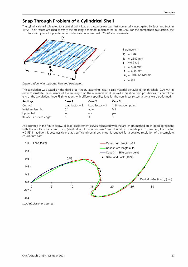
Snap Through Problem of a Cylindrical ShellThe cylindrical shell subjected to a central point load as shown below was first numerically investigated by Sabir and Lock in1972. Their results are used to verify the arc length method implemented in InfoCAD. For the comparison calculation, thestructure with jointed supports on two sides was discretized with 20x20 shell elements.

Parameters:

Pc = 1 kN

R = 2540 mm

Q = 0,2 rad

L = 508 mm

t = 6.35 mm

Es= 3102.64 MN/m²

v = 0.3Discretization with supports, load and parameters

The calculation was based on the third order theory assuming linear-elastic material behavior (Error threshold 0.01 %). Inorder to illustrate the influence of the arc length on the numerical result as well as to show two possibilities to control theend of the calculation, three FE simulations with different specifications for the non-linear system analysis were performed.

Settings: Case 1 Case 2 Case 3

Control: Load factor = 1 Load factor = 1 1. Bifurcation point

Initial arc length: 0.1 auto 0.1

Up limited: yes no yes

Iterations per arc length: 3 3 3

As illustrated in the figure below, all load-displacement curves calculated with the arc length method are in good agreementwith the results of Sabir and Lock. (identical result curve for case 1 and 3 until first branch point is reached, load factor= 0.53) In addition, it becomes clear that a sufficiently small arc length is required for a detailed resolution of the completeequilibrium path.

0.53

-0.4

-0.2

0.0

0.2

0.4

0.6

0.8

1.0

0 5 10 15 20 25 30

Central deflection uz [mm]

Load factor Case 1: Arc length 0.1

Case 2: Arc length auto

Case 3: 1. Bifurcation point

Sabir and Lock (1972)

£

Load-displacement curves

28



ReferencesBeispiele zur Bemessung nach Eurocode 2 – Band 2: Ingenieurbau.

Publisher: Deutscher Beton- und Bautechnik-Verein E.V., Ernst & Sohn Verlag, Berlin 2015.

Crisfield, M.A.Non-linear Finite Element Analysis of Solids and Structures.John Wiley & Sons, Ltd. New York 1991.

Darwin, D.; Pecknold, D.A.W.Inelastic Model for Cyclic Biaxial Loading of Reinforced Concrete.A Report on a Research Project Sponsored by The National Science Foundation, Research Grant GI 29934University of Illinois at Urbana-Champaign Urbana, Illinois 1974.

DIN EN 1992-1-1/NA:2013+A1:2015-12National Annex – Nationally determined parameters –Eurocode 2: Design of concrete structures – Part 1-1: General rules and rules for buildings.Publisher: DIN Deutsches Institut für Normung e.V., Beuth Verlag GmbH, Berlin 2015.

DIN 1045-1:2008-08 (New Edition)Concrete, reinforced and prestressed concrete structures – Part 1: Design and construction.Publisher: DIN Deutsches Institut für Normung e.V., Beuth Verlag GmbH, Berlin 2008.

DIN 1045, Edition July 1988Structural use of concrete – Design and construction.Publisher: DIN Deutsches Institut für Normung e.V., Beuth Verlag GmbH, Berlin 1988.

DIN 18800:2008-11Stahlbauten (Steel Structures) – Part 1 to Part 4.Publisher: DIN Deutsches Institut für Normung e.V., Beuth Verlag GmbH, Berlin 2008.

Duddeck, H.; Ahrens, H.Statik der Stabwerke (Statics of Frameworks), Betonkalender 1985. Ernst & Sohn Berlin 1985.

EN 1992-1-1:2004+A1:2014Eurocode 2: Design of concrete structures – Part 1-1: General rules and rules for buildings.Publisher: CEN European Committee for Standardization, Brussels. Beuth Verlag GmbH, Berlin 2014.

EN 1993-1-1:2005+A1:2014Eurocode 3: Design of steel structures – Part 1-1: General rules and rules for buildings.Publisher: CEN European Committee for Standardization, Brussels. Beuth Verlag GmbH, Berlin 2014.

EN 10025-2:2019-10Hot rolled products of structural steels – Part 2: Technical delivery conditions for non-alloy structural steels.Publisher: CEN European Committee for Standardization, Brussels. Beuth Verlag GmbH, Berlin 2019.

Ernst, G.C.; Smith, G.M.; Riveland, A.R.; Pierce, D.N.Basic reinforced concrete frame performance under vertical and lateral loads.ACI Material Journal 70(28), pp. 261-269. American Concrete Institute, Farmingten Hills 1973.

Hirschfeld, K.Baustatik Theorie und Beispiele (Structural Analysis Theory and Examples).Springer Verlag, Berlin 1969.

Jofriet, J.C.; McNeice, M.Finite element analysis of reinforced concrete slabs.Journal of the Structural Division (ASCE) 97(ST3), pp. 785-806. American Society of Civil Engineers, New York 1971.

Kindmann, R.Traglastermittlung ebener Stabwerke mit räumlicher Beanspruchung(Limit Load Determination of 2D Frameworks with 3D Loads).Institut für Konstruktiven Ingenieurbau, Ruhr-Universität Bochum, Mitteilung Nr. 813, Bochum 1981.

König, G.; Weigler, H.Schub und Torsion bei elastischen prismatischen Balken (Shear and Torsion for Elastic Prismatic Beams).Ernst & Sohn Verlag, Berlin 1980.

Krätzig, W.B.; Meschke, G.Modelle zur Berechnung des Stahlbetonverhaltens und von Verbundphänomenen unter Schädigungsaspekten(Models for Calculating the Reinforced Concrete Behavior and Bonding Phenomena under Damage Aspects).Ruhr-Universität Bochum, SFB 398, Bochum 2001.

Kupfer, H. B.; Hilsdorf, H. D.; Rüsch, H.Behavior of Concrete under Biaxial Stresses.ACI Structural Journal 1969, pp. 656-666.American Concrete Institute, Farmington Hills 1969.

Link, M.Finite Elemente in der Statik und Dynamik (Finite Elements in Statics and Dynamics).Teubner Verlag, Stuttgart 1984.

29

References


Maurer, R.; Gleich, P.; Heeke, G.; Zilch, K.; Dunkelberg, D.Untersuchungen zur Querkrafttragfähigkeit an einem vorgespannten Zweifeldträger(Investigations into the shear capacity of a prestressed double-span beam).Reports of the Federal Highway Research Institute (BASt) Book B 120, Bergisch Gladbach, 2015.

Maurer, R.; Kattenstedt, S.; Gleich, P.; Stuppak, E.; Kolodziejczyk, A.; Zilch, K.; Dunkelberg, D.; Tecusan; R.Nachrechnung von Brücken - Verfahren für die Stufe 4 der NachrechnungsrichtlinieTragsicherheitsbeurteilung von Bestandsbauwerken(Structural assessment of concrete bridges - Procedures in level 4 of the structural assessment provisionsStructural safety assessment of existing buildings).Forschung Straßenbau und Straßenverkehrstechnik Heft 1120(Research road construction and road traffic engineering Book 1120)Federal Ministery of Transport and digital Infrastructure, Bonn, 2016.

OENORM B 4700:2001-06Reinforced concrete structures – EUROCODE-orientated analysis, design and detailing.Publisher: Österreichisches Normungsinstitut. ON Österreichisches Normungsinstitut, Vienna 2001.

Petersen, Ch.Statik und Stabilität der Baukonstruktionen (Statics and Stability of Constuctions).Vieweg Verlag, Braunschweig 1980.

Quast, U.Nichtlineare Stabwerksstatik mit dem Weggrößenverfahren (Non-linear Frame Analysis with the Displacement-Method).Beton- und Stahlbetonbau 100. Ernst & Sohn Verlag, Berlin 2005.

Sabir, A.B.; Lock A.C.The applications of finite elements to large deflection geometrically nonlinear behaviour of cylindrical shells.In Variational methods in engineering: proceedings on an international conference held at the University ofSouthampton, 25th September, 1972.Brebbia, C.A.; Tottenham, H. (eds.) Southampton University Press 1972.

Schwarz, H. R.Methode der finiten Elemente (Method of Finite Elements).Teubner Studienbücher. Teubner Verlag, Stuttgart 1984.

Stempniewski, L.; Eibl, J.Finite Elemente im Stahlbetonbau (Finite Elements in Reinforced Concrete Construction).Betonkalender 1993. Ernst & Sohn Verlag, Berlin 1993.

InfoGraph GmbH

www.infograph.eu

Kackertstrasse 10

52072 Aachen, Germany

[email protected]

Phone: +49 241 889980

Fax: +49 241 8899888

Documents

Nonlinear Structural Analysis - InfoGraph