Embed Size (px)
Citation preview

NEHRP Seismic Design Technical Brief No. 4
Nonlinear Structural Analysis For Seismic Design
A Guide for Practicing Engineers
NIST GCR 10-917-5
Gregory G. DeierleinAndrei M. ReinhornMichael R. Willford

About The AuthorsGregory G. Deierlein, Ph.D., P.E., is a faculty member at Stanford University where he specializes in the design and behavior of steel and concrete structures, nonlinear structural analysis, and performance-based design of structures for earthquakes and other extreme loads. Deierlein is the Director of the John A. Blume Earthquake Engineering Center at Stanford. He is active in national technical committees involved with developing building codes and standards, including those of the American Institute of Steel Construction, the Applied Technology Council, and the American Society of Civil Engineers.
About the Review PanelThe contributions of the three review panelists for this publication are gratefully acknowledged.
Graham H. Powell, Ph.D., is Emeritus Professor of Structural Engineering, University of California at Berkeley and was a lecturer in Civil Engineering, University of Cantebury, New Zealand, 1961-1965. He is a consultant to Computers and Structures Inc., publisher of his text Modeling for Structural Analysis. He has special expertise in seismic resistant design and the modeling of structures for nonlinear analysis.
Finley A. Charney, Ph.D., P.E., is an Associate Professor in the Department of Civil and Environmental Engineering at Virginia Polytechnic Institute, Blacksburg, Virginia, and is President of Advanced Structural Concepts, Inc., also located in Blacksburg. Prior to joining Virginia Tech in 2001, Charney accumulated twenty years of experience as a practicing structural engineer. He is the author of many publications on the application of structural analysis methods in seismic design.
Mason Walters, S.E., is a practicing structural engineer and a principal with Forell/Elsesser Engineers, Inc. in San Francisco. Walters has been in private practice for over 30 years, focusing on the application of the seismic protective systems for numerous significant buildings and bridge projects. Examples of these projects include the elevated BART/Airport Light Rail Station at San Francisco International Airport, and the seismic isolation retrofit of the historic Oakland City Hall. Many of Mr. Walters’ projects have incorporated nonlinear dynamic and static analysis procedures.
National Institute of Standards and Technology
The National Institute of Standards and Technology (NIST) is a federal technology agency within the U.S. Department of Commerce that promotes U.S. innovation and industrial competitiveness by advancing measurement science, standards, and technology in ways that enhance economic security and improve our quality of life. It is the lead agency of the National Earthquake Hazards Reduction Program (NEHRP). Dr. John (Jack) R. Hayes is the Director of NEHRP, within NIST’s Building and Fire Research Laboratory (BFRL). Dr. Kevin K. F. Wong managed the project to produce this Technical Brief for BFRL.
NEHRP Consultants Joint VentureThis NIST-funded publication is one of the products of the work of the NEHRP Consultants Joint Venture carried out under Contract SB 134107CQ0019, Task Order 69195. The partners in the NEHRP Consultants Joint Venture are the Applied Technology Council (ATC) and the Consortium of Universities for Research in Earthquake Engineering (CUREE). The members of the Joint Venture Management Committee are James R. Harris, Robert Reitherman, Christopher Rojahn, and Andrew Whittaker, and the Program Manager is Jon A. Heintz. Assisting the Program Manager is ATC Senior Management Consultant David A. Hutchinson, who on this Technical Brief provided substantial technical assistance in the development of the content.
Consortium of Universities for Research in Earthquake Engineering (CUREE)1301 South 46th Street - Building 420Richmond, CA 94804(510) 665-3529www.curee.org email: [email protected]
Applied Technology Council (ATC)201 Redwood Shores Parkway - Suite 240Redwood City, California 94065(650) 595-1542www.atcouncil.org email: [email protected]
NEHRP Seismic Design Technical BriefsNEHRP (National Earthquake Hazards Reduction Program) Technical Briefs are published by NIST, the National Institute of Standards and Technology, as aids to the efficient transfer of NEHRP and other research into practice, thereby helping to reduce the nation’s losses from earthquakes.
Andrei Reinhorn, Ph.D., S.E., is a professor at the University at Buffalo. He has published two books and authored two computer platforms (IDARC and 3D-BASIS) for nonlinear analysis of structures and for base isolation systems. He has served as Director of the Structural Engineering and Earthquake Engineering Laboratory at the University at Buffalo.
Michael R. Willford, M.A., C.Eng. is a Principal of the global consulting firm Arup with 35 years experience of design of structures for buildings, civil, and offshore projects in many parts of the world. A specialist in structural dynamics, he is leader of Arup’s Advanced Technology and Research practice, specializing in the development and application of innovative design techniques using performance-based methods.

By
Gregory G. Deierlein, Ph.D., P.E.Stanford UniversityStanford, California
Andrei M. Reinhorn, Ph.D., S.E.University at Buffalo, SUNY
Buffalo, New York
Michael R. Willford, M.A., C.Eng.Arup
San Francisco, California
October 2010
Prepared forU.S. Department of Commerce
Building and Fire Research LaboratoryNational Institute of Standards and Technology
Gaithersburg, MD 20899-8600
Nonlinear Structural Analysis For Seismic Design
A Guide for Practicing Engineers
NIST GCR 10-917-5
U.S. Department of CommerceGary Locke, Secretary
National Institute of Standards and TechnologyPatrick Gallagher, Director
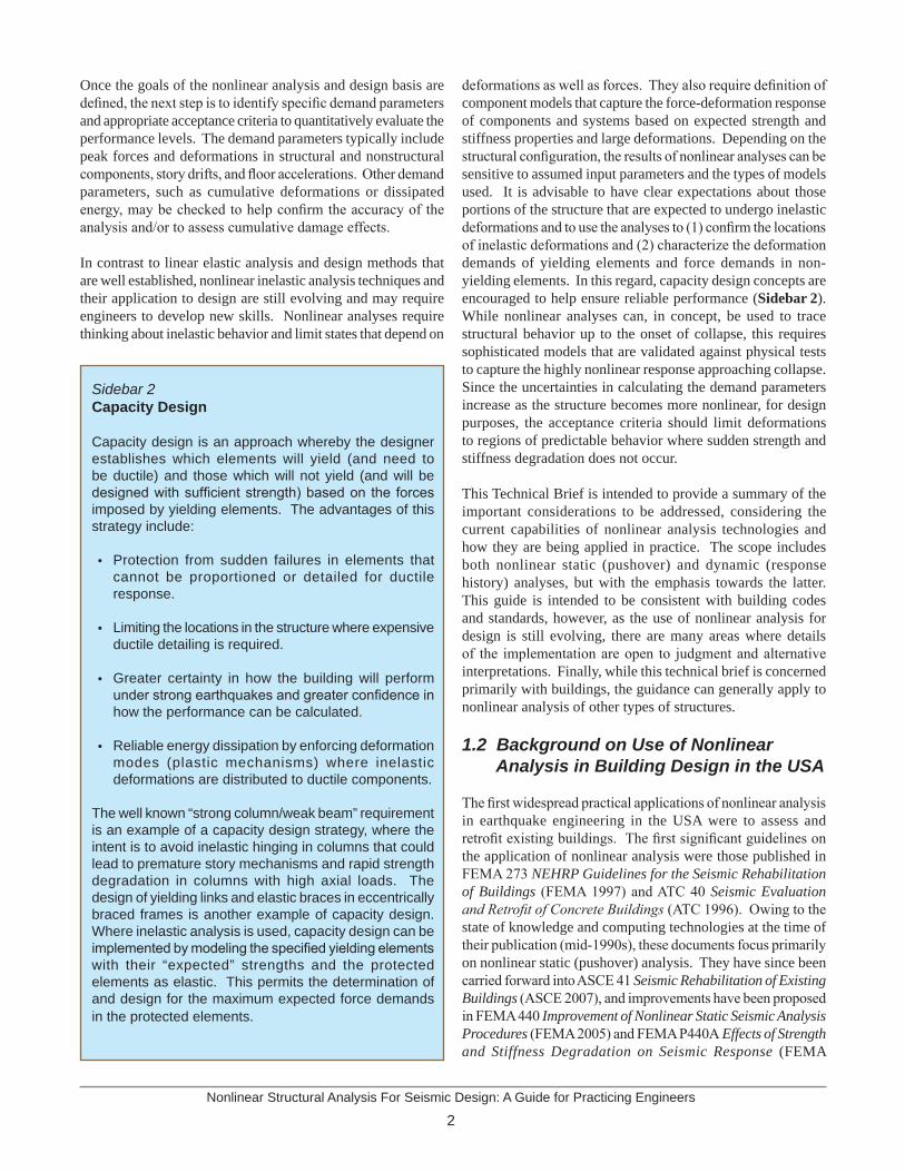
Disclaimers
The policy of the National Institute of Standards and Technology is to use the International System of Units (metric units) in all of its publications. However, in North America in the construction and building materials industry, certain non-SI units are so widely used instead of SI units that it is more practical and less confusing to include measurement values for customary units only in this publication.
This publication was produced as part of contract SB134107CQ0019, Task Order 69195 with the National Institute of Standards and Technology. The contents of this publication do not necessarily reflect the views or policies of the National Institute of Standards and Technology or the US Government.
This Technical Brief was produced under contract to NIST by the NEHRP Consultants Joint Venture, a joint venture of the Applied Technology Council (ATC) and the Consortium of Universities for Research in Earthquake Engineering (CUREE). While endeavoring to provide practical and accurate information in this publication, the NEHRP Consultants Joint Venture, the authors, and the reviewers do not assume liability for, nor make any expressed or implied warranty with regard to, the use of its information. Users of the information in this publication assume all liability arising from such use.
Cover photo – Nonlinear analysis model for a seismic retrofit study of an existing building with concrete shear walls.
How to Cite This PublicationDeierlein, Gregory G., Reinhorn, Andrei M., and Willford, Michael R. (2010). “Nonlinear structural analysis for seismic design,” NEHRP Seismic Design Technical Brief No. 4, produced by the NEHRP Consultants Joint Venture, a partnership of the Applied Technology Council and the Consortium of Universities for Research in Earthquake Engineering, for the National Institute of Standards and Technology, Gaithersburg, MD, NIST GCR 10-917-5.
Introduction..............................................................................................1Nonlinear Demand Parameters and Model Attributes.......................................4Modeling of Structural Components.............................................................12Foundations and Soil Structure Interaction...................................................19Requirements for Nonlinear Static Analysis..................................................21Requirements for Nonlinear Dynamic Analysis..............................................23References.............................................................................................27Notations and Abbreviations......................................................................30Credits....................................................................................................32
1. 2.3. 4. 5. 6. 7. 8. 9.
Contents
1Nonlinear Structural Analysis For Seismic Design: A Guide for Practicing Engineers
1.1 The Role and Use of Nonlinear Analysis in Seismic Design
While buildings are usually designed for seismic resistance using elastic analysis, most will experience significant inelastic deformations under large earthquakes. Modern performance-based design methods require ways to determine the realistic behavior of structures under such conditions. Enabled by advancements in computing technologies and available test data, nonlinear analyses provide the means for calculating structural response beyond the elastic range, including strength and stiffness deterioration associated with inelastic material behavior and large displacements. As such, nonlinear analysis can play an important role in the design of new and existing buildings.
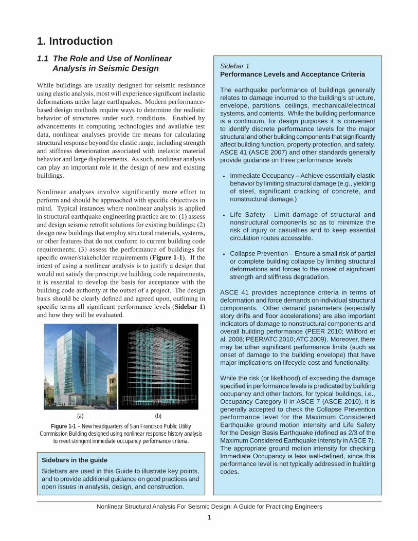
Nonlinear analyses involve significantly more effort to perform and should be approached with specific objectives in mind. Typical instances where nonlinear analysis is applied in structural earthquake engineering practice are to: (1) assess and design seismic retrofit solutions for existing buildings; (2) design new buildings that employ structural materials, systems, or other features that do not conform to current building code requirements; (3) assess the performance of buildings for specific owner/stakeholder requirements (Figure 1-1). If the intent of using a nonlinear analysis is to justify a design that would not satisfy the prescriptive building code requirements, it is essential to develop the basis for acceptance with the building code authority at the outset of a project. The design basis should be clearly defined and agreed upon, outlining in specific terms all significant performance levels (Sidebar 1) and how they will be evaluated.
1. Introduction
Sidebars in the guideSidebars are used in this Guide to illustrate key points, and to provide additional guidance on good practices and open issues in analysis, design, and construction.
Sidebar 1 Performance Levels and Acceptance Criteria
The earthquake performance of buildings generally relates to damage incurred to the building’s structure, envelope, partitions, ceilings, mechanical/electrical systems, and contents. While the building performance is a continuum, for design purposes it is convenient to identify discrete performance levels for the major structural and other building components that significantly affect building function, property protection, and safety. ASCE 41 (ASCE 2007) and other standards generally provide guidance on three performance levels:
Immediate Occupancy – Achieve essentially elastic behavior by limiting structural damage (e.g., yielding of steel, significant cracking of concrete, and nonstructural damage.)
Life Safety - Limit damage of structural and nonstructural components so as to minimize the risk of injury or casualties and to keep essential circulation routes accessible.
Collapse Prevention – Ensure a small risk of partial or complete building collapse by limiting structural deformations and forces to the onset of significant strength and stiffness degradation.
ASCE 41 provides acceptance criteria in terms of deformation and force demands on individual structural components. Other demand parameters (especially story drifts and floor accelerations) are also important indicators of damage to nonstructural components and overall building performance (PEER 2010; Willford et al. 2008; PEER/ATC 2010; ATC 2009). Moreover, there may be other significant performance limits (such as onset of damage to the building envelope) that have major implications on lifecycle cost and functionality.
While the risk (or likelihood) of exceeding the damage specified in performance levels is predicated by building occupancy and other factors, for typical buildings, i.e., Occupancy Category II in ASCE 7 (ASCE 2010), it is generally accepted to check the Collapse Prevention performance level for the Maximum Considered Earthquake ground motion intensity and Life Safety for the Design Basis Earthquake (defined as 2/3 of the Maximum Considered Earthquake intensity in ASCE 7). The appropriate ground motion intensity for checking Immediate Occupancy is less well-defined, since this performance level is not typically addressed in building codes.
•
•
•
Figure 1-1 – New headquarters of San Francisco Public Utility Commission Building designed using nonlinear response history analysis
to meet stringent immediate occupancy performance criteria.
(b)(a)
Nonlinear Structural Analysis For Seismic Design: A Guide for Practicing Engineers
2
Once the goals of the nonlinear analysis and design basis are defined, the next step is to identify specific demand parameters and appropriate acceptance criteria to quantitatively evaluate the performance levels. The demand parameters typically include peak forces and deformations in structural and nonstructural components, story drifts, and floor accelerations. Other demand parameters, such as cumulative deformations or dissipated energy, may be checked to help confirm the accuracy of the analysis and/or to assess cumulative damage effects.
In contrast to linear elastic analysis and design methods that are well established, nonlinear inelastic analysis techniques and their application to design are still evolving and may require engineers to develop new skills. Nonlinear analyses require thinking about inelastic behavior and limit states that depend on
Sidebar 2Capacity Design
Capacity design is an approach whereby the designer establishes which elements will yield (and need to be ductile) and those which will not yield (and will be designed with sufficient strength) based on the forces imposed by yielding elements. The advantages of this strategy include:
Protection from sudden failures in elements that cannot be proportioned or detailed for ductile response.
Limiting the locations in the structure where expensive ductile detailing is required.
Greater certainty in how the building will perform under strong earthquakes and greater confidence in how the performance can be calculated.
Reliable energy dissipation by enforcing deformation modes (plastic mechanisms) where inelastic deformations are distributed to ductile components.
The well known “strong column/weak beam” requirement is an example of a capacity design strategy, where the intent is to avoid inelastic hinging in columns that could lead to premature story mechanisms and rapid strength degradation in columns with high axial loads. The design of yielding links and elastic braces in eccentrically braced frames is another example of capacity design. Where inelastic analysis is used, capacity design can be implemented by modeling the specified yielding elements with their “expected” strengths and the protected elements as elastic. This permits the determination of and design for the maximum expected force demands in the protected elements.
deformations as well as forces. They also require definition of component models that capture the force-deformation response of components and systems based on expected strength and stiffness properties and large deformations. Depending on the structural configuration, the results of nonlinear analyses can be sensitive to assumed input parameters and the types of models used. It is advisable to have clear expectations about those portions of the structure that are expected to undergo inelastic deformations and to use the analyses to (1) confirm the locations of inelastic deformations and (2) characterize the deformation demands of yielding elements and force demands in non-yielding elements. In this regard, capacity design concepts are encouraged to help ensure reliable performance (Sidebar 2). While nonlinear analyses can, in concept, be used to trace structural behavior up to the onset of collapse, this requires sophisticated models that are validated against physical tests to capture the highly nonlinear response approaching collapse. Since the uncertainties in calculating the demand parameters increase as the structure becomes more nonlinear, for design purposes, the acceptance criteria should limit deformations to regions of predictable behavior where sudden strength and stiffness degradation does not occur.
This Technical Brief is intended to provide a summary of the important considerations to be addressed, considering the current capabilities of nonlinear analysis technologies and how they are being applied in practice. The scope includes both nonlinear static (pushover) and dynamic (response history) analyses, but with the emphasis towards the latter. This guide is intended to be consistent with building codes and standards, however, as the use of nonlinear analysis for design is still evolving, there are many areas where details of the implementation are open to judgment and alternative interpretations. Finally, while this technical brief is concerned primarily with buildings, the guidance can generally apply to nonlinear analysis of other types of structures.
1.2 Background on Use of Nonlinear Analysis in Building Design in the USA
The first widespread practical applications of nonlinear analysis in earthquake engineering in the USA were to assess and retrofit existing buildings. The first significant guidelines on the application of nonlinear analysis were those published in FEMA 273 NEHRP Guidelines for the Seismic Rehabilitation of Buildings (FEMA 1997) and ATC 40 Seismic Evaluation and Retrofit of Concrete Buildings (ATC 1996). Owing to the state of knowledge and computing technologies at the time of their publication (mid-1990s), these documents focus primarily on nonlinear static (pushover) analysis. They have since been carried forward into ASCE 41 Seismic Rehabilitation of Existing Buildings (ASCE 2007), and improvements have been proposed in FEMA 440 Improvement of Nonlinear Static Seismic Analysis Procedures (FEMA 2005) and FEMA P440A Effects of Strength and Stiffness Degradation on Seismic Response (FEMA
•
•
•
•
3Nonlinear Structural Analysis For Seismic Design: A Guide for Practicing Engineers
2009a). Note that while ASCE 41 and related documents have a primary focus on renovating existing buildings, the nonlinear analysis guidance and component modeling and acceptance criteria in these documents can be applied to new building design, provided that the chosen acceptance criteria provide performance levels expected for new building design in ASCE 7 (Sidebar 1).
About the same time that FEMA 273 and ATC 40 were under development, nonlinear analysis concepts were also being introduced into methods for seismic risk assessment, the most widely known being HAZUS (Kircher et al. 1997a; Kircher et al. 1997b; FEMA 2006). In particular, the building-specific loss assessment module of HAZUS employs nonlinear static analysis methods to develop earthquake damage fragility functions for buildings in the Earthquake Loss Estimation Methodology, HAZUS99-SR2, Advanced Engineering Building Module (FEMA 2002).
More recently, the role of nonlinear dynamic analysis for design is being expanded to quantify building performance more completely. The ATC 58 Guidelines for Seismic Performance Assessment of Buildings (ATC 2009) employ nonlinear dynamic analyses for seismic performance assessment of new and existing buildings, including fragility models that relate structural demand parameters to explicit damage and loss metrics. Nonlinear dynamic analyses are also being used to assess the performance of structural systems that do not conform to prescriptive seismic force-resisting system types in ASCE 7 Minimum Design Loads for Buildings and Other Structures (ASCE 2010). A significant impetus for this is in the design of tall buildings in high seismic regions, such as outlined in the following documents: Seismic Design Guidelines for Tall Buildings (PEER 2010), Recommendations for the Seismic Design of High-rise Buildings (Willford et al. 2008), and the PEER/ATC 72-1 Modeling and Acceptance Criteria for Seismic Design and Analysis of Tall Buildings (PEER/ATC 2010).
1.3 Definitions of Terms in this Guide While structural engineers familiar with the concept of nonlinear analysis for seismic design have been exposed to the following terms in a number of publications, the meanings of these terms have sometimes varied. The following definitions are used in this Guide.
Backbone Curve: Relationship between the generalized force and deformation (or generalized stress and strain) of a structural component or assembly that is used to characterize response in a nonlinear analysis model.
Cyclic Strength Degradation: Reduction in strength, measured at a given displacement loading cycles, due to reduction in yield strength and stiffness that occurs during the cyclic loading.
Cyclic Envelope: Curve of generalized force versus deformation that envelopes response data obtained from cyclic loading of a structural component or assembly.
In-Cycle Degradation: Reduction in strength that is associated with negative slop of load versus deflection plot within the same cycle in which yielding occurs.
Monotonic Curve: Curve of generalized force versus deformation data obtained from monotonic loading of a structural component or assembly.
Nonlinear Structural Analysis For Seismic Design: A Guide for Practicing Engineers
4
Figure 2-1 – Idealized models of beam-column elements.
2.1 Demand Parameters Modern performance-based seismic design entails setting performance levels and checking acceptance criteria for which a building is to be designed. Performance levels under defined intensities of ground shaking should be checked using appropriate demand parameters and acceptance criteria. The performance acceptance criteria may be specified for the overall systems, substructures, or components of a building.
For a given building and set of demand parameters, the structure must be modeled and analyzed so that the values of the demand parameters are calculated with sufficient accuracy for design purposes. The performance is checked by comparing the calculated values of demand parameters (in short the “demands”) to the acceptance criteria (“capacities”) for the desired performance level. The calculated demands and acceptance criteria are often compared through “demand-capacity” ratios. The acceptance criteria for seismic performance may vary depending on whether static or dynamic nonlinear analysis is used and how uncertainties associated with the demands and acceptance criteria are handled. For example, the component models, demand parameters, and acceptance criteria used in nonlinear static procedures need to implicitly account for cyclic degradation effects that are not modeled in the static analysis. On the other hand, some dynamic analysis models may directly incorporate degradation due to cyclic loading, in which case different models and acceptance criteria may be used.
Acceptance criteria for structural components generally distinguished between “deformation-controlled” (ductile components that can tolerate inelastic deformations) and “force-controlled” (non-ductile components whose capacities are governed by strength). In reality, most components exhibit some amount of inelastic deformation, and the distinction between force- and deformation-controlled components
2. Nonlinear Demand Parameters and Model Attributesis not absolute. Nevertheless, the distinction provides a practical approach to establish requirements for the analysis and design. Deformation-controlled components must be modeled as inelastic, whereas force-controlled components may be modeled as elastic, provided that the force demands do not imply significant yielding in the components. ASCE 41 defines deformation and strength acceptance criteria for Immediate Occupancy, Life Safety, and Collapse Prevention performance levels, and PEER/ATC 72-1 provides guidance on criteria for the onset of structural damage and significant strength/stiffness degradation.
Displacements, velocities, and accelerations are additional demand parameters that can provide insights into the overall building response and damage to nonstructural components and contents. Story racking deformations (which can often be approximated as story drift ratios) provide a good measure of overall structural response, including the vertical distribution of deformations and global torsion of the building, and demands in deformation-sensitive components, such as the building façade, interior partitions, or flexible piping systems. Peak floor accelerations and velocities are commonly used to design and assess performance of stiff acceleration-sensitive building components, such as rigidly anchored equipment, raised floor systems, braced ceiling systems, and rigid piping systems.
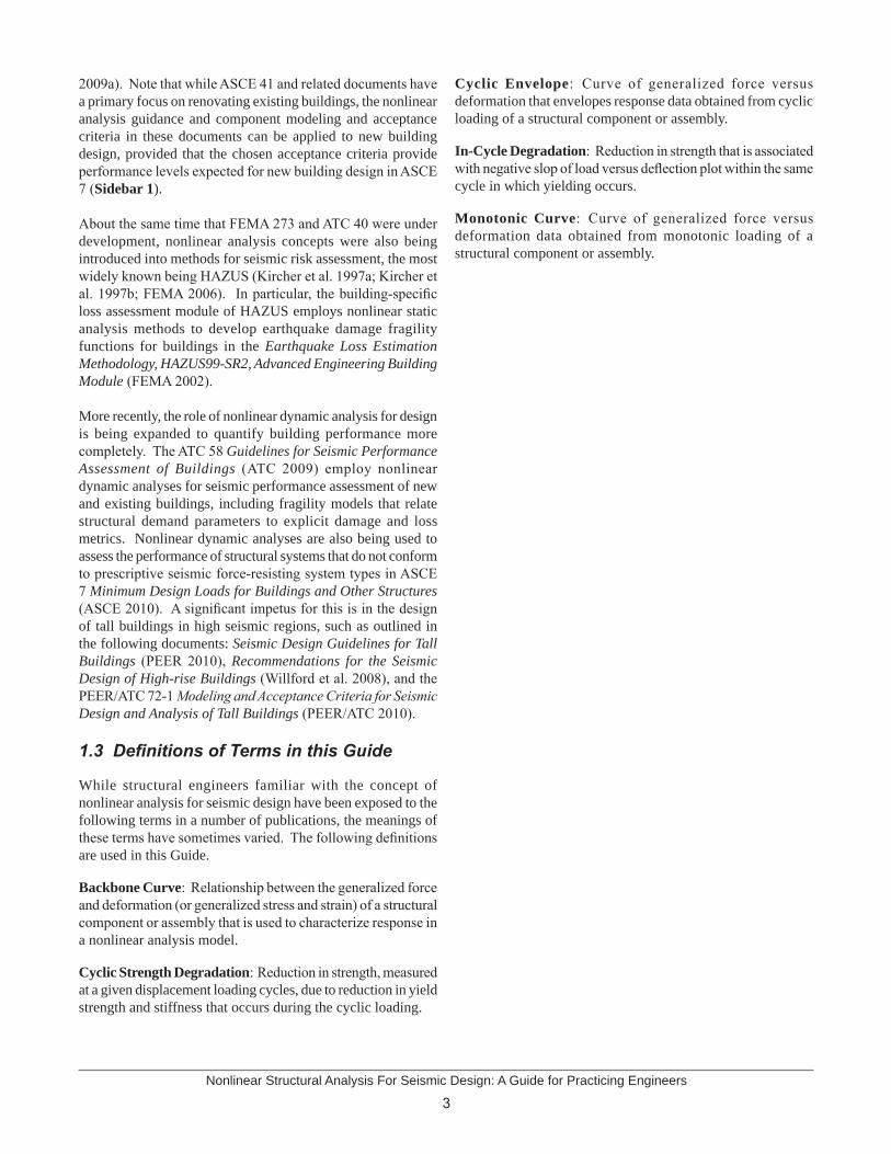
2.2 Structural Analysis Model Types Inelastic structural component models can be differentiated by the way that plasticity is distributed through the member cross sections and along its length. For example, shown in Figure 2-1 is a comparison of five idealized model types for simulating the inelastic response of beam-columns. Several types of structural members (e.g., beams, columns, braces, and some flexural walls) can be modeled using the concepts illustrated in Figure 2-1:
5Nonlinear Structural Analysis For Seismic Design: A Guide for Practicing Engineers
The simplest models concentrate the inelastic deformations at the end of the element, such as through a rigid-plastic hinge (Figure 2-1a) or an inelastic spring with hysteretic properties (Figure 2-1b). By concentrating the plasticity in zero-length hinges with moment-rotation model parameters, these elements have relatively condensed numerically efficient formulations.
The finite length hinge model (Figure 2-1c) is an efficient distributed plasticity formulation with designated hinge zones at the member ends. Cross sections in the inelastic hinge zones are characterized through either nonlinear moment-curvature relationships or explicit fiber-section integrations that enforce the assumption that plane sections remain plane. The inelastic hinge length may be fixed or variable, as determined from the moment-curvature characteristics of the section together with the concurrent moment gradient and axial force. Integration of deformations along the hinge length captures the spread of yielding more realistically than the concentrated hinges, while the finite hinge length facilitates calculation of hinge rotations.
The fiber formulation (Figure 2-1d) models distribute plasticity by numerical integrations through the member cross sections and along the member length. Uniaxial material models are defined to capture the nonlinear hysteretic axial stress-strain characteristics in the cross sections. The plane-sections-remain-plane assumption is enforced, where uniaxial material “fibers” are numerically integrated over the cross section to obtain stress resultants (axial force and moments) and incremental moment-curvature and axial force-strain relations. The cross section parameters are then integrated numerically at discrete sections along the member length, using displacement or force interpolation functions (Kunnath et al. 1990, Spacone et al. 1996). Distributed fiber formulations do not generally report plastic hinge rotations, but instead report strains in the steel and concrete cross section fibers. The calculated strain demands can be quite sensitive to the moment gradient, element length, integration method, and strain hardening parameters on the calculated strain demands. Therefore, the strain demands and acceptance criteria should be benchmarked against concentrated hinge models, for which rotation acceptance criteria are more widely reported.
The most complex models (Figure 2-1e) discretize the continuum along the member length and through the cross sections into small (micro) finite elements with nonlinear hysteretic constitutive properties that have numerous input parameters. This fundamental level of modeling offers the most versatility, but it also presents the most challenge in terms of model parameter calibration and computational resources. As with the fiber formulation, the strains calculated from the finite elements can be difficult to
Sidebar 3: Distributed Versus Concentrated Plasticity Elements
While distributed plasticity formulations (Figures 2-1c to 2-1e) model variations of the stress and strain through the section and along the member in more detail, important local behaviors, such as strength degradation due to local buckling of steel reinforcing bars or flanges, or the nonlinear interaction of flexural and shear, are difficult to capture without sophisticated and numerically intensive models. On the other hand, phenomenological concentrated hinge/spring models (Figure 2-1a and 2-1b), may be better suited to capturing the nonlinear degrading response of members through calibration using member test data on phenomenological moment-rotations and hysteresis curves. Thus, when selecting analysis model types, it is important to understand (1) the expected behavior, (2) the assumptions, and (3) the approximations inherent to the proposed model type. While more sophisticated formulations may seem to offer better capabilities for modeling certain aspects of behavior, simplified models may capture more effectively the relevant feature with the same or lower approximation. It is best to gain knowledge and confidence in specific models and software implementations by analyzing small test examples, where one can interrogate specific behavioral effects.
interpret relative to acceptance criteria that are typically reported in terms of hinge rotations and deformations.
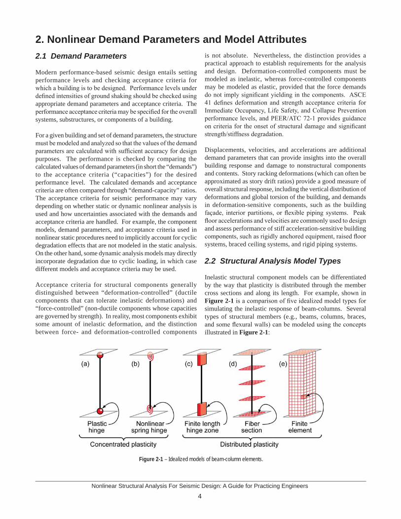
Concentrated and finite length hinge models (Figures 2-1a through Figure 2-1c) may consider the axial force-moment (P-M) interactions through yield surfaces (see Figure 2-2). On the other hand, fiber (Figure 2-1d) and finite element (Figure 2-1e) models capture the P-M response directly. Note that while the detailed fiber and finite element models can simulate certain behavior more fundamentally, they are not necessarily capable of modeling other effects, such as degradation due to reinforcing bar buckling and fracture that can be captured by simpler phenomenological models (Sidebar 3).
Some types of concentrated hinge models employ axial load-moment (P-M) yield surfaces. Whereas these models generally do a good job at tracking the initiation of yielding under axial load and bending, they may not capture accurately the post-yield and degrading response. On the other hand, some hinge elements with detailed moment-rotation hysteresis models (Figure 2-3) may not capture P-M interaction, except to the extent that the moment-rotation response is defined based on average values of axial load and shear that are assumed to be present in the hinge. A simple check on the model capabilities
•
•
•
•
Nonlinear Structural Analysis For Seismic Design: A Guide for Practicing Engineers
6
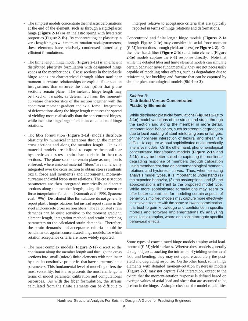
Figure 2-3 – Types of hysteretic modeling.
Figure 2-2 – Idealized axial-force-moment demands and strength interaction surfaces.
(a) Steel columns (b) Concrete walls and columns
(a) Hysteretic model without deterioration
(b) Model with stiffness degradation
(c) Model with cyclic strength degradation
(d) Model with fracture strength degradation
(e) Model with post-capping gradual strength deterioration
(f) Model with bond slip or crack closure (pinching)
7Nonlinear Structural Analysis For Seismic Design: A Guide for Practicing Engineers
is to analyze a concrete column under a low and high value of axial load (above and below the compression failure balance point) to examine whether the model tracks how the axial load affects the differences in rotation capacity and post-peak degradation. A further check would be to vary the axial loading during the analysis to see how well the effect of the changing axial load is captured.
Sidebar 4 Monotonic Versus Cyclic Envelope Curve
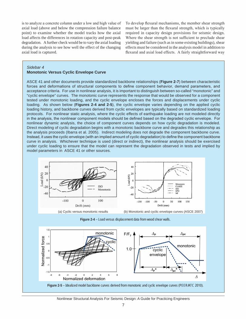
ASCE 41 and other documents provide standardized backbone relationships (Figure 2-7) between characteristic forces and deformations of structural components to define component behavior, demand parameters, and acceptance criteria. For use in nonlinear analysis, it is important to distinguish between so-called “monotonic” and “cyclic envelope” curves. The monotonic curve represents the response that would be observed for a component tested under monotonic loading, and the cyclic envelope encloses the forces and displacements under cyclic loading. As shown below (Figures 2-4 and 2-5), the cyclic envelope varies depending on the applied cyclic loading history, and backbone curves derived from cyclic envelopes are typically based on standardized loading protocols. For nonlinear static analysis, where the cyclic effects of earthquake loading are not modeled directly in the analysis, the nonlinear component models should be defined based on the degraded cyclic envelope. For nonlinear dynamic analysis, the choice of component curves depends on how cyclic degradation is modeled. Direct modeling of cyclic degradation begins with a monotonic backbone curve and degrades this relationship as the analysis proceeds (Ibarra et al. 2005). Indirect modeling does not degrade the component backbone curve. Instead, it uses the cyclic envelope (with an implied amount of cyclic degradation) to define the component backbone curve in analysis. Whichever technique is used (direct or indirect), the nonlinear analysis should be exercised under cyclic loading to ensure that the model can represent the degradation observed in tests and implied by model parameters in ASCE 41 or other sources.
To develop flexural mechanisms, the member shear strength must be larger than the flexural strength, which is typically required in capacity design provisions for seismic design. Where the shear strength is not sufficient to preclude shear yielding and failure (such as in some existing buildings), shear effects must be considered in the analysis model in addition to flexural and axial load effects. A fairly straightforward way
Figure 2-4 – Load versus displacement data from wood shear walls.
Figure 2-5 – Idealized model backbone curves derived from monotonic and cyclic envelope curves (PEER/ATC 2010).
(b) Monotonic and cyclic envelope curves (ASCE 2007)(a) Cyclic versus monotonic results
Nonlinear Structural Analysis For Seismic Design: A Guide for Practicing Engineers
8
Sidebar 5 Cyclic Versus In-cycle Degradation
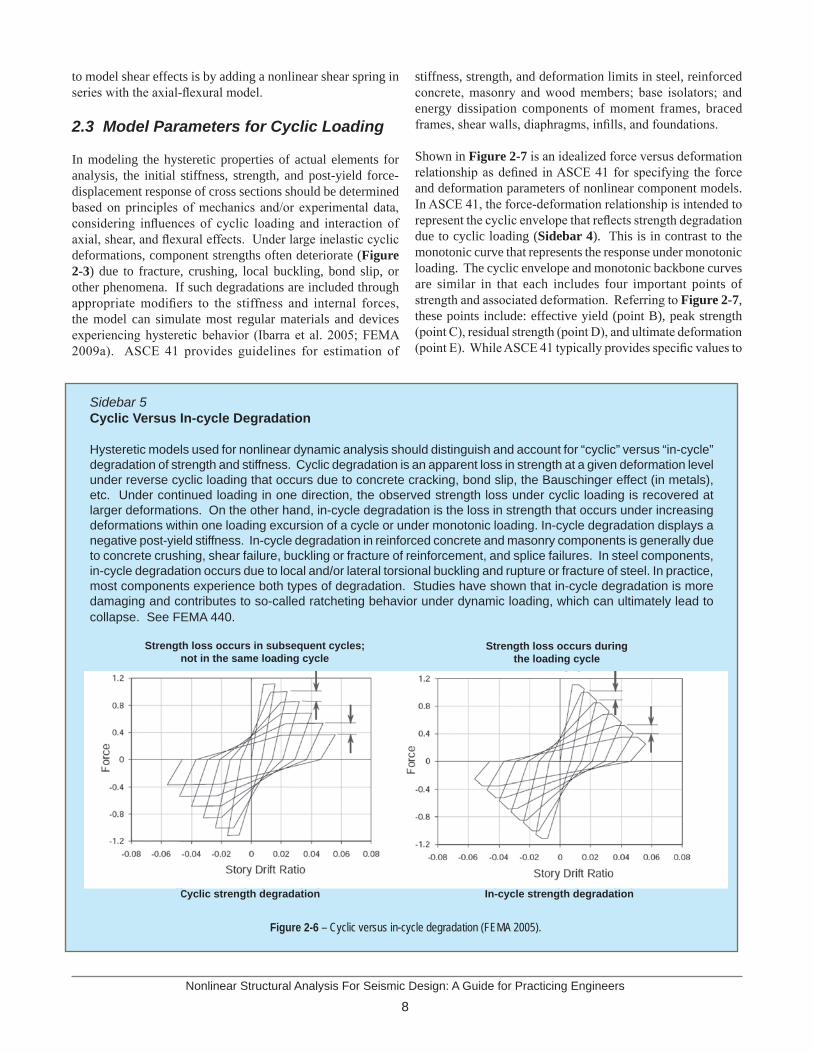
Hysteretic models used for nonlinear dynamic analysis should distinguish and account for “cyclic” versus “in-cycle” degradation of strength and stiffness. Cyclic degradation is an apparent loss in strength at a given deformation level under reverse cyclic loading that occurs due to concrete cracking, bond slip, the Bauschinger effect (in metals), etc. Under continued loading in one direction, the observed strength loss under cyclic loading is recovered at larger deformations. On the other hand, in-cycle degradation is the loss in strength that occurs under increasing deformations within one loading excursion of a cycle or under monotonic loading. In-cycle degradation displays a negative post-yield stiffness. In-cycle degradation in reinforced concrete and masonry components is generally due to concrete crushing, shear failure, buckling or fracture of reinforcement, and splice failures. In steel components, in-cycle degradation occurs due to local and/or lateral torsional buckling and rupture or fracture of steel. In practice, most components experience both types of degradation. Studies have shown that in-cycle degradation is more damaging and contributes to so-called ratcheting behavior under dynamic loading, which can ultimately lead to collapse. See FEMA 440.
to model shear effects is by adding a nonlinear shear spring in series with the axial-flexural model.
2.3 Model Parameters for Cyclic Loading
In modeling the hysteretic properties of actual elements for analysis, the initial stiffness, strength, and post-yield force-displacement response of cross sections should be determined based on principles of mechanics and/or experimental data, considering influences of cyclic loading and interaction of axial, shear, and flexural effects. Under large inelastic cyclic deformations, component strengths often deteriorate (Figure 2-3) due to fracture, crushing, local buckling, bond slip, or other phenomena. If such degradations are included through appropriate modifiers to the stiffness and internal forces, the model can simulate most regular materials and devices experiencing hysteretic behavior (Ibarra et al. 2005; FEMA 2009a). ASCE 41 provides guidelines for estimation of
stiffness, strength, and deformation limits in steel, reinforced concrete, masonry and wood members; base isolators; and energy dissipation components of moment frames, braced frames, shear walls, diaphragms, infills, and foundations.
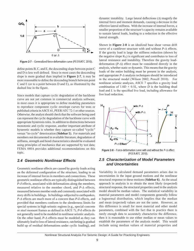
Shown in Figure 2-7 is an idealized force versus deformation relationship as defined in ASCE 41 for specifying the force and deformation parameters of nonlinear component models. In ASCE 41, the force-deformation relationship is intended to represent the cyclic envelope that reflects strength degradation due to cyclic loading (Sidebar 4). This is in contrast to the monotonic curve that represents the response under monotonic loading. The cyclic envelope and monotonic backbone curves are similar in that each includes four important points of strength and associated deformation. Referring to Figure 2-7, these points include: effective yield (point B), peak strength (point C), residual strength (point D), and ultimate deformation (point E). While ASCE 41 typically provides specific values to
Figure 2-6 – Cyclic versus in-cycle degradation (FEMA 2005).
Cyclic strength degradation In-cycle strength degradation
Strength loss occurs in subsequent cycles; not in the same loading cycle
Strength loss occurs duringthe loading cycle
9Nonlinear Structural Analysis For Seismic Design: A Guide for Practicing Engineers
define points B, C, and E, the descending slope between point C and D is less well defined. Since in most cases the descending slope is more gradual than implied in Figure 2-7, it may be more reasonable to define the descending branch between point C and E (or to a point between D and E), as illustrated by the dashed line in the figure.
Since models that capture cyclic degradation of the backbone curve are not yet common in commercial analysis software, in most cases it is appropriate to define modeling parameters to reproduce component cyclic envelope curves for tests or published criteria in ASCE 41, PEER/ATC 72-1 or other sources. Otherwise, the analyst should check that the software being used can represent the cyclic degradation of the backbone curve with appropriate hysteresis rules. In addition to distinctions between monotonic and cyclic response, another important attribute of hysteretic models is whether they capture so-called “cyclic” versus “in-cycle” deterioration (Sidebar 5). For materials and members not documented in available literature, degradation of stiffness, strength and bond characteristics should be evaluated using principles of mechanics that are supported by test data; FEMA 440A provides additional recommendations on this topic.
2.4 Geometric Nonlinear Effects
Geometric nonlinear effects are caused by gravity loads acting on the deformed configuration of the structure, leading to an increase of internal forces in members and connections. These geometric nonlinear effects are typically distinguished between P-d effects, associated with deformations along the members, measured relative to the member chord, and P-D effects, measured between member ends and commonly associated with story drifts in buildings. In buildings subjected to earthquakes, P-D effects are much more of a concern than P-d effects, and provided that members conform to the slenderness limits for special systems in high seismic regions (e.g., special concrete or steel moment frames as defined in ASCE 7), P-d effects do not generally need to be modeled in nonlinear seismic analysis. On the other hand, P-D effects must be modeled as they can ultimately lead to loss of lateral resistance, ratcheting (a gradual build up of residual deformations under cyclic loading), and
Figure 2-7 – Generalized force-deformation curve (PEER/ATC 2010).
dynamic instability. Large lateral deflections (D) magnify the internal force and moment demands, causing a decrease in the effective lateral stiffness. With the increase of internal forces, a smaller proportion of the structure’s capacity remains available to sustain lateral loads, leading to a reduction in the effective lateral strength.
Shown in Figure 2-8 is an idealized base shear versus drift curve of a cantilever structure with and without P-D effects. If the gravity load is large the stiffness reduction (shown by the negative slope KN) is significant and contributes to loss of lateral resistance and instability. Therefore the gravity load-deformation (P-D) effect must be considered directly in the analysis, whether static or dynamic. This means that the gravity loads of the entire building must be present in the analysis, and appropriate P-D analysis techniques should be introduced in the structural model (Wilson 2002; Powell 2010). For nonlinear seismic analyses, ASCE 7 specifies a gravity load combination of 1.0D + 0.5L, where D is the building dead load and L is the specified live load, including allowance for live load reduction.
Figure 2-8 – Force-deformation curve with and without the P-D effect (PEER/ATC 2010).
2.5 Characterization of Model Parameters and Uncertainties
Variability in calculated demand parameters arises due to uncertainties in the input ground motions and the nonlinear structural response to these motions (Sidebar 6). As the usual approach in analysis is to obtain the most likely (expected) structural response, the structural properties used in the analysis model should be median values. The statistical variability in material parameters and model components generally follow a lognormal distribution, which implies that the median and mean (expected) values are not the same. However, as this difference is small for most material and other model parameters, combined with the fact that in practice there is rarely enough data to accurately characterize the difference, then it is reasonable to use either median or mean values to establish the parameters of the analysis model. This would include using median values of material properties and
Nonlinear Structural Analysis For Seismic Design: A Guide for Practicing Engineers
10
component test data (such as the nonlinear hysteretic response data of a flexural hinge) to calibrate the analysis models. ASCE 41 and other standards provide guidance to relate minimum specified material properties to expected values, e.g., AISC 341 (AISC 2010) specifies Ry values to relate expected to minimum specified material strengths. By using median or mean values for a given earthquake intensity, the calculated values of demand parameters are median (50th percentile) estimates.
2.6 Quality Assurance
Nonlinear analysis software is highly sophisticated, requiring training and experience to obtain reliable results. While the analysis program’s technical users manual is usually the best resource on the features and use of any software, it may not provide a complete description of the outcome of various combinations of choices of input parameters, or the theoretical and practical limitations of different features. Therefore, analysts should build up experience of the software capabilities by performing analysis studies on problems of increasing scope and complexity, beginning with element tests of simple cantilever models and building up to models that encompass features relevant to the types of structures being analyzed. Basic checks should be made to confirm that the strength and stiffness of the model is correct under lateral load. Next, quasi-static cyclic tests should be run to confirm the nature of the hysteretic behavior, sensitivity tests with alternative input parameters, and evaluation of cyclic versus in-cycle degradation (Sidebar 5). Further validations using published experimental tests can help build understanding and confidence in the nonlinear analysis software and alternative modeling decisions (e.g., effects of element mesh refinement and section discretization).
Beyond having confidence in the software capabilities and the appropriate modeling techniques, it is essential to check the accuracy of models developed for a specific project. Checks begin with basic items necessary for any analysis. However, for nonlinear analyses additional checks are necessary to help ensure that the calculated responses are realistic. Sidebar 7 gives some suggestions in this regard.
Sidebar 6 Uncertainties in Seismic Assessment
The total variability in earthquake-induced demands is large and difficult to quantify. Considering all major sources of uncertainties, the coefficients of variation in demand parameters are on the order of 0.5 to 0.8 and generally increase with ground motion intensity. The variability is usually largest for structural deformations and accelerations and lower in force-controlled components of capacity-designed structures where the forces are limited by the strengths of yielding members. The variability is generally attributed to three main sources: (1) hazard uncertainty in the ground motion intensity, such as the spectral acceleration intensity calculated for a specified earthquake scenario or return period, (2) ground motion uncertainty arising from frequency content and duration of a ground motions with a given intensity, and (3) structural behavior and modeling uncertainties arising from the variability in (i) physical attributes of the structure such as material properties, geometry, structural details, etc., (ii) nonlinear behavior of the structural components and system, and (iii) mathematical model representation of the actual behavior. Through realistic modeling of the underlying mechanics, nonlinear dynamic analyses reduce uncertainty in demand predictions, as compared to nonlinear or linear static analyses where the underlying uncertainties are masked by simplified analysis assumptions. However, even with nonlinear dynamic analyses it is practically impossible to calculate accurately the variability in demand parameters. In concept it is possible to quantify the corresponding variability in the calculated demands using techniques such as Monte Carlo simulation. However, complete characterization of modeling uncertainty is a formidable problem for real building structures. Apart from the lack of necessary data to characterize fully the variability of the model parameters (standard deviations and correlations between multiple parameters), the number of analyses required to determine the resulting variability is prohibitive for practical assessment of real structures. Therefore, nonlinear analysis procedures are generally aimed at calculating the median (or mean) demands. Uncertainties in the evaluation are then accounted for (1) through the choice of the specified hazard level (return period) at which the analysis is run, and/or (2) the specified acceptance criteria to which the demands are compared. Separate factors or procedures are sometimes applied to check acceptance criteria for force-controlled or other capacity designed components.
11Nonlinear Structural Analysis For Seismic Design: A Guide for Practicing Engineers
Sidebar 7 Quality Assurance of Building Analysis Models Beyond familiarizing oneself with the capabilities of a specific software package, the following are suggested checks to help ensure the accuracy of nonlinear analysis models for calculating earthquake demand parameters:
Check the elastic modes of model. Ensure that the first mode periods for the translational axes and for rotation are consistent with expectation (e.g., hand calculation, preliminary structural models) and that the sequence of modes is logical. Check for spurious local modes that may be due to incorrect element properties, inadequate restraints, or incorrect mass definitions.
Check the total mass of the model and that the effective masses of the first few modes in each direction are realistic and account for most of the total mass.
Generate the elastic (displacement) response spectra of the input ground motion records. Check that they are consistent and note the variability between records. Determine the median spectrum of the records and the variability about the median.
Perform elastic response spectrum (using the median spectrum of the record set) and dynamic response history analyses of the model, and calculate the displacements at key positions and the elastic base shear and overturning moment. Compare the response spectrum results to the median of the dynamic analysis results.
Perform nonlinear static analyses to the target displacements for the median spectrum of the ground motion record set. Calculate the displacements at key positions and the base shear and overturning moment and compare to the elastic analysis results. Vary selected input or control parameters (e.g., with and without P-D, different loading patterns, variations in component strengths or deformation capacities) and confirm observed trends in the response.
Perform nonlinear dynamic analyses and calculate the median values of displacements, base shear, and overturning moment and compare to the results of elastic and nonlinear static analyses. Vary selected input or control parameters (similar to the variations applied in the static nonlinear analyses) and compare to each other and to the static pushover and elastic analyses. Plot hysteresis responses of selected components to confirm that they look realistic, and look for patterns in the demand parameters, including the distribution of deformations and spot checks of equilibrium.
•
•
•
•
•
•
Nonlinear Structural Analysis For Seismic Design: A Guide for Practicing Engineers
12
3. Modeling of Structural Components 3.1 Moment Frames (Flexural Beam-Columns)
Inelastic modeling of moment frame systems primarily involves component models for flexural members (beams and columns) and their connections. For systems that employ “special” moment frame capacity design principles, as defined in ASCE 7, the inelastic deformations should primarily occur in flexural hinges in the beams and the column bases. The NEHRP Seismic Design Technical Briefs by Moehle et al. (2008) and Hamburger et al. (2009) provide a summary of design concepts, criteria, and expected behavior for special concrete and steel moment frames. It is important to recognize, however, that the minimum design provisions of ASCE 7 and the underlying AISC 341 (2010) and ACI 318 (2008) standards for special moment frames do not always prevent hinging in the columns or inelastic panel zone deformations in beam-to-column joints. Therefore, the nonlinear model should include these effects, unless the actual demand-capacity ratios are small enough to prevent them. In frames that do not meet special moment frame requirements of ASCE 7, inelastic effects may occur in other locations, including member shear yielding, connection failure, and member instabilities due to local or lateral-torsional buckling.
Beam-columns are commonly modeled using either concentrated hinges or fiber-type elements. While the fiber elements generally enable more accurate modeling of the initiation of inelastic effects (steel yielding and concrete cracking) and spread of yielding, their ability may be limited to capture degradation associated with bond slip in concrete joints and local buckling and fracture of steel reinforcing bars and steel members. Concentrated hinge models, which can be calibrated to capture the overall force-deformation (or moment-rotation) response, including post-peak degradation, are often more
practical. Whatever the model type, the analysis should be capable of reproducing (under cyclic loading) the component cyclic envelope curves that are similar to those from tests or other published criteria, such as in ASCE 41 and PEER/ATC 72-1.
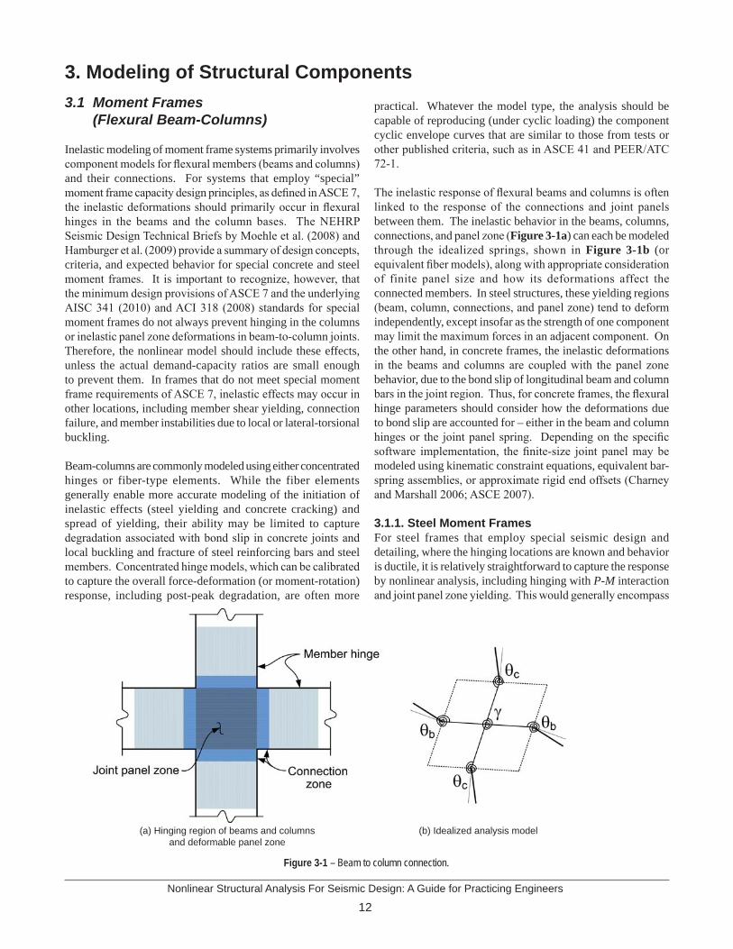
The inelastic response of flexural beams and columns is often linked to the response of the connections and joint panels between them. The inelastic behavior in the beams, columns, connections, and panel zone (Figure 3-1a) can each be modeled through the idealized springs, shown in Figure 3-1b (or equivalent fiber models), along with appropriate consideration of finite panel size and how its deformations affect the connected members. In steel structures, these yielding regions (beam, column, connections, and panel zone) tend to deform independently, except insofar as the strength of one component may limit the maximum forces in an adjacent component. On the other hand, in concrete frames, the inelastic deformations in the beams and columns are coupled with the panel zone behavior, due to the bond slip of longitudinal beam and column bars in the joint region. Thus, for concrete frames, the flexural hinge parameters should consider how the deformations due to bond slip are accounted for – either in the beam and column hinges or the joint panel spring. Depending on the specific software implementation, the finite-size joint panel may be modeled using kinematic constraint equations, equivalent bar-spring assemblies, or approximate rigid end offsets (Charney and Marshall 2006; ASCE 2007).
3.1.1. Steel Moment FramesFor steel frames that employ special seismic design and detailing, where the hinging locations are known and behavior is ductile, it is relatively straightforward to capture the response by nonlinear analysis, including hinging with P-M interaction and joint panel zone yielding. This would generally encompass
Figure 3-1 – Beam to column connection.
(b) Idealized analysis model(a) Hinging region of beams and columns and deformable panel zone
13Nonlinear Structural Analysis For Seismic Design: A Guide for Practicing Engineers
frames that conform to the special moment frame requirements of ASCE 7 and AISC 341 (Hamburger et al. 2009). Existing “pre-Northridge” moment frames, designed in high seismic regions of the Western U.S. according to older building code provisions, can be analyzed with similar models, provided that the beam/connection hinge ductility is reduced to account for potential fractures at the beam-to-column connection. Similarly, with appropriate adjustments to simulate the nonlinear moment-rotation behavior of connections, frames with partially restrained connections can be modeled. For steel frames composed of members with slender section properties and/or long unbraced lengths, nonlinear modeling is significantly more challenging due to the likelihood of local flange or web buckling and lateral-torsional buckling. This, combined with the fact that the inelastic rotation capacity of slender members is small, generally makes it less advantageous to use inelastic analysis for the design of steel frames with slender members. ASCE 41 provides some criteria for seismically non-conforming steel members, but as the cases covered are limited, one would need to look to other sources for data to establish models and criteria for frames with slender and otherwise non-conforming members.
3.1.2 Concrete Moment FramesConcrete frames that meet seismic design and detailing requirements and qualify as special moment frames are somewhat more difficult to model than steel frames. Stiffness of members is sensitive to concrete cracking, the joints are affected by concrete cracking and bond slip, and the post-yield response of columns and joint panels is sensitive to axial load. ASCE 41 (including supplement 1) and PEER/ATC 72-1 provide models and guidance for characterizing member stiffness, inelastic member hinge properties, and strategies for joint modeling. Lowes and Altoontash (2003) and Ghobarah and Biddah (1999) provide further details on modeling concrete beam-column joints. Frames that do not conform to the special seismic detailing but have behavior that is dominated by flexural
hinging can also be modeled, provided that the hinge properties and acceptance criteria are adjusted to account for their limited ductility. Frames with members that are susceptible to sudden shear failures or splice failures are more challenging to model. In such cases, nonlinear flexural models can be used to track response only up to the point where imposed shear force and/or splice force equals their respective strengths. Otherwise, to simulate further response, the analysis would need to capture the sudden degradation due to shear and splice failures.
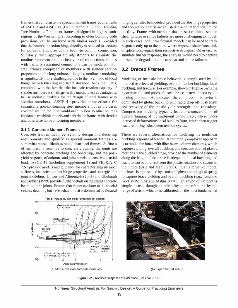
3.2 Braced Frames Modeling of inelastic brace behavior is complicated by the interactive effects of yielding, overall member buckling, local buckling, and fracture. For example, shown in Figure 3-2 is the hysteretic plot and photo of a steel brace, tested under a cyclic loading protocol. As indicated, the compression behavior is dominated by global buckling with rapid drop off in strength and recovery of the tensile yield strength upon reloading. Compression buckling typically leads to a concentration of flexural hinging at the mid-point of the brace, where under increased deformations local buckles form, which then trigger fracture during subsequent tension cycles.
There are several alternatives for modeling the nonlinear buckling response of braces. A commonly employed approach is to model the brace with fiber beam-column elements, which capture yielding, overall buckling, and concentration of plastic rotations in the buckled hinge, provided the number of elements along the length of the brace is adequate. Local buckling and fracture can be inferred from the plastic rotation and strains in the hinges (Uriz and Mahin 2008). In an alternative model, the brace is represented by a uniaxial phenomenological spring to capture brace yielding and overall buckling (e.g., Tang and Goel 1989; Uriz and Mahin 2008). This type of element is simple to use, though its reliability is more limited by the range of tests to which it is calibrated. In the most fundamental
Figure 3-2 – Nonlinear response of axial brace (Fell et al. 2010).
(b) Experimental set-up(a) Measured axial force-deformation
Nonlinear Structural Analysis For Seismic Design: A Guide for Practicing Engineers
14
analysis approach, the brace is modeled with continuum finite elements which can directly simulate yielding, overall buckling, and local buckling (Schachter and Reinhorn 2007). With appropriate material formulation, the finite element models can also simulate fracture initiation (Fell et al. 2010).
The axial-flexural fiber model, which provides a good compromise between modeling rigor and computational demands, requires calibration with test data to determine the appropriate number of elements, amplitude of initial out-of-straightness imperfections, and material hardening parameters. Uriz and Mahin (2008) found that the fiber approach gave reasonable results for the following model parameters: (1) brace subdivided into two or four elements, (2) initial geometric imperfection amplitude of 0.05 % to 0.1 % of the member length, and (3) ten to fifteen layers (fibers) through the cross section depth. For braces with compact sections as specified by AISC 341, local buckling is usually delayed enough to be insignificant until large deformations (story drifts on the order of 2 % to 4 %, depending on the brace compactness and slenderness). ASCE 41 provides acceptance criteria, described as a function of axial brace displacements, which can be obtained from the fiber-type beam-column models, phenomenological axial spring models, or finite element models.
3.2.1 Buckling-Restrained BracesIn contrast to conventional braces, buckling-restrained braces are straightforward to model with uniaxial nonlinear springs. Yield strength, cyclic strain hardening, and low-cycle fatigue endurance data are generally available from the brace manufacturers. Bi-linear force-deformation models are sufficiently accurate to capture the behavior. Acceptance criteria for the brace elements, based on peak deformations and cumulative deformations, can be inferred from the AISC 341 qualification testing requirements for buckling restrained braces.
3.3 Infill Walls and Panels
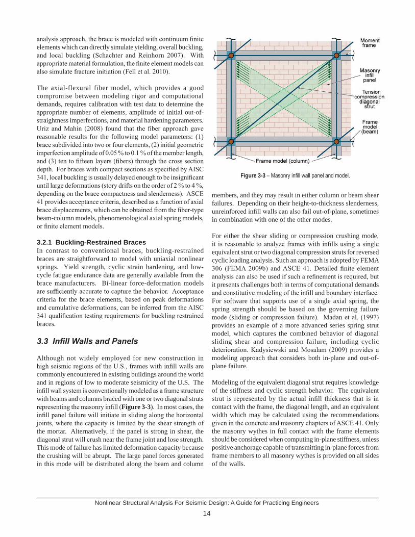
Although not widely employed for new construction in high seismic regions of the U.S., frames with infill walls are commonly encountered in existing buildings around the world and in regions of low to moderate seismicity of the U.S. The infill wall system is conventionally modeled as a frame structure with beams and columns braced with one or two diagonal struts representing the masonry infill (Figure 3-3). In most cases, the infill panel failure will initiate in sliding along the horizontal joints, where the capacity is limited by the shear strength of the mortar. Alternatively, if the panel is strong in shear, the diagonal strut will crush near the frame joint and lose strength. This mode of failure has limited deformation capacity because the crushing will be abrupt. The large panel forces generated in this mode will be distributed along the beam and column
members, and they may result in either column or beam shear failures. Depending on their height-to-thickness slenderness, unreinforced infill walls can also fail out-of-plane, sometimes in combination with one of the other modes.
For either the shear sliding or compression crushing mode, it is reasonable to analyze frames with infills using a single equivalent strut or two diagonal compression struts for reversed cyclic loading analysis. Such an approach is adopted by FEMA 306 (FEMA 2009b) and ASCE 41. Detailed finite element analysis can also be used if such a refinement is required, but it presents challenges both in terms of computational demands and constitutive modeling of the infill and boundary interface. For software that supports use of a single axial spring, the spring strength should be based on the governing failure mode (sliding or compression failure). Madan et al. (1997) provides an example of a more advanced series spring strut model, which captures the combined behavior of diagonal sliding shear and compression failure, including cyclic deterioration. Kadysiewski and Mosalam (2009) provides a modeling approach that considers both in-plane and out-of-plane failure.
Modeling of the equivalent diagonal strut requires knowledge of the stiffness and cyclic strength behavior. The equivalent strut is represented by the actual infill thickness that is in contact with the frame, the diagonal length, and an equivalent width which may be calculated using the recommendations given in the concrete and masonry chapters of ASCE 41. Only the masonry wythes in full contact with the frame elements should be considered when computing in-plane stiffness, unless positive anchorage capable of transmitting in-plane forces from frame members to all masonry wythes is provided on all sides of the walls.
Figure 3-3 – Masonry infill wall panel and model.
15Nonlinear Structural Analysis For Seismic Design: A Guide for Practicing Engineers
3.4 Shear Walls Reinforced concrete shear walls are commonly employed in seismic lateral-force-resisting systems for buildings. They may take the form of isolated planar walls, flanged walls (often C-, I- or T-shaped in plan) and larger three dimensional assemblies such as building cores. Nearby walls are often connected by coupling beams for greater structural efficiency where large openings for doorways are required. The seismic behavior of shear walls is often distinguished between slender (ductile flexure governed) or squat (shear governed) according to the governing mode of yielding and failure. In general, it is desirable to achieve ductile flexural behavior, but this is not possible in circumstances such as (1) short walls with high shear-to-flexure ratios that are susceptible to shear failures, (2) bearing walls with high axial stress and/or inadequate confinement that are susceptible to compression failures, and (3) in existing buildings without seismic design and detailing qualifying the wall system as special as defined in ASCE 7.
Cyclic and shake table tests on reinforced concrete shear walls reveal a number of potential failure modes that simple models cannot represent explicitly, however these failure modes are generally reflected in the backbone curves, hysteresis rules, and performance criteria adopted in lumped plasticity models. These failure modes include (1) rebar bond failure and lap splice slip, (2) concrete spalling, rebar buckling, and loss of confinement, (3) rebar fracture on straightening of buckle, and (4) combined shear and compression failure at wall toe. Some of these failure modes can be captured, either explicitly or implicitly, in fiber and finite element type modeling approaches.
3.4.1 Modeling of Slender WallsSlender concrete shear walls detailed to current seismic design requirements, having low axial stress, and designed with sufficient shear strength to avoid shear failures, perform in a similar manner to reinforced concrete beam-columns. Ductile flexural behavior with stable hysteresis can develop up to hinge rotation limits that are a function of axial load and shear in the hinge region.
Subject to the cautions noted below, simple slender walls (including coupled walls) can be modeled as vertical beam-column elements with lumped flexural plastic hinges at the ends with reasonable accuracy and computational efficiency. The modeling parameters and plastic rotation limits of ASCE 41 may be used for guidance. The following points should be noted:
The lumped hinge models are only suitable for assessing performance within such allowable plastic hinge rotation limits as stable hysteresis occurs, considering axial and shear forces in the hinge.
Nonlinearity only arises at the designated hinge(s), and equivalent flexural and shear stiffness must be specified for elastic elements outside of the hinge. ASCE 41 and PEER/ATC 72-1 provide guidance on effective stiffness parameters that account for flexural and shear cracking to handle typical cases (i.e., planar walls with typical reinforcement, wall proportions, and gravity stresses).
The flexural strength may be estimated by the nominal strength provisions of ACI 318 using expected material properties and taking account of the axial load. Where the axial load varies significantly during loading (e.g., coupled shear walls) a P-M interaction surface (Figure 2-2) should be used rather than a constant flexural strength. Shear failure should be prevented in slender shear walls, and studies have shown (PEER/ATC 72-1) that standard seismic design criteria may underestimate the actual shear force demands. Therefore, it is best to perform the analysis to determine the shear force demands and then to design the wall to resist these demands, considering variability in the shear demands and capacities. Since shear strength varies with applied axial stress (which varies during an earthquake in coupled shear walls) it may be necessary to check the design at multiple time steps during nonlinear dynamic analyses.
Beam-column elements are more problematic to use in three-dimensional wall configurations with significant bi-directional interaction, particularly if the wall system is subjected to torsion.
Fiber-type models are commonly employed to model slender walls, where the wall cross section is discretized into a number of concrete and steel fibers. With appropriate material nonlinear axial stress-strain characteristics, the fiber wall models can capture with reasonable accuracy the variation of axial and flexural stiffness due to concrete cracking and steel yielding under varying axial and bending loads. A principal limitation of conventional beam-column element fiber formulations is the assumption that plane sections remain plane, such that shear lag effects associated with flexure and warping torsion are not captured. These effects may be significant in non-planar core wall configurations. This limitation may be alleviated through formulations that model the wall with two-dimensional shell-type finite elements. The fiber idealization can be implemented in the shell elements to integrate through the cross section for axial/flexural effects, but in-plane shear is uncoupled and remains elastic. The number of elements required across a wall segment width and over the wall height depends on the available element types, the wall proportions, and the bending moment gradient. In particular, the number of elements over the hinge length will impact the effective gage length of the calculated strains.
•
•
•
•
•
Nonlinear Structural Analysis For Seismic Design: A Guide for Practicing Engineers
16
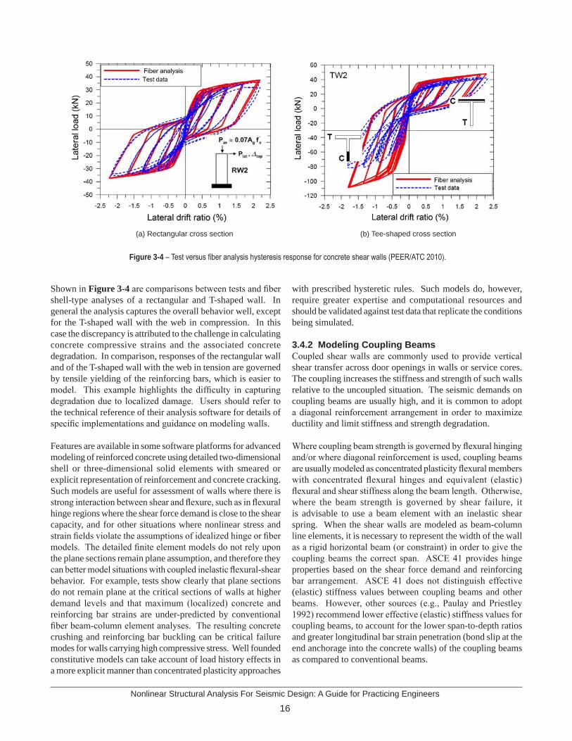
Shown in Figure 3-4 are comparisons between tests and fiber shell-type analyses of a rectangular and T-shaped wall. In general the analysis captures the overall behavior well, except for the T-shaped wall with the web in compression. In this case the discrepancy is attributed to the challenge in calculating concrete compressive strains and the associated concrete degradation. In comparison, responses of the rectangular wall and of the T-shaped wall with the web in tension are governed by tensile yielding of the reinforcing bars, which is easier to model. This example highlights the difficulty in capturing degradation due to localized damage. Users should refer to the technical reference of their analysis software for details of specific implementations and guidance on modeling walls.
Features are available in some software platforms for advanced modeling of reinforced concrete using detailed two-dimensional shell or three-dimensional solid elements with smeared or explicit representation of reinforcement and concrete cracking. Such models are useful for assessment of walls where there is strong interaction between shear and flexure, such as in flexural hinge regions where the shear force demand is close to the shear capacity, and for other situations where nonlinear stress and strain fields violate the assumptions of idealized hinge or fiber models. The detailed finite element models do not rely upon the plane sections remain plane assumption, and therefore they can better model situations with coupled inelastic flexural-shear behavior. For example, tests show clearly that plane sections do not remain plane at the critical sections of walls at higher demand levels and that maximum (localized) concrete and reinforcing bar strains are under-predicted by conventional fiber beam-column element analyses. The resulting concrete crushing and reinforcing bar buckling can be critical failure modes for walls carrying high compressive stress. Well founded constitutive models can take account of load history effects in a more explicit manner than concentrated plasticity approaches
with prescribed hysteretic rules. Such models do, however, require greater expertise and computational resources and should be validated against test data that replicate the conditions being simulated.
3.4.2 Modeling Coupling BeamsCoupled shear walls are commonly used to provide vertical shear transfer across door openings in walls or service cores. The coupling increases the stiffness and strength of such walls relative to the uncoupled situation. The seismic demands on coupling beams are usually high, and it is common to adopt a diagonal reinforcement arrangement in order to maximize ductility and limit stiffness and strength degradation.
Where coupling beam strength is governed by flexural hinging and/or where diagonal reinforcement is used, coupling beams are usually modeled as concentrated plasticity flexural members with concentrated flexural hinges and equivalent (elastic) flexural and shear stiffness along the beam length. Otherwise, where the beam strength is governed by shear failure, it is advisable to use a beam element with an inelastic shear spring. When the shear walls are modeled as beam-column line elements, it is necessary to represent the width of the wall as a rigid horizontal beam (or constraint) in order to give the coupling beams the correct span. ASCE 41 provides hinge properties based on the shear force demand and reinforcing bar arrangement. ASCE 41 does not distinguish effective (elastic) stiffness values between coupling beams and other beams. However, other sources (e.g., Paulay and Priestley 1992) recommend lower effective (elastic) stiffness values for coupling beams, to account for the lower span-to-depth ratios and greater longitudinal bar strain penetration (bond slip at the end anchorage into the concrete walls) of the coupling beams as compared to conventional beams.
Figure 3-4 – Test versus fiber analysis hysteresis response for concrete shear walls (PEER/ATC 2010).
(b) Tee-shaped cross section(a) Rectangular cross section
17Nonlinear Structural Analysis For Seismic Design: A Guide for Practicing Engineers
As with other cases where the model parameters are uncertain, it is recommended to investigate the sensitivity of the calculated demand parameters by conducting analyses for the expected range of coupling beam and wall model parameters.
3.4.3 Modeling Squat Shear WallsSquat shear walls fail in shear rather than flexure, and present significant modeling challenges. Monotonic tests show greater displacement ductility than can be relied upon in cyclic loading, where degradation of stiffness and strength (with highly pinched hysteresis loops) is observed. These behaviors are not easily captured using beam-column or fiber-type elements. Some analysis platforms contain suitable formulations comprising in-series nonlinear shear and flexure springs. In addition, detailed nonlinear reinforced concrete shell finite element formulations are available in some platforms, which can reproduce most observed features of behavior, though require careful calibration against test results.
3.5 Floors, Diaphragms, and Collectors
Floor diaphragms and collectors should be modeled to realistically represent the distribution of inertia loads from floors to the other elements of the lateral system and the redistribution of lateral forces among different parts of lateral system due to changes in configuration, relative stiffness, and/or relative strength. Floor diaphragms are often modeled as rigid, as this reduces the modeling and computational effort. This assumption is acceptable in many cases when the stresses and force transfers in the diaphragms are low relative to the diaphragm strength. However, the rigid modeling assumption is not always appropriate or the most convenient for design. The following questions should be considered:
How does the stiffness of the diaphragm compare with that of the vertically oriented components, including consideration of slab cracking where diaphragm stresses are high?
Would explicit modeling of diaphragms and collectors as flexible, using finite elements, facilitate the calculation of their design forces?
Will the rigid diaphragm constraint that suppresses axial deformations in framing members in the plane of the diaphragm distort the structural behavior, such as by eliminating the axial deformations of horizontal chords of braced lateral systems?
The adopted modeling approach should make a realistic representation of the stiffness of the diaphragm and collectors and enable the force demands to be extracted for design. Since concrete floor slabs may crack, it is difficult to make exact predictions of stiffness, particularly when (1) the reinforcement ratios are low, (2) the demands induce significant cracking, and/or (3) the slab is formed on profiled metal decking. If equivalent
•
•
•
linear stiffness parameters are used, the assumed stiffnesses should be reviewed in the light of the induced stresses and updated as necessary. Alternatively, where inelastic diaphragm effects are a major factor to the system behavior, nonlinear finite element formulations (membrane or shell) may be used. Analysis with upper and lower bound stiffness can also be useful to determine the sensitivity of the calculated behavior to variability in diaphragm stiffness.
The stiffness of floor beams (with slabs acting as “flanges”) framing with gravity columns can sometimes significantly increase the lateral stiffness of a structure even if the beams are designed as gravity framing only, and including them in the analysis can benefit the performance assessment of a design. A possible modeling technique is to include the grillage of primary floor beams and girders in the model as beam elements with two-dimensional shell or membrane elements to represent the in-plane stiffness of the diaphragm. In this case the slab may be modeled with a coarse mesh, and the stiffness and strength formulation of the beams in bending should include any desired interaction with the slab.
In accordance with ASCE 7, the collectors should be designed with sufficient strength to remain essentially elastic under the forces induced from earthquakes, and there is an argument (PEER/ATC 72-1) to design certain key diaphragms to remain essentially elastic as well. The calculated forces and stresses of seismic collectors should be interpreted with care. Membrane or shell finite elements in parallel with beams may take some of the “collector” force that a hand calculation would assign to the collector beam. Alternatively, where collectors are modeled as rigid (or very stiff elastic elements), the collector forces from dynamic analyses may be excessively large due to transient peaks, which would be damped out by minor yielding of the collector elements or their connections.
For further guidance on the analysis and design of reinforced concrete diaphragms refer to NEHRP Seismic Design Technical Brief No. 3 Seismic Design of Cast-in-Place Concrete Diaphragms, Chords, and Collectors (Moehle et al. 2010) and PEER/ATC 72-1. 3.6 Energy Dissipating Devices
Use of passive energy dissipation is an emerging technology that enhances building performance by reducing the demands through addition of damping devices and stiffening elements. In determining the seismic demand parameters, a nonlinear analysis model is required that can capture the forces, deformations, or other demand parameters for the devices. The analysis model of the device should account for its dependence on loading rates, temperature, sustained (gravity and other) loads, and other interactions. Multiple analyses may be necessary to capture and bound the effects of varying mechanical characteristics of the devices.
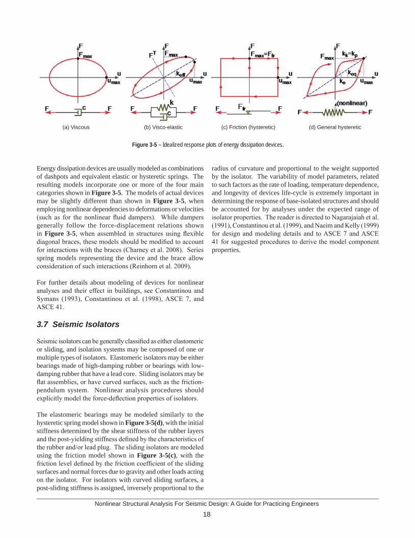
Nonlinear Structural Analysis For Seismic Design: A Guide for Practicing Engineers
18
Energy dissipation devices are usually modeled as combinations of dashpots and equivalent elastic or hysteretic springs. The resulting models incorporate one or more of the four main categories shown in Figure 3-5. The models of actual devices may be slightly different than shown in Figure 3-5, when employing nonlinear dependencies to deformations or velocities (such as for the nonlinear fluid dampers). While dampers generally follow the force-displacement relations shown in Figure 3-5, when assembled in structures using flexible diagonal braces, these models should be modified to account for interactions with the braces (Charney et al. 2008). Series spring models representing the device and the brace allow consideration of such interactions (Reinhorn et al. 2009).
For further details about modeling of devices for nonlinear analyses and their effect in buildings, see Constantinou and Symans (1993), Constantinou et al. (1998), ASCE 7, and ASCE 41.
3.7 Seismic Isolators
Seismic isolators can be generally classified as either elastomeric or sliding, and isolation systems may be composed of one or multiple types of isolators. Elastomeric isolators may be either bearings made of high-damping rubber or bearings with low-damping rubber that have a lead core. Sliding isolators may be flat assemblies, or have curved surfaces, such as the friction-pendulum system. Nonlinear analysis procedures should explicitly model the force-deflection properties of isolators.
The elastomeric bearings may be modeled similarly to the hysteretic spring model shown in Figure 3-5(d), with the initial stiffness determined by the shear stiffness of the rubber layers and the post-yielding stiffness defined by the characteristics of the rubber and/or lead plug. The sliding isolators are modeled using the friction model shown in Figure 3-5(c), with the friction level defined by the friction coefficient of the sliding surfaces and normal forces due to gravity and other loads acting on the isolator. For isolators with curved sliding surfaces, a post-sliding stiffness is assigned, inversely proportional to the
radius of curvature and proportional to the weight supported by the isolator. The variability of model parameters, related to such factors as the rate of loading, temperature dependence, and longevity of devices life-cycle is extremely important in determining the response of base-isolated structures and should be accounted for by analyses under the expected range of isolator properties. The reader is directed to Nagarajaiah et al. (1991), Constantinou et al. (1999), and Naeim and Kelly (1999) for design and modeling details and to ASCE 7 and ASCE 41 for suggested procedures to derive the model component properties.
Figure 3-5 – Idealized response plots of energy dissipation devices.
(a) Viscous (b) Visco-elastic (c) Friction (hysteretic) (d) General hysteretic
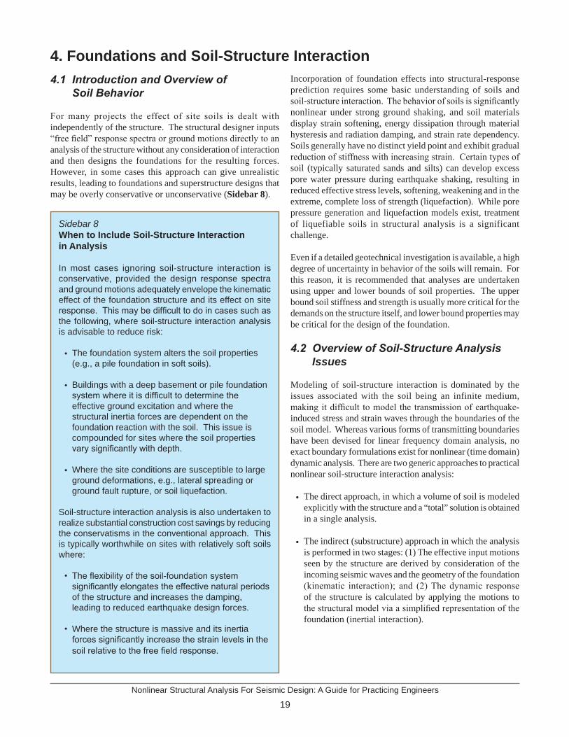
19Nonlinear Structural Analysis For Seismic Design: A Guide for Practicing Engineers
4. Foundations and Soil-Structure Interaction 4.1 Introduction and Overview of Soil Behavior
For many projects the effect of site soils is dealt with independently of the structure. The structural designer inputs “free field” response spectra or ground motions directly to an analysis of the structure without any consideration of interaction and then designs the foundations for the resulting forces. However, in some cases this approach can give unrealistic results, leading to foundations and superstructure designs that may be overly conservative or unconservative (Sidebar 8).
Incorporation of foundation effects into structural-response prediction requires some basic understanding of soils and soil-structure interaction. The behavior of soils is significantly nonlinear under strong ground shaking, and soil materials display strain softening, energy dissipation through material hysteresis and radiation damping, and strain rate dependency. Soils generally have no distinct yield point and exhibit gradual reduction of stiffness with increasing strain. Certain types of soil (typically saturated sands and silts) can develop excess pore water pressure during earthquake shaking, resulting in reduced effective stress levels, softening, weakening and in the extreme, complete loss of strength (liquefaction). While pore pressure generation and liquefaction models exist, treatment of liquefiable soils in structural analysis is a significant challenge.
Even if a detailed geotechnical investigation is available, a high degree of uncertainty in behavior of the soils will remain. For this reason, it is recommended that analyses are undertaken using upper and lower bounds of soil properties. The upper bound soil stiffness and strength is usually more critical for the demands on the structure itself, and lower bound properties may be critical for the design of the foundation.
4.2 Overview of Soil-Structure Analysis Issues
Modeling of soil-structure interaction is dominated by the issues associated with the soil being an infinite medium, making it difficult to model the transmission of earthquake-induced stress and strain waves through the boundaries of the soil model. Whereas various forms of transmitting boundaries have been devised for linear frequency domain analysis, no exact boundary formulations exist for nonlinear (time domain) dynamic analysis. There are two generic approaches to practical nonlinear soil-structure interaction analysis:
The direct approach, in which a volume of soil is modeled explicitly with the structure and a “total” solution is obtained in a single analysis.
The indirect (substructure) approach in which the analysis is performed in two stages: (1) The effective input motions seen by the structure are derived by consideration of the incoming seismic waves and the geometry of the foundation (kinematic interaction); and (2) The dynamic response of the structure is calculated by applying the motions to the structural model via a simplified representation of the foundation (inertial interaction).
Sidebar 8When to Include Soil-Structure Interaction in Analysis
In most cases ignoring soil-structure interaction is conservative, provided the design response spectra and ground motions adequately envelope the kinematic effect of the foundation structure and its effect on site response. This may be difficult to do in cases such as the following, where soil-structure interaction analysis is advisable to reduce risk:
The foundation system alters the soil properties (e.g., a pile foundation in soft soils).
Buildings with a deep basement or pile foundation system where it is difficult to determine the effective ground excitation and where the structural inertia forces are dependent on the foundation reaction with the soil. This issue is compounded for sites where the soil properties vary significantly with depth.
Where the site conditions are susceptible to large ground deformations, e.g., lateral spreading or ground fault rupture, or soil liquefaction.
Soil-structure interaction analysis is also undertaken to realize substantial construction cost savings by reducing the conservatisms in the conventional approach. This is typically worthwhile on sites with relatively soft soils where:
The flexibility of the soil-foundation system significantly elongates the effective natural periods of the structure and increases the damping, leading to reduced earthquake design forces.
Where the structure is massive and its inertia forces significantly increase the strain levels in the soil relative to the free field response.
•
•
•
•
•
•
•
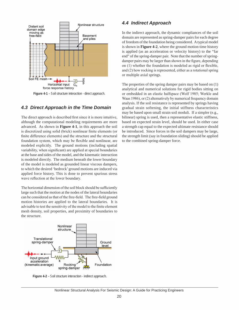
Nonlinear Structural Analysis For Seismic Design: A Guide for Practicing Engineers
20
4.3 Direct Approach in the Time Domain The direct approach is described first since it is more intuitive, although the computational modeling requirements are more advanced. As shown in Figure 4-1, in this approach the soil is discretized using solid (brick) nonlinear finite elements (or finite difference elements) and the structure and the structural foundation system, which may be flexible and nonlinear, are modeled explicitly. The ground motions (including spatial variability, when significant) are applied at special boundaries at the base and sides of the model, and the kinematic interaction is modeled directly. The medium beneath the lower boundary of the model is modeled as grounded linear viscous dampers, to which the desired ‘bedrock’ ground motions are induced via applied force history. This is done to prevent spurious stress wave reflection at the lower boundary.
The horizontal dimension of the soil block should be sufficiently large such that the motion at the nodes of the lateral boundaries can be considered as that of the free-field. The free-field ground motion histories are applied to the lateral boundaries. It is advisable to test the sensitivity of the model to the finite element mesh density, soil properties, and proximity of boundaries to the structure.
4.4 Indirect Approach
In the indirect approach, the dynamic compliances of the soil domain are represented as spring-damper pairs for each degree of freedom of the foundation being considered. A typical model is shown in Figure 4-2, where the ground motion time history is applied (as an acceleration or velocity history) to the “far end” of the spring-damper pair. Note that the number of spring-damper pairs may be larger than shown in the figure, depending on (1) whether the foundation is modeled as rigid or flexible, and (2) how rocking is represented, either as a rotational spring or multiple axial springs.
The properties of the spring damper pairs may be based on (1) analytical and numerical solutions for rigid bodies sitting on or embedded in an elastic halfspace (Wolf 1985; Werkle and Waas 1986), or (2) alternatively by numerical frequency domain analysis. If the soil resistance is represented by springs having gradual strain softening, the initial stiffness characteristics may be based upon small strain soil moduli. If a simpler (e.g., bilinear) spring is used, then a representative elastic stiffness, based on expected strain level, should be used. In either case a strength cap equal to the expected ultimate resistance should be introduced. Since forces in the soil dampers may be large, the strength limit (say in foundation sliding) should be applied to the combined spring-damper force.
Figure 4-1 – Soil structure interaction - direct approach.
Figure 4-2 – Soil structure interaction - indirect approach.
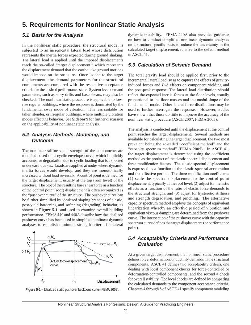
21Nonlinear Structural Analysis For Seismic Design: A Guide for Practicing Engineers
5. Requirements for Nonlinear Static Analysis 5.1 Basis for the Analysis
In the nonlinear static procedure, the structural model is subjected to an incremental lateral load whose distribution represents the inertia forces expected during ground shaking. The lateral load is applied until the imposed displacements reach the so-called “target displacement,” which represents the displacement demand that the earthquake ground motions would impose on the structure. Once loaded to the target displacement, the demand parameters for the structural components are compared with the respective acceptance criteria for the desired performance state. System level demand parameters, such as story drifts and base shears, may also be checked. The nonlinear static procedure is applicable to low-rise regular buildings, where the response is dominated by the fundamental sway mode of vibration. It is less suitable for taller, slender, or irregular buildings, where multiple vibration modes affect the behavior. See Sidebar 9 for further discussion on the applicability of nonlinear static analysis.
5.2 Analysis Methods, Modeling, and Outcome
The nonlinear stiffness and strength of the components are modeled based on a cyclic envelope curve, which implicitly accounts for degradation due to cyclic loading that is expected under earthquakes. Loads are applied at nodes where dynamic inertia forces would develop, and they are monotonically increased without load reversals. A control point is defined for the target displacement, usually at the top (roof level) of the structure. The plot of the resulting base shear force as a function of the control point (roof) displacement is often recognized as the “pushover curve” of the structure. The pushover curve can be further simplified by idealized sloping branches of elastic, post-yield hardening and softening (degrading) behavior, as shown in Figure 5-1, and used to examine overall building performance. FEMA 440 and 440A describe how the idealized pushover curve has been used in simplfied nonlinear dynamic analyses to establish minimum strength criteria for lateral
dynamic instability. FEMA 440A also provides guidance on how to conduct simplified nonlinear dynamic analyses on a structure-specific basis to reduce the uncertainty in the calculated target displacement, relative to the default method in ASCE 41.
5.3 Calculation of Seismic Demand
The total gravity load should be applied first, prior to the incremental lateral load, so as to capture the effects of gravity-induced forces and P-∆ effects on component yielding and the post-peak response. The lateral load distribution should reflect the expected inertia forces at the floor levels, usually proportional to the floor masses and the modal shape of the fundamental mode. Other lateral force distributions may be used to further interrogate the response. However, studies have shown that those do little to improve the accuracy of the nonlinear static procedure (ASCE 2007; FEMA 2005).
The analysis is conducted until the displacement at the control point reaches the target displacement. Several methods are available for calculating the target displacement, the two most prevalent being the so-called “coefficient method” and the “capacity spectrum method” (FEMA 2005). In ASCE 41, the target displacement is determined using the coefficient method as the product of the elastic spectral displacement and three modification factors. The elastic spectral displacement is expressed as a function of the elastic spectral acceleration and the effective period. The three modification coefficients (1) scale the spectral displacement to the control point displacement, typically at the roof level, (2) adjust for inelastic effects as a function of the ratio of elastic force demands to the structural strength, and (3) adjust for hysteretic stiffness and strength degradation, and pinching. The alternative capacity spectrum method employs the concepts of equivalent linearization whereby an effective period of vibration and equivalent viscous damping are determined from the pushover curve. The intersection of the pushover curve with the capacity spectrum curve defines the target displacement (or performance point).
5.4 Acceptability Criteria and Performance Evaluation
At a given target displacement, the nonlinear static procedure defines force, deformation, or ductility demands in the structural components. ASCE 41 defines two acceptability criteria, one dealing with local component checks for force-controlled or deformation-controlled components, and the second a check for overall stability. The local checks are defined by comparing the calculated demands to the component acceptance criteria. Chapters 4 through 8 of ASCE 41 specify component modeling Figure 5-1 – Idealized static pushover backbone curve (FEMA 2005).
Nonlinear Structural Analysis For Seismic Design: A Guide for Practicing Engineers
22
Sidebar 9Nonlinear Static Versus Nonlinear Dynamic Analysis
Nonlinear dynamic analysis methods generally provide more realistic models of structural response to strong ground shaking and, thereby, provide more reliable assessment of earthquake performance than nonlinear static analysis. Nonlinear static analysis is limited in its ability to capture transient dynamic behavior with cyclic loading and degradation. Nevertheless, the nonlinear static procedure provides a convenient and fairly reliable method for structures whose dynamic response is governed by first-mode sway motions. One way to check this is by comparing the deformed geometry from a pushover analysis to the elastic first-mode vibration shape. In general, the nonlinear static procedure works well for low-rise buildings (less than about five stories) with symmetrical regular configurations. FEMA 440, FEMA 440A, and NIST (2010) provide further details on the simplifying assumptions and limitations on nonlinear static analysis. However, even when the nonlinear static procedure is not appropriate for a complete performance evaluation, nonlinear static analysis can be an effective design tool to investigate aspects of the analysis model and the nonlinear response that are difficult to do by nonlinear dynamic analysis. For example, nonlinear static analysis can be useful to (1) check and debug the nonlinear analysis model, (2) augment understanding of the yielding mechanisms and deformation demands, and (3) investigate alternative design parameters and how variations in the component properties may affect response.
parameters and acceptance criteria for foundations, frames, walls, diaphragms, and other structural components made of steel, concrete, wood, and masonry. The strength criteria in ASCE 41 often refer to the underlying industry design standards for detailed information on material properties and the calculation of component strengths. The global dynamic instability check limits the magnitude of the inelastic strength reduction factor, reflecting the influence of P-∆ effects and post-peak negative stiffness in the structural components (Figure 5-1). The dynamic instability criterion of ASCE 41 is the same as one developed in FEMA 440. More recently, a revised dynamic instability criterion has been proposed in FEMA 440A, which is more accurate and less conservative than the limit in ASCE 41 and FEMA 440.
23Nonlinear Structural Analysis For Seismic Design: A Guide for Practicing Engineers
6. Requirements for Nonlinear Dynamics Analysis 6.1 Basis, Limitations, and Outcome for Nonlinear Dynamic Analysis
In contrast to the nonlinear static procedure, the nonlinear dynamic procedure, when properly implemented, provides a more accurate calculation of the structural response to strong ground shaking. Since the nonlinear dynamic analysis model incorporates inelastic member behavior under cyclic earthquake ground motions, the nonlinear dynamic procedure explicitly simulates hysteretic energy dissipation in the nonlinear range. Only the damping in the linear range and other non-modeled energy dissipation need to be added as viscous damping. The dynamic response is calculated for input earthquake ground motions, resulting in response history data on the pertinent demand parameters. Due to the inherent variability in earthquake ground motions, dynamic analyses for multiple ground motions are necessary to calculate statistically robust values of the demand parameters for a given ground motion intensity or earthquake scenario.
As nonlinear dynamic analysis involves fewer assumptions than the nonlinear static procedure, it is subject to fewer limitations than nonlinear static procedure. However, the accuracy of the results depends on the details of the analysis model and how faithfully it captures the significant behavioral effects. Acceptance criteria typically limit the maximum structural component deformations to values where degradation is controlled and the nonlinear dynamic analysis models are reliable.
6.2 Modeling of Inertial Mass and Gravity Load
The inertial mass should be the expected mass, including self weight of the building plus some allowance for contents, generally following the same assumptions as applied to determine seismic masses for design per ASCE 7 or other standards. It is usually adequate to lump the masses at the floor levels and to include inertial effects in the two horizontal directions, including rotation about the vertical building axis. Vertical inertial effects (i.e., vertical mass and ground motion components) should be modeled for buildings with long-span framing, e.g., arena roofs or long-span floor systems, where the vertical period of vibration is in the range that may be excited by the vertical component of earthquake ground motions (periods on the order of 0.1 seconds or larger). Otherwise, where members are sensitive to vertical loads, the influence of the code-specified vertical earthquake load, e.g., the Ev factor in ASCE 7, should be accounted for in the calculated force demands.
Gravity loads (defined and factored per ASCE 7) should be included in the dynamic analyses, so as to account for their
effects on (1) force and deformation demands in structural components and (2) large displacement P-∆ effects. Generally, inclusion of gravity loads will require a two-step (non-proportional loading) analysis, whereby the gravity loads are applied first and then held constant while the earthquake ground motions are applied.
6.3 Modeling of Damping Effects
In the context of the nonlinear dynamic procedure, equivalent viscous damping is associated with the reduction in vibrations through energy dissipation other than that which is calculated directly by the nonlinear hysteresis in the modeled elements. This so-called inherent damping occurs principally in (1) structural components that are treated as elastic but where small inelastic cracking or yielding occurs, (2) the architectural cladding, partitions, and finishes, and (3) the foundation and soil (if these are not modeled otherwise). Special energy dissipation components (e.g., viscous, friction, or hysteretic devices) should be modeled explicitly in the analysis, rather than as inherent damping.
The amount of inherent viscous damping requires careful consideration of the available sources of energy dissipation and whether these are otherwise captured in the analysis. For example, fiber-type component models, which capture the initiation and spread of yielding through the cross section and along the member lengths, will tend to capture hysteretic energy dissipation at lower deformations than lumped plasticity (hinge) models, where the inelastic hysteresis does not initiate until the demand exceeds the modeled yield strength of the member. Damping may also occur in components of the gravity framing that undergo local inelastic deformations but are not modeled directly in the structural analysis.
The equivalent viscous damping is included through the [C] term in the equation of motion. Two key questions are (1) what is an appropriate value for the inherent damping, and (2) how can the terms of the damping matrix be formulated to achieve that value. In the commonly employed Rayleigh damping formulation, the damping matrix [C] is calculated as a linear combination of the mass and stiffness matrix ([C]=am[M]+ak[K]), where the proportionality factors am and ak can be chosen to provide a defined percentage of critical damping at two specific periods of vibration. Reasonable periods to specify these damping values are 0.2T and 1.5T, where T is the fundamental period of vibration of the structure. In modal damping formulations, the damping matrix is formulated by specifying values of critical damping for one or more vibration modes, using information about the mode shapes and vibration periods. Alternatively, the damping effects of specific components, such as partition walls, could be modeled with explicitly defined viscous damping terms in the [C] matrix or hysteretic springs in the stiffness [K] matrix.
Nonlinear Structural Analysis For Seismic Design: A Guide for Practicing Engineers
24
specified damping to values within these ranges, it is further recommended to assess the sensitivity of the calculated demand parameters to the damping model formulation (e.g., Rayleigh versus modal) and the assumed critical damping values.
6.4 Input Ground Motions
Input ground motions should be selected and scaled so as to accurately represent the specific hazard of interest. As outlined in ASCE 7, the ground motions should reflect the characteristics of the dominant earthquake source at the building site, such as fault mechanism, distance to the fault, site conditions, and characteristic earthquake magnitude. Recent studies have further shown that the shape of the ground motion response spectra is an important factor in choosing and scaling ground motions, particularly for higher intensity motions (Baker and Cornell 2006). While a comprehensive discussion on the selection and scaling of ground motion records is beyond the scope of this Technical Brief, the following are some of the issues to consider:
Target hazard spectra or scenario: While the earthquake hazard is a continuum, building codes typically define specific ground motion hazard levels for specific performance checks. Generally, the hazard is defined in terms of response spectral accelerations with a specified mean annual frequency of exceedence, although other definitions are possible including scenario earthquakes, e.g., an earthquake with a specified magnitude and distance from the site, or deterministic bounds on ground motion intensities.
Source of ground motions: For building assessment and design, the input earthquake ground motions can either be (1) actual recorded ground motions from past earthquakes, (2) spectrally matched ground motions that are created by manipulating the frequency content and intensity of recorded ground motions to match a specific hazard spectrum, or (3) artificially simulated motions. Opinions differ as to which types are most appropriate. Recorded ground motions are generally scaled to match the hazard spectrum at one or more periods. For example, ASCE 7 specifies rules for scaling the ground motions based on their spectral acceleration values for periods between 0.2T to 1.5T, where T is the fundamental period of vibration of the structure. When structures are expected to respond in multiple modes, such as in tall buildings, spectral matching may be more appropriate, since scaling of actual recorded motions to a uniform hazard spectrum may bias the analysis results to either overestimate the response at short periods or underestimate it at longer periods. Number of ground motions: Given the inherent variability in earthquake ground motions, design standards typically require analyses for multiple ground motions to provide statistically robust measures of the demands. For example, ASCE 7 requires analyses for at least seven ground motions
The common Rayleigh and modal damping formulations were originally developed in the context of linear-elastic dynamic analysis, where the stiffness matrix [K] is constant and the vibration modes can be uniquely calculated. However, for nonlinear analysis, where member stiffnesses are changing and unique vibration modes do not exist, the application of each method has implementation issues, which are discussed by Hall (2006), Charney (2008), PEER/ATC 72-1, and others. For example, it is generally accepted that the stiffness proportional term of the damping matrix (ak[K]) should exclude or minimize contributions from components whose stiffness changes dramatically during the analysis or for components, such as rigid links, that are assigned artificially high stiffness. Some contend that this concern can be minimized by using the tangent rather than initial elastic stiffness matrix in the stiffness proportional damping term, while another suggested approach is to eliminate the stiffness proportional damping term and to only specify a value for the mass proportional damping term (am[M]). At present there is no clear consensus as to how to resolve these issues; moreover, some of the proposed solutions must be implemented within the software formulation and cannot otherwise be controlled by the software user. Therefore, the software documentation should be consulted for details on the damping implementation and guidance on specifying damping parameters.
The inherent damping depends on many factors specific to a given building, e.g., structural materials, type and detailing of partition and façade walls, height of building, foundation type, and the analysis model (e.g., lumped plasticity versus fiber type models). Therefore it is difficult to generalize as to the appropriate amount of additional damping to use in a nonlinear analysis. As summarized in PEER/ATC 72-1 measurements of total damping, expressed in terms of percent critical damping in the first translational mode, range from low values of 0.5 % to 1 % in buildings under wind and ambient vibrations up to 10 % in buildings subjected to earthquakes. However, in the latter case, the measured damping of 10 % is likely to reflect energy dissipation due to both nonlinear hysteretic and inherent damping. Thus, reported measurements of damping require careful interpretation.
Based on these observations and guidance in various documents, it is suggested to specify equivalent viscous damping in the range of 1 % to 5 % of critical damping over the range of elastic periods from 0.2T to 1.5T (with T as defined previously). Critical damping values should be specified in the lower end of this range for (1) tall buildings and other structures where there is less participation by partition walls, cladding and foundations, and (2) service level earthquake analyses where story drift ratios are limited to about 0.005. For tall buildings, the Pacific Earthquake Engineering Research Center guidelines (PEER 2010) recommend that viscous damping be less than 2.5% over the range of predominant modes, and Council on Tall Buildings and the Urban Habitat (Willford et al. 2008) recommends damping values in the range of 1% to 2%. Beyond limiting the
•
•
•
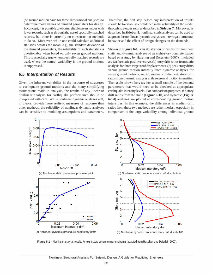
25Nonlinear Structural Analysis For Seismic Design: A Guide for Practicing Engineers
(or ground motion pairs for three-dimensional analyses) to determine mean values of demand parameters for design. In concept, it is possible to obtain reliable mean values with fewer records, such as through the use of spectrally matched records, but there is currently no consensus on methods to do so. Moreover, while one could calculate additional statistics besides the mean, e.g., the standard deviation of the demand parameters, the reliability of such statistics is questionable when based on only seven ground motions. This is especially true when spectrally matched records are used, where the natural variability in the ground motions is suppressed.
6.5 Interpretation of Results
Given the inherent variability in the response of structures to earthquake ground motions and the many simplifying assumptions made in analysis, the results of any linear or nonlinear analysis for earthquake performance should be interpreted with care. While nonlinear dynamic analyses will, in theory, provide more realistic measures of response than other methods, the reliability of nonlinear dynamic analyses can be sensitive to modeling assumptions and parameters.
Therefore, the first step before any interpretation of results should be to establish confidence in the reliability of the model through strategies such as described in Sidebar 7. Moreover, as described in Sidebar 9, nonlinear static analyses can be used to augment the nonlinear dynamic analysis to interrogate structural behavior and the effect of design changes on the demands.
Shown in Figure 6-1 is an illustration of results for nonlinear static and dynamic analyses of an eight-story concrete frame, based on a study by Haselton and Deierlein (2007). Included are (a) the static pushover curve, (b) story drift ratios from static analysis for three target roof displacements, (c) peak story drifts versus ground motion intensity from dynamic analyses for seven ground motions, and (d) medians of the peak story drift ratios from dynamic analyses at three ground motion intensities. The results shown here are just a small sample of the demand parameters that would need to be checked at appropriate earthquake intensity levels. For comparison purposes, the story drift ratios from the static (Figure 6-1b) and dynamic (Figure 6-1d) analyses are plotted at corresponding ground motion intensities. In this example, the differences in median drift ratios from these two methods are rather modest, especially in comparison to the large variability among individual ground
Figure 6-1 – Nonlinear analysis results for eight story concrete moment frame (adapted from Haselton and Deierlein 2007).
(b) Nonlinear static procedure story drift distribution(a) Nonlinear static procedure pushover plot
(d) Nonlinear dynamic procedure story drift distribution(c) Nonlinear dynamic procedure peak story drifts
Nonlinear Structural Analysis For Seismic Design: A Guide for Practicing Engineers
26
motions (Figure 6-1c). NIST (2010) conducted a more detailed study of the relative accuracy between nonlinear static and dynamic analyses.
According to ASCE 7 and as commonly applied in practice, when seven or more ground motions are run, the calculated mean demand parameter values should be compared to the acceptance criteria for the specified performance levels. Assuming a lognormal distribution of demand parameters with a dispersion (standard deviation of the natural log of the data and similar to a coefficient of variation) of 0.5, the checks based on mean values imply that the acceptance criteria would be exceeded about 40 % of the time. This large probability of exceedence is an accepted standard of practice, provided that the likelihood (e.g., mean annual frequency of exceedence) of the specified earthquake intensity is sufficiently low for the performance level being checked. However, where “overload” of non-ductile force-controlled components may lead to sudden failures that could significantly affect the overall building safety, it is generally recognized that more stringent criteria should be applied.
The PEER Seismic Design Guidelines for Tall Buildings (2010) specify required strengths for force-controlled elements equal to 1.3 to 1.5 times the mean demand parameter, where the lower multiplier (1.3) is permitted for systems where capacity design is used to shield force-controlled members. Assuming dispersion of 0.5 in the displacement demands, there is a 15 % to 20 % probability that the actual demands will exceed the specified required strengths, i.e., 1.3 to 1.5 times the calculated mean demands. Whether or not these increased deformation demands will translate into increased component force demands depends on the structural configuration and the interaction of yielding and non-yielding components. While relatively straightforward to apply, the simple demand multipliers assume a fixed relationship between ground motion intensities, drifts, and component deformation and force demands. This assumption is very approximate for nonlinear systems. An alternative method to evaluate the increased demands is to (1) repeat the nonlinear dynamic analyses for ground motions whose intensities are factored up by an appropriate factor (e.g., a factor of 1.5 based on the PEER guidelines), and (2) calculate mean demands for critical force-controlled components under the amplified input motions. This alternative procedure has the benefit of accounting directly for inelastic force redistributions and possible shielding of force-controlled components. While both of these approaches account for variability in earthquake ground motions, neither directly addresses structural model uncertainties, where the variation in response of specific structural components may change the inelastic mechanisms and distribution of internal forces and deformations. Therefore, where the uncertainty in analysis model parameters is large and has the potential to significantly alter the structural response, it may be appropriate to interrogate the model for such effects. This could be done by systematically varying the model properties for the critical components and conducting dynamic
and/or static nonlinear analyses to characterize the change in the calculated demand parameters.
In spite of the large inherent uncertainties in earthquake ground motions and their effects on structures, nonlinear dynamic analysis is considered to be the most reliable method available to evaluate the earthquake performance of buildings. Primarily, the nonlinear dynamic procedure enables the evaluation of design decisions on a more consistent and rational basis as compared to other simplified analysis methods. The potential impact of uncertainties in the structural response can, to some extent, be mitigated through capacity design approaches in new buildings and to some extent in devising structural retrofits for existing buildings. Otherwise, the uncertainties can be addressed using the methods suggested previously. Ultimately, the engineer must understand the capabilities and limitations of any method of analysis and make appropriate use of it to characterize the structural behavior with sufficient accuracy and confidence for design.
27Nonlinear Structural Analysis For Seismic Design: A Guide for Practicing Engineers
ACI (2008). Building code requirements for structural concrete (ACI 318-08) and commentary (ACI 318R-08), American Concrete Institute, Farmington Hills, MI.
AISC (2010). Seismic provisions for structural steel buildings, ANSI/AISC 341-10, American Institute of Steel Construction, Chicago, IL.
ASCE (2007). Seismic rehabilitation of existing buildings, ASCE/SEI Standard 41-06 with supplement 1, American Society of Civil Engineers, Reston, VA.
ASCE (2010). Minimum design loads for buildings and other structures, ASCE/SEI Standard ASCE 7-10, American Society of Civil Engineers, Reston, VA.
ATC (1996). Seismic evaluation and retrofit of concrete buildings, ATC 40, Applied Technology Council, Redwood City, CA.
ATC (2009). Guidelines for seismic performance assessment of buildings, ATC 58, 50 % Draft Report, Applied Technology Council, Redwood City, CA.
Baker, J. W. and Cornell, C. A. (2006). “Spectral shape, epsilon and record selection,” Earthquake Engineering and Structural Dynamics, 35 (9), p. 1077-1095.
Charney, F. A. (2008). “Unintended consequences of modeling damping in structures,” Journal of Structural Engineering, American Society of Civil Engineers, 134 (4), p. 581-592.
Charney, F. A. and Marshall, J. D. (2006). “A comparison of the Krawinkler and scissors models for including beam-column joint deformations in the analysis of moment-resisting steel frames,” Engineering Journal, American Institute of Steel Construction, 43 (1), p. 31-48.
Charney, F. A. and McNamara, R. J. (2008). “A method for computing equivalent viscous damping ratio for structures with added viscous damping,” Journal of Structural Engineering, American Society of Civil Engineers, 134 (1), p. 32-44.
Constantinou, M. C. and Symans, M. D. (1993). “Seismic response of structures with supplemental damping,” Structural Design of Tall Buildings, 2 (2), p. 77-92.
Constantinou, M. C., Soong, T. T., and Dargush, G. F. (1998). Passive energy dissipation for structural design and retrofit, Multidisciplinary Center for Earthquake Engineering Research Monograph Series, University at Buffalo, Buffalo, NY.
Constantinou, M. C., Reinhorn, A. M., Tsopelas, P., and Nagarajaiah, S. (1999). “Techniques in the nonlinear dynamic analysis of seismic isolated structures,” Structural Dynamic Systems Computational Techniques and Optimization: Seismic Techniques, Gordon and Breach International Series in Engineering Technology and Applied Science, Vol. 12, p. 1-24, Gordon and Breach Science Publishers, Amsterdam, The Netherlands.
Fell, B. V., Kanvinde, A., and Deierlein, G. G. (2010). Large-scale testing and simulation of earthquake induced ultra low cycle fatigue in bracing members subjected to cyclic inelastic buckling, Blume Earthquake Engineering Center TR 172, Stanford University, Stanford, CA.
FEMA (1997). NEHRP guidelines for the seismic rehabilitation of buildings, FEMA Report 273, Washington, D.C. FEMA (2002). Earthquake loss estimation methodology, HAZUS99-SR2, advanced engineering building module, technical and user’s manual. Federal Emergency Management Agency, Washington, D.C.
FEMA (2005). Improvement of nonlinear static seismic analysis procedures, FEMA Report 440, Washington, D.C.
7. References
Nonlinear Structural Analysis For Seismic Design: A Guide for Practicing Engineers
28
FEMA (2006). HAZUS-MH MR2 Multi-hazard loss estimation methodology, earthquake model, technical manual. Federal Emergency Management Agency, Washington, D.C.
FEMA (2009a). Effects of strength and stiffness degradation on the seismic response of structural systems, FEMA Report 440a, Washington, D.C.
FEMA (2009b). Evaluation of earthquake damaged concrete and masonry wall buildings, FEMA Report 306, Washington, D.C.
Ghobarah, A. and Biddah, A. (1999). “Dynamic analysis of reinforced concrete frames including joint shear deformation,” Engineering Structures, 21 (11), p. 971-987.
Hall, J. F. (2006). “Problems encountered from the use (or misuse) of Rayleigh damping,” Earthquake Engineering and Structural Dynamics, 35 (5), p. 525-545.
Hamburger, R. O., Krawinkler, H. K., Malley, J. O., and Adan, S. M. (2009). Seismic design of special moment frames: A guide for practicing engineers, NEHRP Seismic Design Technical Brief No. 2., NIST GCR 09-917-3, National Institute of Standards and Technology, Gaithersburg, MD.
Haselton, C. B. and Deierlein, G. G. (2007). Assessing seismic collapse safety of modern reinforced concrete moment frame buildings, Blume Earthquake Engineering Center TR 156, Stanford University, Stanford, CA.
Ibarra, L., Medina, R., and Krawinkler, H. (2005). “Hysteretic models that incorporate strength and stiffness deterioration,” Earthquake Engineering and Structural Dynamics, 34 (12), p. 1489-1511.
Kadysiewski, S. and Mosalam, K. M. (2009). Modeling of unreinforced masonry infill walls considering in-plane and out-of-plane interaction, PEER Report 2008/102, Pacific Earthquake Engineering Research Center, University of California at Berkeley, Berkeley, CA.
Kircher, C. A., Nassar, A. A., Kustu, O., and Holmes, W. T. (1997a). “Development of Building Damage Functions for Earthquake Loss Estimation,” Earthquake Spectra, 13 (4), p. 663-682.
Kircher, C. A., Reitherman, R. K., Whitman, R. V., and Arnold, C. (1997b). “Estimation of Earthquake Losses to Buildings,” Earthquake Spectra, 13 (4), p. 703-720.
Kunnath, S. K., Reinhorn, A. M. and Park, Y. J. (1990). “Analytical modeling of inelastic seismic response of R/C structures,” Journal of Structural Engineering, American Society of Civil Engineers, 116 (4), p. 996-1017.
Lowes, L. N. and Altoontash, A. (2003). “Modeling reinforced concrete beam-column joints subjected to cyclic loading,” Journal of Structural Engineering, American Society of Civil Engineers, 129 (12), p. 1686-1697.
Madan, A., Reinhorn, A. M., Mander, J., and Valles, R. (1997). “Modeling of Masonry Infill Panels For Structural Analysis,” Journal of Structural Engineering, American Society of Civil Engineers, 123 (10), p. 1295-1302.
Moehle, J. P., Hooper, J. D., and Lubke, C. D. (2008). Seismic design of reinforced concrete special moment frames: A guide for practicing engineers, NEHRP Seismic Design Technical Brief No. 1., NIST GCR 09-917-1, National Institute of Standards and Technology, Gaithersburg, MD.
Moehle, J. P., Hooper, J. D., Kelly, D. J., and Meyer T. R. (2010). Seismic design of cast-in-place concrete diaphragms, chords, and collectors, NEHRP Seismic Design Technical Brief No. 3., NIST GCR 10-917-4, National Institute of Standards and Technology, Gaithersburg, MD.
Nagarajaiah, S., Reinhorn, A. M., and Constantinou, M. C. (1991). “Nonlinear dynamic analysis of three dimensional base isolated structures,” Journal of Structural Engineering, American Society of Civil Engineers, 117 (7), p. 2035-2054.
29Nonlinear Structural Analysis For Seismic Design: A Guide for Practicing Engineers
Naeim, F. and Kelly, J. M. (1999). Design of seismic isolated structures: From theory to practice, John Wiley and Sons, Inc., New York, NY.
NIST (2010). Applicability of nonlinear multiple-degree-of-freedom modeling for design, NIST GCR 10-917-9, prepared by the NEHRP Consultants Joint Venture for the National Institute of Standards and Technology, Gaithersburg, MD. Paulay, T. and Priestley, M. J. N. (1992). Seismic design of reinforced concrete and masonry buildings, John Wiley and Sons, Inc., New York, NY.
PEER (2010). Seismic design guidelines for tall buildings, Pacific Earthquake Engineering Research Center, University of California at Berkeley, Berkeley, CA.
PEER/ATC (2010). Modeling and acceptance criteria for seismic design and analysis of tall buildings, PEER/ATC 72-1 Report, Applied Technology Council, Redwood City, CA, October 2010.
Powell, G. (2010). Modeling for structural analysis – Behavior and basics, Computers and Structures, Inc., Berkeley, CA (in press).
Reinhorn, A. M., Roh, H., Sivaselvan, M., Kunnath, S. K., Valles, R. E., Madan, A., Li, C., Lobo, R., and Park, Y. J. (2009). IDARC 2D Version 7.0: A program for the inelastic damage analysis of structures, Technical Report MCEER-09-0006, University at Buffalo, State University of New York.
Schachter, M. and Reinhorn, A. M. (2007). Three-dimensional modeling of inelastic buckling in frame structures, Technical Report MCEER-07-0016, University at Buffalo, State University of New York.
Spacone, E., Filippou, F. C., and Taucer, F. F. (1996). “Fiber beam-column model for nonlinear analysis of R/C frames. 1: formulation,” Earthquake Engineering and Structural Dynamics, 25 (7), p. 711-725.
Tang, X. and Goel, S. C. (1989). “Brace fractures and analysis of phase I structures,” Journal of Structural Engineering, American Society of Civil Engineers, 115 (8), p. 1960-1976.
Uriz, P. and Mahin, S. A. (2008). Towards earthquake resistant design of concentrically braced steel structures, PEER 2008/08, Pacific Earthquake Engineering Research Center, University of California at Berkeley, Berkeley, CA.
Willford, M., Whittaker, A., and Klemencic, R. (2008). Recommendations for the seismic design of high-rise buildings, Council on Tall Buildings and Urban Habitat, Illinois Institute of Technology, Chicago, IL.
Wilson, E. (2002). Three-dimensional static and dynamic analysis of structures, 3rd Ed., Computers and Structures Inc., Berkeley, CA.
Werkle, H. and Waas, G. (1986). “Dynamic stiffness of foundations on inhomogeneous soils,” Proceedings of the 8th European Conference on Earthquake Engineering, Lisbon, Portugal.
Wolf, J. P. (1985). Dynamic soil-structure interaction, Prentice Hall, Englewood Cliffs, NJ.
Nonlinear Structural Analysis For Seismic Design: A Guide for Practicing Engineers
30
8. Notations and Abbreviations

31Nonlinear Structural Analysis For Seismic Design: A Guide for Practicing Engineers
Abbreviations
ACI American Concrete Institute
AISC American Institute of Steel Construction
ASCE American Society of Civil Engineers
ATC Applied Technology Council
CUREE Consortium of Universities for Research in Earthquake Engineering
FEMA Federal Emergency Management Agency
NIST National Institute of Standards and Technology
SEI Structural Engineering Institute
PEER Pacific Earthquake Engineering Research Center
NEHRP National Earthquake Hazards Reduction Program
Nonlinear Structural Analysis For Seismic Design: A Guide for Practicing Engineers
32
9. CreditsCover photo Image courtesy of Tipping Mar
Figure 1-1 (a) Image courtesy of KMD Architects and Tipping Mar
Figure 1-1 (b) Image courtesy of Tipping Mar
Figure 2-1 Image courtesy of Kevin Wong and Andrei Reinhorn
Figure 2-2 Image courtesy of Kevin Wong and Andrei Reinhorn
Figure 2-3 Image courtesy of Kevin Wong and Andrei Reinhorn
Figure 2-4 Image courtesy of American Society of Civil Engineers Printed with permission from ASCE
Figure 2-5 Image courtesy of Applied Technology Council
Figure 2-6 Image courtesy of Federal Emergency Management Agency
Figure 2-7 Image courtesy of Applied Technology Council
Figure 2-8 Image courtesy of Kevin Wong and Andrei Reinhorn
Figure 3-1 Image courtesy of Greg Deierlein
Figure 3-2 Image courtesy of Benjamin Fell
Figure 3-3 Image courtesy of Kevin Wong and Andrei Reinhorn
Figure 3-4 Image courtesy of Applied Technology Council
Figure 3-5 Image courtesy of Kevin Wong and Andrei Reinhorn
Figure 4-1 Image courtesy of Kevin Wong and Michael Willford
Figure 4-2 Image courtesy of Kevin Wong and Michael Willford
Figure 5-1 Image courtesy of Federal Emergency Management Agency
Figure 6-1 Image courtesy of Curt Haselton and Greg Deierlein