Nonlinear State EstimationParticle, Sigma-Points Filters

Robert Stengel Optimal Control and Estimation, MAE 546

Princeton University, 2018

Copyright 2018 by Robert Stengel. All rights reserved. For educational use only.http://www.princeton.edu/~stengel/MAE546.html

http://www.princeton.edu/~stengel/OptConEst.html

!  Particle filter!  Sigma-Points (“Unscented

Kalman”) filter!  Transformation of uncertainty!  Propagation of mean and

variance!  Helicopter, HIV state

estimation examples!  Additional nonlinear filters

1

Criticisms of the Basic Extended Kalman Filter*

*Julier and Uhlmann, 1997; Wan and van der Merwe, 2001

•  State estimate prediction is deterministic, i.e., not based on an expectation –  (Not true; the state estimate is the expectation of the

mean)•  State estimate update is linear (unless it is quasi-

linear, iterated, or adapted)•  Jacobians must be evaluated to calculate

covariance prediction and update

2

Transformation of Uncertainty

The transformation is said to be “unscented”*if its probability distribution is

Consistent, Efficient, and Unbiased

Estimate of the mean and covariance of the transformation’s output

y = f x[ ]where

x is a random variable with mean, x, and covariance, Pxx

y x,Pxx( ) and Pyy x,Pxx( )

Nonlinear transformation of a random variable

Julier and Uhlmann, 1997 3

Consistent Estimate of a Dynamic State

Consistent state estimate converges in the limitPxk+1xk+1

−E xk+1 − xk+1( ) xk+1 − xk+1( )T⎡⎣

⎤⎦{ }≥ 0

Estimated Covariance – Actual Covariance{ }≥ 0

Let xk ! x, xk+1 ! y

Lesson: In filtering, add sufficient “process noise” to the filter gain computation to

prevent filter divergence

xk+1 xk ,Pxkxk( ) = y x,Pxx( )

Pxk+1xk+1 xk ,Pxkxk( ) = Pyy x,Pxx( )

4

Adding Process Noise Improves

Consistency•  Satellite orbit

determination–  Aerodynamic drag

produced unmodeled bias

–  Optimal filter did not estimate bias

•  Process noise increased for filter design–  Divergence is contained

Fitzgerald, 1971 5

Filter’s estimate of RMS state error

Actual state estimate error

Filter’s estimate of RMS state error

Actual state estimate error

Efficient and Unbiased Estimate of a Dynamic State

minAdded Process Noise

Estimated Covariance – Actual Covariance{ }

xk+1 = E xk+1( )Estimated Mean = Actual Mean

Efficient state estimator converges more quickly than an inefficient estimator

Unbiased estimate

Add “just enough” process noise

6

Empirical Determination of a Probability Distribution

!  Monte Carlo evaluation!  Propagate random noise through nonlinearity

for given prior distribution (e.g., Gaussian)!  Generate histogram of output

!  N trials) of nonlinear system propagation!  Histogram as numerical representation of distribution,

or!  Functional minimization to identify associated

theoretical distribution

7

!  Particle Filter !  Propagate many points to estimate mean and

standard deviation!  As N –> ∞, estimate error –> 0

x =xi

i=1

N

∑N

!  Sample variance for same data set σ x

2 =xi − x( )2

i=1

N

∑N −1( )

!  Sample mean for N data points, x1, x2, ..., xN

Empirical Determination of Mean and Variance

8

!  Sigma Points Filter: !  Propagate limited number of points

using nonlinear model to estimate mean and covariance

Sigma Points of Pxx and Mean2-D Example

Elliptical One-Sigma Contour

9

!  Mean is center of ellipse!  Sigma points are ± major and

minor axes of ellipse

Sigma Points of Pxx and E(x)

3-D Example

10

!  Mean is center of ellipsoid!  Sigma points are ± extremes

of ellipsoid axes

Sigma Points of Estimate Uncertainty, Pxx

State covariance matrixPxx : Symmetric, positive-definite covariance matrix

Eigenvalues are real and positive

sIn − Pxx = s − λ1( ) s − λ2( ) s − λn( )Eigenvectors

λiIn − Pxx( )αei = 0, i = 1,n

11

Modal matrix (not expected value symbol)

E = e1 e2 ! en⎡

⎣⎤⎦

Sigma Points of PxxDiagonalized covariance matrixEigenvalues are the Variances

1)  Principal axes of the covariance matrix are defined by modal matrix, E

2)  Location of 2n one-sigma points in state space given by

±Δx σ1( ) ±Δx σ 2( ) ±Δx σ n( )⎡⎣⎢

⎤⎦⎥ = E

±σ1 0 00 ±σ 2 0 0 0 ±σ n

⎡

⎣

⎢⎢⎢⎢⎢

⎤

⎦

⎥⎥⎥⎥⎥

Λ = E−1PxxE = ETPxxE =

λ1 0 00 λ2 0 0 0 λn

⎡

⎣

⎢⎢⎢⎢⎢

⎤

⎦

⎥⎥⎥⎥⎥

=

σ12 0 0

0 σ 22 0

0 0 σ n

2

⎡

⎣

⎢⎢⎢⎢⎢

⎤

⎦

⎥⎥⎥⎥⎥

12

Propagation of the Mean Value and Covariance Matrix

13

Propagation of the Mean Value and the Sigma Points

!  Mean value at tk

!  Sigma points (relative to mean value)

σ ik!

xk −Δxk σ i( ), i =1,n

xk +Δxk σ i( ), i = n+1( ),2n

⎧⎨⎪

⎩⎪

x tk( ) = xk

xk+1 = xk + f x t( ), u t( ),w t( ),t⎡⎣ ⎤⎦dttk

tk+1

∫

σ ik+1 = σ ik + f σ i t( ), u t( ),w t( ),t⎡⎣ ⎤⎦dttk

tk+1

∫ , i =1,2n

Projection from the prior mean

Nonlinear projection from each prior sigma point

14

Estimation of the Propagated Mean Value

•  Assumptions:•  To 2nd order, the propagated probability distribution is

symmetric about its mean•  New mean is estimated as average or weighted average of

projected points (arbitrary choice by user)

xk+1 =xk+1 + σ ik+1

i=1

2n

∑2n +1

xk+1 =xk+1 + ξ σ ik+1

i=1

2n

∑2ξn +1

Ensemble Average for the Mean Value

Weighted Ensemble Average for the Mean Value

15

Projected Covariance Matrix

Pxk+1xk+1 =

12n +1( )−1 xk+1 − xk+1( ) xk+1 − xk+1( )T + σ ik+1

− xk+1( ) σ ik+1− xk+1( )T

i=1

2n

∑⎧⎨⎩

⎫⎬⎭

Unbiased ensemble estimate of the covariance matrix

This estimate neglects effects of disturbance uncertainty during the state propagation from tk to tk+1

16

Does not require calculation of Jacobian matricesDoes require calculation of nonlinear integrals

Sigma Points of Disturbance Uncertainty, Q

Q : s × s( ) Symmetric, positive-definite covariance matrix

sIs −Q = s − λ1( ) s − λ2( ) s − λs( ) [s = Laplace operator]

λiIs −Q( )αei = 0, i = 1, s

EQ = e1 e2 es⎡⎣

⎤⎦Q

ΛQ = EQTQEQ =

λ1 0 ! 00 λ2 ! 0! ! ! !0 0 ! λs

⎡

⎣

⎢⎢⎢⎢⎢

⎤

⎦

⎥⎥⎥⎥⎥Q

=

σ 12 0 ! 0

0 σ 22 ! 0

! ! ! !0 0 ! σ s

2

⎡

⎣

⎢⎢⎢⎢⎢

⎤

⎦

⎥⎥⎥⎥⎥Q

!  Eigenvalues!  Modal Matrix!  Transformation

17

±Δw σ 1( ) ±Δw σ 2( ) ! ±Δw σ s( )⎡⎣⎢

⎤⎦⎥ = EQ

±σ 1 0 ! 00 ±σ 2 ! 0! ! ! !0 0 ! ±σ s

⎡

⎣

⎢⎢⎢⎢⎢

⎤

⎦

⎥⎥⎥⎥⎥Q

Propagation of the Disturbed Mean Value

Sigma points of disturbance (relative to mean value)

ω ik

wk + Δwk σ i( ), i = 1, s

wk − Δwk σ i( ), i = s +1( ),2s⎧⎨⎪

⎩⎪

xω i( )k+1

= xk + f x t( ),u t( ),ω i t( ),t⎡⎣ ⎤⎦dttk

tk+1

∫ , i = 1,2s

Incorporation of effects of disturbance uncertainty on state propagation

18Calculation of nonlinear integrals

Estimation of the Propagated Mean Value with Disturbance Uncertainty

Estimate now includes effect of disturbance uncertaintyEstimate of the mean is the average or weighted average of

projected points

xk+1 =xk+1 + σ ik+1

i=1

2n

∑ + xω i( )k+1

i=1

2s

∑2 n + s( ) +1

xk+1 =xk+1 + ξ σ ik+1

i=1

2n

∑ + xω i( )k+1

i=1

2s

∑⎡⎣⎢

⎤⎦⎥

2ξ n + s( ) +1

Ensemble Average for the Mean Value

Weighted Ensemble Average for the Mean Value

19

Covariance Propagation with Disturbance Uncertainty

Pxk+1xk+1 =1

2 n + s( ) +1⎡⎣ ⎤⎦ −1Pmean + Psigma + Pdisturbance( )

Unbiased sampled estimate of the covariance matrix

Pmean = xk+1 − xk+1( ) xk+1 − xk+1( )T

Psigma = σ ik+1− xk+1( ) σ ik+1

− xk+1( )Ti=1

2n

∑

Pdisturbance = xω i( )k+1

− xk+1⎡⎣

⎤⎦ xω i( )

k+1− xk+1⎡

⎣⎤⎦T

i=1

2s

∑20

Sigma-Points (“Unscented Kalman”)

Filter

21

System Vector Notation

v xwn

⎡

⎣

⎢⎢⎢

⎤

⎦

⎥⎥⎥

dim v( ) = n + r + s( )×1

v0 =x0w0

n0

⎡

⎣

⎢⎢⎢

⎤

⎦

⎥⎥⎥= E

x0w0

n0

⎡

⎣

⎢⎢⎢

⎤

⎦

⎥⎥⎥ χ0 =

χ0x

χ0w

χ0n

⎡

⎣

⎢⎢⎢⎢

⎤

⎦

⎥⎥⎥⎥

χk+1x = χk

x + f χx t( ),u t( ),χw t( ),t⎡⎣ ⎤⎦dttk

tk+1

∫

ψ = h χx ,χn( )

System vector Expected value of system vector

Measurement vector, corrupted by noise

Propagation of the mean

Analogous to z t( ) = Hx t( ) + n t( )22

Matrix Array of System and Sigma-Point Vectors

Χ χ0 χ1 χ2L⎡

⎣⎤⎦; dim Χ( ) = L × 2L +1( )

χ0 = v0 =x0w0

n0

⎡

⎣

⎢⎢⎢

⎤

⎦

⎥⎥⎥; dim χ0( ) = n + r + s( )×1 L ×1

χi =v i + ξ S( )i , i = 1,L

v i −ξ S( )i , i = L +1,2L

⎧⎨⎪

⎩⎪

⎫⎬⎪

⎭⎪; dim χi( ) = 2L ×1

S : Square root of P; S( )i ith column of S

Weighted sigma points for system vector

Matrix of mean and sigma-point vectors

Expected value of system vector

23

Initialize FilterState and covariance estimates

xo = E x 0( )⎡⎣ ⎤⎦ = χx 0( )

Px 0( ) = E x 0( )− x 0( )⎡⎣ ⎤⎦ x 0( )− x 0( )⎡⎣ ⎤⎦T{ }

Pv 0( ) = E v 0( )− v 0( )⎡⎣ ⎤⎦ v 0( )− v 0( )⎡⎣ ⎤⎦T{ }

=

Px 0( ) 0 0

0 Qw 0( ) 0

0 0 Rn 0( )

⎡

⎣

⎢⎢⎢⎢

⎤

⎦

⎥⎥⎥⎥

Covariance matrix of system vector

24

Propagate State Mean and Covariance

xk+1 −( ) = ηi χixk+1

i=0

2L

∑

χix( )k+1 = χi

x( )k + f χix( ) t( ),u t( ), χi

w( ) t( ),t⎡⎣ ⎤⎦dttk

tk+1

∫

Incorporate disturbance sigma points

Ensemble average estimates of mean and covarianceηi : Weighting factor

Typically

ηi =1 L +1( ), i = 0

1 2 L +1( ), i = 1,2L

⎧⎨⎪

⎩⎪

25after Wan and van der Merwe, 2001

Pk+1x −( ) = ηi χi

x −( )− x −( )⎡⎣ ⎤⎦k+1 χix −( )− x −( )⎡⎣ ⎤⎦k+1

T{ }i=0

2L

∑

Incorporate Measurement Error in Output

ψ i( )k+1 = h χix( )k+1 , χi

n( )k+1⎡⎣ ⎤⎦, i = 0,2L

yk+1 −( ) = ηi ψ i k+1i=0

2L

∑

Mean/sigma-point projections of measurement

Weighted estimate of measurement projection

26

Incorporate Measurement Error in Covariance

Prior estimate of measurement covariance

Prior estimate of state/measurement cross-covariance

27after Wan and van der Merwe, 2001

Pk+1y −( ) = ηi ψ i −( )− y −( )⎡⎣ ⎤⎦k+1 ψ i −( )− y −( )⎡⎣ ⎤⎦k+1

T{ }i=0

2L

∑

Pk+1xy −( ) = ηi χi

x −( )− x −( )⎡⎣ ⎤⎦k+1 ψ i −( )− y −( )⎡⎣ ⎤⎦k+1T{ }

i=0

2L

∑

Compute Kalman Filter Gain

Kk+1 = Pk+1xy −( ) Pk+1y −( )⎡⎣ ⎤⎦

−1

Original formula (eq. 3, Lecture 18)

Kk = Pk −( )HkT HkPk −( )Hk

T + Rk⎡⎣ ⎤⎦−1

Sigma points version w/index change

28

Post-Measurement State and Covariance Estimate

xk+1 +( ) = xk+1 −( ) +Kk+1 zk+1 − yk+1 −( )⎡⎣ ⎤⎦

Pk+1x +( ) = Pk+1x −( ) −Kk+1Pk+1

y −( )Kk+1T

State estimate update

Covariance estimate “update”

29

30

Example: Simulated Helicopter UAV Flightvan der Werwe and Wan, 2004

Comparison of Pitch, Roll, and Yaw Errors

31

Comparison of RMS Errors for EKF, UKF, and Gauss-Hermite Filter (GHF)

32Banks et al, A COMPARISON OF NONLINEAR FILTERING APPROACHESIN THE CONTEXT OF AN HIV MODEL, 2010

CD4+ Cells

HIV Virions

Effector Cells

EKF UKF GHF

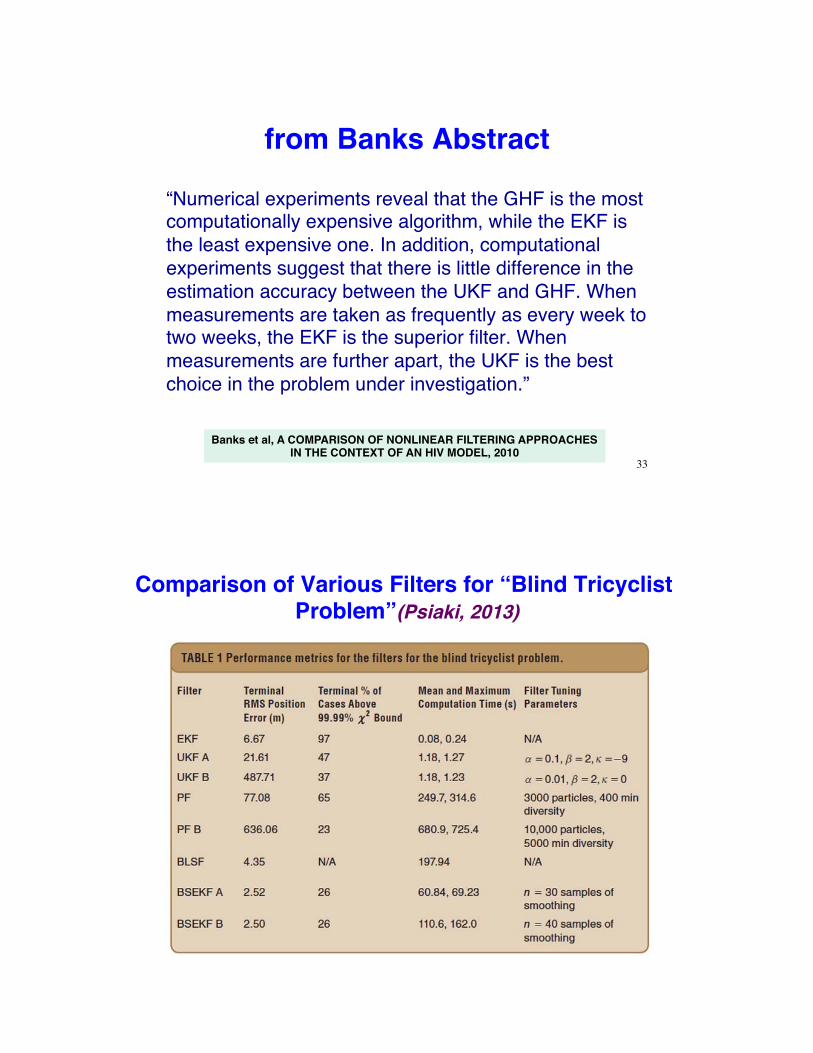
from Banks Abstract

“Numerical experiments reveal that the GHF is the most computationally expensive algorithm, while the EKF is the least expensive one. In addition, computational experiments suggest that there is little difference in the estimation accuracy between the UKF and GHF. When measurements are taken as frequently as every week to two weeks, the EKF is the superior filter. When measurements are further apart, the UKF is the best choice in the problem under investigation.”

33

Banks et al, A COMPARISON OF NONLINEAR FILTERING APPROACHESIN THE CONTEXT OF AN HIV MODEL, 2010

Comparison of Various Filters for “Blind Tricyclist Problem”(Psiaki, 2013)

34

Comparison of Various Filters for “Blind Tricyclist Problem”(Psiaki, 2013)

35

Definitions

36

!  EKF: Extended Kalman filter•  UKF: Unscented Kalman (Sigma-

Points) filter•  GHF: Gauss-Hermite filter*•  PF: Particle filter•  BLSF: Batch least-squares filter•  BSEKF: Backward-smoothing EKF

* See https://ieeexplore.ieee.org/stamp/stamp.jsp?arnumber=6838186 https://en.wikipedia.org/wiki/Gauss–Hermite_quadrature

Observations!  Jacobians vs. no Jacobians!  Number of nonlinear propagation steps!  Gaussian vs. approximate non-Gaussian

distributions!  Best choice of averaging weights is problem-

dependent!  Comparison of filters is problem-dependent

!  Are these filters better than a quasi-linear filter? (TBD)

37

More on Nonlinear Estimators!  Gordon, N., Salmond,D., and Smith, A. “Novel Approach to

Nonlinear/Non-Gaussian Bayesian State Estimation,” IEE Proc.-F, (140(2), Apr 1993, pp. 107-113.

!  Banks, H., Hu, S., Kenz, Z., and Tran, H., “A Comparison of Nonlinear Filtering Approaches in the Context of an HIV Model,” Math. Biosci. Eng., 7 (2), Apr 2010, pp. 213-236.

!  Psiaki, M., “Backward-Smoothing Extended Kalman Filter,” Journal of Guidance, Control, and Dynamics, 28 (5), Sep 2005, pp. 885-894.

!  Psiaki, M., “The Blind Tricyclist Problem and a Comparison of Nonlinear Filters,” IEEE Control Systems Magazine, June 2013, pp. 48-54.

!  Psiaki, M., Schoenberg, J., and Miller, I., “Gaussian Sum Reapproximation for Use in a Nonlinear Filter, Journal of Guidance, Control, and Dynamics, 38 (2), Feb 2015, pp. 292-303.

38

Next Time:Adaptive State Estimation

39