Embed Size (px)
Citation preview

Adaptive Tracking and Estimation forNonlinear Control Systems
Michael Malisoff, Louisiana State UniversityJoint with Frédéric Mazenc and Marcio de Queiroz
Sponsored by NSF/DMS Grant 0708084
AMS-SIAM Special Session on Control and InverseProblems for Partial Differential Equations
2011 Joint Mathematics Meetings, New Orleans

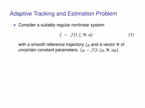
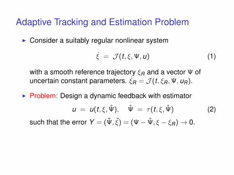
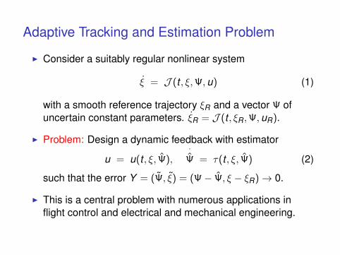
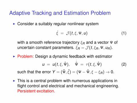
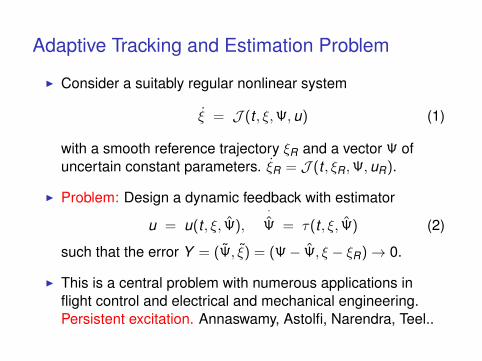
Adaptive Tracking and Estimation Problem
I Consider a suitably regular nonlinear system
ξ = J (t , ξ,Ψ,u) (1)
with a smooth reference trajectory ξR and a vector Ψ ofuncertain constant parameters. ξR = J (t , ξR,Ψ,uR).
I Problem: Design a dynamic feedback with estimator
u = u(t , ξ, Ψ),·
Ψ = τ(t , ξ, Ψ) (2)
such that the error Y = (Ψ, ξ) = (Ψ− Ψ, ξ − ξR)→ 0.
I This is a central problem with numerous applications inflight control and electrical and mechanical engineering.Persistent excitation. Annaswamy, Astolfi, Narendra, Teel..

Adaptive Tracking and Estimation Problem
I Consider a suitably regular nonlinear system
ξ = J (t , ξ,Ψ,u) (1)
with a smooth reference trajectory ξR and a vector Ψ ofuncertain constant parameters.
ξR = J (t , ξR,Ψ,uR).
I Problem: Design a dynamic feedback with estimator
u = u(t , ξ, Ψ),·
Ψ = τ(t , ξ, Ψ) (2)
such that the error Y = (Ψ, ξ) = (Ψ− Ψ, ξ − ξR)→ 0.
I This is a central problem with numerous applications inflight control and electrical and mechanical engineering.Persistent excitation. Annaswamy, Astolfi, Narendra, Teel..
Adaptive Tracking and Estimation Problem
I Consider a suitably regular nonlinear system
ξ = J (t , ξ,Ψ,u) (1)
with a smooth reference trajectory ξR and a vector Ψ ofuncertain constant parameters. ξR = J (t , ξR,Ψ,uR).
I Problem: Design a dynamic feedback with estimator
u = u(t , ξ, Ψ),·
Ψ = τ(t , ξ, Ψ) (2)
such that the error Y = (Ψ, ξ) = (Ψ− Ψ, ξ − ξR)→ 0.
I This is a central problem with numerous applications inflight control and electrical and mechanical engineering.Persistent excitation. Annaswamy, Astolfi, Narendra, Teel..

Adaptive Tracking and Estimation Problem
I Consider a suitably regular nonlinear system
ξ = J (t , ξ,Ψ,u) (1)
with a smooth reference trajectory ξR and a vector Ψ ofuncertain constant parameters. ξR = J (t , ξR,Ψ,uR).
I Problem:
Design a dynamic feedback with estimator
u = u(t , ξ, Ψ),·
Ψ = τ(t , ξ, Ψ) (2)
such that the error Y = (Ψ, ξ) = (Ψ− Ψ, ξ − ξR)→ 0.
I This is a central problem with numerous applications inflight control and electrical and mechanical engineering.Persistent excitation. Annaswamy, Astolfi, Narendra, Teel..
Adaptive Tracking and Estimation Problem
I Consider a suitably regular nonlinear system
ξ = J (t , ξ,Ψ,u) (1)
with a smooth reference trajectory ξR and a vector Ψ ofuncertain constant parameters. ξR = J (t , ξR,Ψ,uR).
I Problem: Design a dynamic feedback with estimator
u = u(t , ξ, Ψ),·
Ψ = τ(t , ξ, Ψ) (2)
such that the error Y = (Ψ, ξ) = (Ψ− Ψ, ξ − ξR)→ 0.
I This is a central problem with numerous applications inflight control and electrical and mechanical engineering.Persistent excitation. Annaswamy, Astolfi, Narendra, Teel..
Adaptive Tracking and Estimation Problem
I Consider a suitably regular nonlinear system
ξ = J (t , ξ,Ψ,u) (1)
with a smooth reference trajectory ξR and a vector Ψ ofuncertain constant parameters. ξR = J (t , ξR,Ψ,uR).
I Problem: Design a dynamic feedback with estimator
u = u(t , ξ, Ψ),·
Ψ = τ(t , ξ, Ψ) (2)
such that the error Y = (Ψ, ξ) = (Ψ− Ψ, ξ − ξR)→ 0.
I This is a central problem with numerous applications inflight control and electrical and mechanical engineering.
Persistent excitation. Annaswamy, Astolfi, Narendra, Teel..
Adaptive Tracking and Estimation Problem
I Consider a suitably regular nonlinear system
ξ = J (t , ξ,Ψ,u) (1)
with a smooth reference trajectory ξR and a vector Ψ ofuncertain constant parameters. ξR = J (t , ξR,Ψ,uR).
I Problem: Design a dynamic feedback with estimator
u = u(t , ξ, Ψ),·
Ψ = τ(t , ξ, Ψ) (2)
such that the error Y = (Ψ, ξ) = (Ψ− Ψ, ξ − ξR)→ 0.
I This is a central problem with numerous applications inflight control and electrical and mechanical engineering.Persistent excitation.
Annaswamy, Astolfi, Narendra, Teel..
Adaptive Tracking and Estimation Problem
I Consider a suitably regular nonlinear system
ξ = J (t , ξ,Ψ,u) (1)
with a smooth reference trajectory ξR and a vector Ψ ofuncertain constant parameters. ξR = J (t , ξR,Ψ,uR).
I Problem: Design a dynamic feedback with estimator
u = u(t , ξ, Ψ),·
Ψ = τ(t , ξ, Ψ) (2)
such that the error Y = (Ψ, ξ) = (Ψ− Ψ, ξ − ξR)→ 0.
I This is a central problem with numerous applications inflight control and electrical and mechanical engineering.Persistent excitation. Annaswamy, Astolfi, Narendra, Teel..

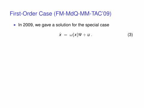
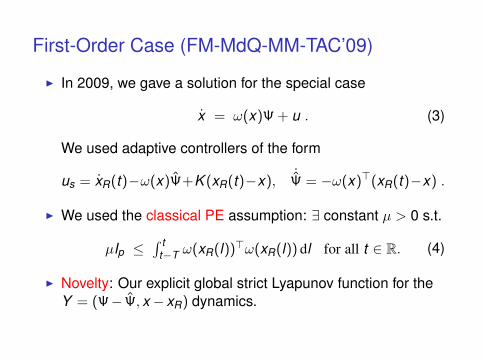
First-Order Case (FM-MdQ-MM-TAC’09)
I In 2009, we gave a solution for the special case
x = ω(x)Ψ + u . (3)
We used adaptive controllers of the form
us = xR(t)−ω(x)Ψ+K (xR(t)−x), ˙Ψ = −ω(x)>(xR(t)−x) .
I We used the classical PE assumption: ∃ constant µ > 0 s.t.
µIp ≤∫ t
t−T ω(xR(l))>ω(xR(l)) dl for all t ∈ R. (4)
I Novelty: Our explicit global strict Lyapunov function for theY = (Ψ− Ψ, x −xR) dynamics. It gave input-to-state stabilitywith respect to additive time-varying uncertainties δ on Ψ.

First-Order Case (FM-MdQ-MM-TAC’09)
I In 2009, we gave a solution for the special case
x = ω(x)Ψ + u . (3)
We used adaptive controllers of the form
us = xR(t)−ω(x)Ψ+K (xR(t)−x), ˙Ψ = −ω(x)>(xR(t)−x) .
I We used the classical PE assumption: ∃ constant µ > 0 s.t.
µIp ≤∫ t
t−T ω(xR(l))>ω(xR(l)) dl for all t ∈ R. (4)
I Novelty:
Our explicit global strict Lyapunov function for theY = (Ψ− Ψ, x −xR) dynamics. It gave input-to-state stabilitywith respect to additive time-varying uncertainties δ on Ψ.
First-Order Case (FM-MdQ-MM-TAC’09)
I In 2009, we gave a solution for the special case
x = ω(x)Ψ + u . (3)
We used adaptive controllers of the form
us = xR(t)−ω(x)Ψ+K (xR(t)−x), ˙Ψ = −ω(x)>(xR(t)−x) .
I We used the classical PE assumption: ∃ constant µ > 0 s.t.
µIp ≤∫ t
t−T ω(xR(l))>ω(xR(l)) dl for all t ∈ R. (4)
I Novelty: Our explicit global strict Lyapunov function for theY = (Ψ− Ψ, x −xR) dynamics.
It gave input-to-state stabilitywith respect to additive time-varying uncertainties δ on Ψ.

First-Order Case (FM-MdQ-MM-TAC’09)
I In 2009, we gave a solution for the special case
x = ω(x)Ψ + u . (3)
We used adaptive controllers of the form
us = xR(t)−ω(x)Ψ+K (xR(t)−x), ˙Ψ = −ω(x)>(xR(t)−x) .
I We used the classical PE assumption: ∃ constant µ > 0 s.t.
µIp ≤∫ t
t−T ω(xR(l))>ω(xR(l)) dl for all t ∈ R. (4)
I Novelty: Our explicit global strict Lyapunov function for theY = (Ψ− Ψ, x −xR) dynamics. It gave input-to-state stabilitywith respect to additive time-varying uncertainties δ on Ψ.

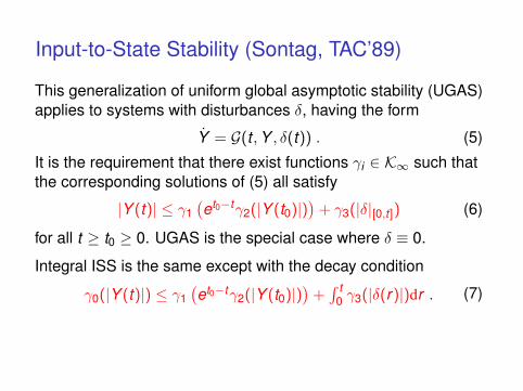
Input-to-State Stability (Sontag, TAC’89)
This generalization of uniform global asymptotic stability (UGAS)applies to systems with disturbances δ, having the form
Y = G(t ,Y , δ(t)) . (5)
It is the requirement that there exist functions γi ∈ K∞ such thatthe corresponding solutions of (5) all satisfy
|Y (t)| ≤ γ1(et0−tγ2(|Y (t0)|)
)+ γ3(|δ|[0,t]) (6)
for all t ≥ t0 ≥ 0. UGAS is the special case where δ ≡ 0.
Integral ISS is the same except with the decay condition
γ0(|Y (t)|) ≤ γ1(et0−tγ2(|Y (t0)|)
)+∫ t
0 γ3(|δ(r)|)dr . (7)
Both are shown by constructing specific kinds of strict Lyapunovfunctions for Y = G(t ,Y ,0).

Input-to-State Stability (Sontag, TAC’89)
This generalization of uniform global asymptotic stability (UGAS)applies to systems with disturbances δ, having the form
Y = G(t ,Y , δ(t)) . (5)
It is the requirement that there exist functions γi ∈ K∞ such thatthe corresponding solutions of (5) all satisfy
|Y (t)| ≤ γ1(et0−tγ2(|Y (t0)|)
)+ γ3(|δ|[0,t]) (6)
for all t ≥ t0 ≥ 0.
UGAS is the special case where δ ≡ 0.
Integral ISS is the same except with the decay condition
γ0(|Y (t)|) ≤ γ1(et0−tγ2(|Y (t0)|)
)+∫ t
0 γ3(|δ(r)|)dr . (7)
Both are shown by constructing specific kinds of strict Lyapunovfunctions for Y = G(t ,Y ,0).

Input-to-State Stability (Sontag, TAC’89)
This generalization of uniform global asymptotic stability (UGAS)applies to systems with disturbances δ, having the form
Y = G(t ,Y , δ(t)) . (5)
It is the requirement that there exist functions γi ∈ K∞ such thatthe corresponding solutions of (5) all satisfy
|Y (t)| ≤ γ1(et0−tγ2(|Y (t0)|)
)+ γ3(|δ|[0,t]) (6)
for all t ≥ t0 ≥ 0. UGAS is the special case where δ ≡ 0.
Integral ISS is the same except with the decay condition
γ0(|Y (t)|) ≤ γ1(et0−tγ2(|Y (t0)|)
)+∫ t
0 γ3(|δ(r)|)dr . (7)
Both are shown by constructing specific kinds of strict Lyapunovfunctions for Y = G(t ,Y ,0).

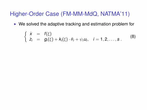
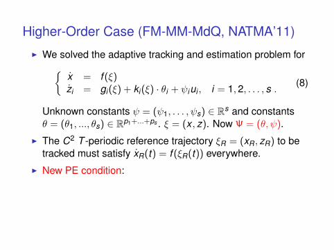
Higher-Order Case (FM-MM-MdQ, NATMA’11)
I We solved the adaptive tracking and estimation problem forx = f (ξ)zi = gi(ξ) + ki(ξ) · θi + ψiui , i = 1,2, . . . , s .
(8)
Unknown constants ψ = (ψ1, . . . , ψs) ∈ Rs and constantsθ = (θ1, ..., θs) ∈ Rp1+...+ps . ξ = (x , z). Now Ψ = (θ, ψ).
I The C2 T -periodic reference trajectory ξR = (xR, zR) to betracked must satisfy xR(t) = f (ξR(t)) everywhere.
I New PE condition: positive definiteness of the matrices
Pidef=∫ T
0 λ>i (t)λi(t) dt ∈ R(pi+1)×(pi+1), (9)
where λi(t) = (ki(ξR(t)), zR,i(t)− gi(ξR(t))) for each i .

Higher-Order Case (FM-MM-MdQ, NATMA’11)
I We solved the adaptive tracking and estimation problem forx = f (ξ)zi = gi(ξ) + ki(ξ) · θi + ψiui , i = 1,2, . . . , s .
(8)
Unknown constants ψ = (ψ1, . . . , ψs) ∈ Rs
and constantsθ = (θ1, ..., θs) ∈ Rp1+...+ps . ξ = (x , z). Now Ψ = (θ, ψ).
I The C2 T -periodic reference trajectory ξR = (xR, zR) to betracked must satisfy xR(t) = f (ξR(t)) everywhere.
I New PE condition: positive definiteness of the matrices
Pidef=∫ T
0 λ>i (t)λi(t) dt ∈ R(pi+1)×(pi+1), (9)
where λi(t) = (ki(ξR(t)), zR,i(t)− gi(ξR(t))) for each i .

Higher-Order Case (FM-MM-MdQ, NATMA’11)
I We solved the adaptive tracking and estimation problem forx = f (ξ)zi = gi(ξ) + ki(ξ) · θi + ψiui , i = 1,2, . . . , s .
(8)
Unknown constants ψ = (ψ1, . . . , ψs) ∈ Rs and constantsθ = (θ1, ..., θs) ∈ Rp1+...+ps .
ξ = (x , z). Now Ψ = (θ, ψ).
I The C2 T -periodic reference trajectory ξR = (xR, zR) to betracked must satisfy xR(t) = f (ξR(t)) everywhere.
I New PE condition: positive definiteness of the matrices
Pidef=∫ T
0 λ>i (t)λi(t) dt ∈ R(pi+1)×(pi+1), (9)
where λi(t) = (ki(ξR(t)), zR,i(t)− gi(ξR(t))) for each i .

Higher-Order Case (FM-MM-MdQ, NATMA’11)
I We solved the adaptive tracking and estimation problem forx = f (ξ)zi = gi(ξ) + ki(ξ) · θi + ψiui , i = 1,2, . . . , s .
(8)
Unknown constants ψ = (ψ1, . . . , ψs) ∈ Rs and constantsθ = (θ1, ..., θs) ∈ Rp1+...+ps . ξ = (x , z).
Now Ψ = (θ, ψ).
I The C2 T -periodic reference trajectory ξR = (xR, zR) to betracked must satisfy xR(t) = f (ξR(t)) everywhere.
I New PE condition: positive definiteness of the matrices
Pidef=∫ T
0 λ>i (t)λi(t) dt ∈ R(pi+1)×(pi+1), (9)
where λi(t) = (ki(ξR(t)), zR,i(t)− gi(ξR(t))) for each i .

Higher-Order Case (FM-MM-MdQ, NATMA’11)
I We solved the adaptive tracking and estimation problem forx = f (ξ)zi = gi(ξ) + ki(ξ) · θi + ψiui , i = 1,2, . . . , s .
(8)
Unknown constants ψ = (ψ1, . . . , ψs) ∈ Rs and constantsθ = (θ1, ..., θs) ∈ Rp1+...+ps . ξ = (x , z). Now Ψ = (θ, ψ).
I The C2 T -periodic reference trajectory ξR = (xR, zR) to betracked must satisfy xR(t) = f (ξR(t)) everywhere.
I New PE condition: positive definiteness of the matrices
Pidef=∫ T
0 λ>i (t)λi(t) dt ∈ R(pi+1)×(pi+1), (9)
where λi(t) = (ki(ξR(t)), zR,i(t)− gi(ξR(t))) for each i .

Higher-Order Case (FM-MM-MdQ, NATMA’11)
I We solved the adaptive tracking and estimation problem forx = f (ξ)zi = gi(ξ) + ki(ξ) · θi + ψiui , i = 1,2, . . . , s .
(8)
Unknown constants ψ = (ψ1, . . . , ψs) ∈ Rs and constantsθ = (θ1, ..., θs) ∈ Rp1+...+ps . ξ = (x , z). Now Ψ = (θ, ψ).
I The C2 T -periodic reference trajectory ξR = (xR, zR) to betracked must satisfy xR(t) = f (ξR(t)) everywhere.
I New PE condition: positive definiteness of the matrices
Pidef=∫ T
0 λ>i (t)λi(t) dt ∈ R(pi+1)×(pi+1), (9)
where λi(t) = (ki(ξR(t)), zR,i(t)− gi(ξR(t))) for each i .
Higher-Order Case (FM-MM-MdQ, NATMA’11)
I We solved the adaptive tracking and estimation problem forx = f (ξ)zi = gi(ξ) + ki(ξ) · θi + ψiui , i = 1,2, . . . , s .
(8)
Unknown constants ψ = (ψ1, . . . , ψs) ∈ Rs and constantsθ = (θ1, ..., θs) ∈ Rp1+...+ps . ξ = (x , z). Now Ψ = (θ, ψ).
I The C2 T -periodic reference trajectory ξR = (xR, zR) to betracked must satisfy xR(t) = f (ξR(t)) everywhere.
I New PE condition:
positive definiteness of the matrices
Pidef=∫ T
0 λ>i (t)λi(t) dt ∈ R(pi+1)×(pi+1), (9)
where λi(t) = (ki(ξR(t)), zR,i(t)− gi(ξR(t))) for each i .

Higher-Order Case (FM-MM-MdQ, NATMA’11)
I We solved the adaptive tracking and estimation problem forx = f (ξ)zi = gi(ξ) + ki(ξ) · θi + ψiui , i = 1,2, . . . , s .
(8)
Unknown constants ψ = (ψ1, . . . , ψs) ∈ Rs and constantsθ = (θ1, ..., θs) ∈ Rp1+...+ps . ξ = (x , z). Now Ψ = (θ, ψ).
I The C2 T -periodic reference trajectory ξR = (xR, zR) to betracked must satisfy xR(t) = f (ξR(t)) everywhere.
I New PE condition: positive definiteness of the matrices
Pidef=∫ T
0 λ>i (t)λi(t) dt ∈ R(pi+1)×(pi+1), (9)
where λi(t) = (ki(ξR(t)), zR,i(t)− gi(ξR(t))) for each i .

Two Other Key Assumptions
I Set F(t , χ) = f (χ+ ξR(t))− f (ξR(t)). There is a feedback vfand a global strict Lyapunov function V for
X = F(t ,X ,Z )
Z = vf (t ,X ,Z )(10)
so that −V and V have positive definite quadratic lowerbounds near 0 and V , and vf are T -periodic.
Backstepping.. See Sontag text, Chap. 5.
I There are known positive constants θM , ψ and ψ such that
ψ < ψi < ψ and |θi | < θM (11)
for each i ∈ 1,2, . . . , s. Known directions for the ψi ’s.

Two Other Key Assumptions
I Set F(t , χ) = f (χ+ ξR(t))− f (ξR(t)).
There is a feedback vfand a global strict Lyapunov function V for
X = F(t ,X ,Z )
Z = vf (t ,X ,Z )(10)
so that −V and V have positive definite quadratic lowerbounds near 0 and V , and vf are T -periodic.
Backstepping.. See Sontag text, Chap. 5.
I There are known positive constants θM , ψ and ψ such that
ψ < ψi < ψ and |θi | < θM (11)
for each i ∈ 1,2, . . . , s. Known directions for the ψi ’s.

Two Other Key Assumptions
I Set F(t , χ) = f (χ+ ξR(t))− f (ξR(t)). There is a feedback vfand a global strict Lyapunov function V for
X = F(t ,X ,Z )
Z = vf (t ,X ,Z )(10)
so that −V and V have positive definite quadratic lowerbounds near 0
and V , and vf are T -periodic.
Backstepping.. See Sontag text, Chap. 5.
I There are known positive constants θM , ψ and ψ such that
ψ < ψi < ψ and |θi | < θM (11)
for each i ∈ 1,2, . . . , s. Known directions for the ψi ’s.

Two Other Key Assumptions
I Set F(t , χ) = f (χ+ ξR(t))− f (ξR(t)). There is a feedback vfand a global strict Lyapunov function V for
X = F(t ,X ,Z )
Z = vf (t ,X ,Z )(10)
so that −V and V have positive definite quadratic lowerbounds near 0 and V , and vf are T -periodic.
Backstepping.. See Sontag text, Chap. 5.
I There are known positive constants θM , ψ and ψ such that
ψ < ψi < ψ and |θi | < θM (11)
for each i ∈ 1,2, . . . , s. Known directions for the ψi ’s.

Two Other Key Assumptions
I Set F(t , χ) = f (χ+ ξR(t))− f (ξR(t)). There is a feedback vfand a global strict Lyapunov function V for
X = F(t ,X ,Z )
Z = vf (t ,X ,Z )(10)
so that −V and V have positive definite quadratic lowerbounds near 0 and V , and vf are T -periodic.
Backstepping..
See Sontag text, Chap. 5.
I There are known positive constants θM , ψ and ψ such that
ψ < ψi < ψ and |θi | < θM (11)
for each i ∈ 1,2, . . . , s. Known directions for the ψi ’s.

Two Other Key Assumptions
I Set F(t , χ) = f (χ+ ξR(t))− f (ξR(t)). There is a feedback vfand a global strict Lyapunov function V for
X = F(t ,X ,Z )
Z = vf (t ,X ,Z )(10)
so that −V and V have positive definite quadratic lowerbounds near 0 and V , and vf are T -periodic.
Backstepping.. See Sontag text, Chap. 5.
I There are known positive constants θM , ψ and ψ such that
ψ < ψi < ψ and |θi | < θM (11)
for each i ∈ 1,2, . . . , s. Known directions for the ψi ’s.

Two Other Key Assumptions
I Set F(t , χ) = f (χ+ ξR(t))− f (ξR(t)). There is a feedback vfand a global strict Lyapunov function V for
X = F(t ,X ,Z )
Z = vf (t ,X ,Z )(10)
so that −V and V have positive definite quadratic lowerbounds near 0 and V , and vf are T -periodic.
Backstepping.. See Sontag text, Chap. 5.
I There are known positive constants θM , ψ and ψ such that
ψ < ψi < ψ and |θi | < θM (11)
for each i ∈ 1,2, . . . , s.
Known directions for the ψi ’s.

Two Other Key Assumptions
I Set F(t , χ) = f (χ+ ξR(t))− f (ξR(t)). There is a feedback vfand a global strict Lyapunov function V for
X = F(t ,X ,Z )
Z = vf (t ,X ,Z )(10)
so that −V and V have positive definite quadratic lowerbounds near 0 and V , and vf are T -periodic.
Backstepping.. See Sontag text, Chap. 5.
I There are known positive constants θM , ψ and ψ such that
ψ < ψi < ψ and |θi | < θM (11)
for each i ∈ 1,2, . . . , s. Known directions for the ψi ’s.

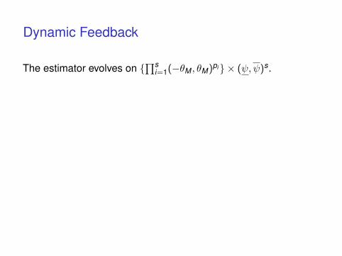
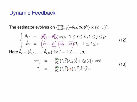
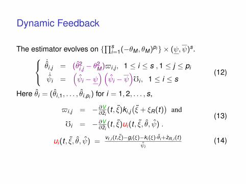
Dynamic Feedback
The estimator evolves on ∏s
i=1(−θM , θM)pi × (ψ,ψ)s.˙θi,j = (θ2
i,j − θ2M)$i,j , 1 ≤ i ≤ s ,1 ≤ j ≤ pi
˙ψi =
(ψi − ψ
)(ψi − ψ
)fi , 1 ≤ i ≤ s
(12)
Here θi = (θi,1, . . . , θi,pi ) for i = 1,2, . . . , s,
$i,j = −∂V∂zi
(t , ξ)ki,j(ξ + ξR(t)
)and
fi = −∂V∂zi
(t , ξ)ui(t , ξ, θ, ψ) .(13)
ui(t , ξ, θ, ψ) =vf ,i (t ,ξ)−gi (ξ)−ki (ξ)·θi+zR,i (t)
ψi(14)
The estimator and feedback can only depend on things we know.
Dynamic Feedback
The estimator evolves on ∏s
i=1(−θM , θM)pi × (ψ,ψ)s.
˙θi,j = (θ2
i,j − θ2M)$i,j , 1 ≤ i ≤ s ,1 ≤ j ≤ pi
˙ψi =
(ψi − ψ
)(ψi − ψ
)fi , 1 ≤ i ≤ s
(12)
Here θi = (θi,1, . . . , θi,pi ) for i = 1,2, . . . , s,
$i,j = −∂V∂zi
(t , ξ)ki,j(ξ + ξR(t)
)and
fi = −∂V∂zi
(t , ξ)ui(t , ξ, θ, ψ) .(13)
ui(t , ξ, θ, ψ) =vf ,i (t ,ξ)−gi (ξ)−ki (ξ)·θi+zR,i (t)
ψi(14)
The estimator and feedback can only depend on things we know.

Dynamic Feedback
The estimator evolves on ∏s
i=1(−θM , θM)pi × (ψ,ψ)s.˙θi,j = (θ2
i,j − θ2M)$i,j , 1 ≤ i ≤ s ,1 ≤ j ≤ pi
˙ψi =
(ψi − ψ
)(ψi − ψ
)fi , 1 ≤ i ≤ s
(12)
Here θi = (θi,1, . . . , θi,pi ) for i = 1,2, . . . , s,
$i,j = −∂V∂zi
(t , ξ)ki,j(ξ + ξR(t)
)and
fi = −∂V∂zi
(t , ξ)ui(t , ξ, θ, ψ) .(13)
ui(t , ξ, θ, ψ) =vf ,i (t ,ξ)−gi (ξ)−ki (ξ)·θi+zR,i (t)
ψi(14)
The estimator and feedback can only depend on things we know.

Dynamic Feedback
The estimator evolves on ∏s
i=1(−θM , θM)pi × (ψ,ψ)s.˙θi,j = (θ2
i,j − θ2M)$i,j , 1 ≤ i ≤ s ,1 ≤ j ≤ pi
˙ψi =
(ψi − ψ
)(ψi − ψ
)fi , 1 ≤ i ≤ s
(12)
Here θi = (θi,1, . . . , θi,pi ) for i = 1,2, . . . , s
,
$i,j = −∂V∂zi
(t , ξ)ki,j(ξ + ξR(t)
)and
fi = −∂V∂zi
(t , ξ)ui(t , ξ, θ, ψ) .(13)
ui(t , ξ, θ, ψ) =vf ,i (t ,ξ)−gi (ξ)−ki (ξ)·θi+zR,i (t)
ψi(14)
The estimator and feedback can only depend on things we know.

Dynamic Feedback
The estimator evolves on ∏s
i=1(−θM , θM)pi × (ψ,ψ)s.˙θi,j = (θ2
i,j − θ2M)$i,j , 1 ≤ i ≤ s ,1 ≤ j ≤ pi
˙ψi =
(ψi − ψ
)(ψi − ψ
)fi , 1 ≤ i ≤ s
(12)
Here θi = (θi,1, . . . , θi,pi ) for i = 1,2, . . . , s,
$i,j = −∂V∂zi
(t , ξ)ki,j(ξ + ξR(t)
)
and
fi = −∂V∂zi
(t , ξ)ui(t , ξ, θ, ψ) .(13)
ui(t , ξ, θ, ψ) =vf ,i (t ,ξ)−gi (ξ)−ki (ξ)·θi+zR,i (t)
ψi(14)
The estimator and feedback can only depend on things we know.
Dynamic Feedback
The estimator evolves on ∏s
i=1(−θM , θM)pi × (ψ,ψ)s.˙θi,j = (θ2
i,j − θ2M)$i,j , 1 ≤ i ≤ s ,1 ≤ j ≤ pi
˙ψi =
(ψi − ψ
)(ψi − ψ
)fi , 1 ≤ i ≤ s
(12)
Here θi = (θi,1, . . . , θi,pi ) for i = 1,2, . . . , s,
$i,j = −∂V∂zi
(t , ξ)ki,j(ξ + ξR(t)
)and
fi = −∂V∂zi
(t , ξ)ui(t , ξ, θ, ψ) .(13)
ui(t , ξ, θ, ψ) =vf ,i (t ,ξ)−gi (ξ)−ki (ξ)·θi+zR,i (t)
ψi(14)
The estimator and feedback can only depend on things we know.

Stabilization Analysis
I We build a global strict Lyapunov function for theY = (ξ, θ, ψ) = (ξ − ξR, θ − θ, ψ − ψ) dynamics to prove theUGAS condition |Y (t)| ≤ γ1(et0−tγ2(|Y (t0)|)).
I We start with the nonstrict Lyapunov function
V1(t , ξ, θ, ψ) = V (t , ξ) +s∑
i=1
pi∑j=1
∫ θi,j
0
mθ2
M − (m − θi,j)2dm
+s∑
i=1
∫ ψi
0
m(ψi −m − ψ)(ψ − ψi + m)
dm .
I It gives V1 ≤ −W (ξ) for some positive definite function W .
I This is insufficient for robustness analysis because V1 couldbe zero outside 0. Therefore, we transform V1.

Stabilization Analysis
I We build a global strict Lyapunov function for theY = (ξ, θ, ψ) = (ξ − ξR, θ − θ, ψ − ψ) dynamics to prove theUGAS condition |Y (t)| ≤ γ1(et0−tγ2(|Y (t0)|)).
I We start with the nonstrict Lyapunov function
V1(t , ξ, θ, ψ) = V (t , ξ) +s∑
i=1
pi∑j=1
∫ θi,j
0
mθ2
M − (m − θi,j)2dm
+s∑
i=1
∫ ψi
0
m(ψi −m − ψ)(ψ − ψi + m)
dm .
I It gives V1 ≤ −W (ξ) for some positive definite function W .
I This is insufficient for robustness analysis because V1 couldbe zero outside 0.
Therefore, we transform V1.

Stabilization Analysis
I We build a global strict Lyapunov function for theY = (ξ, θ, ψ) = (ξ − ξR, θ − θ, ψ − ψ) dynamics to prove theUGAS condition |Y (t)| ≤ γ1(et0−tγ2(|Y (t0)|)).
I We start with the nonstrict Lyapunov function
V1(t , ξ, θ, ψ) = V (t , ξ) +s∑
i=1
pi∑j=1
∫ θi,j
0
mθ2
M − (m − θi,j)2dm
+s∑
i=1
∫ ψi
0
m(ψi −m − ψ)(ψ − ψi + m)
dm .
I It gives V1 ≤ −W (ξ) for some positive definite function W .
I This is insufficient for robustness analysis because V1 couldbe zero outside 0. Therefore, we transform V1.

Transformation (FM-MM-MdQ, NATMA’11)
Theorem: We can construct K ∈ K∞ ∩ C1 such that
V ](t , ξ, θ, ψ).
= K(V1(t , ξ, θ, ψ)
)+
s∑i=1
Υi(t , ξ, θ, ψ) , (15)
where Υi(t , ξ, θ, ψ) = −ziλi(t)αi(θi , ψi)
+ 1Tψα>i (θi , ψi)Ωi(t)αi(θi , ψi) ,
(16)
λi(t) = (ki(ξR(t)), zR,i(t)− gi(ξR(t))) , (17)
αi(θi , ψi) =
[θiψi − θi ψi
ψi
], and
Ωi(t) =∫ t
t−T
∫ tm λ>i (s)λi(s)ds dm ,
(18)
is a global strict Lyapunov function for the Y = (ξ, θ, ψ)dynamics. Hence, the dynamics are UGAS to 0.

Transformation (FM-MM-MdQ, NATMA’11)Theorem: We can construct K ∈ K∞ ∩ C1 such that
V ](t , ξ, θ, ψ).
= K(V1(t , ξ, θ, ψ)
)+
s∑i=1
Υi(t , ξ, θ, ψ) , (15)
where Υi(t , ξ, θ, ψ) = −ziλi(t)αi(θi , ψi)
+ 1Tψα>i (θi , ψi)Ωi(t)αi(θi , ψi) ,
(16)
λi(t) = (ki(ξR(t)), zR,i(t)− gi(ξR(t))) , (17)
αi(θi , ψi) =
[θiψi − θi ψi
ψi
], and
Ωi(t) =∫ t
t−T
∫ tm λ>i (s)λi(s)ds dm ,
(18)
is a global strict Lyapunov function for the Y = (ξ, θ, ψ)dynamics.
Hence, the dynamics are UGAS to 0.

Transformation (FM-MM-MdQ, NATMA’11)Theorem: We can construct K ∈ K∞ ∩ C1 such that
V ](t , ξ, θ, ψ).
= K(V1(t , ξ, θ, ψ)
)+
s∑i=1
Υi(t , ξ, θ, ψ) , (15)
where Υi(t , ξ, θ, ψ) = −ziλi(t)αi(θi , ψi)
+ 1Tψα>i (θi , ψi)Ωi(t)αi(θi , ψi) ,
(16)
λi(t) = (ki(ξR(t)), zR,i(t)− gi(ξR(t))) , (17)
αi(θi , ψi) =
[θiψi − θi ψi
ψi
], and
Ωi(t) =∫ t
t−T
∫ tm λ>i (s)λi(s)ds dm ,
(18)
is a global strict Lyapunov function for the Y = (ξ, θ, ψ)dynamics. Hence, the dynamics are UGAS to 0.

Conclusions
I Adaptive tracking and estimation is a central problem withapplications in many branches of engineering.
I Standard adaptive control treatments based on nonstrictLyapunov functions only give tracking and are not robust.
I Our strict Lyapunov functions gave robustness to additiveuncertainties on the parameters using the ISS paradigm.
I We covered systems with unknown control gains includingbrushless DC motors turning mechanical loads.
I It would be useful to extend to cover models that are notaffine in θ, feedback delays, and output feedbacks.


![An Online Parameter Estimation Tool · # Nonlinear state function $ Nonlinear observer function Tailplane trim angle ... identification and hence parameter estimation effort [9,10]](https://img.dokumen.tips/doc/110x75/5e86752d23474e477705949f/an-online-parameter-estimation-tool-nonlinear-state-function-nonlinear-observer.jpg)