Estimation of Nonlinear Models with MismeasuredRegressors Using Marginal Information

Yingyao HuJohns Hopkins University

Geert RidderUniversity of Southern California

June 2009

Abstract

We consider the estimation of nonlinear models with mismeasured explanatory vari-ables, when information on the marginal distribution of the true values of these vari-ables is available. We derive a semi-parametric MLE that is shown to be

pn consistent

and asymptotically normally distributed. In a simulation experiment we �nd that the�nite sample distribution of the estimator is close to the asymptotic approximation.The semi-parametric MLE is applied to a duration model for AFDC welfare spells withmisreported welfare bene�ts. The marginal distribution of the correctly measured wel-fare bene�ts is obtained from an administrative source.JEL classi�cation: C14, C41, I38.Keywords: measurement error model, marginal information, deconvolution, Fourier

transform, duration model, welfare spells.

1 Introduction

Many models that are routinely used in empirical research in microeconomics are nonlinear in

the explanatory variables. Examples are nonlinear (in variables) regression models, models

for limited-dependent variables (logit, probit, tobit etc.), and duration models. Often the

parameters of such nonlinear models are estimated using economic data in which one or more

independent variables are measured with error (Bound, Brown, and Mathiowetz, 2001). The

identi�cation and estimation of models that are nonlinear in mismeasured variables is a

notoriously di¢ cult problem (see Carroll, Ruppert, and Stefanski (1995) for a survey).

There are three approaches to this problem: (i) the parametric approach, (ii) the instru-

mental variable method, and (iii) methods that use an additional sample, such as a validation

sample. Throughout we assume that we have a parametric model for the relation between

the dependent and independent variables, but that we want to make minimal assumptions

on the measurement errors and the distribution of the explanatory variables.

The parametric approach makes strong and untestable distributional assumptions. In

particular, it is assumed that the distribution of the measurement error is in some parametric

class (Bickel and Ritov, 1987; Hsiao, 1989, 1991; Cheng and Van Ness, 1994; Murphy and

Van Der Vaart, 1996; Wang, 1998; Kong and Gu, 1999; Hsiao and Wang, 2000; Augustin,

2004). With this assumption the estimation problem is complicated, but fully parametric.

The second approach is the instrumental variable method. In an errors-in-variables model,

a valid instrument is a variable that (a) can be excluded from the model, (b) is correlated

with the latent true value, and (c) is independent of the measurement error (Amemiya and

Fuller, 1988; Carroll and Stefanski, 1990; Hausman, Ichimura, Newey, and Powell, 1991;

Hausman, Newey, and Powell, 1995; Li and Vuong, 1998; Newey, 2001). Schennach (2004,

2007) and Hu and Schennach (2006) extend the IV estimator to general nonlinear models.

The third approach is to use an additional sample, such as a validation sample (Bound,

Brown, Duncan, and Rodgers, 1989; Hsiao, 1989; Hausman, Ichimura, Newey, and Powell,

1991; Pepe and Fleming, 1991; Carroll and Wand, 1991; Lee and Sepanski, 1995; Chen,

Hong and Tamer 2005). A validation sample is a subsample of the original sample for which

accurate measurements are available. The approach taken in this paper is along these lines.

In this paper we show that much of the bene�ts of a validation sample can be obtained if

we have a random sample from the marginal distribution of the mismeasured variables, i.e.

we need not observe the mismeasured and true value and the other independent variables

for the same units. Information on the marginal distribution of the true value is available

in administrative registers, as employer�s records, tax returns, quality control samples, med-

ical records, unemployment insurance and social security records, and �nancial institution

1

records. In fact, most validation samples are constructed by matching survey data to ad-

ministrative data. Creating such matched samples is very costly and sometimes impossible.

Moreover, the owners of the administrative data may be reluctant to release the data because

the matching raises privacy issues. Our approach only requires a random sample from the

administrative register. Indeed the random sample and the survey need not have any unit in

common. Of course, if available a validation sample is preferable over marginal information.

With a validation sample the assumptions on the measurement error can be substantially

weaker than with marginal information. Because we do not observe the mismeasured and

accurate variables for the same units, marginal information cannot identify the correlation

between the measurement error and the true value. For that reason we maintain the as-

sumption of classical measurement error, i.e. the measurement error is independent of the

true value and also independent of the other covariates in the model. The latter assumption

can be relaxed if these covariates are common to the survey sample and the administrative

data. Validation studies have found that the assumption of classical measurement errors

may not hold in practice (see e.g. Bound, Brown, Duncan, and Rodgers (1989)). The main

advantage of a validation sample over marginal information is that it allows us to avoid

this assumption. However, as with a validation sample, marginal information allows us to

avoid assumptions on the distribution of the measurement error and the latent true value.

Given the scarcity of validation samples relative to administrative data sets, the correction

developed in this paper can be more widely applied, but researchers must be aware that the

estimates are biased if the assumptions on the measurement error do not hold1.

In recent years many studies have used administrative data, because they are considered

to be more accurate. For example, employer�s records have been used to study annual earn-

ings and hourly wages (Angrist and Krueger, 1999; Bound, Brown, Duncan, and Rodgers,

1994), union coverage (Barron, Berger, and Black, 1997), and unemployment spells (Math-

iowetz and Duncan, 1988). Tax returns have been used in studies of wage and income (Code,

1992), unemployment bene�ts (Dibbs, Hale, Loverock, and Michaud, 1995), and asset own-

ership and interest income (Grondin and Michaud, 1994). Cohen and Carlson (1994) study

health care expenditures using medical records, and Johnson and Sanchez (1993) use these

records to study health outcomes. Transcript data have been used to study years of schooling

(Kane, Rouse and Staiger, 1999). Card, Hildreth, and Shore-Sheppard (2001) examine Med-

icaid coverage using Medicaid data. Bound, Brown, and Mathiowetz (2001) give a survey

of studies that use administrative data. A problem with administrative records is that they

usually contain only a small number of variables. We show that the marginal distribution

1It is possible to apply the estimator developed in this paper with a level of dependence between the truevalue and the measurement error. In that case prior knowledge must be used to set the degree of dependence.

2

of the latent true values from administrative records is su¢ cient to correct for measurement

error in a survey sample. There have been earlier attempts to combine combine survey and

administrative data to deal with the measurement error in survey data. In the 70�s statis-

tical matching of surveys and administrative �les without common units was used to create

synthetic data sets that contained the accurate data. Ridder and Mo¢ tt (2003) survey this

literature. This paper can be considered as a better approach to the use of accurate data

from a secondary source to deal with measurement error.

Our application indicates what type of data can be used. We consider a duration model

for the relation between welfare bene�ts and the length of welfare spells. The survey data

are from the Survey of Income and Program Participation (SIPP). The welfare bene�ts in

the SIPP are self-reported and are likely to contain reporting errors. The federal government

requires the states to report random samples from their welfare records to check whether the

welfare bene�ts are calculated correctly. The random samples are publicly available as the

AFDC Quality Control Survey (AFDC QC). For that reason they do not contain identi�ers

that could be used to match the AFDC QC to the SIPP, a task that would yield a small

sample anyway because of the lack of overlap of the two samples. Besides the welfare bene�ts

the AFDC QC contains only a few other variables.

This paper shows that the combination of a sample survey in which some of the inde-

pendent variables are measured with error and a secondary data set that contains a sample

from the marginal distribution of the latent true values of the mismeasured variables iden-

ti�es the conditional distribution of the latent true value given the reported value and the

other independent variables. This distribution is used to integrate out the latent true val-

ues from the model. The resulting mixture model (with estimated mixing distribution)

can then be estimated by Maximum Likelihood (ML) (or Generalized Method of Moments

(GMM)). The semi-parametric MLE (GMM estimator) ispn consistent.2 We derive its as-

ymptotic variance that accounts for the fact that the mixing distribution is estimated. The

semi-parametric MLE avoids any assumption on the distribution of the measurement error

and/or the distribution of the latent true value.

The paper is organized as follows. Section 2 establishes non-parametric identi�cation.

Section 3 gives the estimator and its properties. Section 4 presents Monte Carlo evidence on

the �nite sample performance of the estimator. An empirical application is given in section

5. Section 6 contains extensions and conclusions. The proofs are in the appendix.

2Our semi-parametric MLE involves two deconvolutions. The use of deconvolution estimators in the �rststage is potentially problematic (Taupin, 2001). We apply the results in Hu and Ridder (2005) who showthat

pn consistency can be obtained if the distribution of the measurement error is range-restricted.

3

2 Identi�cation using marginal information

A parametric model for the relation between a dependent variable y, a latent true vari-

able x� and other covariates w can be expressed as a conditional density of y given x�; w,

f �(yjx�; w; �). The relation between the observed x and the latent x� is

x = x� + " (1)

with the classical measurement error assumption " ? x�; w; y where ? indicates stochastic

independence. In the linear regression model the independence of the measurement error

and y given x�; w, which is implied by this assumption, is equivalent to the independence of

the measurement error and the regression error. The variable x� (and hence x) is continuous.

The independent variables in w can be either discrete or continuous. To keep the notation

simple, the theory will be developed for the case that w is scalar.

The data are a random sample yi; xi; wi; i = 1; : : : ; n from the joint distribution of y; x; w,

the survey data, and a random sample x�i ; i = 1; : : : ; n1 from the marginal distribution of x�,

the secondary sample that in most cases is a random sample from an administrative �le. In

asymptotic arguments we assume that both n; n1 become large and that their ratio converges

to a positive and �nite number.

E¢ cient inference for the parameters � is based on the likelihood function. The individual

contribution to the likelihood is the conditional density of y given x;w, f(yjx;w; �). Therelation between this density and that of the parametric model is

f(yjx;w; �) =ZX �f �(yjx�; w; �)g(x�jx;w)dx� (2)

The conditional density g(x�jx;w) does not depend on �, because x�; w is assumed to be

ancillary for �, and the measurement error is independent of y given x�; w.

The key problem with the use of the conditional density (2) in likelihood inference is that

it requires knowledge of the density g(x�jx;w). This density can be expressed as

g(x�jx;w) = g(xjx�; w)g2(x�; w)g(x;w)

(3)

For likelihood inference we must identify the densities g(xjx�; w) and g2(x�; w), while thedensity in the denominator does not a¤ect the inference. We could choose a parametric

density for g(x�jx;w) and estimate its parameters jointly with �. There are at least twoproblems with that approach. First, it is not clear whether the parameters in the density are

identi�ed, and if so, whether the identi�cation is by the arbitrary distributional assumptions

4

and/or the functional form of the parametric model. If there is (parametric) identi�cation,

misspeci�cation of g(x�jx;w) will bias the MLE of �. Second, empirical researchers are

reluctant to make distributional assumptions on the independent variables in conditional

models. For that reason we consider non-parametric identi�cation and estimation of the

density of x� given x;w.

We have to show that the densities in the numerator are non-parametrically identi�ed.

First, the assumption that the measurement error " is independent of x�; w implies that

g(xjx�; w) = g1(x� x�) (4)

with g1 the density of ". Because the observed x is the convolution, i.e. sum, of the

latent true value and the measurement error, it is convenient to work with the characteristic

function of the random variables, instead of their density or distribution functions. Of course,

there is a one-to-one correspondence between characteristic functions and distributions. Let

�x(t) = E(exp(itx)) be the characteristic function of the random variable x. From (1) and

the assumption that x� and " are independent we have �x(t) = �x�(t)�"(t). Hence, if the

marginal distribution of x� is known, we can solve for the characteristic function of the

measurement error distribution

�"(t) =�x(t)

�x�(t)(5)

Because of the one-to-one correspondence between characteristic functions and distributions,

this identi�es g(xjx�; w). By the law of total probability the density g2(x�; w) is related tothe density g(x;w) as

g(x;w) =

ZX �g(xjx�; w)g2(x�; w)dx� =

ZX �g1(x� x�)g2(x

�; w)dx� (6)

This implies that the joint characteristic function �xw(r; s) = E(exp(irx + isw)) of the

distribution of x;w, is equal to (with a change of variables to " = x� x�)

�xw(r; s) =

ZW

ZX �

ZXeir(x�x

�)g1(x� x�)dxeirx�+iswg2(x

�; w)dx�dw = �"(r)�x�w(r; s)

so that

�x�;w(r; s) =�x;w(r; s)

�"(r)=�x;w(r; s)�x�(r)

�x(r)(7)

If the data consist of a primary sample from the joint distribution of y; x; w and a secondary

sample from the marginal distribution of x�, then the right-hand side of (7) contains only

characteristic functions of distributions that can be observed in either sample.

5

The conditional density in (2) is a mixture with a mixing distribution that can be iden-

ti�ed from the joint distribution of x;w and the marginal distribution of x�. We still must

establish that � can be identi�ed from this mixture. The parametric model for the relation

between y and x�; w, speci�es the conditional density of y given x�; w, f �(yjx�; w; �). Theparameters in this model are identi�ed, if for all � 6= �0 with �0 the population value of the

parameter vector, there is a set A(�) with positive measure, such that for (y; x�; w) 2 A(�),f �(yjx�; w; �) 6= f �(yjx�; w; �0). If the parameters are identi�ed, then the expected (with re-spect to the population distribution of y; x�; w) log likelihood has a unique and well-separated

maximum in �0 (Van Der Vaart (1998), Lemma 5.35).

Under weak assumptions on the distribution of the measurement error, identi�cation of

� in f �(yjx�; w; �) implies identi�cation of � in f(yjx;w; �).

Theorem 1 If (i) �0 is identi�ed if we observe y; x�; w, (ii) the characteristic function of "has a countable number of zeros, and (iii) the density of x�; w and f �(yjx�; w; �) have twointegrable derivatives with respect to x�, then �0 is identi�ed if we observe y; x; w.

Proof See appendix.

The fact that the density of x� given x;w is non-parametrically identi�ed makes it possible

to study e.g. non-parametric regression of y on x�; w using data from the joint distribution

of y; w and the marginal distribution of x�. This is beyond the scope of the present paper

that considers only parametric models. However, it must be stressed that the conditional

density of y given x�; w is non-parametrically identi�ed, so that we do not rely on functional

form or distributional assumptions in the identi�cation of �.

3 Estimation with marginal information

3.1 Non-parametric Fourier inversion estimators

Our estimator is a two-step semi-parametric estimator. The �rst step in the estimation is to

obtain a non-parametric estimator of g1(x�x�)g2(x�; w). The density g1 of the measurementerror " has characteristic function, abbreviated as cf, �"(t) =

�x(t)�x� (t)

. The operation by which

the cf of one of the random variables in a convolution is obtained from the cf of the sum and

the cf of the other component is called deconvolution. By Fourier inversion we have, if �" is

absolutely integrable (see below),

g1(x� x�) =1

2�

Z 1

�1e�it(x�x

�) �x(t)

�x�(t)dt (8)

6

The joint characteristic function of x�; w is �x�w(r; s) =�xw(r;s)�x� (r)

�x(r). Again Fourier

inversion gives, if �x�w is absolutely integrable, the joint density of x�; w as

g2(x�; w) =

1

(2�)2

Z 1

�1

Z 1

�1e�irx

��isw�xw(r; s)�x�(r)

�x(r)drds (9)

The Fourier inversion formulas become non-parametric estimators, if we replace the cf

by empirical characteristic functions (ecf). If we have a random sample xi; i = 1; : : : ; n from

the distribution of x, then the ecf is de�ned as

�x(t) =1

n

nXi=1

eitxi

However, the estimators that we obtain if we substitute the ecf of x and x� in (8) and the

ecf of x;w, x� and x in (9) are not well-de�ned. In particular, sampling variations cause the

integrals not to converge. Moreover, to prove consistency of the estimators we need results

on the uniform convergence of the empirical cf (as a function of t). Uniform convergence for

�1 < t <1 cannot be established. For these reasons we introduce integration limits in the

de�nition of the non-parametric density estimators by multiplying the integrand by a weight

function K�n(t) that is 0 for jtj > Tn. For reasons that will become clear, we choose K�

n(t) =

K�( tTn) withK� the Fourier transform of the functionK, i.e. K�(t) =

R1�1 e

�itzK(z)dz. The

functionK is a kernel that satis�es: (i)K(z) = K(�z) andK2 is integrable; (ii)K�(t) = 0 for

jtj > 1, (iii)R1�1K(z)dz = 1,

R1�1 z

jK(z)dz = 0 for j = 1; 2; :::; q�1; andR1�1 jzj

qK(z)dz <

1, i.e. K is a kernel of order q. In the nonparametric density estimator of x�; w we multiply

by a bivariate weight function K�n(r; s) = K�( r

Rn; sSn) with K�(r; s) the bivariate Fourier

transform of the kernel K(v; z) that satis�es (i)-(ii), and (iii)R1�1R1�1K(v; z)dzdv = 1,R1

�1R1�1 v

kzlK(v; z)dzdv = 0 if k+1 < q andR1�1R1�1 jvj

kjzjlK(v; z)dzdv <1 if k+ l = q.

With these weight functions the nonparametric density estimators are

g1(x� x�) =1

2�

Z 1

�1e�it(x�x

�) �x(t)

�x�(t)K�n(t)dt: (10)

g2(x�; w) =

1

4�2

Z 1

�1

Z 1

�1e�irx

��isw �xw(r; s)�x�(r)

�x(r)K�n(r; s)dsdr; (11)

The implicit integration limits Tn; Rn; and Sn diverge at an appropriate rate to be de�ned

below. Although we integrate a complex-valued function the integrals are real3. However,

3Because eitxj = cos(txj)+ isin(txj) the ecf has a real part that is an even function of t and an imaginarypart that is an odd function of t. Let Ek(t) for k = 1; 2; 3; 4 be real even functions in t, i.e. Ek(t) = Ek(�t),

7

because we truncate the range of integration, the estimated densities need not be positive.

Figure 4 illustrates this for our application.

Demonstration of consistency of the non-parametric estimators in (10) and (11) requires

some restrictions on the distributions of x� and ". A relatively weak restriction is that

the cf of " and that of x�; w must be absolutely integrable, i.e.R1�1 j�"(t)jdt < 1 andR1

�1R1�1 j�x�w(r; s)jdrds < 1. A su¢ cient condition is that e.g.

R1�1 jg1(")

00jd" < 1 with

g001 the second derivative of the pdf of " , which is a weak smoothness condition (and an

analogous condition on the joint density of x;w).

A second restriction derives from the fact that deconvolution involves division by an (em-

pirical) characteristic function. For this reason a common assumption in the deconvolution

literature is that the characteristic function in the denominator is never equal to 0. For

instance, the characteristic function of the normal distribution with mean 0 has this prop-

erty. This assumption is not necessary to ensure the consistency of the semiparametric MLE.

However, we have been unable to provepn consistency of the semi-parametric MLE without

it. The assumption is not innocuous, because it excludes e.g. the symmetrically truncated

normal distribution (with mean 0). To ensurepn consistency we restrict the distributions

whose cf appears in the denominator to the class of range-restricted distributions. Because

these distributions are asymmetrically truncated, their cf-s do not have (real) zeroes. The

nonzero cf assumption is a peculiarity of the deconvolution approach to the solution of lin-

ear integral equations. Its resolution may require a di¤erent solution method for the linear

integral equations that determine the densities of " and of x�; w. This is beyond the scope

of the present paper.

Finally, to obtain a rate of convergence of the �rst-stage nonparametric density estimators

that is fast enough to ensurepn consistency of the semi-parametric MLE the characteristic

functions of x� and " must be ordinarily smooth (Fan, 1991), i.e. for large t the characteristic

functions must be such that for some C0; C1; k > 0

C0t�(k+1) � j�v(t)j � C1t

�(k+1);

where t may be a vector. Let Ok(t) for k = 1; 2; 3; 4 be real odd functions in t, i.e. Ok(�t) = �Ok(t). Forany E1(t); E2(t); O1(t); O2(t), we have that

[E1(t) + iO1(t)] [E2(t) + iO2(t)] = E3(t) + iO3(t);

andE1(t) + iO1(t)

E2(t) + iO2(t)= E4(t) + iO4(t):

Let the even functions and the odd functions be the real and the imaginary part of the ecf. Then themultiplication/division of ecf results in functions with an imaginary part that is an odd function of t. Thisimplies that the imaginary part of the integrand is an odd function of t so that its integral is 0.

8

The integer k is the index of smoothness. In the deconvolution literature assumptions on

the tail behavior of characteristic functions are common. Hu and Ridder (2005) relate these

assumptions to the underlying distributions. They show that a su¢ cient condition is that

distributions of the latent true value x� and the measurement error " are range-restricted

(Hu and Ridder, 2005).The distribution of a random variable v is range restricted of order

k with k = 0; 1; 2; ::: if: (i) its density fv has support [L;U ] with either L or U �nite; (ii)

the density fv has k + 2 absolutely integrable derivatives f(j)v ; (iii) f

(j)v (U) = f

(j)v (L) = 0 for

j = 0; : : : ; k � 1 and jf (k)v (U)j 6= jf (k)v (L)j. This is a su¢ cient but not a necessary conditionfor ordinary smoothness.

If k = 0, then a su¢ cient condition for range restriction is that the density is not equal

at the upper and lower truncation points. If the distribution is symmetric around 0, then

we require that L 6= �U . This is obviously satis�ed if the truncation is one-sided, e.g. ifthe distribution is half normal. Because in economics many variables are non-negative, the

assumption of range-restriction is not restrictive. Moreover, most economic variables are

bounded, and it is unlikely that the population distributions of economic variables are such

that the densities are are exactly equal at lower and upper truncation points. Furthermore,

a range restricted distribution may also be obtained by truncating a distribution with un-

bounded support, where the bounds L and U may diverge to �1 and 1 with the sample

size going to in�nity.

Because we observe the marginal distribution of x and that of x� one might wonder

whether the assumption that the distributions of x� and the measurement error are both

range restricted together with the measurement error model has testable implications. For

instance, if both x� and the measurement error are nonnegative, then x is also nonnegative.

If both are bounded, then x is also bounded with a support that is larger than that of x�,

if the measurement error has a support that includes both negative and positive values.

If the support of " is bounded from below by a positive number, the lower bound on the

support of x will be larger than that of the support of x�. The only case that is excluded is

a support of x that is a strict subset of that of x�. Note that our assumption is compatible

with the classical measurement error assumption, because we do not impose restrictions on

the support of x.

The properties, and in particular the rate of uniform convergence, of the �rst stage

nonparametric density estimators are given by the following lemma.

Lemma 2 (i) Let �" be absolutely integrable and let the density of " be q times di¤er-

entiable with a q-the derivative that is bounded on its support. Suppose j�x�(t)j > 0

for all t 2 < and that the distribution of x� is range restricted of order kx�. Let

9

Tn = O��

nlogn

� �for 0 < < 1

2. Then a.s. if n1

n! �0 with 0 < � <1 for n!1

supx2X ;x�2X �

jg1(x� x�)� g1(x� x�)j = O

�log n

n

� 12�(kx�+3) ��

!+O

��log n

n

�q �:

(12)

for � > 0 and q the order of the kernel in the density estimator.

(ii) Let �x�w(t; s) be absolutely integrable and let the density of x�; w be q times di¤erentiable

with all q-th derivatives bounded. Suppose j�x(t)j > 0 , j�x�(t)j > 0 for all t 2 <, thedistribution of x� is range restricted of order kx� and the distribution of " is range

restricted of order k". Let Sn = O

��n

logn

� 0�and Rn = O

��n

logn

� 0�with 0 < 0 <

12. Then a.s. if n1

n! � with 0 < � <1 for n!1

sup(x�;w)2X ��W

jg2(x�; w)� g2(x�; w)j = O

�log n

n

� 12�(kx�+k"+5) 0��

!+ (13)

+O

�log n

n

�q 0!for � > 0 and q the order of the kernel in the density estimator.

Proof See appendix.

Note that in the bounds the �rst term is the variance and the second the bias term. As

usual the bias term can be made arbitrarily small by choosing a higher-order kernel. To

obtain a rate of convergence of n�14 or faster (Newey, 1994) we require that

1

4q< <

1

4(kx� + 3)

and1

4q< 0 <

1

4(kx� + k" + 5)

which requires that we choose order of the kernel q to be greater than kx� + k" + 5.

3.2 The semi-parametric MLE

The data consist of a random sample yi; xi; wi; i = 1; : : : ; n and an independent random

sample x�i ; i = 1; : : : ; n1. The population density of the observations in the �rst sample is

10

f(yjx;w; �0) =ZX �f �(yjx�; w; �0)

g1(x� x�)g2(x�; w)

g(x;w)dx� (14)

in which f �(yjx�; w; �) is the parametric model for the conditional distribution of y givenw and the latent x�. The densities fx; fx� ; fwjx have support X ;X �;W, respectively. Thesesupports may be bounded.

The semi-parametric MLE is de�ned as

� = argmax�2�

nXi=1

ln f(yijxi; wi; �)

with f(yijxi; wi; �) the conditional density in which we replace g1; g2 by their non-parametricFourier inversion estimators. The parameter vector � is of dimension d. The semi-parametric

MLE satis�es the moment condition

nXi=1

m(yi; xi; wi; �; g1; g1) = 0 (15)

where the moment function m(y; x; w; �; g1; g2) is the score of the integrated likelihood

m(y; x; w; �; g1; g2) =

RX �

@f�(yjx�;w;�)@�

g1(x� x�)g2(x�; w)dx�R

X � f �(yjx�; w; �)g1(x� x�)g2(x�; w)dx�(16)

The next two theorems give conditions under which the semi-parametric MLE is consis-

tent and asymptotically normal.

Theorem 3 If

(A1) The parametric model f �(yjx�; w; �) is such that there are constants 0 < m0 < m1 <1such that for all (y; x�; w) 2 Y � X � �W and � 2 �

m0 � f �(yjx�; w; �) � m1����@f �(yjx�; w; �)@�k

���� � m1

and that for all (y; w) 2 Y �W and � 2 �ZX �f �(yjx�; w; �)dx� <1

����ZX �

@f �(yjx�; w; �)@�k

dx����� <1

11

with k = 1; :::; d: The density of x;w is bounded from 0 on its support X �W.

(A2) The characteristic functions of " and x�; w are absolutely integrable and their densities

q times di¤erentiable with q-th derivatives that are bounded on their support. The cf

of " and x� do not have (real) zeroes and are range-restricted of order k" and kx�,

respectively.

(A3) Tn = O��

nlogn

� �with 0 < < 1

2(kx�+3), and Sn = O

��n

logn

� 0�, Rn = O

��n

logn

� 0�with 0 < 0 < 1

2(kx�+k"+5), and lim

n!1n1n= �; 0 < � <1.

then for the semi-parametric MLE

� = argmax�2�

nXi=1

ln f(yijxi; wi; �)

we have

�p! �0

Proof See appendix.

Assumption (A1) is su¢ cient but by no means necessary. It can be replaced by bound-

edness assumptions on the moment function and the Fréchet di¤erential of the moment

function (see the proof in the Appendix). However, we prefer to give su¢ cient conditions

that can be veri�ed more easily in most applications. In some cases, e.g. if y has unbounded

support, the more complicated su¢ cient conditions must hold.

The next lemma shows that the two-step semi-parametric MLE is has an asymptotically

linear representation.

Lemma 4 If the assumptions of Theorem 3 hold and in addition

(A4) E(m(y; x; w; �0; g1; g2)m(y; x; w; �0; g1; g2)0) <1.

(A5) Tn = O��

nlogn

� �with 1

4q< < 1

4(kx�+3), and Sn = O

��n

logn

� 0�and Rn =

O

��n

logn

� 0�with 1

4q< 0 < 1

4(k"+kx�+5).

(A6) g1(") has k" + 1 absolutely integrable derivatives and g2(x�; w) has kx� + 1 absolutely

integrable derivatives with respect to x�. The range-restricted distribution of x� has

support X � = [L;U ] where L can be �1 or U can be 1 and the derivatives of the

marginal density of x� satisfy g(k)2 (L) = g(k)2 (U) = 0 for k = 0; : : : ; kx� � 1. We

12

assume that the partial derivatives of the joint density of x�; w with respect to x� satisfy4

g(k)2 (L;w) = g

(k)2 (U;w) = 0 for k = 0; : : : ; kx� � 1 for all w 2 W. f �(yjx�; w; �0) and

@f�(yjx�;w;�0)@�

have maxfk" + 1; kx� + 1g absolutely integrable derivatives with respect tox�.

then1pn

nXj=1

m(yj; xj; wj; �0; g1; g2)d! N(0;);

where

= E [ (y; x; w) (y; x; w)0] + �E ['(x�)'(x�)0]

(y; x; w) = m(y; x; w; �0; h0) +1

(2�)2

Z 1

�1

Z 1

�1d�2 (r; s)

�x�(r)

�x(r)

�eirx+isw � �xw(r; s)

�dsdr�

(17)

� 1

(2�)2

Z 1

�1

Z 1

�1d�2 (r; s)

�xw(r; s)�x�(r)

�x(r)�x(r)

�eirx � �x(r)

�dsdr+

1

2�

Z 1

�1

d�1(t)

�x�(t)

�eitx � �x(t)

�dt

'(x�) = � 1

2�

Z 1

�1

d�1(t)

�x�(t)

�x(t)

�x�(t)

�eitx

� � �x�(t)�dt+

1

(2�)2

Z 1

�1

Z 1

�1d�2 (r; s)

�xw(r; s)

�x(r)

�eitx

� � �x�(t)�dsdr

d�1(t) = E[��1 (t; y; x; w)];

d�2 (r; s) = E[��2 (r; s; y; x; w)];

��1 (t; y; x; w) =

Ze�it(x�x

�)�(y; x; w; x�)g2(x�; w)dx�;

��2 (r; s; y; x; w) =

Ze�irx

��isw�(y; x; w; x�)g1(x� x�)dx�;

�(y; x; w; x�) =f �(yjx�; w)f(y; x; w)

@@�f �(yjx�; w)f �(yjx�; w) �

@@�f(y; x; w)

f(y; x; w)

!:

Proof See appendix.

The in�uence function of the semi-parametric MLE is equal tom(y; x; w; �0; h0)+ (y; x; w)+

�'(x�). The term m(y; x; w; �0; h0) + (y; x; w) is the in�uence function for the survey data

and the term '(x�) is that for the marginal sample. The next theorem is an easy implication

of the lemma.4This is automatically satis�ed if the order of range-restriction is 0 which is the leading case.

13

Theorem 5 If assumptions (A1)-(A5) are satis�ed, then

pn(� � �0)

d! N(0; V ) (18)

with V = (M 0)�1M�1 where

M = E�@m(y; x; w; �0; g1; g2)

@�0

�The matrix is estimated by substituting estimates for unknown parameters and empir-

ical for population characteristic functions. The matrix has a closed form representation.

Although we do not need this expression to estimate , we consider it to see how zeros in

the cf of x and x� may a¤ect the asymptotic variance. To keep the discussion simple we

consider the third term of (y; x; w) that has a variance equal to

E

"�1

2�

Z 1

�1

d�1(t)

�x�(t)

�eitx � �x(t)

�dt�2#

=1

4�2

Z 1

�1

Z 1

�1

d�1(t)d�1(s)

�x�(t)�x�(s)(�x(t+s)��x(t)�x(s))dtds =

=1

4�2

Z 1

�1

Z 1

�1d�1(t)d

�1(s)�"(t)�"(s)

��x(t+ s)

�x(t)�x(s)� 1�dtds

Now if for some �nite t both �x and �x� are 0, while �" is bounded from 0, then the integral

may diverge and in that case the asymptotic variance is in�nite.

4 A Monte Carlo simulation

This section applies the method developed above to a probit model with a mismeasured

explanatory variable. The conditional density function of the probit model is

f �(yjx�; w; �) = P (y; x�; w; �)y(1� P (y; x�; w; �))1�y

P (y; x�; w; �) = �(�0 + �1x� + �2w);

where � = (�0; �1; �2)0 and � is the standard normal cdf. The true value and the error

both have a normal distribution truncated at plus and minus 4 standard deviations, which is

practically the same as the original normal distribution in the small sample. Four estimators

are considered: (i) the ML probit estimator that uses mismeasured covariate x in the primary

sample as if it were accurate, i.e. it ignores the measurement error. The MLE is not

consistent. The conditional density function in this case is written as f �(yjx;w; �), (ii) theinfeasible ML probit estimator that uses the latent true x� as covariate. This estimator

14

is consistent and has the smallest asymptotic variance of all estimators that we consider.

The conditional density function is f �(yjx�; w; �),(iii) the mixture MLE that assumes thatthe density function of x� given x;w is known and that uses this density to integrate out

the latent x�. This estimator is consistent, but it is less e¢ cient than the MLE in (i),

and (iv) the semi-parametric MLE developed above that uses both the primary sample

yi; xi; wi; i = 1; 2; :::; n and the secondary sample x�j ; j = 1; 2; :::; n1.

For each estimator, we report Root Mean Squared Error (RMSE), the average bias of

estimates, and the standard deviation of the estimates over the replications.

We consider three di¤erent values of the measurement error variance: large, moderate

and small (relative to the variance of the latent true value). The results are summarized in

Table 1. In all cases the smoothing parameters S; T are chosen as suggested in Diggle and

Hall (1993). The results are quite robust against changes in the smoothing parameters, and

the same is true in our application in section 5.

Table 1 shows that the MLE that ignores the measurement error is signi�cantly biased

as expected. The bias of the coe¢ cient of the mismeasured independent variable is larger

than the bias of the coe¢ cient of the other covariate or the constant. Some of the consistent

estimators have a small sample bias that is signi�cantly di¤erent from 0. In particular, the

(small sample) biases in the new semi-parametric MLE are similar to those of the other

consistent estimators.

In all cases the MSE of the infeasible MLE is (much) smaller than that of the other

consistent estimators. The loss of precision is associated with the fact that x� is not observed,

but that we must integrate with respect to its distribution given x;w. It does not seem

to matter that in the semi-parametric MLE this density is estimated non-parametrically,

because the MSE of the estimator with a known distribution of the latent true value given

x;w is only marginally smaller than that of our proposed estimator. As the measurement

error variance decreases the MSE of the semi-parametric MLE becomes close to that of the

infeasible e¢ cient estimator, so that there is no downside to its use.

We also tested whether the sampling distribution of the semi-parametric MLE is normal.

Figure 2 shows the empirical distribution of 400 semi-parametric MLE estimates of �1. It is

close to a normal density with the same mean and variance. The p-value of the normality

test, the Shapiro-Wilk W test, is 0.21, and therefore one can not reject the hypothesis that

the distribution of b�1 is normal.The computation of the Fourier inversion estimators in the simulation involve one dimen-

sional (distribution of ") and two dimensional (distribution of x�; w) numerical integrals. In

the simulations these are computed by Gauss-Laguerre quadrature. In the empirical appli-

cation in section 5 the second estimator involves a numerical integral of a dimension equal

15

to the number of covariates in w plus 1. This numerical integral is computed by the Monte

Carlo method (100 draws).

5 An empirical application: The duration of welfare

spells

5.1 Background

The Aid to Families with Dependent Children (AFDC) program was created in 1935 to

provide �nancial support to families with children who were deprived of the support of one

biological parent by reason of death, disability, or absence from the home, and were under

the care of the other parent or another relative. Only families with income and assets lower

than a speci�ed level are eligible. The majority of families of this type are single-mother

families, consisting of a mother and her children. The AFDC bene�t level is determined

by maximum bene�t level, the so-called guarantee, and deductions for earned income, child

care, and work-related expenses. The maximum bene�t level varies across the states, while

the bene�t-reduction rate, sometimes called the tax rate, is set by the federal government.

For example, the bene�t-reduction rate on earnings was reduced to 67 percent from 100

percent in 1967 and was raised back to 100 percent in 1981. AFDC was eliminated in 1996

and replaced by Temporary Assistance for Needy Families (TANF).

A review of the research on AFDC can be found in Mo¢ tt (1992, 2002). In this appli-

cation, we investigate to what extent the characteristics of the recipients, external economic

factors, and the level of welfare bene�ts received in�uence the length of time spent on welfare.

Most studies on welfare spells (Bane and Ellwood, 1994; Ellwood, 1986; O�Neill, Wolf, Bassi,

and Hannan, 1984; Blank, 1989; Fitzgerald, 1991) �nd that the level of bene�ts is negatively

and signi�cantly related to the probability of leaving welfare. Almost all studies use the

AFDC guarantee rather than the reported bene�t level of as the independent variable. One

reason for not using the reported bene�t level is the fear of biases due to reporting error. The

AFDC guarantee has less variation than the actual bene�t level, as the AFDC guarantee is

the same for all families with the same number of people who live in a particular state.

5.2 Data

The primary sample used here is extracted from the Survey of Income and Program Partici-

pation, a longitudinal survey that collects information on topics such as income, employment,

health insurance coverage, and participation in government transfer programs. The SIPP

16

population consists of persons resident in U.S. households and persons living in group quar-

ters. People selected for the SIPP sample are interviewed once every four months over the

observation period. Sample members within each panel are randomly divided into four ro-

tation groups of roughly equal size. Each month, the members of one rotation group are

interviewed and information is collected about the previous four months, which are called

reference months. Therefore, all rotation groups are interviewed every four months so that

we have a panel with quarterly waves.

We use the 1992 and 1993 SIPP panels, each of which contains 9 waves.5 The SIPP

1992 panel follows 21,577 households from October 1991 through December 1994. The SIPP

1993 panel contains information on 21,823 households, from October 1992 through December

1995. Each sample member is followed over a 36-month period.

We consider a �ow sample of all single mothers with age 18 to 64 who entered the AFDC

program during the 36-month observation period. For simplicity, only a single spell for each

individual is considered here. A single spell is de�ned as the �rst spell during the observation

period for each mother. A spell is right-censored if it does not end during the observation

period. The SIPP duration sample contains 520 single spells, of which 269 spells are right

censored. Figure 5 presents the empirical hazard function based on these observations.

The bene�t level in the SIPP sample is expected to be misreported. The reporting error

in transfer income in survey data has been studied extensively. In the SIPP the reporting of

transfer income is in two stages. First, respondents report receipt or not of a particular form

of income, and if they report that they receive some type of transfer income they are asked

the amount that they receive. Validation studies have shown that there is a tendency to

underreport receipt, although for some types there is also evidence of overreporting receipt.

The second source of measurement error is the response error in the amount of transfer

income. Several studies �nd signi�cant di¤erences between survey reports and administrative

records, but there are also studies that �nd little di¤erence between reports and records.

Most studies �nd that transfer income is underreported, and underreporting is particularly

important for the AFDC program. A review of the research can be found in Bound, Brown,

and Mathiowetz (2001).

The AFDC QC is a repeated cross-section that is conducted every month. Every month

month each state reports bene�t amounts, last opening dates and other information from

the case records of a randomly selected sample of the cases receiving cash payments in that

state. Hence for the QC sample we know not only the true bene�t level of a welfare recipient

but also when the current welfare spell started. Therefore, we can select from the QC sample

5The 1992 panel actually has 10 waves, but the 10th wave is only available in the longitudinal �le. Theoriginal wave �les are used here instead of the longitudinal �le.

17

all the women who enter the program in a particular month. The QC sample used here is

restricted to the same population as the SIPP sample, which is all single mothers with age

18 to 64 who entered the program during the period from October 1991 to December 1995.

Because the welfare recipients can enter welfare in any month during the 51 month

observation period, the distribution of the true bene�ts given the reported bene�ts and the

other independent variables could be di¤erent for each of the 51 months. For instance, the

composition of the families who go on welfare could have a seasonal or cyclical pattern. If

this were the case we would have to estimate 51 distributions. Although this is feasible it is

preferable to investigate �rst whether we can do with fewer. We test whether the distribution

of the bene�ts is constant over the 51 months of entry or, if suspect cyclical shifts, the 4 years

of the observation period. Table 2 reports the Kruskal-Wallis test for the null hypothesis

of a constant distribution over the entry months (�rst row) and the entry years (second

row). Table 3 reports the results of the Kolmogorov-Smirnov test of the hypothesis that the

distribution of the welfare bene�ts in a particular month is the same as that in all other 50

months. The conclusion is that it is allowed to pool the 51 entry months and to estimate a

single distribution of the true bene�ts given the reported bene�ts and the other independent

variables6.

Since both the SIPP and AFDC QC samples come from the same population, we can

compare the distributions of the nominal bene�t levels in the two samples. Figure 3 shows

the estimated density of log nominal bene�t levels and table 4 reports summary statistics

and the result of the Kolmogorov-Smirnov test of equality of the two distributions. A

comparison of the estimated densities and the sample means shows that bene�ts are indeed

underreported. Indeed the Kolmogorov-Smirnov test con�rms that the distribution in the

SIPP sample is signi�cantly di¤erent from the distribution in the AFDC QC. The variance

of welfare bene�ts in the SIPP is larger than in the AFDC QC which is a necessary condition

forclassical measurement error in the log bene�ts.

5.3 The model and estimation

We use a discrete duration model to analyze the grouped duration data, since the welfare

duration is measured to the nearest month. As mentioned before, we consider a �ow sample,

and therefore we do not need to consider the sample selection problem that arises with stock

sampling (Ridder, 1984). Let [0;M ] be the observation period, and let ti0 2 [0;M ] denotethe month that individual i enters the welfare program, and ti1 2 [0;M ] the month that she

6In table 3 we reject the null hypothesis once for the 51 tests. Although the test statistics are notindependent, a rejection in a single case is to be expected.

18

leaves, if she leaves welfare during the observation period. If t�i is the length of the welfare

spell in months, then the event ti0; ti1 is equivalent to

ti1 � ti0 � 1 � t�i � ti1 � ti0 + 1

Also if the welfare spell is censored in month M , then

t�i �M � ti0

Hence the censoring time is determined by the month of entry. We assume that this censoring

time is independent of the welfare spell conditional on the (observed) covariates zi and this

is equivalent to the assumption that the month of entry is independent of the welfare spell

conditional on these covariates.

The primary sample sample contains ti0; ti1; zi; �i where �i is the censoring indicator.

The latent t�i has a continuous conditional density that is assumed to be independent of

the starting time, ti0, conditional on the vector of observed covariates zi. Let �(t; z; �) be a

parametric hazard function and let Pm(zi; �) denote the probability that a welfare spell lasts

at least m months, given that it has lasted m� 1 months. Then

Pm(zi; �) = P (t�i � mjt�i � m� 1; zi) = exp��Z m

m�1�(t; zi; �)dt

�; (19)

If we allow for censored spells, the conditional density function for individual i with welfare

spell ti is

f �(ti; �i; jzi; �) = [1� Pti(zi; �)]�i

ti�1Ym=1

Pm(zi; �): (20)

The hazard is speci�ed as a proportional hazard model with a piece-wise constant baseline

hazard

�(t; zi; �) = �m exp(zi�); m� 1 � t < m:

This hazard speci�cation implies that

Pm(zi; �) = exp[��m exp(zi�)];

If the �m are unrestricted, then the covariates zi cannot contain a constant term. For

simplicity, de�ne � = (�1; �2; :::; �M)0. The unknown parameters then are � = (�0; �0)0:

The covariates are zi = (x�i ; w0i)0 , where the scalar x�i is the log real bene�t level and the

19

vector wi contains the other covariates. The log real bene�t level is de�ned as

x�i = ex�i � p;

where ex�i is the log nominal bene�t level and p is the log of the de�ator7.The measurement error "i is i.i.d. and and the measurement error model is

exi = ex�i + "i; "i ? ti; zi; �i; (21)

where exi is the log reported nominal bene�t level and "i is the individual reporting error.Note that error "i is not assumed to have a zero mean, and a non-zero mean can be interpreted

as a systematic reporting error.

The variables involved in estimation are summarized in table 5. The MLE are reported

in table 6. We report the biased MLE that ignores the reporting error in the welfare bene�ts

and the semi-parametric MLE that uses the marginal information in the AFDC QC. Note

that the coe¢ cient on the bene�t level is larger for the semi-parametric MLE. This in line

with the bias that we would expect in a linear model with a mismeasured covariate8. The

other coe¢ cients and the baseline hazard seems to be mostly una¤ected by the reporting

error. This may be due to the fact that the measurement error in this application is relatively

small.

6 Conclusion

This paper considers the problem of consistent estimation of nonlinear models with mismea-

sured explanatory variables, when marginal information on the true values of these variables

is available. The marginal distribution of the true variables is used to identify the distribu-

tion of the measurement error, and the distribution of the true variables conditional on the

mismeasured variables and the other explanatory variables. The estimator is shown to bepn consistent and asymptotically normally distributed. The simulation results are in line

with the asymptotic results. The semi-parametric MLE is applied to a duration model of

AFDC welfare spells with misreported welfare bene�ts. The marginal distribution of welfare

bene�ts is obtained from the AFDC Quality Control data. We �nd that the MLE that

ignores the reporting error underestimates the e¤ect of welfare bene�ts on probability of

leaving welfare.

7We take the consumer price level as the de�ator. We match the de�ator to the month for which thewelfare bene�ts are reported.

8There are no general results on the bias in nonlinear models and the bias could have been away from 0.

20

References

[1] Amemiya, Y. and W. A. Fuller, 1988, �Estimation for the nonlinear functional relation-ship,�Annals of Statistics, 16, pp. 147-160.

[2] Angrist, J., and A. Krueger, 1999, �Empirical strategies in labor economics,� in: O.Ashenfelter and D. Card, eds., Handbook of Labor Economics, Vol. 3A (North-Holland,Amsterdam) pp. 1277-1366.

[3] Augustin, T., 2004, "An exact corrected log-likelihood function for Cox�s proportionalhazards model under measurement error and some extensions." Scandinavian Journalof Statistics 31, no. 1, 43�50.

[4] Bane, M. J. and D. Ellwood, 1994, �Understanding welfare dynamics,�in Welfare Real-ities: From Rhetoric to Reform, eds. M. J. Bane and D. Ellwood. Cambridge: HarvardUniversity Press.

[5] Barron, J.M., M. C. Berger, and D. A. Black, 1997, On the Job Training (W.E. UpjohnInstitute for Employment Research, Kalamazoo, MI).

[6] Bekker, P. A., 1986, �Comment on identi�cation in the linear errors in variables model,�Econometrica, Vol. 54, No. 1, pp. 215-217.

[7] Bickel, P. J. and Y. Ritov, 1987, "E¢ cient estimation in the errors in variables model."Annals of Statistics 15, no. 2, 513�540.

[8] Blank, R., 1989, �Analyzing the length of welfare spells,�Journal of Public Economics,39(3), pp. 245-73.

[9] Blank, R. and P. Ruggles, 1994, �Short-term recidivism among public assistance recip-ients,�American Economic Review 84 (May), pp. 49-53

[10] Blank, R. and P. Ruggles, 1996, �When do women use Aid to Families with DependentChildren and Food Stamps?�Journal of Human Resources 31 (Winter), pp. 57-89.

[11] Bound, J., C. Brown, G. J. Duncan, and W. L. Rodgers, 1989, �Measurement errorin cross-sectional and longitudinal labor marker surveys: results from two validationstudies,�NBER Working Paper 2884.

[12] Bound, J., C. Brown, G. J. Duncan, and W. L. Rodgers, 1994, �Evidence on the validityof cross-sectional and longitudinal labor market data,�Journal of Labor Economics 12,pp. 345-368.

[13] Bound, J., C. Brown, and N. Mathiowetz, 2001, �Measurement error in survey data,�in J. J. Heckman and E. Leamer eds., Handbook of Econometrics Vol 5.

[14] Bound, J., Z. Griliches, and B. Hall, 1986, �Wages, schooling and IQ of brothers andsisters: do the family factors di¤er?�International Economic Review, 27, pp. 77-105.

21

[15] Bound, J., and A. B. Krueger, 1991, �The extent of measurement error in longitudinalearnings data: do two wrongs make a right?�Journal of Labor Economics, 9, pp. 1-24.

[16] Card, D., A. Hildreth, and L. Shore-Sheppard, 2001, �The measurement of Medicaidcoverage in the SIPP: evidence from California, 1990-1996,�NBER.

[17] Carroll, R. J., D. Ruppert, and L. A. Stefanski, 1995, Measurement Error in NonlinearModels. Chapman & Hall, New York.

[18] Carroll, R. J. and L. A. Stefanski, 1990, �Approximate quasi-likelihood estimation inmodels with surrogate predictors,�Journal of the American Statistical Association 85,pp. 652-663.

[19] Carroll, R. J. and M. P. Wand, 1991, �Semiparametric estimation in logistic measure-ment error models,�Journal of the Royal Statistical Society B 53, pp. 573-585.

[20] Chen, X., H. Hong, and E. Tamer, 2005, �Measurement error models with auxiliarydata,�Review of Economic Studies, 72, pp. 343-366.

[21] Cheng, C. L. and J. W. Van Ness, 1994, "On estimating linear relationships when bothvariables are subject to errors." Journal of Royal Statistical Society, series B 56, no. 1,167�183.

[22] Code, J., 1992, �Using administrative record information to evaluate the quality of theincome data collected in the survey of income and program participation,� Proceed-ings of Statistics Canada Symposium 92, Design and Analysis of Longitudinal Surveys(Statistics Canada, Ottawa) pp. 295-306.

[23] Cohen, S. and B. Carlson, 1994, �A comparison of household and medical providerreported expenditures in the 1987 NMES,�Journal of O¢ cial Statistics 10, pp. 3-29.

[24] Csörgö, S., 1980, Empirical Characteristic Functions, Carleton mathematical lecturenotes; no. 26.

[25] Dibbs, R., A. Hale, R. Loverock and S. Michaud, 1995, �Some e¤ects of computerassisted interviewing on the data quality of the survey of labour and income dynamics,�SLID research paper, series No. 95-07 (Statistics Canada, Ottawa).

[26] Diggle, P. J. and Hall, P., 1993, �A Fourier approach to nonparametric deconvolutionof a density estimate,�Journal of Royal Statistical Society, series B 55, pp. 523-531.

[27] Ellwood, D., 1986, �Targeting �Would Be�long-term recipients of AFDC,�Princeton,NJ: Mathematica Policy Research.

[28] Fan, J., 1991, �On the optimal rates of convergence for nonparametric deconvolutionproblems�, Annals of Statistics 19, 1257-1272.

[29] Feuerverger, A. and R. A. Mureika, 1977, �The empirical characteristic function and itsapplications�, Annals of Statistics 5, pp. 88-97.

22

[30] Fitzgerald, J., 1991, �Welfare durations and the marriage marker: evidence from theSurvey of Income and Program Participation,� Journal Human Resource, 26(3), pp.545-61.

[31] Fitzgerald, J., 1995, �Local labor markets and local area e¤ects on welfare duration,�Journal of Policy Analysis and Management 14 (Winter), pp. 43-67.

[32] Gini, C., 1921, �Sull�interpolazione di una retta quando i valori della variabile indipen-dente sono a¤etti da errori accidentali,�Metroeconomica, 1, pp. 63-82.

[33] Grondin, C. and S. Michaud, 1994, �Data quality of income data using computer-assisted interview: the experience of the Canadian survey of labour and income dy-namics,� Proceedings of the Survey Research Methods Section (American StatisticalAssociation, Alexandria, VA) pp. 830-835.

[34] Hausman, J., H. Ichimura, W. Newey, and J. Powell, 1991, �Identi�cation and estima-tion of polynomial errors-in-variables models,�Journal of Econometrics, 50, pp. 273-295.

[35] Hausman, J., W. Newey, and J. Powell, 1995, �Nonlinear errors in variables: estimationof some Engel curves,�Journal of Econometrics, 65, pp. 205-233.

[36] Horowitz, J., 1998, Semiparametric methods in econometrics. Springer.

[37] Horowitz, J. and M. Markatou, 1996, �Semiparametric estimation of regression modelsfor panel data,�Review of Economic Studies 63, pp. 145-168.

[38] Hotz, V. J., R. George, J. Balzekas, and F. Margolin, 1998, �Administrative data forpolicy-relevant research: assessment of current utility and recommendations for de-velopment�. Northwestern University/ University of Chicago Joint Center for PovertyResearch.

[39] Hoynes, H., 2000, �Local labor markets and welfare spells: do demand conditions mat-ter?� Review of Economics and Statistics 82 (August), pp. 351-368.

[40] Hoynes, H. and T. MaCurdy, 1994, �Has the decline in bene�ts shortened welfarespells?� American Economic Review 84 (May), pp. 43-48.

[41] Hsiao, C., 1989, �Consistent estimation for some nonlinear errors-in-variables models,�Journal of Econometrics, 41, pp. 159-185.

[42] Hsiao, C., 1991, �Identi�cation and estimation of dichotomous latent variables modelsusing panel data,�Review of Economic Studies 58, pp. 717-731.

[43] Hsiao, C. and Q. K. Wang, 2000, �Estimation of structural nonlinear errors-in-variablesmodels by simulated least-squares method,� International Economic Review, Vol. 41,No. 2, pp. 523-542.

[44] Hu, Y, and G. Ridder, 2005, �On deconvolution as a �rst stage nonparametric estima-tor,�Working paper 05-29, IEPR, University of Southern California.

23

[45] Hu, Y, and S. Schennach, 2006,"Identi�cation and estimation of nonclassical nonlinearerrors-in-variables models with continuous distributions using instruments," CemmapWorking Papers CWP17/06. (Centre for Microdata Methods and Practice)

[46] Johnson, A., and M. E. Sanchez, 1993, �Household and medical provider reports onmedical conditions: national medical expenditure survey, 1987,�Journal of Economicand Social Measurement 19, pp. 199-223.

[47] Kane, T. J., C. E. Rouse, and D. Staiger, 1999, �Estimating the returns to schoolingwhen schooling is misreported,�Working Paper 7235 (NBER).

[48] Kong, F. H. and M. Gu, 1999, "Consistent estimation in Cox proportional hazardsmodel with covariate measurement errors." Statist. Sinica 9, no. 4, 953�969.

[49] Lee, L.-F. and J. H. Sepanski, 1995, �Estimation of linear and nonlinear errors-in-variables models using validation data,�Journal of the American Statistical Association,90 (429).

[50] Lewbel, A., 1997, �Constructing instruments for regressions with measurement errorwhen non additional data are available, with an application to Patents and R&D,�Econometrica, 65(5), 1201-1213.

[51] Lewbel, A., 1998, �Semiparametric latent variable model estimation with endogenousor mismeasured regressors,�Econometrica, 66, pp. 105-121.

[52] Li, T., 2002, �Robust and consistent estimation of nonlinear errors-in-variables models,�Journal of Econometrics, 110, pp. 1-26.

[53] Li, T., and Q. Vuong, 1998, �Nonparametric estimation of the measurement error modelusing multiple indicators,�Journal of Multivariate Analysis, 65, pp. 139-165.

[54] Luenberger, D. G., 1969, Optimization by Vector Space Methods, Wiley, New York.

[55] Lukacs, E., 1970, Characteristic Functions, 2nd ed., Gri¢ n, London.

[56] Mathiowetz, N., and G. Duncan, 1988, �Out of work, out of mind: response errors inretrospective reports of unemployment,� Journal of Business and Economic Statistics6, pp. 221-229.

[57] Meyer, B. D., 1990, �Unemployment insurance and unemployment spells,�Economet-rica, Vol 58, No. 4, pp. 757-782.

[58] Mo¢ tt, R., 1992. �Incentive e¤ects of the U.S. welfare system: a review.�Journal ofEconomic Literature 30(March), pp. 1-61.

[59] Mo¢ tt, R., 2002, �The Temporary Assistance for Needy Families Program,� NBERworking paper 8749.

[60] Murphy, S. A. and Van Der Vaart, A. W., 1996, "Likelihood inference in the errors-in-variables model." Journal of Multivariate Analysis 59, no. 1, 81�108.

24

[61] Newey, W., 1994, �The asymptotic variance of semiparametric estimators,�Economet-rica 62, pp. 1349-1382.

[62] Newey, W., 2001, �Flexible simulated moment estimation of nonlinear errors-in-variablesmodels,�Review of Economics and Statistics, 83(4), pp. 616-627.

[63] O�Neill, J., D. Wolf, L. Bassi, and M. Hannan, 1984, �An analysis of time on welfare,�Washington, DC: The Urban Institute.

[64] Pepe, M. S. and T. R. Fleming, 1991, �A general nonparametric method for dealingwith errors in missing or surrogate covariate data,�Journal of the American StatisticalAssociation 86, pp. 108-113.

[65] Pollard, D., 1984, Convergence of Stochastic Processes, Springer, New York.

[66] Ridder, G. 1984, �The distribution of single-spell duration data,� in G. R. Neumannand N. Westergard-Nielsen (eds), Studies in Labor Marker Analysis, Springer-Verlag,Berlin.

[67] Ridder, G. and R. Mo¢ tt, 2003, �The econometrics of data combination,�Submittedchapter for Handbook of Econometrics.

[68] Rodgers, W., C. Brown, and G. Duncan, 1993, �Errors in survey reports of earnings,hours worked, and hourly wages,�Journal of the American Statistical Association 88,pp. 1208-1218.

[69] Schennach, S., 2004, "Estimation of nonlinear models with measurement error," Econo-metrica, vol. 72, no. 1, pp. 33-76.

[70] Schennach, S., 2007, "Instrumental variable estimation of nonlinear errors-in-variablesmodels," Econometrica, 75, pp. 201-239.

[71] Sepanski, J. H. and R. J. Carroll, 1993, �Semiparametric quasilikelihood and variancefunction estimation in measurement error models,� Journal of Econometrics, 58, pp.223-256.

[72] Ser�ing, R. J., 1980, Approximation Theorems of Mathematical Statistics, Wiley, NewYork.

[73] Taupin, M. L., 2001, �Semi-parametric estimation in the nonlinear structural errors-in-variables model,�Annals of Statistics, 29, pp. 66-93.

[74] Van Der Vaart, A. W., 1998, Asymptotic Statistics, Cambridge University Press.

[75] Wang, L., 1998, �Estimation of censored linear errors-in-variables models,�Journal ofEconometrics 84, pp. 383-400.

[76] Wansbeek, T. and E. Meijer, 2000, Measurement Error and Latent Variables in Econo-metrics, North Holland.

25

Appendix

Proof of Theorem 1. Assume that � is observationally equivalent to �0. Then for ally; w; x

f(yjx;w; �)� f(yjx;w; �0) (22)

=

ZX �(f �(yjx�; w; �)� f �(yjx�; w; �0))g(x�jx;w)dx� � 0

After substitution of (3) and (4) and a change of variable in the integration, this is equivalentto Z

E(f �(yjx� "; w; �)� f �(yjx� "; w; �0))g2(x� "; w)g1(")d" � 0 (23)

By the convolution theorem this implies that

h�(t; y; w; �)�"(t) = 0

for all t; y; w; �, with

h�(t; y; w; �) =

ZX �eitx

�h(y; w; x�; �)dx�

andh(y; w; x�; �) = (f �(yjx�; w; �)� f �(yjx�; w; �0))g2(x�; w)

so thath�(t; y; w; �) � 0

except possibly for a countable number of values of t. Because h�(t; y; w; �) is absoluteintegrable with respect to t under the assumptions, we have by the Fourier inversion theoremthat for all y; w; x�; �

h(y; w; x�; �) = (f �(yjx�; w; �)� f �(yjx�; w; �0))g2(x�; w) = 0

Hence on the support of x�; w we have

f �(yjx�; w; �) = f �(yjx�; w; �0)

so that � = �0. 2

The next lemma gives an almost sure rate of convergence for the empirical characteristicfunction without any restriction on the support of the distribution that, as far as we know,is new. It can be compared to the result in Lemma 1 of Horowitz and Markatou (1996)

Lemma 6 (i) Let �(t) =R1�1 e

itxdFn(x) be the empirical characteristic function of arandom sample from a distribution with cdf F and with E(jxj) < 1. For 0 < < 1

2,

26

let Tn = o��

nlogn

� �. Then

supjtj�Tn

����(t)� �(t)��� = o(�n) a:s: (24)

with �n = o(1) and (lognn )

12�

�n= O(1), i.e the rate of convergence is at most

�lognn

� 12� .

(ii) Let �(s; t) =R1�1R1�1 e

isx+itydFn(x; y) be the empirical characteristic function of arandom sample from a bivariate distribution with cdf F and with E(jxj+ jyj) <1. For

0 < 0 < 12, let9 Rn = o

��n

logn

� 0�and Sn = o

��n

logn

� 0�. Then

supjrj�Rnj;sj�Sn

����(r; s)� �(r; s)��� = o(�n) a:s: (25)

with �n = o(1) and (lognn )

12�

0

�n= O(1), i.e., the rate is the same as in the one-

dimensional case.

The lemma ensures that the Fourier inversion estimators g1 and g2 are well-de�ned if nis su¢ ciently large, because the denominators of the integrands are bounded from 0 exceptpossibly on a set that has probability 0.Proof of Lemma 6. For part (i) consider the parametric class of functions Gn = feitxjjtj �Tng. The �rst step, is to �nd the L1 covering number of Gn. Because eitx = cos(tx)+i sin(tx),we need covers of G1n = fcos(tx)jjtj � Tng and fF2n = sin(tx)jjtj � Tng. Because j cos(t2x)�cos(t1x)j � jxjjt2 � t1j and E(jxj) < 1, an "

2E(jxj) cover (with respect to the L1 norm) of

G1n is obtained from an "2cover of ftjjtj � Tng by choosing tk; k = 1; : : : ; K arbitrarily

from the distinct covering sets, where K is the smallest integer larger than 2Tn". Because

j sin(t2x) � sin(t1x)j � jxjjt2 � t1j, the functions sin(tkx); k = 1; : : : ; K are an "2E(jxj) cover

of F2n. Hence cos(tkx) + i sin(tkx); k = 1; : : : ; K is an "E(jxj) cover of Gn, and we concludethat

N1("; P;Gn) � ATn"

(26)

with P an arbitrary probability measure such that E(jxj) < 1 and A > 0, a constant thatdoes not depend on n. The next step is to apply the argument that leads to Theorem 2.37 inPollard (1984). The theorem cannot be used directly, because the condition N1("; P;Gn) �A"�W is not met. In Pollard�s proof we set �n = 1 for all n, and "n = "�n. Equations (30)and (31) in Pollard (1984), p. 31 are valid for N1("; P;Gn) de�ned above. Hence we have asin Pollard�s proof using his (31)

Pr

supjtj�Tn

j�(t)� �(t)j > 2"n

!� 2A

�"nTn

��1exp

�� 1

128n"2n

�+ Pr

supjtj�Tn

�(2t) > 64

!:

(27)

9We could allow for di¤erent growth in Sn and Tn, but nothing is gained by this.

27

The second term on the right-hand side is obviously 0. The �rst term on the right-hand sideis bounded by

2A"�1 exp

�log

�Tn�n

�� 1

128n"2�2n

�: (28)

The restrictions on �n and Tn imply that Tn�n= o

�qn

logn

�, and hence log

�Tn�n

�� 1

2log n!

�1. The same restrictions imply that n�2nlogn

! 1. The result now follows from the Borel-Cantelli lemma.For part (ii) we note that the "

2covers of jsj � Sn and jrj � Rn generate "

2E(jxj + jyj)

covers of cos(sx + ty), and sin(sx + ty) and an "E(jxj + jyj) cover of eisx+ity. Hence (26)becomes

N1("; P;Gn) � ARnSn"2

: (29)

Hence in (27) we must replace "nTnby "n

Rn"nSnand in the next equation log

�Tn�n

�by log

�Rn�n

�+

log�Sn�n

�: 2

Lemma 6 suggests that we can choose Tn = O��

nlogn

� �, Rn = O

��n

logn

� 0�, Sn =

O

��n

logn

� 0�; and �n = O

��lognn

� 12� 0��

�for any arbitrarily small � > 0.

Proof of Lemma 2. (i) De�ne " = x� x�. Then

sup"2E

jg1(")� g1(")j � sup"2E

����� 12�Z 1

�1e�it"

�x(t)

�x�(t)� �x(t)

�x�(t)

!K�n(t)dt

�����+ (30)

+sup"2E

���� 12�Z 1

�1e�it"�"(t) [1�K�

n(t)]dt

���� :We give bounds on the terms that are uniform over " 2 E . Using the identity

babb � a

b=1bb (ba� a)� abbb(bb� b); (31)

we bound the �rst term on the right-hand side, the variance term, by (K�n(t) = 0 for jtj > Tn)

1

2�

Z Tn

�Tn

������ 1�x� (t)�x� (t)

����������� �x(t)� �x(t)

�x�(t)

����� jK�n(t)jdt+

1

2�

Z Tn

�Tn

���� �x(t)�x�(t)

���������� 1�x� (t)�x� (t)

����������� �x�(t)� �x�(t)

�x�(t)

����� jK�n(t)jdt:

(32)Because j�x�(t)j > 0 and �x�(t) is absolute integrable so that limjtj!1 j�x�(t)j = 0, wehave that inf jtj�Tn j�x�(t)j = j�x�(Tn)j if n is su¢ ciently large. Note also that because

28

R1�1 jK(z)j

2dz <1Z Tn

�TnjK�

n(t)jdt =Z Tn

�Tn

����K��t

Tn

����� dt = Tn

Z 1

�1jK�(s)jds � Tn

Z 1

�1

Z 1

�1jK(z)jdzds � CTn

(33)Using this and Lemma 6 we �nd that (32) is a.s. bounded by (the �rst term dominates

the second because �" is absolutely integrable and jK�n(t)j � 1)

O

0@ Tn�n

j�x�(Tn)j�1� o

��n

j�x� (Tn)j

��1A = O

T kx�+2n

�log n

n

� 12� ��

!: (34)

where Tn = O��

nlogn

� �and the distribution of x� is range-restricted of order kx�. Consider

the second term in (30), i.e. the bias term. Because K�( tTn) =

R1�1 e

�itzK(Tnz)dz we haveby the convolution theorem

1

2�

Z 1

�1e�it"�"(t) [1�K�

n(t)]dt = g1(")�Z 1

�1g1("�z)K(Tnz)dz = g1(")�

Z 1

�1g1

�"� z

Tn

�K(z)dz

(35)

Expanding g1�"� z

Tn

�in a q-th order Taylor series we have, becauseK is a q-th order kernel

and the q-the derivative of g1 is bounded���� 12�Ze�it"�"(t) [1�K�

n(t)]dt

���� � CT�qn

Z 1

�1jzjqK(z)dz

Therefore, the bias term is O (T�qn ). Hence we have the combined bound

sup(x;x�)2X�X �

jg1(x� x�)� g1(x� x�)j = O

T kx�+2n

�log n

n

� 12� ��

!+O

�T�qn

�: (36)

(ii) We havesup

(x�;w)2X ��Wjg2(x�; w)� g2(x

�; w)j (37)

� sup(x�;w)2X ��W

����� 1

(2�)2

Z 1

�1

Z 1

�1e�irx

��isw

�xw(r; s)�x�(r)

�x(r)� �xw(r; s)�x�(r)

�x(r)

!K�n(r; s)dsdr

�����+ sup(x�;w)2X ��W

���� 1

(2�)2

Z 1

�1

Z 1

�1e�irx

��isw�xw(r; s)�x�(r)

�x(r)[1�K�

n(r; s)]dsdr

���� :Using the identity babcbb � ac

b=bcbb(ba� a) +

abb (bc� c)� acbbb (b� b); (38)

29

the �rst term, i.e. the variance term, is bounded by

1

(2�)2

Z Rn

�Rn

Z Sn

�Sn

����� �x�(r)�x(r)

����� j�xw(r; s)� �xw(r; s)jjK�n(r; s)jdsdr+ (39)

+1

(2�)2

Z Rn

�Rn

Z Sn

�Sn

������xw(r; s)�x(r)

����� j�x�(r)� �x�(r)jjK�n(r; s)jdsdr+

+1

(2�)2

Z 1

�1

Z 1

�1

������xw(r; s)�x�(r)�x(r)�x(r)

����� j�x(r)� �x(r)jjK�n(r; s)jdsdr �

� 1

(2�)2

Z Rn

�Rn

Z Sn

�Snj�x�(r)j

1���j�"(r)j � j�x(r)��x(r)jj�x� (r)j

��� j�xw(r; s)� �xw(r; s)jj�x�(r)j

jK�n(r; s)jdsdr+

+1

(2�)2

Z Rn

�Rn

Z Sn

�Snj�xw(r; s)j

1���j�"(r)j � j�x(r)��x(r)jj�x� (r)j

��� j�x�(r)� �x�(r)jj�x�(r)j

jK�n(r; s)jdsdr+

+1

(2�)2

Z 1

�1

Z 1

�1j�x�w(r; s)j

1���j�"(r)j � j�x(r)��x(r)jj�x� (r)j

��� j�x(r)� �x(r)jj�x�(r)j

jK�n(r; s)jdsdr

Note that by a similar argument as in (33)Z 1

�1

Z 1

�1jK�

n(r; s)jdrds � CRnSn (40)

Using the same method of proof as in part (i), the bound is (note that the �nal two termsare dominated by the �rst)

O

��nRnSn

�"(Rn)�x�(Rn)

�where Sn = O

��n

logn

� 0�, Rn = O

��n

logn

� 0�, and �n = O

��lognn

� 12� 0��

�. For the bias

term we have by the convolution theorem

1

(2�)2

Z 1

�1

Z 1

�1e�irx

��isw�x�w(r; s) [1�K�n(r; s)]dsdr

= g2(x�; w)�

Z 1

�1

Z 1

�1g2(x

� � r

Rn; w � s

Sn)K(r; s)drds =

Because K(r; s) is a q-th order kernel and the all q-th order derivatives of g2(x�; w) arebounded, we have by a q-th order Taylor series expansion of g2���� 1

(2�)2

Z 1

�1

Z 1

�1e�irx

��isw�x�w(r; s) [1�K�n(r; s)]dsdr

���� � CR�q1n S�q2n

30

with q1+ q2 = q. Combining the bounds on the variance and bias terms we �nd, if " is rangerestricted of order k" and x� is range-restricted of order kx�

sup(x�;w)2X ��W

jg2(x�; w)� g2(x�; w)j = O

Rkx�+k"+3n Sn

�log n

n

� 12� 0��

!+O

�R�q1n S�q2n

�(41)

with q1 + q2 = q. 2

Proof of Theorem 3 First we linearize of the moment function. Let h0 be the joint densityof x�; x; w; i.e., h0(x�; x; w) = g1(x�x�)g2(x�; w):We have h(x�; x; w) = g1(x�x�)g2(x�; w).Both the population densities g1; g2 and their estimators are obtained by Fourier inversion.Because the corresponding characteristic functions are assumed to be absolutely integrable,g1; g2 are bounded on their support. Their estimators are bounded for �nite n. Hencewithout loss of generality we can restrict g1; g2 and hence h to the set of densities that arebounded on their support.The moment function is

m(y; x; w; �; h) =

RX �

@@�f �(yjx�; w; �)h(x�; x; w)dx�R

X � f �(yjx�; w; �)h(x�; x; w)dx�: (42)

The joint density of y; x; w is denoted by f(y; x; w; �). The population density of x�; x; w isdenoted by h0(x�; x; w), f0(y; x; w; �) =

RX � f

�(yjx�; w; �)h0(x�; x; w)dx�, and f(y; x; w; �) =RX � f

�(yjx�; w; �)h(x�; x; w)dx�.Both the numerator and denominator in (42) are linear in h. Hence m is Fréchet di¤er-

entiable in h andsup

(y;x;w)2Y�X�Wjm(y; x; w; �; h)�m(y; x; w; �; h0) (43)

�ZX �

�f �(yjx�; w; �)f0(y; x; w; �)

(s�(yjx�; w; �)� s0(yjx;w; �))�(h(x�; x; w)� h0(x

�; x; w))dx����� = o(jjh�h0jj)

with s� and s0 the scores of f �(yjx�; w; �) and f0(yjx;w; �) respectively.To prove consistency we need that or all � 2 �

jm(y; x; w; �; h0)j � b1(y; x; w) (44)

with E(b1(y; w; x)) < 1, and that for all h in a (small) neighborhood of h0 and all � 2 �,the Fréchet di¤erential in h satis�es����Z

X �

f �(yjx�; w; �)f(y; x; w; �)

(s�(yjx�; w; �)� s(yjx;w; �))dx����� � b2(y; w; x) (45)

with E(b2(y; w; x)) <1.The following weak restrictions on the parametric model are su¢ cient. There are con-

stants 0 < m0 < m1 <1 such that for all (y; x�; w) 2 Y � X � �W and � 2 �

m0 � f �(yjx�; w; �) � m1;

31

����@f �(yjx�; w; �)@�

���� � m1:

This is su¢ cient for (44). For (45) we need in addition that for all (y; w) 2 Y�W and � 2 �ZX �f �(yjx�; w; �)dx� <1;

����ZX �

@f �(yjx�; w; �)@�

dx����� <1:

If (45) holds then by Proposition 2, p. 176 in Luenberger (1969)

jm(y; x; w; �; h)�m(y; x; w; �; h0)j � b2(y; x; w) sup(y;x�;w)2Y�X ��W

jh(x�; x; w)� h0(x�; x; w)j:

(46)Hence Assumptions 5.4 and 5.5. in Newey (1994) are satis�ed and we conclude that thesemiparametric MLE is consistent if we use a (uniformly in x�; x; w) consistent estimator forh.

Proof of Lemma 4 The derivation consists of a number of steps. We �rst linearize thescore with respect to �. Next we express the score at the population parameter as the sumof the population score and a correction term that accounts for the nonparametric estimatesof the density functions. The correction term is further linearized in three steps. In the �rststep, the estimated score is linearized w.r.t. its numerator and denominator. In the secondstep, the leading terms in the �rst step are linearized w.r.t. the estimated densities g1 andg2. In the third step, the leading terms left in the previous step are linearized w.r.t. theempirical characteristic functions �x�(r), �x(r), and �xw(r; s). In each step, we show thatthe remainder terms are asymptotically negligible. The resulting expression is rewritten asthe sum of �ve U-statistics. The asymptotic variances of these U-statistics are shown to be�nite.In the sequel, the moment functions are evaluated at � = �0, and the dependence on �0

is suppressed in the notation, e.g. f �(yjx�; w) = f �(yjx�; w; �0) etc.The semi-parametric MLE satis�es

nXj=1

m(yj; xj; wj; �; g1; g2) =

nXj=1

RX �

@@�f �(yjjx�; wj; �)g1(xj � x�)g2(x

�; wj)dx�RX � f �(yjjx�; wj; �)g1(xj � x�)g2(x�; wj)dx�

= 0: (47)

Linearization with respect to � gives (the integration region is X �)

0 =1pn

nXj=1

R@@�f �(yjjx�; wj; �0)g1(xj � x�)g2(x

�; wj)dx�Rf �(yjjx�; wj; �0)g1(xj � x�)g2(x�; wj)dx�

+ (48)

+

1

n

nXj=1

Rf �(yjjx�; wj; �)g1(xj � x�)g2(x

�; wj)dx�R

@2

@�@�0f�(yjjx�; wj; �)g1(xj � x�)g2(x

�; wj)dx��

32

�R

@@�f �(yjjx�; wj; �)g1(xj � x�)g2(x

�; wj)dx�R

@@�0f

�(yjjx�; wj; �)g1(xj � x�)g2(x�; wj)dx��R

f �(yjjx�; wj; �)g1(xj � x�)g2(x�; wj)dx��2

!pn(���0):

By Lemma 2 g1 and g2 convergence uniformly, and this ensures that the matrix in the secondterm on the right-hand side converges to a matrix that is nonsingular, because the model isidenti�ed.Hence, we concentrate on the �rst term on the right-hand side

1pn

nXj=1

RX �

@@�f �(yjjx�; wj; �0)g1(xj � x�)g2(x

�; wj)dx�RX � f �(yjjx�; wj; �0)g1(xj � x�)g2(x�; wj)dx�

=1pn

nXj=1

m(yj; xj; ; wj; �0; g1; g2) (49)

=1pn

nXj=1

m(yj; xj; ; wj; �0; g1; g2) +B

with

B =1pn

nXj=1

RX �

@@�f �(yjjx�; wj)g1(xj � x�)g2(x

�; wj)dx�RX � f �(yjjx�; wj)g1(xj � x�)g2(x�; wj)dx�

� (50)

�RX �

@@�f �(yjjx�; wj)g1(xj � x�)g2(x

�; wj)dx�RX � f �(yjjx�; wj)g1(xj � x�)g2(x�; wj)dx�

!:

B is the correction term that accounts for the estimated g1 and g2. This term is analyzed�rst. We use the following identities repeatedly

babb = ab+ b(ba� a) + a(bb� b) + (ba� a)(bb� b); (51)babb =a

b+1

b(ba� a)� a

b2(bb� b) +

abbb2 (bb� b)2 � 1bbb(ba� a)(bb� b): (52)

To simplify the notation we de�ne

@@�bf(yj; xj; wj)bf(yj; xj; wj) �

RX �

@@�f �(yjjx�; wj)g1(xj � x�)g2(x

�; wj)dx�RX � f �(yjjx�; wj)g1(xj � x�)g2(x�; wj)dx�

;

@@�f(yj; xj; wj)

f(yj; xj; wj)�RX �

@@�f �(yjjx�; wj)g1(xj � x�)g2(x

�; wj)dx�RX � f �(yjjx�; wj)g1(xj � x�)g2(x�; wj)dx�

:

First, using identity (52), we linearize the estimated score w.r.t the numerator @@�bf(yj; xj; wj)

and the denominator bf(yj; xj; wj). B then becomes (the integration region is X �)

B =1pn

nXj=1

1

f(yj; xj; wj)

Z@

@�f �(yjjx�; wj) [g1(xj � x�)g2(x

�; wj)� g1(xj � x�)g2(x�; wj)]dx�

(53)

� 1pn

nXj=1

@@�f(yj; xj; wj)

f 2(yj; xj; wj)

Zf �(yjjx�; wj) [g1(xj � x�)g2(x

�; wj)� g1(xj � x�)g2(x�; wj)]dx�

33

+1pn

nXj=1

@@�f(yj; xj; wj)bf(yj; xj; wj)f 2(yj; xj; wj)�

��Z

f �(yjjx�; wj) [g1(xj � x�)g2(x�; wj)� g1(xj � x�)g2(x

�; wj)]dx��2�

� 1pn

nXj=1

1bf(yj; xj; wj)f(yj; xj; wj)���Z

@

@�f �(yjjx�; wj) [g1(xj � x�)g2(x

�; wj)� g1(xj � x�)g2(x�; wj)]dx�

��

��Z

X �f �(yjjx�; wj) [g1(xj � x�)g2(x

�; wj)� g1(xj � x�)g2(x�; wj)]dx�

�� D1 �D2 +D3 �D4:

D3 is bounded by

jD3j � sup(y;x;w)2Y�X�W

����� @@�f(y; x; w)

f(y; x; w)f(y; x; w)2

����� sup(y;w)2Y�W

����ZX �f �(yjx�; w)dx�

����2�pn sup(x;x�;w)2X�X ��W

jg1(x� x�)g2(x�; w)� g1(x� x�)g2(x

�; w)j2

By assumption (A1) f(y; x; w) is bounded from 0 on its support so that its uniform consistentestimator f(y; x; w) is also bounded from 0 on that support for su¢ ciently large n. By (A1)�� @@�f(y; x; w)

�� is bounded on the support, and so is ��RX � f�(yjx�; w)dx�

��. By (51)n14 sup(x;x�;w)2X�X ��W

jg1(x� x�)g2(x�; w)� g1(x� x�)g2(x

�; w)j =

n14 sup(x;x�;w)2X�X ��W

jg2(x�; w)(g1(x� x�)� g1(x� x�))j+

+n14 sup(x;x�;w)2X�X ��W

jg1(x� x�)(g2(x�; w)� g2(x

�; w))j+

+n14 sup(x;x�;w)2X�X ��W

j(g1(x� x�)� g1(x� x�))(g2(x�; w)� g2(x

�; w))j

If assumption (A5) holds these expressions are op(1). In the same way we show that D4 =op(1).Next we consider

D1 �D2 =1pn

nXj=1

ZX ��(yj; xj; wj; x

�) [g1(xj � x�)g2(x�; wj)� g1(xj � x�)g2(x

�; wj)]dx�;

34

where

�(yj; xj; wj; x�) =

f �(yjjx�; wj)f(yj; xj; wj)

@@�f �(yjjx�; wj)f �(yjjx�; wj)

�@@�f(yj; xj; wj)

f(yj; xj; wj)

!: (54)

Using identity (51) we obtain

D1 �D2 =1pn

nXj=1

ZX ��(yj; xj; wj; x

�)g2(x�; wj) [g1(xj � x�)� g1(xj � x�)]dx� (55)

+1pn

nXj=1

ZX ��(yj; xj; wj; x

�)g1(xj � x�) [g2(x�; wj)� g2(x

�; wj)]dx�

+1pn

nXj=1

ZX ��(yj; xj; wj; x

�) [g1(xj � x�)� g1(xj � x�)] [g2(x�; wj)� g2(x

�; wj)]dx�

� E1 + E2 + E3 (56)

Again, because j�(y; x; w; x�)j is bounded by (A1), we have using the same argument asabove that E3 = op(1) by (A5). Next E1 +E2 is decomposed into the variance part and thebias part as follows:

E1 + E2 =1pn

nXj=1

ZX ��(yj; xj; wj; x

�)g2(x�; wj) [g1(xj � x�)� ~g1(xj � x�)]dx� (57)

+1pn

nXj=1

ZX ��(yj; xj; wj; x

�)g1(xj � x�) [g2(x�; wj)� ~g2(x�; wj)]dx�

+1pn

nXj=1

ZX ��(yj; xj; wj; x

�)g2(x�; wj) [~g1(xj � x�)� g1(xj � x�)]dx�

+1pn

nXj=1

ZX ��(yj; xj; wj; x

�)g1(xj � x�) [~g2(x�; wj)� g2(x

�; wj)]dx�

� F1 + F2 + F3 + F4;

where

~g1(x� x�) =1

2�

Z 1

�1e�it(x�x

�)�"(t)K�n(t)dt;

~g2(x�; w) =

1

4�2

Z 1

�1

Z 1

�1e�irx

��isw�x�w(r; s)K�n(r; s)dsdr:

As shown in Lemma 2 we have

sup"j~g1(")� g1(")j = Op

�T�qn

�;

supx�;w

j~g2(x�; w)� g2(x�; w)j = Op

�R�q1n S�q2n

�:

35

with q1 + q2 = q. Therefore if (A5) holds then jF3j = o(1) and jF4j = o(1) because by (A1)� is bounded. Hence we only need to consider F1 and F2 that we linearize w.r.t the e.c.f�s�x�(r), �x(r), and �xw(r; s).We have for F1

F1 =1pn

nXj=1

ZX ��(yj; xj; wj; x

�)g2(x�; wj) [g1(xj � x�)� ~g1(xj � x�)]dx� (58)

=1pn

nXj=1

ZX ��(yj; xj; wj; x

�)g2(x�; wj)

"1

2�

Z 1

�1e�it(xj�x

�)

�x(t)

�x�(t)� �x(t)

�x�(t)

!K�n(t)dt

#dx�

=1pn

nXj=1

1

2�

Z 1

�1��1 (t; yj; xj; wj)

�x(t)

�x�(t)� �x(t)

�x�(t)

!K�n(t)dt;

where

��1 (t; yj; xj; wj) =

ZX �e�it(xj�x

�)�(yj; xj; wj; x�)g2(x

�; wj)dx�: (59)

F1 can be linearized further using identity (52)

F1 =1pn

nXj=1

1

2�

Z 1

�1��1 (t; yj; xj; wj)

�x(t)� �x(t)

�x�(t)K�n(t)dt (60)

� 1pn

nXj=1

1

2�

Z 1

�1��1 (t; yj; xj; wj)

�x(t)

�x�(t)

�x�(t)� �x�(t)

�x�(t)K�n(t)dt

+1pn

nXj=1

1

2�

Z 1

�1��1 (t; yj; xj; wj)

�x(t)

�x�(t)

�x�(t)� �x�(t)

�x�(t)

!2K�n(t)dt

� 1pn

nXj=1

1

2�

Z 1

�1��1 (t; yj; xj; wj)

1

�x�(t)�x�(t)

h�x(t)� �x(t)

i h�x�(t)� �x�(t)

iK�n(t)dt

= F11 � F12 + F13 � F14:

Consider ��1 (t; yj; xj; wj) that we denote by ��j(t). We also use the notation �j(x

�) =�(yj; xj; wj; x

�) and �j(x�) = �j(x�)g2(x

�; wj). A superscript (k) indicates that we considerthe k�th derivative of a function. If we integrate by parts kx� + 1 times we obtain, ifX � = [L;U ]

��j(t) =

kx�+1Xl=1

(�1)l�1(it)l

e�it(xj�x�)�

(l�1)j (x�)jUL +

(�1)kx�+1(it)kx�+1

Z U

L

e�it(xj�x�)�

(kx�+1)j (x�)dx�

with

�(k)j (x

�) =

lXl=0

�k

l

��(l)j (x

�)g(k�l)2 (x�; wj)dx�

36

If x� is range-restricted of order kx�, then g(k)2 (L) = g

(k)2 (U) = 0 for k = 0; : : : ; kx� � 1, so

that if, as assumed, this implies that g(k)2 (L;w) = g(k)2 (U;w) = 0 for k = 0; : : : ; kx� � 1 and

all w 2 W, we have thatj��j(t)j � Cjtjkx�+1

We conclude that�����1(t;yj ;xj ;wj)�x� (t)

��� is bounded.Hence by Lemma 6 and (33)

jF13j = Op

�pn

Tnj�x�(Tn)j

�2n

�= Op

pn

�log n

n

�1�(kx�+4) ��!

and

jF14j = Op

�pn

Tnj�x�(Tn)j

�2n

�= Op

pn

�log n

n

�1�(kx�+4) ��!so that these terms are op(1) if (A5) holds.

F11 can be written as

F11 =1pn

nXj=1

1

2�

Z 1

�1��1 (t; yj; xj; wj)

�x(t)� �x(t)

�x�(t)K�n(t)dt (61)

=1

npn

nXk=1

nXj=1

1

2�

Z 1

�1

��1 (t; yk; xk; wk)

�x�(t)

�eitxj � �x(t)

�K�n(t)dt:

If we omit the terms k = j in the summations (these terms are op(1)) the resulting expressionis a one sample U-statistic. Using the same line of proof as in Hu and Ridder (2005), we canshow that this term is Op(1). Hence by projection

F11 =1pn

nXj=1

1

2�

Z 1

�1

d�1(t)

�x�(t)

�eitxj � �x(t)

�K�n(t)dt+ op(1):

withd�1(t) = E[��1 (t; y; x; w))]: (62)

Similarly, we have

F12 =

rn

n1

1pn1

n1Xj=1

1

2�

Z 1

�1

d�1(t)

�x�(t)

�x(t)

�x�(t)

�eitx

�j � �x�(t)

�K�n(t)dt+ op(1): (63)

The next step is to analyze F2

F2 =1pn

nXj=1

ZX ��(yj; xj; wj; x

�)g1(xj � x�) [g2(x�; wj)� eg2(x�; wj)]dx� (64)

37

=1pn

nXj=1

1

(2�)2

Z 1

�1

Z 1

�1��2 (r; s; yj; xj; wj)

�xw(r; s)�x�(r)

�x(r)� �xw(r; s)�x�(r)

�x(r)

!K�n(r; s)dsdr;

where

��2 (r; s; yj; xj; wj) =

ZX �e�irx

��iswj�(yj; xj; wj; x�)g1(xj � x�)dx�: (65)

To linearize �x� (r)�xw(r;s)

�x(r), we use the identity

babcbb =ac

b+1

b(babc� ac)� ac

b2(bb� b) +

acbbb2 (bb� b)2 � 1bbb(babc� ac)(b� b) (66)

=ac

b+c

b(ba� a) +

a

b(bc� c)� ac

b2(bb� b) +

acbbb2 (bb� b)2 +1

b(ba� a)(bc� c)

� cbbb(ba� a)(bb� b)� abbb(bc� c)(bb� b)� 1bbb(ba� a)(bc� c)(bb� b):

Therefore, we have

F2 =1pn

nXj=1

1

(2�)2

Z 1

�1

Z 1

�1��2 (r; s; yj; xj; wj)

�xw(r; s)

�x(r)

h�x�(r)� �x�(r)

iK�n(r; s)dsdr (67)

+1pn

nXj=1

1

(2�)2

Z 1

�1

Z 1

�1��2 (r; s; yj; xj; wj)

�x�(r)

�x(r)

h�xw(r; s)� �xw(r; s)

iK�n(r; s)dsdr

� 1pn

nXj=1

1

(2�)2

Z 1

�1

Z 1

�1��2 (r; s; yj; xj; wj)

�xw(r; s)�x�(r)

�x(r)�x(r)

h�x(r)� �x(r)

iK�n(r; s)dsdr

+F24 (68)

� F21 + F22 � F23 + F24:

where F24 = G1 + G2 + G3 + G4 + G5 contains all the other (quadratic) terms in thelinearization.Integration by parts as for ��1(t; yj; xj; wj) shows that

j��2(r; s; yj; xj; wj)j � Cjrjk"+1

if " is range-restricted of order k" and �(y; x; w; x�), g1(") have absolutely integrable deriva-

tives of order k" + 1 with respect to x� and ", respectively. This implies that�����2(r;s;y;x;w)�"(r)

��� isbounded in r; s.Hence

G1 =1pn

nXj=1

1

(2�)2

Z 1

�1

Z 1

�1

��2 (r; s; yj; xj; wj)

�"(r)

�x�w(r; s)��x(r)��x(r)�x� (r)

+ �"(r)��x�(r)

2�

���x(r)� �x(r)

�2K�n(r; s)dsdr = Op

�pn

RnSn�x�(Rn)

2j�"(Rn)j�2n

�

38

Next

G2 =1pn

nXj=1

1

(2�)2

Z 1

�1

Z 1

�1

��2 (r; s; yj; xj; wj)

�"(r)

�x�(r)� �x�(r)

�x�(r)

��xw(r; s)� �xw(r; s)

�K�n(r; s)dsdr

= Op

�pn

RnSnj�x�(Rn)j

�2n

�Further

G3 =1pn

nXj=1

1

(2�)2

Z 1

�1

Z 1

�1

��2 (r; s; yj; xj; wj)

�"(r)

�x�w(r; s)��x(r)�x� (r)

� �"(r)�+ �"(r)

�

�

��x(r)� �x(r)

���x�(r)� �x�(r)

��x�(r)

2K�n(r; s)dsdr = Op

�pn

RnSn�x�(Rn)

2�2n

�Also

G4 =1pn

nXj=1

1

(2�)2

Z 1

�1

Z 1

�1

��2 (r; s; yj; xj; wj)

�"(r)

�x�(r)��x(r)�"(r)

� �x�(r)�+ �x�(r)

�

�

��x(r)� �x(r)

���xw(r; s)� �xw(r; s)

��x�(r)�"(r)

K�n(r; s)dsdr = Op

�pn

RnSnj�x�(Rn)�"(Rn)j

�2n

�The �nal term is dominated by the others, so that the �nal bound is

Op

�pn

RnSnj�"(Rn)j�x�(Rn)2

�2n

�which is op(1) if (A5) holds.Using the same line of proof as in Hu and Ridder (2005), we can show that F21, F22, and

F23 are Op(1): Moreover, they can be written as U-statistics, so that

F21 =

rn

n1

1pn1

n1Xj=1

1

(2�)2

Z 1

�1

Z 1

�1d�2 (r; s)

�xw(r; s)

�x(r)

�eitx

�j � �x�(t)

�K�n(r; s)dsdr + op(1);

(69)

F22 =1pn

nXj=1

1

(2�)2

Z 1

�1

Z 1

�1d�2 (r; s)

�x�(r)

�x(r)

�eirxj+iswj � �xw(r; s)

�K�n(r; s)dsdr + op(1);

(70)

F23 =1pn

nXj=1

1

(2�)2

Z 1

�1

Z 1

�1d�2 (r; s)

�xw(r; s)�x�(r)

�x(r)�x(r)

�eirxj � �x(r)

�K�n(r; s)dsdr + op(1);

(71)where

d�2 (r; s) = E[��2 (r; s; yj; xj; wj)]: (72)

39

Substitution in (49) gives the asymptotically linear expression for the score

1pn

nXj=1

m(yj; xj; wj; �0; g1; g2) =1pn

nXj=1

m(yj; xj; wj; �0; g1; g2)+F11�F12+F21+F22�F23+op(1)

(73)

=1pn

nXj=1

m(yj; xj; wj; �0; g1; g2) +1pn

nXj=1

1

2�

Z 1

�1

d�1(t)

�x�(t)

�eitxj � �x(t)

�K�n(t)dt

�pn

pn1

1pn1

n1Xj=1

1

2�

Z 1

�1

d�1(t)

�x�(t)

�x(t)

�x�(t)

�eitx

�j � �x�(t)

�K�n(t)dt

+

pn

pn1

1pn1

n1Xj=1

1

(2�)2

Z 1

�1

Z 1

�1d�2 (r; s)

�xw(r; s)

�x(r)

�eitx

�j � �x�(t)

�K�n(r; s)dsdr

+1pn

nXj=1

1

(2�)2

Z 1

�1

Z 1

�1d�2 (r; s)

�x�(r)

�x(r)

�eirxj+iswj � �xw(r; s)

�K�n(r; s)dsdr

� 1pn

nXj=1

1

(2�)2

Z 1

�1

Z 1

�1d�2 (r; s)

�xw(r; s)�x�(r)

�x(r)�x(r)

�eirxj � �x(r)

�K�n(r; s)dsdr + op(1):

By the triangular array central limit theorem this expression converges in distribution to anormal random variable with mean 0 and variance matrix given in Lemma 4.

40

41

Figure 1: Characteristic function of symmetrically truncated (at -3 and 3) Laplace distribu-tion

42

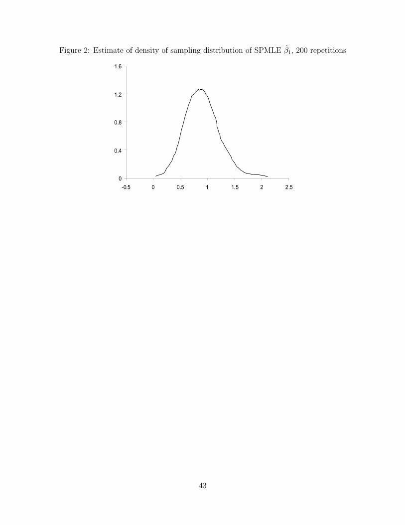
Figure 2: Estimate of density of sampling distribution of SPMLE β1, 200 repetitions

43

Figure 3: Density estimates log benefits in SIPP and QC

44

Figure 4: Estimate of density of the measurement error with smoothing parameter T = .7

45

Figure 5: Empirical hazard rate of welfare durations in SIPP

46

Tab

le1:

Sim

ula

tion

resu

lts

Pro

bit

model

:n

=50

0,n

1=

600,

num

ber

ofre

pet

itio

ns

200.

β1

β2

β0

σ2 ε

σ2 x∗

=1.

96a

Root

MSE

Mea

nbia

sStd

.dev

.R

oot

MSE

Mea

nbia

sStd

.dev

.R

oot

MSE

Mea

nbia

sStd

.dev

.

Ignor

ing

mea

s.er

ror

0.69

09-0

.687

1*0.

0730

0.14

520.

0679

*0.

1283

0.06

92-0

.034

0*0.

0603

Tru

ex∗

0.14

640.

0221

*0.

1447

0.13

10-0

.014

30.

1302

0.05

980.

0056

0.05

95K

now

nm

eas.

erro

rdis

t.0.

2862

0.03

300.

2843

0.14

98-0

.015

10.

1491

0.07

120.

0077

0.07

08M

argi

nal

info

rmat

ion

0.32

88-0

.092

30.

3156

0.18

86-0

.019

70.

1876

0.08

150.

0025

0.08

15

σ2 ε

σ2 x∗

=1b

Root

MSE

Mea

nbia

sStd

.dev

.R

oot

MSE

Mea

nbia

sStd

.dev

.R

oot

MSE

Mea

nbia

sStd

.dev

.

Ignor

ing

mea

s.er

ror

0.53

86-0

.531

1*0.

0894

0.15

460.

0562

*0.

1441

0.06

98-0

.017

7*0.

0675

Tru

ex∗

0.14

070.

0025

0.14

070.

1466

0.00

070.

1466

0.07

050.

0111

*0.

0696

Know

nm

eas.

erro

rdis

t.0.

2218

0.01

520.

2213

0.15

63-0

.004

60.

1563

0.07

580.

0135

*0.

0746

Mar

ginal

info

rmat

ion

0.24

810.

0082

0.24

800.

1701

-0.0

158

0.16

930.

0873

0.01

63*

0.08

58

σ2 ε

σ2 x∗

=.3

6cR

oot

MSE

Mea

nbia

sStd

.dev

.R

oot

MSE

Mea

nbia

sStd

.dev

.R

oot

MSE

Mea

nbia

sStd

.dev

.

Ignor

ing

mea

s.er

ror

0.29

38-0

.272

3*0.

1103

0.14

490.

0174

*0.

1439

0.06

30-0

.013

2*0.

0616

Tru

ex∗

0.13

840.

0123

0.13

790.

1477

-0.0

130

0.14

710.

0642

0.00

310.

0641

Know

nm

eas.

erro

rdis

t.0.

1711

0.03

36*

0.16

780.

1518

-0.0

177

0.15

070.

0655

0.00

420.

0653

Mar

ginal

info

rmat

ion

0.17

64-0

.032

5*0.

1733

0.17

43-0

.063

40.

1624

0.09

420.

0206

*0.

0919

aβ

1=

1,β

2=−

1,β

0=.5

;x∗∼N

(0,.

25),w∼N

(0,.

25),ε∼N

(0,σ

2 ε);

the

smoo

thin

gpa

ram

eter

sar

eT

=.7

for

the

dens

ity

ofε

andS

=T

=.6

for

the

join

tde

nsit

yofx∗ ,w

.bβ

1=

1,β

2=−

1,β

0=.5

;x∗∼N

(0,.

25),w∼N

(0,.

25),ε∼N

(0,σ

2 ε);

the

smoo

thin

gpa

ram

eter

sar

eT

=.6

for

the

dens

ity

ofε

andS

=T

=.7

for

the

join

tde

nsit

yofx∗ ,w

.cβ

1=

1,β

2=−

1,β

0=.5

;x∗∼N

(0,.

25),w∼N

(0,.

25),ε∼N

(0,σ

2 ε);

the

smoo

thin

gpa

ram

eter

sar

eT

=.7

5fo

rth

ede

nsit

yofε

andS

=T

=.2

for

the

join

tde

nsit

yofx∗ ,w

.

47

Table 2: Stationarity of distribution of nominal benefits in QC sample: Kruskal-Wallis test,n = 3318.

Kruskal-Wallis statistic Degrees of freedom p-value

Nominal benefits between months 57.2 50 0.2254Nominal benefits between years 6.1 4 0.1948

Table 3: Stationarity of distribution nominal benefit levels in QC sample: Kolmogorov-Smirnov test distribution in indicated month vs. the other months.

month # obs. K-S stat. p-value month # obs. K-S stat.10 p-value

1 82 0.077 0.725 27 80 0.078 0.7272 82 0.062 0.923 28 48 0.094 0.7933 75 0.105 0.391 29 67 0.120 0.3014 64 0.082 0.798 30 67 0.112 0.3835 67 0.106 0.455 31 63 0.096 0.6236 63 0.089 0.711 32 54 0.137 0.2737 58 0.127 0.319 33 62 0.091 0.6948 55 0.172** 0.082 34 87 0.073 0.7549 70 0.093 0.593 35 68 0.204* 0.00810 68 0.071 0.889 36 66 0.119 0.31711 68 0.120 0.293 37 68 0.136 0.16812 67 0.076 0.840 38 81 0.090 0.55113 69 0.142 0.132 39 62 0.146 0.15114 59 0.102 0.589 40 45 0.117 0.57315 61 0.123 0.329 41 72 0.057 0.97516 62 0.110 0.449 42 50 0.141 0.27917 57 0.103 0.594 43 61 0.137 0.20818 47 0.106 0.677 44 55 0.166 0.10119 59 0.074 0.905 45 68 0.113 0.36420 52 0.105 0.623 46 57 0.110 0.50721 43 0.109 0.694 47 63 0.088 0.72422 69 0.125 0.242 48 83 0.117 0.22123 70 0.041 1.000 49 80 0.140** 0.09224 69 0.128 0.220 50 62 0.081 0.82225 76 0.092 0.562 51 73 0.114 0.31226 64 0.138 0.180

∗ significant at 5% level∗∗ significant at 10% level

48

Table 4: Comparison of the distribution of welfare benefits in SIPP and QC samples.

Real benefits Nominal benefits

SIPP QC SIPP QC

Mean 285.3 303.8 304.2 327.7Std. Dev. 169.6 156.9 180.9 169.4Min 9.3 9.6 10 10Max 959 1598 1025 1801Skewness 1.08 1.27 1.07 1.33Kurtosis 4.60 6.83 4.54 7.46n 520 3318 520 3318Kolmogorov-Smirnov statistic .123 .128p-value .0000 .0000

Table 5: Descriptive statistics, n = 520.

Mean Std. Dev. Min Max

Welfare spell (month) 9.07 8.25 1 35Fraction censored 0.52 - 0 1Age (years) 31.8 8.2 18 54Disabled 0.84 - 0 1Labor hours per week 13.3 17.6 0 70Log real welfare benefits (week) 5.46 0.68 2.23 6.86Log nominal welfare benefits (week) 5.52 0.68 2.30 6.93Number of children under 18 1.92 1.02 1 7Number of children under 5 0.60 0.76 0 4Real non-benefits income ($1000/week) 0.234 0.402 0 0.360State unemployment rate (perc.) 6.72 1.41 2.9 10.9Education (years) 11.6 2.64 0 18

49

Table 6: Parameter estimates of duration model, n = 520, n1 = 3318.

MLE with marginal information MLE ignoring measurement error

Variable MLE Stand. Error MLE Stand. ErrorLog real benefits -0.3368 0.1025 -0.2528 0.0877Hours worked per week 0.2828 0.0955 0.2828 0.0938Real non-benefits inc. 0.1891 0.1425 0.1842 0.1527No. of children age < 5 -0.1855 0.1095 -0.1809 0.1111No. of children age < 18 0.0724 0.0674 0.0712 0.0718Years of education (/24) -0.1803 0.9877 -0.3086 0.9663Age (years/100) -0.0692 0.0505 -0.0691 0.0481State unempl. rate (perc.) 0.0112 0.0295 0.0082 0.0290Disabled -0.1093 0.1833 -0.1198 0.1867Baseline hazard (weeks)

1 0.0516 0.0097 0.0546 0.01052 0.0662 0.0120 0.0697 0.01273 0.0409 0.0097 0.0429 0.01044 0.1385 0.0203 0.1445 0.02115 0.0433 0.0121 0.0450 0.01286 0.0771 0.0169 0.0798 0.01777 0.0543 0.0151 0.0562 0.01568 0.0646 0.0180 0.0668 0.01869 0.0787 0.0211 0.0807 0.021710 0.0565 0.0189 0.0575 0.019511 0.0480 0.0184 0.0486 0.018612 0.0750 0.0250 0.0756 0.025213-14 0.0438 0.0146 0.0440 0.014415-16 0.0226 0.0113 0.0227 0.011417-18 0.0286 0.0143 0.0285 0.014319-20 0.0263 0.0152 0.0261 0.015021+ 0.0116 0.0058 0.0114 0.0055

The smoothing parameters are: distribution ε, T = .7, distribution of x∗, w, S = .875 and T = .9.

50