Nonlinear Estimation Techniques for Navigation - NATO Educational Notes/STO-EN... · Nonlinear Estimation Techniques for Navigation ... applying linear theory to nonlinear problems

Nonlinear Estimation Techniques for Navigation

Michael J. VethVeth Research Associates, LLC

Niceville, FL 32578USA

[email protected]

ABSTRACT

Optimal estimation techniques have revolutionized the integration of multiple sensors for navigationapplications. These estimation techniques typically make assumptions about the sensor measurements, namelythe sensor measurements and errors are well modeled as linear, Gaussian systems. Unfortunately, there is alarge class of potential navigation sources which are non-linear, non-Gaussian or both. This motivates thedevelopment and exploration of nonlinear estimation techniques suitable for integrated navigation systems.

This paper presents an overview of estimation techniques suitable for systems with nonlinearities which are notwell-suited to traditional linear or extended Kalman filter algorithms. The paper begins with a description ofthe generalized recursive estimation problem and associated notation and conventions. Next, the limitations ofapplying linear theory to nonlinear problems are addressed, along with techniques for compensating for theseadverse effects, including a brief overview of the traditional extended Kalman filter. In addition, themathematical effects of system nonlinearities on random processes are presented along with computationaltechniques for efficiently capturing this information, which serves as the foundation for the development of manynonlinear estimators. Next, the unscented Kalman filter (UKF) and particle filters (PF) are presented andanalyzed. Common limitations of nonlinear estimators are addressed and hybrid solutions are discussed. Thepaper concludes with a discussion and qualitative comparison of the strengths and weaknesses of variousrecursive estimation techniques from linear Kalman filtering to particle filtering, and their applicability tovarious problem spaces related to military navigation requirements.

STO-EN-SET-197 5 - 1

1.0 INTRODUCTION AND BACKGROUND

Military leaders have long understood the need for reliable, accurate navigation information. The ability toanswer the simple question of “Where am I?” is fundamental to the classical Clausewitzean principles ofoffensive, maneuver, economy of force, and mass. As such, nations have invested significant resources into thedevelopment of robust navigation solutions.

In order to be effective, navigation systems must be designed to meet mission requirements in four primaryareas: accuracy, integrity, continuity, and availability. Accuracy is the ability of the system to estimation positionand/or orientation relative to the true values. Integrity is the ability of the system to identify when accuracy isnot meeting desired levels. Continuity is a measure of the system’s capability to provide uninterrupted, qualitymeasurements. Availability is the overall percentage of time the system is able to provide accurate navigationinformation. Meeting all of these requirements can be very challenging, depending on the mission.

There are two primary decisions a navigation system designer must make in order to meet performancespecifications, namely, which (and what number of) sensors to use and how to integrate the sensors into onesolution. One common example is using updates from a Global Positioning System (GPS) receiver to aid aninertial navigation unit via a Kalman filter algorithm. In many cases, additional complementary sensors can beadded to improve the system robustness including: radar measurements, Doppler velocity sensors, barometricaltimeters, sonar, and celestial navigation sensors, to name a few.

The continually increasing requirements for cooperative engagement in dense urban environments and in areaswhere global navigation satellite system (GNSS) coverage is degraded or denied has spurned the development ofnovel navigation sensors. Some examples of these include: optical aiding, laser scanners, magnetic field sensors,acoustic sensors, pedometry, etc. Many of these sensors utilize signals of opportunity, i.e., signals not designedfor navigation. As a result, these sensors tend to have nonlinear error statistics.

While the standard Kalman filter works very well when system errors are well-described by Gaussianprobability density functions (pdf), the algorithm can suffer performance degradation or failure when theseassumptions are not met. This paper will focus on alternative recursive estimation algorithms that are able toaddress nonlinear and non-Gaussian navigation problems. The article is arranged as follows. First, a basicoverview of the stochastic estimation problem is presented along with the background of the linear Kalman filter.Next, the discussion is expanded to include nonlinear stochastic system models which sets the stage for thediscussion of nonlinear estimators. Finally, three classes of nonlinear estimators are presented including:Multiple Model Adaptive Estimators (MMAE), Unscented Kalman Filters (UKF), and particle filters (PF).Conclusions are drawn regarding strengths and weaknesses of the various classes of nonlinear estimators.

2.0 BACKGROUND ON STOCHASTIC ESTIMATION

The foundation of estimation theory is the development of a stochastic model for a given system of interest.This is motivated by the observation that most real-world systems experience some degree of randombehavior [1]. Sensors never make perfect measurements. Manufacturing variances cause random variation inthe performance of components. Even if a system could be created perfectly, it must still interact withuncontrollable, random disturbances in the environment. Fortunately, stochastic models can be developed thattreat these unknowns in a statistically-rigorous manner.


5 - 2 STO-EN-SET-197

A typical recursive estimation algorithm consists of two distinct operations: propagation through time andmeasurement updates. The estimator is tasked with maintaining an estimate of the state pdf conditioned on thecollection of measurements. A sample sequence from time k-1 to time k is

(1)

where is the system state vector and is the collection of observations given by

(2)

2.1 Linear Stochastic Systems

A typical linear system model consists of both a dynamic model and a model of the measurement devices. Thedynamics model can be expressed as a linear stochastic difference equation given by

(3)

where is the state vector at time k, is the state transition matrix at time k-1, is the state vector attime k-1, is the control influence matrix at time k-1, and is the control vector at time k-1, and is a random vector representing the uncertainty in the dynamics model. The additive noise vector is zero-meanand Gaussian with

(4)

where is the expectation operator, is the process noise covariance matrix and is the Kronecker deltafunction.

The measurement model can be expressed as:

(5)

where is the observation vector, is the observation matrix, and is a random vector representing theuncertainty in the measurement model. The measurement noise vector is zero-mean and Gaussian with

(6)

where is the measurement noise covariance matrix.

In the most general case, the probability density function (pdf) of the state vector, conditioned on the priormeasurements, provides all possible statistics that could be used to develop a state estimate. The conditional pdfis given by

(7)

where represents the collection of observations up to, and including, time k. This is also knownas the a posteriori state pdf. An example of a typical Kalman filter application is shown in Figure 1.



2.2 Linear Kalman Filter

The a posteriori pdf is guaranteed to be Gaussian under the following conditions:

• The system dynamics and measurement components consist exclusively of linear models• The system and measurement noises are white and Gaussian• All initial conditions can be represented as Gaussian random variables

In this case, the entire statistics of the pdfs of interest can be expressed as a mean vector and covariance matrix.This unique property is exploited by the linear Kalman filter.

The Kalman filter has two distinct steps: propagation of the mean and covariance between time epochs (i.e.,propagation), and incorporating a discrete observation (i.e., update). Given the linear stochastic system modeldriven by white Gaussian noise sources shown in (3) and (5), the Kalman filter propagation equations are givenby

(8)and

(9)

Figure 1. Typical Kalman Filter Application. The estimator produces an optimal estimate of thesystem state based on observed measurements and known control inputs.



where is the a priori state estimate at time k, is the state transition matrix at time k-1, is the aposteriori state estimate at time k-1, is the a priori state covariance matrix at time k, is the aposteriori state covariance matrix at time k-1, and is the process noise covariance matrix at time k-1.

The Kalman filter measurement update equations are:

(10)

and

(11)

The Kalman gain, , is

(12)

The linear Kalman filter algorithm is optimal by every conceivable measure, is easily implemented on a digitalcomputer, and has served as the benchmark standard of recursive estimation algorithms for decades [4].

2.3 Effects of Nonlinearities on the Linear Kalman Filter

While many systems are well-modeled by linear stochastic equations, most real-world applications are nonlinearat some level. There are many types of nonlinearities to consider. Some examples include non-Gaussian noisesources, saturation effects, nonlinear dynamics or measurement models, and jump discontinuities. All of theseeffects ultimately result in the true conditional state pdfs being non-Gaussian in nature, which violates thefundamental assumptions of the linear Kalman filter [3].

If the degree of nonlinearity is relatively small, the extended Kalman filter (EKF) can provide acceptableresults [3]. The EKF filter design is based on linearization of the system and measurement models using a first-order Taylor series expansion.

Although the EKF is very widely used in navigation applications, there are limitations that should be understood.First, the EKF is subject to linearization errors. These linearization errors result in incorrect state estimates andcovariance estimates and can lead to unstable operation, known as filter divergence. EKFs can be extremelysensitive to this effect during periods of relatively high state uncertainty such as initialization and start-up. Thesecond issue is the inherently unimodal assumption of the EKF. In cases where multi-modal densities are knownto exist, the EKF would not be a good choice.

In the following sections, various types of nonlinear estimation approaches will be addressed. Each approachwill be presented along with a typical navigation application. The first approach to address non-Gaussiandensities is the class of Gaussian Sum Filters, namely the Multiple Model Adaptive Estimation technique.

2.4 Multiple Model Adaptive Estimation (MMAE)

The Multiple Model Adaptive Estimation (MMAE) filter extends the linear Kalman filter to address the situationof unknown or uncertain parameters in the system model. MMAE is in the class of estimators known as



Gaussian Sum Filters. Others in the class include the Interacting Multiple Model (IMM) filter and the Rao-Blackwell particle filter. Some examples of applications that fall into this category include: system failuremodes, unknown structural parameters, “jump” processes, etc. [3].

The MMAE filter represents the state pdf using a sum of individually-weighted Gaussian densities. This allowsthe filter to properly account for complex, non-Gaussian densities. In this way, the effects of the uncertainparameters on the overall state pdf are explicitly and directly maintained inside the estimator. An example of asum of Gaussian density is shown in Figure 2.

Consider the system represented by the linear stochastic difference equation (3)

(13)

and corresponding measurement equation (5)

(14)

Figure 2: Example Sum of Gaussian Density. Gaussian sums can be used torepresent a wide variety of densities, including multi-modal densities as shown in

this example.



which are repeated here for clarity. Similarly, the noise sources, and , are zero-mean and Gaussian withcovariances

(15)

and

(16)

respectively.

In contrast to the standard linear Kalman filter, consider the additional situation where a portion of the systemmodel parameters are unknown. These unknowns could be in the structure of the dynamics model (i.e., , ),in the structure of the measurement model (i.e., ), or in the statistics of the uncertainties (i.e., , ). Someexamples of applications with these uncertainties include: systems with unknown or dynamic sensor biases orscale factors, system with changing operating conditions that affect the linearized model, and trackingapplications where the characteristics of the target are unknown.

The estimation problem becomes that of a dual estimator. In other words, the unknown parameters must beincluded in the unknowns. The MMAE estimator derivation proceeds by defining a new random vector, , thatcontains the unknown parameters. The a posteriori pdf is augmented to create a new, joint a posteriori pdf ofinterest

(17)

where is the system state vector and is the collection of observations given by

(18)

Equation (17) can be rewritten using Bayes' rule as

(19)

Assuming the parameter vector is of finite dimension (i.e., ) the parameter density can be expressed as

(20)

Invoking Bayes' rule once again yields

(21)

Finally, invoking Bayes' rule on the numerator and expressing the denominator as equivalent integral of themarginal density on gives the following relation

(22)



It should be noted that the term is the measurement prediction density conditioned on a knownparameter vector and all prior measurements. Given the system model from (13) and (14), this pdf is given bythe following Gaussian density

(23)

where is the residual covariance given by

(24)

Finally, the term is the a priori density of the parameter vector. Unfortunately, the integral in thedenominator of (22) is intractable in general. However, if the system parameters can be chosen from a finite set,

i.e., then the parameter density can be expressed as the sum of the individual

probabilities of the finite set

(25)

where is the probability weight of the j-th parameter vector, .

Substituting (25) into (22) yields

(26)

Because the probability weights are independent of the integration, the order of integration can be reversedwhich results in

(27)

which can be further reduced using the sifting property on the denominator



(28)

The j-th probability weighting at time k can be defined as the following recursive relationship

(29)

In a similar fashion to (23), the term is the measurement prediction density based on the j-th model. This pdf is given by the following Gaussian density

(30)

where is the measurement realization at time k, is the j-th observation matrix at time k, is the j-th a

priori state estimate, and is the j-th residual covariance. Once a measurement is realized, the j-thmeasurement likelihood (30) can be directly evaluated and the associated weight scaled.

Substituting (29) into (28) yields an updated expression of the a posteriori pdf

(31)

Substituting (31) into (19)

(32)

and finally using the sifting property of the delta function yields a tractable expression for the a posteriori pdf

(33)

which, given the linear, stochastic system model given in (13) and (14) is simply the weighted sum of the outputof J Kalman filters, each based on the parameter vector . This can be visualized as a bank of J independentKalman filters as shown in Figure 3.



The blended state estimate and covariance is given by

(34)

and

(35)

respectively.

The MMAE filter operating sequence is as follows. When an observation is made, the residual likelihood isevaluated for each filter and the corresponding model weight is scaled appropriately. Models that agree wellwith the residual sequence will be increased in weight. Models that do not agree with the residual sequence willdecrease in weight.

Figure 3: Typical MMAE block diagram. The MMAE estimator consists of a bank of independentKalman filters, each based on a discrete parameter vector.


5 - 10 STO-EN-SET-197

2.6 Unscented Kalman Filter

As discussed previously, the recursive estimation problem is fundamentally concerned with estimating theconditional state density. When dynamic or measurement models are nonlinear, the linear, Gaussianassumptions of the linear Kalman filter are invalidated. The extended Kalman filter exploits a first-order Taylorseries expansion to approximate the transformation of random vectors through the nonlinearity. Unfortunately,this first-order technique can fail when nonlinearities become large. In addition, the first-order Taylor seriesmethod requires calculation of a Jacobian matrix which is unnecessary in the unscented and particle filteralgorithms.

The Unscented Kalman Filter (UKF) exploits the Unscented Transform (UT) to transform random vectorsthrough nonlinearities. For Gaussian random variables, the UT captures the correct statistics equivalent to athird-order Taylor series [7]. In addition, the UT is computationally efficient compared to particle filteringalgorithms.

2.6.1 Unscented Transform

The unscented transform represents a random vector's density as a collection of carefully-chosen “sigma points.”The sigma points are chosen so that they can be directly transformed through a nonlinear (or linear) functionwhile more accurately maintaining the statistics of true density. Consider the following generalizedtransformation, where is a random vector with dimension , is a random vector with dimension

, and is a mapping function from . The mean and covariance of is given by

(36)

and

(37)

respectively.

The first step of the forward unscented transform is to calculate the collection of sigma points, , which is adeterministic function of and . The sigma point matrix consists of sigma points, , given by

(38)

with the subscript notation representing the column number (e.g., is the j-th column of the matrix ), and is the Cholesky square root. The scaling parameter, , is given by

(39)


STO-EN-SET-197 5 - 11

The sigma point weights are given by the collection

(40)

The scalars , , and are tuning parameters that vary the spread of the sigma points. Default values forGaussian densities are , , .

Given a collection of sigma points, the mean and covariance of the random vector is calculated via

(41)

and is referred to as the reverse unscented transform.

A transformation of random variable (e.g., ) is accomplished by simply passing each sigma point of ,namely , through the mapping function

(42)

to produce a transformed collection of sigma points, . Each sigma point has dimension , as given by themapping function . The mean and covariance of can be recovered using the same procedure given in (41),namely

(43)

In the next section, the unscented transform will be used as the basis for a recursive estimation algorithm knownas the Unscented Kalman Filter (UKF).


5 - 12 STO-EN-SET-197

2.6.2 Unscented Kalman Filter

The UKF algorithm is conceptually similar to the linear Kalman filter. There are two distinct steps: propagationof the state vector density over time, and updating the state vector density based on a measurement observation.

Consider the nonlinear stochastic system model given by

(44)

where the process noise, , and measurement noise, , are both zero-mean, independent, white Gaussianrandom vectors with covariance and , respectively. In addition, assume the a posteriori state estimate andcovariance is available at time k-1, (i.e., and ).

The first step is to propagate the state vector from time k-1 to time k. This is accomplished using the forwardunscented transform to create sigma points at time k-1, represented by . The sigma points are transformedthrough the nonlinear system state transition function

(45)

The mean and covariance of are calculated using the backward unscented transform and the effects of theprocess noise are incorporated to produce the a priori state estimate and covariance at time k

(46)

A block diagram of the UKF propagation algorithm is shown in Figure 4.


STO-EN-SET-197 5 - 13

The measurement update proceeds similarly, beginning with the transformation of the a priori mean andcovariance into a collection of sigma points, . These sigma points are transformed into the measurementspace via

(47)

The measurement mean, , covariance, , and cross-correlation matrix, are calculated as

(48)

Finally, the a posteriori statistics are calculated using the standard Kalman update algorithms, albeit in a slightlydifferent, but mathematically equivalent, form. The Kalman gain is given by

(49)

Figure 4: Unscented Kalman Filter Propagation.


5 - 14 STO-EN-SET-197

and the state estimate and covariance are given by

(50)

A block diagram of the UKF measurement update process is shown in Figure 5.

In addition to the above algorithm, other UKF algorithms exist to address the case of non-additive noise sources.The reader is referred to the literature [2],[5] for more details.

As mentioned previously, the UKF has some important advantages over the linear or extended Kalman filter.First, the UKF algorithm captures higher order statistics than the linear or extended Kalman filter. In addition,the requirement to calculate Jacobians is completely eliminated resulting in less chance of errors, especially forcomplicated models. However, there are some disadvantages of the UKF that need to be considered. First, theUKF requires slightly more processing time than the equivalent EKF. Finally, the UKF is still unable to capturethe statistics of multi-modal densities.

2.7 Particle Filter

The class of recursive estimators known as particle filters utilize a different approach for representing the statepdf, which has the potential to accurately maintain the statistics of interest at an arbitrary level. Two mainclasses of particle filter exist: grid-based or discrete methods, and continuous methods. Due to space limitations,only the grid-based particle filter algorithm will be developed in this article. For additional information on othertypes of particle filters, the reader is referred to [5].

Figure 5: Unscented Kalman Filter Measurement Update.


STO-EN-SET-197 5 - 15

2.7.1 Propagation

The propagation of the state pdf through time incorporates the stochastic effects of the system model. Thisrequires knowledge of the transition pdf. To accomplish this mathematically, the property of densitymarginalization is required. Recall the marginalization integral

(51)

Substituting our a priori density at time k for and the a posteriori density at time k-1 for yields

(52)

where is the transition density. Because we assume a first-order Markovian system model,the transition density is independent of the measurement observations, thus

(53)

Substituting (53) into (52) yields the well-known Chapman-Kolmogorov equation

(54)

2.7.2 Measurement Update

The measurement update incorporates the state knowledge gained during the observation by exploiting themeasurement model. The measurement update is derived by recalling Bayes' rule

(55)

The derivation begins by separating the current measurement from the measurement collection in the aposteriori pdf

(56)

Applying Bayes' rule to the right-hand side of (56) yields

(57)


5 - 16 STO-EN-SET-197

Because the conditional observation is density is independent of the prior observations, the followingsimplification can be applied

(58)

Substituting (58) into (57) yields the measurement update equation

(59)

where is the measurement likelihood, and is referred to as the evidence. The evidenceeffectively serves as a normalization factor to ensure unit area of the a posteriori pdf. As a final note, applyingthe marginalization integral to the evidence yields an equivalent form that will aid our development of theparticle filtering algorithms

(60)

2.8 Discrete Particle Filtering Algorithm

The discrete particle filter is conditioned on the assumption of partitioning the state space into a finite set ofdiscrete states. A discrete random variable is characterized by the probability mass function (pmf). The pmfconsists of a collection of states and corresponding probability weights. The sum of all weights must equal one.

The delta function can be used to create a mathematical representation of a pmf, for example

(61)

where is the probability weight for particle j, and is the discrete state location of particle j. Thus, the aposteriori state pmf is given by

(62)

where represents the probability weight for particle j at time k-1, conditioned on measurements up-to,

and including, time k-1.

2.8.1 Propagation Relations

Because the discrete states are at fixed locations, only the particle weights change as an effect of propagation andmeasurement updates. The propagation weighting function is derived using the Chapman-KolmogorovEquation, presented in the previous section. Substituting the a posteriori pmf into (54) yields


STO-EN-SET-197 5 - 17

(63)

Changing the order of integration and simplifying using the sifting property gives

(64)

Because the state vector is discrete, the transition density can be expressed as

(65)

Substituting (65) into (64) and grouping terms

(66)

The bracketed term represents the particle weights that have been updated by the transition probability (i.e., apriori particle weights). Using the notation presented previously, the a priori particle weights are formally givenby

(67)

and the corresponding pmf is given by

(68)

2.8.2 Measurement Update

The measurement update weighting function is determined by substituting the a priori pmf (68) and (60)into (59)

(69)


5 - 18 STO-EN-SET-197

Applying the sifting property and simplifying yields

(70)

Grouping the weighting terms and expressing using the notation presented previously results in

(71)

with the j-th a posteriori particle weight given by

(72)

3.0 EXAMPLE APPLICATION

Consider the following two-dimensional vehicle navigation scenario shown in Figure 6. The vehicle is equippedwith a sensor that receives an RF, carrier-phase ranging signal from a constellation of transmitters. Thetransmitters are positioned in circular orbits around the area of interest. For simplicity, time synchronization isassumed between all devices.


STO-EN-SET-197 5 - 19

The vehicle moves at a known, constant velocity. The heading can be represented as a first-order Gauss-Markov(FOGM) process. Thus, the vehicle stochastic dynamics model can be expressed as

(73)

where and are the x-position and y-position at time , respectively, is the heading, is the vehiclespeed, is the sampling interval, is the FOGM heading time constant, and is the process noise. Theprocess noise is a zero-mean, Gaussian process with

(74)

where is the variance of the FOGM heading process, and is the Kronecker delta function.

The measurement equation for transmitter a is given by

(75)

where and are the x and y locations of transmitter a at time k, respectively. The carrier phase cyclenumber is represented by the integer with wavelength given by . Finally, the measurement noise is

Figure 6: Simple Navigation Scenario. The transmitters orbit the area of interest while broadcastinga navigation signal.


5 - 20 STO-EN-SET-197

represented by the zero-mean, Gaussian random variable with variance kernel

(76)

3.1 Monte Carlo Analysis

The scenario outlined in the previous section is used to evaluate the performance of the extended Kalman filter,unscented Kalman filter, multiple-model adaptive estimator, and particle filter. Six scenarios are chosen todemonstrate the strengths and weaknesses of the various algorithms. For each scenario, a 30-run Monte Carlosimulation is performed. Each filter is executed using identical input data and the results for estimation error arecompared.

The scenarios are evaluated for two main cases: known and unknown integer cycle count. When the integercycle count is known, the state estimate is unimodal and appropriate for the EKF, UKF, and particle filter. Whenthe integer cycle count is unknown, only the MMAE and particle filter are evaluated as the EKF and UKF wouldrequire modifications to address integer ambiguity resolution methods.

The radius and number of transmitters is varied in order to change the level of nonlinearity and observability ofthe system. The scenarios are arranged in general order of difficulty and are listed in Table 1. The vehiclemotion parameters are the same for all scenarios with m/s, s, and deg.

Table 1: Transmitter characteristics for UAV navigation scenario example.

Scenario

Initial StateUncertainty

Standard DeviationNumber of

Transmitters

Transmitter Range(X, Y, Z)

TransmitterGeometry

TransmitterMeasurement

StandardDeviation

( )

TransmitterWavelength

( )

1 5 m 5 m 25 deg 3 1000 m Excellent 0.2 m 1 m

2 5 m 5 m 25 deg 3 10 m Excellent 0.2 m 1 m

3 5 m 5 m 25 deg 2 10 m Good 0.2 m 1 m

4 5 m 5 m 25 deg 2 10 m Poor 0.2 m 1 m

5 5 m 5 m 25 deg 1 1000 m Very Poor 0.2 m 1 m

6 5 m 5 m 25 deg 1 10 m Very Poor 0.2 m 1 m

3.1.1 Known Integer Ambiguity

In the case where the integer cycle number is known, the problem is reduced to a simple problem ofmultilateration. As the transmitter range is decreased, the observation becomes more nonlinear. Thesenonlinearities are exacerbated as the transmitter geometry results in reduced observability. The ensemble root-mean-square (RMS) error and estimator quality histograms for each scenario are shown in Figures 7 – 12.


STO-EN-SET-197 5 - 21

Scenario 1 is the least challenging case as the three, well-separated transmitters provide excellent observabilityand their long range from the vehicle reduce the nonlinearity to a very low level. As expected, all of theestimators demonstrate consistent and accurate performance for this scenario. The consistency of the filter is ameasure of the a posteriori state estimate errors relative to the filter predicted a posteriori standard deviation. Ina well-tuned filter, the error statistics will be consistent with the filter predicted uncertainty. A filter that is notconsistent is reporting an inaccurate confidence and is not operating optimally. In addition, the filter issusceptible to divergence. The next scenario reduces the satellite radius from 1000 meters to 10 meters in aneffort to introduce some nonlinear measurements.

Figure 7: Estimator errors and consistency histograms for Monte Carlo Scenario 1. In this case, allfilters provide accurate, consistent results.


5 - 22 STO-EN-SET-197

In Scenario 2, shown in Figure 8,the increase in measurement nonlinearity is evidenced by an increase in errorsfor the EKF and UKF, especially during the first few seconds of operation. After the initialization period, boththe EKF and UKF converge to performance similar to the particle filter. In addition, the EKF's error estimateshows signs of overconfidence as shown by the increase in the tails of the error ratio deviations. It is interestingto note that while the UKF shows almost identical estimation errors to the EKF, the UKF does maintain a moreaccurate filter covariance. This is one of the benefits of the UKF. In the next scenario, the number oftransmitters is reduced from three to two.

Figure 8: Estimator errors and consistency histograms for Monte Carlo Scenario 2. In this case, allfilters provide accurate, consistent results, although the particle filter demonstrates slightly better

accuracy and consistency.


STO-EN-SET-197 5 - 23

In Figure 9, the results of Scenario 3 are shown. The reduction in transmitter observability results in a reductionin accuracy for all filters, although the EKF and UKF show the greatest increase in errors. Additionally, theconsistency of both the EKF and UKF are reduced as shown by the increase in the histogram tails.

Figure 9: Estimator errors and consistency histograms for Monte Carlo Scenario 3. The particlefilter is producing a more accurate result than the EKF and UKF. In addition, the EKF's error

estimates are beginning to become overly optimistic.


5 - 24 STO-EN-SET-197

The results for Scenario 4 are shown in Figure 10. This scenario continues to reduce the observability of thetransmitters by reducing the angular separation. As seen in the figure, the EKF is demonstrating clear signs ofinconsistency via a markedly overconfident filter. As mentioned previously, this can lead to filter divergence.

Figure 10: Estimator errors and consistency histograms for Monte Carlo Scenario 4. Similar to theScenario 3, the particle filter is producing a more accurate result than the EKF and UKF. Both the

UKF and EKF's error estimates are overly optimistic.


STO-EN-SET-197 5 - 25

Scenario 5 is a single satellite scenario with relatively low measurement nonlinearities. In this case, all filtersshow good accuracy. The EKF shows some signs of inconsistent operation, however they are relatively small.Overall, each filter handles this scenario well. In the next scenario, the nonlinearities will be increased.

Figure 11: Estimator errors and consistency histograms for Monte Carlo Scenario 5. In thisscenario, the filters perform similarly due to the relatively low level of nonlinearity.


5 - 26 STO-EN-SET-197

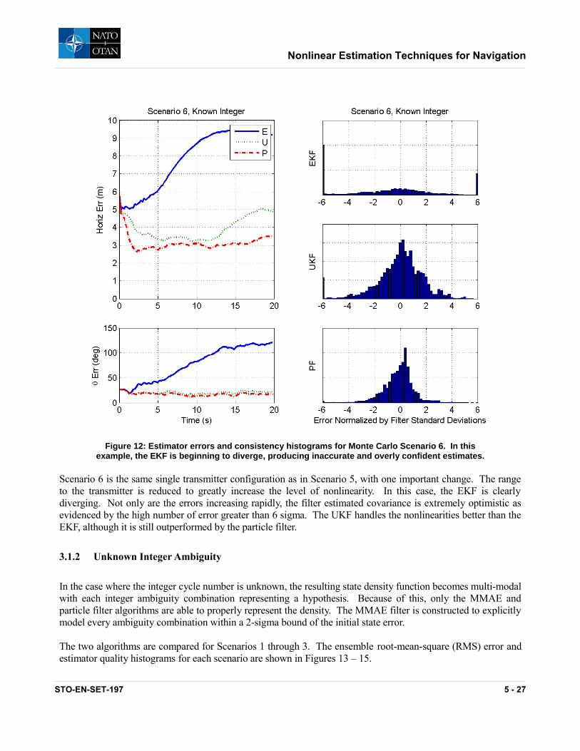
Scenario 6 is the same single transmitter configuration as in Scenario 5, with one important change. The rangeto the transmitter is reduced to greatly increase the level of nonlinearity. In this case, the EKF is clearlydiverging. Not only are the errors increasing rapidly, the filter estimated covariance is extremely optimistic asevidenced by the high number of error greater than 6 sigma. The UKF handles the nonlinearities better than theEKF, although it is still outperformed by the particle filter.

3.1.2 Unknown Integer Ambiguity

In the case where the integer cycle number is unknown, the resulting state density function becomes multi-modalwith each integer ambiguity combination representing a hypothesis. Because of this, only the MMAE andparticle filter algorithms are able to properly represent the density. The MMAE filter is constructed to explicitlymodel every ambiguity combination within a 2-sigma bound of the initial state error.

The two algorithms are compared for Scenarios 1 through 3. The ensemble root-mean-square (RMS) error andestimator quality histograms for each scenario are shown in Figures 13 – 15.

Figure 12: Estimator errors and consistency histograms for Monte Carlo Scenario 6. In thisexample, the EKF is beginning to diverge, producing inaccurate and overly confident estimates.


STO-EN-SET-197 5 - 27

Scenario 1 combines nearly linear measurements with an overdetermined number of satellites in an excellentgeometric configuration (i.e., highly observable state). As such, both estimators converge to an accuratesolution. There is some inconsistency observed in the MMAE error ratios, however this is likely due to theselection of the initial ambiguity hypothesis bound which has the effect of making the MMAE algorithm slightlyoverconfident. In the next scenario, the transmitter range will be reduced which increases the measurementnonlinearity.

Figure 13: Estimator errors and consistency histograms for Monte Carlo Scenario 1. In thisexample, both the MMAE and particle filter are able to converge to an accurate state estimate.


5 - 28 STO-EN-SET-197

Scenario 2 increases the nonlinearity of the observations by reducing the transmitter range. Both estimators arestill able to converge to an accurate solution. As a result of the nonlinearities, however, the MMAE algorithm'sfilter uncertainty is slightly optimistic as seen by the increase in the tails of the normalized error ratios.

Figure 14: Estimator errors and consistency histograms for Monte Carlo Scenario 2. Bothestimators converge to an accurate solution, however the uncertainty for the MMAE algorithm is

beginning to show signs of inconsistency.


STO-EN-SET-197 5 - 29

Scenario 3 maintains the measurement nonlinearity of Scenario 2, but reduces the number of transmitters fromthree to two. In this case, the MMAE algorithm is unable to converge to an accurate solution while the particlefilter seems unaffected.

In the remaining scenarios (4 through 7), both estimators fail to converge to an accurate solution during thesimulation time. The general trend of the consistency results remain the same, i.e., the MMAE algorithm showsa decrease in consistency when the nonlinearities increase.

In the next section, the computational burden of each algorithm is presented.

3.1.3 Processing Time Analysis

The nonlinear estimation algorithms presented in this article require varying levels of processing time. In theexample, the algorithms were implemented in Matlab and all Monte Carlo simulations were timed to provide arough measure of comparison. None of the algorithms were optimized or vectorized. The processing timeresults are shown in Table 2. All times are normalized to the time expended by the EKF algorithm.

Figure 15: Estimator errors and consistency histograms for Monte Carlo Scenario 3. In thisexample, the particle filter is able to converge to an accurate solution while the MMAE algorithm is

unsuccessful.


5 - 30 STO-EN-SET-197

EKF UKFMMAE

(1 transmitter,21 hypotheses)

MMAE(2 transmitters,441 hypotheses)

MMAE (3 transmitters,

9261 hypotheses)

Grid ParticleFilter

(~1.2 M cells)

Normalized Time(relative to EKF)

1 ~1 7 15 400x 425x

Table 2: Comparison of processing time for various nonlinear estimation algorithms.

The results clearly show the computational burden of the particle filter and the MMAE filter as the number ofhypotheses becomes large. One of the known drawbacks of particle filtering methods is computationalcomplexity, especially in high dimensional state spaces. Optimization and parallelization techniques havedemonstrated substantial improvements in processing time for particle filters. The significant computationalburden of high-dimensional particle filters is a considerable drawback for real time environments.

4.0 CONCLUSIONS AND DISCUSSION

In this article, the foundations of nonlinear estimation theory is presented along with a number of nonlinearestimation algorithms. The ability of each algorithm to properly model the effects of various types ofnonlinearities is shown by analysis and via a simple example. The results show that as the nonlinearities areincreased, both the accuracy and consistency of the EKF are decreased. This is a well-known issue with theEKF and is one of the main reasons to choose a more advanced nonlinear estimator when moderatenonlinearities are expected.

For random vectors with unimodal densities, the UKF is a compelling choice. In all cases shown in the testscenarios, the UKF shows equal or better accuracy than the EKF. Moreover, the UKF maintains a much moreconsistent state covariance estimate. The importance of consistency cannot be overemphasized. The ability ofan estimator to produce an accurate estimate of the quality of its performance is a key component in a systemwith integrity requirements. In addition, the UKF does not require significantly more processing resources thanthe EKF.

Given unlimited computational resources, the particle filter would always give the most accurate estimationperformance. Unfortunately, this is oftentimes impractical, especially for high-dimensional state vectors. In thesimplest construction, the memory and processing requirements rise geometrically with the number of states.This can quickly become untenable. To compensate for this known limitation a number of different particlefiltering strategies have been presented in the literature [5],[6],[2]. The general approach is to focus the particlesonly in the areas of highest likelihood, thus maintaining the important modes of the density with a minimum ofresources. This is currently an area of active research.

For military navigation systems, integrity and accuracy are paramount. While this application area has beendominated by the EKF to this point, the advent of non-traditional aiding sources motivates a more advancedfilter. The UKF is well-suited to meet future needs due to its demonstrated ability to accurately and consistentlywork with low-to-medium nonlinearities while maintaining an acceptable computational burden.


STO-EN-SET-197 5 - 31

5.0 BIBLIOGRAPHY

1. Brown, Grover and Patrick Hwang, Introduction to Random Signals and Applied Kalman Filtering.New York: John Wiley & Sons, 1997.

2. Julier, S.J. and Uhlmann, J.K., "Unscented Filtering and Nonlinear Estimation". Transactions of theIEEE, 92(3):401 - 422, 2004.

3. Maybeck, Peter S., Stochastic Models, Estimation, and Control Volume II. Orlando, FL: AcademicPress, Inc., 1979.

4. Maybeck, Peter S., Stochastic Models Estimation and Control, Volume 1. Orlando, FL: Academic Press,Inc., 1979.

5. Ristic, Branko and Sanjeev Arulampalam and Neil Gordon, Beyond the Kalman Filter: Particle Filtersfor Tracking Applications. Artech House, 2004.

6. Van Der Merwe, R. and Doucet, A. and De Freitas, N. and Wan, E., "The Unscented Particle Filter".Advances in Neural Information Processing Systems, 584-590, 2001.

7. Wan, E.A. and Ven Der Merwe, R.. "The Unscented Kalman Filter for Nonlinear Estimation". AdaptiveSystems for Signal Processing, Communications, and Control Symposium 2000, 153-158, 2000.


5 - 32 STO-EN-SET-197

Documents

Nonlinear Estimation Techniques for Navigation - NATO Educational Notes/STO-EN... · Nonlinear Estimation Techniques for Navigation ... applying linear theory to nonlinear problems