Engineering with Computers (1999) 15: 73–89 1999 Springer-Verlag London Limited

Nonlinear Finite Element Analysis using an Object-OrientedPhilosophy – Application to Beam Elements and to the CosseratContinuum

E.N. Lages1, G.H. Paulino2, I.F.M. Menezes3 and R.R. Silva41Department of Structural Engineering, Universidade Federal de Alagoas (UFAL), Maceio´, AL, Brazil; 2Department of Civil &Environmental Engineering, and Graduate Group in Applied Mathematics (GGAM), University of California, Davis, CA, USA;3TeCGraf (Computer Graphics Technology Group), PUC-Rio, Rio de Janeiro, RJ, Brazil;4Department of Civil Engineering, PUC-Rio, Rio de Janeiro, RJ, Brazil

Abstract. An Object-Oriented Programming (OOP) frame-work is presented for solving nonlinear structural mechanicsproblems by means of the Finite Element Method (FEM).Emphasis is placed on engineering applications(geometrically nonlinear beam model, and elastoplasticCosserat continuum), and OOP is employed as an effectivetool, which plays an important role in the FEM treatmentof such applications. The implementation is based on compu-tational abstractions of both mathematical and physical con-cepts associated to structural mechanics problems involvinggeometrical and material nonlinearities. The overall classorganization for nonlinear mechanics modeling is discussedin detail. All the analyses rely on a generic control classwhere several classical and modern nonlinear solutionschemes are available. Examples which explore, demonstrateand validate the main features of the overall computationalsystem are presented and discussed.

Keywords. Beam elements; Cosserat continuum;Finite Element Analysis (FEA); Geometric nonlin-earity; Material nonlinearity; Nonlinear solutionschemes; Object-Oriented Programming (OOP);Structural mechanics

1. Introduction

Object-Oriented Programming (OOP) is a relativelynew philosophy of programming which aims atincreasing the overall quality of computational sys-tems. Computer codes that are written based onsuch a philosophy are easier to maintain and to

Correspondence and offprint requests to: Professor G. H. Paulino,Department of Civil and Environmental Engineering, Universityof Illinois, 2209 Newmark Laboratory, 205 N. Mathews Ave.,Urbana IL 61801-2352, U.S.A. Email: paulino@uiuc.edu

expand, reducing probability of errors due to pro-gramming. Moreover, by means of OOP concepts,new implementations can take place with no needto restructure the pre-existing code, and thus codereuse is maximized to a large extent. To achievethis level of development, however, a thoroughunderstanding of the whole methodology employedand an extensive effort in program organizationare required. Such efforts are demonstrated in thedevelopment of this work.

Compared to classical programming, OOPrequires a more intrinsic integration between theoryand numerical implementation. This integration isexplored here in engineering applications involvinggeometrically nonlinear analysis of frames discret-ized with beam elements, and materially nonlinearproblems considering the elastoplastic Cosserat con-tinuum. The main reason for choosing these twoapplications is because both models present the sameDegrees Of Freedom (DOF), although in differentsettings (discrete versus continuum, respectively).Moreover, according to Roux [1], the equations oftwo-dimensional (2D) network of beam elements area straightforward discretization of the equations ofa 2D Cosserat elastic medium.

The goal for the remainder of this paper consistsof developing a comprehensive presentation, and thenext sections are organized as follows. First, a briefliterature review is provided, and some backgroundon OOP is given where the basic terminology isestablished. Next, a ‘unified approach’ is discussedfor solution of nonlinear systems which arise in theFEM — the nonlinear solution process isaccomplished by means of a control class whereseveral solution schemes are available. Afterwards,geometrically (beam elements considering shear

74 E.N. Lageset al.

effects) and materially (elastoplastic Cosseratcontinuum) nonlinear problems are discussed withinan OOP framework. Subsequently, conclusions areinferred and directions for future research are dis-cussed.

2. Brief Literature Review

Preliminary ideas about OOP date back to the 1960s,with the development of theSimula language [2].As pointed out by Fenves [3], this language intro-duced the idea of a class which can create instancesthat respond to procedures in a similar manner.Based upon the ideas presented in theSimula langu-age, research was conducted at the Xerox Palo AltoResearch Center resulting in the first substantialinteractive, display-based implementation, called theSmalltalk-80 language [4], which provides a veryuniform application of the OOP paradigm [3,5].After the establishment of theSmalltalk language,several other languages became available, forexample, Flavors [6] (with the idea of multipleinheritance),Objective C[7] and C11 [8] (whichare extensions of the C language for objects).

The OOP technique has been widely used invarious applications, such as simulation programs,graphical user interfaces, and artificial intelligence(AI), just to mention a few of them. However,according to Zimmermann et al. [9], the applicationof OOP to the Finite Element Method (FEM) onlyappeared at the end of the last decade, with thework by Rehak and Baugh [10] and Forde et al.[11]. Zimmermann and co-authors [9,12–16] havepublished several interesting articles describing indetail the fundamental aspects relating applicationof OOP techniques to implementation of the FEM.For instance, Mene´trey and Zimmermann [17] haveapplied the concepts of OOP to the FEM for nonlin-ear static analysis, specifically toJ2 plasticity prob-lems. A detailed object-oriented implementation hasbeen presented, which includes the description of themain classes and methods for solving the nonlinearproblem. Mackie [18] has described the benefits thatcan be attained by applying OOP to Finite ElementAnalysis (FEA). The concepts of OOP are presenteddirectly in terms of the FEM. Alves Filho andDevloo [19] have discussed the basic aspects of theOOP philosophy, and its implementation in scientificcomputations, using the FEM as an example ofsuch implementation. Another example of an object-oriented finite element model has been presented byRaphael and Krishnamoorthy [20]. They have alsodiscussed the general concepts of OOP, together

with a detailed description of the main classes in afinite element model. Bettig and Han [21] havepresented an object-oriented framework for inter-active numerical analysis in a graphical user inter-face environment. Besson and Foerch [22] havediscussed aspects of object-oriented finite elementdesign that become relevant as the project sizeincreases. They have presented a detailed descriptionof the computational implementation issues, and alsoa very interesting comparison between performanceof the OOP implementation using C11, and anexisting FORTRAN implementation, with respect tothe Central Processing Unit (CPU) time, forobtaining the elastic and viscoplastic solutions of aplate problem. Recently, Jeremic´ and Sture [23]presented a programming tool which facilitatesimplementation of tensorial formulae associated withthe numerical solution of nonlinear problems (e.g.elastoplastic) by means of the FEM. This briefliterature review gives some idea of past workinvolving both OOP and FEM. However, the con-cepts above are not restricted to FEM, and extendto other numerical methods such as the boundaryelement method (BEM) [24,25].

Most of the above cited papers focus on compu-tational aspects associated with OOP, rather than onactual engineering applications. The approachadopted in the present work consists of employingOOP as an effectivetool, which plays an essentialrole in the FEM solution of structural mechanicsproblems.

3. OOP Terminology

The basic OOP terminology, which is adopted here,is provided below. The following terms arepresented and briefly discussed:object, class,method, inheritance, polymorphismand reusability.Another interesting explanation of these concepts,including application examples, can be found in therecent paper by Olsson [26].

I object – is the primitive element of OOP. Itconsists of a self-contained entity composed ofdata andprocedures. Their data items are referredto as instance variables. Data and procedures(functions) are said to beencapsulatedinto anobject, as shown in Fig. 1.

I class – is a concept analogous tostruct in theconventional C language. Nevertheless, unlike thenotion of struct, classes contain functions as theirmembers [19]. Objects areinstancesof a class.However, it is important to note that simply

75Nonlinear Finite Element Analysis using an Object-Oriented Philosophy

Fig. 1. Message, methods and object.

defining a class does not necessarily create anyobject [27]. According to Forde et al. [11], classesmay also be viewed as templates which describethe organization of a given object type.

I method – is a procedure attached to an object.This procedure is activated when the objectreceives amessage. Therefore, the objects com-municate by sending messages to each other.Figure 1 also illustrates the idea of sending mess-ages.

I inheritance – is a mechanism that allows a newclass to be derived from an existing one. Thisnew class, calledderived class, inherits both dataand procedures from the existing orbase class.In addition, new data and methods may be definedin the derived class. This idea is illustrated inFig. 2. The concept ofinheritance allows newobjects to be customized according to a givenapplication [11].

Fig. 2. Example of class hierarchy.

I polymorphism – is one of the most importantconcepts in OOP. It allows different methods,from objects of different derived classes, to beactivated by the samemessage. As a consequence,new objects can be created and added to theprogram without having to change the existingcode.

I reusability – is a concept analogous to the roleplayed by the library of functions in procedurallanguages. In OOP, once a class is created, itcan be distributed among other OOP programs.Moreover, the shared classes can be furtherextended by the concept of inheritance.

4. NonLinear Solver: NLS11

In this section, a supporting module for solvingnonlinear finite element systems of equations isintroduced [28]. It is called NLS11 (NonLinearSolver) and consists of a simple, robust, and unifiedobject-oriented (C11) implementation of severalsolution algorithms, such as load control, displace-ment control and arc-length control. By means of a‘unified approach’ for solving nonlinear finiteelement equations, the various solution algorithmsshare a common interface, just differing on theirconstraint equation, which is typical of each parti-cular algorithm. Moreover, this module can be usedas a computational laboratory where new solutionschemes can be implemented and tested [28].

The nonlinear system of equations can be solvedby means of an incremental-iterative procedure,based on the following general equation:

Kij dui

j11 5 dlij11 p 1 r i

j (1)

where superscripts and subscripts refer to step anditeration numbers, respectively,Ki

j is the tangentstiffness matrix,p is the reference load vector,r i

j isthe unbalanced load vector,dui

j11 is the unknownincremental displacement vector, anddli

j11 is theunknown incremental load factor. Together with Eq.(1), each scheme possesses its own constraint equ-ation of the form

F(du,dl) 5 0 (2)

resulting in a total ofn 1 1 equations forn 1 1unknowns (n components of the vectordui

j11 plusthe incremental load factordli

j11), where n is thetotal number of degrees of freedom.

A technique which preserves the overall efficiencyof the solution (bandness and symmetry of thesystem matrix) consists of decomposing the dis-placement vector in two components such that [29]

76 E.N. Lageset al.

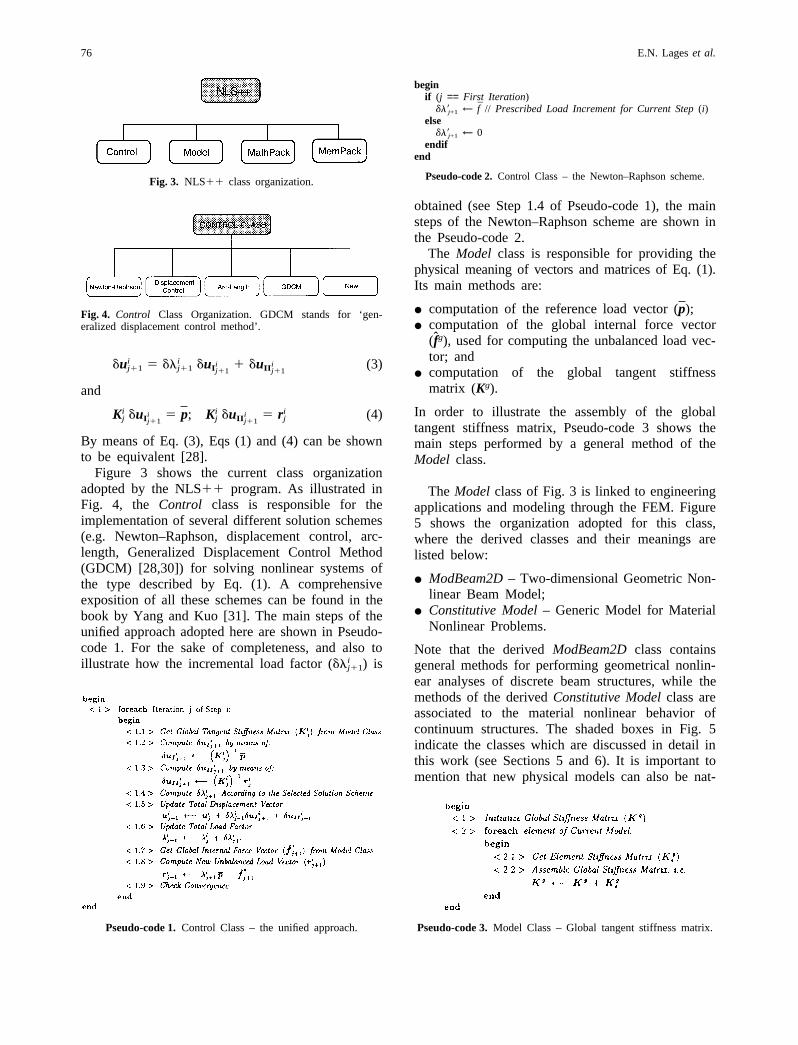
Fig. 3. NLS11 class organization.

Fig. 4. Control Class Organization. GDCM stands for ‘gen-eralized displacement control method’.

duij11 5 dli

j11 duI ij11

1 duII ij11

(3)

and

Kij duI i

j115 p; Ki

j duII ij11

5 r ij (4)

By means of Eq. (3), Eqs (1) and (4) can be shownto be equivalent [28].

Figure 3 shows the current class organizationadopted by the NLS11 program. As illustrated inFig. 4, the Control class is responsible for theimplementation of several different solution schemes(e.g. Newton–Raphson, displacement control, arc-length, Generalized Displacement Control Method(GDCM) [28,30]) for solving nonlinear systems ofthe type described by Eq. (1). A comprehensiveexposition of all these schemes can be found in thebook by Yang and Kuo [31]. The main steps of theunified approach adopted here are shown in Pseudo-code 1. For the sake of completeness, and also toillustrate how the incremental load factor (dli

j11) is

Pseudo-code 1.Control Class – the unified approach.

beginif (j == First Iteration)

dl9j+1 ← f // Prescribed Load Increment for Current Step(i)else

dl9j+1 ← 0endif

end

Pseudo-code 2.Control Class – the Newton–Raphson scheme.

obtained (see Step 1.4 of Pseudo-code 1), the mainsteps of the Newton–Raphson scheme are shown inthe Pseudo-code 2.

The Model class is responsible for providing thephysical meaning of vectors and matrices of Eq. (1).Its main methods are:

I computation of the reference load vector (p);I computation of the global internal force vector

(fg), used for computing the unbalanced load vec-tor; and

I computation of the global tangent stiffnessmatrix (Kg).

In order to illustrate the assembly of the globaltangent stiffness matrix, Pseudo-code 3 shows themain steps performed by a general method of theModel class.

The Model class of Fig. 3 is linked to engineeringapplications and modeling through the FEM. Figure5 shows the organization adopted for this class,where the derived classes and their meanings arelisted below:

I ModBeam2D– Two-dimensional Geometric Non-linear Beam Model;

I Constitutive Model– Generic Model for MaterialNonlinear Problems.

Note that the derivedModBeam2Dclass containsgeneral methods for performing geometrical nonlin-ear analyses of discrete beam structures, while themethods of the derivedConstitutive Modelclass areassociated to the material nonlinear behavior ofcontinuum structures. The shaded boxes in Fig. 5indicate the classes which are discussed in detail inthis work (see Sections 5 and 6). It is important tomention that new physical models can also be nat-

Pseudo-code 3.Model Class – Global tangent stiffness matrix.

77Nonlinear Finite Element Analysis using an Object-Oriented Philosophy

Fig. 5. Model class organization.

urally incorporated in theModel class (see Reference28). Easy incorporation of new models is one ofthe main features of the present FEM OOP system.Finally, MathPack and MemPack (see Fig. 3) areauxiliary classes responsible for general mathemat-ical computations (e.g. norm of a vector, solutionof linear systems of equations) and dynamic memoryallocation, respectively.

5. Geometrically Nonlinear Problems

A brief description of a geometrically nonlinear two-dimensional beam model is given here. It followsthe so-called ‘total formulation’, and is based onthe work by Pacoste and Eriksson [32,33], whichaccounts for shear effects. This model is incorpor-ated in the present FEM OOP system in the parti-cular classModBeam2D(see Fig. 5). The followingderivation gives an idea of the procedures requiredto add a new model in the system.

Figure 6 shows the deformed configuration of aplane beam subjected to large displacements androtations, but small strains. The reference configur-ation corresponds to a straight line element of lengthL, initially on the localx axis.

Each point on the beam axis is subjected to axial(u(x)) and transversal (n(x)) displacements, and isassociated to a generic cross sectionS, which inturn may undergo finite rotations (u(x)), where theabscissax P [0,L] is measured on the reference

Fig. 6. Plane beam: Initial and deformed configurations.

configuration. The deformed configuration isdescribed by means of the position vectorr(x),defined as

r(x) 5 [x 1 u(x)] i 1 v(x) j (5)

where iT 5 [1,0], jT 5 [0,1], and the superscriptT means transpose. Deformation measures can beobtained by writing the tangent vector (­r(x)/­x)with respect to the orthogonal basis (a,b), i.e.

­r(x)­x

5 [1 1 e(x)] a 1 g(x) b (6)

k(x) 5­u(x)

­x

where e(x), g(x) and k(x) are linear strain, angularstrain, and curvature, respectively, and

a(x) 5 cosu(x) i 1 sin u(x) j (7)

b(x) 5 2sinu(x) i 1 cosu(x) j

are unit vectors orthogonal and parallel to thedeformed cross section. In general, the vectors­r(x)/­x anda are not aligned (see Fig. 7). However,alignment is preserved if the angular strain (g(x))is neglected, which occurs, for instance, in beamsdescribed by Bernoulli hypothesis.

Combining Eqs (5), (6) and (7), one obtains

e(x) 5 F 1 1­u(x)

­x G cosu(x)

1­v(x)

­xsinu(x) 2 1

g(x) 5 2 F 1 1­u(x)

­x G sinu(x)

1­v(x)

­xcosu(x) (8)

k(x) 5­u(x)

­x

Fig. 7. Detail of a generic plane beam cross section.

78 E.N. Lageset al.

The internal force (F) and moment (M) acting ona generic cross section can be written as

F 5 N a 1 T b

M 5 M a 3 b (9)

where the symbol3 denotes the cross-product andN, T and M are conjugate scalar variables withrespect to the deformation measures (in the energysense). Note that, according to Fig. 7, the axialforce (N) and the shear force (T) are normal andparallel to the deformed cross section, respectively.Assuming linear constitutive relation, one may write

N 5 EAe

T 5 GAg

M 5 EIk (10)

where EA, GA and EI are the axial, shear andflexural rigidities, respectively. Accordingly, thestrain energyU is given by

U 512EL

0

(EAe2 1 GAg2 1 EIk2) dx (11)

5.1. Finite Element Aspects

The element for performing geometrically nonlinearanalysis of plane frames, taking shear deformationinto account, is described here. It is based on alinear interpolation of the displacement field

uT 5 [u(x), v(x), u(x)]

with respect to the nodal degrees of freedom

(ule)T 5 [ui, vi,ui; uj,vj,uj]

in a local coordinate system, as illustrated by Fig. 8.Equation (11) can be evaluated by one-point

Fig. 8. Finite element for plane beam problems.

Gaussian quadrature. As pointed out by Pacosteand Eriksson [33], the procedure of using reducedintegration avoids locking problems. Once theinterpolation function and the integration strategyare defined, all terms necessary to evaluate Eq. (11)can be computed, e.g.

­u(x)­x

5uj 2 ui

L

­v(x)­x

5vj 2 vi

L

­u(x)­x

5uj 2 ui

L

u(x) 5ui 1 uj

2(12)

The local internal force vector1

S f le DT

5 [Ni,Ti,Mi; Nj,Tj,Mj]

and the local tangent stiffness matrixKle are obtained

by means of the following expressions:

S f le DT

5 F ­U­ui

,­U­vi

, %,­U­uj

G (13)

and

Kle 5

­2U­ui­ui

­2U­ui­vi

%­2U

­ui­uj

Á

­2U­uj­ui

­2U­uj­vi

%­2U

­uj­uj

(14)

respectively. Finally, to obtain the internal forcevector and the tangent stiffness matrix with respectto the global coordinate system (f g

e and Kge,

respectively), a transformation matrixT ; T(w) oforder 6 is defined, wherew is illustrated in Fig. 8.

5.2. Pseudo-codes of ModBeam2D

Pseudo-codes 4–6 illustrate the addition of a nonlin-ear beam model into the computational system.

1 Note that (Ni,Ti,Mi; Nj,Tj,Mj) are the nodal values of the internalforces with respect to the local coordinate system, while (N,T,M)are the internal forces acting on a generic cross-section, accordingto a reference coordinate system as illustrated in Fig. 7.

79Nonlinear Finite Element Analysis using an Object-Oriented Philosophy

Pseudo-code 4.ModBeam2D Class – eneral methods.

Pseudo-code 5.ModBeam2DClass – Element internal force vec-tor.

Pseudo-codes 5 and 6 show how the element internalforce vector (f g

e) and element tangent stiffnessmatrix (Kg

e), respectively, are obtained with respectto the global coordinate system, within the contextof the ModBeam2Dclass. Other models (for per-forming geometrically and/or materially nonlinearanalyses of trusses, for example) can also be easilyadded to the system. This feature (i.e. ‘ease of use’)has been one of the main guiding principles in thedesign of the present FEM OOP environment.

Pseudo-code 6.ModBeam2DClass – Element tangent stiffnessmatrix.

5.3. Example using the ModBeam2D Class

The goal of this section is to illustrate the practicaluse of theModBeam2Dclass by means of a nontriv-ial example of a frame-type structure, which exhibitsa complicated equilibrium path with snap backbehavior. Figure 9 shows a pin-supported planeframe subjected to a single vertical concentratedload. This problem was originally presented by Leeet al. [34], and was also later studied by severalresearchers such as Frey and Cescotto [35], Schwei-zerhof and Wriggers [36], Simo and Vu-Quoc [37],Chen and Blandford [38] and Pacoste and Eriksson[33]. Lee et al. [34] have presented an analyticalsolution for the structural behavior of their frameproblem, which is characterized by large displace-ments and rotations. However, they did not considershear effects in their derivations. These effects areconsidered in the formulation implemented in theModBeam2Dclass.

Fig. 9. Lee frame example description.

80 E.N. Lageset al.

The numerical data adopted for the Lee frameexample is also presented in Fig. 9. Because a loadcontrol algorithm (e.g. Newton–Raphson) cannotcapture snap back behavior, this problem was solvedby means of the GDCM [30,39] (see Fig. 4). Theincremental-iterative solution procedure was carriedout with 200 steps, and the maximum number ofiterations that occurred in a step was 3. The conver-gence criterion was established in terms of the ratioof the Euclidean norms of the unbalanced forces(residual) and the reference load vector. Since thelatter is the unit for this example, the tolerance(TOL) is the norm of the unbalanced forces whichwas set as TOL5 0.001. The CPU time in a SUNSunSPARCstation 20 (96 Mbytes of memory) was46 seconds.

The load-displacement curves corresponding tothe displacementsu and v, at the load applicationpoint (fixed-point load), are given in Fig. 10, whereeach dot on the curves corresponds to one step.These results clearly show snap back behavior. Thecapital letters in Fig. 10 denote a point in thesolution path corresponding to the deformed shapes(for various load levels) shown in Fig. 11. Theresults obtained here are in agreement with thoseobtained by the program MASTRAN2 (MatrixStructural Analysis 2) [40]. For instance, the limitload obtained in the present study is 18.792KN (seeFig. 10), and the MASTRAN2 result consideringclassical beam theory (i.e. no transverse sheareffect2) is 18.454KN.

6. Materially Nonlinear Problems

Many materials (e.g. metals, polymers, ceramics,soil, concrete and rock) may fail by some form oflocalization of deformation. Consider, for example,the compression test illustrated in Fig. 12. Localiz-ation is often followed by a decrease of the loadbearing capacity after reaching the peak load. Itoften leads to fracture (either ductile or brittle)because the deformations accumulated in the smalllocalization band facilitate rupture. As illustrated byFig. 12, an initially homogeneous state of defor-mation is differentiated from the one at the localiz-ation band, where the deformation incrementslocalize in a small region of the material. Experi-mental findings indicate that there is a relationshipbetween the size of the localization band and the

2 At the time of this writing, MASTRAN2 uses the simplifiednotion of shear area (As) to deal with transverse shear defor-mation, however, this consideration was not employed here.

Fig. 10. Load 3 displacement curves.

Fig. 11. Deformed shapes.

material microstructure. Thus, the important notionof a ‘characteristic length’, which sets the size ofthe band, is introduced.

With respect to the behavior described above,consider the constitutive (stress/strain) relation

81Nonlinear Finite Element Analysis using an Object-Oriented Philosophy

Fig. 12. Macroscopic behavior in a compression test.

through an homogenization procedure with respectto the results of the test. The applied force is dividedby the cross-sectional area and the displacement atthe tip of the bar is divided by a certain gage length(e.g. the initial length of the bar). Therefore, theobserved macroscopic (stress/strain) behavior isdescribed in a pointwise fashion.

After discretization of the continuum by the FEM,the numerical solutions show pronounced depen-dence upon the discretization level, and are thereforephysically inconsistent [41]. The reason for this isbecause classical constitutive models are expressedin terms of (averaged) stresses and strains definedlocally. When a localized deformation mode getsactivated by a local defect, the characteristic defor-mation scale and the microstructure size becomecomparable. The state of the material at a pointdepends on the deformation history of a certainneighborhood of this point (i.e. the material behavioris nonlocal). Therefore, to remedy the situation, aninternal length scale (characteristic length) is usedin the continuum description.

Enhanced continuum models provide a consistenttreatment of localization problems, e.g. Cosserat(micropolar) continuum, nonlocal (integral) model,and higher-order gradient continuum. Here, an elas-toplastic model within the framework of Cosserat

s11

s22

s33

s12

s21

m13

m23

5

2G(1−n)

1−2n

2Gn

1−2n

2Gn

1−2n0 0 0 0

2Gn

1−2n

2G(1−n)1−2n

2Gn

1−2n0 0 0 0

2Gn

1−2n

2Gn

1−2n

2G(1 − n)1−2n

0 0 0 0

0 0 0 G 1 a G − a 0 0

0 0 0 G − a G 1 a 0 0

0 0 0 0 0 2G,2 0

0 0 0 0 0 0 2G,2

g11

g22

g33

g12

g21

k13

k23

(17)

continuum, and its corresponding implementationusing object-oriented concepts, are presented [42].Additional strain (curvatures) and stress (couple-stress) measures enter the kinematic and staticdescription of the continuum, which require theintroduction of additional material parameters(internal length scale). In this way, the boundaryvalue problem remains well-posed after strain local-ization occurs [43].

6.1. Cosserat (Micropolar) Continuum

In the Cosserat continuum (also denoted micropolarcontinuum), the microstructure of the material isexplicitly taken into account, which permits to dif-ferentiate the rotation of the continuum(macrorotation) from the rotation of the microstruc-ture (microrotation) [44,45]. This leads to the follow-ing (linear) strain tensors

gij 5 uj,i 2 eijkfk (15)

kij 5 fj,i (16)

where ui and fi are the displacement and microro-tation vectors, respectively, andeijk is the alternatortensor. The tensorgij is associated to change ofdimensions and distortion, while the tensorkij isassociated to curvatures and twist of microstructure.Figure 13 shows the generalized stresses associatedwith the strain measures. The stress tensor is nowcomposed of stressessij and couple-stressesmij , andit is not necessarily symmetric anymore.

For plane strain and no initial stresses or defor-mations, the constitutive relationship for the linearelastic and isotropic material is given by Eq. (17),whereG and n are classical parameters, denoted asshear modulus and Poisson ratio, respectively. Theparametera relates the stiffness between the macror-otation and the microrotation, and the parameter,

82 E.N. Lageset al.

Fig. 13. Stress components for micropolar continuum.

has the dimension of length, and therefore introducesa length scale in the continuum description.

The differential equations of equilibrium areexpressed by

sji ,j 1 fi 5 0 (18)

mji ,j 1 eijk sjk 1 Ii 5 0 (19)

where fi and Ii are body forces and body couplesper unit volume, respectively.

In this enriched continuum, the boundary con-ditions to be specified are

sji nj 5 ti in St or ui 5 ui in Su (20)

mji nj 5 mi in Sm or fi 5 fi in Sf (21)

where St, Sm, Su and Sf denote regions of theboundary with prescribed stress, couple-stress, dis-placements and microrotations, respectively.

6.2. Cosserat Elastoplastic Model

The main feature of Cosserat elastoplasticity is theuse of the classical plasticity framework [46] byaugmenting the vectors and matrices involved. Thisleads to an elegant formulation, which is also naturalto the OOP philosophy.

The yield function adopted here is a generalizationof the classical von Mises criterion, and it isgiven by

f 5 Î3J2 2 s(b) (22)

where J2 is the second invariant of the deviatoricstresses, ands(b) is the yield stress which dependsupon the hardening (or softening) parameterb. Thespecific function adopted in this work is

s(b) 5 sY 1 hb (23)

where sY is the yield stress, andh is the plasticmodulus. Other hardening functions can also beemployed within the present framework of analysis.

As usually done in computational solid mechanics,the strain and stress tensors are recast in vectorform. All the strain components are assembled inthe strain vector

gT 5 [g11 g22 g33 g12 g21 u k13, k23, ] (24)

where the length parameter, has been introducedso that all entries ing are dimensionless. Accord-ingly, the stress components are assembled in thestress vector

sT 5 [s11 s22 s33 s12 s21 u m13/, m23/,] (25)

In compact notation,J2 (see Eq. (22)) can berewritten as [47,48]

J2 512

si Pij sj (26)

where

P =

23

213

213

0 0 0 0

213

23

213

0 0 0 0

213

213

23

0 0 0 0

0 0 012

12

0 0

0 0 012

12

0 0

0 0 0 0 0 1 0

0 0 0 0 0 0 1

(27)

According to the plasticity criterion adopted here,the material is not sensitive to the hydrostatic andanti-symmetric states of the stress tensor. For apoint (sij , b) on the yield surface, the flow rule(associated) is given by

g·pi 5

3l·

2s(b)Pij sj (28)

where the superscriptp stands for plastic, and thesuperimposed dot refers to the rate variation, whichis a standard terminology in theoretical and compu-tational inelasticity. The variation of the parameterb, which is conjugate to the definition ofJ2 [46], is

b·

5 !23

g·pi Pij g·p

j (29)

leading to

b·

5 l· (30)

83Nonlinear Finite Element Analysis using an Object-Oriented Philosophy

6.3. Class Organization

In general, the establishment of equilibrium in asystem exhibiting material nonlinear behavior canbe understood in two levels: first, theglobal equilib-rium, which is considered here through the environ-ment NLS11 (see Section 4) and, secondly, thelocal equilibrium, at the level of quadrature pointswith specific treatment for each constitutive model.The discretization procedure used in thestructuralmodel class, which is part of the NLS11 environ-ment, is responsible for defining the internal forcevector of the structure, as well as its tangent stiffnessmatrix. In the FEM context, these quantities aregenerated from contributions of the elements in themesh, which are evaluated by means of pieces ofinformation obtained in a finite number of points(i.e. quadrature points). To build the internal forcevector, the basic problem consists of determiningthe increment of stress at the integration point, fromthe increment of deformation. The tangent stiffnessmatrix is defined such that it is consistent with thecurrent deformation state [46].

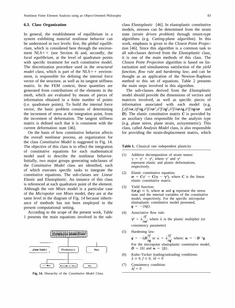
On the basis of how constitutive behavior affectsthe overall nonlinear process, an organization forthe classConstitutive Modelis suggested in Fig. 14.The objective of this class is to effect the integrationof constitutive equations for each mathematicalmodel used to describe the nonlinear behavior.Initially, two major groups generating subclasses ofthe Constitutive Modelclass are identified, eachof which executes specific tasks to integrate theconstitutive equations. The sub-classes are:LinearElastic and Elastoplastic. An instance of this classis referenced at each quadrature point of the element.Although thevon Misesmodel is a particular caseof the Micropolar von Misesmodel, they are at thesame level in the diagram of Fig. 14 because inherit-ance of methods has not been employed in thepresent computational setting.

According to the scope of the present work, Table1 presents the main equations involved in the sub-

Fig. 14. Hierarchy of theConstitutive Model Class.

classElastoplastic [46]. In elastoplastic constitutivemodels, stresses can be determined from the strainstate (strain driven problem) through return-typealgorithms (e.g.Cutting-plane algorithm). In thiswork, emphasis is given to theClosest Point Projec-tion [46]. Since this algorithm is a common task toall sub-classes derived from theElastoplasticclass,it is one of the main methods of this class. TheClosest Point Projectionalgorithm is based on lin-earization and simultaneous satisfaction of theyieldfunction, flow ruleand hardening law; and can bethought as an application of the Newton–Raphsonmethod to this set of equations. Table 2 presentsthe main steps involved in this algorithm.

The sub-classes derived from theElastoplasticmodel should provide the dimensions of vectors andmatrices involved, as well as specific pieces ofinformation associated with each model (e.g.f,­f/­s,­f/­q,­2f/­s2,­2f/­q2,­2f/­s­q,­2f/­q­s andD). The elastic constitutive matrixC is provided byan auxiliary class responsible for the analysis type(e.g. plane stress, plane strain, axisymmetric). Thisclass, calledAnalysis Modelclass, is also responsiblefor providing the strain-displacement matrix, which

Table 1. Classical rate independent plasticity

(1) Additive decomposition of strain tensor:g 5 ge 1 gp, wherege and gp

represent elastic and plastic deformations,respectively.

(2) Elastic constitutive equation:s 5 Cge 5 C(g 2 gp), whereC is the linearelastic constitutive matrix.

(3) Yield function:f(s,q) # 0, wheres and q represent the stressstate and the internal variables of the constitutivemodel, respectively. For the specific micropolarelastoplastic constitutive model presented,q 5 2{ hb}.

(4) Associative flow rule:

g·p 5 l

· ­f­s

, where l· is the plastic multiplier (or

consistency parameter)

(5) Hardening law:

q· 5 2l·D

­f­q

or a·

5 l· ­f­q

, where:a 5 2D21q.

For the micropolar elastoplastic constitutive model,D 5 [h] and a 5 { b}.

(6) Kuhn–Tucker loading/unloading conditions:l·

$ 0, f # 0, l·f 5 0

(7) Consistency condition:l·f· 5 0

84 E.N. Lageset al.

Table 2. Closest point projection algorithm

(1) Initialize:k 5 0, gp(k)

n11 5 gpn, a(k)

n11 5 an, Dl(k)n11 5 0

(2) Compute stresses, internal variables, yield functionand flow rule/hardening law residuals:

s(k)n11 5 C S gn11 2 gp(k)

n11 Dq(k)

n11 5 2D a(k)n11

f(k)n11 5 f Ss(k)

n11,q(k)n11 D

R(k)n11 5 H 2gp(k)

n11 1 gpn11

2a(k)n11 1 an

J 1 Dl(k)n11 5

­f(k)n11

­s

­f(k)n11

­q6

(3) If f(k)n11 # TOL1 and iR (k)

n11i # TOL2 then STOP,else:

(4) Compute Hessian matrix of the Newton’s problem:

S A(k)n11 D21

5

3 C21 1 Dl(k)n11

­2f(k)n11

­s2 Dl(k)n11

­2f(k)n11

­s­q

Dl(k)n11

­2f(k)n11

­q­sD21 1 Dl(k)

n11

­2f(k)n11

­q2

4(5) Compute increment of increment of plastic

consistency parameter:

DDl(k)n11 5

f(k)n11 2 F S ­f(k)

n11

­s DT S ­f(k)n11

­q DT G A(k)n11R(k)

n11

F S ­f(k)n11

­s DT S ­f(k)n11

­q DT G A(k)n11 5

­f(k)n11

­s

­f(k)n11

­q6

(6) Obtain incremental plastic strains and internalvariables:

H Dgp(k)

n11

Da(k)n11

J 5 F C21 0

0 D21 G A(k)n11

5 R(k)n11 1 DDl(k)

n11 5­f(k)

n11

­s

­f(k)n11

­q66

(7) Update state variables and increment ofconsistency parameter:gp(k11)

n11 5 gp(k)

n11 1 Dgp(k)

n11

a(k11)n11 5 a(k)

n11 1 Da(k)n11

Dl(k11)n11 5 Dl(k)

n11 1 DDl(k)n11

(8) k 5 k 1 1 and GOTO Step (2).

is used for computing the element internal forcevector and the element tangent stiffness matrix. Thisis an auxiliary class for theConstitutive Modelclass, which plays a role somehow analogous to theauxiliary classesMathPack and MemPack of theNLS11 system, illustrated in Fig. 3. Improvementin computational performance can be achieved ifthe inverses ofC and D are also provided by thecorresponding classes.

When the structure reachesglobal equilibrium,the Elastoplasticclass requires a method for updat-ing the ‘state variables’ at the equilibrium point(e.g.gp

n11 andan11). Finally, the tangent constitutivematrix must be defined in theElastoplastic class.Here the so-calledAlgorithmic Tangent ElastoplasticModuli is used, which is consistent with the algor-ithm employed to update the stresses [46], and itleads to

Cepalg 5 An11 2 (31)

C if l· 5 0

An11

­fn11

­s S­fn11

­s DT

An11

F S ­fn11

­s DT S ­fn11

­q DT GAn11

­fn11

­s

­fn11

­q

if l· . 0

where An11 is given in Step 4 of Table 2. It isworth noting that for a linear elastic analysis, thematrix C is not modified by theLinear Elasticclass, and for an elastoplastic analysis, it is modifiedaccording to Eq. (31). Thus, whenever necessary,the derived classes of theConstitutive Modelclasscan modify the matrixC.

6.4. Example Involving Localization ofDeformation

To demonstrate that the present implementationworks and to illustrate the use of the OOP environ-ment, consider the compression test illustrated inFig. 15, in which strain localization into a shearband takes place at the onset of softening. Thisfigure illustrates the geometry and boundary con-ditions of the test specimen, which is modeled as aplane strain problem. The bottom edge does notmove and the upper edge is constrained to move asa linear segment (without rotation). For comparison,this problem is analyzed using both classical andCosserat elastoplastic models.

The problem domain is discretized with 9-node

85Nonlinear Finite Element Analysis using an Object-Oriented Philosophy

Fig. 15. Compression test layout.

Table 3. Numerical results for the classical continuuma

Discretization #DOF #Steps #Iterations(max)

08316 1056 240 1116332 4160 136 1428356 12656 92 76

aSUN SunSPARCstation 20 with 96 Mbytes of memory runningSunOS 4.1.4

quadratic Lagrangian finite elements using Gaussianintegration with nine quadrature points per element.The nonlinear system of equations is solved bymeans of the GDCM (see Fig. 4), which is thesame method employed to solve the Lee frame inSection 5.3. The tolerance criterion for convergenceof the iterations is defined as the ratio between thenorm of the unbalanced force vector and the normof the reference force vector, and it is set as TOL5 0.0001. To follow an equilibrium path associatedwith a localized deformation mode, a relatively small(1% of the vertical loading) uniformly distributedhorizontal loading at the upper face, and a 5%reduction ofsY for the element with bottom right-hand side node located at L/8 from the bottom edgeof the specimen (see Fig. 15) are used.

6.4.1. FEA Using Classical Elastoplastic ModelThe values of the parameters necessary to performthis analysis are given in Fig. 15. Three levels ofmesh discretization are employed, and the deformedconfigurations for the final step of the analyses areshown in Figs 16, 17 and 18. For each discretization,Table 3 shows the number of degrees of freedom(#DOF) in the finite element model, the total number

of steps (#Steps), and the maximum number ofiterations in a step (#Iterations (max)).

Figure 19 shows the relation between the appliedload level and the vertical displacement at the upperface of the test specimen for different discretizationlevels. This graph shows that the descendingbranches of the curve tend to get closer to theascending branch as the mesh is refined. The resultsalso depend on the arrangement of the elements, i.e.exhibit directional bias. Moreover, the deformationtend to localize in a region of zero thickness (seeFigs 16, 17 and 18) with vanishing dissipativeenergy. This pathological behavior is remedied bymeans of the micromorphic continuum model, whichis discussed next.

6.4.2. FEA Using Cosserat Elastoplastic ModelIn this analysis, the degrees of freedom correspond-ing to microrotation are set free for all the nodes ofthe finite element meshes. The additional parametersrequired for the Cosserat material are also given inFig. 15. The same initial meshes adopted in theclassical analysis are used here, and the deformedconfigurations for the final step of the analyses areshown in Figs 20, 21 and 22. Selected representativeresults are provided in Table 4, which uses the samenomenclature as Table 3.

The equilibrium trajectories for the various levelsof discretization are given in Fig. 23, which showsreduced sensitivity to mesh refinement, leading to amore stable solution. The agreement on the post-peak trajectory, especially for the meshes 163 32and 283 56, guarantees a finite dissipative energyand localization to a band of finite thickness (seeFigs 20, 21 and 22).

6.4.3. ComparisonIt is worth comparing Table 3, and Figs 16, 17, 18and 19 for the classical elastoplastic model withTable 4, and Figs 20, 21, 22 and 23 for the Cosseratelastoplastic model. In Figs 16 to 18, and 20 to 22,the deformations have been amplified by a factor of15. Moreover, the CPU time required by theCosserat continuum is approximately three times theone required by the classical continuum.

7. Conclusions and Extensions

An OOP framework for solving physical problemsin solid and structural mechanics, by means of theFEM, has been presented. The approach adoptedherein consists of using OOP as atool, which playsa crucial role in the application of the FEM to the

86 E.N. Lageset al.

Fig. 16. Classical: 83 16. Fig. 17. Classical: 163 32. Fig. 18. Classical: 283 56.

Fig. 19. Equilibrium trajectories for the classical continuum. Theinclination of the post-peak branch is different for each mesh.

solution of engineering mechanics problems. Specificapplications involve a geometrically nonlinear beammodel and the elastoplastic Cosserat continuum.Examples have been provided, which illustrate themain features of the computational system.

The overall class organization for nonlinear mech-anics modeling has been presented. All analyses rely

Table 4. Numerical results for the Cosserat continuuma

Discretization #DOF #Steps #Iterations(max)

08316 1617 320 2616332 6305 224 2228356 19097 184 20

aSUN SunSPARCstation 20 with 96 Mbytes of memory runningSunOS 4.1.4

on a general control class where several classical(e.g. Newton–Raphson) and modern (e.g. arc-length)nonlinear solution schemes are available.

Potential extensions of this work include develop-ment of a parallel computing object orientedenvironment, and extension of the present ideas toother numerical methods, such as the BoundaryElement Method (BEM). It would be interesting tointegrate the parallel computing techniques presentedby Hsieh et al. [49,50] with the present ideas onfinite element analysis using OOP, and additionalconcepts on distributed data objects and tasks. Withrespect to extension of the OOP framework to othernumerical methods, it is worth investigating appli-cations of OOP to novel numerical techniques suchas the symmetric-Galerkin BEM [51, 52]. Thesetopics are currently under investigation by theauthors.

87Nonlinear Finite Element Analysis using an Object-Oriented Philosophy

Fig. 20. Micropolar: 8 3 16. Fig. 21. Micropolar: 16 3 32. Fig. 22. Micropolar: 28 3 56.

Fig. 23. Equilibrium trajectories for the Cosserat continuum. Theinclination of the post-peak branch shows reduced sensitivity tomesh refinement, especially for the finer meshes.

Acknowledgements

GHP thanks the United States National Science Foundation(NSF) through grant No. CMS-9713798 (Mechanics andMaterials Program). IFMM acknowledges the financialsupport provided by FAPERJ (Fundac¸ao de Amparo a`Pesquisa do Estado do Rio de Janeiro), and RRS acknowl-edges CNPq (Conselho Nacional de Desenvolvimento

Cientifico e Tecnolo´gico), which are Brazilian agenciesfor research and development. Finally, all the authorswould like to thank two anonymous reviewers for valuablesuggestions which contributed to substantial improvementsto this paper.

References

1. Roux, S. (1966) Continuum and discrete descriptionof elasticity and other rheological behavior. In: Herm-ann, H.J.; Roux, S. (eds), Statistical Models for theFracture of Disordered Media, North-Holland, pp 87–114

2. Dahl, O.J.; Nygaard, K. (1966) SIMULA – An Algol-based simulation language. Communications of theACM 9, 671–678

3. Fenves, G.L. (1990) Object-oriented programming forengineering software development. Engineering withComputers 6, 1–15

4. Goldberg, A.; Robson, D. (1983) Smalltalk-80: TheLanguage and its Implementation. Addison-Wesley,Reading, MA

5. Stefik, M.; Bobrow, D.G. (1985) Object oriented pro-gramming: themes and variations. AI Magazine 40–62

6. Weinreb, D.; Moon, D. (1981) Lisp machine manual.Symbolics Inc.

7. Cox, B.J. (1986) Object Oriented Programming.Addison-Wesley, Reading, MA

8. Stroustrup, B. (1997) The C11 Programming Langu-age, third edition. Addison-Wesley, Reading, MA

9. Zimmermman, Th.; Dubois-Pe`lerin, Y.; Bomme, P.(1992) Object-oriented finite element programming: I.Governing principles. Computer Methods in AppliedMechanics and Engineering 98, 291–303

10. Rehak, D.R.; Baugh Jr., J.W. (1989) Alternative pro-

88 E.N. Lageset al.

gramming techniques for finite element program devel-opment. IABSE Colloquium on Expert Systems inCivil Engineering, Bergamo, Italy

11. Forde, B.W.R; Foschi, R.O.; Stiemer, S.F. (1990)Object-oriented finite element analysis: Computers andStructures 34(3), 355–374

12. Dubois-Pe`lerin, Y.; Zimmermman, Th.; Bomme, P.(1992) Object-oriented finite element programming: II.A prototype program in smalltalk. Computer Methodsin Applied Mechanics and Engineering 98, 361–397

13. Dubois-Pe`lerin, Y.; Zimmermman, Th. (1993) Object-oriented finite element programming: III. An efficientimplementation in C11. Computer Methods inApplied Mechanics and Engineering 108, 165–183

14. Zimmermman, Th.; Eyheramendy, D. (1996) Object-oriented finite elements I. Principles of symbolic deri-vations and automatic programming. ComputerMethods in Applied Mechanics and Engineering132(3–4), 259–276

15. Eyheramendy, D.; Zimmermman, Th. (1996) Object-oriented finite elements II. A symbolic environmentfor automatic programming. Computer Methods inApplied Mechanics and Engineering 132(3–4), 277–304

16. Eyheramendy, D.; Zimmermman, Th. (1998) Object-oriented finite elements III. Theory and application ofautomatic programming. Computer Methods inApplied Mechanics and Engineering 154 (1–2), 41–68

17. Menetrey, P.; Zimmermann, Th. (1993) Object-ori-ented nonlinear finite element analysis: application toJ2 plasticity. Computers and Structures 49(5), 767–777

18. Mackie, R.I. (1992) Object oriented programming ofthe finite element method. International Journal forNumerical Methods in Engineering 35, 425–436

19. Alves Filho, J.S.R; Devloo, P.R.B. (1991) Object ori-ented programming in scientific computations: Thebeginning of a new era. Engineering Computations 8,81–87

20. Raphael, B.; Krishnamoorthy, S. (1993) Automaticfinite element development using object oriented tech-niques. Engineering Computations 10(3), 267–278

21. Bettig, B.P.; Han, R.P.S. (1996) An object-orientedframework for interactive numerical analysis in agraphical user interface environment. InternationalJournal for Numerical Methods in Engineering 39(17),2945–2971

22. Besson, J.; Foerch, R. (1997) Large scale object-oriented finite element code design. ComputerMethods in Applied Mechanics and Engineering 142(1–2), 165–187

23. Jeremic´, B.; Sture, S. (1998) Tensor objects in finiteelement programming. International Journal forNumerical Methods in Engineering 41(1), 113–126

24. Noronha, M.; Wagner, M.; Wirnitzer, J.; Dumont,N.A.; Gaul, L. (1996) On a robust object-orientedcode for the implementation of conventional andhybrid boundary element methods. In SIBRAT(Simposio Brasileiro sobre Tubulac¸oes e Vasos dePressa˜o), Rio de Janeiro, Brazil, pp 239–241

25. Lage, C. (1998) The application of object-orientedmethods to boundary elements. Computer Methodsin Applied Mechanics and Engineering 157 (3–4),205–213

26. Olsson, A. (1998) An object-oriented implementation

of structural path following. Computer Methods inApplied Mechanics and Engineering 161 (1–2), 19–47

27. Lafore, R. (1991) Objected-Oriented Programming inTURBO C11. Waite Group Press, A Division of theWaite Group, Inc, first edition

28. Paulino, G.H.; Menezes, I.F.M; Lages, E.N. A unifiedapproach for solving nonlinear finite element sys-tems—Implementation and Applications (to besubmitted)

29. Batoz, J.L.; Dhatt, G. (1979) Incremental displacementalgorithms for nonlinear problems. International Jour-nal for Numerical Methods in Engineering 14,1262–1267

30. Yang, Y.B.; Shieh, M.S. (1990) Solution method fornonlinear problems with multiple critical points. AIAAJournal 28 (12), 2110–2116

31. Yang, Y.B.; Kuo, S.R. (1994) Theory & Analysis ofNonlinear Framed Structures. Prentice-Hall, New York

32. Pacoste, C.; Eriksson, A. (1995) Element behaviourin post-critical plane frame analysis. ComputerMethods in Applied Mechanics and Engineering 125(1–4), 319–343

33. Pacoste, C.; Eriksson, A. (1997) Beam elements ininstability problems. Computer Methods in AppliedMechanics and Engineering 144 (1–2), 163–197

34. Lee, S-L.; Manuel, F.S.; Rossow, E.C. (1968) Largedeflections and stability of elastic frames. Journal ofEngineering Mechanics (ASCE) 94(EM2), 521–547

35. Frey, F.; Cescotto, S. (1977) Some new aspects of theincremental total Lagrangian description in nonlinearanalysis. International Conference on Finite Elementsin Nonlinear Solid and Structural Mechanics, vol 1,Geilo, Norway, pp 323–343

36. Schweizerhof, K.H.; Wriggers, P. (1986) Consistentlinearization for path following methods in nonlinearfinite element analysis. Computer Methods in AppliedMechanics and Engineering 59, 261–279

37. Simo, J.C.; Vu-Quoc, L. (1986) A three-dimensionalfinite-strain rod model. Part II: computational aspects.Computer Methods in Applied Mechanics and Engin-eering 58, 79–116

38. Chen, H.; Blandford, G.E. (1993) Work-increment-control method for nonlinear analysis. InternationalJournal for Numerical Methods in Engineering 36,909–930

39. Menezes, I.F.M.; Lages, E.N.; Paulino, G.H. (1997)A unified approach for solving nonlinear finite elementsystems of equations. In M.S. Shephard (ed) FourthU.S. National Congress on Computational Mechanics,San Francisco, CA, p 138

40. McGuire, W.; Gallagher, R.H.; Ziemian, R.D. (1999)Matrix Structural Analysis. John Wiley, New York,second edition

41. Bazant, Z.P. (1986) Mechanics of distributed cracking.Applied Mechanics Reviews 39(5), 675–705

42. Lages, E.N. (1997) Modeling of strain localizationwith generalized continuum theories. PhD thesis,Department of Civil Engineering, PUC-Rio, Rio deJaneiro, Brazil, (in Portuguese)

43. de Borst, R.; Sluys, L.J.; Mu¨hlhaus, H-B.; Pamin, J.(1993) Fundamental issues in finite element analysesof localization of deformation. Engineering Compu-tations 10(2), 99–121

44. Iordache, M-M.; Willam, K. (1998) Localized failure

89Nonlinear Finite Element Analysis using an Object-Oriented Philosophy

analysis in elastoplastic Cosserat continua. ComputerMethods in Applied Mechanics and Engineering 151,559–586

45. Mori, K.; Shiomi, M.; Osakada, K. (1998) Inclusionof microscopic rotation of powder particles duringcompaction in finite element method using Cosseratcontinuum theory. International Journal for NumericalMethods in Engineering 42(5), 847–856

46. Simo, J.C.; Hughes, T.J.R. (1988) Elastoplasticity andViscoplasticity – Computational Aspects. StanfordUniversity, Department of Applied Mechanics

47. de Borst, R. (1991) Simulation of strain localization:A reappraisal of the Cosserat continuum. EngineeringComputations 8, 317–332

48. de Borst, R. (1993) A generalisation of J2-flow theoryfor polar continua. International Journal for NumericalMethods in Engineering 103(3), 347–362

49. Hsieh, S-H.; Paulino, G.H.; Abel, J.F. (1995) Recur-

sive spectral algorithms for automatic domain par-titioning in parallel finite element analysis. ComputerMethods in Applied Mechanics and Engineering 121(1–4), 137–162

50. Hsieh, S.-H.; Paulino, G.H.; Abel, J.F. (1997) Evalu-ation of automatic domain partitioning algorithms forparallel finite element analysis. International Journalfor Numerical Methods in Engineering 40(6), 1025–1051

51. Gray, L.J.; Paulino, G.H. (1997) Symmetric Galerkinboundary integral formulation for interface and multi-zone problems. International Journal for NumericalMethods in Engineering 40 (16), 3085–3101

52. Paulino, G.H.; Gray, L.J. Error estimation and adaptiv-ity for the symmetric Galerkin boundary elementmethod. Journal of Engineering Mechanics (ASCE)(in press)