Nonlinear dynamics and statistical physics of DNA.

Michel PeyrardLaboratoire de Physique, Ecole Normale Superieure de Lyon,

46 allee d’Italie, 69364 Lyon Cedex 07, France.(Dated: January 16, 2004)

DNA is not only an essential object of study for biologists. it raises very interesting questionsfor physicists. This paper discuss its nonlinear dynamics, its statistical mechanics, and one ofthe experiments that one can now perform at the level of a single molecule and which leads to anon-equilibrium transition at the molecular scale.

After a review of experimental facts about DNA, we introduce simple models of the molecule andshow how they lead to nonlinear localization phenomena that could describe some of the experimen-tal observations. In a second step we analyze the thermal denaturation of DNA, i.e. the separationof the two strands using standard statistical physics tools as well as an analysis based on the prop-erties of a single nonlinear excitation of the model. The last part discusses the mechanical openingof the DNA double helix, performed in single molecule experiments. We show how transition statetheory combined with the knowledge of the equilibrium statistical physics of the system can be usedto analyze the results.

I. INTRODUCTION

The famous book of E. Schrodinger “What is life?” [1] was one of the first attempts to use the laws of physicsand chemistry to analyze the basic phenomena of life, and in particular the properties of DNA, the molecule thatencodes the information that organisms need to live and reproduce themselves. Fifty years after the discovery of itsdouble helix structure [2] DNA is still fascinating physicists, as well as the biologists, who try to unveil its remarkableproperties.It is now well established that the static structure of biological molecules is not sufficient to explain their function.This is particularly true for DNA which undergoes large conformational changes during transcription (i.e. the readingof the genetic code) or replication. This is why it is important to study the dynamics of the molecule. Owing tothe large amplitude motions which are involved, its nonlinear aspect cannot be ignored, and this is what makes itparticularly interesting. However pure dynamical studies are not sufficient because the thermal fluctuations play amajor role in DNA functioning. Therefore they must be completed by statistical mechanics investigations to yielduseful results.This paper, which emerged from a series of graduate lectures given in the university of Madrid does not attemptto present a complete review of the numerous studies devoted to nonlinear dynamics of DNA, which is available inthe book Nonlinear physics of DNA [3]. Instead it focuses on a few nonlinear dynamical models for which non onlynonlinear dynamics but also statistical mechanics has been investigated, and it tries to motivate the models and theirparameters in order to allow the reader to build his/her own model and analysis.

II. DNA: STRUCTURE, FUNCTION AND DYNAMICS

A. DNA in biology

There are two major classes of biological molecules, proteins and nucleic acids. Proteins perform most of the functionsin a living organism. They are active machines that catalyze some chemical reactions, transport other molecules suchas oxygen (transported by hemoglobin), make controllable ion channels across membranes, self assemble to formsome rigid structures in a cell such as the cytoskeleton, act as molecular motors responsible for instance of musclecontraction, and many other tasks.The “map” to build these proteins is given by the genetic code stored within the structure of DNA, the DeoxyriboseNucleic Acid. DNA makes up the genome of an organism and for instance the human genome is made of 46 pieces,present in each cell, the chromosomes. Ingenious experiments have shown that each chromosome is made of a singleDNA molecule which is 4 to 10 cm long [4, 5]! Therefore the genome stored in each of our cells has a length of about2 m. And humans do not have the privilege of the longest genome: the salamander has a genome of about 1 km. Ofcourse this very long genome has to be highly compacted to fit into a cell, into a very elaborate hierarchical structurewhich is the subject of intense studies.

2

1. The structure of DNA.

DNA is a polymer, or, more precisely a set of two entangled polymers. Its structure is presented in details in thebooks of Saenger [6] and Calladine [7] and shown on fig. 1. Each of the monomers that make up these polymers is a

FIG. 1: The double helix structure of DNA shown in a full atomic representation (left) and schematically (right).

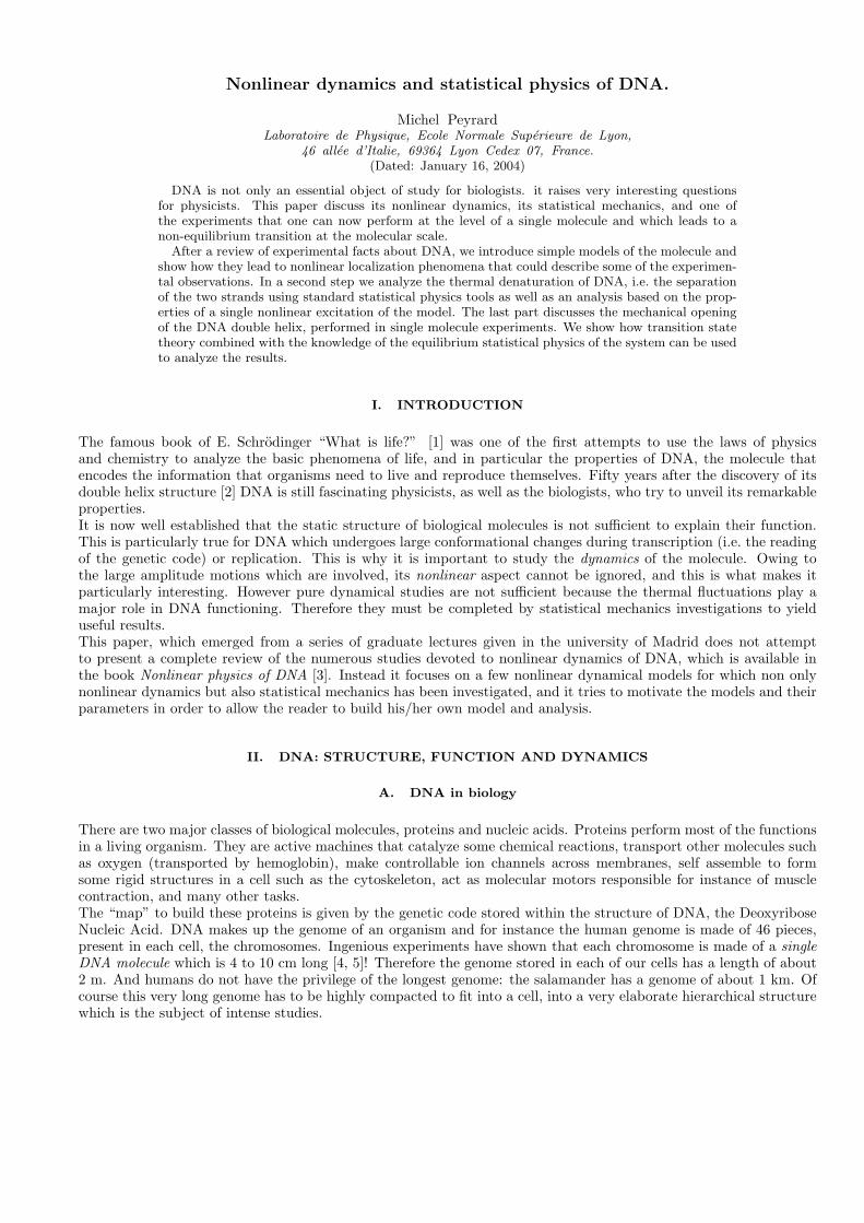
nucleotide which a compound of three elements: a phosphate group PO−4 , a sugar ring, i.e. a five-atom cyclic group,

and a base which is a complex organic group that can have one or two cycles. Figure 2 shows a schematic view ofthe chain of nucleotides. The backbone is formed by a sequence of phosphate groups and sugars, and it is orientedbecause on one side of the sugar the phosphate group is linked to a carbon atom that does not belong to the sugarring while, on the other side, it is linked to a carbon atom which is part of the sugar ring.

PO

O

O

O

CH 2

CH

CH

CH2

CH

O

O

CH

NNC

CCH NH2

O

P

PS S PP

B’BPhosphate

Sugar

next Phosphate

Base(cytosine)

(a) (b)

FIG. 2: (a) An example of a nucleotide of DNA. (b) Schematic view of the chain of nucleotides along one DNA strand.

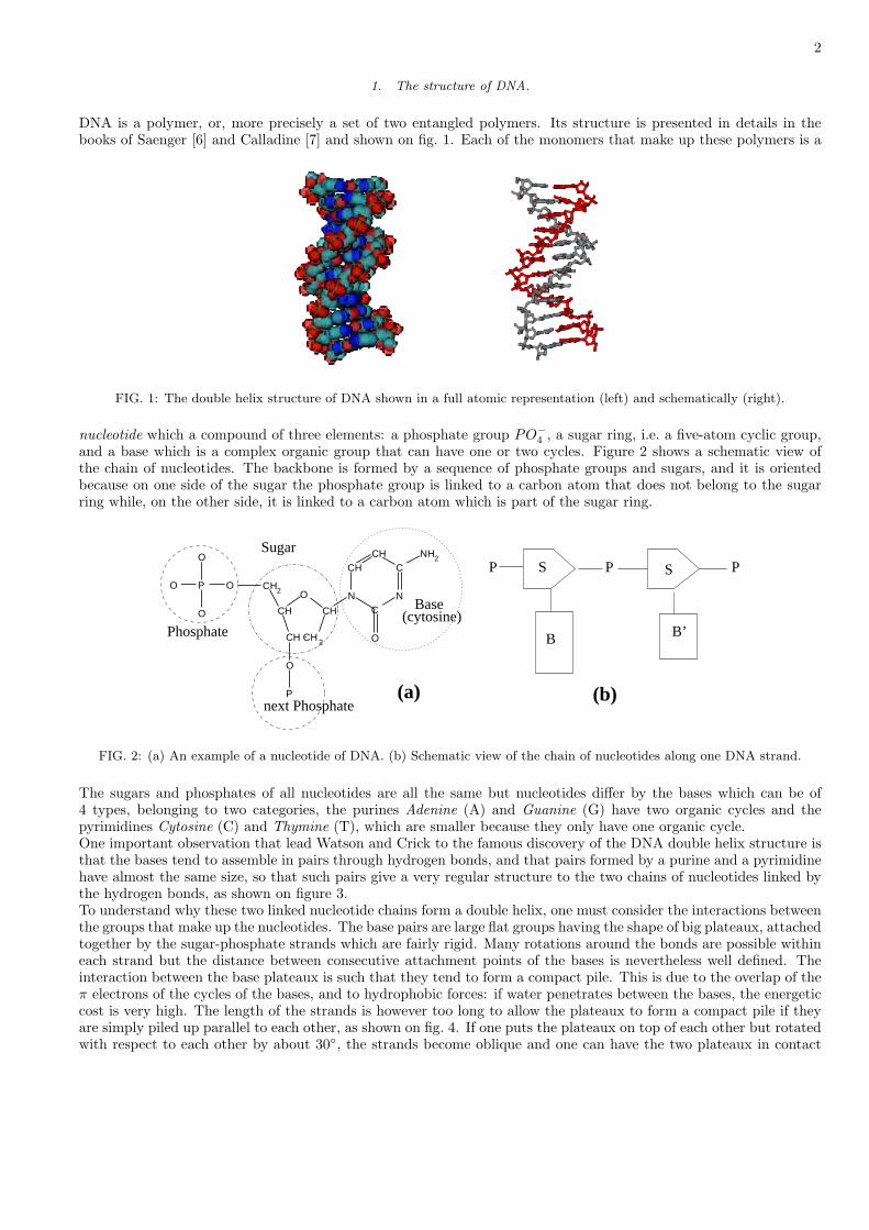
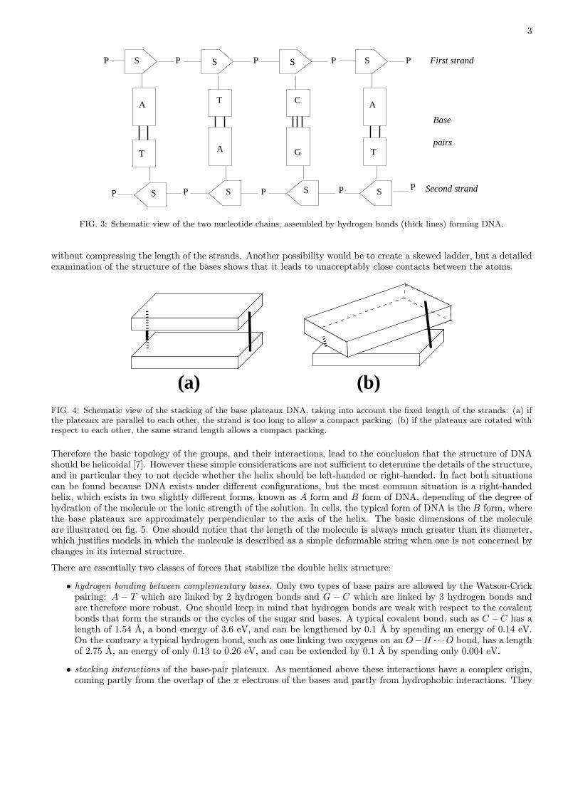
The sugars and phosphates of all nucleotides are all the same but nucleotides differ by the bases which can be of4 types, belonging to two categories, the purines Adenine (A) and Guanine (G) have two organic cycles and thepyrimidines Cytosine (C) and Thymine (T), which are smaller because they only have one organic cycle.One important observation that lead Watson and Crick to the famous discovery of the DNA double helix structure isthat the bases tend to assemble in pairs through hydrogen bonds, and that pairs formed by a purine and a pyrimidinehave almost the same size, so that such pairs give a very regular structure to the two chains of nucleotides linked bythe hydrogen bonds, as shown on figure 3.To understand why these two linked nucleotide chains form a double helix, one must consider the interactions betweenthe groups that make up the nucleotides. The base pairs are large flat groups having the shape of big plateaux, attachedtogether by the sugar-phosphate strands which are fairly rigid. Many rotations around the bonds are possible withineach strand but the distance between consecutive attachment points of the bases is nevertheless well defined. Theinteraction between the base plateaux is such that they tend to form a compact pile. This is due to the overlap of theπ electrons of the cycles of the bases, and to hydrophobic forces: if water penetrates between the bases, the energeticcost is very high. The length of the strands is however too long to allow the plateaux to form a compact pile if theyare simply piled up parallel to each other, as shown on fig. 4. If one puts the plateaux on top of each other but rotatedwith respect to each other by about 30◦, the strands become oblique and one can have the two plateaux in contact

3

PS

A

PSP S P S P

A T C

P P P PP S S S S

T A G T

Base

pairs

Second strand

First strand

FIG. 3: Schematic view of the two nucleotide chains, assembled by hydrogen bonds (thick lines) forming DNA.

without compressing the length of the strands. Another possibility would be to create a skewed ladder, but a detailedexamination of the structure of the bases shows that it leads to unacceptably close contacts between the atoms.

(a) (b)FIG. 4: Schematic view of the stacking of the base plateaux DNA, taking into account the fixed length of the strands: (a) ifthe plateaux are parallel to each other, the strand is too long to allow a compact packing. (b) if the plateaux are rotated withrespect to each other, the same strand length allows a compact packing.

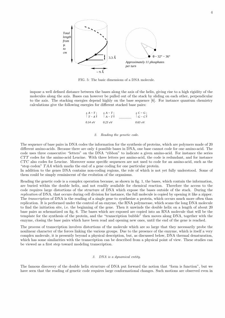
Therefore the basic topology of the groups, and their interactions, lead to the conclusion that the structure of DNAshould be helicoidal [7]. However these simple considerations are not sufficient to determine the details of the structure,and in particular they to not decide whether the helix should be left-handed or right-handed. In fact both situationscan be found because DNA exists under different configurations, but the most common situation is a right-handedhelix, which exists in two slightly different forms, known as A form and B form of DNA, depending of the degree ofhydration of the molecule or the ionic strength of the solution. In cells, the typical form of DNA is the B form, wherethe base plateaux are approximately perpendicular to the axis of the helix. The basic dimensions of the moleculeare illustrated on fig. 5. One should notice that the length of the molecule is always much greater than its diameter,which justifies models in which the molecule is described as a simple deformable string when one is not concerned bychanges in its internal structure.

There are essentially two classes of forces that stabilize the double helix structure:

• hydrogen bonding between complementary bases. Only two types of base pairs are allowed by the Watson-Crickpairing: A − T which are linked by 2 hydrogen bonds and G − C which are linked by 3 hydrogen bonds andare therefore more robust. One should keep in mind that hydrogen bonds are weak with respect to the covalentbonds that form the strands or the cycles of the sugar and bases. A typical covalent bond, such as C −C has alength of 1.54 A, a bond energy of 3.6 eV, and can be lengthened by 0.1 A by spending an energy of 0.14 eV.On the contrary a typical hydrogen bond, such as one linking two oxygens on an O−H · · ·O bond, has a lengthof 2.75 A, an energy of only 0.13 to 0.26 eV, and can be extended by 0.1 A by spending only 0.004 eV.

• stacking interactions of the base-pair plateaux. As mentioned above these interactions have a complex origin,coming partly from the overlap of the π electrons of the bases and partly from hydrophobic interactions. They

4

3.3 A

~ 9 A

~ 32° − 36°°

°

lengthTotal

from

tocm

µ

θ

Approximately 11 phosphatesper turn

FIG. 5: The basic dimensions of a DNA molecule.

impose a well defined distance between the bases along the axis of the helix, giving rise to a high rigidity of themolecules along the axis. Bases can however be pulled out of the stack by sliding on each other, perpendicularto the axis. The stacking energies depend highly on the base sequence [6]. For instance quantum chemistrycalculations give the following energies for different stacked base pairs:

.................

A − T

eV eV

A − TC − GG − C

0.23 0.63

A − TT − A

0.14 eV

2. Reading the genetic code.

The sequence of base pairs in DNA codes the information for the synthesis of proteins, which are polymers made of 20different amino-acids. Because there are only 4 possible bases in DNA, one base cannot code for one amino-acid. Thecode uses three consecutive “letters” on the DNA “ribbon” to indicate a given amino-acid. For instance the seriesCTT codes for the amino-acid Leucine. With three letters per amino-acid, the code is redundant, and for instanceCTC also codes for Leucine. Moreover some specific sequences are not used to code for an amino-acid, such as the“stop codon” TAA which marks the end of a gene coding for one particular protein.In addition to the genes DNA contains non-coding regions, the role of which is not yet fully understood. Some ofthem could be simply reminiscent of the evolution of the organisms.

Reading the genetic code is a complex operation because, as shown in fig. 1, the bases, which contain the information,are buried within the double helix, and not readily available for chemical reaction. Therefore the access to thecode requires large distortions of the structure of DNA which expose the bases outside of the stack. During thereplication of DNA, that occurs during cell division for instance, the full molecule is copied by opening it like a zipper.The transcription of DNA is the reading of a single gene to synthesize a protein, which occurs much more often thanreplication. It is performed under the control of an enzyme, the RNA polymerase, which scans the long DNA moleculeto find the initiation site, i.e. the beginning of the gene. Then it unwinds the double helix on a length of about 20base pairs as schematized on fig. 6. The bases which are exposed are copied into an RNA molecule that will be thetemplate for the synthesis of the protein, and the “transcription bubble” then moves along DNA, together with theenzyme, closing the base pairs which have been read and opening new ones, until the end of the gene is reached.

The process of transcription involves distortions of the molecule which are so large that they necessarily probe thenonlinear character of the forces linking the various groups. Due to the presence of the enzyme, which is itself a verycomplex molecule, it is presently beyond a physical description, but, as discussed below, DNA thermal denaturation,which has some similarities with the transcription can be described from a physical point of view. These studies canbe viewed as a first step toward modeling transcription.

3. DNA is a dynamical entity.

The famous discovery of the double helix structure of DNA put forward the notion that “form is function”, but wehave seen that the reading of genetic code requires large conformational changes. Such motions are observed even in

5

Replication

ARNpolymérase

ARN

Transcription

FIG. 6: Schematic picture of the replication and transcription of DNA.

the absence of enzymes. DNA is a highly dynamical entity and its structure is not frozen. The “breathing” of DNAhas been known from biologists for decades. It consists in the temporary opening of the base pairs. This is attestedby proton-deuterium exchange experiments. DNA is put in solution in deuterated water, and one observes that theimino-protons, which are the protons forming hydrogen bonds between two bases in a base pair, are exchanged withdeuterium coming from the solvent. As these protons are deeply buried in the DNA structure, the exchange indicatesthat bases can open, at least temporarily, to expose the imino protons to the solvent [8]. The determination of thelifetime of a base pair, i.e. the time during which it stays closed, has been the subject of some controversy [9] becausethe rate limiting step in the exchange may be either the rate at which base pairs open, or the time necessary for theexchange. Accurate experiments, using NMR to detect the exchange, showed that the lifetime of a base pair is of theorder of 10 ms. These experiments also show that the protons of one particular base pair can be exchanged whilethose of a base pair next to it are not exchanged. This indicates that the large conformational changes that lead tobase pair opening in DNA are highly localized, which means that the coupling between successive bases along theDNA helix is weak enough to allow consecutive bases to move almost independently from each other.

B. Physical experiments on DNA.

To model the nonlinear dynamics of DNA, one needs precise data to establish a meaningful model. They are providedby various physical experiments. Many data have been obtained by standard methods of condensed matter physics,but, in the last few years, powerful new methods appeared, based on single molecule experiments.

1. Experiments based on standard methods of solid state physics.

The static structure of DNA is obtained by standard X-ray or neutron diffraction. It is the earlier X-ray investigationsof Rosalind Franklin, showing patterns characteristic of a helix, that put Watson and Crick on the track leading totheir discovery of the double helix structure. Since then the accuracy of the determinations have been considerablyimproved and the structure of DNA is known to a high precision [6].Dynamical data can be obtained by infra-red or Raman vibrational spectroscopy [10, 11], or by quasi-elastic or inelasticneutron scattering which allow a complete exploration of the dispersion curves of the small vibrational modes of DNA[12].The main difficulty in all these experiments is to obtain oriented samples. DNA segments of a few tens of base pairscan form small crystals. Neutron diffraction need much larger samples, which can be obtained by a rather remarkablemethod [12]: using natural DNA molecules a few micron long, the addition of alcohol leads to the precipitation ofDNA fibers. A spinning method can be used to get a “DNA wire” from these fibers. The “wire” is rolled around acylinder, leading to a sheet of parallel DNA fibers. Many of these sheets can then be mounted in a sample holder togive a sufficient volume of oriented DNA molecule. This technique is remarkable by its ability to manipulate molecules,but it also raises interesting theoretical questions. The precipitation of DNA into fibers is due to electrostatic forcesbut it is not fully understood presently [13].

6

60° C 70°C

UV

Abs

orpt

ion

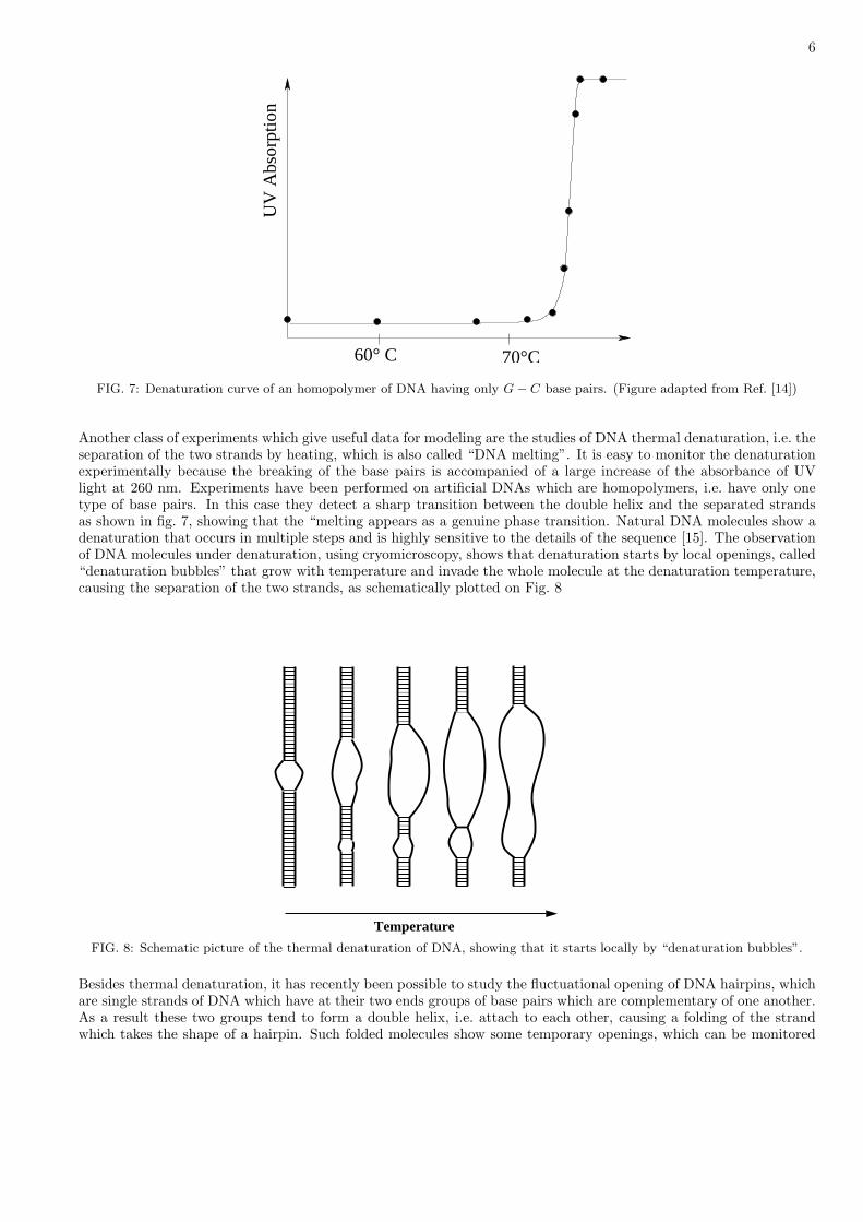
FIG. 7: Denaturation curve of an homopolymer of DNA having only G− C base pairs. (Figure adapted from Ref. [14])

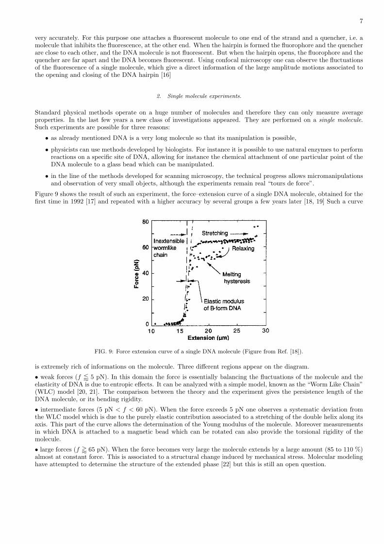
Another class of experiments which give useful data for modeling are the studies of DNA thermal denaturation, i.e. theseparation of the two strands by heating, which is also called “DNA melting”. It is easy to monitor the denaturationexperimentally because the breaking of the base pairs is accompanied of a large increase of the absorbance of UVlight at 260 nm. Experiments have been performed on artificial DNAs which are homopolymers, i.e. have only onetype of base pairs. In this case they detect a sharp transition between the double helix and the separated strandsas shown in fig. 7, showing that the “melting appears as a genuine phase transition. Natural DNA molecules show adenaturation that occurs in multiple steps and is highly sensitive to the details of the sequence [15]. The observationof DNA molecules under denaturation, using cryomicroscopy, shows that denaturation starts by local openings, called“denaturation bubbles” that grow with temperature and invade the whole molecule at the denaturation temperature,causing the separation of the two strands, as schematically plotted on Fig. 8

Temperature

FIG. 8: Schematic picture of the thermal denaturation of DNA, showing that it starts locally by “denaturation bubbles”.

Besides thermal denaturation, it has recently been possible to study the fluctuational opening of DNA hairpins, whichare single strands of DNA which have at their two ends groups of base pairs which are complementary of one another.As a result these two groups tend to form a double helix, i.e. attach to each other, causing a folding of the strandwhich takes the shape of a hairpin. Such folded molecules show some temporary openings, which can be monitored

7

very accurately. For this purpose one attaches a fluorescent molecule to one end of the strand and a quencher, i.e. amolecule that inhibits the fluorescence, at the other end. When the hairpin is formed the fluorophore and the quencherare close to each other, and the DNA molecule is not fluorescent. But when the hairpin opens, the fluorophore and thequencher are far apart and the DNA becomes fluorescent. Using confocal microscopy one can observe the fluctuationsof the fluorescence of a single molecule, which give a direct information of the large amplitude motions associated tothe opening and closing of the DNA hairpin [16]

2. Single molecule experiments.

Standard physical methods operate on a huge number of molecules and therefore they can only measure averageproperties. In the last few years a new class of investigations appeared. They are performed on a single molecule.Such experiments are possible for three reasons:

• as already mentioned DNA is a very long molecule so that its manipulation is possible,

• physicists can use methods developed by biologists. For instance it is possible to use natural enzymes to performreactions on a specific site of DNA, allowing for instance the chemical attachment of one particular point of theDNA molecule to a glass bead which can be manipulated.

• in the line of the methods developed for scanning microscopy, the technical progress allows micromanipulationsand observation of very small objects, although the experiments remain real “tours de force”.

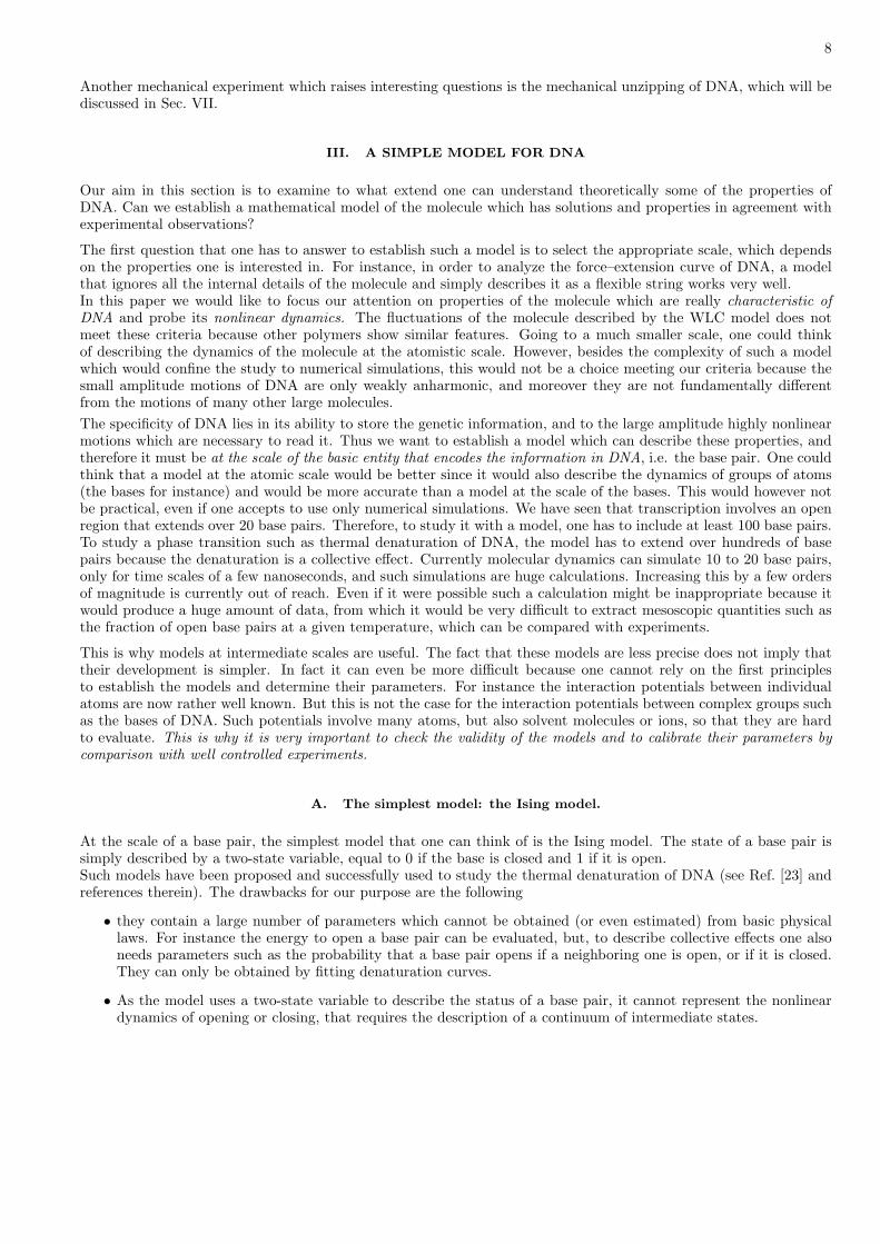
Figure 9 shows the result of such an experiment, the force–extension curve of a single DNA molecule, obtained for thefirst time in 1992 [17] and repeated with a higher accuracy by several groups a few years later [18, 19] Such a curve

FIG. 9: Force extension curve of a single DNA molecule (Figure from Ref. [18]).

is extremely rich of informations on the molecule. Three different regions appear on the diagram.

• weak forces (f / 5 pN). In this domain the force is essentially balancing the fluctuations of the molecule and theelasticity of DNA is due to entropic effects. It can be analyzed with a simple model, known as the “Worm Like Chain”(WLC) model [20, 21]. The comparison between the theory and the experiment gives the persistence length of theDNA molecule, or its bending rigidity.

• intermediate forces (5 pN < f < 60 pN). When the force exceeds 5 pN one observes a systematic deviation fromthe WLC model which is due to the purely elastic contribution associated to a stretching of the double helix along itsaxis. This part of the curve allows the determination of the Young modulus of the molecule. Moreover measurementsin which DNA is attached to a magnetic bead which can be rotated can also provide the torsional rigidity of themolecule.

• large forces (f ' 65 pN). When the force becomes very large the molecule extends by a large amount (85 to 110 %)almost at constant force. This is associated to a structural change induced by mechanical stress. Molecular modelinghave attempted to determine the structure of the extended phase [22] but this is still an open question.

8

Another mechanical experiment which raises interesting questions is the mechanical unzipping of DNA, which will bediscussed in Sec. VII.

III. A SIMPLE MODEL FOR DNA

Our aim in this section is to examine to what extend one can understand theoretically some of the properties ofDNA. Can we establish a mathematical model of the molecule which has solutions and properties in agreement withexperimental observations?

The first question that one has to answer to establish such a model is to select the appropriate scale, which dependson the properties one is interested in. For instance, in order to analyze the force–extension curve of DNA, a modelthat ignores all the internal details of the molecule and simply describes it as a flexible string works very well.In this paper we would like to focus our attention on properties of the molecule which are really characteristic ofDNA and probe its nonlinear dynamics. The fluctuations of the molecule described by the WLC model does notmeet these criteria because other polymers show similar features. Going to a much smaller scale, one could thinkof describing the dynamics of the molecule at the atomistic scale. However, besides the complexity of such a modelwhich would confine the study to numerical simulations, this would not be a choice meeting our criteria because thesmall amplitude motions of DNA are only weakly anharmonic, and moreover they are not fundamentally differentfrom the motions of many other large molecules.The specificity of DNA lies in its ability to store the genetic information, and to the large amplitude highly nonlinearmotions which are necessary to read it. Thus we want to establish a model which can describe these properties, andtherefore it must be at the scale of the basic entity that encodes the information in DNA, i.e. the base pair. One couldthink that a model at the atomic scale would be better since it would also describe the dynamics of groups of atoms(the bases for instance) and would be more accurate than a model at the scale of the bases. This would however notbe practical, even if one accepts to use only numerical simulations. We have seen that transcription involves an openregion that extends over 20 base pairs. Therefore, to study it with a model, one has to include at least 100 base pairs.To study a phase transition such as thermal denaturation of DNA, the model has to extend over hundreds of basepairs because the denaturation is a collective effect. Currently molecular dynamics can simulate 10 to 20 base pairs,only for time scales of a few nanoseconds, and such simulations are huge calculations. Increasing this by a few ordersof magnitude is currently out of reach. Even if it were possible such a calculation might be inappropriate because itwould produce a huge amount of data, from which it would be very difficult to extract mesoscopic quantities such asthe fraction of open base pairs at a given temperature, which can be compared with experiments.

This is why models at intermediate scales are useful. The fact that these models are less precise does not imply thattheir development is simpler. In fact it can even be more difficult because one cannot rely on the first principlesto establish the models and determine their parameters. For instance the interaction potentials between individualatoms are now rather well known. But this is not the case for the interaction potentials between complex groups suchas the bases of DNA. Such potentials involve many atoms, but also solvent molecules or ions, so that they are hardto evaluate. This is why it is very important to check the validity of the models and to calibrate their parameters bycomparison with well controlled experiments.

A. The simplest model: the Ising model.

At the scale of a base pair, the simplest model that one can think of is the Ising model. The state of a base pair issimply described by a two-state variable, equal to 0 if the base is closed and 1 if it is open.Such models have been proposed and successfully used to study the thermal denaturation of DNA (see Ref. [23] andreferences therein). The drawbacks for our purpose are the following

• they contain a large number of parameters which cannot be obtained (or even estimated) from basic physicallaws. For instance the energy to open a base pair can be evaluated, but, to describe collective effects one alsoneeds parameters such as the probability that a base pair opens if a neighboring one is open, or if it is closed.They can only be obtained by fitting denaturation curves.

• As the model uses a two-state variable to describe the status of a base pair, it cannot represent the nonlineardynamics of opening or closing, that requires the description of a continuum of intermediate states.

9

B. A simple model for nonlinear DNA dynamics.

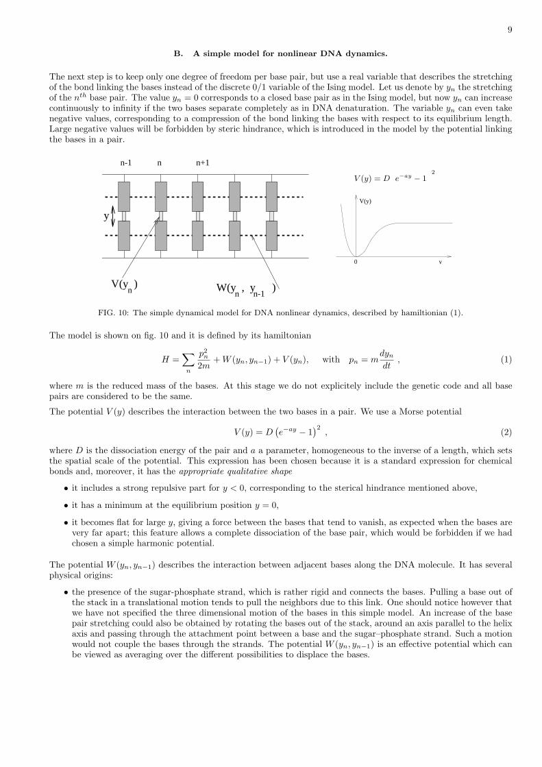
The next step is to keep only one degree of freedom per base pair, but use a real variable that describes the stretchingof the bond linking the bases instead of the discrete 0/1 variable of the Ising model. Let us denote by yn the stretchingof the nth base pair. The value yn = 0 corresponds to a closed base pair as in the Ising model, but now yn can increasecontinuously to infinity if the two bases separate completely as in DNA denaturation. The variable yn can even takenegative values, corresponding to a compression of the bond linking the bases with respect to its equilibrium length.Large negative values will be forbidden by steric hindrance, which is introduced in the model by the potential linkingthe bases in a pair.

n n+1n-1

V(y )n W(y , y )

n n-1

y

V (y) = Dşe−ay − 1

ť2

V(y)

0 y

FIG. 10: The simple dynamical model for DNA nonlinear dynamics, described by hamiltionian (1).

The model is shown on fig. 10 and it is defined by its hamiltonian

H =∑

n

p2n

2m+ W (yn, yn−1) + V (yn), with pn = m

dyn

dt, (1)

where m is the reduced mass of the bases. At this stage we do not explicitely include the genetic code and all basepairs are considered to be the same.

The potential V (y) describes the interaction between the two bases in a pair. We use a Morse potential

V (y) = D(e−ay − 1

)2, (2)

where D is the dissociation energy of the pair and a a parameter, homogeneous to the inverse of a length, which setsthe spatial scale of the potential. This expression has been chosen because it is a standard expression for chemicalbonds and, moreover, it has the appropriate qualitative shape

• it includes a strong repulsive part for y < 0, corresponding to the sterical hindrance mentioned above,

• it has a minimum at the equilibrium position y = 0,

• it becomes flat for large y, giving a force between the bases that tend to vanish, as expected when the bases arevery far apart; this feature allows a complete dissociation of the base pair, which would be forbidden if we hadchosen a simple harmonic potential.

The potential W (yn, yn−1) describes the interaction between adjacent bases along the DNA molecule. It has severalphysical origins:

• the presence of the sugar-phosphate strand, which is rather rigid and connects the bases. Pulling a base out ofthe stack in a translational motion tends to pull the neighbors due to this link. One should notice however thatwe have not specified the three dimensional motion of the bases in this simple model. An increase of the basepair stretching could also be obtained by rotating the bases out of the stack, around an axis parallel to the helixaxis and passing through the attachment point between a base and the sugar–phosphate strand. Such a motionwould not couple the bases through the strands. The potential W (yn, yn−1) is an effective potential which canbe viewed as averaging over the different possibilities to displace the bases.

10

• the direct interaction between the base pair plateaux, which is due to an overlap of the π-electron orbitals ofthe organic rings that make up the bases.

In a first stage, we shall use for W (yn, yn−1) the simplest expression, i.e. the expansion of the potential around itsminimum which is reached when yn = yn−1

W (yn, yn−1) =12K(yn − yn−1)2 . (3)

Such an harmonic approximation would be good if the stacking interaction were strong enough to keep yn close toyn−1 at all times. This is not true for DNA, but the harmonic approximation allows easier calculations, and it issufficient to get some interesting results which agree with some experimental observations. However we shall see thatthe expression of W has to be improved to provide a correct description of the thermal denaturation.

The choice of the potential parameters is a very difficult question because, as discussed above, the potentials entering inthe model are effective potentials, which combine many actual interactions. For instance V (y) includes the hydrogenbonds between the bases but also the repulsion between the charged phosphate groups, which is partly screened bythe ions which are in solutions.The parameter that we use have been calibrated by comparison with experiments, in particular the thermal denatu-ration as discussed in Sec. VI, but they are not accurately known. The parameters for V (y) are D = 0.03 eV, whichis slightly above kBT at room temperature (kB being the Boltzmann constant) and a = 4.5 A−1. For a stretching ofthe base pair distance of 0.1 A, these parameters give a variation of energy of 0.006 eV, which is consistent with thevalues that we listed for hydrogen bonds in Sec. II. The value chosen for K is K = 0.06 eV/A2, which corresponds toa weak coupling between the bases, as attested by the experimental results showing that proton-deuterium exchangecan occur on one base pair without affecting the neighbors. The average mass of the nucleotides is 300 atomic massunits.

The values of the constants have been given with a systems of units adapted to the scale of the problem: lengths inunits of ` = 1 A, energies in units of e = 1 eV, mass in units of m0 = 1 atomic mass unit. This defines a naturaltime unit t0 through e = m0 `2 t−2

0 , which is equal to t0 = 1.018 10−14 s, which is of the order of magnitude of theperiod of the vibrational motions of the base pairs.

Although actual units are important to compare the results with experiments, for theoretical calculations, it is veryuseful to express the problem in terms of dimensionless quantities. It is natural to introduce the dimensionlessstretching of the base pairs as Y = ay. If we measure the energies in units of the depth D of the Morse potential, thedimensionless hamiltonian is H ′ = H/D, and defining the dimensionless quantity S = K/(Da2), and a dimensionlesstime τ =

√Da2/mt , we obtain the hamiltonian H ′ only in terms of dimensionless quantities under the form

H ′ =∑

n

12P 2

n +12S(Yn − Yn−1)2 +

(e−Yn − 1

)2with Pn =

dYn

dτ, (4)

from which one can derive dimensionless equations of motion, which depend on a single parameter S which is equalto S = 0.0976 with our potential parameters.

IV. OBSERVING THE DYNAMICS OF THE DNA MODEL.

A simple method to evaluate the ability of this model to describe DNA is to observe its dynamics and compare itwith the experimental properties of DNA. Numerical simulations can be used, but for meaningful comparisons withwith actual properties of the molecule, they must take into account thermal fluctuations.

A. Methods for molecular dynamics at constant temperature.

Simulating a thermal bath is not a simple task, but several methods have been designed to satisfactorily approximatethe thermal fluctuations. A simple one is to add to the equations of motions a fluctuating force and a damping term,related by the fluctuation dissipation theorem, leading to a set of coupled Langevin equations. A more efficient wayhas been developed by Nose [24] and improved by Martyna et al. [25]. The idea is to simulate an extended systemwhich includes not only the physical system of interest but a few additional dynamical variables corresponding toa chain of “thermostats”. One of the thermostats is coupled to all the degrees of freedom of the physical system,

11

according to the method proposed by Nose that leads to exact canonical properties for the physical system, and theothers contribute to properly randomize the first thermostat in order to ensure a proper exploration of the phasespace of the system. This approach leads to a faster thermalization than Langevin simulations and one can controlthat, not only the average kinetic energy corresponds to the expected temperature, but also the fluctuations of thekinetic energy have the value N(kBT )2 expected for a one dimensional canonical system with N degrees of freedom.

B. Dynamics of the thermalized nonlinear DNA model.

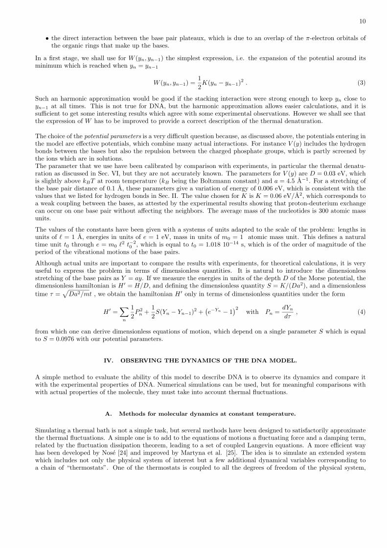
Figure 11 shows two typical results of the numerical simulation of the dynamics of a 256-base-pair segment of theDNA model in contact with a thermal bath.

(a) (b)

Tim

e

Tem

per

atu

re/T

ime

1 . . . n . . . 256 1 . . . n . . . 256

FIG. 11: Numerical simulations of the dynamics of the DNA model in contact with a thermal bath simulated according tothe method of Martyna et al. [25]. The model has 256 base pairs. The amplitude of the base pair stretching is shown by agray scale ranging from white (base pair fully closed) to black (base pair completely open). The horizontal axis extends alongthe molecule and the vertical axis corresponds to time (and temperature when we use a temperature ramp). (a) Simulation atconstant temperature T = 340 K. (b) Simulation performed with a linear temperature ramp, corresponding to a denaturationexperiment where temperature is continuously raised from low T to a temperature beyond denaturation.

Fig. 11.a shows a case where the model is kept at constant temperature T = 340 K, which is slightly below thedenaturation temperature. It displays two types of characteristic patterns. The most apparent are large black spots,which correspond to regions where the base pair stretching is very large over a few tens of consecutive bases for alimited time. Such regions correspond to the “denaturation bubbles” observed in the experiments. Another noticeablefeature is the presence of vertical dotted lines, i.e. successions of black and white regions involving a few base pairs,located in one particular place of DNA. Such patterns are created by very large amplitude localized vibrational modesof the molecule, and could correspond to the “breathing of DNA” observed in experiments.

12

The simulation also points out an interesting feature of the model, which is an actual DNA property: the existence oflocalized large amplitude motions appears as a temporary breaking of energy equipartition in the system, although itis in equilibrium. Figure 11.a clearly shows regions where the displacements are large separated by narrower “cold”regions where the fluctuations of the base pairs are much smaller. Of course energy equipartition is indeed obeyed,but to observe it one must follow the dynamics on very long time scales. On times which can be as large as thousandsof periods of the small amplitude vibrations of the bases, one finds “hot regions” coexisting with “cold regions”, but,on even longer times, the amplitude of the fluctuations in some hot regions will decrease while they grow in someother regions. A true uniformity in the fluctuations is never achieved but the inhomogeneities move from place toplace. This phenomenon is reminiscent of turbulence, where pressure in a fluid shows large local fluctuations althoughan average pressure can be well defined. And a quantitative analysis of the properties of a lattice of coupled nonlinearoscillators shows that the relationship with turbulence may go well beyond a simple qualitative analogy [26].

Figure 11.b shows the results of a simulation that mimics an actual denaturation experiment: the temperature israised in a linear manner from a low value to a value slightly beyond the denaturation temperature. Such a numericalexperiment can only give a crude picture of the denaturation process because, in order to keep the simulation withinthe times accessible to molecular dynamics, the heating has to be achieved in a few nanoseconds, which means that thesystem is strongly out of equilibrium. However such a calculation gives an idea of the actual denaturation process andit shows that the model gives results which are in good agreement with the observations (see Fig. 8): the denaturationis preceeded by the formation of large open regions, that grow quickly when the denaturation temperature approaches,until they invade the whole sample, causing the separation of the strands. Moreover the simulation shows that thelocalized modes described above appear as the precursors of the formation of the bubbles.

V. NONLINEAR EXCITATIONS IN DNA: BREATHERS AND DOMAIN WALLS.

Let us now try to get some analytical understanding of the numerical observations discussed in the previous section.

A. Derivation of a nonlinear equation for the model

The starting point is the equations of motions of the model that derive from hamiltonian (4)

d2Yn

dτ2= S(Yn+1 + Yn−1 − 2Yn) + 2 e−Yn

(e−Yn − 1

)= 0 . (5)

They form a set of coupled nonlinear differential equations which cannot be solved exactly. The simulations showthat, even at low temperature, the stretching of the base pairs can become large in some regions and therefore anharmonic approximation has to be ruled out. We can however introduce a small amplitude expansion that keeps thefirst nonlinearities by defining

Yn = εφn avec ε ¿ 1 , (6)

and keeping only the leading terms in the expansion

d2φn

dτ2= S(φn+1 + φn−1 − 2φn)− 2

(φn − 3

2εφ2

n +76ε2φ3

n

)= 0 . (7)

One can look for a solution of this set of equations, which extends the simple plane wave solution that we would getin a linear approximation, under the form

φn(τ) =(Fneiθn + F ?

ne−iθn)

+ ε(Gn + Hne2iθn + H?

ne−2iθn)

, (8)

with θn = qn−ωt. The choice of the additional terms will be justified more precisely later but it is easy to understandtheir origin: as the equations contain a term εφ2

n, the presence of the dominant term in solution (8) proportional toexp(±iθn) will naturally generate terms similar to the factor ε in the solution, i.e. without ann exponential contributionor depending on exp(±2iθn). Moreover, as the solution (8) appears as a modulated plane wave, which, in the harmoniclimit would keep a fixed amplitude, it is natural to assume that the coefficients Fn, Gn, Hn will only have a smoothspatial dependence when nonlinearity is included. These functions are assumed to depend only on “slow” variablesX1 = εx, X2 = ε2x, T1 = ετ , T2 = ε2τ , and their spatial dependence is then rather well described by a continuumlimit approximation, which amounts to replacing the functions at sites n± 1 by their Taylor expansion

Fn±1 = F ± ε∂F

∂X1± ε2

∂F

∂X2+

ε2

2∂2F

∂X21

. (9)

13

The time derivatives of these functions are of the form

∂Fn

∂τ= ε

∂F

∂T1+ ε2

∂F

∂T2, (10)

with similar equations for G and H. Putting these expressions in the equations of motion, at order ε0 the cancellationof terms in exp(±iθn) shows that the equations are satisfied if ω and q are linked by the dispersion relation that onegets for plane waves the harmonic limit

ω2 = 2 + 4S sin2 q

2. (11)

Notice that this dispersion relation corresponds to the discrete lattice, i.e. in spite of the continuum limit approximationperformed for the envelope functions F , G, H, the calculation preserves some discreteness, which is important forDNA. This is why this approximation is called the semi-discrete approximation [27].

At order ε1, the cancellation of terms in exp(±iθn) gives

∂F

∂T1+ vg

∂F

∂X1= 0 where vg =

S sin q

ω, (12)

is the group velocity of the waves having the dispersion relation (11). At the same order, terms without an exponentialdependence and terms in exp(2iθn) give

G = 3F F ? H = −12

F 2

1 + (8S/3) sin4 (q/2). (13)

One can notice that the G and H terms in solution (8) are necessary to allow the cancellation of the terms of orderε1 in the equations of motion.

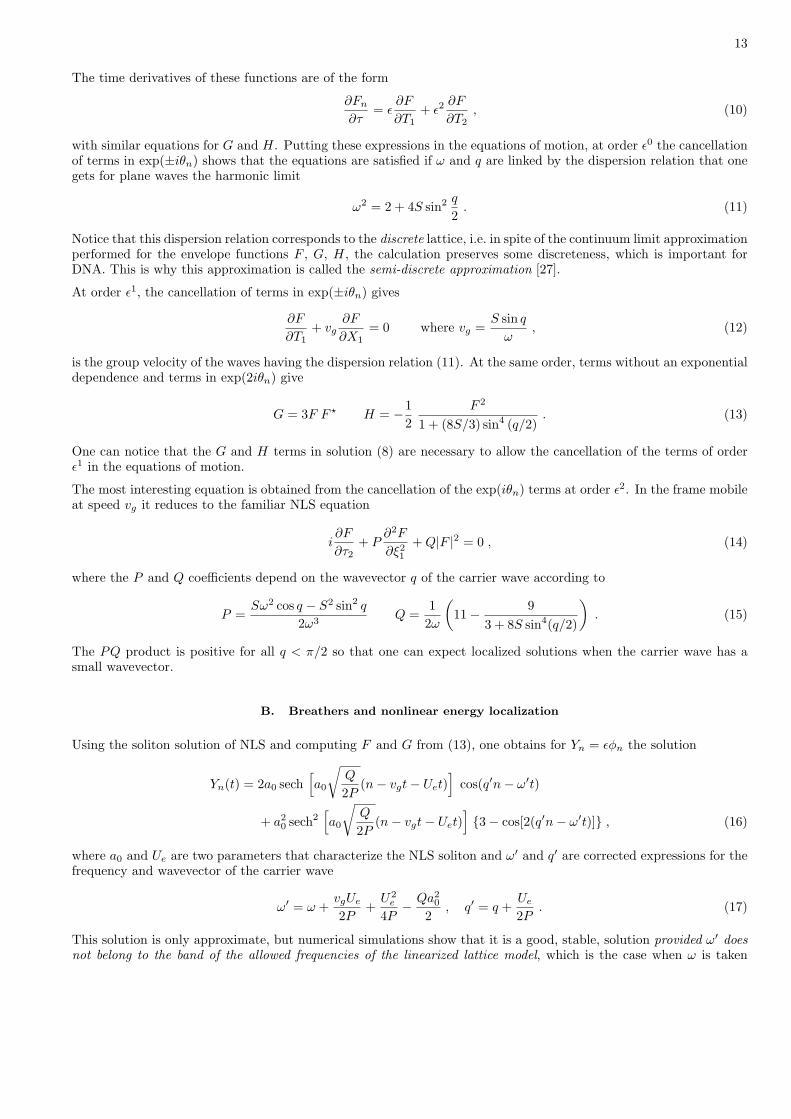
The most interesting equation is obtained from the cancellation of the exp(iθn) terms at order ε2. In the frame mobileat speed vg it reduces to the familiar NLS equation

i∂F

∂τ2+ P

∂2F

∂ξ21

+ Q|F |2 = 0 , (14)

where the P and Q coefficients depend on the wavevector q of the carrier wave according to

P =Sω2 cos q − S2 sin2 q

2ω3Q =

12ω

(11− 9

3 + 8S sin4(q/2)

). (15)

The PQ product is positive for all q < π/2 so that one can expect localized solutions when the carrier wave has asmall wavevector.

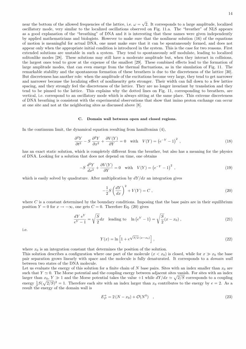
B. Breathers and nonlinear energy localization

Using the soliton solution of NLS and computing F and G from (13), one obtains for Yn = εφn the solution

Yn(t) = 2a0 sech[a0

√Q

2P(n− vgt− Uet)

]cos(q′n− ω′t)

+ a20 sech2

[a0

√Q

2P(n− vgt− Uet)

]{3− cos[2(q′n− ω′t)]} , (16)

where a0 and Ue are two parameters that characterize the NLS soliton and ω′ and q′ are corrected expressions for thefrequency and wavevector of the carrier wave

ω′ = ω +vgUe

2P+

U2e

4P− Qa2

0

2, q′ = q +

Ue

2P. (17)

This solution is only approximate, but numerical simulations show that it is a good, stable, solution provided ω′ doesnot belong to the band of the allowed frequencies of the linearized lattice model, which is the case when ω is taken

14

near the bottom of the allowed frequencies of the lattice, i.e. ω =√

2. It corresponds to a large amplitude, localizedoscillatory mode, very similar to the localized oscillations observed on Fig. 11.a. The “breather” of NLS appearsas a good explanation of the “breathing” of DNA and it is interesting that these names were given independentlyby applied mathematicians and biologists. However to make sure that the nonlinear solution (16) of the equationsof motion is meaningful for actual DNA, one must make sure that it can be spontaneously formed, and does notappear only when the appropriate initial condition is introduced in the system. This is the case for two reasons. Firstextended solutions are unstable in such a system. They tend to spontaneously self modulate, leading to localizedsolitonlike modes [28]. These solutions may still have a moderate amplitude but, when they interact in collisions,the largest ones tend to grow at the expense of the smallest [29]. These combined effects lead to the formation oflarge amplitude modes, that can even emerge from the thermal fluctuations, as in the simulation of Fig. 11. Theremarkable stability and the spontaneous formation of these breathers is due to the discreteness of the lattice [30].But discreteness has another role: when the amplitude of the excitations become very large, they tend to get narrowerand narrower because the localizing effect of nonlinearity gets stronger. Their width can fall down to a few latticespacing, and they strongly feel the discreteness of the lattice. They are no longer invariant by translation and theytend to be pinned to the lattice. This explains why the dotted lines on Fig. 11, corresponding to breathers, arevertical, i.e. correspond to an oscillatory mode which is always sitting at the same place. This extreme discretenessof DNA breathing is consistent with the experimental observations that show that imino proton exchange can occurat one site and not at the neighboring sites as discussed above [8].

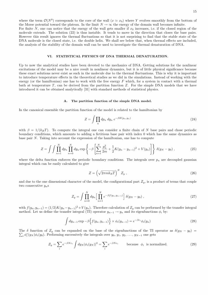
C. Domain wall between open and closed regions.

In the continuum limit, the dynamical equation resulting from hamiltonian (4),

∂2Y

∂t2− S

∂2Y

∂x2+

∂V (Y )∂Y

= 0 with V (Y ) =(e−Y − 1

)2, (18)

has an exact static solution, which is completely different from the breather, but also has a meaning for the physicsof DNA. Looking for a solution that does not depend on time, one obtains

−Sd2Y

dx2+

∂V (Y )∂Y

= 0 with V (Y ) =(e−Y − 1

)2, (19)

which is easily solved by quadrature. After multiplication by dY/dx an integration gives

−12S

(dY

dx

)2

+ V (Y ) = C , (20)

where C is a constant determined by the boundary conditions. Imposing that the base pairs are in their equilibriumposition Y = 0 for x → −∞, one gets C = 0. Therefore Eq. (20) gives

dY eY

eY − 1=

√S

2dx leading to ln

(eY − 1

)=

√S

2(x− x0) , (21)

i.e.

Y (x) = ln[1 + e

√S/2 (x−x0)

], (22)

where x0 is an integration constant that determines the position of the solution.This solution describes a configuration where one part of the molecule (x < x0) is closed, while for x À x0 the basepair separation grows linearly with space and the molecule is fully denaturated. It corresponds to a domain wallbetween two states of the DNA molecule.Let us evaluate the energy of this solution for a finite chain of N base pairs. Sites with an index smaller than x0 aresuch that Y ' 0. The Morse potential and the coupling energy between adjacent sites vanish. For sites with an indexlarger than x0, Y À 1 and the Morse potential takes the value +1 while dY/dx '

√2/S corresponds to a coupling

energy 12S(

√2/S)2 = 1. Therefore each site with an index larger than x0 contributes to the energy by e = 2. As a

result the energy of the domain wall is

E+P = 2 (N − x0) +O(N0) , (23)

15

where the term O(N0) corresponds to the core of the wall (x ' x0) where Y evolves smoothly from the bottom ofthe Morse potential toward the plateau. In the limit N →∞ the energy of the domain wall becomes infinite.For finite N , one can notice that the energy of the wall gets smaller if x0 increases, i.e. if the closed region of themolecule extends. The solution (22) is thus instable. It tends to move in the direction that closes the base pairs.However this result ignores the thermal fluctuations so that it is not surprising to find that the stable state of theDNA molecule is the closed state, i.e. the double helix. We shall see below that, when thermal effects are included,the analysis of the stability of the domain wall can be used to investigate the thermal denaturation of DNA.

VI. STATISTICAL PHYSICS OF DNA THERMAL DENATURATION.

Up to now the analytical studies have been devoted to the mechanics of DNA. Getting solutions for the nonlinearexcitations of the model may be a nice result in nonlinear dynamics, but it is of little physical significance becausethese exact solutions never exist as such in the molecule due to the thermal fluctuations. This is why it is importantto introduce temperature effects in the theoretical studies as we did in the simulations. Instead of working with theenergy (or the hamiltonian) one has to work with the free energy F which, for a system in contact with a thermalbath at temperature T , can be derived from the partition function Z. For the simple DNA models that we haveintroduced it can be obtained analytically [31] with standard methods of statistical physics.

A. The partition function of the simple DNA model.

In the canonical ensemble the partition function of the model is related to the hamiltonian by

Z =∫ ∏

n

dpn dyn e−βH(pn,yn) (24)

with β = 1/(kBT ). To compute the integral one can consider a finite chain of N base pairs and chose periodicboundary conditions, which amounts to adding a fictitious base pair with index 0 which has the same dynamics asbase pair N . Taking into account the expression of the hamiltonian, one has to compute

Z =∫ ∫ N∏

n=1

dpn

N∏n=0

dyn exp

{−β

[N∑

n=1

p2n

2m+

12K(yn − yn−1)2 + V (yn)

]}δ(yN − y0) , (25)

where the delta function enforces the periodic boundary conditions. The integrals over pn are decoupled gaussianintegral which can be easily calculated to give

Z =(√

2πmkBT)N

Zy , (26)

and due to the one dimensional character of the model, the configurational part Zy, is a product of terms that coupletwo consecutive yns

Zy =∫ N∏

n=0

dyn

[ N∏n=1

e−βf(yn,yn−1)]

δ(yN − y0) , (27)

with f(yn, yn−1) = (1/2)K(yn−yn−1)2 +V (yn). Therefore calculation of Zy can be performed by the transfer integralmethod. Let us define the transfer integral (TI) operator yn−1 → yn and its eigenfunctions φi by:

∫dyn−1 exp−β

{f(yn, yn−1)

}× φi(yn−1) = e−βεiφi(yn) (28)

The δ function of Zy can be expanded on the base of the eigenfunctions of the TI operator as δ(yN − y0) =∑i φ∗i (yN )φi(y0). Performing successively the integrals over y0, y1, y2, . . . , yN−1 one gets

Zy =∑

i

e−βNεi

∫dyN |φi(yN )|2 =

∑

i

e−βNεi because φi is normalized. (29)

16

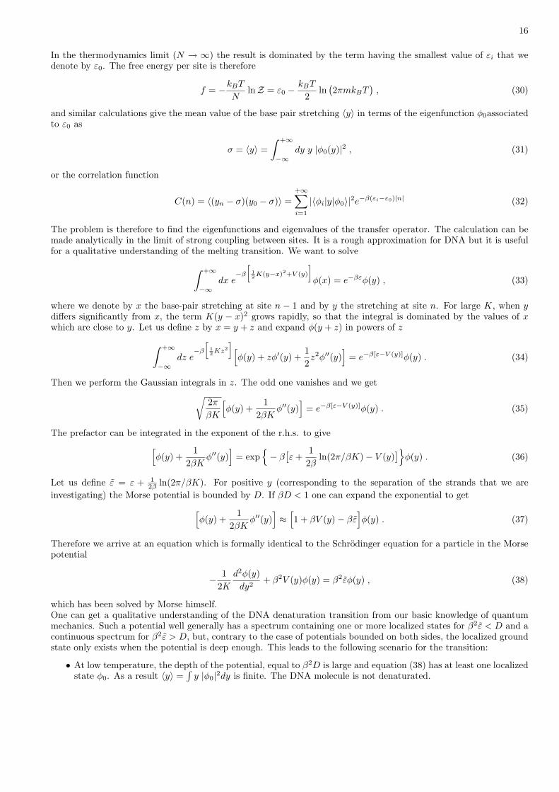
In the thermodynamics limit (N → ∞) the result is dominated by the term having the smallest value of εi that wedenote by ε0. The free energy per site is therefore

f = −kBT

NlnZ = ε0 − kBT

2ln

(2πmkBT

), (30)

and similar calculations give the mean value of the base pair stretching 〈y〉 in terms of the eigenfunction φ0associatedto ε0 as

σ = 〈y〉 =∫ +∞

−∞dy y |φ0(y)|2 , (31)

or the correlation function

C(n) = 〈(yn − σ)(y0 − σ)〉 =+∞∑

i=1

|〈φi|y|φ0〉|2e−β(εi−ε0)|n| (32)

The problem is therefore to find the eigenfunctions and eigenvalues of the transfer operator. The calculation can bemade analytically in the limit of strong coupling between sites. It is a rough approximation for DNA but it is usefulfor a qualitative understanding of the melting transition. We want to solve

∫ +∞

−∞dx e

−β

[12 K(y−x)2+V (y)

]φ(x) = e−βεφ(y) , (33)

where we denote by x the base-pair stretching at site n − 1 and by y the stretching at site n. For large K, when ydiffers significantly from x, the term K(y − x)2 grows rapidly, so that the integral is dominated by the values of xwhich are close to y. Let us define z by x = y + z and expand φ(y + z) in powers of z

∫ +∞

−∞dz e

−β

[12 Kz2

][φ(y) + zφ′(y) +

12z2φ′′(y)

]= e−β[ε−V (y)]φ(y) . (34)

Then we perform the Gaussian integrals in z. The odd one vanishes and we get√

2π

βK

[φ(y) +

12βK

φ′′(y)]

= e−β[ε−V (y)]φ(y) . (35)

The prefactor can be integrated in the exponent of the r.h.s. to give[φ(y) +

12βK

φ′′(y)]

= exp{− β

[ε +

12β

ln(2π/βK)− V (y)]}

φ(y) . (36)

Let us define ε = ε + 12β ln(2π/βK). For positive y (corresponding to the separation of the strands that we are

investigating) the Morse potential is bounded by D. If βD < 1 one can expand the exponential to get[φ(y) +

12βK

φ′′(y)]≈

[1 + βV (y)− βε

]φ(y) . (37)

Therefore we arrive at an equation which is formally identical to the Schrodinger equation for a particle in the Morsepotential

− 12K

d2φ(y)dy2

+ β2V (y)φ(y) = β2εφ(y) , (38)

which has been solved by Morse himself.One can get a qualitative understanding of the DNA denaturation transition from our basic knowledge of quantummechanics. Such a potential well generally has a spectrum containing one or more localized states for β2ε < D and acontinuous spectrum for β2ε > D, but, contrary to the case of potentials bounded on both sides, the localized groundstate only exists when the potential is deep enough. This leads to the following scenario for the transition:

• At low temperature, the depth of the potential, equal to β2D is large and equation (38) has at least one localizedstate φ0. As a result 〈y〉 =

∫y |φ0|2dy is finite. The DNA molecule is not denaturated.

17

• When temperature increases, the depth of the potential decreases and, for a critical temperature Tc the localizedstate merges into the continuum. The ground state is a non-localized eigenfunction of the continuum and 〈y〉diverges. DNA is denaturated.

This scenario is independent of the exact expression of the potential, provided it is qualitatively similar to the Morsepotential. This is an important feature because, as we have discussed above, the potential is not exactly known.For the Morse potential, the calculation shows that

Tc =2√

2KD

akB. (39)

B. Comparison with experiments: improving the model.

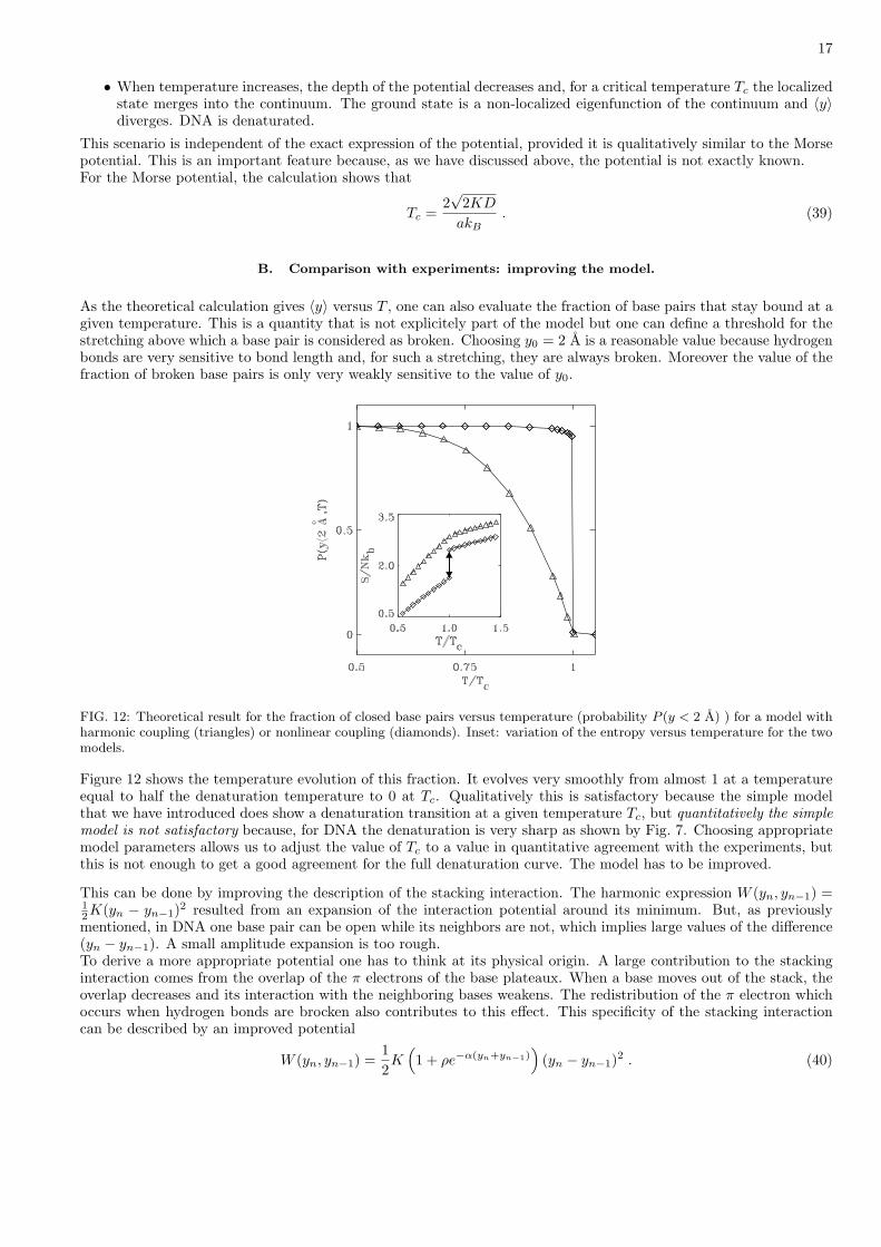
As the theoretical calculation gives 〈y〉 versus T , one can also evaluate the fraction of base pairs that stay bound at agiven temperature. This is a quantity that is not explicitely part of the model but one can define a threshold for thestretching above which a base pair is considered as broken. Choosing y0 = 2 A is a reasonable value because hydrogenbonds are very sensitive to bond length and, for such a stretching, they are always broken. Moreover the value of thefraction of broken base pairs is only very weakly sensitive to the value of y0.

FIG. 12: Theoretical result for the fraction of closed base pairs versus temperature (probability P (y < 2 A) ) for a model withharmonic coupling (triangles) or nonlinear coupling (diamonds). Inset: variation of the entropy versus temperature for the twomodels.

Figure 12 shows the temperature evolution of this fraction. It evolves very smoothly from almost 1 at a temperatureequal to half the denaturation temperature to 0 at Tc. Qualitatively this is satisfactory because the simple modelthat we have introduced does show a denaturation transition at a given temperature Tc, but quantitatively the simplemodel is not satisfactory because, for DNA the denaturation is very sharp as shown by Fig. 7. Choosing appropriatemodel parameters allows us to adjust the value of Tc to a value in quantitative agreement with the experiments, butthis is not enough to get a good agreement for the full denaturation curve. The model has to be improved.

This can be done by improving the description of the stacking interaction. The harmonic expression W (yn, yn−1) =12K(yn − yn−1)2 resulted from an expansion of the interaction potential around its minimum. But, as previouslymentioned, in DNA one base pair can be open while its neighbors are not, which implies large values of the difference(yn − yn−1). A small amplitude expansion is too rough.To derive a more appropriate potential one has to think at its physical origin. A large contribution to the stackinginteraction comes from the overlap of the π electrons of the base plateaux. When a base moves out of the stack, theoverlap decreases and its interaction with the neighboring bases weakens. The redistribution of the π electron whichoccurs when hydrogen bonds are brocken also contributes to this effect. This specificity of the stacking interactioncan be described by an improved potential

W (yn, yn−1) =12K

(1 + ρe−α(yn+yn−1)

)(yn − yn−1)2 . (40)

18

It is important to notice the plus sign in the exponential term, which is very important. As soon as either one of thetwo interacting base pairs is open (an not necessarily both simultaneously) the effective coupling constant drops fromK ′ ≈ K(1 + ρ) down to K ′ = K.

The calculations performed with the harmonic stacking interaction in order to reduce the determination of the eigen-functions of the transfer operator to a pseudo-Schrodinger equation are no longer valid because the coupling term isno longer a function of the difference (y − x). Equation (28) has to be solved numerically. Discretizing space, theproblem is turned into the diagonalization of a matrix. The accuracy of the calculation can be improved by usingintegration schemes such as Gauss-Hermite quadratures [32] and a finite scaling analysis [33] can be used to take careof the finiteness of the integration domain.Figure 12 shows that the nonlinear stacking interaction drastically modifies the character of the denaturation transitionof the model. It becomes very sharp, first-order like, in good agreement with the experimental observations [34]. Acareful study shows that the transition is not infinitely sharp (first order). It occurs smoothly but within a verynarrow temperature domain, the width of which is controlled by the value of the parameter α. The entropy almostshows a jump at the transition, as shown in Fig. 12, which corresponds to an effective latent heat. The role of thenonlinear stacking to modify the character of the transition can be understood from simple qualitative arguments.Above denaturation, the stacking gets weaker, reducing the rigidity of the DNA strands, i.e. increasing their entropy.Although there is a energetic cost to open the base pairs, if the entropy gain is large enough, the opening may thusbring a gain in free energy F = U−TS, where U is the internal energy of the system and S its entropy. The nonlinearstacking leads to a kind of “self-amplification process” in the transition: when the transition proceeds, the extraflexibility of the strands makes it easier, which sustains the denaturation that becomes very sharp.

C. Another view of the transition: stability of the thermalized domain wall.

We have seen that the equation of motion of the DNA model has a domain wall solution (22) which separates an openand a closed region. In the absence of thermal fluctuations the domain wall is unstable and it tends to move in thedirection that closes the open region to reduce its energy. Let us now investigate the properties of the domain wall inthe presence of thermal fluctuations and calculate its free energy.In order to analyze the fluctuations around the domain wall, let us look for a solution of Eq. (18) of the formY (x, t) = YDW (x) + f(x, t), where YDW (x) is the domain wall solution (22) centered at position x0, and assume thatf(x, t) is small enough, which allows us to linearize the equation in f . Putting Y (x, t) in Eq. (18) and linearizing inf , one gets

∂2f

∂t2− S

∂2f

∂x2+ V(x)f(x, t) = 0 , (41)

where

V(x) =(

∂2V [Y = YDW (x)]∂Y 2

)= −2

ez − 1(1 + ez)2

with z =

√2S

(x− x0) . (42)

If we look for a solution under the form f(x, t) = e−iωt g(x) we get for g(x) a Schrodinger-like equation

−S∂2g

dx2+ V(x) g(x) = ω2g(x) . (43)

The eigenvalues ω2 associated to the effective potential V(x) determine the spectrum of the small amplitude oscillationsaround the domain wall. Far from the center of the wall, the effective potential V(x) tends to 0 on the open side andto 2 on the closed side of the wall. It is such that it has no bound states, but we can predict the existence of twokinds of extended states:

• For ω2 < 2 the states will only extend in the region x > x0.

• For ω2 > 2 the states are extended on both sides of the wall, but the dispersion relation of the waves is differentfor x < x0 and x > x0.

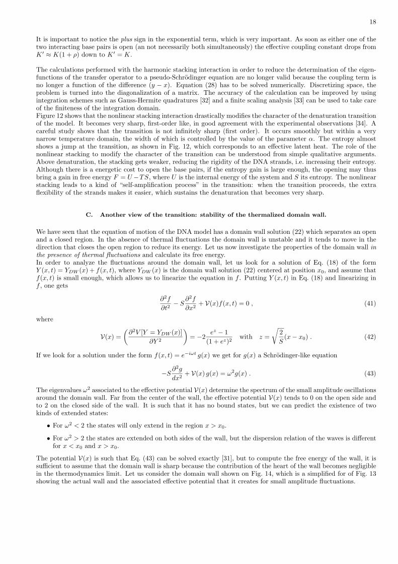
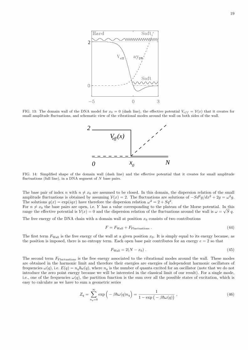
The potential V(x) is such that Eq. (43) can be solved exactly [31], but to compute the free energy of the wall, it issufficient to assume that the domain wall is sharp because the contribution of the heart of the wall becomes negligiblein the thermodynamics limit. Let us consider the domain wall shown on Fig. 14, which is a simplified for of Fig. 13showing the actual wall and the associated effective potential that it creates for small amplitude fluctuations.

19

2

FIG. 13: The domain wall of the DNA model for x0 = 0 (dash line), the effective potential Veff = V(x) that it creates forsmall amplitude fluctuations, and schematic view of the vibrational modes around the wall on both sides of the wall.

N

V (x)2

0 x

eff

0

FIG. 14: Simplified shape of the domain wall (dash line) and the effective potential that it creates for small amplitudefluctuations (full line), in a DNA segment of N base pairs.

The base pair of index n with n 6= x0 are assumed to be closed. In this domain, the dispersion relation of the smallamplitude fluctuations is obtained by assuming V(x) = 2. The fluctuations are solutions of −Sd2g/dx2 + 2g = ω2g.The solutions g(x) = exp(iqx) have therefore the dispersion relation ω2 = 2 + Sq2.For n 6= x0 the base pairs are open, i.e. Y has a value corresponding to the plateau of the Morse potential. In thisrange the effective potential is V(x) = 0 and the dispersion relation of the fluctuations around the wall is ω =

√S q.

The free energy of the DNA chain with a domain wall at position x0 consists of two contributions

F = FWall + FFluctuations . (44)

The first term FWall is the free energy of the wall at a given position x0. It is simply equal to its energy because, asthe position is imposed, there is no entropy term. Each open base pair contributes for an energy e = 2 so that

FWall = 2(N − x0) . (45)

The second term FFluctuations is the free energy associated to the vibrational modes around the wall. These modesare obtained in the harmonic limit and therefore their energies are energies of independent harmonic oscillators offrequencies ω(q), i.e. E(q) = nq~ω(q), where nq is the number of quanta excited for an oscillator (note that we do notintroduce the zero point energy because we will be interested in the classical limit of our result). For a single mode,i.e., one of the frequencies ω(q), the partition function is the sum over all the possible states of excitation, which iseasy to calculate as we have to sum a geometric series

Zq =∞∑

nq=0

exp(− β~ω(q)nq

)=

11− exp

(− β~ω(q)) , (46)

20

which gives the usual Bose-Einstein expression. In the classical limit ~ω(q) ¿ kBT one can replace the exponentialby its lowest order expansion exp(−β~ω(q)) ' 1− β~ω(q) so that one gets

Zq =1

β~ω(q). (47)

One can notice that, for the dynamics of DNA base pairs, the classical limit is perfectly justified. Typical oscillationfrequencies for the bases, which are big chemical groups, are 5 1011 Hz, giving ~ω ≈ 2 10−3 eV while kBT ≈ 0.025 eVat room temperature.The partition function of the set of independent modes, which gives the number of states of the set of modes, is theproduct of the partition functions for each mode

Z = Πq1

β~ω(q)(48)

giving the free energy of the fluctuations

Ffluctuations = −kBT ln Z = kBT∑

q

ln(β~ω(q)

). (49)

This discrete sum is not easy to calculate but we can replace it with an integral as the number of modes is very large.For a lattice of p particles, the possible wavevectors are qi = iπ/p (i = 0, . . . , p− 1 ), so that the variation of q for onemode to the next is ∆q = π/p, which gives a density of states 1/∆q = p/π. Using this density of states, one obtains

∑q

f [ω(q)] ' 1∆q

∫dq f [ω(q)] , (50)

where f [ω(q)] is an arbitrary function of ω(q).For a DNA molecule of N base pairs, having a domain wall at the base pair of index x0, we have x0 base pairs withthe dispersion relation ω(q) =

√2 + Sq2 and N − x0 pairs with the dispersion relation ω(q) =

√S q. Therefore one

gets

Ffluctuations = kBTx0

π

∫ ∞

0

dq ln β~√

2 + Sq2 + kBTN − x0

π

∫ ∞

0

dq ln β~√

S q , (51)

where the integrals over q have been extended to infinity, which is consistent with the continuum limit. Setting apartthe terms that depend on the position x0 of the wall, one gets

Ffluctuations =kBT

πx0

∫ ∞

0

dq ln

(√2 + Sq2

√S q

)+ F1 , (52)

where F1 is a quantity that does not depend on x0. The integral of Eq. (52), that we denote by I, can be calculatedusing

I =∫ ∞

0

dq ln√

2Sq2

+ 1 =12

∫ ∞

0

dq ln 1 +2

Sq2(53)

with the help of∫ ∞

0

duln(1 + u2)

u2= π , (54)

and setting u =√

2/S q. One gets

Ffluctuations = kBTx0

2

√2S

+ F1 . (55)

If one collects the results (45) and (55), one gets the following expression of the free energy of the DNA model witha domain wall at site x0

F = x0

[kBT

2

√2S− 2

]+ F ′1 , (56)

where F ′1 does not depend on x0.

21

• For small T (or for T = 0), the expression within the brackets is negative. The DNA segment car reduce its freeenergy by increasing x0, which tends to close the open base pairs, as we already noticed.

• On the contrary, for large T the term within the brackets becomes positive and the DNA segment can reduceits free energy by decreasing x0, i.e. by opening the base pairs that were closed.

• For (kBT/2)√

2/S = 2, i.e.

T = Tc =2

kB

√2S (57)

the free energy of the DNA segment is independent of the position of the domain wall. Therefore this temperatureappears as the transition temperature at which the molecule changes from the double helix to the denaturatedstate.

It is important to notice that, if one comes back to variables with dimensions by replacing S by its value S = K/(Da2),and taking into account that energies such as kBT must be multiplied by D to recover the true energy, one obtainsTc = 2

√2KD/(akB), which is exactly the denaturation temperature given by the Transfer Integral method (Eq. (39) ).

This calculation shows that, in addition to the standard approach to the denaturation transition, the calculation ofthe partition function using the Transfer Integral operator, one can also study the transition by investigating thefree energy of a nonlinear excitation, the domain wall. This method illustrates the interest of nonlinear science, andmoreover it turns out to be better than the conventional method because it provides an easy method to take intoaccount the effect of the discreteness of the lattice, which, for DNA are not negligible since S = 0.099 [31].

D. Discussion: Is a one-dimensional phase transition possible?

In statistical physics, it is often stated that there are no phase transitions in one dimensional systems with shortrange interactions. We have described above a simple system that does have such a phase transition. There isno contradiction because the “theorem” that forbids phase transitions in one-dimensional systems relies on somehypothesis:

• it is valid if the interactions are pair interactions, i.e. only depend on the difference of consecutive variables,such as (yn − yn−1). This is not true for the DNA model due to the term V (yn) coming from the interactionbetween the two strands of DNA. This term plays the same role as an external field on a magnetic system forinstance.

• it also requires that the domain walls between two regions have a finite energy. When this is the case, a simpleargument due to Landau can show that, for instance, a spin lattice is never in an ordered state. The reason isthat the cost of making a domain wall between a spin up region and a spin down one is finite and, contraryto higher dimensions, in one dimension it does not grow with the system size so that it becomes negligible inthe thermodynamic limit with respect to the total interaction energy in the system. Therefore the spin latticecan create many domains, increasing its entropy and breaking the order. This is no true for the DNA modelbecause, in the thermodynamic limit, i.e. for an infinite chain, the energy of a domain wall separating an openfrom a closed region is infinite.

VII. MODELING THE MECHANICAL DENATURATION OF DNA.

As mentioned in Sec. II B 2 it is now possible to manipulate single molecules of DNA. It is therefore tempting to tryto use this possibility to mechanically determine the sequence of DNA because a GC base pair, with three hydrogenbonds, is expected to be harder to break than an A − T base pair with only two bonds. Some experiments onthe micromechanical denaturation of DNA have been performed. Figure 15 shows a schematic view of the actualexperiment [35]. The DNA molecule to open is attached on one side to a DNA linker, itself attached to a glass plateproviding a fixed reference point. On the other hand, one of the strands is attached to a glass bead, which is pulledby a glass micro-needle. The necessary attachments are provided by the “biological glue” biotine–streptavidine, twomolecules that bind strongly to each other. It is possible to buy glass beads coated with spectravidine, and biologicaltechniques are used to chemically link biotine to the desired position of DNA. This experiments illustrates the powerof the combination of physical techniques to biological methods that can take advantage of the specificity of biological

22

���������

���������

Glass bead

DNA to open

DNA linker

Fixedattachement

moved atmicroneedle

constant speed

FIG. 15: Schematic picture of the micromechanical denaturation experiment of DNA.

reactions which are now well known and controlled, even if their mechanism is not yet fully understood at the molecularlevel. The micro-needle, moved at constant speed pulls the glass bead, leading to the mechanical denaturation of theDNA segment under study, but, in addition its elastic deformation which is recordered provides a measure of the forcewhich is necessary to break the base pairs.In fact a simple analysis shows that such an experiment is not able to distinguish a single base pair. The piece ofDNA strand which is already open and the needle are equivalent to an elastic spring of rigidity k1. When a basepair breaks, a length ∆` = 7.5 A is freed on each strand. As a result this spring shortens by 2∆` = 15 A. The forcethat it exerts on DNA decreases, but the decrease of the elastic energy stored in the spring is very small, well belowkBT and the denaturation does not stop immediately after the first mechanical denaturation has occurred. Assistedby thermal fluctuations, it goes on, along at least a few tens of base pairs, releasing the elastic stress sufficiently forthe elastic force to fall well below the critical force that denaturates a base pair. Therefore the experiment observesthe breaking of groups of base pairs and cannot be used for a mechanical sequencing of DNA. However, on a scale of100 bases the experiment shows a good correlation between the G − C content and the force necessary to open themolecule [35], showing that mechanical denaturation can give some information on the sequence at low resolution. Inorder to analyze this information it is however necessary to examine the results of the experiment in details becausethe relation between the measured force and the sequence is not trivial.

A. Numerical observation for a homopolymer.

The simplest case that one can consider is the case of an artificial DNA molecule having a single type of base pairs,such as the homopolymer that was used in some thermal denaturation experiments [14]. Actual single-moleculeexperiments on such systems have not yet been performed because it is hard to make long enough homopolymers. Letus examine the results of numerical simulations performed with the DNA model that we have introduced in Sec. III.

M

N

A

FB FA

�������������

�������������

C0

FIG. 16: Extension of the one-dimensional DNA model to describe micromechanical denaturation experiments. FA is the forcepulling the glass bead, i.e. the force measured by the experiment. FB is the force exerted by the strand which is alreadydenaturated at the level of base pair of index M , which is the next to break.

For such a study the model has to be slightly extended as shown on Fig. 16. As we have only one variable per basepair, the stretching of the bases, the overall translation of the base pairs is not considered and, instead of the linkerDNA, one can consider that one side of each base pair is attached to a fixed point. The elastic string, composed of thelinker DNA (which is very rigid and plays a little role, and the micro-needle, is represented by a spring of constant c0

which is attached to the base pair of index 1. One end of this spring (point A on the figure, whose position is denoted

23

by yA) is pulled at constant velocity v. The extension of the spring provides a measure of the force FA that pulls onthe DNA strand according to FA = c0(yA − y1), where yA = vt.The hamiltonian of this extended system is

HM =12c0(yA − y1)2+

p21

2m+ V (y1)

+N∑

n=2

12m

(dyn

dt

)2

+ W (yn, yn−1) + V (yn) ,

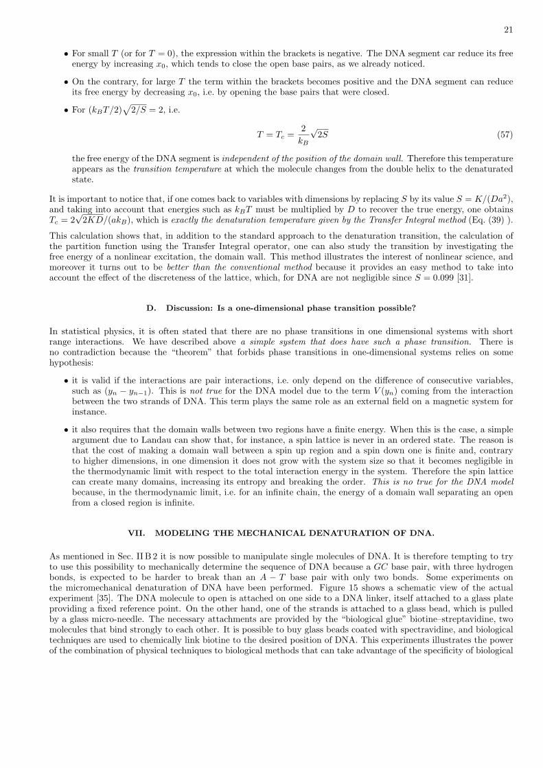
where, as before V is the on-site Morse potential and W the stacking interaction between the bases.Numerical simulations are performed at controlled temperature T using a chain of Nose thermostats coupled to thevariables y1 . . . yN but not to yA which is constrained (and in practice attached to a macroscopic object, the glassbead and the micro-needle, itself connected to a micromanipulator). Figure 17 shows typical results of a simulation.In the experiments the driving velocity is of 20 to 40 nm/s, i.e. 20 to 40 base pairs break per second. Even with a

(a) (b)

FIG. 17: Results of the numerical simulations of the mechanical denaturation of a DNA segment of 512 base pairs at T = 250 Kand a stretching velocity v = 0.0025 A/time unit. (a) Variation of the force FA (full line) and of the time derivative dM/dtof the number of broken base pairs (dash line). The unit of force in these simulations is 1 eV/A= 1.6 10−9 N = 1600 pN. (b)Stretching of the base pairs versus time on a scale ranging from white (fully closed) to back (fully open). The horizontal axisextends along the molecule and the vertical axis is the time axis.

simple model, simulations up to one second are not possible as they would require 1014 time steps. Simulations havebeen performed on time scales of the order of a ns, up to 0.5 µs for the longest. The driving speeds are therefore muchhigher than in the experiments as they are typically of 2 1011 nm/s, down to 108 nm/s for the longest simulation.This is considerably larger than in experiments, but the main point is that one must pull slowly enough to be in aregime where the speed does not affect the results. This is not true for velocities of 2 1011 nm/s because typical forcefor breaking are then approximately 64 pN, while they decrease to 16 pN for v = 108 nm/s. In this last case theforces no longer depend on v, so that one can consider that one can consider that v = 108 nm/s is low enough to getmeaningful results.The average breaking force obtained in the simulation is 16 pN, while experiments give about 13 pN. This provides anadditional test for the model parameters beyond the thermal denaturation, and confirm that they are correct because,which such a simple model, one cannot expect to reproduce experimental results with less than a 20% error.The main result is that, although we are working with a homopolymer, the breaking force shows very large oscillations,associated to the variation of the speed at which the breaking propagates. We have to understand this point, andthe theoretical analysis of the model will provide the clue. Moreover simulations show that the breaking does notoccur one base pair at a time. The propagation events involve 30 to 50 bases at once. This is in agreement with theexperiments and provides a further test of the validity of the model.

24

B. Analysis: kinetics of the denaturation.

1. Why does the molecule open?

Of course it is because we are pulling on it, but is it the only reason? The maximum of the slope of the Morsepotential, its slope at the inflexion point, gives the value of the maximum force that the potential can oppose tothe breaking force, Fmax = aD/2, which, with our model parameters is equal to 216 pN. Therefore the breaking isobserved for forces which are well below the strength of the Morse potential.Let us now consider the lifetime of a closed base pair. Simulations shows that 300 bases are broken in 2 105 t.u., i.e.approximately 660 t.u. are required to break a single base pair (and much more in actual experiments). This has tobe compared with the periods of oscillation at the bottom of the Morse potential tMorse = 2π/

√2Da2/m = 98.7 t.u.,

which shows that the base pairs can perform several oscillations (very many in the actual experiments) in the bottomof the Morse potential before the breaking.In the presence of a pulling force FB , the effective potential linking the bases becomes V ′(y) = V (y) − FB y. Fora force that exceeds the maximum strength that the Morse potential can sustain, V ′(y) would loose its minimum,leading to a pure mechanical breaking. For the forces used in the experiments and in the simulations, V ′(y) still has

1Y

FIG. 18: The effective potential acting on a base pair under the action of a pulling force.

a minimum separated from the dissociative state by a maximum for y = Y1 (Fig. 18). Therefore the stable state isthe unbroken base pair, and, if the breaking occurs, it is because it is thermally activated, i.e. it is assisted by thethermal fluctuations. Understanding the breaking amounts to understanding the escape from a potential well due tothermal fluctuations. This is a standard problem of chemical kinetics, similar to the dissociation of a molecule in ametastable state. It can be analyzed by the transition state theory.

2. Introduction to the transition state theory.

The theories of chemical reaction rates have looked at this problem from many view points. Simplest approachessay that molecular collisions are required to induce a reaction. Transition State Theory (TST) looks at the reactionpathway more completely [36]. The basic idea is that reactions may be represented by a particle motion in a potentialhypersurface in configuration space (Fig. 19). The dimension of this configuration space is the number of degrees offreedom in the system. Among all the degrees of freedom, one variable can be considered as representative of thechemical reaction (for instance the stretching of a bond that will dissociate). It is called the reaction coordinate. Inthis multidimensional space, the domain of reactants is the region where the parameters have values correspondingto the initial stage of the reaction. The domain of products is associated to the final state. These two regions aregenerally separated by a bottleneck in phase space, associated to a local maximum in energy. It is the transition state.The reaction is the evolution from the reactant domain to the product domain, through the transition state.

The basis assumptions of the transition state theory are the following:

(i) Thermal equilibrium: all states of the system, whether they are stable or metastable states, are treated as if thesystem was in equilibrium. Strictly speaking, this cannot be true because the system is undergoing a chemical

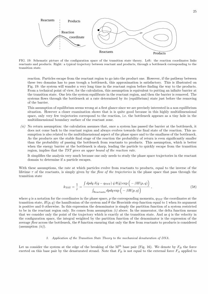
25

Reactants Products

Reactioncoordinate

Reactants Products

FIG. 19: Schematic picture of the configuration space of the transition state theory. Left: the reaction coordinates linksreactants and products. Right: a typical trajectory between reactant and products, through a bottleneck corresponding to thetransition state.

reaction. Particles escape from the reactant region to go into the product one. However, if the pathway betweenthese two domains has to pass trough a bottleneck, this approximation is satisfactory. This is illustrated onFig. 19: the system will wander a very long time in the reactant region before finding the way to the products.From a technical point of view, for the calculation, this assumption is equivalent to putting an infinite barrier atthe transition state. One lets the system equilibrate in the reactant region, and then the barrier is removed. Thesystems flows through the bottleneck at a rate determined by its (equilibrium) state just before the removingof the barrier.This assumption of equilibrium seems wrong at a first glance since we are precisely interested in a non equilibriumsituation. However a closer examination shows that is is quite good because in this highly multidimensionalspace, only very few trajectories correspond to the reaction, i.e. the bottleneck appears as a tiny hole in themultidimensional boundary surface of the reactant zone.

(ii) No return assumption: the calculation assumes that, once a system has passed the barrier at the bottleneck, itdoes not come back to the reactant region and always evolves towards the final state of the reaction. This as-sumption is also related to the multidimensional aspect of the phase space and to the smallness of the bottleneck.As the products are the stable final stage of the reaction the probability of return is even significantly smallerthan the probability of passing the bottleneck from reactants to products. This assumption, which is betterwhen the energy barrier at the bottleneck is sharp, leading the particle to quickly escape from the transitionregion, implies that the TST gives an upper bound of the reaction rate.It simplifies the analysis very much because one only needs to study the phase space trajectories in the reactantdomain to determine if a particle escapes.

With these assumptions, the rate at which particles evolve from reactants to products, equal to the inverse of thelifetime τ of the reactants, is simply given by the flow of the trajectories in the phase space that pass through thetransition state

kTST =1τ

=

∫dpdq δ(q − qTST) q θ(q) exp

(− βH(p, q)

)

∫Reactants

dpdq exp(− βH(p, q)

) , (58)

where q is a notation for the coordinates in the phase space, p the corresponding momenta, qTST the coordinates at thetransition state, H(p, q) the hamiltonian of the system and θ the Heaviside step function equal to 1 when its argumentis positive and 0 otherwise. In this expression the denominator is simply the partition function of a system restrictedto be in the reactant region only. Its comes from assumption (i) above. In the numerator, the delta function meansthat we consider only the point of the trajectory which is exactly at the transition state. And as q is the velocity inthe configuration space, the integral weighted by the partition function of the denominator is the expression of theaverage flow across the bottleneck, the θ function ensuring that only the flow from reactants to products is considered(assumption (ii)).

3. Application of the Transition State Theory to the mechanical denaturation of DNA.

Let us consider the system at the edge of the breaking of the Mth base pair (Fig. 16). We denote by FB the forceexerted on this base pair by the denaturated strand. Note that FB is not equal to the external force FA applied to

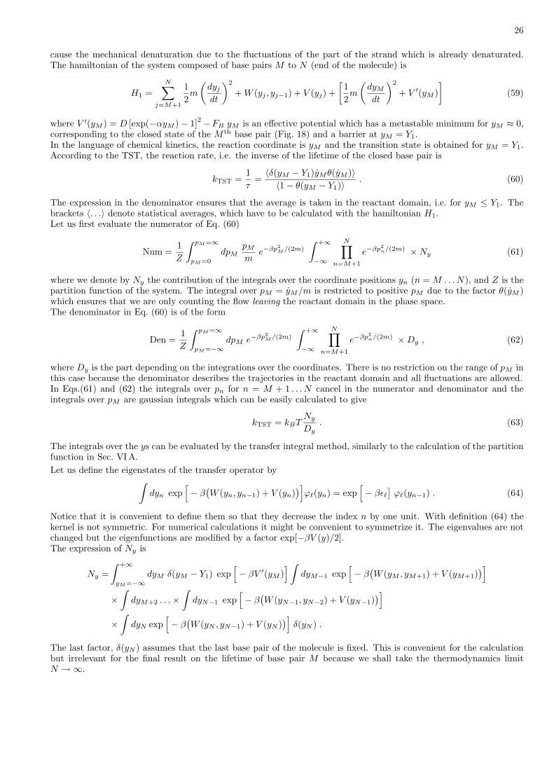
26

cause the mechanical denaturation due to the fluctuations of the part of the strand which is already denaturated.The hamiltonian of the system composed of base pairs M to N (end of the molecule) is

H1 =N∑

j=M+1

12m

(dyj

dt

)2

+ W (yj , yj−1) + V (yj) +[12m

(dyM

dt

)2

+ V ′(yM )]

(59)

where V ′(yM ) = D [exp(−αyM )− 1]2−FB yM is an effective potential which has a metastable minimum for yM ≈ 0,corresponding to the closed state of the M th base pair (Fig. 18) and a barrier at yM = Y1.In the language of chemical kinetics, the reaction coordinate is yM and the transition state is obtained for yM = Y1.According to the TST, the reaction rate, i.e. the inverse of the lifetime of the closed base pair is

kTST =1τ

=〈δ(yM − Y1)yMθ(yM )〉〈1− θ(yM − Y1)〉 . (60)

The expression in the denominator ensures that the average is taken in the reactant domain, i.e. for yM ≤ Y1. Thebrackets 〈. . .〉 denote statistical averages, which have to be calculated with the hamiltonian H1.Let us first evaluate the numerator of Eq. (60)

Num =1Z

∫ pM=∞

pM=0

dpMpM

me−βp2

M /(2m)

∫ +∞

−∞

N∏

n=M+1

e−βp2n/(2m) ×Ny (61)

where we denote by Ny the contribution of the integrals over the coordinate positions yn (n = M . . . N), and Z is thepartition function of the system. The integral over pM = yM/m is restricted to positive pM due to the factor θ(yM )which ensures that we are only counting the flow leaving the reactant domain in the phase space.The denominator in Eq. (60) is of the form

Den =1Z

∫ pM=∞

pM=−∞dpM e−βp2

M /(2m)

∫ +∞

−∞

N∏

n=M+1

e−βp2n/(2m) ×Dy , (62)

where Dy is the part depending on the integrations over the coordinates. There is no restriction on the range of pM inthis case because the denominator describes the trajectories in the reactant domain and all fluctuations are allowed.In Eqs.(61) and (62) the integrals over pn for n = M + 1 . . . N cancel in the numerator and denominator and theintegrals over pM are gaussian integrals which can be easily calculated to give

kTST = kBTNy

Dy. (63)

The integrals over the ys can be evaluated by the transfer integral method, similarly to the calculation of the partitionfunction in Sec. VI A.Let us define the eigenstates of the transfer operator by

∫dyn exp

[− β

(W (yn, yn−1) + V (yn)

)]ϕ`(yn) = exp

[− βε`

]ϕ`(yn−1) . (64)

Notice that it is convenient to define them so that they decrease the index n by one unit. With definition (64) thekernel is not symmetric. For numerical calculations it might be convenient to symmetrize it. The eigenvalues are notchanged but the eigenfunctions are modified by a factor exp[−βV (y)/2].The expression of Ny is

Ny =∫ +∞

yM=−∞dyM δ(yM − Y1) exp

[− βV ′(yM )

] ∫dyM−1 exp

[− β

(W (yM , yM+1) + V (yM+1)

)]

×∫

dyM+2 . . .×∫

dyN−1 exp[− β

(W (yN−1, yN−2) + V (yN−1)

)]

×∫

dyN exp[− β

(W (yN , yN−1) + V (yN )

)]δ(yN ) .

The last factor, δ(yN ) assumes that the last base pair of the molecule is fixed. This is convenient for the calculationbut irrelevant for the final result on the lifetime of base pair M because we shall take the thermodynamics limitN →∞.

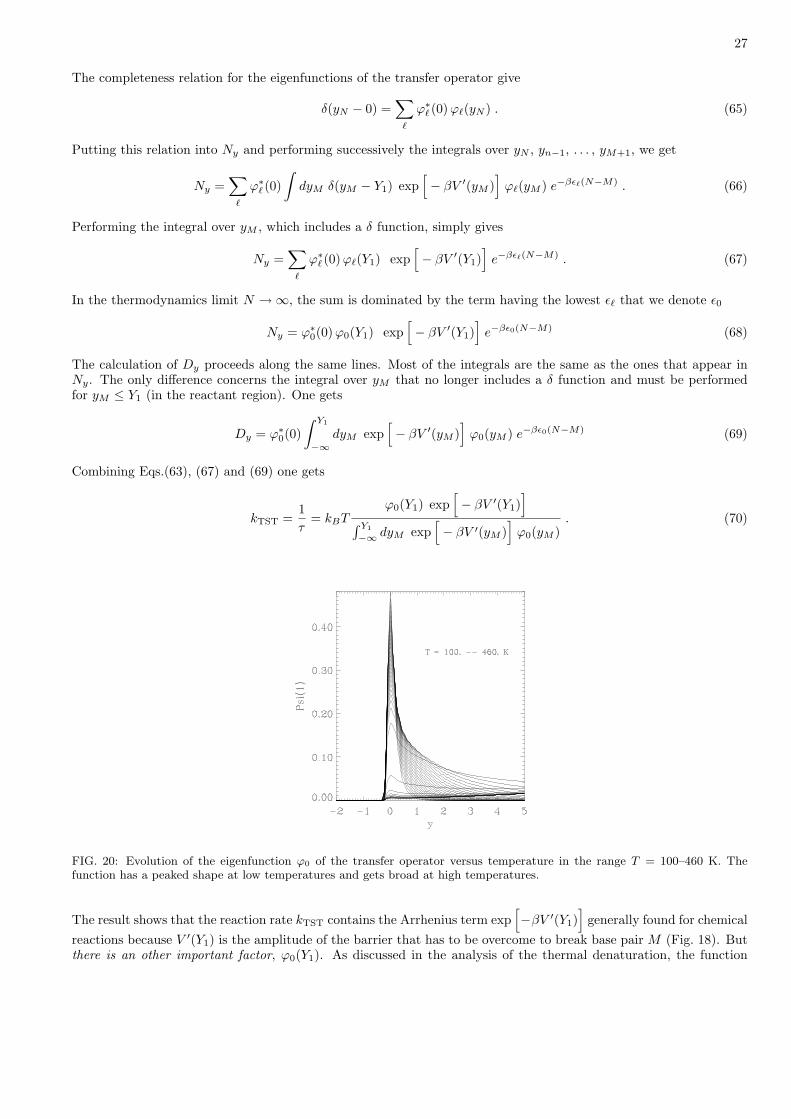
27

The completeness relation for the eigenfunctions of the transfer operator give

δ(yN − 0) =∑

`

ϕ∗` (0)ϕ`(yN ) . (65)

Putting this relation into Ny and performing successively the integrals over yN , yn−1, . . . , yM+1, we get

Ny =∑

`

ϕ∗` (0)∫

dyM δ(yM − Y1) exp[− βV ′(yM )

]ϕ`(yM ) e−βε`(N−M) . (66)

Performing the integral over yM , which includes a δ function, simply gives

Ny =∑

`

ϕ∗` (0) ϕ`(Y1) exp[− βV ′(Y1)

]e−βε`(N−M) . (67)

In the thermodynamics limit N →∞, the sum is dominated by the term having the lowest ε` that we denote ε0

Ny = ϕ∗0(0) ϕ0(Y1) exp[− βV ′(Y1)

]e−βε0(N−M) (68)

The calculation of Dy proceeds along the same lines. Most of the integrals are the same as the ones that appear inNy. The only difference concerns the integral over yM that no longer includes a δ function and must be performedfor yM ≤ Y1 (in the reactant region). One gets

Dy = ϕ∗0(0)∫ Y1

−∞dyM exp

[− βV ′(yM )

]ϕ0(yM ) e−βε0(N−M) (69)

Combining Eqs.(63), (67) and (69) one gets

kTST =1τ

= kBTϕ0(Y1) exp

[− βV ′(Y1)

]

∫ Y1

−∞ dyM exp[− βV ′(yM )

]ϕ0(yM )

. (70)

FIG. 20: Evolution of the eigenfunction ϕ0 of the transfer operator versus temperature in the range T = 100–460 K. Thefunction has a peaked shape at low temperatures and gets broad at high temperatures.

The result shows that the reaction rate kTST contains the Arrhenius term exp[−βV ′(Y1)

]generally found for chemical

reactions because V ′(Y1) is the amplitude of the barrier that has to be overcome to break base pair M (Fig. 18). Butthere is an other important factor, ϕ0(Y1). As discussed in the analysis of the thermal denaturation, the function

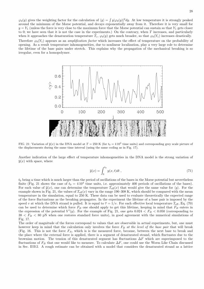
28

ϕ0(y) gives the weighting factor for the calculation of 〈y〉 =∫

y|ϕ0(y)|2dy. At low temperature it is strongly peakedaround the minimum of the Morse potential, and decays exponentially away from it. Therefore it is very small fory = Y1 (unless the force is very close to the maximum force that the Morse potential can sustain so that Y1 gets closerto 0; we have seen that it is not the case in the experiments.) On the contrary, when T increases, and particularlywhen it approaches the denaturation temperature Tc, ϕ0(y) gets much broader, so that ϕ0(Y1) increases drastically.Therefore ϕ0(Y1) appears as an amplification factor which increases the effect of temperature on the probability ofopening. As a result temperature inhomogeneities, due to nonlinear localization, play a very large role to determinethe lifetime of the base pairs under stretch. This explains why the propagation of the mechanical breaking is soirregular, even for a homopolymer.

FIG. 21: Variation of y(x) in the DNA model at T = 250 K (for t0 = 4104 time units) and corresponding grey scale picture ofthe displacements during the same time interval (using the same coding as in Fig. 17).

Another indication of the large effect of temperature inhomogeneities in the DNA model is the strong variation ofy(x) with space, where

y(x) =∫ t0

0

y(x, t)dt , (71)

t0 being a time which is much larger than the period of oscillations of the bases in the Morse potential but neverthelessfinite (Fig. 21 shows the case of t0 = 4 104 time units, i.e. approximately 400 periods of oscillations of the bases).For each value of y(x), one can determine the temperature Teff(x) that would give the same value for 〈y〉. For theexample shown in Fig. 21, the values of Teff(x) vary in the range 190–308 K, which should be compared with the meantemperature in the simulation, equal to 250 K. These data can be used to evaluate theoretically the expected rangeof the force fluctuations as the breaking propagates. In the experiment the lifetime of a base pair is imposed by thespeed v at which the DNA strand is pulled. It is equal to τ = 1/v. For each effective local temperature Teff , Eq. (70)can be used to determine which force FB one should apply to get this lifetime, keeping in mind that FB enters inthe expression of the potential V ′(y). For the example of Fig. 21, one gets 0.024 < FB < 0.050 (corresponding to38 < FB < 80 pN when one restores standard force units), in good agreement with the numerical simulations ofFig. 17.The order of magnitude of the forces correspond to values that are observable in actual experiments, but, one musthowever keep in mind that the calculation only involves the force FB at the level of the base pair that will break(Fig. 16. This is not the force FA, which is is the measured force, because, between the next base to break andthe place where the external force is applied, there is a segment of denaturated strand, which fluctuates due to thebrownian motion. The tension of this denaturated segment has fluctuations ∆F which are superimposed to thefluctuations of FB that one would like to measure. To calculate ∆F , one could use the Worm Like Chain discussedin Sec. II B 2. A rough estimate can be obtained with a model that considers the denaturated strand as a lattice

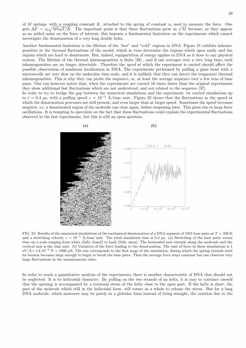
29

of M springs, with a coupling constant K, attached to the spring of constant c0 used to measure the force. Onegets ∆F = c0

√MkBT/K. The important point is that these fluctuations grow as

√M because, as they appear

as an added noise on the force of interest, this imposes a fundamental limitation on the experiments which cannotinvestigate the denaturation of a very long double helix.

Another fundamental limitation is the lifetime of the “hot” and “cold” regions in DNA. Figure 21 exhibits inhomo-geneities in the thermal fluctuations of the model, which in turn determine the regions which open easily and theregions which are hard to denaturate. But, indeed, equipartition of energy applies to DNA as it does to any physicalsystem. The lifetime of the thermal inhomogeneities is finite [38] , and if one averages over a very long time, suchinhomogeneities are no longer detectable. Therefore the speed at which the experiment is carried should affect thepossible observation of nonlinear localization in DNA. The experiments performed by pulling a glass bead with amicroneedle are very slow on the molecular time scale, and it is unlikely that they can detect the temporary thermalinhomogeneities. This is why they can probe the sequence, or, at least the average sequence over a few tens of basepairs. One can however notice that, when the experiments are carried 10 times faster than the original experimentsthey show additional fast fluctuations which are not understood, and not related to the sequence [37].In order to try to bridge the gap between the numerical simulations and the experiment, we carried simulations upto t = 0.4 µs, with a pulling speed v = 10−5 A/time unit. Figure 22 shows that the fluctuations in the speed atwhich the denaturation processes are still present, and even larger than at larger speed. Sometimes the speed becomesnegative, i.e. a denaturated region of the molecule can close again, before reopening later. This gives rise to large forceoscillations. It is tempting to speculate on the fact that these fluctuations could explain the experimental fluctuationsobserved in the fast experiments, but this is still an open question.

(a) (b)

FIG. 22: Results of the numerical simulations of the mechanical denaturation of a DNA segment of 1024 base pairs at T = 320 Kand a stretching velocity v = 10−5 A/time unit. The total simulation time is 0.4 µs. (a) Stretching of the base pairs versustime on a scale ranging from white (fully closed) to back (fully open). The horizontal axis extends along the molecule and thevertical axis is the time axis. (b) Variation of the force leading to the denaturation. The unit of force in these simulations is 1eV/A= 1.6 10−9 N = 1600 pN. The rise corresponds to the first stage of the simulation, during which the spring extends untilits tension becomes large enough to begin to break the base pairs. Then the average force stays constant but one observes verylarge fluctuations in the instantaneous value.

In order to reach a quantitative analysis of the experiments, there is another characteristic of DNA that should notbe neglected. It is its helicoidal character. By pulling on the two strands of an helix, it is easy to convince oneselfthat the opening is accompanied by a torsional stress of the helix close to the open part. If the helix is short, thepart of the molecule which still in the helicoidal form, will rotate as a whole to release the stress. But for a longDNA molecule, which moreover may be partly in a globular form instead of being straight, the rotation due to the

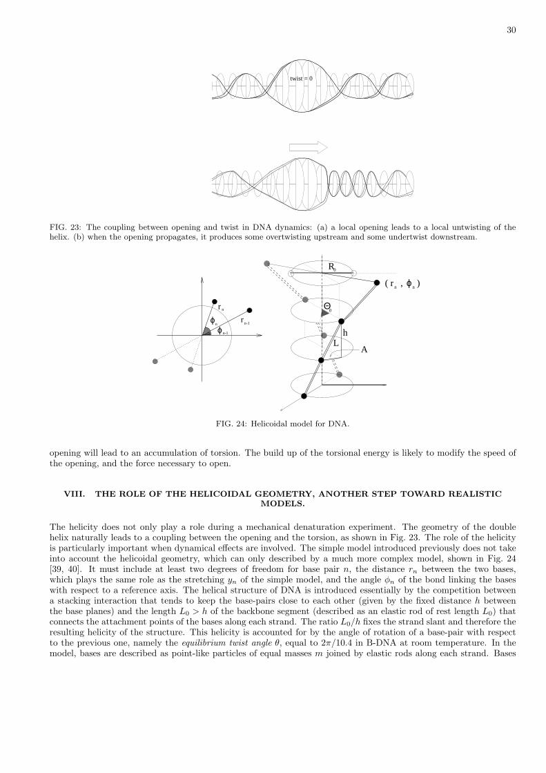
30

(b)

localtwist

(a)

twist = 0

FIG. 23: The coupling between opening and twist in DNA dynamics: (a) a local opening leads to a local untwisting of thehelix. (b) when the opening propagates, it produces some overtwisting upstream and some undertwist downstream.

ϕϕ

n

n-1

r

r

n-1

n

0

h

A

R

Θ0

L

nϕn( r , )

FIG. 24: Helicoidal model for DNA.

opening will lead to an accumulation of torsion. The build up of the torsional energy is likely to modify the speed ofthe opening, and the force necessary to open.

VIII. THE ROLE OF THE HELICOIDAL GEOMETRY, ANOTHER STEP TOWARD REALISTICMODELS.

The helicity does not only play a role during a mechanical denaturation experiment. The geometry of the doublehelix naturally leads to a coupling between the opening and the torsion, as shown in Fig. 23. The role of the helicityis particularly important when dynamical effects are involved. The simple model introduced previously does not takeinto account the helicoidal geometry, which can only described by a much more complex model, shown in Fig. 24[39, 40]. It must include at least two degrees of freedom for base pair n, the distance rn between the two bases,which plays the same role as the stretching yn of the simple model, and the angle φn of the bond linking the baseswith respect to a reference axis. The helical structure of DNA is introduced essentially by the competition betweena stacking interaction that tends to keep the base-pairs close to each other (given by the fixed distance h betweenthe base planes) and the length L0 > h of the backbone segment (described as an elastic rod of rest length L0) thatconnects the attachment points of the bases along each strand. The ratio L0/h fixes the strand slant and therefore theresulting helicity of the structure. This helicity is accounted for by the angle of rotation of a base-pair with respectto the previous one, namely the equilibrium twist angle θ, equal to 2π/10.4 in B-DNA at room temperature. In themodel, bases are described as point-like particles of equal masses m joined by elastic rods along each strand. Bases

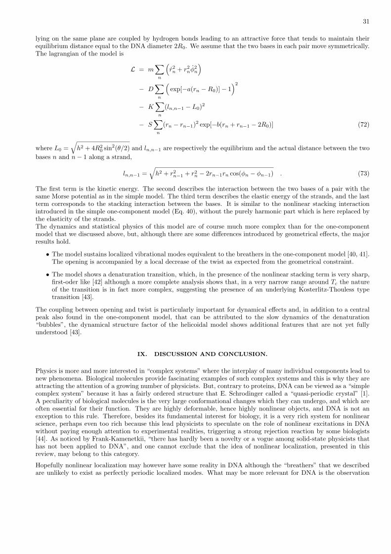
31

lying on the same plane are coupled by hydrogen bonds leading to an attractive force that tends to maintain theirequilibrium distance equal to the DNA diameter 2R0. We assume that the two bases in each pair move symmetrically.The lagrangian of the model is

L = m∑

n

(r2n + r2

nφ2n

)

− D∑

n

(exp[−a(rn −R0)]− 1

)2

− K∑

n

(ln,n−1 − L0)2

− S∑

n

(rn − rn−1)2 exp[−b(rn + rn−1 − 2R0)] (72)

where L0 =√

h2 + 4R20 sin2(θ/2) and ln,n−1 are respectively the equilibrium and the actual distance between the two

bases n and n− 1 along a strand,

ln,n−1 =√

h2 + r2n−1 + r2

n − 2rn−1rn cos(φn − φn−1) . (73)

The first term is the kinetic energy. The second describes the interaction between the two bases of a pair with thesame Morse potential as in the simple model. The third term describes the elastic energy of the strands, and the lastterm corresponds to the stacking interaction between the bases. It is similar to the nonlinear stacking interactionintroduced in the simple one-component model (Eq. 40), without the purely harmonic part which is here replaced bythe elasticity of the strands.The dynamics and statistical physics of this model are of course much more complex than for the one-componentmodel that we discussed above, but, although there are some differences introduced by geometrical effects, the majorresults hold.

• The model sustains localized vibrational modes equivalent to the breathers in the one-component model [40, 41].The opening is accompanied by a local decrease of the twist as expected from the geometrical constraint.

• The model shows a denaturation transition, which, in the presence of the nonlinear stacking term is very sharp,first-oder like [42] although a more complete analysis shows that, in a very narrow range around Tc the natureof the transition is in fact more complex, suggesting the presence of an underlying Kosterlitz-Thouless typetransition [43].

The coupling between opening and twist is particularly important for dynamical effects and, in addition to a centralpeak also found in the one-component model, that can be attributed to the slow dynamics of the denaturation“bubbles”, the dynamical structure factor of the helicoidal model shows additional features that are not yet fullyunderstood [43].

IX. DISCUSSION AND CONCLUSION.

Physics is more and more interested in “complex systems” where the interplay of many individual components lead tonew phenomena. Biological molecules provide fascinating examples of such complex systems and this is why they areattracting the attention of a growing number of physicists. But, contrary to proteins, DNA can be viewed as a “simplecomplex system” because it has a fairly ordered structure that E. Schrodinger called a “quasi-periodic crystal” [1].A peculiarity of biological molecules is the very large conformational changes which they can undergo, and which areoften essential for their function. They are highly deformable, hence highly nonlinear objects, and DNA is not anexception to this rule. Therefore, besides its fundamental interest for biology, it is a very rich system for nonlinearscience, perhaps even too rich because this lead physicists to speculate on the role of nonlinear excitations in DNAwithout paying enough attention to experimental realities, triggering a strong rejection reaction by some biologists[44]. As noticed by Frank-Kamenetkii, “there has hardly been a novelty or a vogue among solid-state physicists thathas not been applied to DNA”, and one cannot exclude that the idea of nonlinear localization, presented in thisreview, may belong to this category.

Hopefully nonlinear localization may however have some reality in DNA although the “breathers” that we describedare unlikely to exist as perfectly periodic localized modes. What may be more relevant for DNA is the observation

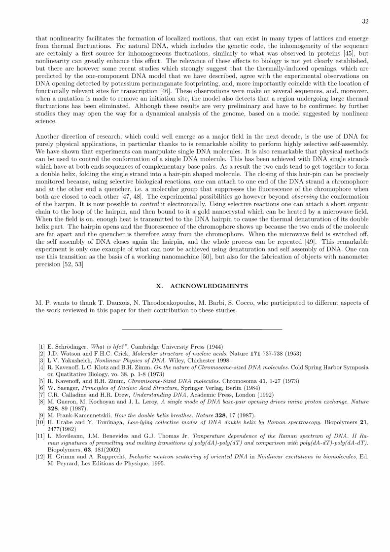
32

that nonlinearity facilitates the formation of localized motions, that can exist in many types of lattices and emergefrom thermal fluctuations. For natural DNA, which includes the genetic code, the inhomogeneity of the sequenceare certainly a first source for inhomogeneous fluctuations, similarly to what was observed in proteins [45], butnonlinearity can greatly enhance this effect. The relevance of these effects to biology is not yet clearly established,but there are however some recent studies which strongly suggest that the thermally-induced openings, which arepredicted by the one-component DNA model that we have described, agree with the experimental observations onDNA opening detected by potassium permanganate footprinting, and, more importantly coincide with the location offunctionally relevant sites for transcription [46]. These observations were make on several sequences, and, moreover,when a mutation is made to remove an initiation site, the model also detects that a region undergoing large thermalfluctuations has been eliminated. Although these results are very preliminary and have to be confirmed by furtherstudies they may open the way for a dynamical analysis of the genome, based on a model suggested by nonlinearscience.

Another direction of research, which could well emerge as a major field in the next decade, is the use of DNA forpurely physical applications, in particular thanks to is remarkable ability to perform highly selective self-assembly.We have shown that experiments can manipulate single DNA molecules. It is also remarkable that physical methodscan be used to control the conformation of a single DNA molecule. This has been achieved with DNA single strandswhich have at both ends sequences of complementary base pairs. As a result the two ends tend to get together to forma double helix, folding the single strand into a hair-pin shaped molecule. The closing of this hair-pin can be preciselymonitored because, using selective biological reactions, one can attach to one end of the DNA strand a chromophoreand at the other end a quencher, i.e. a molecular group that suppresses the fluorescence of the chromophore whenboth are closed to each other [47, 48]. The experimental possibilities go however beyond observing the conformationof the hairpin. It is now possible to control it electronically. Using selective reactions one can attach a short organicchain to the loop of the hairpin, and then bound to it a gold nanocrystal which can be heated by a microwave field.When the field is on, enough heat is transmitted to the DNA hairpin to cause the thermal denaturation of its doublehelix part. The hairpin opens and the fluorescence of the chromophore shows up because the two ends of the moleculeare far apart and the quencher is therefore away from the chromophore. When the microwave field is switched off,the self assembly of DNA closes again the hairpin, and the whole process can be repeated [49]. This remarkableexperiment is only one example of what can now be achieved using denaturation and self assembly of DNA. One canuse this transition as the basis of a working nanomachine [50], but also for the fabrication of objects with nanometerprecision [52, 53]

X. ACKNOWLEDGMENTS

M. P. wants to thank T. Dauxois, N. Theodorakopoulos, M. Barbi, S. Cocco, who participated to different aspects ofthe work reviewed in this paper for their contribution to these studies.

[1] E. Schrodinger, What is life?”, Cambridge University Press (1944)[2] J.D. Watson and F.H.C. Crick, Molecular structure of nucleic acids. Nature 171 737-738 (1953)[3] L.V. Yakusheich, Nonlinear Physics of DNA. Wiley, Chichester 1998.[4] R. Kavenoff, L.C. Klotz and B.H. Zimm, On the nature of Chromosome-sized DNA molecules. Cold Spring Harbor Symposia

on Quatitative Biology, vo. 38, p. 1-8 (1973)[5] R. Kavenoff, and B.H. Zimm, Chromisome-Sized DNA molecules. Chromosoma 41, 1-27 (1973)[6] W. Saenger, Principles of Nucleic Acid Structure, Springer Verlag, Berlin (1984)[7] C.R. Calladine and H.R. Drew, Understanding DNA, Academic Press, London (1992)[8] M. Gueron, M. Kochoyan and J. L. Leroy, A single mode of DNA base-pair opening drives imino proton exchange. Nature

328, 89 (1987).[9] M. Frank-Kamennetskii, How the double helix breathes. Nature 328, 17 (1987).

[10] H. Urabe and Y. Tominaga, Low-lying collective modes of DNA double helix by Raman spectroscopy. Biopolymers 21,2477(1982)

[11] L. Movileanu, J.M. Benevides and G.J. Thomas Jr, Temperature dependence of the Raman spectrum of DNA. II Ra-man signatures of premelting and melting transitions of poly(dA)-poly(dT) and comparison with poly(dA-dT)-poly(dA-dT).Biopolymers, 63, 181(2002)

[12] H. Grimm and A. Rupprecht, Inelastic neutron scattering of oriented DNA in Nonlinear excitations in biomolecules, Ed.M. Peyrard, Les Editions de Physique, 1995.

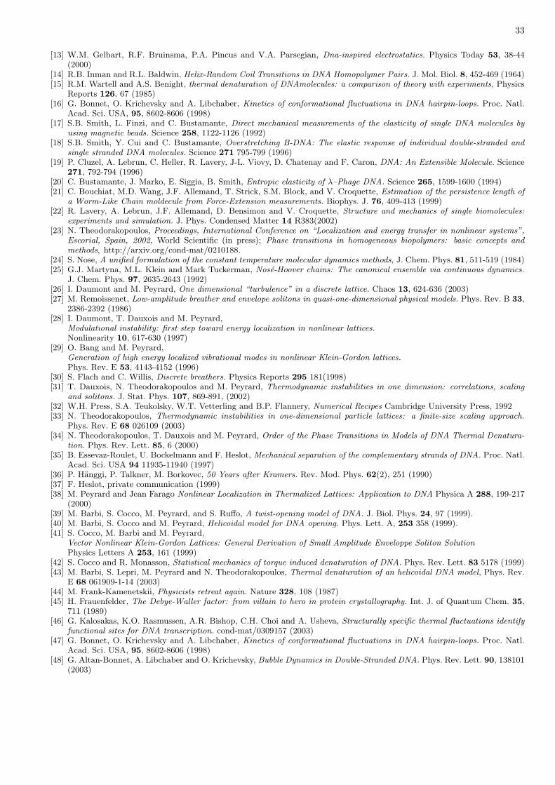
33

[13] W.M. Gelbart, R.F. Bruinsma, P.A. Pincus and V.A. Parsegian, Dna-inspired electrostatics. Physics Today 53, 38-44(2000)

[14] R.B. Inman and R.L. Baldwin, Helix-Random Coil Transitions in DNA Homopolymer Pairs. J. Mol. Biol. 8, 452-469 (1964)[15] R.M. Wartell and A.S. Benight, thermal denaturation of DNAmolecules: a comparison of theory with experiments, Physics

Reports 126, 67 (1985)[16] G. Bonnet, O. Krichevsky and A. Libchaber, Kinetics of conformational fluctuations in DNA hairpin-loops. Proc. Natl.

Acad. Sci. USA, 95, 8602-8606 (1998)[17] S.B. Smith, L. Finzi, and C. Bustamante, Direct mechanical measurements of the elasticity of single DNA molecules by

using magnetic beads. Science 258, 1122-1126 (1992)[18] S.B. Smith, Y. Cui and C. Bustamante, Overstretching B-DNA: The elastic response of individual double-stranded and

single stranded DNA molecules. Science 271 795-799 (1996)[19] P. Cluzel, A. Lebrun, C. Heller, R. Lavery, J-L. Viovy, D. Chatenay and F. Caron, DNA: An Extensible Molecule. Science

271, 792-794 (1996)[20] C. Bustamante, J. Marko, E. Siggia, B. Smith, Entropic elasticity of λ–Phage DNA. Science 265, 1599-1600 (1994)[21] C. Bouchiat, M.D. Wang, J.F. Allemand, T. Strick, S.M. Block, and V. Croquette, Estimation of the persistence length of

a Worm-Like Chain moldecule from Force-Extension measurements. Biophys. J. 76, 409-413 (1999)[22] R. Lavery, A. Lebrun, J.F. Allemand, D. Bensimon and V. Croquette, Structure and mechanics of single biomolecules:

experiments and simulation. J. Phys. Condensed Matter 14 R383(2002)[23] N. Theodorakopoulos, Proceedings, International Conference on “Localization and energy transfer in nonlinear systems”,

Escorial, Spain, 2002, World Scientific (in press); Phase transitions in homogeneous biopolymers: basic concepts andmethods, http://arxiv.org/cond-mat/0210188.

[24] S. Nose, A unified formulation of the constant temperature molecular dynamics methods, J. Chem. Phys. 81, 511-519 (1984)[25] G.J. Martyna, M.L. Klein and Mark Tuckerman, Nose-Hoover chains: The canonical ensemble via continuous dynamics.

J. Chem. Phys. 97, 2635-2643 (1992)[26] I. Daumont and M. Peyrard, One dimensional “turbulence” in a discrete lattice. Chaos 13, 624-636 (2003)[27] M. Remoissenet, Low-amplitude breather and envelope solitons in quasi-one-dimensional physical models. Phys. Rev. B 33,

2386-2392 (1986)[28] I. Daumont, T. Dauxois and M. Peyrard,

Modulational instability: first step toward energy localization in nonlinear lattices.Nonlinearity 10, 617-630 (1997)

[29] O. Bang and M. Peyrard,Generation of high energy localized vibrational modes in nonlinear Klein-Gordon lattices.Phys. Rev. E 53, 4143-4152 (1996)

[30] S. Flach and C. Willis, Discrete breathers. Physics Reports 295 181(1998)[31] T. Dauxois, N. Theodorakopoulos and M. Peyrard, Thermodynamic instabilities in one dimension: correlations, scaling

and solitons. J. Stat. Phys. 107, 869-891, (2002)[32] W.H. Press, S.A. Teukolsky, W.T. Vetterling and B.P. Flannery, Numerical Recipes Cambridge University Press, 1992[33] N. Theodorakopoulos, Thermodynamic instabilities in one-dimensional particle lattices: a finite-size scaling approach.

Phys. Rev. E 68 026109 (2003)[34] N. Theodorakopoulos, T. Dauxois and M. Peyrard, Order of the Phase Transitions in Models of DNA Thermal Denatura-

tion. Phys. Rev. Lett. 85, 6 (2000)[35] B. Essevaz-Roulet, U. Bockelmann and F. Heslot, Mechanical separation of the complementary strands of DNA. Proc. Natl.

Acad. Sci. USA 94 11935-11940 (1997)[36] P. Hanggi, P. Talkner, M. Borkovec, 50 Years after Kramers. Rev. Mod. Phys. 62(2), 251 (1990)[37] F. Heslot, private communication (1999)[38] M. Peyrard and Jean Farago Nonlinear Localization in Thermalized Lattices: Application to DNA Physica A 288, 199-217

(2000)[39] M. Barbi, S. Cocco, M. Peyrard, and S. Ruffo, A twist-opening model of DNA. J. Biol. Phys. 24, 97 (1999).[40] M. Barbi, S. Cocco and M. Peyrard, Helicoidal model for DNA opening. Phys. Lett. A, 253 358 (1999).[41] S. Cocco, M. Barbi and M. Peyrard,

Vector Nonlinear Klein-Gordon Lattices: General Derivation of Small Amplitude Enveloppe Soliton SolutionPhysics Letters A 253, 161 (1999)

[42] S. Cocco and R. Monasson, Statistical mechanics of torque induced denaturation of DNA. Phys. Rev. Lett. 83 5178 (1999)[43] M. Barbi, S. Lepri, M. Peyrard and N. Theodorakopoulos, Thermal denaturation of an helicoidal DNA model, Phys. Rev.

E 68 061909-1-14 (2003)[44] M. Frank-Kamenetskii, Physicists retreat again. Nature 328, 108 (1987)[45] H. Frauenfelder, The Debye-Waller factor: from villain to hero in protein crystallography. Int. J. of Quantum Chem. 35,

711 (1989)[46] G. Kalosakas, K.O. Rasmussen, A.R. Bishop, C.H. Choi and A. Usheva, Structurally specific thermal fluctuations identify

functional sites for DNA transcription. cond-mat/0309157 (2003)[47] G. Bonnet, O. Krichevsky and A. Libchaber, Kinetics of conformational fluctuations in DNA hairpin-loops. Proc. Natl.

Acad. Sci. USA, 95, 8602-8606 (1998)[48] G. Altan-Bonnet, A. Libchaber and O. Krichevsky, Bubble Dynamics in Double-Stranded DNA. Phys. Rev. Lett. 90, 138101

(2003)

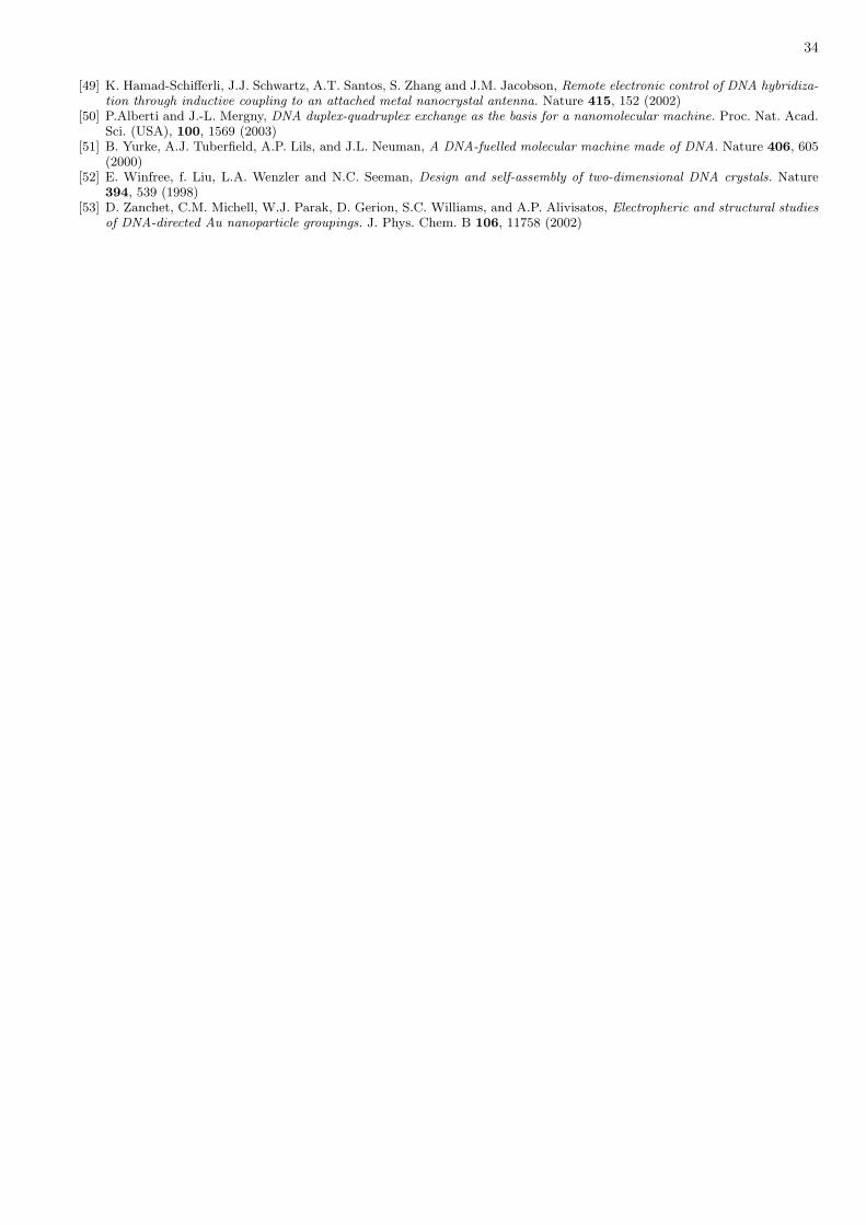
34

[49] K. Hamad-Schifferli, J.J. Schwartz, A.T. Santos, S. Zhang and J.M. Jacobson, Remote electronic control of DNA hybridiza-tion through inductive coupling to an attached metal nanocrystal antenna. Nature 415, 152 (2002)

[50] P.Alberti and J.-L. Mergny, DNA duplex-quadruplex exchange as the basis for a nanomolecular machine. Proc. Nat. Acad.Sci. (USA), 100, 1569 (2003)

[51] B. Yurke, A.J. Tuberfield, A.P. Lils, and J.L. Neuman, A DNA-fuelled molecular machine made of DNA. Nature 406, 605(2000)

[52] E. Winfree, f. Liu, L.A. Wenzler and N.C. Seeman, Design and self-assembly of two-dimensional DNA crystals. Nature394, 539 (1998)

[53] D. Zanchet, C.M. Michell, W.J. Parak, D. Gerion, S.C. Williams, and A.P. Alivisatos, Electropheric and structural studiesof DNA-directed Au nanoparticle groupings. J. Phys. Chem. B 106, 11758 (2002)