IX. Transient Model Nonlinear Regression and Statistical Analysis

Nonlinear Regression

When all K and S parameters are log-transformed, the regression for the transient problem will converge, and

optimal estimates of the nine model parameters will be obtained.

EXERCISE 9.7: Estimate parameters for the transient system by nonlinear regression.

Evaluate Model Fit

Now, we will perform the same analysis of the regression results for the transient problem that was performed for the steady-state problem.

EXERCISE 9.8: Evaluate measures of model fit

Statistical measures of overall model fit, S, s2, and s, are shown in Figure 9.13, p. 246.

Evaluate Model Fit

EXERCISE 9.9: Use Graphs for Analyzing Model Fit and Evaluate Related Statistics

EXERCISE 9.9a: Evaluate graphs of weighted residuals and weighted and unweighted simulated and observed values.

See Figure 9.14, p. 247 of Hill and Tiedeman and

statistic R in Figure 9.13.

Which graphs are most useful to understanding

model fit? Is R helpful?

Weighed Residuals vs. Simulated Values

Figure 9.14a of Hill and Tiedeman (page 247)

-3

-2

-1

0

1

2

-100 -50 0 50 100 150 200

Simulated value

Wei

ghte

d re

sidu

al

Heads

Drawdowns

Flows

Weighted Observed Values vs.Weighted Simulated Values

Figure 9.14b of Hill and Tiedeman (page 247)

-800

-600

-400

-200

0

200

-800 -600 -400 -200 0 200

Weighted simulated value

Wei

ghte

d ob

serv

ed v

alue

Evaluate Model Fit

EXERCISE 9.9b. Evaluate graphs of weighted residuals

against independent variables and the runs statistic.

The runs statistic is given in Figure 9.16, p. 249.

EXERCISE 9.9c: Assess independence and normality

of the weighted residuals.

The normal probability graph and the RN2 statistic are

shown in Figure 9.17, p. 250.

Normal Probability Graph

Figure 9.17 of Hill and Tiedeman (page 250)

-3

-2

-1

0

1

2

3

-3 -2 -1 0 1 2 3

Weighted residual

Stan

dard

nor

mal

sta

tist

icHeads

Drawdowns

Flows

Evaluate Parameter Estimates

EXERCISE 9.10: Evaluate Estimated Parameters

EXERCISE 9.10a. Composite scaled sensitivities.

EXERCISE 9.10b: Parameter estimates and confidence

intervals.

EXERCISE 9.10c: Reasonable parameter ranges.

EXERCISE 9.10d: Parameter correlation coefficients.

CompositeScaled Sens.

258.3

44.3

158.9

0.6 5.3 7.6

53.4

15.7 14.4

0

50

100

150

200

250

300

Q_ 1&2 SS_ 1 HK_ 1 K_ RB VK_ CB SS_ 2 HK_ 2 RCH_ 1 RCH_ 2

PA RA M ETER

CO

MP

OS

ITE

SC

AL

ED

SE

NS

ITIV

ITY

Figure 9.18 of Hill and TiedemanFinal Composite Scaled Sensitivities

(page 251)

197.2

18.2

142.9

0.7 3.2 1.2

41.1

6.317.0

0

50

100

150

200

250

Q_1&2 SS_1 HK_1 K_RB VK_CB SS_2 HK_2 RCH_1 RCH_2

PARAMETER

CO

MPO

SIT

E S

CA

LE

D S

EN

SIT

IVIT

Y

Figure 9.11 of Hill and TiedemanInitial Composite Scaled Sensitivities

(page 243)

ConfidenceIntervals

Figure 9.19 of Hill and Tiedeman:Confidence Intervals for Transient Regression (page 252)Figure 7.7 of Hill and Tiedeman:

Confidence Intervals for Steady State Regression (page 153)

0

100

200

300

400

500

600

700

800

HK_1 K_RB VK_CB HK_2 RCH_1 RCH_2 Q_1&2 SS_1 SS_2

Parameter

Perc

ent o

f est

imat

ed v

alue

Reasonable Range

True value

Starting value

-400

-300

-200

-100

0

100

200

300

400

500

600

HK_1 K_RB VK_CB HK_2 RCH_1 RCH_2

Per

cent

of

estim

ated

val

ue

Reasonable Range

True value

Starting value

Final Parameter Correlation Coefficients

  Q_1&2 SS_1 HK_1 K_RB VK_CB SS_2 HK_2 RCH_1 RCH_2

Q_1&2 1.00 -0.75 -0.99 -0.089 -0.50 -0.056 -0.95 -0.17 -0.91

SS_1   1.00 0.74 -0.19 0.82 -0.60 0.70 0.12 0.68

HK_1     1.00 0.0003 0.51 0.057 0.91 0.18 0.90

K_RB       1.00 -0.38 0.42 0.28 0.005 0.095

VK_CB         1.00 -0.70 0.43 0.090 0.44

SS_2   symmetric       1.00 0.078 0.021 0.065

HK_2             1.00 0.14 0.88

RCH_1               1.00 -0.23

RCH_2                 1.00

Table 9.7 of Hill and Tiedeman (page 253)

Model Linearity

EXERCISE 9.11: Test for linearity.

See Figure 9.20, p. 253.

The modified Beale’s measure is 84.

The model is effectively linear if this measure is less than 0.04, and

the model is nonlinear if this measure is greater than 0.44.

IX. Transient Predictions

Update: Ground-Water Management Issues

Results from the recalibrated model can now be used to update the advective transport predictions.

Many of landfill developer’s concerns have been addressed:

Model has been calibrated with head and flow data collected under same stress conditions that will exist during operation of the landfill, and under which the advective transport will be predicted.

Uncertainty of most flow model parameters has been reduced, compared to their uncertainty in steady-state model.

Advective travel will be analyzed under steady-state pumping conditions, because these are the conditions under which the landfill will operate.

PredictingAdvectiveTransport

Figure 9.21 of Hill and Tiedeman (page 255)

Exercise 9.12a: Plot predicted path

ADVECTIVE-TRANSPORT OBSERVATION NUMBER 1 PARTICLE TRACKING LOCATIONS AND TIMES: LAYER ROW COL X-POSITION Y-POSITION Z-POSITION TIME -------------------------------------------------------------------------------- 1 2 16 15500. 1500.0 100.00 0.0000 ................................................................................ OBS # 1- 3 OBS NAME: AD10 1 2 16 15178. 1575.8 85.940 0.31500E+09 ................................................................................ 1 2 15 15000. 1615.4 79.690 0.47394E+09 1 2 14 14000. 1875.5 56.849 0.12269E+10 1 3 14 13600. 2000.0 51.405 0.14794E+10 2 3 14 13469. 2037.2 50.000 0.15518E+10 PARTICLE ENTERING CONFINING UNIT ................................................................................ OBS # 4- 6 OBS NAME: AD50 2 3 14 13469. 2037.2 48.862 0.15700E+10 ................................................................................ 2 3 14 13469. 2037.2 40.000 0.17114E+10 PARTICLE EXITING CONFINING UNIT 2 3 13 13000. 2167.8 34.419 0.20230E+10 2 3 12 12000. 2539.7 25.685 0.26478E+10 ................................................................................ OBS # 7- 9 OBS NAME: A100 2 3 12 11165. 2909.6 20.380 0.31500E+10 ................................................................................ 2 3 11 11000. 2988.7 19.436 0.32485E+10 2 4 11 10980. 3000.0 19.336 0.32603E+10 2 4 10 10000. 3609.3 14.987 0.38208E+10 2 5 10 9464.0 4000.0 13.057 0.41490E+10 2 5 9 9000.0 4426.0 11.385 0.44536E+10 2 6 9 8497.7 5000.0 10.083 0.48233E+10 2 7 9 8046.1 6000.0 8.1157 0.53184E+10 ................................................................................ OBS # 10- 12 OBS NAME: A175 2 7 9 8018.8 6524.4 6.9647 0.55200E+10 ................................................................................ 2 7 8 8000.0 6988.7 6.1411 0.56728E+10 2 8 8 7999.0 7000.0 6.1113 0.56810E+10 2 8 9 8000.0 7001.1 6.1068 0.56817E+10 2 9 9 8384.8 8000.0 3.0823 0.59752E+10 2 9 10 9000.0 8186.7 1.6827 0.60413E+10

Predicting Advective Transport

Riv

er

Well

Path in original steady-state modelTrue pathPath in updated steady-state model

Landfill

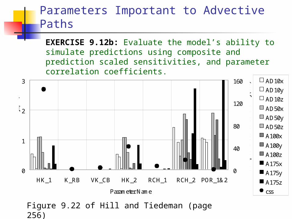
Figure 9.22 of Hill and Tiedeman (page 256)

0

1

2

3

HK_1 K_RB VK_CB HK_2 RCH_1 RCH_2 POR_1&2

Parameter Name

0

40

80

120

160 AD10x

AD10y

AD10z

AD50x

AD50y

AD50z

A100x

A100y

A100z

A175x

A175y

A175z

css

Abs

olut

e va

lue

of p

redi

ctio

n sc

aled

sen

siti

vity

(pss)

Com

posi

te s

cale

d se

nsit

ivit

y (css)

Parameters Important to Advective Paths

EXERCISE 9.12b: Evaluate the model’s ability to simulate predictions using composite and prediction scaled sensitivities, and parameter correlation coefficients.

  Q_1&2 SS_1 HK_1 K_RB VK_CB SS_2 HK_2 RCH_1 RCH_2

Q_1&2 1.00 -0.75 -0.99 -0.089 -0.50 -0.056 -0.95 -0.17 -0.91

SS_1   1.00 0.74 -0.19 0.82 -0.60 0.70 0.12 0.68

HK_1     1.00 0.0003 0.51 0.057 0.91 0.18 0.90

K_RB       1.00 -0.38 0.42 0.28 0.005 0.095

VK_CB         1.00 -0.70 0.43 0.090 0.44

SS_2   symmetric       1.00 0.078 0.021 0.065

HK_2             1.00 0.14 0.88

RCH_1               1.00 -0.23

RCH_2                 1.00

  Q_1&2 SS_1 HK_1 K_RB VK_CB SS_2 HK_2 RCH_1 RCH_2

Q_1&2 1.00 -0.65 -0.99 -0.066 -0.40 -0.035 -0.92 -0.37 -0.84

SS_1   1.00 0.63 -0.26 0.80 -0.71 0.58 0.22 0.53

HK_1     1.00 -0.050 0.42 0.036 0.84 0.38 0.82

K_RB       1.00 -0.43 0.42 0.32 0.016 0.076

VK_CB         1.00 -0.75 0.30 0.15 0.32

SS_2   symmetric       1.00 0.063 0.028 0.047

HK_2             1.00 0.31 0.79

RCH_1               1.00 -0.17

RCH_2                 1.00

Table 9.7 of Hill and Tiedeman: without predictions

Table 9.8 of Hill and Tiedeman: with predictions

Prediction Uncertainty:Linear Simultaneous Confidence Intervals

10 yrs

50 yrs

100 yrs

175 yrs

Riv

er

Well

True particleposition at:

Predicted pathConfidence intervalTrue path

50 yr100 yr

10 yr

175 yr

Fig 8.15b, p. 210

From calibration with

transient data

From calibration with steady-state data

50 yr

Riv

er

Well

100 yr

10 yr

Fig 9.23a, p. 258

EXERCISE 9.12c: Evaluate prediction uncertainty using inferential statistics.

Riv

er

Well

50 yr100 yr

10 yr

175 yr

Fig 8.15d, p. 210 Fig 9.23d, p. 258

From calibration with

transient data

From calibration with steady-state data

Prediction Uncertainty:Nonlinear Simultaneous Confidence Intervals

50 yr

Riv

er

Well

100 yr

10 yr

Finally:

Should the landfill be approved?

Why or why not?