Embed Size (px)
Citation preview

STAT 8230 — Applied Nonlinear RegressionLecture Notes
Linear vs. Nonlinear Models
Linear regression, analysis of variance, analysis of covariance, and most ofmultivariate analysis are concerned with linear statistical models.
These models describe the dependence relationship between one or morecontinuously distributed response random variables and a set of explanatoryvariables or factors.
• These models are parametric because, when fully specified, theyassume that the probability distribution of the response variable(s),including a model for the dependence between response and explana-tory variables, is known except for the values of a small number ofunknown constants called parameters.
• These models are linear in the sense that the regression parameters(the parameters that describe the dependence of the mean responseon explanatory variables) enter into the models linearly.
– The model is linear in the parameters, not the explanatory vari-ables.
1

For example, the following is the general form of the classical multipleregression model:
yi = β1xi1 + β2xi2 + · · ·+ βpxip + ei, i = 1, . . . , n,
and e1, . . . , eniid∼ N(0, σ2)
(∗)
• Here, we assume that we have a random sample of n observations(yi, xi1, . . . , xip), i = 1, . . . , n, of a response variable Y and a set of pexplanatory variables X1, . . . , Xp.
• In addition, the notationiid∼ N(0, σ2) means, “are independent, iden-
tically distributed random variables each with a normal distributionwith mean 0 and variance σ2.”
• Typically, xi1 is equal to one for all i in multiple linear regressionmodels, but this need not be so.
• In model (*) the parameters are β1, . . . , βp, σ2. The regression param-
eters are β1, . . . , βp.
In regression models, the explanatory variables (xi1, . . . , xip, i = 1, . . . , n,above) are treated as nonrandom, either by assumption that they have beenset to their observed values by design or some other nonrandom mechanism,or, more generally, by making the model conditional on the observed Xvales.
• That is, regression models specify the conditional distribution of Y |X1, . . . , Xp.In particular, regression models are primarily concerned with themean of this distribution: E(Y |X1, . . . , Xp).
• E(Y |X1, . . . , Xp), the conditional expectation of the response giventhe values of the explanatory variables, is known as the regressionfunction.
– Since we always condition on the explanatory variables in linearand nonlinear regression models, we will often drop the condi-tioning from the notation for convenience and write E(Y ) inplace of E(Y |X1, . . . , Xp).
2

In the multiple linear regression model (*), the regression function for theith subject (unit of observation), call it µi, is
µi ≡ E(yi) = E(β1xi1 + β2xi2 + · · ·+ βpxip + ei)
= β1xi1 + β2xi2 + · · ·+ βpxip + E(ei)︸ ︷︷ ︸=0
= β1xi1 + β2xi2 + · · ·+ βpxip
Notice that the regression parameters β1, . . . , βp enter into the regressionfunction in a linear fashion.
• Recall that a linear combination of z1, . . . , zk is a weighted sum a1z1+a2z2 + · · ·+ akzk of the zj ’s with coefficients a1, . . . , ak.
• Of course, the multiple linear regression model is linear in the βj ’sand in the xji’s, but the fact that it is linear in the βj ’s is what makesit a linear model.
In this course, a nonlinear regression model is still going to be a regres-sion model describing the relationship between a continuously distributedresponse variable yi and explanatory variables xi1, . . . , xip, but now we dropthe linearity assumption,
µi = β1xi1 + · · ·+ βpxip,
and allow the parameters θ1, . . . , θp and explanatory variables xi1, . . . , xikto enter into the regression function in a nonlinear way.
• Notice we’ve switched to calling the parameters θ’s instead of β’s. Inaddition, the number of explanatory variables, k, is not necessarilyequal to the number of parameters, p.
3

That is, in the nonlinear regression models under study in this course,µi = f(xi1, . . . , xik, θ1, . . . , θp), where f(·) is a function not necessarily linearin the θ’s. Otherwise, the model is the same:
yi = f(xi1, . . . , xik, θ1, . . . , θp) + ei, i = 1, . . . , n,
where e1, . . . , eniid∼ N(0, σ2)
(∗∗)
• Note that we’ve restricted attention here somewhat in the class of allpossible not-linear models. We retain the assumption of a continuousresponse, additive error, and (usually) normally distributed errors.
• Excluded from consideration are several important classes of regres-sion models that are nonlinear in some sense.
– In particular, we exclude generalized linear models (GLMs, e.g.,logistic regression models, Poisson loglinear models, etc.) Manycases of GLMs are for discrete data, and GLMs retain a (modi-fied) linearity in the parameters assumption.
4

Example — Onion Data:
The following table and scatterplot display data on the dry weight (Y ) of 15onion bulbs randomly assigned to 15 growing times (X) until measurement.
Growing Time Dry Weight Growing Time Dry Weight
1 16.08 9 590.032 33.83 10 651.923 65.8 11 724.934 97.2 12 699.565 191.55 13 689.966 326.20 14 637.567 386.87 15 717.418 520.53
••
••
•
•
•
•
•
•
•• •
•
•
Growing Time
Dry
Wei
ght
2 4 6 8 10 12 14
020
040
060
0
5

Suppose we wanted to fit a model to describe how the mean dry weightof onions depends upon growing time. From the data and scatterplot, itis clear that weight tends to increase with growing time in a nonlinear (ingrowing time) fashion.
However, a linear (in the parameters) model can still be used to capture thisnonlinear pattern of growth by considering polynomial models in growingtime. That is, consider models of the form
yi = β1 + β2xi + β3x2i + · · ·+ βpx
p−1i + ei, i = 1, . . . , n,
where e1, . . . , en are i.i.d. each with mean 0, and variance σ2 (constantvariance).
Alternatively, we might consider a nonlinear model. In particular, considerthe 3-parameter logistic model (a.k.a. simple logistic model):
yi =θ1
1 + exp{(θ2 − xi)/θ3}+ ei, i = 1, . . . , n,
with the same assumptions on the ei’s.
How do we choose between a linear model (e.g., polynomial in growingtime) and a nonlinear model (e.g., simple logistic model) in this problem?
From a purely empirical point of view, we might choose the model that fitsthe data most closely.
However, we need to be a little bit careful here to balance fit against par-simony and generality. If we include enough terms in a polynomial modelwe can fit the data perfectly.
6

In particular, a (n− 1)th degree polynomial can fit n points exactly. Sucha model has n parameters and is equivalent to (is just a reparameterizationof) the model
yi = βi + ei, i = 1, . . . , n. (†)
Such a model clearly doesn’t summarize or simplify the data at all andcan’t be expected to generalize beyond the particular features of this onerandomly drawn data set.
• In addition, a model such as (†) leaves no degrees of freedom left toestimate error variance ⇒ can’t do inference (test hypotheses, formconfidence intervals) based on the model.
If we think of each of the n observations as an independent piece of informa-tion (or degree of freedom) from which to fit a model, then we use up one ofthese pieces of information (degrees of freedom) for every (nonredundant)parameter estimated in the model.
• n regression parameters to be estimated ⇒ n d.f. used to estimatethe model (model d.f.) ⇒ n − n = 0 d.f. left to estimate the errorvariance parameter σ2 (0 d.f. for error).
The smaller the number of regression parameters in the model, the mored.f. available to estimate error variance ⇒ more power for hypothesis tests,more precision in confidence intervals.
• Parsimonious models that fit the main features of the data are pre-ferred.
Consider the fits of the simple logistic model and polynomial models oforder 2, 3, and 4 to the onion data on the following page.
7

••
••
•
••
••
••
••
••
Gro
win
g T
ime
Dry Weight
24
68
1012
14
0200400600
3-pa
ram
eter
logi
stic
mod
el (
nonl
inea
r)
••
••
•
••
••
••
••
••
Gro
win
g T
ime
Dry Weight
24
68
1012
14
0200400600
3-pa
ram
eter
line
ar m
odel
••
••
•
••
••
••
••
••
Gro
win
g T
ime
Dry Weight
24
68
1012
14
0200400600
4-pa
ram
eter
line
ar m
odel
••
••
•
••
••
••
••
••
Gro
win
g T
ime
Dry Weight
24
68
1012
14
0200400600
5-pa
ram
eter
line
ar m
odel
8

• Notice that it requires a less parsimonious (more parameters) linearmodel to fit the main features of the data than for a nonlinear model.
• In addition, while the quadratic (3 parameter linear) model clearlyunderfits the general shape of the curve, the cubic and quartic linearmodels appear to overfit the data.
• So, from a purely empirical point of view, the logistic model appearspreferrable.
• In addition, the logistic model has a big advantage in terms of param-eter interpretability for a growth model such as this one.
Interpretations of the parameters in the simple logistic model:
x
y
φ1
φ2
φ3
FIGURE C.7. The simple logistic model showing the parameters φ1, the horizon-tal asymptote as x→ ∞, φ2, the value of x for which y = φ1/2, and φ3, a scale
parameter on the x-axis. If φ3 < 0 the curve will be monotone decreasing instead
of monotone increasing and φ1 will be the horizontal asymptote as x→ −∞.
9

• θ1 (ϕ1 in the plot on the previous page) represents the asymptote ofthe curve (limit of onion weight as growth time increases toward itsmaximum value).
• θ2 represents the x-value at which y is equal to θ1/2, one-half of itsasymptotic value. The growth time at which onions have achievedhalf of their total potential weight.
• θ3 is a scale parameter that does not have as natural of an interpre-tation.
• In contrast, the polynomial parameters are not as meaningful to thecontext of the problem.
So fit, parsimony, and parameter interpretability can point to using non-linear models over linear ones. A further important motivation for usingnonlinear models over linear ones is subject matter theory.
• It may be that we have a mechanistic theory that explains the natureof onion growth and which implies a nonlinear functional form forthe relationship between weight (or some other measure of size) andgrowing time.
• We will see plenty of examples of theoretically motivated nonlinearmodels as the course progresses.
10
Review of Linear Regression Models
Before discussing nonlinear regression we need to review linear regression.
Why?
• Because many of the ideas and methods from linear regression transferdirectly or with minor modification to the nonlinear case.
• And because many of the methods of estimation and inference inNLMs are linear methods applied to a linear approximation to theNLM.
Again, we assume that we observe a sample of independent pairs, (y1,x1), . . . ,(yn,xn) where yi is a response variable and xi = (xi1, . . . , xip)
T is a p × 1vector of explanatory variables (assumed fixed).
The classical linear model can be written
yi = β1xi1 + · · ·+ βpxip + ei, i = 1, . . . , n,
= xTi β + ei,
where e1, . . . , eniid∼ N(0, σ2). Equivalently, we can stack these n equations
and write the model as follows: y1...yn
=
x11 x12 · · · x1p...
.... . .
...xn1 xn2 · · · xnp
β1
...βp
+
e1...en
or y = Xβ + e
Our assumptions on e1, . . . , en can be equivalently restated as
e ∼ Nn(0, σ2In),
where Nn(µ,M) denotes the n−dimensional multivariate normal distribu-tion with mean µ and variance-covariance matrix M.
11

Multivariate normal distribution:
The multivariate normal distribution is to a random vector (vector of ran-dom variables) as the univariate (usual) normal distribution is to a randomvariable. It is the version of the normal distribution appropriate to the jointdistribution of several random variables (collected and stacked as a randomvector) rather than the distribution of a single random variable.
• E.g., for a bivariate random vector x =
(x1x2
)that has a bivariate
normal distribution, the density function of x maps out a bell overthe (x1, x2) plane.
The Nn(µ,Σ) distribution is completely described by the two parametersµ, the mean of the distribution, and Σ, the variance-covariance matrixof the distribution.
• That is, for x = (x1, x2, . . . , xn)T ∼ Nn(µ,Σ),
µ =
E(x1)E(x2)
...E(xn)
, and Σ =
var(x1) cov(x1, x2) · · · cov(x1, xn)
cov(x2, x1) var(x2) · · · cov(x2, xn)...
.... . .
...cov(xn, x1) cov(xn, x2) · · · var(xn)
describe the location and dispersion (spread), respectively, of the bell-shaped distribution of possible values for x.
12

The probability density function (p.d.f.) of x generalizes the univariatenormal p.d.f.
• Recall for X ∼ N(µ, σ2) the p.d.f. of X is
f(x) =1
(2πσ2)1/2exp
{−1
2
(x− µ)2
σ2
}, −∞ < x <∞
• In the multivariate case, for x ∼ Nk(µ,Σ), the p.d.f. of x is
f(x) =1
(2π)k/2|Σ|1/2exp
{−1
2(x− µ)TΣ−1(x− µ)
}, x ∈ Rk.
– Here |Σ| denotes the determinant of the var-cov matrix Σ.
In the CLM, since e ∼ Nn(0, σ2In) and y = Xβ+e, it follows that y ∼ Nn
too, with mean
E(y) = E(Xβ + e) = Xβ + E(e)︸︷︷︸=0
= Xβ
and var-cov matrix
var(y) = var(Xβ + e)
= var(e) = σ2
1 0 · · · 00 1 · · · 0...
.... . .
...0 0 · · · 1
=
σ2 0 · · · 00 σ2 · · · 0...
.... . .
...0 0 · · · σ2
.(∗)
• Assumption (*) says that the yi’s are uncorrelated (cov(yi, yi′) = 0,for i = i′) and have constant variance (var(y1) = · · · = var(yn) = σ2).
13

So, the assumptions of the CLM can be stated quite succinctly as:
y ∼ Nn(Xβ, σ2In). (†)
Therefore, in the CLM y is assumed to have the joint p.d.f.
f(y;β, σ2) =1
(2π)n/2|σ2In|1/2exp
{−1
2(y −Xβ)T (σ2In)
−1(y −Xβ)
}= (2πσ2)−n/2 exp
{− 1
2σ2(y −Xβ)T (y −Xβ)
}
= (2πσ2)−n/2 exp
− 1
2σ2∥y −Xβ︸ ︷︷ ︸
=e
∥2 , y ∈ Rk.
• Here, ∥v∥ =√vTv denotes the norm, or length, of the vector v.
Therefore, ∥y −Xβ∥ denotes the length of the difference between yand Xβ; i.e., the (Euclidean) distance between y and Xβ.
• (Note that we’ve used here the fact that the determinant of a diagonalmatrix (a matrix whose off-diagonal elements are all 0) is the productof the diagonal elements ⇒ |σ2In| = σ2n.)
• Actually, many of the results in the theory of linear models canbe established with the weaker assumptions obtained by droppingnormality from (†); that is, under the assumptions E(y) = Xβ,var(y) = σ2In and y1, . . . , yn are independent.
• As mentioned previously, the mean of y (conditional onX) is known asthe regression function or (as we’ll call it) the expectation functionof the model. In the linear regression model, the expectation functionis E(y) = Xβ.
14

Notice that in the linear model,
∂E(yi)
∂βj=∂(xT
i β)
∂βj=∂(xi1β1 + · · ·+ xipβp)
∂βj= xij
To denote the derivative of the vector µ = E(y) with respect to the vectorβ we use the notation
∂µ
∂βT=
∂µ1
∂βT
∂µ2
∂βT
...∂µn
∂βT
=
∂µ1
∂β1
∂µ1
∂β2· · · ∂µ1
∂βp
∂µ2
∂β1
∂µ2
∂β2· · · ∂µ2
∂βp
· · ·...
. . ....
∂µn
∂β1
∂µn
∂β2· · · ∂µn
∂βp
• So we see that the derivative of Xβ with respect to β gives the matrixX. For this reason X is called the derivative matrix.
– Note thatX is also sometimes called themodel matrix, or designmatrix in linear models.
– In linear regression notice that the derivative matrix∂µ∂βT
does
not depend on β. This will not be the case in nonlinear regres-sion.
15

Estimation of β and σ2:
Maximum likelihood estimation:
In general, the likelihood function is just the probability density function,but thought of as a function of the parameters rather than of the data.
• For Example, in the CLM, the p.d.f. of the response variable y is
f(y;β, σ2) = (2πσ2)−n/2 exp
{− 1
2σ2∥y −Xβ∥2
}
– This p.d.f. is a function of the observed response y and theparameters β and σ2, but we think of it primarily as a functionof y.
– In the discrete case, the p.d.f. gives the probability of observingits argument, the data (y above), for given values of the param-eters. In the continuous case the interpretation is very similar,but slightly more complicated.
Since the p.d.f. involves both the parameters (β and σ2) and the data(y), once the data are observed, we can think of it as a function of theparameters given the data.
This re-interpretation of the density function is given a new name, thelikelihood function, and written as primarily a function of the parameters.
E.g., in the CLM the likelihood function is
L(β, σ2;y) = (2πσ2)−n/2 exp
{− 1
2σ2∥y −Xβ∥2
}
16

• The idea behind maximum likelihood estimation is to find the valuesof β and σ2 under which the data are most likely. That is, we findthe β and σ2 that maximize the likelihood function (and p.d.f.) forthe value of y actually observed. These values are the maximumlikelihood estimators (MLEs) of the parameters.
• Note that since the natural logarithm is an increasing function, maxi-mizing L(β, σ;y) with respect to the parameters is equivalent to (pro-duces the same answer as) maximizing ℓ(β, σ2;y) ≡ log{L(β, σ2;y)}.Since taking logarithms is often mathematically convenient and itdoesn’t change the probelm, we’ll typically work with this loglikeli-hood function rather than the likelihood function.
For the CLM, the loglikelihood is
ℓ(β, σ2;y) = −n2log(2π)︸ ︷︷ ︸
a constant
−n2log(σ2)− 1
2σ2∥y −Xβ∥2︸ ︷︷ ︸
kernel of ℓ
.
• Note that it is equivalent to maximize the kernel of the loglikelihood— that portion of the loglikelihood depending upon the parameters.Terms not involving the parameters can be ignored.
Obtaining the MLEs in the CLM: This can be done in two steps
1. Maximize ℓ(β, σ2;y) with respect to β, treating σ2 as known. Call
the resulting estimator β.
2. Then maximize ℓ(β, σ2;y) with respect to σ2. Call the resulting esti-mator σ2.
Then β, σ2 will be the MLEs of β, σ2.
17

1. In step 1 we treat σ2 as known and maximize ℓ(β, σ2;y) with respectto β. Note that this is equivalent to maximizing the third term,
− 1
2σ2∥y −Xβ∥2,
which is equivalent to minimizing
∥y −Xβ∥2 = ∥e∥2 =n∑
i=1
e2i =n∑
i=1
(yi − xTi β)
2 ≡ S(β). (∗)
• Thus the MLE of β minimizes S(β), which is known as the leastsquares criterion.
– So, the estimators of β given by ML and least squares coincide.
We can obtain the MLE/LSE, β, by solving the normal equationswhich are obtained by differentiating S(β) and setting the result equalto 0.
S(β) can be written
S(β) = (y −Xβ)T (y −Xβ) = yTy − yTXβ − βTXTy︸ ︷︷ ︸=yTXβ
+βTXTXβ
= yTy − 2yTXβ + βTXTXβ
• Need ∂S
∂βT.
18

To take the necessary derivatives, we need some results on matrixdifferentiation. For x a vector and A a matrix,
i. ∂Ax∂xT = A.
ii. ∂xTAx∂xT = 2xTA.
Using (i) and (ii) we get
∂S
∂βT= −2yTX+ 2βTXTX
so that the normal equations become
2βTXTX = 2yTX
or XTXβ = XTy.
If XTX is invertible (nonsingular) we can multiply through on bothsides by (XTX)−1 to give the MLE/Least squares estimator of β as:
β = (XTX)−1XTy. (‡)
• We’ll assume (XTX) is invertible henceforth unless stated otherwise.Note that if (XTX) is not invertible a (no longer unique) estimatorof β is obtained simply by replacing the matrix inverse in (‡) with ageneralized matrix inverse.
19

2. Now we maximize ℓ(β, σ2;y) with respect to σ2. Taking derivativeswith respect to σ2 we get
∂ℓ
∂(σ2)=
−n/2σ2
+(1/2)∥y −Xβ∥2
σ4= 0,
which has solution,
σ2 =1
n∥y −Xβ∥2 =
1
n
n∑i=1
(yi − xTi β)
2.
• We will see that β has a number of desirable properties includingsome optimality properties. However, σ2 is not typically the preferredestimator.
One fault with σ2 is that it is biased. It can be shown that
E(σ2) =n− p
nσ2
Therefore, an unbiased estimator that is generally superior to σ2 canbe formed by taking
n
n− pσ2 =
1
n− p∥y −Xβ∥2 =
1
n− p
n∑i=1
(yi − xTi β)
2 ≡ s2
• We call this estimator s2, the mean squared error.
20

Properties of β and methods of inference on β:
Several properties of β follow from the fact that it is a linear function of y.
(That is, β = (XTX)−1XTy is of the form My for M a matrix ofconstants.)
This linearity combined with the model equation y = Xβ+e leads to somenice, simple properties.
Notice,
β = (XTX)−1XTy = (XTX)−1XT (Xβ + e)
= (XTX)−1XTXβ + (XTX)−1XTe
= β + (XTX)−1XTe
It follows that
1. β is unbiased, since
E(β) = E{β + (XTX)−1XTe} = β + (XTX)−1XT E(e)︸︷︷︸=0
= β.
2. β has var-cov matrix
var(β) = var{β + (XTX)−1XTe} = var{(XTX)−1XTe}= (XTX)−1XT var(e)︸ ︷︷ ︸
=σ2I
X(XTX)−1 = σ2(XTX)−1
( Here we’ve used that fact that if w is a n × 1 random vectorwith var-cov matrix Σ and B is an m × n matrix of constants,then var(Bw) = Bvar(w)BT = BΣBT .)
3. (normality) β ∼ Np(β, σ2(XTX)−1) (if e is assumed normal).
21

4. β is the Best (minimum variance) estimator in the class of all Linear
Unbiased Estimators (β is BLUE). This result doesn’t require theassumption of normality on the errors of the CLM.
5. Under the assumption of normal errors, β and s2 are minimum vari-ance unbiased estimators (best in the class of unbiased, but not-necessarily linear estimators).
6. Since var(β) = σ2(XTX)−1 (by (2)), var(βj) = σ2(XTX)−1jj . Since σ
2
is typically unknown, we must estimate it with s2 to get an estimate ofvar(βj). The square root of this estimated variance is the standard
error of βj :
s.e.(βj) = s√(XTX)−1
jj .
With this standard error in hand, methods of inference (hypothesistests, confidence intervals) follow from the fact that
βj − βj
s.e.(βj)∼ t(n− p)︸ ︷︷ ︸
the t distribution with n− p d.f.
– ⇒ βj ± t1−α/2(n − p)s.e.(βj) forms a 100(1 − α)% marginalconfidence interval for βj .
– For an α-level test of H0 : βj = β0 versus H1 : βj = β0 we usethe rule: reject H0 if
|βj − β0|s.e.(βj)
> t1−α/2(n− p)
22

7. Inference on the entire vector β is based on the fact that
(β − β)T (XTX)(β − β)ps2
∼ F (p, n− p)︸ ︷︷ ︸the F distribution with p and n− p d.f.
– A 100(1− α)% joint confidence region for β is given by theset of all β such that
(β − β)T (XTX)(β − β)ps2
≤ F1−α(p, n− p)
This region consists of the surface and interior of an ellipsoid(p-dimensional ellipse; e.g., a watermelon for p = 3).
– For an α-level test, we rejectH0 : β = β0 in favor ofH1 : β = β0
if(β − β0)
T (XTX)(β − β0)
ps2> F1−α(p, n− p).
– The previous result is sometimes of use when β0 = 0, but oftenwe want to test that some linear function of β (e.g., a subvectorof β) is equal to 0 or some other null value b. In that case, itis useful to have a generalization of the above F test for H0 :Aβ = b versus H1 : Aβ = b where A is a k × p matrix ofconstants and b is a k× 1 vector of constants. The appropriatetest has rejection rule: reject if
F =(Aβ − b)T {A(XTX)−1A}−1(Aβ − b)
ks2> F1−α(k, n− p).
(Note that not every such hypothesis is testable. We requirethat A has full row rank. Essentially, this means there is noredundancy in the statement of the null hypothesis.)
23

8. A 100(1− α)% C.I. for the expected response at a given value of thevector of explanatory variables xo is given by
xT0 β ± t1−α/2(n− p)
√s2xT
0 (XTX)−1x0.
– Similarly, we can form a C.I. for any linear combination of theβ’s that can be written in the form cTβ for c a vector of con-stants by replacing x0 with c. A 100(1 − α)% C.I. for cTβ isgiven by
cT β ± t1−α/2(n− p)√s2cT (XTX)−1c.
9. A 100(1−α)% C.I. for the predicted response (not the mean responseover the population, but a single new observation of the responsevariable) at a given value of the vector of explanatory variables xo isgiven by
xT0 β ± t1−α/2(n− p)
√s2[1 + xT
0 (XTX)−1x0].
• Such an interval is usually called a prediction interval ratherthan a confidence interval.
10. A 100(1− α)% confidence band for the response function at any xis given by
xT β ±√F1−α(p, n− p)
√ps2xT (XTX)−1x.
• Result (8) gives a C.I. at a single given point (x0) whereas re-sult (10) gives a confidence band that holds for all values of xconsidered simultaneously.
24

Example – PCB in Trout (fitting a linear model in R):
The data below consist of PCB (polychlorinated biphenyls, a toxin) con-centrations in Lake Cayuga (NY) trout of various ages.
Age PCB Conc. Age PCB Conc.(years) (ppm) (years) (ppm)
1 0.6 6 3.41 1.6 6 9.71 0.5 6 8.61 1.2 7 4.02 2.0 7 5.52 1.3 7 10.52 2.5 8 17.53 2.2 8 13.43 2.4 8 4.53 1.2 9 30.44 3.5 11 12.44 4.1 12 13.44 5.1 12 26.25 5.7 12 7.4
• See the handout labelled trout1. The first page of this handout con-tains R commands contained in the R script file trout1.R. Pages 2–3contain the text output of these commands and p.4 the graphics out-put.
• The first plot p.4 of trout1 contains a scatterplot of PCB concentrationversus age. From the plot there appears to be some nonlinearity inage and heteroscedasticity (nonconstant, in this case increasing withage, variance).
• From these observations it appears that the assumptions of the CLMpreclude its use here. However, transformations of the response andexplanatory variables can often induce linearity, normality and con-stant variance thereby making the CLM an appropriate tool.
25

• One useful class of transformations is the Box-Cox family of powertransformations:
g(Y ;λ) =
{Y λ−1
λ , if λ = 0log Y, if λ = 0
– For CLMs with an intercept term, this family is equivalent tothe “simple” family of power transformations given by
gS(Y ;λ) =
{Y λ, if λ = 0log Y, if λ = 0
but the Box-Cox family is slightly more convenient mathemati-cally.
• The specific transformation in the Box-Cox family can be chosen byestimating λ by ML estimation. Box and Cox showed that the MLestimator (MLE) of λ can be obtained as the maximizer of the function
−n2log SSE{z(λ)},
where z(λ) has ith element g(yi;λ)/yλ−1, y is the geometric mean of
the elements of y and SSE{z(λ)} denotes the error sum of squares forthe regression of z(λ) on X.
– This function is known as the profile likelihood for λ.
26

• Therefore, it is possible to obtain the MLE of λ by plotting
−n2log SSE{z(λ)}
over a range of λ values and selecting the λ-value that maximizes thisfunction. This is automated in the boxcox macro in R (part of theMASS package).
• See trout1.R. trout1.R contains R commands to select the appropriatetransformation of PCB concentration and then to fit a linear regres-sion model to the transformed data. These commands also producethe plots on p.4 of trout1.
• The boxcox macro is part of the MASS (Modern Applied Statisticswith S-PLUS — the book by Venables and Ripley mentioned in thesyllabus) library. This library comes standard with R, but must beloaded into an R session with the library(MASS) command.
• The par(mfrow=c(2,3)) command sets the graphical parameter mfrowso that plots are laid out 2× 3 on a page.
• boxcox plots the profile likelihood for λ (see p.4 of trout1 handout,
top-middle plot). From this plot we see that the MLE λ is close to
0. Rather than using the exact MLE, its preferable to round λ to thenearest interpretable value (e.g., 0, 1/4, 1/3, 1/2). In this case wetake λ = 0 and use the log transformation.
• A plot of log(PCB Conc.) against age looks much more linear andhomoscedastic. A cube-root transformation of age improves the sit-uation even further (we omit discussion of selecting transformationsof the explanatory variables, but this subject is discussed in Box andTidwell (1962) and elsewhere).
27

• A linear regression of the form
yi = β1 + β2xi + ei, i = 1, . . . , 28,
where e1, . . . , e28iid∼ N(0, σ2) and yi = log(PCB), xi = age
1/3i is fit
using the lm function. The “data frame” trout contains the variableson their original scale. The I() function just allows the computationof the transformation to be done within the call to lm.
• R is an object-oriented language. This means that quite complicatedentities like model fits can be stored and operated on as a singleobject. E.g., m1trout.lm is assigned the entire model fit. It is storedas a list containing all of the results of the model fit listed by thefunction names(m1trout.lm). The fitted model can be summarizedwith the command summary(m1trout.lm) and various other functions(like coef) exist for extracting results from m1trout.lm.
• The remainder of the code in trout1.R computes confidence intervalsand regions for β and produces the rest of the plots on p.4 of trout1.
• For example, we can obtain the 95% confidence band for the averagelog(PCB) value at all x (values of age1/3) by plotting
( 1 x )
(β1β2
)±
√F.95(2, 28− 2)
√2s2 ( 1 x ) (XTX)−1
(1x
)or (−2.391 + 2.300x)±
√3.369
√2(.246)(.637− .718x+ .214x2)
over the range of x-values observed in the data.
28

The Geometry of Linear Least Squares:
Again, let S(β) = ∥y − Xβ∥2, the squared (Euclidean, or straight-line)distance from y to its mean according to the model, Xβ.
• The linear least squares estimator β minimizes S(β).
Calculating S(β) consists of 2 steps:
1. Using the n× p derivative matrix X and the p × 1 parameter vectorβ to form the expected response vector η(β) = Xβ.
2. Calculating the squared distance from the expected response η(β) tothe observed response y.
• Though η(β) lies in n−space (has n components), the set of all pos-sible values it can take is not n−space. We can only vary the pparameters in β to get different values of η(β). That is, η(β) lies ina p-dimensional subspace of n−dimensional space.
• We call the set of all possible values of η(β) the expectation surfaceof the model.
– In a linear model, η(β) = Xβ is a linear combination of thecolumns of X (Xβ = β1x1 + · · · + βpxp where xj is the jth
column of X) so we call the Xβ the expectation plane of themodel.
29

Very Simple Example — n = 2, p = 1:
Suppose we have a response vector with just two components: y =
(42
)to which we’d like to fit the linear model
yi = β + ei, i = 1, 2
or
y = βx+ e, where x =
(11
).
The response vector y falls in two-dimensional space. We can plot y asfollows:
• Least-squares estimate of β: the β so that η(β) is the closest pointon the expectation plane to y.
– Since η(β) =
(33
)is the closest point to y =
(42
)it is easy
to find that the β that yields β
(11
)=
(33
)is β = 3.
30

A Slightly Less Simple Example — n = 3, p = 2:
Consider again the PCB in trout data and suppose we want to fit our simplelinear regression model as before
yi = β1 + β2xi + ei, i = 1, . . . , n
for y = log(PCB) and x = age1/3, but now suppose we have only n = 3observations:
age1/3 log(PCB)
1.26 0.921.82 2.152.22 2.52
The derivative matrix here is
X =
1 1.261 1.821 2.22
with columns x1 = (1, 1, 1)T and x2 = (1.26, 1.82, 2.22)T .
31
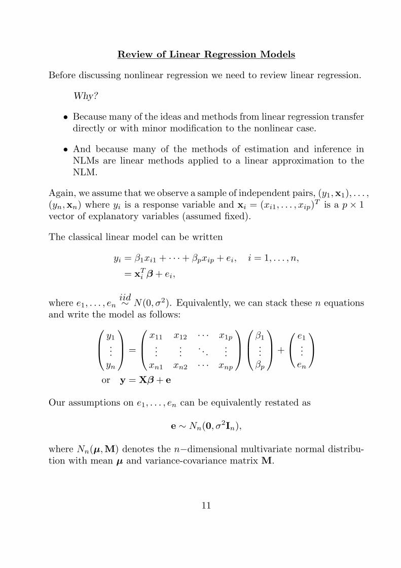
• Since the response has n = 3 components, the response space is3−dimensional space. We can plot x1 and x2 in that space (below,plot (b)).
• The expectation plane is the set of all η such that η = β1x1+β2x2 forsome constants β1 and β2. This plane is depicted in plot (c) above.
• η(β) is the point on this plane that is closest to y = (0.92, 2.15, 2.52)T
(it is the (Euclidean) projection of y onto that plane).
• β is the value of β that yields this closest point to y.
32

So, to find β we
1. Find η that is closest to y; then
2. find β such that η(β) = η.
We know from differentiating the least squares criterion that β solves thenormal equation
(XTX)β = XTy (∗)
• Another way we can derive (*) is from the geometry of the problem:
– The expectation plane is the set of all n× 1 vectors that can bewritten as Xa for some p × 1 vector a (the set of all possiblelinear combinations of the columns of X).
– We know that the residual vector y − Xβ must be orthogo-nal (i.e., perpendicular) to the expectation plane, so the angle
between y −Xβ and Xa must be 90◦ for any p× 1 vector a.
– Algebraically, two vectors b and c form a 90◦ angle if and onlyif their inner product bT c equals 0.
– Therefore, the geometry of least squares implies that the leastsquares estimator of β satisfies
(y −Xβ)T (Xa) = 0, for all a
or yTXa = βTXTXa, for all a
which implies yTX = βTXTX,
or, equivalently, XTy = XTXβ, (the normal equation)
and again we obtain that β must satisfy the normal equation.
33

Assumptions of the CLM:
Model:y = Xβ + e, e ∼ Nn(0, σ
2In).
1. Expectation function is correctly specified as E(y) = Xβ. Expecta-tion form assumed linear in β and contains all important predictorvariables each on the right scale.
2. Additive error. We assume y = Xβ + e rather than, for example,yi = (xT
i β)ei . This assumption implies
– Distribution of y −Xβ doesn’t depend on β.
– β should be estimated to make y −Xβ “small.”
3. The distribution of e does not depend on X. That is, the effect of Xon y is completely captured by Xβ. Often justified by randomization.
4. Each ei has mean 0. This is a consequence of (1) and (2). Not atall restrictive in a linear model with intercept, but deserves someattention in a nonlinear model with no intercept.
5. Homoscedasticity. Each ei has the same variance, σ2. Implies y1, . . . , ynall have the same variance, σ2.
6. Independence. The ei’s are independent ⇒ the yi’s are independent.Often justified by randomization.
7. Normality. Assume each ei follows a normal (Gaussian) distribution.
• Assumptions (4)–(7) imply that the length of y−Xβ should be mea-sured with Euclidean distance: ∥y −Xβ∥.
• Assumption (7) is not necessary to motivate least-squares and estab-lish its optimality (BLUE-ness). However, classical inference methodsrely on (7).
34

Model fitting is an iterative process: Make assumptions. Fit model. Checkassumptions. Revise model. Check revised model’s assumptions. Etc.
Verifying the Assumptions:
Since most of the assumptions are made on the error terms, it makes senseto check whether these assumptions appear to hold for the estimated errorterms, or residuals.
Let y = Xβ be the vector of fitted values (a.k.a. predicted values) andlet
e = y − y (raw residuals)
Most of the strongest and/or most commonly violated assumptions of theCLM can be checked by plotting the residuals. E.g., to check (1) we couldplot e1, . . . , en versus the sample values of other potential explanatory vari-ables.
• For most residual plots presence of any pattern indicates violation. Inaddition, we look for large residuals.
• Since the size of raw residuals depends upon the units of y, its usefulto standardize the residuals in some way.
• Several possibilities: one simple way is to look at studentized residualswhich are simply the raw residuals divided by their estimated standarddeviation.
Raw residuals:
e = y − y = y −Xβ = y −X(XTX)−1XT︸ ︷︷ ︸≡H
y = (I−H)y.
• Here H = X(XTX)−1XT is known as the hat matrix because y =Hy (H is the matrix that puts the “hat” on y).
35

To studentize the elements of e we divide each element by its estimatedstandard deviation. It can be shown that
var(e) = σ2(I−H),
which we estimate with
var(e) = s2(I−H). (∗)
Therefore, the estimated standard deviation of ei is the ith diagonal element
of (*), or s√1− hii, where hii is the i
th diagonal element of H. Thus, thestudentized residuals are
yi − yi
s√1− hii
, i = 1, . . . , n.
• A simpler way to standardize residuals is to use the Pearson resid-uals:
yi − yi√var(yi)
=yi − yis
, i = 1, . . . , n.
• Other types of standardized are possible, but different choices usuallylead to the same conclusions and, for many purposes, there’s littlereason to prefer one definition over another. Unfortunately, there’sconsiderable variability in the terminology used for various types ofresiduals.
36
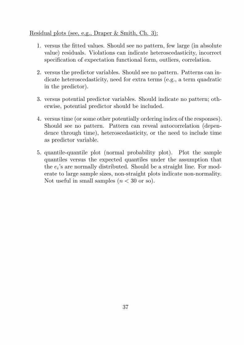
Residual plots (see, e.g., Draper & Smith, Ch. 3):
1. versus the fitted values. Should see no pattern, few large (in absolutevalue) residuals. Violations can indicate heteroscedasticity, incorrectspecification of expectation functional form, outliers, correlation.
2. versus the predictor variables. Should see no pattern. Patterns can in-dicate heteroscedasticity, need for extra terms (e.g., a term quadraticin the predictor).
3. versus potential predictor variables. Should indicate no pattern; oth-erwise, potential predictor should be included.
4. versus time (or some other potentially ordering index of the responses).Should see no pattern. Pattern can reveal autocorrelation (depen-dence through time), heteroscedasticity, or the need to include timeas predictor variable.
5. quantile-quantile plot (normal probability plot). Plot the samplequantiles versus the expected quantiles under the assumption thatthe ei’s are normally distributed. Should be a straight line. For mod-erate to large sample sizes, non-straight plots indicate non-normality.Not useful in small samples (n < 30 or so).
37

Example — Scottish Hill Races Data:
The S-PLUS library MASS contains a data set containing record fastesttimes in 35 Scottish hill races (running races) against distance and totalheight climbed in the race.
• See handout, hills1. This handout contains hills1.SSC, a file contain-ing S-PLUS commands to analyze these data; the associated output;and associated graphics from the analysis.
• On line 2 of hills1.SSC we print out the data. The par(mfrow=c(2,2))command sets up 8 plots per page in a 2×2 grid. In the first plot (la-belled “(a)”) we simply plot time vs. dist. As we should expect, thereappears to be an increasing relationship between time and distance.
• We first fit a simple linear regression model of the form
timei = β0 + β1disti + ei, i = 1, . . . , 35. (m1)
and add the fitted regression line to plot (a). This model appears tofit reasonably well, but we should check residuals.
38

• The functions fitted() and stdres() extract the fitted values and stu-dentized residuals (as I’ve defined them) from the fitted model. Weplot these residuals vs. fitteds in plot (b). Notice that there appearto be several outliers and, perhaps, some increasing variance. In ad-dition, the residuals don’t appear to be centered around zero as muchas would be desirable. This is probably an effect of fitting outliers.
• Next we consider plot (c), a plot of residuals vs. the potential pre-dictor, climb. There appears to be an increasing pattern, suggestingthat climb belongs in the model.
• So, next we fit model m2hills.lm which is of the form
timei = β0 + β1disti + β2climbi + ei, i = 1, . . . , 35. (m2)
• These models are examples of nested models. Note that m1hills.lmis nested in model m2hills.lm in the sense that m1 is a special case ofm2 that occurs when β2 is fixed at 0. We can test m1 versus m2 bytesting H0 : β2 = 0 versus H1 : β2 = 0 in model m2. Notice that thistesting situation is a special case of that described on bottom of p.23with
Aβ − b = ( 0 0 1 )
β0β1β2
− 0.
39

• In nested models testing situations such as this, the F test statisticon the bottom of p.23 has an algebraically equivalent, and more con-venient, form in terms of the degrees of freedom and sums of squaresfor error for the two models:
F =(SSE0 − SSE)/(dfE0 − dfE)
SSE/dfE
where SSE0 and SSE are the sums of squares for error associated withthe null model (model in which H0 holds) and the alternative models,respectively, and dfE0 and dfE are the degrees of freedom for thesetwo models.
– In general, the SSE and dfE for a (full rank) model with p × 1regression parameter β are given by
SSE = ∥y − y∥2 =
n∑i=1
(yi − xTi β︸︷︷︸=yi
)2, dfE = n− p.
– We rejectH0 at significance level α if F > F1−α(dfE0−dfE,dfE).
• The anova() function in S-PLUS automates the testing of nested mod-els using the test described above. It takes as arguments, two fittedmodel objects and tests the null hypothesis that the smaller (null)model holds versus the alternative that it does not under the main-tained hypothesis that the larger model holds. In the example, wereject H0 : {model m1 holds} in favor of model m2 (F = 29.02,p < .0001).
• After adding climb to our model, we recheck the residuals versus climbplot (plot (d)). There still appears to be a pattern to this plot, al-though now it looks different — a convex curve. This suggestes addinga climb2 term.
40

• In m3hills.lm we fit
timei = β0+β1disti+β2climbi+β3climb2i +ei, i = 1, . . . , 35. (m3)
Again, using the anova() function, we see that m3 fits significantlybetter than m2.
• However, the residuals versus climb plot (plot (e)) and the residualsversus fitteds plot (plot (f)) still don’t look particularly good. In plot(f) we can identify the outlier using the identify() function. Type?identify in S-PLUS to get a description on this function.
• We print out the predicted (based on model m3) and observed datafor this outlier using the predict function. Notice that the predictedand observed times are about an hour apart. It is possible that thisdata point was misrecorded. We complete the analysis under thisassumption, omitting this point from further models.
• Model m4hills.lm refits m3 with the outlier removed. Plot (g) displaysthe residuals versus fitteds from this model. These residuals look fairlygood.
• Although there doesn’t appear to be any heteroscedasticity in plot (g),it seems intuitively reasonable that variability in race times shouldincrease with the length of the race. If this were the case, we mightaccount for it be transforming the response so that it had constantvariance on the transformed scale.
• Alternatively, we might consider a model such as m5hills.lm. Thismodel is identical to m4, but instead of the constant variance as-sumption var(ei) = σ2, i = 1, . . . , n, we assume the error variance isproportional to race length squared: var(ei) = σ2dist2i (i.e., the errorstandard deviation is proportional to dist).
• This is an example of a linear model fit withweighted least squares.
41
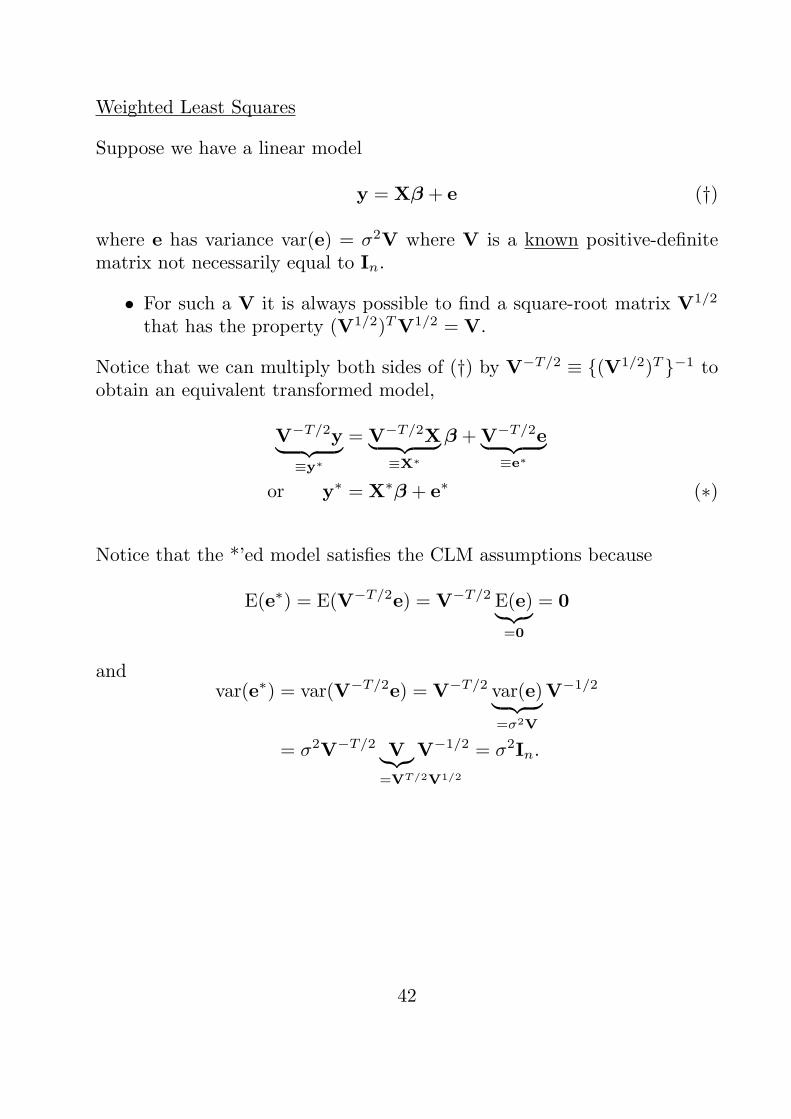
Weighted Least Squares
Suppose we have a linear model
y = Xβ + e (†)
where e has variance var(e) = σ2V where V is a known positive-definitematrix not necessarily equal to In.
• For such a V it is always possible to find a square-root matrix V1/2
that has the property (V1/2)TV1/2 = V.
Notice that we can multiply both sides of (†) by V−T/2 ≡ {(V1/2)T }−1 toobtain an equivalent transformed model,
V−T/2y︸ ︷︷ ︸≡y∗
= V−T/2X︸ ︷︷ ︸≡X∗
β +V−T/2e︸ ︷︷ ︸≡e∗
or y∗ = X∗β + e∗ (∗)
Notice that the *’ed model satisfies the CLM assumptions because
E(e∗) = E(V−T/2e) = V−T/2 E(e)︸︷︷︸=0
= 0
andvar(e∗) = var(V−T/2e) = V−T/2 var(e)︸ ︷︷ ︸
=σ2V
V−1/2
= σ2V−T/2 V︸︷︷︸=VT/2V1/2
V−1/2 = σ2In.
42

Therefore, the (ordinary) least squares estimator of β in (*),
β = {(X∗)TX∗}−1(X∗)Ty∗
= {(V−T/2X)TV−T/2X}−1(V−T/2X)T V−T/2y
= (XTV−1X)−1XTV−1y
is the optimal (BLUE) estimator of β.
• Because this estimator differs from the ordinary least squares esti-mator (XTX)−1XTy by the inclusion of a weight matrix V−1 in theformula, we call this estimator the weighted least squares estima-tor of β.
• It can be shown that the WLS estimator β minimizes
(y −Xβ)TV−1(y −Xβ) (WLS Criterion)
instead of the OLS criterion ∥y −Xβ∥2 = (y −Xβ)T In(y −Xβ).
– This is to say that the OLS estimator minimizes the lengthof y − Xβ with respect to Euclidean distance and the WLSestimator minimizes the length of y − Xβ with respect to amore general statistical distance metric.
– The statistical distance used in WLS is weighted Euclidean dis-tance or Karl Pearson distance in the case that V is a diagonalmatrix. In this case, we are just accounting for heteroscedastic-ity.
– The statistical distance used in WLS is Mahalanobis distancein the case that V is non-diagonal (a.k.a. generalized leastsquares). In this case, we are accounting for heteroscedastic-ity and correlation among the ei’s.
• It’s also straight-forward to show that the WLS estimator β max-imizes the log-likelihood of model (†) under the assumption e ∼Nn(0, σ
2V) so that WLS estimation = ML estimation in this model.
43

Back to the Scottish Hills Races Example:
• In model m5hills.lm, we use the weight option in function lm() to fitthe model using WLS.
• The residuals from this model (plot (h)) don’t look any better thanthose from model m4. It is not possible to test m4 versus m5 usingan F test for nested models (e.g., using the anova() function) becausethese are not nested models. They have the same linear predictor andsame total number of parameters.
• However, it is possible to informally compare the two models usinginformation criteria. Two of the most popular information cri-teria are AIC (Akaike’s Information Criterion) and BIC (BayesianInformation Criterion, a.k.a. Schwarz’s Bayesian Criterion).
• Both of these quantities are penalized version of the maximized log-likelihood function. That is, they measure how likely the data areaccording to the model (as quantified by the loglikelihood functionevaluated at the MLEs of the model parameters) but then penalizethis quantity by an amount related to the complexity of the model.(This same penalization for lack of parsimony idea is the idea behindadjusted R2.)
• For a model with k× 1 parameter vector θ (including all parameters,not just regresison parameters) AIC and BIC are defined as
AIC = −2ℓ(θ;y) + 2k
BIC = −2ℓ(θ;y) + k log(n)
where θ is the MLE of θ.
– AIC and BIC are sometimes given in other forms, but in thisform, the model with the smallest value of AIC (or BIC, if thatcriterion is used) is the winner.
– Its hard to say which criterion is best, but BIC tends to lead tomore parsimonious models than AIC.
44

• The S-PLUS function AIC() and BIC() extract these information cri-teria from fitted model objects. The function logLik() can be used toobtain the maximized log likelihood values.
• According to both AIC and BIC, m4 is preferred to m5, and we aban-don the idea of accounting for heteroscedasticity in this example.
• Although m4 fits pretty well, it is possible to obtain a more parsimo-nious model for these data that fits even better. Venables and Ripley(1999, Ch. 6) consider regressing inverse speed (time/distance) onthe race course gradient (climb/distance). We fit this model,
speed−1i = β0 + β1gradi + ei, i = 1, . . . , n, (m6)
as model m6hills.lm.
• The residuals versus fitted values for m6 (see plot (i)) look as good orbetter than any previous model.
• We produce a Q-Q plot for model m6 using the qqnorm() and qqline()function. This plot (plot (j)) indicates there are more extreme valuesin the data set than expected according to a normal distribution. Thissuggests that a more appropriate distribution for the errors in model(m6) might be a distribution with fatter tails than the normal (e.g.,the t(ν)-distribution with ν small). See Venables and Ripley (1999,Ch.6) for discussion of such a robust regression approach to analyzingthese data.
• The Scottish hill race data are also analyzed in Ch.6 of Maindonald& Braun’s book, Data Analysis and Graphics Using R, which wasdistributed in class.
45

Nonlinear Regression (Ch.2 of Bates & Watts)
We assume that we observe data: (y1,x1), . . . , (yn,xn) where yi is a scalarresponse variable and xi is an m× 1 vector of explanatory variables.
Model:yi = f(xi,θ) + ei, i = 1, . . . , n,
where e1, . . . , eniid∼ N(0, σ2)
where
f(·) is a known function (the expectation or regression function)
θ is a p× 1 parameter vector
ei’s are i.i.d. error terms
f(·) is a nonlinear function of θ. That is,
∂f(x,θ)
∂θjdepends on θ for some j.
• If f(·) is nonlinear in any component of θ, it is a nonlinear model.
Let ηi(θ) = f(xi,θ) and η = (η1, . . . , ηn)T . Then we can write our model
equivalently asy = η(θ) + e, e ∼ Nn(0, σ
2In).
Some examples of expectation functions:
f(x,θ) =θ1x
θ2 + x(Michaelis-Menten Model)
f(x,θ) =θ1
1 + exp{(θ2 − x)/θ3}(Simple Logistic Model)
f(x,θ) = θ1 + (θ2 − θ1) exp{− exp(θ3)x} (Asymptotic Regression Model)
f(x,θ) = θ1 + θ2x1 + θ3xθ42 (regression w/ power trans. of x2)
46

How do we choose f(·)?
1. Mechanistic models. Often there is some scientific theory availablethat describes the data-generating mechanism. This theory suggeststhe form of f .
2. Empirical models. At other times no theory is available or we simplywant to describe the relationship between y and x in a simple modelor develop a model that produces good predictions (unconcerned byhow those predictions come about). In such cases we simply try to“fit the data”. For data that follow certain general shapes of curves(e.g., sigmoidal, parabolic, etc.) “promising candidates” for nonlinearexpectation functions are available (e.g., Ratkowsky, 1990) that canbe tried.
• In linear modelling, empirical models are most common. In nonlinearmodelling, mechanistic models are more common.
Example — Wind Speed:
Consider the following five measurements of wind speed (y, in cm/sec) atvarious heights (x in cm):
x y
40 490.280 585.3160 673.7320 759.2640 837.5
47

These data are plotted below
•
•
•
•
•
Height (cm)
Win
d S
peed
(cm
/sec
)
100 200 300 400 500 600
500
600
700
800
• See handout, “wind1”.
• For these data we might consider fitting linear models.
Model 1 (simple linear regression):
yi = β0 + β1xi + ei, i = 1, . . . , 5
yields R2 = 0.847, and residual standard deviation s =√mse = 62.13.
Model 2 (quadratic regression):
yi = β0 + β1xi + β2x2i + ei, i = 1, . . . , 5
yields R2 = 0.975, and residual standard deviation s =√mse = 30.52.
48

• The fitted regression lines for these models are plotted on the lastpage of wind1. Clearly, model 1 is inadequate. Model 2 fits ok, butnot great. We’ve already used 3 out of 5 d.f. to fit this model, sogoing to a cubic to improve the fit is not particularly attractive.
Theory: Under adiabatic conditions, wind speed is related to height as
windspeed = θ1 log{height(1− θ2/θ3)− 1/θ3}, (∗)
whereθ1 = friction velocity
θ2 = zero point displacement
θ3 = roughness length
This relationship is not likely to hold exactly for our data due to mea-surement error and deviations from the ideal conditions under which therelationship is theorized to hold. Therefore, we fit a stochastic version of(*):
yi = θ1 log{xi(1− θ2/θ3)− 1/θ3}+ ei, i = 1, . . . , 5. (∗∗)
• Notice the model (**) is nonlinear since ∂f(x,θ)/(∂θj) depends uponθ for all j = 1, 2, 3. E.g.,
∂f(x,θ)
∂θ1= log{xi(1− θ2/θ3)− 1/θ3}.
• For now, we skip the details of how to fit a nonlinear such as (**),but in R it can be done using nonlinear least squares with the nls()function. The parameter estimates (standard errors) turn out to be
θ1 = 115.1(2.04), θ2 = −.0595(.00546), θ3 = .0454(.0132).
49

• The fitted regression line for model (**) fits the observed data muchmore closely than that of either linear model. In addition, the residualstandard deviation of the nonlinear model, s = 1.87, is much smallerthan for the linear models.
• Perhaps most importantly, this model reflects what is know aboutthe relationship between wind speed and the height at which it ismeasured, and the parameter estimates have specific, useful interpre-tations in terms of the physics/meteorology of the problem.
Classes of Nonlinear Models:
1. Yield-Density Models.
– Common in agriculture (e.g., forestry).
– Models describe the relationship between the yield of a crop andthe density of planting.
LetX = plant density in plants/unit area
R = yield/plant.
ThenW = XR = total yield per unit area (e.g., acre).
Two common yield density relationships:
i. “asymptotic relationship” (most crops. e.g., carrots, beans, tomatoes)
50

ii. “parabolic relationship” (e.g., sweet corn, cotton)
A common model for the asymptotic case is
R = (θ1 + θ2X)−1.
Notice that as X → 0, R → 1/θ1 ⇒ θ−11 has interpretation as the
“genetic potential” of a crop uninhibited by competition. In addition,as X → ∞, W = XR→ 1/θ2, ⇒ θ−1
2 =“environmental potential”.
For observed data, the model
Ri = (θ1 + θ2Xi)−1 exp(ei)
is often used; or, transforming,
Yi = log(θ1 + θ2Xi) + ei,
where Yi = − log(Ri).
– This model is not based on any theory, its simply an empiricalmodel whose parameters have meaningful interpretations in thiscontext.
51

An important model that is used in the asymptotic case of the yield-density curve but also in a wide variety of other applications is theAsymptotic Regression Model:
Yi = α− βγXi + ei, i = 1, . . . , n.
This model yields a curve that has the following shape:
• As with many named classes of nonlinear models, a variety of differentparameterizations of the asymptotic regression models are used:
Yi = θ1 − θ2e−θ3Xi + ei, (here, e−θ3 = γ)
Yi = θ1 − θ1e−(Xi+θ2)θ3 + ei,
Yi = θ1 − e−(θ2+θ3Xi) + ei
• In nonlinear regression, the parameterization you use affects the al-gorithms used to solve the models, the properties of the estimators,and the accuracy of approximations used for inference. To a muchgreater degree than in linear models, it is important to choose theright parameterization! We will return to this point later.
52

2. Growth Models.
– These models relate the size or change in size of some entity totime.
The most common shape for growth curves is a “sigmoidal curve”:
Let R =a measure of size, and X =time. There are several com-monly used growth curves that capture the sigmoidal shape for R asa function of X; e.g.,
R = θ1 exp{− exp(θ2 − θ3X)}, (Gompertz)
R =θ1
1 + exp(θ2 − θ3X), (simple logistic)
R =θ1X
θ2 + θ3θ4Xθ2 + θ3
, (Morgan-Mercer-Flodin)
R = θ1{1− exp(−θ2X)}θ3 , (Chapman-Richards)
• In fitting these models to data, either an additive or multiplicativeerror term may be appropriate. E.g., in the case of the logistic modelwe might consider an additive version:
Yi =θ1
1 + exp(θ2 − θ3Xi)+ ei, where Yi = Ri
or a multiplicative version:
Yi = log(θ1)− log{1 + exp(θ2 − θ3Xi)}+ ei, where Yi = log(Ri).
53

3. Compartmental Models and Other Models Based on Systems of Dif-ferential Equations.
– Compartmental models are mechanistic models where one ormore measurements of some physical process is related to time,inputs to the system, and other explanatory variables througha compartmental system.
– A compartmental system is “a system which is made up of afinite number of macroscopic subsystems, called compartmentsor pools, each of which is homogeneous and well mixed, and thecompartments interact by exchanging materials. There may beinputs from the environment into one or more of the compart-ments, and there may be outputs (excretion) from one or morethe compartments to the environment.” (Seber & Wild, p.367)
– Compartmental models are common in chemical kinetics, toxi-cology, hydrology, geology, and pharmacokinetics.
As an example from pharmacokinetics, consider the data in the fol-lowing scatterplot on tetracycline concentration over time.
•
•
• •
•
•
•
•
•
Time (hrs)
Tet
racy
clin
e C
once
ntra
tion
(mug
/ml)
5 10 15
0.4
0.6
0.8
1.0
1.2
1.4
Tetracycline Concentration vs. Time
54

The data come from a study in which a tetracycline compound wasadministered to a subject orally, and the concentration of tetracyclinehydrochloride in the blood serum was measured over a period of 16hours (the data are in Appendix A1.14 of Bates & Watts).
A simple compartmental model for the biological system determiningtetracycline concentration in serum is one that hypothesizes
a. a gut compartment into which the chemical is introduced,
b. a blood compartment which absorbs the chemicals from the gut,and
c. an elimination path.
This simple two-compartment open model can be represented in acompartment diagram as follows:
Here, γ1 and γ2 represent the the concentrations of the chemical incompartments 1 and 2, respectively, and θ1 and θ2 represents rates oftransfer into and out of compartment 2, respectively.
55

Under the assumption of first-order (linear) kinetics, it is assumedthat at time t, the rate of elimination from any compartment is pro-portional to γ(t), the concentration currently in that compartment.
Thus the rates of change in the concentrations in the two compart-ments in the model represented above are
∂γ1(t)
∂t= −θ1γ1(t)
∂γ2(t)
∂t= θ1γ1(t)− θ2γ2(t)
Differential equations solutions for linear compartmental models gen-erally take the form of linear combinations of exponentials. Therefore,these models are nonlinear models that can be fit using methods sim-ilar to those used for yield-density models, growth curve models, etc.
For example, the solution for γ2(t), the concentration in blood serumat time t is
γ2(t) =θ3θ1(e
−θ1t − e−θ2t)
θ2 − θ1.
• Here, θ3 is the amount of drug (tetracycline) ingested initially (attime t = 0).
56

Therefore, we might try the additive error model
yi =θ3θ1(e
−θ1ti − e−θ2ti)
θ2 − θ1+ ei, i = 1, . . . , n,
to model the tetracycline data. The resulting fitted regression curveis displayed below.
•
•
• •
•
•
•
•
•
Time (hrs)
Tet
racy
clin
e C
once
ntra
tion
(mug
/ml)
5 10 15
0.4
0.6
0.8
1.0
1.2
1.4
Tetracycline Concentration vs. Time
4. Multiphase and Spline Regressions.
In multiphase and spline regression models, the expectation functionfor the regression of y on x, E(y) = f(x;θ), is obtained by piecingtogether different curves over different intervals.
57

That is, in multiphase and spline models,
f(x;θ,α) =
f1(x;θ1), x ≤ α1;f2(x;θ2), α1 < x ≤ α2;...
...fD(x;θD), αD−1 < x.
– Here, the expectation function f(x;θ,α) is defined by differentfunctions (f1, f2, . . . , fD) on different intervals, and typically theendpoints of the intervals are unknown and must be estimated.
– The D submodels are referred to as phases, and the α’s arechangepoints.
– Multiphase models are intended for situations in which (a) thenumber of phases is small; (b) the behavior in each phase iswell-described by a simple parametric function like a line orquadratic; and (c) there are fairly abrupt changes between regimes.
– Spline models have the same piecewise form, but the individualphase models fd, d = 1, . . . , D, are always polynomials and theemphasis is on joining these “splines” to obtain a smooth andvery flexible function to capture the underlying regression form.
• After presenting methodology for the general nonlinear regressionmodel, we’ll come back and spend some more time on certain spe-cial class of nonlinear models as time allows.
58

Special Types of Nonlinear Models:
1. Transformably Linear Models:
Suppose we observe zi, xi, i = 1, . . . , n, where
E(zi) = f(xi;θ).
If it is possible to find a transformation h(·) such that yi = h(zi)satisfies a linear regression model, then we say that the expectationfunction f is transformably linear.
• We must be careful about assumptions on error terms when usinglinearizing transformations!
SupposeE(zi) = eα+βxi .
If the error in zi is proportional to the expected magnitude of zi butotherwise independent of xi (“constant relative error”) then we canwrite a model for zi as
zi = eα+βxi(1 + ei),
where
E(ei) = 0, and var(ei) = σ2 (constant variance).
Equivalently,zi = eα+βxi + e∗i (∗)
where e∗i = E(zi)ei has mean 0 and variance var(e∗i ) = σ2{E(zi)}2.
If we transform to linearity by taking logs we get
yi = α+ βxi + log(1 + ei), where yi = log(zi)
= α+ βxi + ei,
where ei = log(1+ ei) has mean E(ei) ≈ E(ei) = 0 (for small ei), andvariance var(ei) that is independent of xi.
59
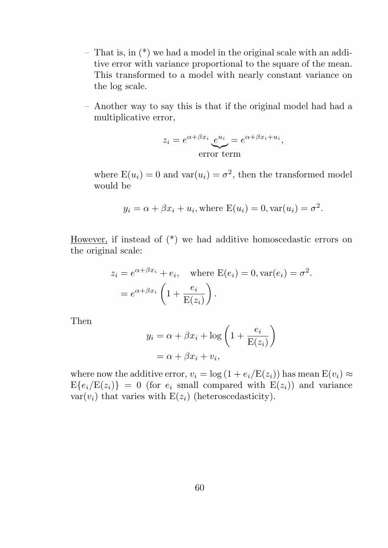
– That is, in (*) we had a model in the original scale with an addi-tive error with variance proportional to the square of the mean.This transformed to a model with nearly constant variance onthe log scale.
– Another way to say this is that if the original model had had amultiplicative error,
zi = eα+βxi eui︸︷︷︸error term
= eα+βxi+ui ,
where E(ui) = 0 and var(ui) = σ2, then the transformed modelwould be
yi = α+ βxi + ui,where E(ui) = 0, var(ui) = σ2.
However, if instead of (*) we had additive homoscedastic errors onthe original scale:
zi = eα+βxi + ei, where E(ei) = 0, var(ei) = σ2.
= eα+βxi
(1 +
eiE(zi)
).
Then
yi = α+ βxi + log
(1 +
eiE(zi)
)= α+ βxi + vi,
where now the additive error, vi = log (1 + ei/E(zi)) has mean E(vi) ≈E{ei/E(zi)} = 0 (for ei small compared with E(zi)) and variancevar(vi) that varies with E(zi) (heteroscedasticity).
60

To summarize:
– homoscedasticity on original scale generally induces heteroscedas-ticity on transformed scale. In this case, we should either fit ahomoscedastic nonlinear model to the original data (NLS) or useWLS to fit a heteroscedastic linear model on the transformedscale.
– Certain types of heteroscedasticity on the original scale can leadto homoscedasticity on the transformed scale. In this case, ei-ther nonlinear WLS on the original scale or linear OLS on thetransfored scale can be used.
– As long as the error variance is accounted for correctly, work-ing on either the linear or nonlinear scale may be appropriate.Desirability of interpretable parameter estimates may argue fornonlinear model on original scale.
– We assume nonlinear model will be fit. Even in this case avail-ability of a linear transformation can be very useful (e.g., forobtaining starting values).
– Note that transformations affect entire distribution of the errorterms, not just their variance. ⇒ normal additive errors on orig-inal scale lead to non-normal additive errors on the transformedscale.
2. Partially Linear Models:
Consideryi = θ1(1− e−θ2xi) + ei.
If θ2 is known (i.e., fixed) then the model is linear:
yi = θ1wi + ei, where wi = 1− e−θ2xi .
61

θ1 is a conditionally linear parameter if for fixed θ2, . . . , θp themodel is linear.
If there is at least one conditionally linear parameter in the modelthen the model is partially linear.
– For partially linear models, some procedures (e.g., obtainingstarting values) are simplified.
Geometry of the Expectation Surface:
Consider the linear model with n = 2, p = 1 and model equation
yi = θxi + ei, i = 1, 2
where x1 = 1, x2 = 2.
The expectation plane is the set of all 2×1 vectors η(θ) = θ
(12
). We plot
this expectation plane below
62

Features:
1. Linearity (with respect to θ).
a. The effect of changing θ by δ units is the same for all θ.
b. θ points with equal spacing correspond to η points with equalspacing.
c. Line segments in the parameter space correspond to line seg-ments in the expectation plane.
– (a)–(c) above are all essentially restatements of the same idea,linearity.
2. Expectation is of infinite extent.
Now consider the nonlinear model:
yi =1
1 + e−θxi+ ei. (∗)
Again, take x = (x1, x2)T = (1, 2)T . Then the expectation surface is
η(θ) =
((1 + e−θ)−1
(1 + e−2θ)−1
), (1-dim. surface in 2-space)
63

We can plot this surface in 2-space by plugging a few values of θ into the
formula for η(θ) =
(η1(θ)η2(θ)
):
θ η1 η2
−∞ 0 0−2 .119 .0180−1 .269 .1190 .500 .5001 .731 .8812 .881 .982∞ 1 1
eta1
eta2
0.0 0.5 1.0
-0.2
0.0
0.2
0.4
0.6
0.8
1.0
1.2
theta=-inftytheta=-2
theta=-1
theta=0
theta=1
theta=2theta=infty
Expectation Surface for Example Nonlinear Model
64

Features:
1. Nonlinearity:
a. Effect of changing θ by 1 unit depends upon the value of θ.
b. θ points with equal spacing correspond to η points with unequalspacing.
c. Line segments in the parameter space correspond to curves inthe expectation space.
2. The expectation surface may be of finite extent.
• The curved shape of the expectation surface is invariant to reparam-eterization. That is, the degree of curvature is the same no matterwhat parameterization is used. This aspect of nonlinearity is knownas intrinsic nonlinearity.
• The extent to which equally-spaced θ points map to unequally spacedη-points is known a parameter-effects nonlinearity. This type ofnonlinearity depends upon the parameterization chosen for the model.A good parameterization leads to small parameter-effects nonlinearity.
For example, consider the following reparameterization of model (*) on p.63:
yi =1
1 + ϕ−xi+ ei, here, ϕ = eθ.
65

We can again plot the expectation surface based on the new parameteriza-tion. The result is as follows:
eta1
eta2
-5 0 5 10
0.0
0.2
0.4
0.6
0.8
1.0
phi parameterization, entire expect. surface
eta1
eta2
0.0 0.5 1.0
-0.2
0.0
0.2
0.4
0.6
0.8
1.0
1.2
phi parameterization, phi>=0
phi=0
phi=1
phi=2
phi=3phi=4
phi=10 phi=1e10
• Notice that under the reparameterization, the expectation surface isof infinite extent.
• Restricting attention to the region ϕ ≥ 0 (corresponding to the en-tire range of θ) depicted in the right-hand plot, we see that theθ-parameterization has the exact same intrinsic nonlinearity as theϕ−parameterization.
• However, the θ-parameterization has considerably less parameter-effectsnonlinearity than the ϕ-parameterization. This is so because underthe ϕ-parameterization, η-curve segments corresponding to values ofϕ one unit apart differ in length to a much greater extent than underthe θ-parameterization.
66

• Note that the degree of both intrinsic nonlinearity and parameter-effects nonlinearity in a particular model depend upon the values ofx. Two models with the same form and parameterization but differentvalues of the explanatory variables will have different nonlinearitiesof both types.
E.g., if we change x from (1, 2)T to (−1, 5)T we get the following curves.
eta1
eta2
0.0 0.5 1.0
-0.2
0.0
0.2
0.4
0.6
0.8
1.0
1.2
theta parameterization. x=(1,5)
theta=-infty theta=-2theta=-1
theta=0
theta=1theta=2
theta=infty
eta1
eta2
0.0 0.5 1.0
-0.2
0.0
0.2
0.4
0.6
0.8
1.0
1.2
phi parameterization. x=(1,5)
phi=0
phi=1
phi=2
phi=3 phi=4
phi=1e10
• Later in the course we will come back to the ideas of intrinsic andparameter-effects nonlinearity and discuss measures of these two-typesof curvature. For now, suffice it to say that it is desirable to chooseparameterizations with low parameter-effects nonlinearity.
67

Linear Approximations:
Let h(·) denote a (twice differentiable) scalar valued function of a scalarargument. For any fixed points u and u∗, Taylor’s Theorem says
h(u) = h(u∗) + h′(u∗)(u− u∗) +1
2h′′(u∗∗)(u− u∗)2,
where h′(u∗) = ∂h(u)∂u
∣∣u=u∗ , h
′′(u∗∗) = ∂2h(u)∂u2
∣∣u=u∗∗ , and u∗∗ is a point
between u and u∗.
If u∗ is close to u, then the last term in this expansion will be small relativeto the rest and we have
h(u) ≈ h(u∗) + h′(u∗)(u− u∗) ≡ h(u)
for u close to u∗.
• This is known as a first-order (linear) Taylor series approxima-tion.
This approximation is
i. Linear. (h(u) is a linear function of u.)
ii. Local. (Only valid for u near u∗.)
Now suppose h is a scalar-valued function of u, a p × 1 vector. For thissituation the above linear Taylor series approximation generalizes to
h(u) ≈ h(u∗) +∂h(u∗)
∂uT︸ ︷︷ ︸1×p
(u− u∗)︸ ︷︷ ︸p×1
for u close to u∗ (that is, when ∥u− u∗∥ is small).
Here,
u =
u1...up
,u∗ =
u∗1...u∗p
, and∂h(u∗)
∂uT=
(∂h(u)∂u1
∂h(u)∂u2
· · · ∂h(u)∂up
)
68

If we prefer a non-vector notation form, we can multiply out the secondterm and write this approximation in an equivalent form as follows:
h(u) ≈ h(u∗) + (u1 − u∗1)∂h(u)
∂u1
∣∣∣u=u∗
+ · · ·+ (up − u∗p)∂h(u)
∂up
∣∣∣u=u∗
.
Consideryi = f(xi,θ) + ei,
= ηi(θ) + ei,i = 1, . . . , n,
or, in vector form,y = η(θ) + e.
Estimation and inference about θ is easy if f(xi,θ) is linear in θ. Thissuggests using a linear Taylor series approximation of f(xi,θ).
For θ near θ∗,
f(xi,θ) ≈ f(xi,θ∗) + (θ1 − θ∗1)Vi1 + · · ·+ (θp − θ∗p)Vip,
for each i = 1, . . . , n, where
Vij =∂f(xi,θ)
∂θj
∣∣∣θ=θ∗
.
Stacking these n approximations on top of one another in vector form wehave
η(θ) ≈ η(θ∗) +V(θ∗)(θ − θ∗),
where V(θ∗) is the n× p matrix with (i, j)th element Vij . (I.e., V(θ∗) has
ith row ∂f(xi,θ)
∂θT
∣∣θ=θ∗ .)
69

A picture of the Taylor series linear approximation taken at θ∗ = 2:
eta1
eta2
0.0 0.5 1.0
0.0
0.5
1.0
theta=2
Estimation of θ:
Under the assumption that e ∼ Nn(0, σ2In), the MLE of θ is also the
nonlinear least-squares estimator. I.e., it is the value of θ that minimizes
∥y − η(θ)∥2 =
n∑i=1
{yi − f(xi,θ)}2.
• This is still the (ordinary) least squares criterion. The only differenceis that f(xi,θ) = xT
i θ (nonlinearity).
• As in linear least squares, we need to find the point on the expectationsurface, η(θ), that is closest to y in terms of Euclidean distance.
• This is a harder problem because the expectation surface is no longera plane.
70

E.g., Suppose y = (.85, .85)T in our example from p.63–64.
eta1
eta2
0.0 0.5 1.0
-0.2
0.0
0.2
0.4
0.6
0.8
1.0
1.2
y=(.85,.85)’
• In the nonlinear case, finding the point η on the expectation surfaceis hard because of intrinsic nonlinearity.
• Once we find η we must find the value of θ solving η(θ) = η. Inlinear regression this step is easy because the mapping from β to ηis linear and invertible. In nonlinear regression, this step is harder,because of both intrinsic and parameter-effects nonlinearity.
71

Nonlinear least squares: find the θ to minimize
S(θ) = ∥y − η(θ)∥2 =n∑
i=1
{yi − f(xi,θ)}2.
Q: How do we minimize S(θ)?
A: Solve normal equations.
Taking derivatives we get
∂S(θ)
∂θj= −2
n∑i=1
{yi − f(xi,θ)}∂f(xi,θ)
∂θj, j = 1, . . . , p,
or, in matrix notation,
∂S(θ)
∂θT= −2[y − η(θ)]T V(θ)︸ ︷︷ ︸
n× p derivative matrix
Therefore, θ satisfies[y − η(θ)]TV(θ) = 0. (†)
• Recall that in linear regression, the derivative matrix was V(θ) = Xand our normal equation took the form of the orthogonality condition:
[y −Xβ]TX = 0,
which says, the residual vector y−Xβ is orthogonal to the expectationplane (all vectors of the form Xβ).
• In the nonlinear case, (†) says that the residual vector y − η(θ) is
orthogonal to the “tangent plane” to the expectation surface at θ = θ.
72

• Notice (†) is nonlinear in θ and doesn’t, in general, yield a closed form
expressionfor the solution, θ.
Q: How do we solve a nonlinear set of equations like (†)?
A: Usually requires an iterative method. For example,...
Gauss-Newton Method
The G-N method proceeds by
1. Obtaining a starting value θ0.
2. Using a linear approximation to η(θ) for θ near θ0.
3. Using linear regression methods to “estimate θ”; i.e., to update θ0 toθ1.
4. Repeat steps 2 and 3 until convergence.
Let V0 = V(θ0). Then,
η(θ) ≈ η(θ0) +V0(θ − θ0)
for θ near θ0. It follows that
y − η(θ) ≈ y − η(θ0)︸ ︷︷ ︸≡z0
−V0 (θ − θ0)︸ ︷︷ ︸≡δ
≡ z0 −V0δ
Therefore, for θ near θ0, choosing θ to minimize ∥y − η(θ)∥2 is “approxi-mately equivalent to” (should give nearly the same result as) the problemof choosing δ to minimize ∥z0 −V0δ∥2.
• This minimization can be carried out using linear regression. E.g., wecould use δ = {(V0)TV0}−1(V0)T z0. However, this formula, whilecorrect, is not the best way to do the computations - either here, orin regular linear regression.
73

This process consists of two steps:
a. Obtaining the point η∗ = V0δ.
b. Determining δ from η∗.
Once we have δ, we can easily translate to θ. From its definition,
δ = θ − θ0 θ = θ0 + δ.
Therefore, we can update θ0 to θ1 via
θ1 = θ0 + δ (∗)
• Because of this updating formula, we call δ the Gauss-Newton in-crement.
• θ is updated this way until convergence.
Complication: There is no guarantee that the update will reduce the ob-jective function S(θ). I.e., no guarantee that S(θ1) < S(θ0).
We can fix this problem simply enough. If S(θ1) ≥ S(θ0) then replace theupdate (*) by
θ1 = θ0 + λδ, where 0 < λ ≤ 1.
To choose λ, start with λ = 1 and then try λ values 1, 12 ,14 ,
18 , . . . until we
find a λ value that gives S(θ1) < S(θ0).
• λ is called a step factor.
74

Each of the steps a and b in the description of the G-N algorithm above ismade easier by using the QR Decomposition
The QR Decomposition:
• Our interest right now is in using the QR decomposition in the non-linear model, but just to keep things simple, let’s return to the linearmodel for a moment.
In the linear model, the least squares problem is to find the value of β tominimize
∥y −Xβ∥2
We know that (if XTX is invertible) the answer is
β = (XTX)−1XTy
.
• However, the computation of β via this formula can be computa-tionally inefficient and error-prone. A better way is with the QRdecomposition.
In general, an n× p (n ≥ p) matrix X can be decomposed as
X = QR
where Q is an n × n orthogonal matrix (it has the property QQT =QTQ = In) and R is a n× p matrix of the form
R =
(R1
0
)whereR1 is a p×p upper-triangular matrix (it has zeros below the diagonal).
• From the fact that the last n− p rows of R contain 0’s we can write
X = QR = (Q1︸︷︷︸n×p
, Q2︸︷︷︸n×(n−p)
)
(R1
0
)= Q1R1
75

where Q1 consists of the first p columns of Q and R1 contains thefirst p rows of R.
Since we know that β = (XTX)−1XTy, it also follows that the mean of y,Xβ has least squares estimate
Xβ = X(XTX)−1XTy
Applying the QR decomposition to X we get
Xβ = Q1R1(RT1 QT
1 Q1︸ ︷︷ ︸=I
R1)−1RT
1 QT1 y
= Q1R1(R1)−1(RT
1 )−1RT
1 QT1 y
= Q1QT1 y
= Q
(QT
1 y0
)= Q
(w1
0
)where w1 = Q1y.
• So, we have that
Xβ = Q
(w1
0
)(♣)
which allows us to get the least squares estimate of the mean of ywithout computing a matrix inverse - a computationally demandingan error-prone task.
76

All that’s left to do is find β once we haveXβ. This is easy because applyingthe QR decomposition to X again in (♣), we get
Xβ = Q
(w1
0
)⇒ QRβ = Q
(w1
0
)⇒ QTQ︸ ︷︷ ︸
=I
Rβ = QTQ︸ ︷︷ ︸=I
(w1
0
)
⇒ Rβ =
(w1
0
)⇒ R1β = w1 (♢)
• Solving for β is now easy because R1 is upper-triangular!
E.g., suppose that in a simple linear regression problem we did the compu-
tations and found that w1 =
(2−1
)and R1 =
(1 11
30 1
3
)then to obtain β
we would solve (1 11
30 1
3
)(β1β2
)=
(2−1
)
⇒β1 +
11
3β2 = 2
1
3β2 = −1
which solve easily to give
β2 = −3, β1 = 13.
77

Back to the G-N method for the nonlinear model:
Steps a and b above were aimed at finding the G-N increment δ by mini-mizing ∥z0 −V0δ∥2. The steps were:
a. Obtaining the point η∗ = V0δ.
b. Determining δ from η∗.
By utilizing the QR-decomposition V0 = QR = Q1R1 in step a, we obtainthe computationally efficient formula :
η∗ = Q1QT1 z
0. (compare p.76)
(Note that η∗ lies on the tangent plane to the expectation surface, it’s noton the expectation surface itself - hence the star notation. I.e., η∗ isn’tequal to η(θ) for any θ.)
Then in step b, δ can be determined from η∗ by solving the linear equation,η∗ = V0δ. Or, since we can write this equation asQ1R1δ = η∗ = Q1Q
T1 z
0,this step reduces to solving
R1δ = QT1 z
0, (compare (♢))
which is easy because R1 is upper triangular.
78
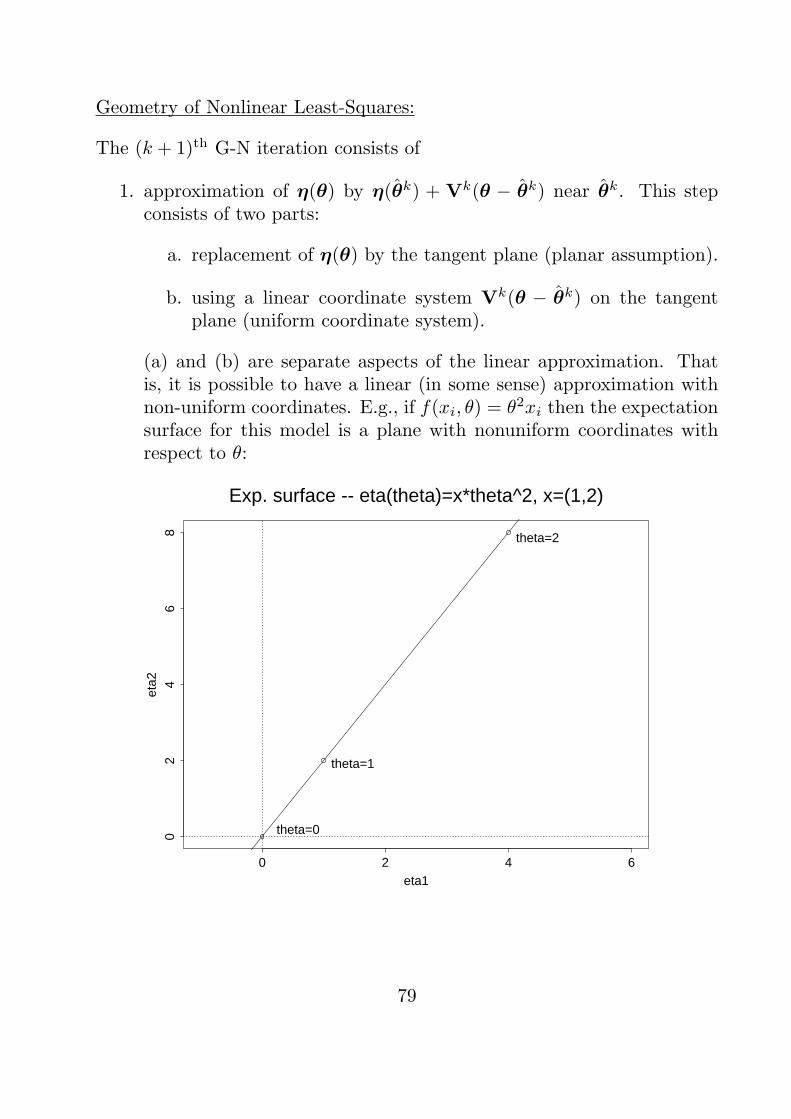
Geometry of Nonlinear Least-Squares:
The (k + 1)th G-N iteration consists of
1. approximation of η(θ) by η(θk) + Vk(θ − θk) near θk. This stepconsists of two parts:
a. replacement of η(θ) by the tangent plane (planar assumption).
b. using a linear coordinate system Vk(θ − θk) on the tangentplane (uniform coordinate system).
(a) and (b) are separate aspects of the linear approximation. Thatis, it is possible to have a linear (in some sense) approximation withnon-uniform coordinates. E.g., if f(xi, θ) = θ2xi then the expectationsurface for this model is a plane with nonuniform coordinates withrespect to θ:
eta1
eta2
0 2 4 6
02
46
8
theta=0
theta=1
theta=2
Exp. surface -- eta(theta)=x*theta^2, x=(1,2)
79
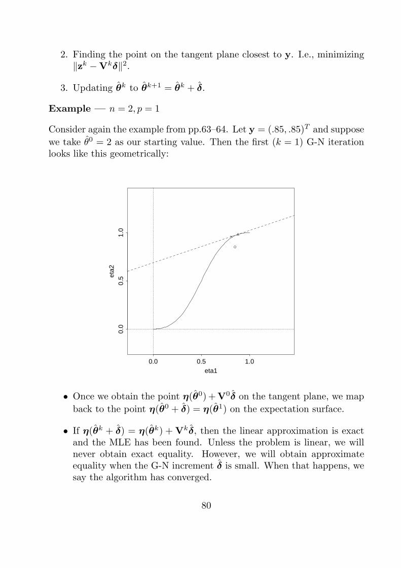
2. Finding the point on the tangent plane closest to y. I.e., minimizing∥zk −Vkδ∥2.
3. Updating θk to θk+1 = θk + δ.
Example — n = 2, p = 1
Consider again the example from pp.63–64. Let y = (.85, .85)T and suppose
we take θ0 = 2 as our starting value. Then the first (k = 1) G-N iterationlooks like this geometrically:
eta1
eta2
0.0 0.5 1.0
0.0
0.5
1.0
• Once we obtain the point η(θ0) +V0δ on the tangent plane, we map
back to the point η(θ0 + δ) = η(θ1) on the expectation surface.
• If η(θk + δ) = η(θk) +Vkδ, then the linear approximation is exactand the MLE has been found. Unless the problem is linear, we willnever obtain exact equality. However, we will obtain approximateequality when the G-N increment δ is small. When that happens, wesay the algorithm has converged.
80

Convergence of the Algorithm:
Let θk denote the estimate from the kth iteration. Convergence can bemeasured in several ways:
1. Look at change in the parameter estimates:
If θk ≈ θk−1 we may consider the sequence θ0, θ1, θ2, . . . to haveconverged and take θ = θk as the MLE/NLS estimator.
The most common way to establish that θk ≈ θk−1 is to look at
maxj
|θkj − θk−1j |
|θk−1j |
.
If this criterion is less than some tolerance value (1 × 10⁻⁶, say) thealgorithm stops.
2. Look at change in the objective function S(θ):
If S(θk) ≈ S(θk−1) then take θ = θk. To judge this we can use thecriterion
S(θk−1)− S(θk)
S(θk).
Again, if this criterion is smaller than some tolerance value, then stop.
Q: Which approach, 1 or 2, is better?
A: It depends. If the main interest is in the mean response, η(θ), then (2)may be more appropriate. If the regression parameters themselves are ofmore interest than perhaps (1) is better.
81

Both criteria have the disadvantage that they don’t indicate when θk isclose to θ or when S(θk) is close to S(θ).
E.g., if we knew the minimum value of the least squares criterion S(θ) wasequal to 10, say, then we could stop the algorithm based on judging whenS(θk) ≈ 10.
Of course, we would never know S(θ) or θ to judge convergeence to the
optimal value in this manner. However, we do know that θ must satisfy thenormal equation
[y − η(θ)]TV(θ) = 0
therefore we can stop iterating when
[y − η(θk)]T︸ ︷︷ ︸residual vector for θk
V(θk) ≈ 0.
This suggests a third convergence criterion:
3. Relative offset criterion. Based on θk, the residual vector [y−η(θk)],can be written as the sum of two components:
– a vector in the tangent plane
– a vector ⊥ to the tangent plane
82

These two components can be seen in the following plot
eta1
eta2
0.0 0.5 1.0
0.0
0.5
1.0
This is to say that [y − η(θk)] can be written as
[y − η(θk)] = ψ1 +ψ2
where ψ1 is in the tangent plane, and ψ2 is ⊥ to the tangent plane.
Then one measure of “how orthogonal” y − η(θk) is to the tangentplane is
∥ψ1∥∥ψ2∥
the relative offset criterion
• When this criterion is close to zero, the ψ1 component of y − η(θk)is negligible, implying y − η(θk) is approximately ⊥ to the tangent
plane; i.e., [y − η(θk)]TV(θk) ≈ 0.
• It can be shown that the components ψ1 and ψ2 have lengths
∥ψ1∥ = ∥QT1 [y − η(θk)]∥, ∥ψ2∥ = ∥QT
2 [y − η(θk)]∥
where Q = [Q1,Q2] is the Q matrix from a QR-decomposition of
V(θk).
83

Inference Using the Linear Approximation:
• The basic approach to inference in nonlinear models is to use the linearapproximation to reduce the situation to the linear case and then usestandard linear models results. Because of the approximation, theseresults will be approximate rather than exact.
Recall that the (nonlinear) least squares estimator θ minimizes
S(θ) = ∥y − η(θ)∥2
Let θ∗ denote the true value of θ. Using the linear Taylor series approxi-mation, we can approximate η(θ) for θ close to θ∗ as
η(θ) ≈ η(θ∗) +V(θ∗)(θ − θ∗)
It follows that
y − η(θ) ≈ y − η(θ∗)︸ ︷︷ ︸≡z∗
−V(θ∗) (θ − θ∗)︸ ︷︷ ︸≡δ∗
= z∗ −V(θ∗)δ∗
so thatS(θ) = ∥y − η(θ)∥2
≈ ∥z∗ −V(θ∗)δ∗∥2 ≡ S∗(θ).
84

We know from linear models that the value of
=δ∗︷ ︸︸ ︷θ − θ∗ that minimizes S∗(θ)
is{(V∗)TV∗}−1(V∗)T z∗,
where V∗ ≡ V(θ∗).
It follows that the value of θ that minimizes S∗(θ) is
{(V∗)TV∗}−1(V∗)T z∗ + θ∗.
It’s also true that the value of θ that minimizes S(θ) is θ.
Therefore, since S(θ) ≈ S∗(θ) in a neighborhood of θ∗ (which we should
expect to contain θ, since θ is a “good estimator”) these two minimizersshould be approximately equal:
θ ≈ {(V∗)TV∗}−1(V∗)T z∗ + θ∗
or, equivalently,
θ ≈ θ∗ + {(V∗)TV∗}−1(V∗)T [y − η(θ∗)]︸ ︷︷ ︸=e
= θ∗ + {(V∗)TV∗}−1(V∗)Te
This result,θ ≈ θ∗ + {(V∗)TV∗}−1(V∗)Te (†)
is an approximate version of the exact result
β = β + (XTX)−1XTe (see p.21)
that we had for the linear model, where the derivative matrix has changedfrom X to V(θ∗).
85

From (†), analogues of all of the linear model inference results can be ob-tained for the nonlinear model, although they are now only approximate.
E.g.,
var(θ) ≈ var(θ∗ + {(V∗)TV∗}−1(V∗)Te)
= {(V∗)TV∗}−1(V∗)T var(e)︸ ︷︷ ︸=σ2In
V∗{(V∗)TV∗}−1
= σ2{(V∗)TV∗}−1 ≡ avar(θ)
avar() for “asymptotic” variance-covariance matrix (approximate, based ona large sample approximation).
We estimate this asymptotic/approximate var-cov matrix as
ˆavar(θ) = s2(VT V)−1, where V ≡ V(θ),
and
s2 =1
n− p
n∑i=1
{yi − f(xi, θ)}2
An asymptotic standard error for θj is given by the square root of the jth
diagonal element of ˆavar(θ):
a.s.e.(θj) = s√(VT V)−1
jj
All other inference results 1–9 (except 4 & 5) on pp. 21–24 hold in an
analogous fashion by replacing XTX by VT V.
86

In particular, the following linear approximation methods of inference holdfor the nonlinear model with NLS parameter estimator θ:
1. Although θ is no longer exactly unbiased, it is asymptotically unbiased(i.e., consistent). This is to say that θ gets closer and closer to θ∗
(in probability) as the sample size increases.
2. θ has asymptotic/approximate var-cov matrix that can be estimatedas
ˆavar(θ) = s2(VT V)−1, where V ≡ V(θ).
3. (Asymptotic normality) θ.∼ Np(θ, σ
2{(V∗)TV∗}−1) (if e is assumednormal). Here, “
.∼” mean approximately distributed as.
6. An asymptotic/approximate standard error of θj , the jth estimatedregression parameter, is
a.s.e.(θj) = s√(VT V)−1
jj ;
an approximate 100(1− α)% confidence interval for θj is given by
θj ± t1−α/2(n− p)a.s.e.(θj);
and a test of H0 : θj = θ0 that has approximate level α has therejection rule: reject H0 if
|θj − θ0|a.s.e.(θj)
> t1−α/2(n− p)
7. A joint confidence region for θ with approximate coverage probability100(1− α)% is given by the set of all θ such that
(θ − θ)T (VT V)(θ − θ)ps2
≤ F1−α(p, n− p).
For an approximate α-level test, we reject H0 : θ = θ0 in favor ofH1 : θ = θ0 if
F1 ≡ (θ − θ0)T (VT V)(θ − θ0)ps2
> F1−α(p, n− p). (∗)
87

Recall that in the linear model, the test statistic F1 given in (*) was alge-braically equivalent to the test statistic
F2 =(SSE0 − SSE)/(dfE0 − dfE)
SSE/dfE
where SSE0 and SSE are the sums of squares for error associated with thenull model (model in which H0 holds) and the alternative models, respec-tively, and dfE0 and dfE are the corresponding degrees of freedom for thesetwo models.
In the nonlinear model, it is important to note that the statistics F1 andF2 are no longer equal and yield different* tests of H0!
Which is better?
• Since F2 depends upon θ only through η(θ), the estimated mean of y,
and not directly through θ, this means that models with two differentparameterizations will have the same value of F2.
– Hence, F2 will be affected only by the intrinsic nonlinearity ofthe model and not by its parameter-effects nonlinearity.
– In contrast, F1 will be affected by both intrinsic and parameter-effects nonlinearity.
• The result is that the asymptotic (approximate) distribution of F2
is often much more accurate than that of F1 in finite samples, andtherefore the test based on F2 is superior.
• Both F1 and F2 can be generalized in an obvious way to test the moregeneral hypothesis H0 : Aθ = b for a matrix and vector of constantsA and b, respectively.
* (though asymptotically equivalent)
88

8. An approximate 100(1 − α)% CI for the mean response at a givenvector of explanatory variables x0 is given by
f(x0; θ)± t1−α/2(n− p)
√s2fT0 (VT V)−1f0
where
fT0 =
(∂f(x0;θ)
∂θ1,∂f(x0;θ)
∂θ2, . . . ,
∂f(x0;θ)
∂θp
) ∣∣∣∣θ=ˆθ
(f0 is the gradient of the expectation function at x0, f(x0;θ),
with respect to θ, evaluated at our estimate of θ, θ.)
An approximate 100(1 − α)% CI for a linear combination of the θ’sof the form cTθ for some vector of constants c is given by
cT θ ± t1−α/2(n− p)
√s2cT (VT V)−1c
9. An approximate 100(1 − α)% prediction interval for the response y0at a given vector of explanatory variables x0 is given by
f(x0; θ)± t1−α/2(n− p)s
√1 + fT0 (VT V)−1f0
10. An approximate 100(1−α)% confidence band for the response func-tion at that holds for all possible x0 is given by
f(x0; θ)±√F1−α(p, n− p)
√ps2fT0 (VT V)−1f0.
89

• The “approximateness” of most of the above approximate inferenceresults in the nonlinear model depends upon the accuracy of thelinear approximation. This depends upon both the planar assump-tion (intrinsic nonlinearity) and the uniform coordinates assumption(parameter-effects nonlinearity).
– In particular, results 6, 7 (the use of the F statistic F1, notF2), 8, 9, 10 are collectively known as “linear approximation”inference methods and are affected by both the intrinsic andparameter-effects nonlinearity of the model.
A better approach to inference is based upon the profile likelihood func-tion or, equivalently, the profile t function. The statistic F2 is based onthis approach. We will describe this approach in detail later, but for now,we can use linear approximation results for inference.
90

Practical Considerations in Nonlinear Regression
1. Model Specification:
There are two components of any model relating y to x:
1. Deterministic component — the expectation function.
2. Stochastic component — the error (or disturbance) term.
Specification of the expectation function:
Ideally, the expectation function is implied by some contextual theory. I.e.,the expectation function is based on a mechanistic model.
Examples:
• Wind Speed: Recall our wind speed model. Based on a theory of therelationship between wind speed and height under adiabatic condi-tions, we have
windspeed = θ1 log{height(1− θ2/θ3)− 1/θ3}, (∗)
whereθ1 = friction velocity
θ2 = zero point displacement
θ3 = roughness length
• Pressure and Temperature in Steam: The relationship between pres-sure and temperature in saturated steam can be written as
pressure = θ1(10)θ2temperature/(θ3+temperature)
where θ1, θ2, θ3 are constants.
91

• Chemical Reaction: According to chemical theory, the reaction rateR for a certain chemical reaction is expected to be related to x1, x2,the partial pressures of reactant and product, respectively, accordingto
R =θ1θ2x1
1 + θ1x1 + θ2x2
where θ1 and θ2 are absorption equilibrium constants for reactant andproduct, respectively, and θ3 is the effective reaction rate constant.
• A Compartment Model: According to the two compartment openmodel introduced on pp.55–57, the concentration of tetracycline inblood serum over time (t) satisfies
concentrationt =θ1θ3(e
−θ1t − e−θ2t)
θ2 − θ1
• A Growth Model: A simple assumption leading to growth subject toan upper limit α on size is that growth is proportional to the sizeremaining; i.e., if x denotes time and f denotes size, this assumptioncan be expressed as the differential equation
∂f
∂x= κ(α− f)
This diff eq has general solution
f(x) = α− βe−κx
which can be reparameterized in a variety of ways including
f(x) = θ1(1− e−θ2(x−θ3)) (monomolecular growth model)
andf(x) = ϕ1 + ϕ2ϕ
x3 (asymptotic regression model)
The above relationship is also Newton’s law of cooling for a bodycooling over time (in that context f(x) represents temperature as afunction of time, x).
92

Often, however, no mechanistic model is available, and an empirical ap-proach must be taken. That is, we need to choose an appropriate expec-tation form that fits the data well. Preferrably, such a model will haveinterpretable parameters and low parameter-effects nonlinearity.
Approaches to choosing an empirical model:
• Search the literature. Is there a model (possibly a mechanistic one)that has been used in a similar context previously. If so, someone elsehas already done the work of selecting an empirical model and theirchoice may be appropriate for the data currently under consideration.
• Classify the problem. Are we modeling growth? Are we modelingyield? Are we modeling concentration over time? Are we model-ing some kind of rate of change? For some general classes of prob-lems, some “standard models” for these kinds of problems exist. (SeeRatkowsky, Handbook of Nonlinear Models, for a collection of com-monly used nonlinear models.)
• Examine the relationship between the response and the primary co-variate(s).
– Is the curve sigmoidal? Then consider a logistic model, or one ofthe other common sigmoidal forms: Gompertz, Von Bertalanffy,Richards, Weibull, Fletcher, or Morgan-Mercer-Flodin. We’llcome back and talk about some of these in some detail whenwe discuss growth curves. These models are treated in detail inSeber & Wild, Ch. 7.
– Does the curve rise monotonically to an asymptote and have aconcave form? Then a Michaelis-Menten, asymptotic regres-sion, asymptotic yield-density curve, or a simplified growth-curve model might be appropriate.
– Is the curve parabolic? Then a Michaelis-Menten curve with aquadratic term in the denominator may be useful, or a parabolicyield density curve. Several yield-density models, both asymp-totic and parabolic, are presented in Seber & Wild, §7.6.
93

– Does the curve show exponential decay? Then perhaps a sin-gle exponential model (E(y) = θ1e
−θ2x) or biexponential form(E(y) = θ1e
−θ2x + θ3e−θ4x) would be useful.
Specification of the stochastic component:
The question of how the error term should enter into the model can be an-swered based on theory, but usually it is addressed empirically. The choiceis often between an additive homoscedastic vs. a multiplicative homoscedas-tic error term, although later we will discuss a wider class of models thatcan accommodate heteroscedastic additive errors.
Let E(R) = h(x,θ) be the deterministic component relating some responseR to explanatory variables x. The additive situation is one in which
R = h(x,θ) + u
where E(u) = 0 and var(u) = σ2. In this case, we formulate our model bytaking y = R, f(x,θ) = h(x,θ) and e = u giving our standard form
y = f(x,θ) + e, where E(e) = 0, var(e) = σ2.
The multiplicative situation is one in which
R = h(x,θ)(1 + u)
= h(x,θ)z
where u has mean 0 so that z = (1 + u) has mean E(z) = 1. In this case,we formulate our model by taking y = log(R), f(x,θ) = log{h(x,θ)} ande = log(z) giving our standard additive-error form
y = f(x,θ) + e (∗)
• Note that the assumption E(e) = 0 here is appropriate because alinear Taylor series approximation of log(z) about its mean 1 gives
E(e) = E{log(z)} ≈ E{log(1) + 1(z − 1)} = E{z − 1} = 0.
94

• However, the appropriateness of the assumption var(e) = σ2 dependsupon the nature of the variance of R. Using the same Taylor lineariza-tion, we have log(z) ≈ z − 1 = R/h(x,θ)− 1. Therefore,
var(e) = var{log(z)} ≈ var(R)
{h(x,θ)}2
• Therefore, a homoscedastic error assumption on e in model (*) isappropriate in the multiplicative error case ifR has standard deviationproportional to its mean. This is a special, but common, form of non-constant variance.
• If the multiplicative-error model forR is not log-transformable to a ho-moscedastic additive-error model, or if we would prefer to work withan additive-error model for R rather than taking a transformation,then it will be necessary to drop the assumption of homoscedastic-ity. As in linear regression, it is possible to use weighted/generalizednonlinear least squares to fit a heteroscedastic nonlinear model.
• To judge the nature of the variability in R, a plot of R versus each ofthe covariates in x can be helpful. In addition, residual plots such asresiduals versus fitteds can be used.
• In the case that there are multiple observations of R at each level ofx we can calculate the sample standard deviation of R at each leveland examine how these SDs change over increasing x.
Example — Age of Rabbits Measured “By Eye”:
The European rabbit Oryctolagus cuniculus is a major pest in Australia. Areliable method of age determination for rabbits caught in the wild wouldbe of importance in ecological studies. In a study by Dudzinski and Myky-towycz (1961), the dry weight of the eye lens was measured for 71 free-livingwild rabbits of known age. Eye lens weight tends to vary much less withenvironmental conditions than does total body weight, and therefore maybe a much better indicator of age
95

The rabbits were born and lived free in an experimental 1.7 acre enclosureat Gungahlin, ACT. The birth data and history of each individual wereaccurately known. Rabbits in the enclosure depended on the natural foodsupply. In this experiment, 18 of the eye lenses were collected from rabbitsthat died in the course of the study from various causes such as coccidiosis,bird predation or starvation. The remaining 53 rabbits were deliberatelykilled, immediately after being caught in the enclosure or after they hadbeen kept for some time in cages. The lenses were preserved and their dryweight determined.
Here we takeR = eye lens weight in mg.
and x = age in days
Dudzinski and Mykytowycz suggest the deterministic relationship
E(R) = θ1 exp
{−θ2θ3 + x
}.
• The data from this example are contained in file rabbiteye.dat avail-able on the course web site.
• See handout Rabbit1. In this handout, we plot the data, fit somemodels, and check some residual plots to determine the appropriatescale for the error term.
• The first thing we do is plot both Lens (lens weight) and log(Lens)against Age. From these plots it is clear that a multiplicative errorterm is more appropriate than an additive one.
• To follow up on this conclusion, we fit the models
Lensi = θ1 exp
{−θ2
θ3 + xi
}+ ei, var(ei) = σ2 (m1rabbit.nls)
and
log(Lensi) = θ1 −θ2
θ3 + xi+ ei, var(ei) = σ2 (m2rabbit.nls)
96

• The fitted curves from these models are given as dotted lines on thebottom two plots on the first page of plots. Both fits look pretty goodhere, but the corresponding residual vs. fitted plots (top of last pageof Rabbit1) show the failure of the homoscedasticity assumption inm1rabbit.nls.
• The function gnls() in S-PLUS will allow the user to fit a nonlinearmodel using weighted/generalized least squares. We use this functionto fit m1rabbit.gnls. This model is as follows:
Lensi = θ1 exp
{−θ2
θ3 + xi
}+ ei, var(ei) = σ2Agei. (m1rabbit.gnls)
• The fitted curve from m1rabbit.gnls is overlayed in the bottom-leftplot on the first page of plots in Rabbit1. It is almost indistinquishablefrom the OLS fit, and the OLS and WLS parameter estimates are verysimilar. Note however, that the standard errors between m1rabbit.nlsand m1rabbit.gnls have changed substantially (the gnls ones are moreappropriate).
• In general, gnls will fit models for which
var(ei) = σ2g2(µi,vi, δ),
where µi = E(yi), vi is a vector of variance covariates, δ is a vectorof variance parameters to be estimated, and g(·) is a known variancefunction.
• In our example, there was just one variance covariate vi = Agei, andthere were no variance paramters, so g2(µi, vi, δ) = g2(µi,Agei) =Agei and var(yi) = σ2Agei.
97

• Alternatively, we could have estimated the power of the variance co-variate Age by taking g2(·) as g2(µi,Agei, δ) = Age2δi , and treatingδ as an unknown parameter to be estimated. This could be done ingnls() with the option, weights=varPower(form = ˜Age).
– Note that as soon as we include a parameter δ to be estimated inthe variance function g2(·), this takes us out of the WLS context.Remember that in WLS, the variance is assumed proportional toa known value. Assuming var(ei) = σ2Age2δi only correspondsto WLS if δ is known. Otherwise, we need ML estimation.
– Furthermore, in the last two examples, g2(µi, vi, δ) did not de-pend upon µi. If it does, then the model for the mean µi appearsboth in the expectation function and the variance function of themodel. This takes us further afield, requiring pseudo-likelihoodestimation. For example, the option, weights = varPower(form= ˜fitted(.)), specifies that the error variance is proportional tosome to-be-estimated power of the mean: var(ei) = σ2|µi|2δ.
• In fact, gnls() can fit not only weighted least squares (heteroscedastic)models, but also generalized least squares (correlated errors) models.We will return to this capability later.
Typically, either an additive or multiplicate error structure is appropriatefor most nonlinear models. However, these are not the only possibilities.gnls() provides several different choices for g2(·) so that the variance as-sumption on an additive error term can be chosen to be appropriate forwhatever scale a homoscedastic error enters the model.
• One example of a model in which a random component enters themodel in neither a multiplicative nor an additive way, is an errors-in-variables regression model. In such a model we assume that one ormore of the explanatory variables is observed subject to measurement(or some other kind of) error.
98

• E.g., in the rabbit eye example, the true age of the rabbits mighthave been estimated subject to error. An appropriate model for thissituation is
log(Lensi) = θ1 −θ2
θ3 + (xi + ei)︸ ︷︷ ︸“true x”
+ ei, var(ei) = σ2e , var(ei) = σ2
e
• Specialized techniques for errors-in-variables model are neceessary inboth the linear and nonlinear regression context. See Seber & Wild,Ch.10, and the book-length treatments by Fuller and by Carroll et al.
2. Derivatives:
The G-N algorithm utilizes the derivative matrix V(θ) = ∂f(x,θ)∂θT
.
Q: How do the functions nls() and gnls() know what these derivativesare?
A: By default, these routines use numerical derivatives rather thananalytic derivatives. However, numerical derivatives can be inaccurate andslow (especially when second derivatives are taken, as in, e.g., the Newton-Raphson algorithm).
Forward Difference Approximations:
The forward difference method of computing numerical derivativescost less computer time than central differences, but are less accurate. Formany applications the accuracy of forward differences is sufficient, though.
Recall from calculus the definition of a derivative at some point x of a simplefunction g(x) of a scalar argument x:
limh→0
g(x+ h)− g(x)
h.
More generally, the partial derivative of a function g(x, y) of two scalarvariables x and y with respect to x is
∂g
∂x= lim
h→0
g(x+ h, y)− g(x, y)
h.
99

• The forward difference approximation just replaces the limit as h→ 0with a very small value of h.
Suppose we have a function g(θ) of a p-dimensional parameter θ and (pos-sibly) other variables or parameters (e.g., for g the expectation function of anonlinear model, it also depends on xi, the vector of explanatory variablesfor the ith subject).
Let ji be a p×1 vector with a 1 in the ith position, and 0s elsewhere. Thenthe forward difference approximation is
∂g
∂θi≈ g(θ + hiji)− g(θ)
hi
where hi is a very small number (as small as possible subject to the limitsof computational precision of the computer).
• Note that θ + hiji just adds hi to the ith element of θ.
• The value of hi can be taken to be the same for all elements of θ,but because some elements of θ may have very different scales thanothers, hi is usually scaled up or down depending on the magnitudeof θi.
• Specifically, I recommend hi =√ϵ(1 + |θi|) where ϵ is the machine
precision of the computer on which the calculations are being done.
• Machine precision is a constant specific to any given computer hard-ware that quantifies the limit of that machine’s ability to distinguishsmall (in magnitude) double-precision floating point numbers.
• For the PC in my office, ϵ = 2.2204e− 016. Most statistical softwarecan look up ϵ. E.g., in SAS, use the function: constant(’maceps’);in S-PLUS and R ϵ is held in the constant .Machine$double.eps; inMatlab ϵ is held in the constant eps.
100