A statistical finite element approach to nonlinear PDEs

Connor Duffin1 Edward Cripps1 Thomas Stemler1,2 Mark Girolami3,4

1Maths & Stats, UWA2Complex Systems Group, UWA

3Engineering, University of Cambridge4Alan Turing Institute

February 25, 2021

1 / 24

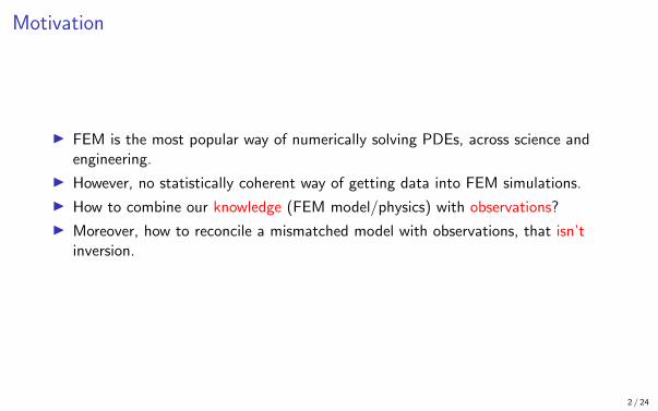
Motivation

I FEM is the most popular way of numerically solving PDEs, across science andengineering.

I However, no statistically coherent way of getting data into FEM simulations.

I How to combine our knowledge (FEM model/physics) with observations?

I Moreover, how to reconcile a mismatched model with observations, that isn’tinversion.

2 / 24

Talk outline

1. FEM: introducing some notation.

2. The linear statFEM construction, getting data into an FEM simulation, Poisson’sequation in 1D.

3. Extending to the nonlinear, time-dependent case, building on nonlinearstate-space modelling/DA.

4. Case study: solitons, the Korteweg-de Vries equation, and applying the filteringmethods.

3 / 24

Section 1

The statistical finite element method (statFEM)

4 / 24

FEM

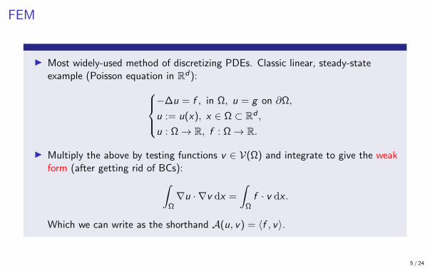
I Most widely-used method of discretizing PDEs. Classic linear, steady-stateexample (Poisson equation in Rd):

−∆u = f , in Ω, u = g on ∂Ω,

u := u(x), x ∈ Ω ⊂ Rd ,

u : Ω→ R, f : Ω→ R.

I Multiply the above by testing functions v ∈ V(Ω) and integrate to give the weakform (after getting rid of BCs):∫

Ω∇u · ∇v dx =

∫Ωf · v dx .

Which we can write as the shorthand A(u, v) = 〈f , v〉.

5 / 24

FEM

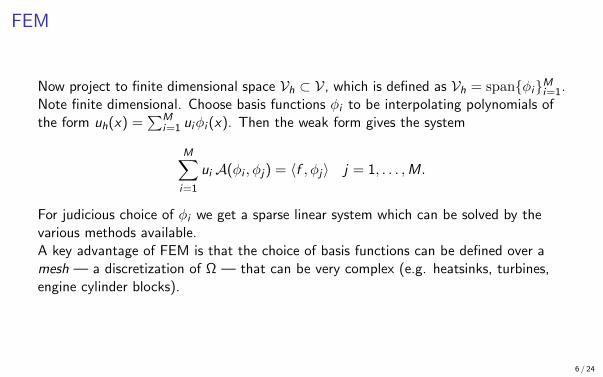
Now project to finite dimensional space Vh ⊂ V, which is defined as Vh = spanφiMi=1.Note finite dimensional. Choose basis functions φi to be interpolating polynomials ofthe form uh(x) =

∑Mi=1 uiφi (x). Then the weak form gives the system

M∑i=1

ui A(φi , φj) = 〈f , φj〉 j = 1, . . . ,M.

For judicious choice of φi we get a sparse linear system which can be solved by thevarious methods available.A key advantage of FEM is that the choice of basis functions can be defined over amesh — a discretization of Ω — that can be very complex (e.g. heatsinks, turbines,engine cylinder blocks).

6 / 24

The statFEM construction

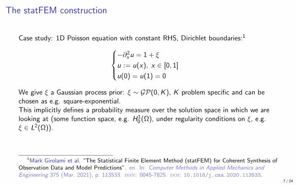
Case study: 1D Poisson equation with constant RHS, Dirichlet boundaries:1−∂2

xu = 1 + ξ

u := u(x), x ∈ [0, 1]

u(0) = u(1) = 0

We give ξ a Gaussian process prior: ξ ∼ GP(0,K ), K problem specific and can bechosen as e.g. square-exponential.This implicitly defines a probability measure over the solution space in which we arelooking at (some function space, e.g. H1

0 (Ω), under regularity conditions on ξ, e.g.ξ ∈ L2(Ω)).

1Mark Girolami et al. “The Statistical Finite Element Method (statFEM) for Coherent Synthesis ofObservation Data and Model Predictions”. en. In: Computer Methods in Applied Mechanics andEngineering 375 (Mar. 2021), p. 113533. issn: 0045-7825. doi: 10.1016/j.cma.2020.113533.

7 / 24

Deriving the prior

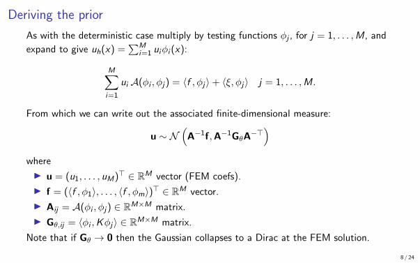
As with the deterministic case multiply by testing functions φj , for j = 1, . . . ,M, and

expand to give uh(x) =∑M

i=1 uiφi (x):

M∑i=1

ui A(φi , φj) = 〈f , φj〉+ 〈ξ, φj〉 j = 1, . . . ,M.

From which we can write out the associated finite-dimensional measure:

u ∼ N(

A−1f,A−1GθA−>)

where

I u = (u1, . . . , uM)> ∈ RM vector (FEM coefs).

I f = (〈f , φ1〉, . . . , 〈f , φm〉)> ∈ RM vector.

I Aij = A(φi , φj) ∈ RM×M matrix.

I Gθ,ij = 〈φi ,Kφj〉 ∈ RM×M matrix.

Note that if Gθ → 0 then the Gaussian collapses to a Dirac at the FEM solution.

8 / 24

Prior measure

0.0 0.2 0.4 0.6 0.8 1.0x

0.00

0.02

0.04

0.06

0.08

0.10

0.12

0.14

0.16

u

Prior

Figure: StatFEM prior: 1D Poisson example asdefined by the previous slide. Mean shown asblue line, 95% probability intervals shown asblue ribbon.

I GP introduces natural uncertaintyinside of the PDE solution.

I This uncertainty can be characterizedby the a priori chosen GP parameters.

I These parameters can be chosen torepresent physically relevantlength/space-scales.

I At one level above (choice ofcovariance function): smoothness.

9 / 24

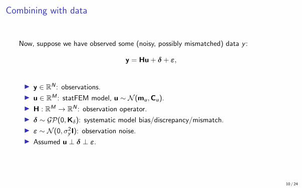
Combining with data

Now, suppose we have observed some (noisy, possibly mismatched) data y :

y = Hu + δ + ε,

I y ∈ RN : observations.

I u ∈ RM : statFEM model, u ∼ N (mu,Cu).

I H : RM → RN : observation operator.

I δ ∼ GP(0,Kδ): systematic model bias/discrepancy/mismatch.

I ε ∼ N (0, σ2y I): observation noise.

I Assumed u ⊥ δ ⊥ ε.

10 / 24

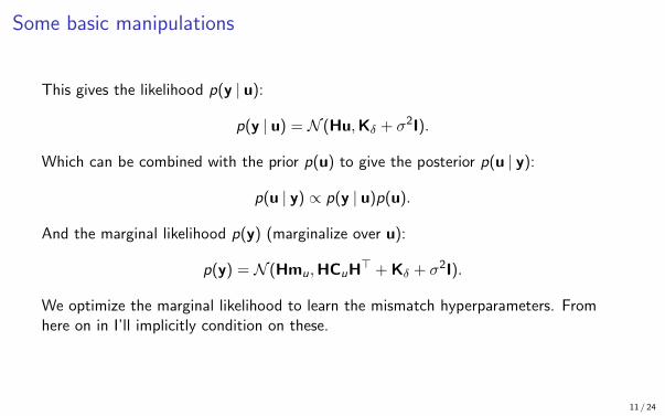
Some basic manipulations

This gives the likelihood p(y | u):

p(y | u) = N (Hu,Kδ + σ2I).

Which can be combined with the prior p(u) to give the posterior p(u | y):

p(u | y) ∝ p(y | u)p(u).

And the marginal likelihood p(y) (marginalize over u):

p(y) = N (Hmu,HCuH> + Kδ + σ2I).

We optimize the marginal likelihood to learn the mismatch hyperparameters. Fromhere on in I’ll implicitly condition on these.

11 / 24

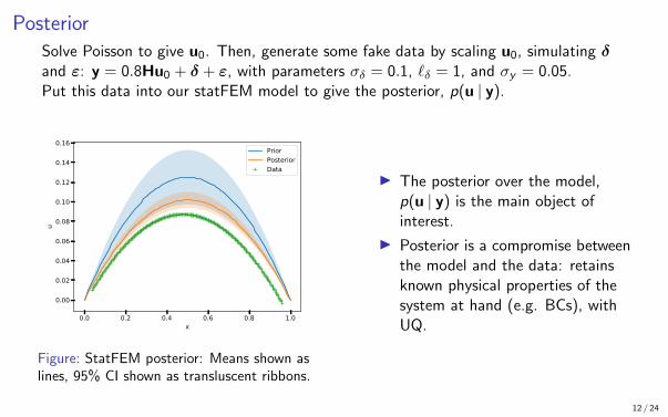
PosteriorSolve Poisson to give u0. Then, generate some fake data by scaling u0, simulating δand ε: y = 0.8Hu0 + δ + ε, with parameters σδ = 0.1, `δ = 1, and σy = 0.05.Put this data into our statFEM model to give the posterior, p(u | y).

0.0 0.2 0.4 0.6 0.8 1.0x

0.00

0.02

0.04

0.06

0.08

0.10

0.12

0.14

0.16

u

PriorPosteriorData

Figure: StatFEM posterior: Means shown aslines, 95% CI shown as transluscent ribbons.

I The posterior over the model,p(u | y) is the main object ofinterest.

I Posterior is a compromise betweenthe model and the data: retainsknown physical properties of thesystem at hand (e.g. BCs), withUQ.

12 / 24

Section 2

Nonlinear problems

13 / 24

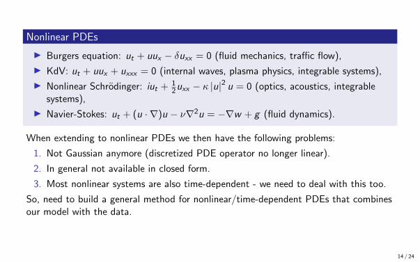
Nonlinear PDEs

I Burgers equation: ut + uux − δuxx = 0 (fluid mechanics, traffic flow),

I KdV: ut + uux + uxxx = 0 (internal waves, plasma physics, integrable systems),

I Nonlinear Schrodinger: iut + 12uxx − κ |u|

2 u = 0 (optics, acoustics, integrablesystems),

I Navier-Stokes: ut + (u · ∇)u − ν∇2u = −∇w + g (fluid dynamics).

When extending to nonlinear PDEs we then have the following problems:

1. Not Gaussian anymore (discretized PDE operator no longer linear).

2. In general not available in closed form.

3. Most nonlinear systems are also time-dependent - we need to deal with this too.

So, need to build a general method for nonlinear/time-dependent PDEs that combinesour model with the data.

14 / 24

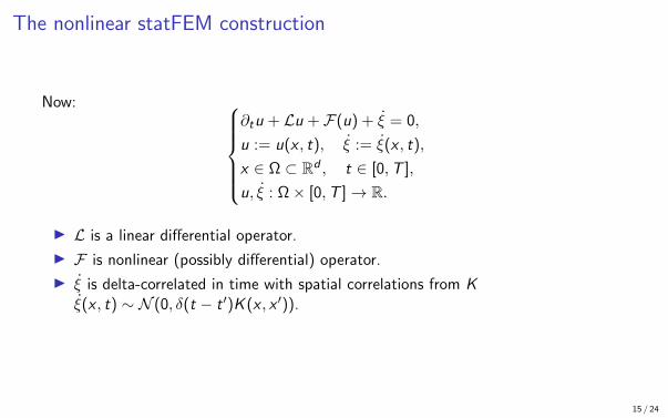
The nonlinear statFEM construction

Now: ∂tu + Lu + F(u) + ξ = 0,

u := u(x , t), ξ := ξ(x , t),

x ∈ Ω ⊂ Rd , t ∈ [0,T ],

u, ξ : Ω× [0,T ]→ R.

I L is a linear differential operator.

I F is nonlinear (possibly differential) operator.

I ξ is delta-correlated in time with spatial correlations from Kξ(x , t) ∼ N (0, δ(t − t ′)K (x , x ′)).

15 / 24

The nonlinear statFEM construction

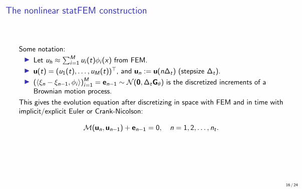
Some notation:

I Let uh ≈∑M

i=1 ui (t)φi (x) from FEM.

I u(t) = (u1(t), . . . , uM(t))>, and un := u(n∆t) (stepsize ∆t).

I (〈ξn − ξn−1, φi 〉)Mi=1 = en−1 ∼ N (0,∆tGθ) is the discretized increments of aBrownian motion process.

This gives the evolution equation after discretizing in space with FEM and in time withimplicit/explicit Euler or Crank-Nicolson:

M(un,un−1) + en−1 = 0, n = 1, 2, . . . , nt .

16 / 24

Conditioning on data

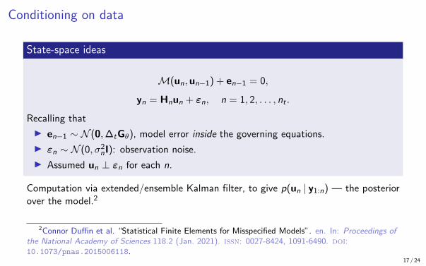
State-space ideas

M(un,un−1) + en−1 = 0,

yn = Hnun + εn, n = 1, 2, . . . , nt .

Recalling that

I en−1 ∼ N (0,∆tGθ), model error inside the governing equations.

I εn ∼ N (0, σ2nI): observation noise.

I Assumed un ⊥ εn for each n.

Computation via extended/ensemble Kalman filter, to give p(un | y1:n) — the posteriorover the model.2

2Connor Duffin et al. “Statistical Finite Elements for Misspecified Models”. en. In: Proceedings ofthe National Academy of Sciences 118.2 (Jan. 2021). issn: 0027-8424, 1091-6490. doi:10.1073/pnas.2015006118.

17 / 24

Section 3

Internal waves: case study

18 / 24

Case study: waves in a tub

WG3WG2WG1

ϑ

L

Hh2

h1

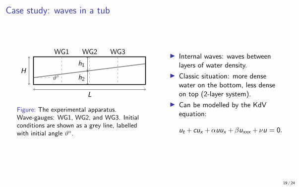
Figure: The experimental apparatus.Wave-gauges: WG1, WG2, and WG3. Initialconditions are shown as a grey line, labelledwith initial angle ϑ.

I Internal waves: waves betweenlayers of water density.

I Classic situation: more densewater on the bottom, less denseon top (2-layer system).

I Can be modelled by the KdVequation:

ut + cux +αuux +βuxxx + νu = 0.

19 / 24

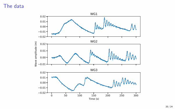
The data

0.020.010.000.010.02

WG1

0.01

0.00

0.01

0.02

Wav

e am

plitu

de (m

) WG2

0 50 100 150 200 250 300Time (s)

0.020.010.000.010.02

WG3

20 / 24

Model specificaton + setup

I Assume dynamics are modelled by the KdV equation:

ut + cux + αuux + βuxxx + νu + ξ = 0.

Solving over x ∈ [0, 6] m, t ∈ [0, 300] s.

I Discretize with FEM in space, Crank-Nicolson in time, to give base equation:

M(un,un−1) + en−1 = 0, n = 1, 2, . . . , nt .

I Data arrives every timestep

yn = Hnun + εn, n = 1, 2, . . . , nt .

I Use EnKF to compute the posterior over the model p(un | y1:n).

21 / 24

Results

0.01

0.00

0.01

A Posterior at wave gauge locationsDataeKdVPosterior

0.02

0.01

0.00

0.01

0.02

t = 75.0

B Posterior profilePosteriorData

0.005

0.000

0.005

0.010

disp

lace

men

t (m

)

0.02

0.01

0.00

0.01

t = 150.0

0 50 100 150 200 250 300t (s)

0.01

0.00

0.01

0 1 2 3 4 5 6x (m)

0.01

0.00

0.01

t = 225.0

22 / 24

Conclusions

StatFEM provides synthesis of data and FEM models: posterior p(u | y).StatFEM methodology has now been developed for linear and nonlinear PDEs.Full details see [2] for the linear case and [1] for the nonlinear extension.Code available at https://github.com/connor-duffin/statkdv-paper.

Future work

Numerical speed-ups where possible, defining the method on the Hilbert space,possibly RKHS connections.Applications to structural monitoring, reaction-diffusion systems (nonlinear oscillators),fluid mechanics.Further investigation of model mismatch — more physically meaningful alternatives toKennedy-O’Hagan?

23 / 24

References

Connor Duffin et al. “Statistical Finite Elements for Misspecified Models”. en. In:Proceedings of the National Academy of Sciences 118.2 (Jan. 2021). issn:0027-8424, 1091-6490. doi: 10.1073/pnas.2015006118.

Mark Girolami et al. “The Statistical Finite Element Method (statFEM) forCoherent Synthesis of Observation Data and Model Predictions”. en. In:Computer Methods in Applied Mechanics and Engineering 375 (Mar. 2021),p. 113533. issn: 0045-7825. doi: 10.1016/j.cma.2020.113533.

24 / 24