Nonlinear Design of Active Suspensions�Jung-Shan Lin and Ioannis Kanellakopoulosy

IEEE Control Systems Magazine, vol. 17, pp. 45–49.

This paper develops a new nonlinear backstepping design for the control of active suspension systems, whichimproves the inherent tradeoff between ride quality and suspension travel. The novelty is in the use of a non-linear filter whose effective bandwidth depends on the magnitude of the suspension travel. This intentionalintroduction of nonlinearity, which is readily accommodated by backstepping, results in a design that is funda-mentally different from previous ones: as the suspension travel changes, the controller smoothly shifts its focusbetween the conflicting objectives of ride comfort and rattlespace utilization, softening the suspension whensuspension travel is small and stiffening it as it approaches the travel limits. Thus, our nonlinear design allowsthe closed-loop system to behave differently in different operating regions, thereby eliminating the dilemmaof whether to use a soft or stiff suspension setting. The improvement achieved with our design is illustratedthrough comparative simulations.

INTRODUCTION

When designing vehicle suspensions, the dual objective is to minimize the vertical forces transmitted tothe passengers (i.e., to minimize vertical car body acceleration) for passenger comfort, and to maximize thetire-to-road contact (i.e., to minimize wheelhop) for handling and safety. While traditional passive suspensionscan negotiate this tradeoff effectively,active suspension systems have the potential to improve both ride qualityand handling performance, with the important secondary benefits of better braking and cornering because ofreduced weight transfer. This improvement, of course, is conditional upon the use of feedback to controlthe hydraulic actuators; several control methods have beenapplied to this problem, most notably skyhookdesigns [2, 3, 14, 15] and optimal control [5–7, 13, 17, 18].

In the process of enhancing passenger comfort and road handling, active suspensions introduce the addi-tional considerations of suspension travel and power consumption, which must be factored into the overall de-sign goals. While the ride/handling tradeoff is prevalent in most approaches [5–7], the ride/rattlespace tradeoffis not explicitly addressed, even though it may be a more fundamental one: to decrease the vertical accelera-tion of the car body, it is necessary to use more suspension travel. This increases the likelihood of hitting thesuspension travel limits when driving over a speed bump or into a pothole, which causes not only considerablepassenger discomfort but also increased wear and tear of vehicle components. Hence, active suspensions shouldhave the ability to behave differently on smooth and rough roads; the desired response should be soft in order toenhance ride comfort, but when the road surface is too rough the suspension should stiffen up to avoid hittingits limits.� A version of this article was originally presented at the 34th IEEE Conference on Decision and Control, New Orleans, LA,December 11–13, 1995. This work was supported in part by NSF through Grants ECS-9309402 and ECS-9502945 and in part byUCLA through the SEAS Dean’s Fund.yThe authors are with the Department of Electrical Engineering, UCLA, Los Angeles, CA 90095-1594. E-mail: jlin@ee.ucla.edu,ioannis@ee.ucla.edu.

In this paper we propose a new nonlinear design aimed at accommodating and improving the tradeoffbetween ride quality and suspension travel. The starting point is the backstepping design methodology [8, 10],whose inherent flexibility can be exploited to satisfy theseconflicting control objectives. The novel featureof our backstepping design is the intentional introductionof nonlinearity into the definition of the regulatedvariable, which is defined as the difference between the car body displacement and the output of a nonlinearfilter. The input to this filter is the wheel displacement, andits effective bandwidth is a nonlinear functionof suspension travel. The resulting response is soft—for enhancing passenger comfort—when the suspensiontravel is small, but stiffens up very quickly as the suspension approaches its travel limits, to avoid hitting them.Hence, the intentional introduction of nonlinearity endows the closed-loop system with the ability to emphasizedifferent objectives in different operating regions relative to responseamplitude.

This amplitude dependence is a property which linear control can never attain, regardless of the designmethod used: the response of a linear controller is always proportional to the amplitude of the error. Thus, ifone chooses the gains so that the suspension travel limits are not reached when going over a large bump, thedesign will be too conservative and the ride quality over smooth roads will suffer.

The remainder of the paper is organized as follows. First of all, we introduce the basic passive quarter-carsuspension system and discuss the design ofparallel active suspensions in which the hydraulic actuator forceis viewed as the control input. This simplification allows usto illustrate the limitations and basic propertiesof active suspensions via frequency-domain analysis. Then, we consider the full-blown quarter-car active sus-pension model, including the dynamics of the hydraulic actuator, and use it to design a nonlinear backsteppingcontroller which meets the desired control objectives. This controller is evaluated using the simulation resultswhich compare the performance of our nonlinear active design to that of a passive suspension system. Finally,some concluding remarks are given for further research.

SIMPLIFIED MODELS

Passive Suspension

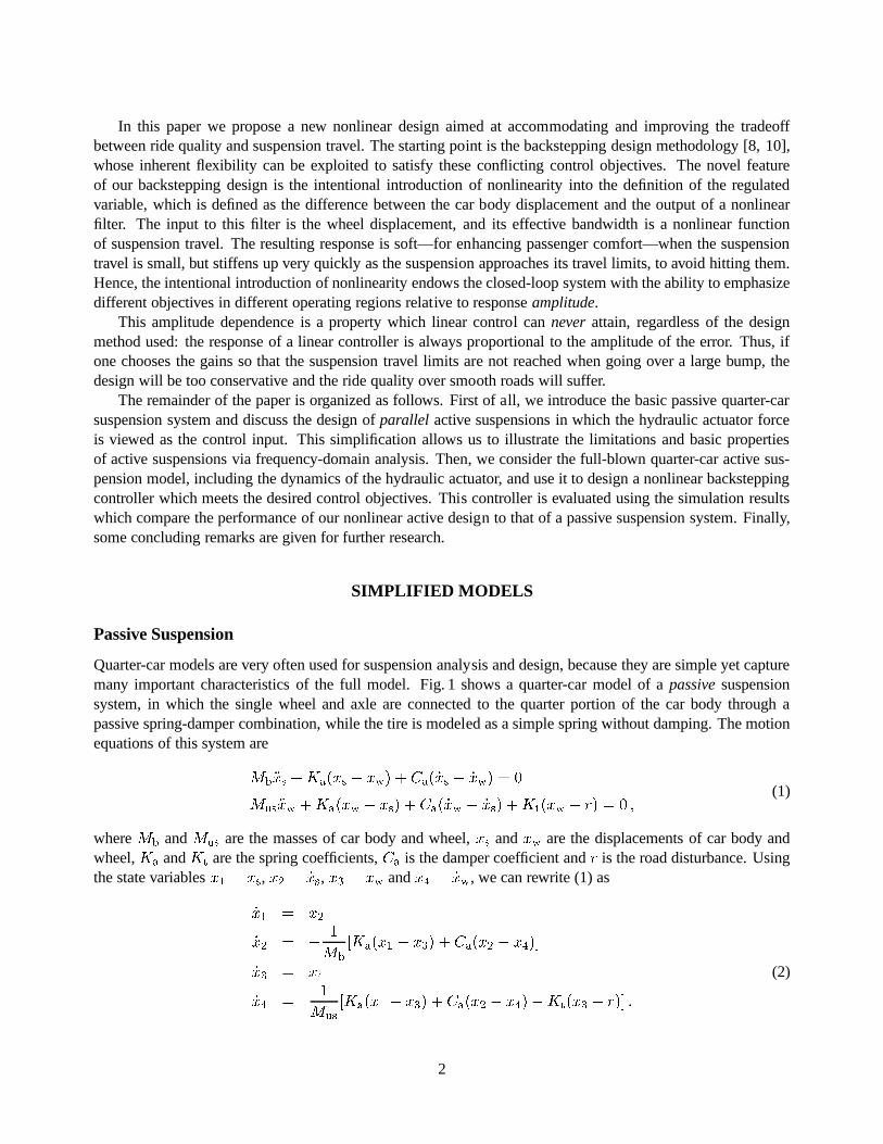
Quarter-car models are very often used for suspension analysis and design, because they are simple yet capturemany important characteristics of the full model. Fig. 1 shows a quarter-car model of apassive suspensionsystem, in which the single wheel and axle are connected to the quarter portion of the car body through apassive spring-damper combination, while the tire is modeled as a simple spring without damping. The motionequations of this system areMb�xs +Ka(xs � xw) + Ca( _xs � _xw) = 0Mus�xw +Ka(xw � xs) + Ca( _xw � _xs) +Kt(xw � r) = 0 ; (1)

whereMb andMus are the masses of car body and wheel,xs andxw are the displacements of car body andwheel,Ka andKt are the spring coefficients,Ca is the damper coefficient andr is the road disturbance. Usingthe state variablesx1 = xs, x2 = _xs, x3 = xw andx4 = _xw, we can rewrite (1) as_x1 = x2_x2 = � 1Mb [Ka(x1 � x3) + Ca(x2 � x4)]_x3 = x4 (2)_x4 = 1Mus [Ka(x1 � x3) + Ca(x2 � x4)�Kt(x3 � r)] :

2

�������� KaCae6xs6xw6r���������������������������� ��������

Mbcar bodywheel Mus Kt�������

���

Figure 1: Quarter-car model with passive spring/damper only.

Since (2) is a linear system, we can use frequency domain analysis. If we consider the displacements ofcar body and wheel as the outputs and the road disturbancer as the input, and denote the constantsa1 = CaMb ,a2 = KaMb , a3 = CaMus , a4 = KaMus and!20 = KtMus (!0 is the natural frequency of the unsprung subsystem), thenfrom (2) we have the following transfer functions:H1p(s) = X1(s)R(s) = !20(a1s+ a2)�p(s)H3p(s) = X3(s)R(s) = !20(s2 + a1s+ a2)�p(s) ; (3)

whereX1(s), X3(s) andR(s) are the Laplace transform functions ofx1(t), x3(t) andr(t), and�p(s) = s4 + (a1 + a3)s3 + (a2 + a4 + !20)s2 + a1!20s+ a2!20 : (4)

These transfer functions will be used for comparison purposes later on.

Active Suspension

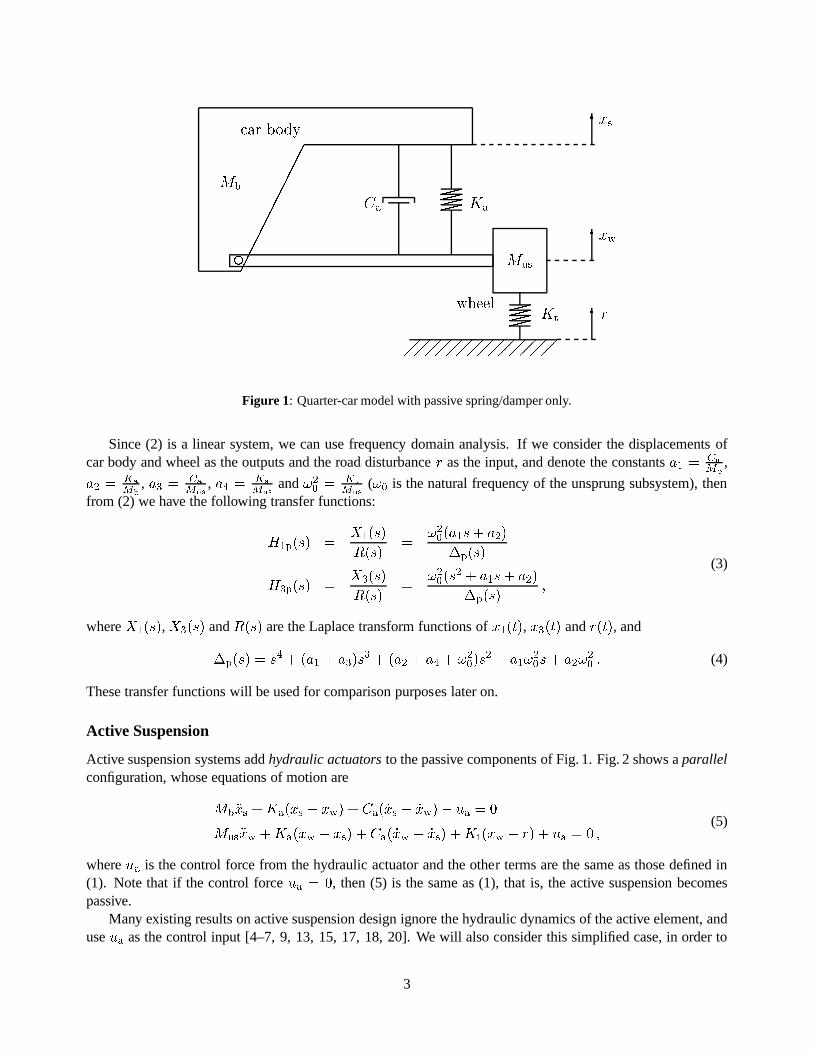
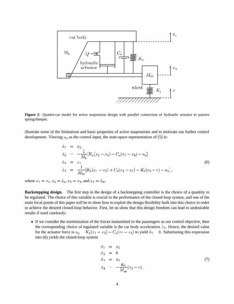
Active suspension systems addhydraulic actuators to the passive components of Fig. 1. Fig. 2 shows aparallelconfiguration, whose equations of motion areMb�xs +Ka(xs � xw) + Ca( _xs � _xw)� ua = 0Mus�xw +Ka(xw � xs) +Ca( _xw � _xs) +Kt(xw � r) + ua = 0 ; (5)

whereua is the control force from the hydraulic actuator and the other terms are the same as those defined in(1). Note that if the control forceua = 0, then (5) is the same as (1), that is, the active suspension becomespassive.

Many existing results on active suspension design ignore the hydraulic dynamics of the active element, anduseua as the control input [4–7, 9, 13, 15, 17, 18, 20]. We will also consider this simplified case, in order to

3

Q -hydraulicactuator �������� KaCae6xs6xw6r���������������������������� ��������

Mbcar bodywheel Mus Kt�������

���

Figure 2: Quarter-car model for active suspension design with parallel connection ofhydraulic actuator to passivespring/damper.

illustrate some of the limitations and basic properties of active suspensions and to motivate our further controldevelopment. Viewingua as the control input, the state-space representation of (5)is:_x1 = x2_x2 = � 1Mb [Ka(x1 � x3) +Ca(x2 � x4)� ua]_x3 = x4 (6)_x4 = 1Mus [Ka(x1 � x3) + Ca(x2 � x4)�Kt(x3 � r)� ua] ;wherex1 = xs, x2 = _xs, x3 = xw andx4 = _xw.

Backstepping design. The first step in the design of a backstepping controller is the choice of a quantity tobe regulated. The choice of this variable is crucial to the performance of the closed-loop system, and one of themain focal points of this paper will be to show how to exploit the design flexibility built into this choice in orderto achieve the desired closed-loop behavior. First, let us show that this design freedom can lead to undesirableresults if used carelessly:� If we consider the minimization of the forces transmitted tothe passengers as our control objective, then

the corresponding choice of regulated variable is the car body acceleration_x2. Hence, the desired valuefor the actuator force isua = Ka(x1 � x3) + Ca(x2 � x4) to yield _x2 = 0. Substituting this expressioninto (6) yields the closed-loop system_x1 = x2_x2 = 0_x3 = x4 (7)_x4 = � KtMus (x3 � r) :

4

This represents thezero dynamics of the closed-loop system, which consist of anunstable subsystem(double integrator for body position and velocity) and anoscillatory subsystem (wheel position andvelocity). Clearly, this system is not stable, and road disturbance inputs will result in sustained wheeloscillations and even diverging car body displacement.� If we instead choose the body positionx1 as the regulated variable, then the(x1; x2)-subsystem is stabi-lized, while the(x3; x4)-subsystem represents the zero dynamics. A choice ofua which yields_x1 = x2_x2 = �c1x1 � c2x2 ; (8)

will also result in _x3 = x4_x4 = MbMus (c1x1 + c2x2)� KtMus (x3 � r) : (9)

Substitutingx1 = x2 = 0 into (9), we obtain the oscillatory zero dynamics_x3 = x4_x4 = � KtMus (x3 � r) : (10)

The unstable subsystem of (7) has been eliminated with this second choice of regulated variable, but theresulting closed-loop behavior is still not acceptable, since it contains an undamped oscillatory subsys-tem.� If we shift our attention to the minimization of the suspension travel, then the regulated variable becomesx1 � x3: the suspension travel is the difference between the body positionx1 and the wheel positionx3.However, the zero dynamics are again oscillatory as in (10),and hence this design is still not acceptable.

We must therefore choose the regulated variable so as to avoid the oscillatory zero dynamics. One suchchoice is the variable z1 = x1 � �x3 ; (11)

wherex1 is the car body displacement and�x3 is a filtered version of the wheel displacementx3:�x3 = �s+ �x3 : (12)

This choice represents the first step towards the design of a controller which will accommodate the inherenttradeoff between ride quality and rattlespace usage. Let ussee how the choice of the positive constant� affectsthe properties of our active suspension:� For small values of�, (12) is just alow-pass filter. Hence, the regulated variablez1 is essentially equal to

the car body displacementx1 as long as the road input contains only high-frequency components whichare rejected; however, at very low frequencies (constant orslowly changing road elevations) and in steadystate,z1 becomes almost identical to the suspension travelx1 � x3. Thus, as we will see later on, thesustained oscillations are eliminated, and the active suspension rejects only high-frequency road distur-bances, namely the ones which generate large vertical accelerations and cause passenger discomfort.

5

� As the value of� becomeslarger, more high-frequency components of the road input are allowed to passthrough the filter (12). Hence, the regulated variablez1 approximates the suspension travelx1 � x3: thehigh filter bandwidth renders�x3 � x3. As a result, the active suspension becomes stiffer and reduces itsrattlespace use, at the price of significantly reduced passenger comfort.

With this choice of regulated variablez1 defined in (11), the backstepping design procedure consistsof twosteps:

Step 1: We compute the derivative ofz1 as_z1 = _x1 � _�x3= x2 + �(�x3 � x3)= x2 + �(x1 � z1 � x3)= x2 + �(x1 � x3)� �z1 ; (13)

and usex2 as the firstvirtual control variable, for which we choose thestabilizing function�1 = �c1z1 � �(x1 � x3) ; (14)

with c1 a positive design constant. The corresponding error variable is z2 = x2 � �1, and the resulting errorequation is _z1 = �(c1 + �)z1 + z2 : (15)

Step 2: The derivative ofz2 is computed as_z2 = _x2 � _�1= � 1Mb [Ka(x1 � x3) + Ca(x2 � x4)� ua]� [�c1(�c1z1 � �z1 + z2)� �(x2 � x4)] : (16)

Since the actual controlua appears in (16), we choose our control law asua = Mb[�(c2 + c1)z2 + (c21 � 1 + c1�)z1 � �(x2 � x4)]+Ka(x1 � x3) + Ca(x2 � x4) ; (17)

wherec2 is a positive design constant, to render the derivative of the Lyapunov functionVa = 12z21 + 12z22 (18)

negative definite: _Va = �(c1 + �)z21 � c2z22 : (19)

This implies that the error system _z1 = �(c1 + �)z1 + z2_z2 = �c2z2 � z1 (20)

has a globally exponentially stable equilibrium at(z1; z2) = (0; 0).6

Zero dynamics. We started out with the fifth-order system consisting of the active suspension (6) and thelinear filter (12), and ended up with the second-order error system (20). The remaining three states are thus thezero dynamics subsystem of the closed-loop system. To find the zero dynamics, we set the output identicallyequal to zero, i.e.,y = z1 = x1 � �x3 � 0. Hence, we have_y = x2 + �(�x3 � x3) = 0�y = � 1Mb [Ka(x1 � x3) + Ca(x2 � x4)� ua] + �[��(�x3 � x3)� x4] = 0 : (21)

Using the last equation of (21) we substituteKa(x1 � x3) + Ca(x2 � x4)� ua = Mb�[��(�x3 � x3)� x4] (22)

into the _x4-equation of (6) to obtain the zero dynamics:_�x3 = ��(�x3 � x3)_x3 = x4 (23)_x4 = MbMus �[��(�x3 � x3)� x4]� KtMus (x3 � r) ;which is then rewritten in the following matrix form:264 _�x3_x3_x4 375 = 264 �� � 00 0 1��2 MbMus �2 MbMus� KtMus �� MbMus 375264 �x3x3x4 375+ 264 00KtMus 375 r : (24)

Using the Ruth-Hurwitz criterion, it is easy to show that the3�3 matrix in (24) is Hurwitz if and only if� > 0.Therefore, the zero dynamics are exponentially stable for all � > 0.

Frequency domain analysis. If we rewrite the control law (17) asua = �Mb(c2 + c1)fx2 � [�c1(x1 � �x3)� �(x1 � x3)]g+Mb(c21 � 1 + c1�)(x1 � �x3)� �Mb(x2 � x4) +Ka(x1 � x3) + Ca(x2 � x4)= �Mb(c2 + c1)x2 + [Ka � �Mb(c2 + c1)](x1 � x3)+ (Ca � �Mb)(x2 � x4) +Mb[c1(�� c2)� 1](x1 � �x3) ; (25)

then the resulting closed-loop system becomes2666664 _x1_x2_�x3_x3_x43777775 = 2666664 0 1 0 0 0�q1 �(q2 + �) �q3 �q2 �0 0 �� � 00 0 0 0 1mrq1 mr(q2 + �) mrq3 �(mr�q2 + !20) �mr�

37777752666664 x1x2�x3x3x43777775+ 2666664 0000!20

3777775 r ; (26)

wheremr = MbMus , q1 = c2(c1 + �) + 1, q2 = c2 + c1 andq3 = c1(� � c2) � 1. Now we want to computethe transfer functions relating the road inputr to the car body displacementx1 and the wheel travelx3. It is atedious but straightforward task to obtain these transfer functions directly from the state-space representation(26). An equivalent and much simpler way is to utilize the results of our control design, which guaranteesthat the error variablez1 converges to zero exponentially, which means thatx1 approaches�x3 exponentially

7

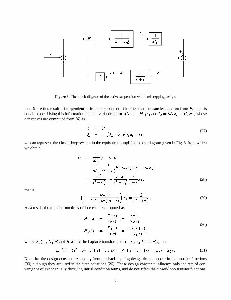
r -M6- Kt - 1s2 + !20 �1 - 1Mus ?M+�� x3�s+ �� x1 = �x3mr -

Figure 3: The block diagram of the active suspension with backstepping design.

fast. Since this result is independent of frequency content, it implies that the transfer function from�x3 to x1 isequal to one. Using this information and the variables�1 = Mbx1 +Musx3 and�2 = Mbx2 +Musx4, whosederivatives are computed from (6) as_�1 = �2_�2 = �!20�1 +Kt(mrx1 + r) ; (27)

we can represent the closed-loop system in the equivalent simplified block diagram given in Fig. 3, from whichwe obtain x3 = 1Mus �1 �mrx1= 1Mus 1s2 + !20Kt(mr�x3 + r)�mr�x3= !20s2 + !20 r � mrs2s2 + !20 �s+ �x3 ; (28)

that is, 1 + mr�s2(s2 + !20)(s+ �)!x3 = !20s2 + !20 r : (29)

As a result, the transfer functions of interest are computedasH1a(s) = X1(s)R(s) = !20��a(s)H3a(s) = X3(s)R(s) = !20(s+ �)�a(s) ; (30)

whereX1(s), X3(s) andR(s) are the Laplace transforms ofx1(t), x3(t) andr(t), and�a(s) = (s2 + !20)(s+ �) +mr�s2 = s3 + �(mr + 1)s2 + !20s+ !20� : (31)

Note that the design constantsc1 andc2 from our backstepping design do not appear in the transfer functions(30) although they are used in the state equations (26). These design constants influence only the rate of con-vergence of exponentially decaying initial condition terms, and do not affect the closed-loop transfer functions.

8

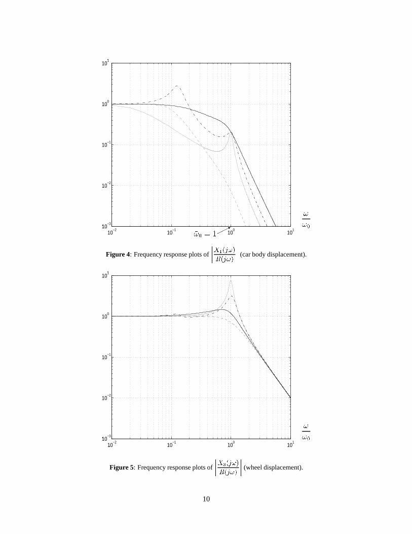
Let us now compare the transfer functions of the passive suspension and of our active suspension with thoseof the “ideal” suspension:H1i(s) = X1(s)R(s) = 1�s2 + 2�opt�s+ 1H3i(s) = X3(s)R(s) = 1(n2�s2 + 2�optn�s+ 1)(�s2 + 2�opt�s+ 1) ; (32)

wheren = 10, �opt = p22 and�s = s!0 . The reasons for viewing (32) as the ideal response are lucidly explainedin [9], where it is also shown that this response cannever be achieved by any suspension, be it passive or active,which exerts forces only between the wheel and the car body, i.e., by any suspension which can be implementedon a road vehicle.

Using the normalized Laplace variable�s, we can rewrite (3) asH1p(s) = �a1�s+ �a2��p(�s) ; H3p(s) = �s2 + �a1�s+ �a2��p(�s) ; (33)

where�a1 = a1!0 , �a2 = a2!20 , �a3 = a3!0 , �a4 = a4!20 and��p(�s) = �s4 + (�a1 + �a3)�s3 + (�a2 + �a4 + 1)�s2 + �a1�s+ �a2 ; (34)

and (30) as H1a(s) = ���a(�s) ; H3a(s) = �s+ ���a(�s) ; (35)

where� = �!0 and ��a(�s) = �s3 + �(mr + 1)�s2 + �s+ � : (36)

These transfer functions are plotted in Figs. 4–7 with the following standard values taken from [2, 3]:Mb = 290 kg Mus = 59 kgKa = 16812 N=m Ca = 1000 N=(m=sec)Kt = 190000 N=m : (37)

Each of these four figures contains frequency response plotsfor four different configurations: the ideal suspen-sion (– – dashed line), the passive suspension (–� dashdot line), and our active suspension with� = 1:5 (thin solid line) and� = 10 ( thick solid line). Figs. 4 and 5 show the frequency response plots of

���X1(j!)R(j!) ���(car body displacement) and

���X3(j!)R(j!) ��� (wheel displacement). The frequency response plots of����!2X1(j!)R(j!) ��� (car

body acceleration) and���X1(j!)�X3(j!)R(j!) ��� (suspension travel) are shown in Figs. 6 and 7 respectively.

As shown in [4, 16, 20], the frequency response plots of any real suspension must pass through certaininvariant points:� In both Fig. 4 and Fig. 6, there is an invariant point at the natural frequency of the unsprung mass!0 =q KtMus (i.e., at�!0 = 1, where the normalized frequency is defined as�! = !!0 ). In particular, at that point

we have jH1p(j!0)j = jH1a(j!0)j = 1mr (� 0:20) (38)j � !20H1p(j!0)j = j � !20H1a(j!0)j = !20mr (� 655) : (39)

9

10−2

10−1

100

101

10−3

10−2

10−1

100

101

��*�!0 = 1 !!0Figure 4: Frequency response plots of

����X1(j!)R(j!) ���� (car body displacement).

10−2

10−1

100

101

10−3

10−2

10−1

100

101

!!0Figure 5: Frequency response plots of

����X3(j!)R(j!) ���� (wheel displacement).

10

10−2

10−1

100

101

10−1

100

101

102

103

��*�!0 = 1 !!0Figure 6: Frequency response plots of

�����!2X1(j!)R(j!) ���� (car body acceleration).

10−2

10−1

100

101

10−3

10−2

10−1

100

101

6�!2 � 0:41 !!0Figure 7: Frequency response plots of

����X1(j!)�X3(j!)R(j!) ���� (suspension travel).

11

� In Fig. 7, there is another invariant point at the natural frequency of the whole quarter-car system!2 =q KtMb+Mus (i.e., �!2 = q 11+mr � 0:41). The corresponding value of the transfer function magnitude isjH1p(j!2)�H3p(j!2)j = jH1a(j!2)�H3a(j!2)j = 1 + 1mr (� 1:20) : (40)

As explained in [9], these invariant properties are a resultof the fact that the suspension forces are appliedonly between a wheel and the car body, and they place insurmountable limitations to what can be achievedby active suspension designs. In particular, as demonstrated by Figs. 4–7, our active suspension design cannotcompletely coincide with the ideal suspension in (32). Nevertheless, it is also clear that with the appropriatechoice of the filter bandwidth� our active suspension design is superior not only to the passive suspension butalso to the ideal one in some frequency ranges. With small� (� = 1:5), the active suspension design reducesboth car body displacement and acceleration compared to thepassive one (cf. Figs. 4 and 6), but increases thesuspension travel as seen in Fig. 7. On the other hand, if� is increased to 10, then the suspension travel can besignificantly reduced, as seen in Fig. 7, but then the car bodydisplacement and acceleration are increased (cf.Figs. 4 and 6).

FULL-ORDER NONLINEAR DESIGN

It is clear from the above analysis that any fixed value of� leads to a compromise between ride quality andrattlespace usage. It is also clear from Figs. 4, 6 and 7 that we should use small values of� to improve ridequality and large values to reduce suspension travel. But how can the two be combined? One possibility isto use the magnitude of suspension travel as the criterion for emphasizing one control objective more than theother:� As long as the suspension travel is small, the controller should be allowed to focus on passenger comfort,

which means that the bandwidth of the filter should be low.� When the suspension travel becomes large, the control objective should shift to preventing the suspensionfrom hitting its travel limits, by using a high bandwidth filter.

Nonlinear Filter

To realize this nonlinear control objective, we replace thelinear filter (12) by anonlinear one, whose effectivebandwidth changes with the magnitude of the suspension travel:_�x3 = �(�0 + �1'(�))(�x3 � x3) : (41)

In (41), �0 is a positive constant,�1 is a nonnegative constant,� = x1 � x3 is the suspension travel, and thenonlinear function'(�), shown in Fig. 8, is defined as'(�) = 8>>>>>>><>>>>>>>:

�� �m1m2 �4 ; � > m10 ; j�j � m1�� +m1m2 �4 ; � < �m1 ; (42)

12

-6

�'(�)01 -� m1-� m1 -�m2-�m2

Figure 8: The nonlinear function'(�) defined in (42).

wherem1 � 0 andm2 > 0. Note that if�1 = 0, this nonlinear filter (41) is identical to the linear filter in (12)with � = �0.

This nonlinearity contains a deadzone defined by�m1 � � � m1; hence it remains “dormant” as longas the suspension travel is smaller thanm1 in magnitude. In that region, the bandwidth of the nonlinearfil-ter (41) is constant and equal to�0, which can be chosen small to satisfy the passenger comfort requirement; thenonlinear filter then becomes identical to the linear filter shown to possess good ride quality properties in theprevious section. As soon as the suspension travel leaves this deadzone, the nonlinearity'(�) is activated, andit rapidly increases the effective bandwidth of the filter, thereby shifting the control objective to minimizationof suspension travel. Thus, the intentional introduction of nonlinearity into the control objective allows thecontroller to react differently in different operating regimes.

Hydraulic Dynamics

In the previous section we neglected the dynamics of the hydraulic actuator, because we wanted to illustrate thebasic ideas which led to the development of the nonlinear filter (41)–(42). Now that we are ready to embark onthe actual nonlinear control design, we include the hydraulic dynamics and design a controller for the full-orderquarter-car model. The model we use for the hydraulic actuator and its spool valve is the same as in [2, 3]; thefollowing discussion of the basic concepts is adapted from [1, 12, 16, 19].

The hydraulic actuator we use here is a four-way valve-piston system. We know the forceua from theactuator is ua = APL ; (43)

whereA is the piston area andPL is the pressure drop across the piston. Following Merritt [12], the derivativeof PL is given by: Vt4�e _PL = Q� CtpPL �A( _xs � _xw) ; (44)

whereVt is the total actuator volume,�e is the effective bulk modulus,Q is the hydraulic load flow, andCtp isthe total leakage coefficient of the piston. In addition, theservovalve load flow equation is given byQ = Cdwxvs1� [Ps � sgn(xv)PL] ; (45)

13

whereCd is the discharge coefficient,w is the spool valve area gradient,xv is the valve displacement from its“closed” position,� is the hydraulic fluid density, andPs is the supply pressure. However, since here we wantto include the possibility of the termPs � sgn(xv)PL becoming negative, we replace (45) with the correctedflow equation: Q = sgn[Ps � sgn(xv)PL]Cdwxvs1� jPs � sgn(xv)PLj : (46)

Finally, the spool valve displacement is controlled by the input to the servovalveu, which could be a currentor a voltage. The valve dynamics are approximated by a linearfilter with time constant� . This is a goodapproximation if the frequency is not too high, and it is regularly used by active suspension designers in industry.A more elaborate model would include stiction and deadzone nonlinearities commonly found in inexpensivevalves. Without loss of generality, the steady-state gain is taken to be one:_xv = 1� (�xv + u) : (47)

Choosing the state variablesx1 = xs, x2 = _xs, x3 = xw, x4 = _xw, x5 = PL andx6 = xv, we rewrite (5),(43)–(44) and (46)–(47) as follows:_x1 = x2_x2 = � 1Mb [Ka(x1 � x3) + Ca(x2 � x4)�Ax5]_x3 = x4_x4 = 1Mus [Ka(x1 � x3) + Ca(x2 � x4)�Kt(x3 � r)�Ax5] (48)_x5 = ��x5 � �A(x2 � x4) + x6w3_x6 = 1� (�x6 + u) ;where� = 4�eVt , � = �Ctp, = �Cdwq 1� andw3 = sgn[Ps � sgn(x6)x5]qjPs � sgn(x6)x5j : (49)

Backstepping Design

The choice of regulated variable we use here is the same as (11), that is,z1 = x1 � �x3 ; (50)

wherex1 is the car body displacement, but here�x3 is the output of the nonlinear filter (41). The presence ofthe nonlinearity'(�) can easily be handled by the backstepping design procedure,which was developed fornonlinear systems; the design remains qualitatively the same as it would be with the linear filter (12), and theonly effect is the appearance of some new terms in the expressions. Our backstepping design procedure whichcontains four steps is outlined next, and its details are presented in the Appendix.

Step 1: Starting with the regulated variablez1 from (50), we usex2 as the virtual control in the_z1-equation,and introduce the error variablez2 = x2 � �1, where�1 is the firststabilizing function.

Step 2: Let �x5 = �x5, with � a positive constant which rescalesx5 (this rescaling is very useful for reducingthe numerical integration errors in our simulations). We use �x5 as the virtual control in the_z2-equation, definez3 = �x5 � �2, and choose the second stabilizing function�2.

14

Step 3: Our choice of virtual control in the_z3-equation isx6w3, with w3 defined in (49). We then introducethe error variablez4 = x6w3 � �3 and choose the third stabilizing function�3.Step 4: Since the actual controlu appears in the_z4-equation, we can finally determine the control lawu in thisstep. The resulting control law is chosen as u = �w3�4 ; (51)

where�4 is the last stabilizing function. With this choice, we have the closed-loop error system (in thez-coordinates) as follows:_z1 = �c1z1 � (�0 + �1'(�))z1 + z2_z2 = �c2z2 � z1 + A�Mb z3_z3 = �c3z3 � A�Mb z2 + � z4 + d3r + n3h3r � b3h23z3 (52)_z4 = �c4z4 � � z3 + d4r + n4h4r � b4h24z4 ;wherec1, c2, c3, c4, b3 andb4 are positive design constants andn3, d3, h3, n4, d4 andh4 are defined in theAppendix.

Now let us consider the partial Lyapunov functionV = 12(z21 + z22 + z23 + z24) : (53)

From (52), the derivative of (53) is computed as_V = z1 _z1 + z2 _z2 + z3 _z3 + z4 _z4= �(c1 + �0 + �1'(�))z21 � c2z22 � c3z23 � c4z24+ d3z3r + n3h3z3r � b3h23z23 + d4z4r + n4h4z4r � b4h24z24 : (54)

Since the road disturbancer is unknown, we can not cancel the cross terms in (54) by using the controlu.However, the boundedness of all the error signals is guaranteed for any positive values of the design constantsc1, c2, c3, c4, b3 andb4. Indeed, by completing squares, we rewrite (54) as_V = �(c1 + �0 + �1'(�))z21 � c2z22 � 12c3z23 � 12c4z24� c32 �z3 � d3c3 r�2 + d232c3 r2 � c42 �z4 � d4c4 r�2 + d242c4 r2� b3 �h3z3 � n32b3 r�2 + n234b3 r2 � b4 �h4z4 � n42b4 r�2 + n244b4 r2� �(c1 + �0 + �1'(�))z21 � c2z22 � 12c3z23 � 12c4z24+ d232c3 + d242c4 + n234b3 + n244b4! r2 : (55)

It should be clear from (55) that any bounded road disturbance r will generate bounded error signals, since_Vwill become negative for large enough values of the error statesz1, z2, z3 andz4. This is true with any positivechoices forc1, c2, c3, c4, b3 andb4, although very small values of these constants may lead to unacceptablylarge errors.

15

Zero Dynamics

The backstepping design procedure involved four steps, andresulted in a fourth-order error system with statesz1, z2, z3 andz4. However, the original suspension system contains a total of seven states (including the state�x3, the output of the nonlinear filter in (41)), so the zero dynamics of the resulting closed-loop system stillconsist of three states. To find the zero dynamics, we set the outputy = z1 = x1 � �x3 � 0. Hence, we obtain_y = x2 + (�0 + �1'(�))(�x3 � x3) = 0�y = � 1Mbw0 + �1 d'd� (x2 � x4)(�x3 � x3) (56)+ (�0 + �1'(�))[�(�0 + �1'(�))(�x3 � x3)� x4] = 0 :Substitution of (56) into (41) and (48) yields the zero dynamics:_�x3 = �(�0 + �1'(��))��_x3 = x4 (57)_x4 = MbMus [�(�0 + �1'(��))�� � x4](�0 + �1'(��) + �1 d'd�� ��)� KtMus (x3 � r) ;where�� = �x3 � x3. If �1 = 0, then (57) becomes264 _�x3_x3_x4 375 = 264 ��0 �0 00 0 1��20 MbMus �20 MbMus� KtMus ��0 MbMus 375264 �x3x3x4 375+ 264 00KtMus 375 r : (58)

This is the same as the zero dynamics in (24) with� = �0, so we conclude that the zero dynamics (58) are stablefor all �0 > 0. If �1 > 0, then we consider the following system (obtained from (57) with r = 0):_�� = ����� � x4_x3 = x4 (59)_x4 = MbMus (����� � x4) �'� KtMusx3 ;where�� = �0+�1'(��) (> 0) and �' = ��+�1 d'd�� �� (> 0). To show that (59) is asymptotically stable, we considerthe Lyapunov function V0 = 12��2��2 + 12 KtMbx23 + 12MusMb x24 ; (60)

whose derivative is computed as_V0 = ���1 d'd�� (����� � x4)��2 + ��2��(����� � x4) + KtMbx3x4 + x4[(����� � x4) �'� KtMbx3]= ���2�1 d'd�� ��3 � ���1d'd�� x4��2 � ��3��2 � ��2��x4 � �� �'x4�� � �'x24= ���2(��+ �1d'd�� ��)��2 � ( �'+ ��+ �1 d'd�� ��)����x4 � �'x24= ���2 �'��2 � 2 �'����x4 � �'x24= � �'(���� + x4)2� 0 : (61)

16

Using LaSalle’s invariance theorem, we conclude that the equilibrium point (��; x3; x4) = (0; 0; 0) of the system(59) is asymptotically stable, since it is the largest invariant set of (59) contained in the set where the Lyapunovderivative is zero, i.e., in the setE = n(��; x3; x4) 2 IR3 j _V0 = 0o.

SIMULATION RESULTS

To verify that our new nonlinear control design achieves thedesired objective, we simulated the resultingclosed-loop system and compare it to both a passive suspension system and to an active design with the linearfilter; we used the parameter values from (37) and the following standard values from [2, 3]:� = 4:515 � 1013 N=m5 � = 1 sec�1 = 1:545 � 109 N=(m5=2 kg1=2) � = 1=30 secPs = 10342500 Pa (1500 psi) A = 3:35 � 10�4 m2 : (62)

Since the value of the supply pressurePs is so large, we used� = 10�7 to rescale the statex5 for improvednumerical accuracy. We also assumed the following limits:� Suspension travel limits:� 8 cm.� Spool valve displacement limits:� 1 cm.

Furthermore, sincew3 in (49) appears in the denominator of (51), we employed the following modification toavoid division by zero:� Setw3 = 1 if 0 � w3 � 1 and setw3 = �1 if �1 � w3 < 0 in the denominator (only) of the control

law (51).

We chose the road disturbancer as a single bump represented in the following form:r = ( a(1� cos 8�t) ; 0:5 � t � 0:750 ; otherwise ; (63)

and ran three simulations witha set to0:025, 0:038 and0:055 m, that is, with the height of the bump equal to5, 7:6 and11 cm. In addition, we chose the design constants as follows:c1 = c2 = c3 = c4 = 200 ; b3 = b4 = 0:01�0 = 1:5 ; m1 = 0:055 ; m2 = 0:005 : (64)

The choice ofm1 is particularly important, since it defines the width of the deadzone in which the nonlinearityof the filter remains inactive. Since our suspension travel limits here are� 8 cm, we chose the deadzone to be� 5:5 cm.

Our simulations compare a standard passive suspension (dotted line) with two active suspension designs:one that does not attempt to prevent the suspension from hitting its travel limits, i.e, uses�1 = 0 (dashed line),and one that uses�1 = 0:0125 (solid line). We show plots of body acceleration, body travel, wheel travel andsuspension travel for three different magnitudes of the road disturbance:

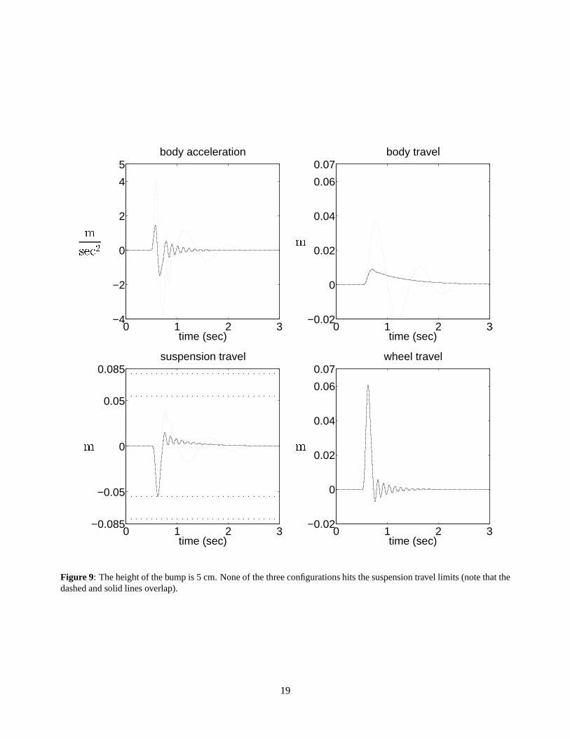
1. Fig. 9 usesa = 0:025 m (road bump height 5 cm),

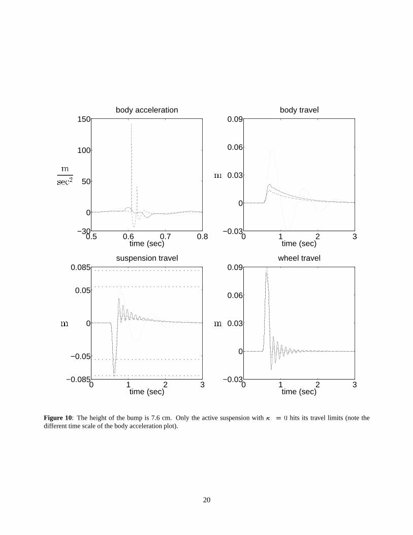
2. Fig. 10 is witha = 0:038 m (road bump height 7.6 cm), and

17

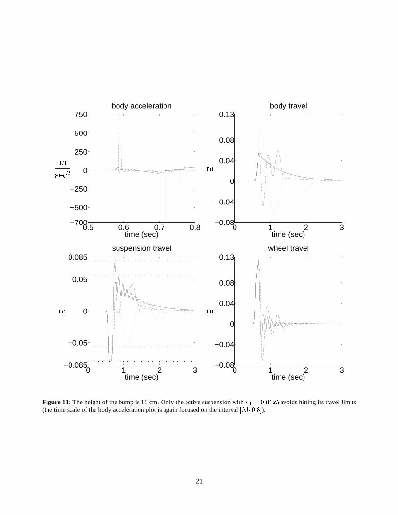
3. Fig. 11 is witha = 0:055 m (road bump height 11 cm).

In Fig. 9, where none of the three configurations hits the suspension travel limits, we can see the improve-ment of ride quality achieved by the active suspension: the body acceleration is reduced by almost 70% and thebody travel by almost 80% compared to the passive suspension. However, the suspension travel is increasedslightly for the active designs. Note that sincej�j � m1 throughout this simulation, the two active designsbehave in an identical manner and therefore their plots overlap.

As the height of the road bump is increased in Fig. 10, the active suspension with�1 = 0 becomes the firstone to hit its travel limits. As a result, a very large acceleration is transmitted to the car body. The activesuspension with�1 = 0:0125 does not hit its travel limits, but it still generates a slightly larger accelerationthan the passive suspension aroundt = 0:6 sec. This is due to the fact that in the first part of the simulationthis configuration isolated its passengers much better thanthe passive one, yet still managed to avoid hitting itstravel limits; this can only be achieved by generating a slightly larger acceleration as soon as the suspensiontravel exceeds5:5 cm, causing the control objective to shift from the regulation of the car body displacementx1 to the regulation of the suspension travel�.

A further increase in the height of the road bump causes both the passive and the active suspension with�1 = 0 to hit their travel limits in Fig. 11, generating very large car body accelerations. The active design with�1 = 0:0125 is the only one which does not hit its travel limits and results in accelerations that are significantlysmaller than for the other two configurations.

18

0 1 2 3−4

−2

0

2

4

5

time (sec)

body acceleration

0 1 2 3−0.02

0

0.02

0.04

0.06

0.07body travel

time (sec)

0 1 2 3−0.085

−0.05

0

0.05

0.085

time (sec)

suspension travel

0 1 2 3−0.02

0

0.02

0.04

0.06

0.07

time (sec)

wheel travel

msec2

m

m

mFigure 9: The height of the bump is 5 cm. None of the three configurations hitsthe suspension travel limits (note that thedashed and solid lines overlap).

19

0.5 0.6 0.7 0.8−30

0

50

100

150

time (sec)

body acceleration

0 1 2 3−0.03

0

0.03

0.06

0.09body travel

time (sec)

0 1 2 3−0.085

−0.05

0

0.05

0.085

time (sec)

suspension travel

0 1 2 3−0.03

0

0.03

0.06

0.09

time (sec)

wheel travel

msec2

m

m

mFigure 10: The height of the bump is 7.6 cm. Only the active suspension with�1 = 0 hits its travel limits (note thedifferent time scale of the body acceleration plot).

20

0.5 0.6 0.7 0.8−700

−500

−250

0

250

500

750

time (sec)

body acceleration

0 1 2 3−0.08

−0.04

0

0.04

0.08

0.13body travel

time (sec)

0 1 2 3−0.085

−0.05

0

0.05

0.085

time (sec)

suspension travel

0 1 2 3−0.08

−0.04

0

0.04

0.08

0.13

time (sec)

wheel travel

msec2

m

m

mFigure 11: The height of the bump is 11 cm. Only the active suspension with�1 = 0:0125 avoids hitting its travel limits(the time scale of the body acceleration plot is again focused on the interval[0:5 0:8]).

21

CONCLUDING REMARKS

Backstepping designs feature significant flexibility, which can be used to successfully resolve many of thetradeoffs inherent in real-world control applications. Inthis paper we demonstrated this capability for activesuspension systems: the introduction of a nonlinear control objective allowed us to successfully negotiate andimprove the fundamental tradeoff between ride quality and suspension travel.

There are several issues related to this design that need further investigation. A critical one is the sensitivityof the response to measurement errors and uncertainty in theplant parameters. Here we designed a full-statefeedback controller, thus assuming the availability of position and velocity measurements for both the carbody and the wheel (x1; : : : ; x4), as well as actuator pressure (x5) and valve position (x6). In real activesuspension designs, the last two signals are usually measured; the first four, however, are estimated from directmeasurements of body acceleration, suspension travel, andpossibly wheel acceleration. Clearly, the estimationprocess can introduce bias and errors in addition to the noise included in the original measurements. Theclosed-loop stability properties achieved with our controller guarantee its robustness to small measurementand estimation errors, but further research is required to determine how small the errors have to be. As foruncertainty in the plant parameters, our first results reported in [11] indicate that our controller is quite robustto variations in many plant parameters; adaptation of a single gain is enough to robustify the controller againstuncertainty in the remaining parameters. Another important issue is the choice of the critical nonlinear filterparameters�0, m1 and�1, which specify how soft the suspension is when its travel is small, how soon thenonlinearity starts stiffening the suspension, and how fast it stiffens it. The main advantage of employing anactive suspension is the associated adaptation potential:the suspension characteristics can be adjusted whiledriving, to match the profile of the road being traversed. Theeffective and efficient adaptation of the nonlinearfilter parameters can realize this potential.

APPENDIX

The backstepping design procedure for our nonlinear activesuspension controller begins with the choice ofregulated variable defined by (50), (41) and (42), and is now presented in detail:

Step 1: The derivative ofz1 is_z1 = _x1 � _�x3= x2 + (�0 + �1'(�))(�x3 � x3)= x2 + (�0 + �1'(�))(x1 � z1 � x3)= z2 + �1 + (�0 + �1'(�))� � (�0 + �1'(�))z1 : (65)

The choice of the first stabilizing function�1 = �c1z1 � (�0 + �1'(�))� ; (66)

yields _z1 = �c1z1 � (�0 + �1'(�))z1 + z2 : (67)

Step 2: The derivative ofz2 is computed as_z2 = _x2 � _�1= � 1Mb [Ka(x1 � x3) + Ca(x2 � x4)� A� ( z3 + �2| {z }�x5 )] + g2 ; (68)

22

where g2 = � _�1= c1[�c1z1 � (�0 + �1'(�))z1 + z2]+ (�0 + �1'(�))(x2 � x4) + �1 d'd� (x2 � x4)� :We choose the second stabilizing function�2 as�2 = �MbA ��c2z2 � z1 + 1Mb [Ka(x1 � x3) + Ca(x2 � x4)]� g2� ; (69)

so (68) becomes _z2 = �c2z2 � z1 + A�Mb z3 : (70)

Step 3: The derivative ofz3 is_z3 = _�x5 � _�2= ���x5 � ��A(x2 � x4) + � ( z4 + �3| {z }x6w3 ) + g3 + (d3 + n3h3)r ; (71)

wherew3 is defined by (49),n3 = �MbKtAMus andd3 = n3( CaMb � �0)h3 = ��1'(�)� �1d'd� �g3 = ��MbA ��(c2 + c1)(�c2z2 � z1 + A�Mb z3) + c1�1 d'd� (x2 � x4)z1+ [c21 � 1 + c1(�0 + �1'(�))][�c1z1 � (�0 + �1'(�))z1 + z2]+ 1Mb [Ka(x2 � x4) + Caw1]� (�0 + �1'(�))w1� 2�1 d'd� (x2 � x4)2 � �1 d2'd�2 (x2 � x4)2� � �1 d'd� w1�#w1 = �mt[Ka(x1 � x3) + Ca(x2 � x4)�Ax5] + KtMusx3 �= _x2 � _x4 + KtMus r�mt = 1Mb + 1Mus :With the choice of the third stabilizing function�3 = 1� ��c3z3 � A�Mb z2 � b3h23z3 + ��x5 + ��A(x2 � x4)� g3� ; (72)

(71) becomes _z3 = �c3z3 � A�Mb z2 + � z4 + d3r + n3h3r � b3h23z3 : (73)

23

Step 4: The derivative ofz4 is computed as_z4 = ddt(x6w3)� _�3= 1� (�x6 + u)w3 � 12jw3j jx6jw2 + g4 + (d4 + n4h4)r ; (74)

wheren4 = n3 = �MbKtAMus andw2 = ��x5 � �A(x2 � x4) + x6w3 �= 1� _�x5 = _x5 �d4 = (c3 + c2 + c1) d3� + Kt AMus (�A2 +Ka �mtC2a + �0mtCaMb)h4 = 1� (c3 + c2 + c1 + b3h23)h3 + 1� b3h23( CaMb � �0)� 1� "2�1 d2'd�2 (x2 � x4)� �mtCa�1d'd� �� c1�1 d'd� z1 �mtCa�1'(�) + 4�1 d'd� (x2 � x4)�g4 = � 1� ��(c3 + c2 + c1 + b3h23)(�c3z3 � A�Mb z2 + � z4 � b3h23z3)� A�Mb �z2 + ��w2 + ��Aw1 � 2b3z3h3�h3 + �g4��g4 = �MbA "�(c2 + c1)(�c2�z2 � �z1) + c1�1 d2'd�2 (x2 � x4)2z1+ c1�1 d'd� w1z1 + 2c1�1 d'd� (x2 � x4)�z1+ [c21 � 1 + c1(�0 + �1'(�))]z1 + 1Mb (Kaw1 + Ca �w1)� 6�1 d'd� (x2 � x4)w1 � (�0 + �1'(�)) �w1 � 3�1 d2'd�2 (x2 � x4)3� �1 d3'd�3 (x2 � x4)3� � 3�1 d2'd�2 (x2 � x4)w1� � �1 d'd� �w1�#�h3 = _h3 = �2�1 d'd� (x2 � x4)� �1d2'd�2 (x2 � x4)��z2 = _z2 = �c2z2 � z1 + A�Mb z3�z1 = _z1 = �c1z1 � (�0 + �1'(�))z1 + z2z1 = _�z1 = �(c1 + �0 + �1'(�))�z1 � �1 d'd� (x2 � x4)z1 + �z2�w1 = �mt[Ka(x2 � x4) +Caw1 �Aw2] + KtMusx4 �= _w1 �mtCa KtMus r� :The resulting control lawu is chosen as u = �w3�4 ; (75)

24

with the last stabilizing function�4 = �c4z4 � � z3 � b4h24z4 + 1� x6w3 + 12jw3j jx6jw2 � g4 : (76)

Hence, (74) becomes _z4 = �c4z4 � � z3 + d4r + n4h4r � b4h24z4 : (77)

REFERENCES

[1] W. R. Anderson,Controlling Electrohydraulic Systems, New York, NY: Marcel Dekker, 1988.

[2] A. Alleyne and J. K. Hedrick, “Nonlinear control of a quarter car active suspension,”Proceedings of the1992 American Control Conference, Chicago IL, pp. 21–25.

[3] A. Alleyne, P. D. Neuhaus, and J. K. Hedrick, “Application of nonlinear control theory to electronicallycontrolled suspensions,”Vehicle System Dynamics, vol. 22, pp. 309–320, 1993.

[4] J. K. Hedrick and T. Butsuen, “Invariant properties of automotive suspensions,”Proceedings of the Insti-tution of Mechanical Engineers, vol. 204, pp. 21–27, 1990.

[5] D. Hrovat, “Influence of unsprung weight on vehicle ride quality,” Journal of Sound and Vibration,vol. 124, pp. 497–516, 1988.

[6] D. Hrovat, “Optimal active suspension structures for quarter-car vehicle models,”Automatica, vol. 26,pp. 845–860, 1990.

[7] D. Hrovat, “Applications of optimal control to advancedautomotive suspension design,”Transactions ofthe ASME, Journal of Dynamic Systems, Measurement and Control, vol. 115, pp. 328–342, 1993.

[8] I. Kanellakopoulos, P. V. Kokotovic, and A. S. Morse, “Atoolkit for nonlinear feedback design,”Systems& Control Letters, vol. 18, pp. 83–92, 1992.

[9] D. Karnopp, “Theoretical limitations in active vehiclesuspensions,”Vehicle System Dynamics, vol. 15,pp. 41–54, 1986.

[10] M. Krstic, I. Kanellakopoulos, and P. V. Kokotovic,Nonlinear and Adaptive Control Design, New York,NY: John Wiley & Sons, 1995.

[11] J.-S. Lin and I. Kanellakopoulos, “Adaptive nonlinearcontrol in active suspensions,”Proceedings ofthe 13th World Congress of International Federation of Automatic Control, San Francisco, CA, vol. F,pp. 341–346, 1996.

[12] H. E. Merritt, Hydraulic Control Systems, New York, NY: John Wiley & Sons, 1967.

[13] L. R. Ray, “Robust linear-optimal control laws for active suspension systems,”Transactions of the ASME,Journal of Dynamic Systems, Measurement and Control, vol. 114, pp. 592–598, 1992.

[14] M. Satoh, N. Fukushima, Y. Akatsu, I. Fujimura, and K. Fukuyama, “An active suspension employingan electrohydraulic pressure control system,”Proceedings of the 29th IEEE Conference on Decision andControl, Honolulu, HI, pp. 2226–2231, 1990.

25

[15] M. Sunwoo and K. C. Cheok, “An application of explicit self-tuning controller to vehicle active sus-pension systems,”Proceedings of the 29th IEEE Conference on Decision and Control, Honolulu, HI,pp. 2251–2257, 1990.

[16] A. G. Thompson, “Design of active suspensions,”Proceedings of the Institution of Mechanical Engineers,vol. 185 (part 1), pp. 553–563, 1970–71.

[17] A. G. Thompson, “An active suspension with optimal linear state feedback,”Vehicle System Dynamics,vol. 5, pp. 187–203, 1976.

[18] A. G. Thompson, “Optimal and suboptimal linear active suspensions for road vehicles,”Vehicle SystemDynamics, vol. 13, pp. 61–72, 1984.

[19] R. B. Walters,Hydraulic and Electro-Hydraulic Control Systems, New York, NY: Elsevier Science, 1991.

[20] C. Yue, T. Butsuen and J. K. Hedrick, “Alternative control laws for automotive active suspensions,”Transactions of the ASME, Journal of Dynamic Systems, Measurement and Control, vol. 111, pp. 286–291, 1989.

26