Embed Size (px)
Citation preview

THEORETICAL FUNDAMENTALS OF ELECTRICAL ENGINEERING 2
Methodological guidelines and assignments for laboratory works
for the 5B071800 – “Electrical power engineering” baccalaureate specialty students
Almaty 2017
Noncommercial
joint stock
company
ALMATY
UNIVERSITY OF
POWER
ENGINEERING &
TELECOMMUNICATIONS
Department of Theoretical
electrical engineering

2
AUTHORS: A. S. Baimaganov, S. J. Kreslina. Theoretical fundamentals of
electrical engineering 2. Methodological guidelines and assignments for laboratory
works for the 5B071800 – “Electrical power engineering” baccalaureate specialty
students. – Almaty: AUPET, 2017. – 30 p.
Methodological guidelines and assignments for preparing, execution and de-
sign of laboratory works on “Theoretical fundamentals of electrical engineering 2”
discipline are provided.
Each laboratory work includes the following sections: the purpose of the
work, preparation for a laboratory work, procedure of carrying out the work, pro-
cessing the results of experiments and methodological guidelines.
Methodological guidelines and assignments are intended for second-year stu-
dents, who are educated in English language on 5B071800 – “Electrical power en-
gineering” baccalaureate specialty.
13 illustrations, 15 tables, 6 items of references.
Reviewer: PhD B. I. Tuzelbayev
It is printed according to the publishing plan of non-commercial JSC “Almaty
university of power engineering & telecommunications” for 2017 y.
© NJSC “Almaty university of power engineering & telecommunications”, 2017 y.

3
2017 y. publishing plan, 35 position
Aliaskar Baimaganov
Svetlana Kreslina
THEORETICAL FUNDAMENTALS OF ELECTRICAL ENGINEERING 2
Methodological guidelines and assignments for laboratory works
for the 5B071800 – “Electrical power engineering” baccalaureate specialty students
Editor Y. R. Gabdulina
Standard expert N. K. Moldabekova
Signed to publication _____________ Layout size 60×84 1/16
Printed 50 copies Printout paper № 1
Volume 1.8 edu.-pub. sheet Order ____ Price 900 tenge
Copying service
Non-commercial joint stock company
“Almaty university of power engineering & telecommunications”
126, Baitursinov Street, Almaty, 050013

4
Contents
Introduction ....................................................................................................... 5
Requirements for the registration of report on laboratory work ....................... 7
1 Laboratory work №1. Research of transients in the first order linear
electric circuits ............................................................................................................ 9
2 Laboratory work №2. Research of transients in the second order linear
electric circuits .......................................................................................................... 13
3 Laboratory work № 3. Research of K-type passive filters ........................... 16
4 Laboratory work № 4. Research of various operating modes of the
transmission lines ...................................................................................................... 22
5 Laboratory work № 5. Research of various operating modes of the
lossless homogeneous line ........................................................................................ 26
References ....................................................................................................... 31

5
Introduction
The laboratory research are of great importance for the quality of training and
formation of students’ creative thinking and engineering skills. The performance of
laboratory works allows students to apply theoretical principles in practical calcula-
tions in order to obtain skills of independent analysis of electrical circuits, which
ultimately contributes to the successful mastery of the discipline.
The manual contains a description of the mandatory laboratory works on
“Theoretical fundamentals of electrical engineering 2” (TFEE2) discipline for the
5B071800 – “Electrical power engineering” baccalaureate specialty.
Laboratory work is a complex of experimental and theoretical assignments in
the study of linear electric circuits of direct, single-phase and three-phase sinusoidal
current. All laboratory work is performed by the front way after the respective top-
ics in the lecture material is presented.
The practical implementation of the laboratory researches at the “Theoretical
electrical engineering” department provides by using of the “UILS-2” – universal
teaching and research laboratory workbenches. The “UILS-2” workbench is fixed
on the table and is a metal box that consist of active and passive units and a
patchbay for the assembly of electrical circuits to carry out the experiment. The
workbench also includes 29 external components (resistors, capacitors and induc-
tors) and a set of connecting leads with plugs.
Active blocks are located in the left side of the stand and consist of a block of
DC voltage sources and blocks of the single- and three-phase sinewave voltage
sources. Passive units are located in the right side of the stand and consist of a block
of a variable resistance and blocks of a variable inductance and a variable capaci-
tance. A patchbay is located at the center of the stand.
The DC voltage unit comprises:
- an adjustable DC stabilized voltage source with regulation range from 0.25
to 24 V;
- an unregulated DC voltage source with output voltage of about 20 V;
- “electronic switch” used to study transients.
Both DC voltage sources are provided with an electronic protection circuit
against short-circuits and overloads. The current of protection activation is 1 A.
AC unit is a functional generator with adjustable frequency and value of volt-
age of sinusoidal, rectangular and triangular shapes.
The unit is provided with an electronic protection circuit against short-circuits
and overloads. The current of protection activation is 1 A.
The three-phase voltage unit is a source of three-phase voltage of commercial
frequency f = 50 Hz. Source contains three electrically independent from each other
phases.
Each phase is equipped with an electronic protection against short-circuits
and overloads. The current of protection activation is 1 A.

6
The unit of variable resistors consists of three unregulated resistors R1, R2, R3
and an adjustable R4. Regulation of value of resistor R4 is performed in the range
from 0 to 999 Ω a stepwise in increments of 1 Ω by using three switches: the hun-
dreds (0 ... 9), the tens (0 ... 9) and the units (0 ... 9) Ω.
The unit of variable inductance includes three unregulated inductors L1, L2, L3
and an adjustable inductor L4. Regulation of inductance L4 can be adjusted between
0 and 99.9 mH in steps of 0.1 mH by using three switches: the tens (0 ... 9), the
units (0 ... 9) and the tenths (0 ... 9) mH.
The unit of variable capacitance consists of three unregulated capacitors C1,
C2, C3 and an adjustable C4. Regulation of capacitance C4 is carried out in the range
from 0 to 9.99μF in steps of 0.01 μF using three switches: the units (0 ... 9), the
tenths (0 ... 9) and the hundredths of (0 ... 9) μF.
On the front panel of the blocks are located: the light indicators (LEDs, light
indicators), the controls (knobs switches, toggle switches, and buttons) and meas-
urement devices.
A patchbay is a panel with 67 pairs connected with each other of jacks for
plugging and mounting the components of studied electrical circuits
The external elements are designed as the transparent plastic boxes, in which
there are plugs to connect and soldering inside the elements of electric circuits: R, L
and C.
It is necessary to switch the toggle switch “POWER” in “ON” position to turn
on the active unit, at the same time on front panel the “POWER LED” lights.
Measuring devices of the units are designed to display the value of current
and voltage of regulated sources. Regulation performed by means of potentiometer
handle.
The frequency is adjusted stepwise with 1 kHz step by a switch and smoothly
by a “FREQUENCY SMOOTHLY” potentiometer. When the potentiometer is at
the right position, the frequency of the output voltage corresponds to the value indi-
cated on the stepwise switch with an accuracy of ± 2%.
The voltage of each phase at the output of unit of the three-phase voltage
source can be adjusted stepwise from 0 to 30 V in increments 1 V via two switches:
tens (0 ... 3) and units (0 ... 9) of Volts.
In the event of a short circuit or an overload in the power supply units an
electronic protection is activated, and “PROTECTION” indicator lights. After re-
moving the causes of a short circuit or overload, it is necessary to return the power
supply unit in operating state by pressing “PROTECTION” button upon that the in-
dicator goes out.

7
Requirements for the registration of report on laboratory work
The assignment for the current laboratory work the student gets in advance on
the previous lesson, for one or two weeks earlier.
Each student prepares a report himself in order to carry out laboratory work,
acquainted with the purpose of work and with the basic theoretical principles used
in the experiment.
Before implementation of experimental part, the student is interviewed on the
preparation for a laboratory work, shows the prepared report for the execution of
laboratory work to the teacher and gets the admission to the work.
After executing the experimental part, the report is finalized: a comparison
between theory and experiment is carried out, the necessary graphs are plotted, an
analysis the results are carried out and conclusions on the work are made.
Each student defends the report on laboratory work individually at the current
or following laboratory classes, or at the consultations.
The report should contain the title page and the following sections:
- purpose of the work;
- basic theoretical principles and answers to questions of preparation for a
laboratory work;
- brief information about the experiment;
- the scheme of analyzed electric circuit;
- the formulas, and the results of theoretical calculations for specific modes
of the electric circuit;
- results of the study: tables, graphs, diagrams, numerical values of the cir-
cuit parameters, electric currents and voltages, etc.;
- the conclusions of the work done.
See the template of the title page on the next page.
Reports should be performed only on a one side of white sheet or of lined pa-
per with size of A4 (210x297mm). The text should be written neatly. When writing
the text is permitted to use only generally accepted abbreviations or designations,
decrypted at the first mention.
Student is allowed to the next laboratory work if he has executed and defend-
ed a previous laboratory work.
8
Non-commercial joint stock Company
ALMATY UNIVERSITY OF POWER ENGINEERING & TELECOMMUNICATIONS
Department of “Theoretical electrical engineering”
R E P O R T
on laboratory work № ____
on the “Theoretical fundamentals of electrical engineering 2” discipline
__________________________________________________________________ (Title of the laboratory work)
__________________________________________________________________
5B071800 – “Electrical power engineering” baccalaureate specialty
Done by __________________________________ Group _____________ (Student’s Surname & Initials) (Academic group code)
Checked by ____________________________________________________ (Teacher’s academic degree, academic rank, Surname & Initials)
____________ ___________________ «____» ________________20___ y. (Score) (Teacher’s signature) (Date)

9
Almaty 20___ y.
1 Laboratory work №1. Research of transients in the first order linear
electric circuits
Purpose is obtaining the skills of experimental research of transients in the
first order linear electrical circuits with a single energy storage element.
1.1 Preparation for a laboratory work
Repeat section “Transients in the first order linear electric circuits” of TFEE2
discipline.
Answer the questions in writing and do the following assignments:
1) What is the transient process, and what are its causes? In which of electri-
cal circuits can occur transients?
2) Write down the commutation laws.
3) What are named as steady and free components of the transient time func-
tion, for example, of the current or of the voltage?
4) What is the physical sense of the time constant of the circuit? What is the
values of RC- and RL-circuit time constant?
5) What is named as damping factor of the circuit, logarithmic decrement?
6) Write down the expressions of instantaneous values of uC(t) and iC(t) at
short circuit of RC - network, plot the graphs of uC(t) and iC(t).
7) How to determine experimentally the time constant of the circuit?
8) Write down the expressions of instantaneous values of uL(t), iL(t) for the
circuit in figure 1.2 after the switch is opened and plot their graphs.
1.2 Procedure of carrying out the work
1.2.1 Assemble the electric circuit in figure 1.1.
1.2.2 Set values of the EMF E0, the resistor R and the capacitor C according
to the assignment option, table 1.1. Set value of R1 in the range of 100...300 Ω.
1.2.3 Plug in the voltage of capacitor to the oscilloscope input. Copy in a
scale from the oscilloscope screen or take a screenshot of the voltage curve of uC(t).
1.2.4 Plug in the voltage of resistor R to the oscilloscope input. Copy in a
scale from the oscilloscope screen or take a screenshot of the voltage curve of uR(t).
This curve in the appropriate scale represents the curve of current through the ca-
pacitor:
( )
( ) ( ) RC R
u ti t i t
R .
1.2.5 Change one of the circuit parameters according to assignment option
(table 1.2). Copy in a scale the new curves of uC(t) and uR(t) from the oscilloscope

10
screen or take a screenshots, aligning it with the first curve. Compare the obtained
curves.
1.2.6 Assemble the electric circuit in figure 1.2.
1.2.7 Set values of the EMF E0 and the inductance L (option 1) according to
the assignment option, table 1.3. Set the resistors values of R1 = R = 51 Ω.
1.2.8 Plug in the voltage of resistor R to the oscilloscope input. Copy in a
scale from the oscilloscope screen or take a screenshot of the voltage curve of uR(t).
This curve in the appropriate scale represents the curve of current through the in-
ductor:
( )
( ) ( ) RL R
u ti t i t
R .
1.2.9 Plug in the voltage of inductor to the oscilloscope input. Copy in a scale
from the oscilloscope screen or take a screenshot of the voltage curve of ucoil(t).
1.2.10 Set the new value of inductance (option 2) according to assignment
option (table 1.3). Copy in a scale the new curves of ucoil(t) and uR(t) from the oscil-
loscope screen or take a screenshots, aligning it with the first curve. Compare the
obtained curves.
Figure 1.1 – Scheme for research of transient in RC-circuit

11
Figure 1.2 – Scheme for research of transient in RL-circuit
Table 1.1 – Parameters of RC-circuit (option 1)
Option E0, V R, Ω С, μF
1 10 300 4
2 15 400 2
3 20 200 5
4 10 600 5
5 15 500 3
Table 1.2 – Parameters of RC - circuit (option 2)
Option E0, V R, Ω С, μF
1 10 600 4
2 15 400 4
3 20 400 5
4 10 300 5
5 15 500 6
Table 1.3 – Parameters of RL - circuit
Option E0, V L, mH (option 1) L, mH (option 2)
1 10 100 50
2 12 45 90
3 15 80 40
4 10 35 70
5 15 94 47

12
1.3 Processing the results of experiments
1.3.1 Calculate the time constants τ and damping factors α of the circuit
shown in figure 1.1 for two given options of the circuit parameters (tables 1.1 and
1.2.): τRС1, RС1 и τRС2, RС2.
1.3.2 Determine the time constant τRС and the damping factor RС of the RC-
circuit in figure 1.1 by the images of the voltage curves across the capacitor of uC(t)
for two given options of the circuit parameters (points 1.2.3 and 1.2.5).
1.3.3 Theoretically calculate voltage time function of uC(t) by the known pa-
rameters of the circuit according to assignment option (table 1.1).
1.3.4 Plot graphs of the calculated and experimental curves of uC(t) on the
same figure.
1.3.5 Calculate the time constants τ and damping factors α of the circuit
shown in figure 1.2 for two given options of the inductance value (table 1.3): τRL1,
RL1 и τRL2, RL2. It is necessary to take into account of RCoil – the resistance of the
inductor, then the total resistance of the circuit will be of R = R1 + R + Rcoil.
1.3.6 Determine the time constant τRL and the damping factor RL of the RL -
circuit in figure 1.2 by the images of the voltage curves across the resistor R of uR(t)
for two given options of the inductance (points 1.2.8 and 1.2.10).
1.3.7 Theoretically calculate a current of iL(t) and a voltage of ucoil(t) time
function by the known parameters of the RL – circuit in figure 1.2 according to as-
signment option (table 1.3).
1.3.8 Plot graphs of the calculated and experimental curves of iL(t) and ucoil(t)
on the same figure.
1.3.9 Make a conclusion about the impact of the value of resistance R or ca-
pacitance C on the time constant τ of the circuit and consequently on the rate of
transient process, determine the time of discharge of the capacitor. In addition, ana-
lyze the impact of the value of the inductance L on the time constant τRL of the RL -
circuit and, accordingly, on the rate of the transient process.
1.4 Methodological guidelines
The scale of the time axis is determined from the condition that the electronic
switch (S) commutes with a frequency f = 50 Hz and a period of T = 20 ms. The
first half of the period (10 ms), the electronic switch is opened, the capacitor is
charged. The second half of the period (10 ms), the electronic switch is closed, the
capacitor discharges.
The time constant of the RC-circuit RC is determined by experimental curve
of uC(t) as a subtangent (figure 1.3).
The time constant of the RL-circuit τRL is defined by the same way using
curve of uR(t).

13
Figure 1.3 – Determination the time constant RC of RC-circuit
2 Laboratory work №2. Research of transients in the second order linear
electric circuits
Purpose is obtaining the skills of experimental research of transients in an
electrical circuit with two energy storage elements – with inductor and capacitor.
2.1 Preparation for a laboratory work
Repeat section “Transients in the second order linear electric circuits” of
TBEE2 discipline.
Answer the questions in writing and do the following assignments:
1) Write down the equation by Kirchhoff's voltage law (KVL) for the free
components of voltages across elements of RLC - circuit and the corresponding
characteristic equation of the circuit.
2) Which roots of the characteristic equation of RLC - circuit corresponds to
the overdamped character of discharge of the capacitor? Write down the expressions
for the instantaneous values of the uC(t), i(t) and uL(t) at overdamped character of
the capacitor discharge. Draw graphs of these time functions.
3) Which roots of the characteristic equation of RLC - circuit corresponds to
the critical overdamped character of discharge of the capacitor? Write down the ex-
pressions for the instantaneous values of the uC(t), i(t) and uL(t) at critical
overdamped character of the capacitor discharge.
4) Write down the expression for the calculation of the critical resistance of
RLC - circuit.
5) What is called logarithmic damping decrement?

14
6) Which roots of the characteristic equation of RLC - circuit corresponds to
the underdamped character of the capacitor discharge? Write down the expressions
for the instantaneous values of the uC(t), i(t) and uL(t) at underdamped character of
discharge of the capacitor. Draw graphs of these time functions.
7) How to determine the attenuation coefficient α and the natural oscillation
frequency ω0 of the circuit both by theoretical calculation and by experimental way
(according to the voltage curve)? How do these values depend on R, L and C?
2.2 Procedure of carrying out the work
2.2.1 Assemble the electric circuit as shown in figure 2.1.
2.2.2 Set values of the resistor R, the inductor L and the capacitor C according
to the assignment option, table 2.1. Measure the coil resistance Rcoil. Set values of
the R1 in the range of 100...300 Ω and of the EMF E0 = 15…20 V.
2.2.3 Plug in the voltage from the capacitor to the oscilloscope input. Re-
search the oscillation discharge of a capacitor, copy the voltage curve of uC(t) in a
scale from the oscilloscope screen or take a screenshot.
2.2.4 Plug in the voltages of uR(t) and uL(t) to the input of the oscilloscope
and copy the oscillogram of these voltages at the underdamped character of the ca-
pacitor discharge.
2.2.5 By increasing the resistance of the resistor R to achieve the disappear-
ance of fluctuations on the voltage curve of uC(t) that corresponds to the critical
overdamped character of the capacitor discharge. Write down the value of obtained
critical resistance Rcr.exp. of circuit with taking into account the coil resistance Rcoil.
Compare the value of critical resistance obtained in the experiment with the calcu-
lated. Copy in a scale the voltage curve of uC(t) from the oscilloscope screen or take
a screenshot.
2.2.6 Enlarge total resistance of the circuit RΣ in two times in comparison
with the critical. Copy in a scale the obtained voltage curves of uC(t), uL(t) and uR(t)
from the oscilloscope screen for the overdamped character of the capacitor dis-
charge.
Figure 2.1 – Scheme of research the RLC-circuit

15
Table 2.1
Option R, Ω L, mH С, μF
1 1 10 4
2 1 20 3
3 1 20 2
4 1 15 2
5 1 10 3
2.3 Processing the results of experiments
2.3.1 For the circuit in figure 2.1 theoretically calculate the damping factor
αtheory. and the natural frequency ω0theory by using given values of total resistance RΣ
= R + Rcoil, L and C (according to the assignment option, table 2.1.
2.3.2 Calculate the experimental values of the damping factor αexp. and the
natural frequency ω0exp. of the circuit by using the experimentally obtained image of
voltage waveform across the capacitor uC(t) (see point 2.2.3).
2.3.3 Theoretically calculate the critical resistance Rcr.theory of the circuit.
2.3.4 Make conclusions on the done work: compare the theoretically calculat-
ed values of , 0 and Rcr with ones obtained experimentally. Analyze the impact
of the total resistance of the circuit on the character of discharge of the capacitor.
2.4 Methodological guidelines
The scale of the time axis is determined from the condition that the electronic
switch (S) commutes with a frequency f = 50 Hz and a period of T = 20 ms. The
first half of the period (10 ms), the electronic switch is opened, the capacitor is
charged. The second half of the period (10 ms), the electronic switch is closed, the
capacitor discharges.
Theoretical values of the damping factor theory, the natural frequency 0theory
and the critical resistance Rcr.theory are determined by the formulas: 2
0 .
1; ; 2 .
2 2theory theory cr theory
R R LR
L LC L C
The experimental values of the damping factor αtheory. and the natural frequen-
cy ω0theory are determined by the voltage curve uC(t) which obtained from the oscil-
loscope screen, as shown in figure 2.2.

16
Figure 2.2 – Determination the exp., T0 and 0theory of RLC-circuit
The natural frequency 0theory can be calculated by the formula:
0 0
0
22 f
Т
,
where T0 is period of free oscillations is determined by the voltage curve uC(t)
as shown in figure 2.2.
The experimental value of the damping factor exp. can be calculated by the
logarithmic decrement and period of natural oscillation by the formula:
1exp.
0 1 0
1 ( )
( )
c
c
u tп
T u t Т
,
where uC(t1) = E0 – amplitude of the voltage oscillation across capacitor at the
moment t1 = 0. In denominator the value of amplitude of the voltage oscillations
across capacitor after the period T0.
3 Laboratory work № 3. Research of K-type passive filters
Purpose is to research the frequency characteristics of the attenuation coeffi-
cient “a“ and the phase coefficient “b“ for the simplest low-pass (LPF) and high-
pass (HPF) filters.
3.1 Preparation for the laboratory work
Repeat the section “K-type passive filters” of TFEE2 discipline.
Answer the questions in written form and do the following assignments:
1) Give the filter classification.
2) Give the concepts of low-pass, high- pass, band-pass and band-stop fil-
ters.

17
3) Give the definition of the secondary filter parameters. What units they are
measured in?
4) What is the passband and the attenuation band or stopband of an ideal fil-
ter?
5) What is the matched operation mode of filter?
6) Draw the π – section and the T – section schemes of low-pass filter.
7) Draw the π – section and the T – section schemes of high-pass filter.
8) Draw the graphs of frequency dependences of attenuation a(f) and phase
b(f) coefficients for the LPF.
9) Draw the graphs of frequency dependences of attenuation a(f) and phase
b(f) coefficients for the HPF.
10) Write down the calculation formulas of cutoff frequency fcut and charac-
teristic resistance ρ for the LPF.
11) Write down the calculation formulas of cutoff frequency fcut and charac-
teristic resistance ρ for the HPF.
12) Choose the filter scheme and the elements parameters of filter according
to option (table 3.1).
13) Calculate the cutoff frequency fcut and characteristic resistance ρ for the
chosen filter parameters. Write down the calculation results in table 3.2.
3.2 Procedure of carrying out the work
3.2.1 Assemble the circuit shown in figure 3.1. Use the chosen scheme of re-
searched filter according to assignment option (table 3.1.).
Table 3.1 – Assignment options for the laboratory work
Option Filter type Filter circuit U1, V L, mH С, μF
1 LPF T – section 5 80 0.5
2 HPF T – section 4 70 0.4
3 LPF π – section 3 60 0.6
4 HPF π – section 4 50 0.7
5 LPF T – section 5 40 0.3
3.2.2 Set the values of U1, L, C, Rload = ρ according to option (table 3.1.).
3.2.3 Measure the RMS values of output voltage U2 across points 2 – 2' and
the time phase shift Т2 – Т1 between the input u1(t) and the output u2(t) voltages for
various values of frequency. Change the frequency f of the generator, multiplying
by the corresponding coefficient to the cutoff frequency (12 values), using the table
3.3 for LPF or the table 3.4 for HPF. The voltage across the input of filter U1 should
be kept constant. Write down the measurement results in table 3.2.
Table 3.2 – Frequency characteristics of the attenuation a and phase b coefficients
fcut = ; Rload = ; U1 = ; L = ; C = .

18
f, Hz U2, V T2 – T1, s a, Np b, deg.
f1
…
f12
Low-pass filters
Π-section scheme of low-pass filter
T-section scheme of low-pass filter
Figure 3.1 – Schemes of low-pass filters
High-pass filters
Π-section scheme of high-pass filter.

19
T-section scheme of high-pass filter
Figure 3.2 – Schemes of high-pass filters
3.3 Processing the results of experiments
3.3.1 Calculate the attenuation coefficients a (f) and the phase coefficients b
(f) for each of frequency values. Write down the calculation results in table 3.2.
3.3.2 Draw the frequency dependence graph of attenuation coefficient а(f) us-
ing an experimental data from the table 3.2, aligning it with the theoretical graph
а(f), which is drew using data from the table 3.3 for LPF or the table 3.4 for HPF.
3.3.3 Draw the frequency dependence graph of phase coefficient b(f) using an
experimental data from the table 3.2, aligning it with the theoretical graph b(f),
which is drew using data from the table 3.3 for LPF or the table 3.4 for HPF.
3.3.4 Compare the theoretical graphs of а(f) and b(f) with those experimental
and explain their differences. Analyze the dependencies of а(f) and b(f) in the pass-
band and the attenuation band. Make the conclusions on the work done.
Table 3.3 – Theoretical dependences of attenuation and phase coefficients of LPF

20
f/f0 0.20 0.40 0.50 0.60 0.70 0.80 1.00 1.10 1.20 1.50 2.00 4.00
а, Np 0 0 0 0 0 0 0 0.90 1.26 1.94 2.74 4.16
b, deg 23 47 60 74 90 106 180 180 180 180 180 180
Table 3.4 – Theoretical dependences of attenuation and phase coefficients of HPF
f/f0 0.25 0.50 0.67 0.83 0.90 1.00 1.25 1.43 1.67 2.00 2.5 5.0
а, Np 4.10 2.74 1.94 1.26 0.90 0 0 0 0 0 0 0
b, deg -180 -180 -180 -180 -180 -180 -106 -90 -74 -60 -47 -23
3.4 Methodological guideline
3.4.1 Relation between complex RMS values of input U1 and output U2 volt-
ages at the match load of filter can be written as follow:
1
2
c a jbUe e e
U
.
Attenuation coefficient is determined by the formula:
2
1
U
Unа ,
and the phase shift coefficient b = u1 – u2, where u1 and u2 – the initial
phases, respectively, of the input and the output voltages.
3.4.2 Cutoff frequency fcut of the LPF is defined by formula:
2 1
; .2
cutcut cutf
L C LC
And the cutoff frequency fcut of the HPF is defined by formula:
1 1
; .22 4
cutcut cutf
L C LC
The load resistance Rload and the internal resistance of generator is taken equal
to the characteristic resistance:
.load in
LR R
C

21
3.4.3 Phase coefficient is determined by the phase time shift Т2-Т1 between
the similar phases of the input u1(t) and the output u2(t) voltages by the formula:
1 2 2 1360 ( )u ub f T T .
The measuring of the initial phase of sinusoidally time-varying voltage is
possible by means of the oscilloscope (figure 3.3).
In order to measure the phase shift between the input and the output voltages
the channel (A) of oscilloscope should be connected to the point (1) (this wire
paints in red color) and the channel (B) – to the point (2) (this wire paints in blue
color). Set the first (red) and the second (blue) survey lines to the same phase point
of the input u1(t) and the output u2(t) voltages, for example in the start zero point of
sinusoidally time-varying function. Read the corresponding time shift interval Δtu2
= Т2 – Т1 between the voltages u1(t) and u2(t) on the third (last) subwindow of the
oscilloscope beneath the main screen. Calculate the phase shift coefficient b by
above formula.
Figure 3.3
22
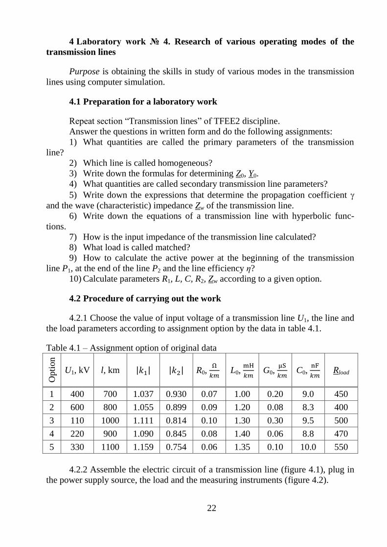
4 Laboratory work № 4. Research of various operating modes of the
transmission lines
Purpose is obtaining the skills in study of various modes in the transmission
lines using computer simulation.
4.1 Preparation for a laboratory work
Repeat section “Transmission lines” of TFEE2 discipline.
Answer the questions in written form and do the following assignments:
1) What quantities are called the primary parameters of the transmission
line?
2) Which line is called homogeneous?
3) Write down the formulas for determining Z0, Y0.
4) What quantities are called secondary transmission line parameters?
5) Write down the expressions that determine the propagation coefficient
and the wave (characteristic) impedance Zw of the transmission line.
6) Write down the equations of a transmission line with hyperbolic func-
tions.
7) How is the input impedance of the transmission line calculated?
8) What load is called matched?
9) How to calculate the active power at the beginning of the transmission
line P1, at the end of the line P2 and the line efficiency η?
10) Calculate parameters R1, L, C, R2, Zw according to a given option.
4.2 Procedure of carrying out the work
4.2.1 Choose the value of input voltage of a transmission line U1, the line and
the load parameters according to assignment option by the data in table 4.1.
Table 4.1 – Assignment option of original data
Opti
on
U1, kV l, km |𝑘1| |𝑘2| R0, Ω
𝑘𝑚 L0,
mH
𝑘𝑚 G0,
μS
𝑘𝑚 C0,
nF
𝑘𝑚 Rload
1 400 700 1.037 0.930 0.07 1.00 0.20 9.0 450
2 600 800 1.055 0.899 0.09 1.20 0.08 8.3 400
3 110 1000 1.111 0.814 0.10 1.30 0.30 9.5 500
4 220 900 1.090 0.845 0.08 1.40 0.06 8.8 470
5 330 1100 1.159 0.754 0.06 1.35 0.10 10.0 550
4.2.2 Assemble the electric circuit of a transmission line (figure 4.1), plug in
the power supply source, the load and the measuring instruments (figure 4.2).

23
4.2.3 Set the given value of supply source voltage U1 at the input of a trans-
mission line, the frequency f = 50 Hz and the precalculated parameters of the equiv-
alent two-port circuit.
Figure 4.1 – Equivalent scheme of the transmission line
Figure 4.2 – Connection diagram for measuring instruments
4.2.4 Set the value of a load resistance Rload according to the option given.
Measure the RMS value of an output voltage of a transmission line U2, the RMS
values of input I1 and output I2 currents of a transmission line. Measure the initial
phase angles of output voltage of a transmission line ψu2 and of the input and the
output currents of a transmission line: ψi1 and ψi2. Write down the obtain results in
table 4.2.
4.2.5 Set the matched load Zload = Zw at the end of a transmission line
(matched load operation mode). Measure the RMS value of output voltage U2, the
RMS values of input I1 and output I2 currents of a transmission line, the initial phase
angle of output voltage ψu2 and the initial phase angles of input ψi1 and output ψi2
currents of a transmission line. Write down the results in table 4.2.
4.2.6 Set a jumper between the output terminals of a transmission line (short-
circuit mode U2=0). Measure the RMS values of input I1 and output I2 currents, the
initial phase angles of input ψi1 and output ψi2 currents of a transmission line. Write
down the results in table 4.2.
4.2.7 Remove jumper from the output terminals of a transmission line (idling
mode I2=0). Measure the RMS values of the output voltage U2 and the input current

24
I1 of a transmission line, the initial phase angles of the output voltage ψu2 and the
input current ψi1 of a transmission line. Write down the results in table 4.2.
Table 4.2 – Determination of initial phase angles of currents and voltages
Operation
mode
U1,
kV
U2,
kV
T2 - T1,
s
ψu2,
deg. I1, A
T2 - T1,
s ψi1, deg. I2, A
T2 - T1,
s
ψi2,
deg.
Load mode
Rload =
Matched load
Zload = Zw
Short-circuit 0 – –
Idling 0 - -
4.3 Processing the results of experiments
4.3.1 Calculate the initial phase angle of output voltage ψu2 and the initial
phase angles of input ψi1 and output ψi2 currents of a transmission line. Write down
the results in table 4.2.
4.3.2 Write down the complex RMS values of the voltages �̇�1, �̇�2 and the
currents 𝐼1̇, 𝐼2̇ for all studied modes in table 4.3.
4.3.3 Calculate the input impedances of a transmission line Z1in, the active
power at the beginning of the transmission line P1, at the end of the line P2 and the
line efficiency η for all researched operation modes by using the experimental data.
Write down the obtain results in table 4.3.
4.3.4 Analyze the results obtained in experiments for various operation mode
of a transmission line. Make the conclusions on the work done.
Table 4.3 – The results of the measurements and calculation
Operation mode Z1in, Ω 𝐼1̇, A �̇�2, kV 𝐼2̇, A P1, kW P2, kW η, %
Load mode
Rload =
Matched load
Zload = Zw
Short-circuit
Idling
25
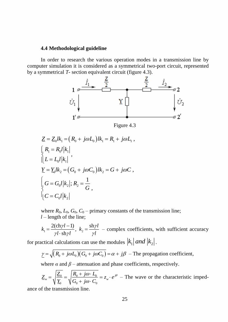
4.4 Methodological guideline
In order to research the various operation modes in a transmission line by
computer simulation it is considered as a symmetrical two-port circuit, represented
by a symmetrical T- section equivalent circuit (figure 4.3).
Figure 4.3
0 1 0 0 1 1 1
1 0 1
0 1
0 2 0 0 2
0 2 2
0 2
,
,
,
1;
,
Z Z lk R j L lk R j L
R R l k
L L l k
Y Y lk G j C lk G j C
G G l k RG
C C l k
where R0, L0, G0, C0 – primary constants of the transmission line;
l – length of the line;
1
2(ch 1)
sh
lk
l l
, 2
sh lk
l
– complex coefficients, with sufficient accuracy
for practical calculations can use the modules 1 2k and k .
0 0 0 0R j L G j C j – The propagation coefficient,
where α and β – attenuation and phase coefficients, respectively.
0 0 0
0 0 0
j
w w
Z R j LZ z e
Y G j C
– The wave or the characteristic imped-
ance of the transmission line.

26
For the measurement and calculation the initial phase angles of voltages and
currents used guidelines for the laboratory work № 3 (see point 3.4.3).
5 Laboratory work № 5. Research of various operating modes of the
lossless homogeneous line
Purpose is obtaining the skills of studying various operating modes of the
lossless homogeneous line by computer simulation.
5.1 Preparation for a laboratory work
Repeat section “Transmission lines. Lossless homogeneous line” of TFEE2
discipline.
Answer the questions in written form and do following:
1) What quantities are called the primary parameters of a lossless line?
2) Which line is called a lossless line?
3) How are secondary parameters of a lossless line determined?
4) Write down the transfer equations of a lossless line.
5) Write down expressions to determine the propagation coefficient and
the wave (characteristic) impedance Zw of a lossless line.
6) What load is called matched load? What is the value of input impedance
of the line with a matched load equaled?
7) At what load in the lossless line is observed a standing wave mode?
8) Write down the equations of input impedance of the lossless line.
9) Calculate Zw, , k1, k2, L, C according to the option (table 5.1). Write
down initial data and calculation results in table 5.2.
10) Calculate currents, voltages for various operation modes of the lossless
line according to a given option (see methodological guidelines). Write down calcu-
lation results in table 5.3 to the “theoretical calculations” row.
Table 5.1 – Assignment options for the laboratory work
Option U1, V f, Hz l, m L0, μH
𝑚 C0,
pF
𝑚 Rload
1 10 108
0.375 1.57 7.10 800
2 15 108
0.500 1.67 6.67 1000
3 20 107
3.750 2.00 5.57 200
4 12 109
0.100 2.50 4.46 400
5 18 108
0.250 1.57 7.10 700
6 25 107
2.500 2.00 5.57 300
Table 5.2 – Parameters of the lossless line

27
U1, V f, Hz l, m L0, H
m
C0,
pF
m Zw, k1 k2 L, µH С, pF , m
Table 5.3 – Determination of initial phase angles of currents and voltages
Operation
mode
Kind
research
U1,
V
U2,
V
Т2-Т1
s u2d
eg
I1,
A
Т2-Т1
s i1
deg I2,A
Т2-Т1
s i2
deg
Load mode
Rload =
Theory
Exp-t
Matched load
Zload = Zw
Theory
Exp-t
Short-circuit Theory
Exp-t
Idling Theory
Exp-t
Table 5.4 – Input impedance Zinput and active power at the supply and load terminals
Operation mode Zinput, P1, W P2, W η, %
Load resistance Rload =
Matched load Zload = Zw
Short-circuit
Idling

28
Figure 5.1
5.2 Procedure of carrying out the work
5.2.1 Assemble the electrical circuit by scheme in figure 5.1.
5.2.2 Set the generator RMS voltage value at the input of the line U1, fre-
quency f, according to a given option, and precalculated parameters of the equiva-
lent two-port circuit L and C.
5.2.3 Set the load resistance Rload, according to the option given. Measure the
RMS voltage value of an output voltage of a lossless line U2, the RMS values of the
input 1I and at the output 2I currents of the line. Measure the time shifts T2 -T1 be-
tween same phases of the voltages U1 and U2, between the voltage U1 and the cur-
rent I1 and between the voltage U1 and the current I2. Write down the obtain results
in table 5.3 in the “Experiment” row.
5.2.4 Set the matched load Zload = Zw at the end of a lossless line (matched
load operation mode). Measure the RMS value of output voltage U2, the RMS val-
ues of input I1 and output I2 currents of a lossless line, the initial phase angle of out-
put voltage ψu2 and the initial phase angles of input ψi1 and output ψi2 currents of a
lossless line. Write down the results in table 5.3 in the “Experiment” row.
5.2.5 Set a jumper between the output terminals of a lossless line (short-
circuit mode U2=0). Measure the RMS values of input I1 and output I2 currents, the
initial phase angles of input ψi1 and output ψi2 currents of a lossless line. Write
down the results in table 5.3 in the “Experiment” row.
5.2.6 Remove jumper from the output terminals of a lossless line (idling
mode I2=0). Measure the RMS values of the output voltage U2 and the input current
I1 of a lossless line, the initial phase angles of the output voltage ψu2 and the input

29
current ψi1 of a lossless line. Write down the results in table 5.3 in the “Experiment”
row.
5.3 Processing the results of experiments
5.3.1 Calculate the initial phase angle of output voltage ψu2 and the initial
phase angles of input ψi1 and output ψi2 currents of a transmission line. Write down
the results in table 5.3 in the “Experiment” row.
5.3.2 Write down the complex RMS values of the voltages �̇�1, �̇�2 and the
currents 𝐼1̇, 𝐼2̇ for all studied modes.
5.3.3 Calculate the input impedances of a lossless line Z1in, the active power
at the beginning of the transmission line P1, at the end of the line P2 and the line ef-
ficiency η for all researched operation modes by using the experimental data. Write
down the obtain results in table 5.4
5.3.4 Analyze the effect of the value of load resistance on �̇�2, 𝐼1̇, 𝐼2̇, on the
input resistance of the line Z1in and on the active power at the beginning P1 and end
P2 of the line. Make conclusions on the work done.
5.4 Methodological guideline
For the high-frequency signal the short length lines are satisfy the conditions
R0L0 and G0С0, so with a sufficiently high accuracy for practical purposes
can be neglected the resistance R0 and the leak conductivity G0. This short length
lines can be consider as a lossless line.
At the study of various modes in the line by computer simulation, the actual
homogeneous line is replaced by an equivalent symmetrical two-port circuit, which
can be represented by a symmetrical T- or π-section.
The actual lossless line is represented by an equivalent symmetrical two-port
circuit in form of π- section shown in figure 5.2.
Figure 5.2

30
Impedance Z1 and conductivity У2 for symmetrical π -circuits are:
Z = jL0lk1 = jL;
Y = jC0lk2 = jC;
0 1
0 2
,L L l k
C C l k
where l – the length of the lossless line;
L0, С0 – primary parameters of lossless line;
1 2
sin 2(1 cos ),
sin
l lk k
l l l
– coefficients;
= 2f – angular frequency, 00CL - phase coefficient, units of βl is
radians.
The currents and voltages for various operating modes of the line are calcu-
lated by the following formulas:
Arbitrary load operating mode:
12 ;
cos ( )sinw load
UU
l j Z R l
2 2 ;loadI U R
1 2(cos sin )load
w
RI I l j l
Z .
Idling mode:
1 22 2 1; 0 ; sin .
cos w
U UU I I j l
l Z
Short circuit mode:
12 2 1 20 ; ; cos .
sinw
UU I I I l
jZ l
Matched load operating mode:
2 1 2 2 1 1; ; ; .j l
load w w wZ Z U U e I U Z I U Z
For the measurement and calculation of the initial phases of voltages and cur-
rents used guidelines for laboratory work № 3 (see point 3.4.3)
31
References
Main references
1 Introductory Circuit Analysis / Robert L. Boylestad. – 13th edition 2015. –
1224 p.
2 Fundamentals of Electric Circuits / Charles K. Alexander, Matthew N. O.
Sadiku. – 5th edition 2013. – 995 p.
3 John Bird. Electrical Circuit Theory and Technology – Third edition, 2007.
– 694 p.
Additional references
4 Бессонов Л. А. Теоретические основы электротехники. – М.: Гардари-
ки, 2006. – 701 с.
5 Шебес М. Р., Каблукова М. В. Задачник по теории линейных электри-
ческих цепей. – М.: Высшая школа, 1990. – 544 с.
6 Денисенко В. И., Зуслина Е. Х. ТОЭ. Учебное пособие. – Алматы:
АИЭС, 2000. – 83 с.