Embed Size (px)
Citation preview

Outline
• Wilcoxon Signed-rank test– SPSS procedure
– Interpretation of SPSS output
– Reporting
• Fridman’s test– SPSS procedure
– Interpretation of SPSS output
– Reporting
Wilcoxon
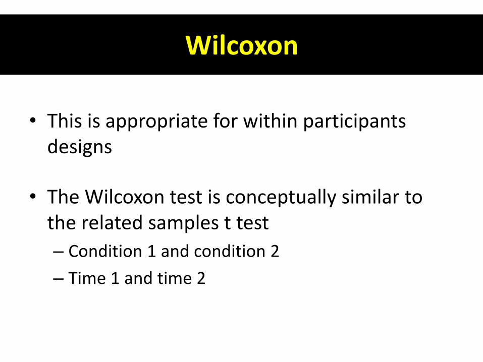
• This is appropriate for within participants designs
• The Wilcoxon test is conceptually similar to the related samples t test
– Condition 1 and condition 2
– Time 1 and time 2
Wilcoxon
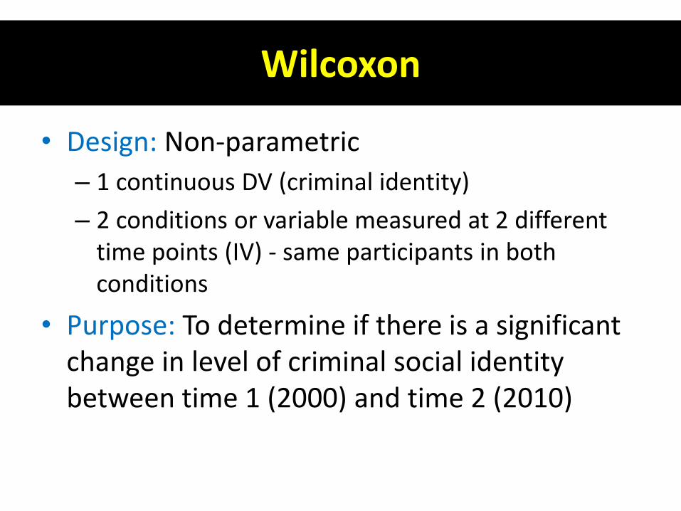
• Design: Non-parametric
– 1 continuous DV (criminal identity)
– 2 conditions or variable measured at 2 different time points (IV) - same participants in both conditions
• Purpose: To determine if there is a significant change in level of criminal social identity between time 1 (2000) and time 2 (2010)
SPSS Procedure
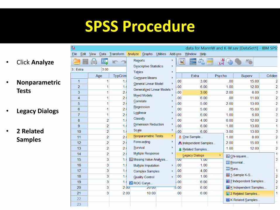
• Click Analyze
• Nonparametric Tests
• Legacy Dialogs
• 2 Related Samples
SPSS Procedure
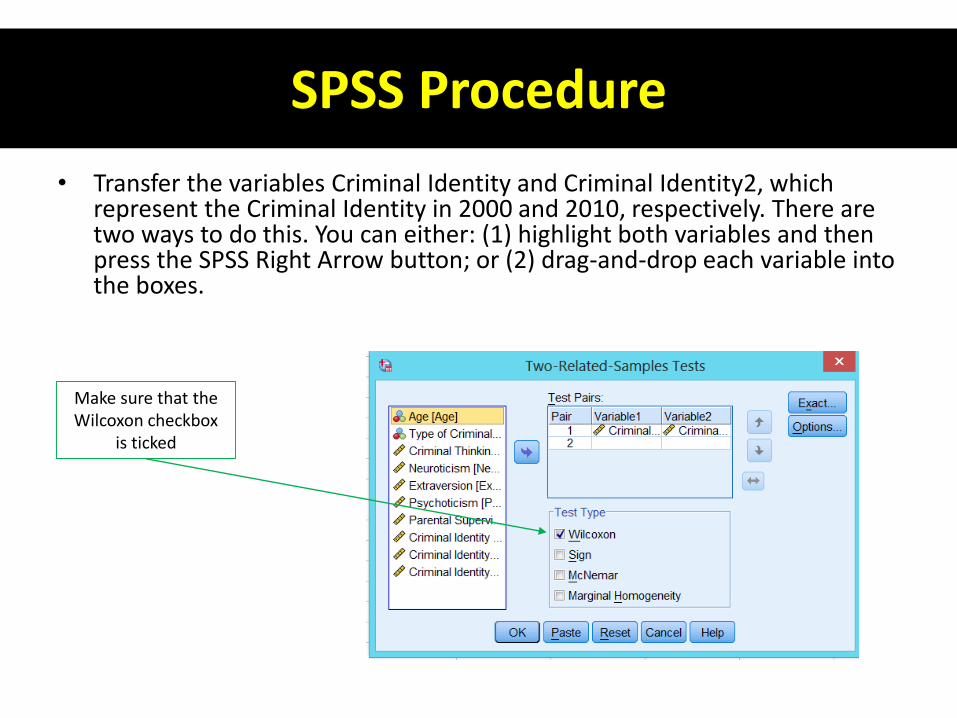
• Transfer the variables Criminal Identity and Criminal Identity2, which represent the Criminal Identity in 2000 and 2010, respectively. There are two ways to do this. You can either: (1) highlight both variables and then press the SPSS Right Arrow button; or (2) drag-and-drop each variable into the boxes.
Make sure that the Wilcoxon checkbox
is ticked
SPSS Procedure
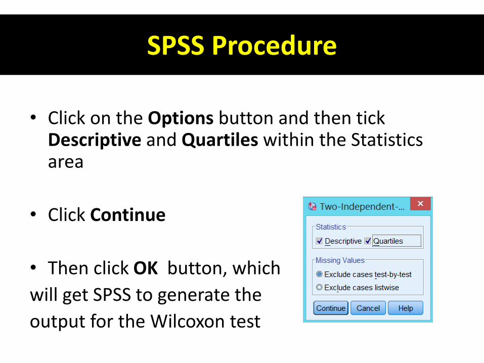
• Click on the Options button and then tick Descriptive and Quartiles within the Statistics area
• Click Continue
• Then click OK button, which
will get SPSS to generate the
output for the Wilcoxon test
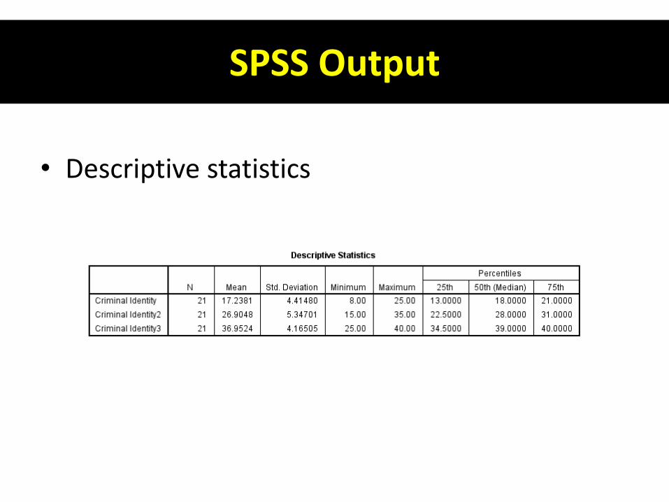
SPSS Output
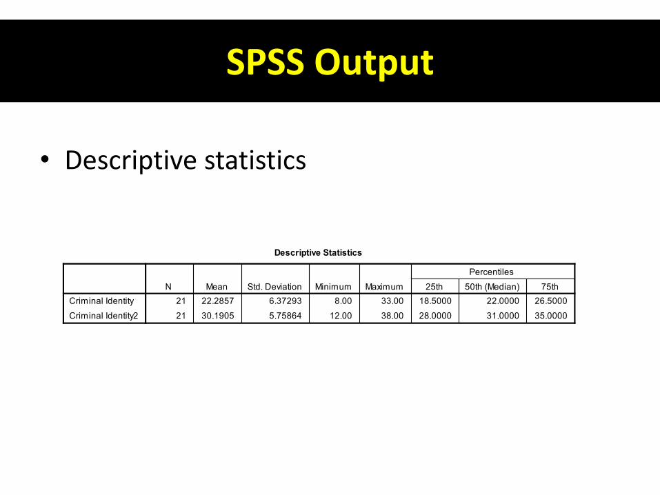
• Descriptive statistics

SPSS Output
• The Ranks table provides some interesting data on the comparison of prisoners' criminal identity sores at time 1 and time 2.
• We can see from the table's legend that none of the prisoners in 2000 had a higher scores than in 2010. All of them had a higher Criminal Identity Score in 2010 and none of them saw no change in their score
SPSS Output
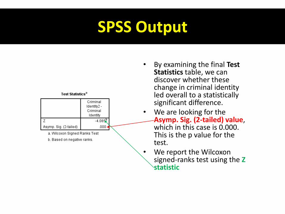
• By examining the final Test Statistics table, we can discover whether these change in criminal identity led overall to a statistically significant difference.
• We are looking for the Asymp. Sig. (2-tailed) value, which in this case is 0.000. This is the p value for the test.
• We report the Wilcoxon signed-ranks test using the Z statistic

Effect Size
• Must be calculated manually, using the following formula:
Z
𝑁
-4.085
√42
r = ̶ ̶̶ ̶ ̶̶
r = ̶ ̶̶ ̶ ̶̶
The N here is the total number of observations that were made (typically, participants x 2 when you have two levels) – this example r = - .63 (large effect size)
Reporting Wilcoxon
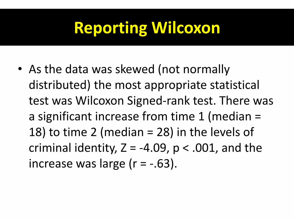
• As the data was skewed (not normally distributed) the most appropriate statistical test was Wilcoxon Signed-rank test. There was a significant increase from time 1 (median = 18) to time 2 (median = 28) in the levels of criminal identity, Z = -4.09, p < .001, and the increase was large (r = -.63).

Friedman’s test
• The Friedman’s test is the nonparametric test equivalent to the repeated measures ANOVA, and an extension of the Wilcoxon test
– it allows the comparison of more than two dependent groups (two or more conditions)
Friedman’s test
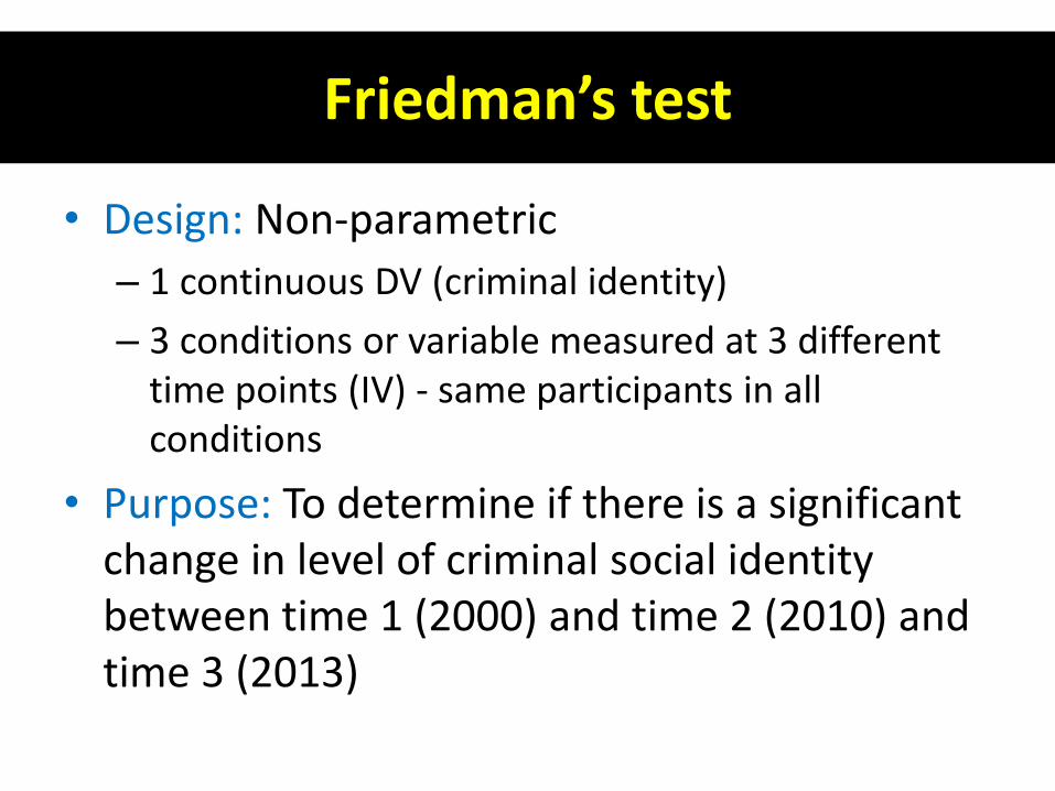
• Design: Non-parametric
– 1 continuous DV (criminal identity)
– 3 conditions or variable measured at 3 different time points (IV) - same participants in all conditions
• Purpose: To determine if there is a significant change in level of criminal social identity between time 1 (2000) and time 2 (2010) and time 3 (2013)

SPSS Procedure
• Click Analyze
• Nonparametric Tests
• Legacy Dialogs
• K Related Samples

SPSS Procedure
• Move all levels of DV (this example “Criminal Identity” “Criminal Identity1” “Criminal Identity2” to the Test Variable: box by using the SPSS Right Arrow button
Make sure that the Friedman checkbox
is ticked
SPSS Procedure
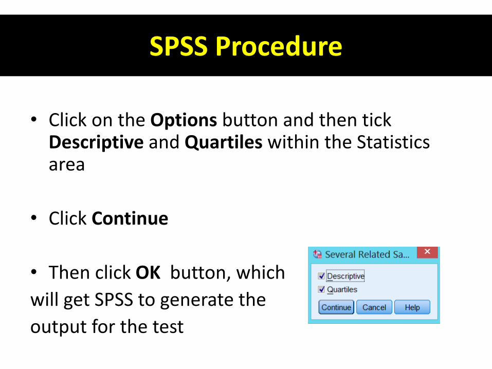
• Click on the Options button and then tick Descriptive and Quartiles within the Statistics area
• Click Continue
• Then click OK button, which
will get SPSS to generate the
output for the test
SPSS Output
• Descriptive statistics

SPSS Output
• There was a significant change in levels of criminal social identity over time, χ2(2, N = 21) = 42.00, p < .001.
χ2 value should be reported with degree of freedom
You should generally report the asymptotic p value

Following-up a Significant K-W Result
• If overall Friedman test is significant, conduct a series of Wilcoxon tests to identify where the specific differences lie, but with corrections to control for inflation of type I error.
• No option for this in SPSS, so manually conduct a Bonferroni correction ( = .05 / number of comparisons) and use the corrected -value to interpret the results– This example .05/3 = .016 – Reminder: Bonferroni corrections are overly
conservative, so they might not be significant.
Tip!
• If you have many levels of the IV (“repetitions,” “times,” etc.) consider comparing only some of them, chosen according to
– theory or your research question
– Or time 1 vs. time 2, time 2 vs. time 3, time 3 vs. time 4, etc.
Reporting Kruskal-Wallis
• In our example, we can report that there was a statistically significant increase in criminal social identity from year 2000 (median = 18) to 2010 (median = 28) and 2013 (median = 39) (χ2(2, N = 21) = 42.00, p < .001.
• Also report the post-hoc tests with effect size (see lecture on Wilcoxon test)