Embed Size (px)
Citation preview

Mon. Not. R. Astron. Soc. 315, 165±183 (2000)
Non-linear av-dynamos driven by magnetic buoyancy
J.-C. Thelenw²Department of Applied Mathematics, University of Leeds, Leeds LS2 9JT
Accepted 2000 January 17. Received 1999 October 4; in original form 1999 April 8
A B S T R A C T
It is now widely accepted that the large-scale solar magnetic field is generated by some kind
of non-linear av-dynamo. However, these dynamos have the disadvantage that the non-
linearities, and in particular the a -effect, are chosen in an ad hoc fashion and are only
vaguely related to the underlying physical processes.
Here, on the other hand, an av -dynamo with an a -effect based on magnetic buoyancy
instabilities is described. This a -effect has one main advantage over previous descriptions,
namely that it is derived from a numerical model of the physical processes that are thought
to occur at the base of the convection zone.
In this paper we investigate a one-dimensional and a two-dimensional av -dynamo in a
cylindrical and a spherical shell, respectively. In both models the v -effect is described by a
simple shear flow, while a is proportional to the radial gradient of the magnetic field
because, simply speaking, this gradient determines when magnetic buoyancy instabilities
occur and hence when the a -effect sets in.
Key words: instabilities ± MHD ± Sun: magnetic fields ± sunspots.
1 I N T R O D U C T I O N
Lower main sequence stars display a cyclic magnetic activity,
which is characteristic of stars with a deep convection zone. The
degree of magnetic activity depends on both the angular velocity
and the spectral type of the star and it is considered to be a
function of the inverse Rossby number s � Vtc; where V is the
angular velocity and tc is a suitable convective time-scale (Noyes,
Weiss & Vaughan 1984). The most active stars are young stars
with very short rotation rates of the order of a day or less. As the
star becomes older its rotation rate decreases owing to magnetic
braking, i.e. owing to the torque exerted by the stellar wind, and
the star becomes less active. The Sun, which concerns us here, at
4:5 � 109 yr; is a weakly active middle aged star with a magnetic
cycle which oscillates irregularly with a mean period of 22 yr,
taking into account the reversal of the polarity of the magnetic
field (Weiss 1993).
It is widely believed that the magnetic cycle is generated by
some type of hydrodynamic dynamo. The most common approach
to study such a dynamo is to make use of mean-field dynamo
theory. Here, the magnetic field is split into its mean and
fluctuating parts and an equation for the mean part is derived by
parametrizing the interaction between the small-scale magnetic
field and the turbulent velocity field. The most important
parameter is the a -effect which relates the mean electric
current to the mean magnetic field. In most mean-field dynamos
the a -effect is thought to be the result of helical motions resulting
from the interactions of the convective turbulence and rotation
(Parker 1955).
The first kinematic mean-field dynamo was developed by
Steenbeck & Krause (1969) and their simple model already agreed
with some of the solar observations such as the butterfly diagram
and Hale's polarity laws. Similar models were investigated by
Roberts (1972), Jepps (1975) and more recent kinematic models
include those by Schmitt (1987), Prautzsch (1993) and Parker
(1993).
However, all the above mentioned kinematic models have the
disadvantage that the growth of the magnetic field is unlimited. In
order to inhibit this unlimited growth, it is necessary to include
non-linear effects into the basic dynamo equations. Several field
limiting mechanisms have been proposed so far. First, a-quenching,
which is in essence an arbitrary non-linearity, based on the plausible
physical argument that a strong magnetic field exhibits a strong
resistance to deformations by small-scale motions. The arbitrari-
ness results from the fact that the exact physics of the solar
interior, such as the flux tubes and the form of convection, are not
known and that therefore it is necessary to rely on a parametriza-
tion. Dynamo models incorporating this type of non-linearity have
been investigated by Brandenburg et al. (1989a), Brandenburg,
Tuominene & Moss (1989b), Covas et al. (1997a,b), Jennings
(1991) and Jennings & Weiss (1991). Secondly, the effectiveness
of the v-effect can be reduced, either by v-quenching or by the
`Malkus±Proctor effect'. v-quenching, on the one hand, is an
arbitrary parametrization of the effect of the mean field on the
q 2000 RAS
w Current address: Department of Astronomy and Astrophysics, University
of Chicago, 5640 S. Ellis, Chicago, IL, 60637, USA.
² E-mail: [email protected]

differential rotation via either small scales or large scales
(Brandenburg et al. 1991; Jennings 1991; Jennings & Weiss
1991). The `Malkus±Proctor effect', on the other hand, does not
involve any parametrization and takes into account the effect of
the large-scale magnetic field on the driving velocity via the
Lorentz force (Malkus & Proctor 1975; Brandenburg et al. 1989a;
Schmitt & SchuÈssler 1989; Belvedere, Pitadella & Proctor 1990;
Tobias 1996, 1997). The final field limiting mechanism that has
been proposed is flux escape by magnetic buoyancy. This process
is based on the fact that the magnetic flux will eventually leave the
regions of field amplification owing to buoyancy and related
instabilities and hence will no longer contribute to the generation
of the magnetic field. (Schmitt & SchuÈssler 1989; Moss et al.
1990; Jennings 1991). An interesting model has been constructed
by Ferriz-Mas, Schmitt & SchuÈssler (1994) in which the dynamo
is driven by a non-axisymmetric instability of toroidal magnetic
flux tubes. The non-linear effect which finally limits the amplitude
of the dynamo results in a natural way from the mechanism which
drives the dynamo, namely the eruption of magnetic flux tubes
from the dynamo region.
An important question concerning these dynamo models is that
of their location. The assumption that the a -effect results from the
interaction of turbulent convection and rotation implies that the
dynamo is situated in the solar convection zone. However, there
are several problems associated with this idea. The most important
one concerns the difficulty of storing the magnetic flux in the
convection zone for periods comparable to the solar cycle.
Moreover, from self-consistent convection zone dynamos it emerges
that the toroidal magnetic field belts move toward the poles,
instead of towards the equator, for a surface differential rotation
which is consistent with that of the Sun (Gilman & Miller 1981;
Gilman 1983; Glatzmaier 1984, 1985). Therefore, for a variety of
reasons, based on results from magneto-convection (Spiegel &
Weiss 1980; Galloway & Weiss 1981), self-consistent dynamo
calculations of Gilman and Glatzmaier and helioseismology
(Brown et al. 1989), it is nowadays assumed that the dynamo is
located in the overshoot zone, a thin layer, situated between the
convection zone and the radiative zone. Locating the dynamo and
hence the magnetic field into the overshoot zone, nevertheless,
gives rise to another problem. As was mentioned before, dynamo
action in the convection zone relies on cyclonic motions, which
are caused by the interaction of convection and rotation. This
implies that in the overshoot zone the dynamo would be very
weak, or would even fail to operate, because of its subadiabatic
stratification. There are, however, several ways around this
problem. First, it is possible to split the dynamo into two parts,
with the v-effect and the a -effect confined to half space z , 0
and z . 0; representing the overshoot zone and the convection
zone, respectively. Such a dynamo has been investigated by Parker
(1993) in the kinematic regime and Tobias (1996, 1997) in the
non-linear regime. Secondly, convective motions are not neces-
sarily needed in order to obtain an a -effect. It has been shown by
Moffatt (1978), Schmitt (1985) and Thelen (1998, 2000) that a
mean-electromotive force, and hence an a -effect, can instead be
generated by helical waves resulting from magnetic buoyancy
instabilities. Schmitt (1987) and Prautzsch (1993) investigated
dynamo models in which the generation of the toroidal magnetic
field results from the induction effect of unstable magnetostrophic
waves. Their a-effect has the following latitudinal dependence: it
is negative near the equator and changes sign at mid-latitude to
become positive near the pole (Schmitt 1985). However, it was
shown by Thelen (1998, 2000) that this latitudinal dependence of
the a -effect is only valid in the case where the viscosity and the
magnetic diffusivity are neglected. If, on the other hand, viscous
effects are taken into account the latitudinal dependence can no
longer be determined, but some important insights into the radial
dependence of a can still be gained.
In this paper we therefore propose an av-dynamo that operates
in the overshoot zone with an a -effect based on magnetic
buoyancy instability. In particular, a is assumed to be proportional
to the radial gradient of the toroidal magnetic field since the
simplest criterion for magnetic buoyancy instabilities is that the
toroidal field strength decreases with height. In order to avoid any
unnecessary parametrizations the field growth is limited by the
`Malkus±Proctor' effect. Such a dynamo can operate in the over-
shoot zone without any difficulties since it does not depend on
turbulent convection. Moreover, this a has an advantage over
previous prescriptions in the sense that it is derived from a
numerical model of the physical processes which are thought to
occur in the overshoot zone. It should also be noted that the
cylindrical dynamo model has been chosen for simplicity since its
aim is not to obtain an accurate model but to show that magnetic
buoyancy instabilities are capable of a dynamo and to gain a basic
understanding of the underlying physical processes.
This paper is organized as follows. In Section 2 we describe
both the cylindrical and the spherical model, present the governing
equations and briefly explain the form of the a -effect. The results
for the cylindrical and the spherical dynamo models will be
presented in Sections 3 and 4, respectively. Finally in Section 5 a
conclusion is given.
2 M AT H E M AT I C A L F O R M U L AT I O N
2.1 The cylindrical shell model
Here, the overshoot zone is modelled by a cylindrical shell,
containing an electrically conducting and incompressible plasma,
with inner radius r0 and outer radius r1. Using mean-field dynamo
theory, the velocity field and the magnetic field are assumed to
have a small-scale structure. All quantities are assumed to be
axisymmetric, i.e. independent of f . Furthermore, the velocity is
assumed to be purely toroidal so that there is no meridional flow.
Initially, there is no toroidal magnetic field and the cylindrical
shell contains only a weak poloidal seed field. This poloidal seed
field is stretched into a field with a toroidal component by the
imposed differential rotation. This constitutes the v-effect which
is modelled by a simple, prescribed, radial shear flow, given by:
vpres�r� � Vpres�r�rf : �1�The a -effect which regenerates the poloidal field component from
a toroidal field component results from magnetic buoyancy
instabilities and is made to depend on the radial gradient of the
toroidal magnetic field strength. This is a reasonable assumption
since it has been shown that the interaction of magnetic buoyancy
instabilities and rotation gives rise to an a -effect (Moffatt 1978;
Schmitt 1985; Thelen 1998, 2000). Moreover, a simple criterion
for magnetic buoyancy instability is given by
2BT
r. 0 �2�
since, simply speaking, all that is required for magnetic buoyancy
instability to set in is a decrease with height of the magnetic field.
Furthermore, it was also shown that a is largest at the upper
interface between the magnetic layer and the non-magnetic layer,
166 J.-C. Thelen
q 2000 RAS, MNRAS 315, 165±183

i.e. in the region where the magnetic field falls off rapidly with
height. Hence, here a is assumed to be proportional to the
gradient of the toroidal magnetic field. Thus we choose to model
a (r, t) by
a�r� � 2a0
jBTjr
; ifjBTj
r, 0;
0; otherwise:
8<: �3�
From (3) it follows that initially a is zero since there is no toroidal
field and, assuming that the toroidal field BT is a smooth function
of r, a weak toroidal field corresponds to a weak a . This is
different from most av-dynamos where a (r) is always non-zero
and a is largest when the magnetic field is smallest.
The dynamical effect of the magnetic field is chosen to come
into play through the `Malkus±Proctor' effect, i.e. through its
effect on the f -component of the velocity (Malkus & Proctor
1975). The Lorentz force, which gives the back-reaction of the field
on the flow, induces a large-scale toroidal velocity vind subject to
viscous damping, in the opposite direction of the prescribed
azimuthal velocity. The total azimuthal velocity is then given by:
V tot � vpres � vind: �4�The Lorentz force and viscous damping are then the only terms to
appear in the f-component of the momentum equation. The
magnetic pressure and hence the gas pressure drop out owing to
axisymmetry and gravity only acts in the radial direction.
Similarly the inertial term vanishes because of axisymmetry and
because the flow is purely azimuthal.
This system is governed by the mean-field dynamo equations
BT
t� �72 2 r22�BT � r�BP ´ 7�V; �5�
A
t� �72 2 r22�A� DaBT �6�
and the momentum equation
vind
t� PM�72 2 r22�vind � �BP ´ 7�BT; �7�
where D � a0V00d3=h2 is the dynamo number and PM � nT=h is
the magnetic Prandtl number. Here BT and BP denote the toroidal
magnetic field and poloidal magnetic field, respectively. Equa-
tions (5)±(7) have been non-dimensionalized by introducing the
following variables:
r � r*d; t � t*d2
h; Bi � Bi*
d
h
����������m0r0
p; �8�
where d is the layer depth and d2/h is the magnetic diffusion time.
In order to reduce the system (5)±(7) to one dimension only one
Fourier mode is retained and the solutions A and BT are assumed
to be of the form:
A�r; z; t� � R�A�r; t� exp�ikz��; �9�BT�r; z; t� � R�B�r; t� exp�ikz��; �10�where Aà and Bà are complex. Note that for such a magnetic field
the Lorentz force, and therefore the induced velocity will not be
z-independent. In order to eliminate the z-dependence two
different approaches have been used. First, the induced velocity
is assumed to be independent of z, i.e. the Lorentz force has
been truncated at zeroth order in the z-direction. This is the
equivalent of only retaining the z-averaged component of the
Lorentz force. Thus after substituting (9) and (10) into (5)±(7),
and dropping `hats' for convenience, the following system of
partial differential equations is obtained:
B
t� �72 2 r22 2 k2�B 2 irk
V
rA; �11�
A
t� �72 2 r22 2 k2�A� DaB; �12�
vind
t� PM�72 2 r22�vind � ik
4
r�A*B 2 AB*�
� �� ik
2r�A*B 2 AB*�: �13�
Secondly, a higher order system is obtained by retaining the second-
order terms of the Lorentz force and by truncating the other non-
linear terms at the third order in z. This gives rise to an additional
equation for the induced velocity. Proceeding as above we obtain:
B
t� �72 2 r22 2 k2�B 2 irk
V
rA� irkv
A*
r
� ikvA*� irk
2
v
rA*; �14�
A
t� �72 2 r22 2 k2�A� DaB; �15�
vind
t� PM�72 2 r22�vind � ik
4
r�A*B 2 AB*�
� �� ik
2r�A*B 2 AB*� �16�
and
wind
t� PM�72 2 r22 2 4k2�wind � ik
2
A
rB 2
B
rA
� �: �17�
Here `*' denotes the complex conjugate, vind is real and wind is
complex. The two systems (11)±(13) and (14)±(17) will
subsequently be studied. Here V is again given by:
V � Vpres � vind=r; �18�while v is given by
v � wind=r; �19�where vind is the induced velocity resulting from the zeroth-order
terms in the Lorentz force and wind is the induced velocity
resulting from to the second-order terms. These two systems are
then solved subject to the following boundary conditions. First, it
is assumed that the base of the overshoot zone is a perfect
conductor. Hence the radial component of the magnetic field and
the tangential component of the electric field vanish there, i.e.
A � 0 andBr
r� 0 at r � r0: �20�
Secondly, the top boundary of the overshoot zone is assumed to be
perfectly insulating. Hence there are no currents in the region above
our layer which implies that the toroidal magnetic field has to
vanish and that the field matches a potential field at the surface, i.e.
B � 0 andA
r� cA � 0 at r � r1; �21�
where r1 � r0 � 1 since the layer depth has been chosen as
the unit of length. The boundary condition for the velocity has
been chosen to be stress-free at the top and slip-free at the
Non-linear av-dynamos driven by magnetic buoyancy 167
q 2000 RAS, MNRAS 315, 165±183

bottom, i.e.
V tot � 0 at r � r1 andV tot=r
r� 0 at r � r0: �22�
It is important to notice that equations (11)±(13) and (14)±(17)
have been obtained by averaging over latitude and retaining the
radial dependence. This is contrary to most one-dimensional
av-dynamo models which normally only keep the latitudinal
dependence (see for example Weiss, Catteneo & Jones 1984;
Jennings 1991). This approach results directly from our prescrip-
tion of the a -effect since a is driven by the radial gradient of the
toroidal magnetic field and therefore it has to be a function of
radius.
2.2 The spherical shell model
Here, the one-dimensional dynamo, described in the previous
section, is extended to a two-dimensional spherical shell model.
The two dynamo models are basically identical except for the
description of the a -effect. In the one-dimensional model it was
assumed that magnetic buoyancy, and hence the a -effect sets in as
soon as the magnetic field strength falls off with height (see
equation 3). This is strictly speaking not true since in general the
magnetic buoyancy instability must be vigorous enough to
overcome the stabilizing influence of the stratification of the
atmosphere and various other effects. Thus the radial gradient of
the magnetic field strength must exceed a certain threshold value
in order for magnetic buoyancy to occur. Therefore, in this model,
the a -effect will only set in if the following condition is satisfied:
jBTjr
, 2C; �23�
where BT is the toroidal field strength and C is assumed to be a
measure of the stabilizing effect of the atmospheric stratification.
This is based on the instability criterion for axisymmetric modes:
2g
gc2s
d
dzln
BT
r
� �.
N2
V2�24�
or for non-axisymmetric modes:
2g
gc2s
d
dz�ln�BT�� . k2
y 1� k2z
k2x
� �� N2
V2; �25�
where N is the Brunt±Vaiasala frequency (Acheson 1979).
Moreover, since the latitudinal dependence of a is not known,
we choose, for the sake of simplicity, a to be positive in the
northern hemisphere and negative in the southern hemisphere. It
should, however, be noted that results from helioseismology
suggest that in the neighbourhood of the equator a needs to be
negative at the base of the convection zone. Thus we choose to
model a (r, u , t) by:
a�r; u� � a�r� sin�2u�; 2 p=2 # u # p=2; �26�where
a�r� � 2a0BT
jBTjr
2 C; if BT
jBTjr
, 2C;
0; otherwise:
8<: �27�
Here, C, is added to the stability criterion in order to avoid a
spatial discontinuity which would otherwise occur. For physical
reasons, only positive values of C will be considered since these
correspond to a stably stratified atmosphere. Finally, C . 0
ensures that the a -effect vanishes for zero toroidal magnetic field.
In order to get an equatorward migration of the toroidal field belt
it is required that a (v /r) is negative in the northern hemisphere
and positive in the southern hemisphere. Moreover, the angular
velocity has to be symmetric about the equator and has to vanish
at the poles.
The governing equations of the two-dimensional spherical shell
dynamo are given by:
A
t� �72 2 r22 sin22 u�A� DBTa�r; u�; �28�
BT
t� �72 2 r22 sin22 u�BT � r sin uBP7
VT�r; u�fr sin u
� �; �29�
vind
t� PM�72 2 r22 sin22 u�vind � ��7 ^ B� ^ B�f: �30�
where D is the dynamo number and PM is the magnetic Prandtl
number. As in the previous section, equations (28)±(30) have been
non-dimensionalized using the layer depth d and the diffusion
time d2/h as units of length and time.
The above equations are then solved subject to the boundary
conditions (20), (21) and (22). Furthermore, the toroidal field B,
the vector potential A, the prescribed velocity vpres and the
induced velocity vind have to vanish at the poles. Thus:
A � BT � upres � vind � 0 at u � ^p=2: �31�
3 R E S U LT S F R O M C Y L I N D R I C A L S H E L L
DY N A M O
3.1 Zeroth-order truncation of the Lorentz force in Z
For the one-dimensional av-dynamo calculation performed here
a grid size of 51 grid points, uniformly spaced over r0 # r # r1
and a time-step of Dt � 1024 have been used. The inner radius has
been fixed at r0 � 2 while the magnetic Prandtl number was
chosen to be PM � 1: Changes in r0 and PM have no influence on
the qualitative behaviour of the system. Here it should also be
noted that equations (5)±(7) do not lend themselves to a linear
stability analysis since, as will be shown below, the initial
bifurcation point from the trivial steady state solution occurs at
infinity. This makes it impossible to determine the mode of maxi-
mum growth rate kmax and for this reason k has been arbitrarily
fixed at k � 1: This is one of the main disadvantages of this
model, although, changing the value of k, will most probably only
affect the amplitudes and the frequencies of the vector potential A
and the toroidal field, while their qualitative behaviour remains
unchanged.
The prescribed angular velocity is given by:
Vpres � 1:8 cos2�p�r 2 r0�=2�: �32�Taking the initial toroidal field to be B0 � 0 and the vector
potential A0 to be some seed field, finite amplitude solutions are
obtained for Ds $ 80: For these particular initial conditions lower
values of D do not yield dynamo action. However, note that the
dynamo number Ds at which non-trivial solutions occur depends
on the strength of the initial field. This is illustrated in Table 1,
which was obtained by keeping B0 � 0 fixed and varying the
strength of the initial poloidal seed field. Here we used
EA � 1
2
�1
0
jA0�r�j2 dr �33�
168 J.-C. Thelen
q 2000 RAS, MNRAS 315, 165±183

as a measure of the energy contained in the poloidal field. Thus as
the strength of the initial field is reduced Ds moves towards larger
values of D, while if the strength of the initial field is increased Ds
moves towards smaller values of D. The data in Table 1 suggests
that, as EA ! 0; the dynamo number Ds / E20:5A : Thus as EA
tends to zero Ds tends to infinity and the bifurcation from the
trivial solution to the finite amplitude solution is subcritical with
the bifurcation point at infinity. Furthermore, there seems to exist
a `critical' dynamo number Dc < 20 below which no dynamo
action occurs even for very strong magnetic fields. Here, it should
be noted that `critical' does not refer to the linear instability
threshold. Instead, by `critical' we mean that it is the lowest value
of the dynamo number D for which a non-trivial, stable solution
has been obtained. The simplest possible scenario that may give
rise to an oscillatory finite amplitude solution is that of a
subcritical Hopf bifurcation occurring at infinity with an unstable
branch extending back to Dc < 20; where a saddle-node bifur-
cation occurs as indicated in Fig. 1. This saddle-node bifurcation
is inherent to all three models discussed in this paper. Its existence
is a result of the fact that a finite value of D is required for dynamo
action. For D � 0 or for very small values of D the dynamo fails
to set in, independently of the initial field strength, because the
a -effect or the v-effect are not vigorous enough to maintain
dynamo action. The bifurcation at infinity, on the other hand,
results from the disappearanace of the a -effect in the absence of a
toroidal magnetic field. If the initial poloidal seed field is weak,
only a weak toroidal field will be generated by the differential
rotation, which translates into a small a . If D is large, this will be
enough to regenerate the poloidal field at a faster rate than the rate
at which it is destroyed by diffusion. If D is too weak the poloidal
field will decay and hence the dynamo will fail to set in. If,
however, the initial seed field is strong, then a strong toroidal field
and hence a large a is obtained and only a small D is required to
obtain dynamo action.
All the solutions obtained for the system of equations (11)±(13)
are periodic with a single frequency. Apart form the Hopf bifur-
cation at infinity and the saddle-node bifurcation at Dc, no other
bifurcations have been found. Furthermore, as D! 1 the induced
velocity tends to become uniform in space and time. Table 2
shows the amplitude of A, B and the frequency of the oscillations
for different values of the dynamo number D for PM � 1: As
D! 1 the following result is obtained:
jAj ! 1;jBj ! 0;
f ! const:
A similar result was obtained by Weiss et al. (1984) who
investigated a simple non-linear model of an oscillatory stellar
dynamo. They reduced the partial differential equations describing
the dynamo to a system of ordinary differential equations and
found that their simplest model, a fifth-order system, displayed a
similar behaviour to the one described above, while their higher
order systems were much more complicated.
Assuming that the induced velocity vind ! 2vpres; i.e. that the
shear becomes very small as D! 1; it is possible to show that:
A / D1=3; �34�B / D21=3: �35�Under the above assumption it is possible to eliminate the second
term on the right-hand side of equation (11) by putting:
V
r� Vpres
r� �vind=r�
r� 0 �36�
and hence:
vind � 2Vpresr � const: as D! 1: �37�Putting A � ~ADa and B � ~BDb and balancing the terms in
equations (11)±(13) it can easily be shown that (34) and (35) hold.
The constant of proportionality depends on the magnetic
Prandtl number and the layer depth. An increase in PM
corresponds to a decrease in the magnetic diffusivity and the
magnetic field behaves more and more as if it moved with the
plasma. Thus both the a and the v-effect become more effective
in generating the magnetic field, which lead to an increase in the
amplitude. This is shown in Fig. 2. Similarly the amplitudes of A
and B increased with decreasing layer depth. However, the exact
effect of varying the layer thickness could not be determined
because the value of the preferred latitudinal mode k, which most
likely changes with r0, is not known. In this case the value of k
becomes important since the chosen value of k may be more
favourable to dynamo action for thin layers than for thick layers.
Table 1. The dynamo number Ds at which non-trivial solutions occur as a function of the initialfield strength, for PM � 1 and r0 � 2:
EA 1/4 1/8 1/16 1/32 1/64 1/256
Ds 72 102 140 196 280 558
Figure 1. A possible bifurcation sequence that gives rise to periodic finite
amplitude solutions. A subcritical Hopf bifurcation occurs at D � 1: The
unstable branch (dashed line) extends back to Dc where a saddle-node
bifurcation occurs giving rise to a stable branch (continuous line) of finite
amplitude solutions.
Table 2. Amplitude of A, B and their frequencyfor PM � 1; r0 � 2 and for different values ofD.
D Amplitude Amplitude FrequencyA B
80 ^18.00 ^1.68 0.8100 ^21.36 ^1.64 0.7200 ^36.39 ^1.50 0.6400 ^56.88 ^1.33 0.6600 ^70.27 ^1.22 0.6800 ^79.97 ^1.13 0.6
1000 ^87.48 ^1.05 0.62000 ^110.6 ^0.84 0.64000 ^135.0 ^0.65 0.6
Non-linear av-dynamos driven by magnetic buoyancy 169
q 2000 RAS, MNRAS 315, 165±183

Thus the system (11)±(13) seems to be very robust. Changes in
the initial conditions, of the parameters D, PM and the layer depth
do not affect the overall behaviour of the system.
3.2 Second-order truncation of the Lorentz force in z
Here the influence of the dynamo number D on the behaviour of
the higher order system (14)±(17) will be studied. As it turns out
the behaviour of the solutions is much more complicated than for
the previous system, where only a simple periodic solution was
obtained. Here solutions with higher periods and chaotic solutions
occur and a much more elaborate bifurcation structure, including
features like hysteresis, has been obtained.
Fig. 3(a) shows the bifurcation diagram for 0 # D # 400; while
for larger values of D the behaviour is represented schematically
by Fig. 3(b). Fig. 3(a) is obtained by plotting EA, defined by
EA � 1
2�t1 2 t0��t1
t0
�1
0
jA�r; t�j2 dr dt �38�
against the dynamo number D. As in the previous section EA may
be considered to be a measure of the poloidal magnetic field
strength. [t0, t1] is the time interval over which the vector potential
has been averaged. Taking as initial condition B0 � 0 and A0 to be
some initial poloidal seed field, we obtain a periodic finite
amplitude solution for D $ 80: Note, however, that D � 80 is not
the critical dynamo number, because it was shown in the previous
section that the dynamo number at which the dynamo sets in
depends on the strength of the initial condition. The bifurcation
from the trivial state to the periodic solution is thus subcritical
with the bifurcation point at infinity. By taking the solution of
D � 80 as the initial condition and following the solution
backwards it turns out that it is possible to obtain dynamo action
for values of D as low as D < 20: Thus Dc < 20 is the `critical'
dynamo number since, as explained in Section 3.1, for D , Dc the
only stable solution which has been found is the trivial solution. If,
on the other hand, the dynamo is increased from D � 80 onwards,
the periodic solution persists up to D � 210: As the dynamo
number D is increased through D � 210 this lower branch
becomes unstable and an `upper' branch of periodic finite
amplitude solutions appears. This second solution distinguishes
itself from the previous one by having a larger frequency, a
smaller amplitude of the vector potential A and a larger amplitude
of the toroidal field B. This second solution is stable in the interval
165 # D # 260: As D is further increased beyond D � 260; this
solution becomes unstable and a period-five solution is obtained,
which persists in the interval 260 # D # 296: In order to gain a
better understanding of the behaviour of the system near D � 200
and D � 260 consider Fig. 4. This is a schematic representation of
the bifurcation diagram 3(a) in the interval 150 # D # 280: The
continuous lines represent the stable solutions obtained from our
numerical code, while the dashed lines show the simplest way in
which these stable branches might be connected by unstable
solutions. From this pictures it emerges that hysteresis is likely to
occur in the interval 165 # D # 210 and in the immediate vicinity
of D � 260:Finally, before chaotic solutions occur for D $ 302; a
Figure 2. (a) The amplitude of the vector potential as a function of D for
different values of r0. (b) The amplitude of the vector potential as a
function of D for different values of PM.
Figure 3. (a) Schematic representation of the bifurcation diagram up to
D � 310: Here stars represent periodic solutions and crosses chaotic ones.
(b) Occurrence of solutions at higher values of D. CH� chaotic, 1-P�period-one, 2-P� period-two.
Figure 4. Schematic representation of the bifurcation diagram 3(a). The
continuous lines indicate stable solutions found by our numerical code,
while the dashed lines represent possible unstable solutions.
170 J.-C. Thelen
q 2000 RAS, MNRAS 315, 165±183

period-seven solution is obtained in the short interval 299 #D # 302: The period-five and the period-seven solutions are
shown in Figs 5(a) and 6(a) for D � 270 and D � 300
respectively. In order to verify that the last two types of solutions
are indeed periodic and not quasiperiodic, their Poincare sections
and power spectra have been computed. The Poincare section is
obtained by projecting the trajectories of the solution in phase
space onto a suitable plane, in this case onto the (B, Vtot)-plane.
From the power spectrum it can clearly be seen that the
subharmonics are located at odd multiples of f1/5 and f1/7,
where f1 is the predominant frequency. This is shown in Figs 5(c)
and 6(c). Figs 5(b) and 6(b) show the corresponding PoincareÂ
sections. From Fig. 5(b) it is also apparent that the solution in
phase space intersects the (B, Vtot)-plane at five distinct points and
does not describe a closed curve which would be indicative of a
quasiperiodic solution. However, from the Poincare section for the
seven-periodic solution (see Fig. 6b) it is not that obvious anymore
that the phase-space solution intersects the (B, Vtot)-plane at seven
points. The spread of points in the Poincare section could be from
either numerical noise or the presence of a very long orbit, i.e.
very small frequency. Furthermore, since the value of D � 300 is
very close to the point where the seven periodic solution becomes
Figure 5. (a) B, A, Vtot of the period-five solution as a function of time at r � 2:4 for D � 270; PM � 1 and r0 � 2: (b) Poincare section of the period-five
solution. (c) Power spectrum of A.
Non-linear av-dynamos driven by magnetic buoyancy 171
q 2000 RAS, MNRAS 315, 165±183

unstable, the spread of points could also have been caused by a
very long initial transient. Chaotic solutions are obtained in the
range 302 # D # 4000: However, inside this interval 302 # D #4000 there exist several windows of periodicity. They are
enumerated below.
(i) Period-two solution in 610 # D # 780:(ii) Single periodic solution in 1160 # D # 1350:(iii) Period-two solution in 1680 # D # 2100:(iv) Single periodic solution in 2750 # D # 2800:
Thus, in this case, the route to chaos is the following: the trivial
solution gives rise to a periodic solution via a subcritical
bifurcation with the bifurcation point at infinity. A further
subcritical bifurcation gives rise to a second periodic solution
and chaos is then reached via a branch of period-five and a branch
of period-seven solutions. It should be noted no quasiperiodic
solutions have been obtained here.
A similar type of behaviour, namely the occurrence of jumps in
the energy levels, indicating the possibility of hysteresis (see Figs
3 and 4) and the existence of periodic solutions in the chaotic
interval, has also been observed by Covas et al. (1998). However,
they only obtained windows of periodicity in the case of thick
Figure 6. (a) B, A, Vtot of the period-seven solution as a function of time at r � 2:4 for D � 300; PM� 1 and r0 � 2: (b) Poincare section of the period-seven
solution. (c) Power spectrum of A.
172 J.-C. Thelen
q 2000 RAS, MNRAS 315, 165±183

shells, i.e. with an inner radius of r0 � 0:25; and that these
vanished for relatively thin shells with an inner radius of r0 � 2;such as have been considered in this section. Moreover, the
coexistence of two or three different stable solutions for the same
dynamo number depending on the initial conditions has also been
found by Belvedere et al. (1990) and Schmitt & SchuÈssler (1989).
This suggests that stars of a similar age and structure might
display different types of behaviour at any given time.
The system (11)±(13) and the system (14)±(17) have one char-
acteristic in common, namely that as D! 1; the amplitude of the
vector potential A goes to infinity, the amplitude of the toroidal
magnetic field B tends to zero and the amplitude of the induced
velocity vind, owing to the zeroth-order terms in the Lorentz force,
tends to some constant, i.e. it becomes steady. From this we may
conclude that the complicated behaviour of the system (14)±(17)
is because of wind, which is induced by the higher order terms
included in the Lorentz force.
3.3 The influence of the magnetic Prandtl number
Finally the consequences of changing the magnetic Prandtl
number on the different types of solutions will be considered.
Recent results from two-dimensional mean-field dynamos,
including the Malkus±Proctor effect, suggest that the dynamics
of the system depend on the magnetic Prandtl number. The period
of modulation of solutions, for example, seems to increase with
decreasing magnetic Prandtl number and grand minima only seem
to occur for PM ! 1: Physically this is because in order to obtain
grand minima the energy needs to be transferred between the
magnetic and the velocity field and there has to be a delay in the
quenching mechanism. In the case of the Malkus±Proctor effect
this delay corresponds to the time-scale on which the energy is
returned to the magnetic field, which is controlled by PM (Tobias
1996; Knobloch, Tobias & Weiss 1997). This might also explain
the absence of this type of modulated solution in our case, where
the magnetic Prandtl number PM is of order unity since the
exchange of energy between the magnetic field and the velocity
field occurs on too short a time-scale for the magnetic field to
decay by a considerable amount and thus the amplitude of the
oscillations remains constant. Furthermore, it was shown by Weiss
et al. (1984) and Jones, Weiss & Cattaneo (1985) that for low-
order models the bifurcation structure depended on the choice of
PM, with the periodic solutions remaining stable for PM . 1:In this investigation the following values of the magnetic
Prandtl number have been considered: PM � 2; PM � 0:5; PM �0:25: First, note that increasing PM leads to an increase in the
magnetic energy. This is, as expected, because for large PM the
magnetic field lines are stretched more rigorously and thus
stronger fields are obtained. However, the magnetic Prandtl
number seems to play an important part in the dynamics of our
model. For PM � 2 only periodic solutions have been obtained
which seems to confirm the above result that quasiperiodic
solutions only appear for PM , 1: Moreover, except for the short
interval of the period-three solution, the oscillatory solutions of
period one persist over long intervals of the dynamo number D.
This solution is still stable at D � 2000; at which stage the
computations have been stopped. At PM � 1 the solutions are still
periodic, but, as has been shown before, the overall behaviour is
less uniform and the bifurcation structure is more complicated.
The first quasiperiodic solution appears for PM � 0:5 in the short
interval 400 # D # 450 although the periodic solutions are still
predominant. However, PM � 0:5 is apparently still not small
enough to obtain `grand minima' type modulation. Thus in order
to check whether our model gives rise to such a behaviour some
calculations have been performed at lower values of PM. At PM �0:25 quasiperiodic solutions appear over a larger range of the
control parameter D. Furthermore the decrease of the magnetic
Prandtl number leads to the appearance of oscillatory solutions
with very large periods, which were absent in the case of PM � 2:For example, in the case of PM � 0:25 a period-nine solution was
obtained. No solutions have been obtained for lower values of the
magnetic Prandtl number, mainly because in order to ensure
convergence, a very large number of grid points is required, which
makes the investigation of the parameter space impractical. It
seems, however that `grand minima' type solutions, if they occur
in our model at all, will appear only for PM ! 1; which is in
agreement with Tobias (1996).
4 R E S U LT S F R O M S P H E R I C A L S H E L L
DY N A M O
4.1 PM . 1
The system of equations (28)±(30) is solved pseudospectrally by
expanding the vector potential A, the toroidal field B and the
induced velocity vind in Chebychev polynomials and associated
Legendre polynomials of order 1. By the term pseudospectral we
mean that the non-linear terms are evaluated in the physical space.
The time-stepping is performed by using a semi-implicit time-
integration scheme; the diffusion terms are calculated by a Crank±
Nicolson scheme in spectral space, while the non-linear terms are
calculated in physical space by using a two-step Adams±
Bashforth method. Both time-integration schemes are of second
order. The calculations have been performed by using either 32 �32 or 48 � 48 grid points, which is high enough a resolution in
order to ensure an exponential decay of high frequency modes. For
most of the calculations the inner radius is fixed at r0 � 2 and the
magnetic Prandtl number is given by PM � 3: For the same reason
as in Section 3, no linear stability analysis has been performed.
Taking B0 � 0 and A0 to be some seed field an oscillatory
dipole solution occurs at DD � 50; while an oscillatory quadru-
pole solution occurs at DQ � 70: It should, however, be noted that
the dynamo at which dynamo action occurs depends on the strength
of the initial field, i.e. as the initial field strength decreases DD and
DQ increase. Therefore, the bifurcation point from the trivial
steady state to a finite-amplitude solution is subcritical with the
bifurcation point at infinity. For a more detailed explanation see
Section 3. There also exists a critical dynamo number Dc below
which the dynamo fails to set in independently of the initial field
strength. In our calculation it actually turns out that DD (DQ) is
also the critical dynamo number for the oscillatory dipole
(quadrupole solution). This results from the relatively strong
initial poloidal field strength which was chosen here.
Next, the nature of the solution is investigated as the dynamo
number D is increased. First, stability tests have been performed in
order to see whether the pure dipole and the pure quadrupole
solutions are stable with respect to perturbations of the other
parity. In order to perform these calculations, EA, which is
considered to be a measure of the poloidal magnetic field strength,
is calculated according to:
EA � 1
2�t1 2 t0��t1
t0
�S
jA�r; u; t�j2 dS dt; �39�
where S is a meridional section of the spherical shell. Fig. 7 shows
Non-linear av-dynamos driven by magnetic buoyancy 173
q 2000 RAS, MNRAS 315, 165±183

the plot of EA versus the dynamo number D. Note that the energy
EA of both the dipole mode and the quadrupole mode seems to
level off as the dynamo number is increased. This is not too
surprising because it was shown previously that the amplitude of A
is proportional to D1/3 for large values of D.
However, the number of active regions in each hemisphere is
not exactly the same at any given time and hence it is reasonable
to assume that the solar magnetic field, which is responsible for
the appearance of sunspots, is slightly asymmetric about the
equator. Moreover, just as the Sun entered and emerged from the
Maunder minimum, sunspots were distributed asymmetrically
around the equator (Ribes & Nesme-Ribes 1993). Thus, since the
solar magnetic field seems to contain contributions from both
parities, the question arises as to what happens if the initial seed
field is of mixed parity. In order to study this case, the parity P of
the solution is considered. The parity is defined by:
P � ESA 2 EA
A
ESA � EA
A
; �40�
where ESA and EA
A denote the `energy' of the symmetric
(quadrupole) and antisymmetric (dipole) part of the vector poten-
tial in the conducting spherical shell (cf. Brandenburg et al.
1989a). ESA �EA
A � can easily be obtained from (39) by only
considering the coefficients with odd (even) n. Note that P � 1
corresponds to a pure quadrupole solution and that P � 21 to a
pure dipole solution. The stability of these mixed-mode solutions
is then investigated by adding an amount e of a quadrupole
component to a dipole and vice versa. Thus initially we have:
A0 � AA0 � eAS
0 �41�or
A0 � AS0 � eAA
0 : �42�Fig. 8 gives the evolution of the parity as a function of time for
D � 100; PM � 3; r0 � 2; C � 0 and different values of e . From
this it can clearly be seen that the final solution always has parity
P � 21; i.e. the final solution is always antisymmetric, except in
the case where the initial condition is a pure quadrupole. This also
holds at larger values of D. As the dynamo D is increased from Dc,
the dipole solution, represented by the continuous line in Fig. 7, is
found to be stable to quadrupole perturbations, while the quadru-
pole solution, represented by the dashed line, is unstable to dipole
perturbations. This, and the fact that they appear at slightly lower
values of D, suggests that, here, dipole solutions are preferred.
Furthermore, the evolution from the mixed-parity initial condition
to the pure dipole happens on a fairly short time-scale. The time
the solution takes to reach the dipole state is of order O(1),
independently of the initial value of the parity P, i.e. indepen-
dently of the relative strengths of the initial quadrupole and dipole
Figure 7. Plot of EA versus D for the dipole solution (A) and the
quadrupole solution (S) for PM � 3; r0 � 2 and C � 0: The continuous
line indicates that the dipole solution is stable to quadrupole perturbations,
while the dashed line indicates that the quadrupole solution is unstable to
dipole perturbations.
Figure 8. Evolution of the parity for D � 100; PM � 3; r0 � 2; C � 0 and different initial values of P.
174 J.-C. Thelen
q 2000 RAS, MNRAS 315, 165±183

components. A similar behaviour is observed for all values of
PM $ 1: In fact, changing PM does not alter the qualitative
behaviour of the system provided that PM $ 1 is satisfied, except
for an increase in the magnetic energy contained in the magnetic
field. This is because by increasing PM the magnetic diffusivity is
effectively reduced and hence the a -effect and the v-effect
become more effective in generating the magnetic field.
It should also be noted that all the solutions found in the large
magnetic Prandtl number regime are periodic in time, except for
two steady quadrupole solutions, which we will come to shortly.
The absence of quasiperiodic and chaotic solutions corresponds to
that found by Jones et al. (1985), who investigated the bifurcation
structure of a sixth order dynamo model and found that
quasiperiodic types of solutions only occur for PM , 1:Next the influence of the layer depth on the dynamo is
investigated. The following values for the inner radius r0 are
considered: r0 � 1 and r0 � 3: Higher values of r0 (thinner layers)
require a very high resolution and hence a large number of time-
steps in order to ensure stability and accuracy and are, therefore,
impractical to study. Increasing the inner radius r0 from r0 � 2 to
r0 � 3; i.e. decreasing the layer depth, leads to an increase in both
EA and EB and to a decrease in the critical dynamo number Dc.
Thus the dynamo becomes easier to excite, independently of the
initial conditions. In thick shells �r0 � 1� this situation is still valid
for the dipole solution, i.e. the energy contained in the magnetic
field is less than for either r0 � 2 or r0 � 3; and a larger D is
required for dynamo action. However, if the initial condition is
chosen to be a pure quadrupole then the situation changes
completely. First, instead of an oscillatory solution, a steady
solution is obtained and, secondly, this steady solution sets in at a
very low dynamo number compared to the corresponding dipole
solution. Unlike in all the previous cases, where the oscillatory
dipole was preferred over the oscillatory quadrupole, here the
steady quadrupole seems to be preferred over the oscillatory
dipole.
In order to investigate this behaviour the following initial
conditions are considered: B0 � 0 and A0 is chosen such that
EAA � ES
A �P � 0�; i.e. the initial energy contained in the dipole
component is the same as the initial energy contained in the
quadrupole component. Starting with this initial condition, a
steady quadrupole solution is obtained at D � 25; which is also
the critical dynamo number for the quadrupole solution. However,
for the same initial condition, a periodic dipole appears at D �350 and, following this solution backwards, the critical dynamo
number for the dipole solution is found to be D � 150: The graph
of EA versus the dynamo number D for both the dipole and the
quadrupole solution is shown in Fig. 9. For D , 350; the energy
contained in the quadrupole is larger than the energy contained in
the dipole, while for D $ 350 the reverse is true. Furthermore,
both the dipole and the quadrupole solutions are stable to
quadrupole and dipole perturbations, respectively. Thus, both
dipolar and quadrupolar solutions are possible stable solutions. A
similar behaviour was also observed by Brandenburg et al.
(1989a) in an investigation of an av-dynamo including the
Malkus±Proctor effect, except that in this case antisymmetric
solutions appeared at lower values of D than did symmetric
solutions. The final nature of the solution depends on the parity of
the initial condition, as can be seen from Fig. 10. From this graph
it emerges that at D � 225 the quadrupole solution is obtained for
20:2 # P # 1 and that the dipole solution is obtained for 21 #P 2 0:2: As D is increased further, dipole solutions are obtained
for values of P . 20:2: At D � 325 oscillatory dipole solutions
are obtained for P belonging to the interval 21 # P # 0:25 and
for D � 500 oscillatory dipole solutions occur for 21 # P #0:75:
Finally, returning to r0 � 2; the influence of the subadiabatic
stratification of the atmosphere, measured by the parameter C, is
considered. Here four different initial conditions are investigated,
namely
(i) a pure dipole poloidal seed field,
(ii) a mainly dipole poloidal seed field with a small quadrupole
component,
(iii) a pure quadrupole poloidal seed field,
(iv) a mainly quadrupole poloidal seed field with a small dipole
component.
First, for the pure dipole initial condition, increasing C,
(increasing the stabilizing effect of the atmospheric stratification)
does not result in a qualitative change in the nature of the periodic
solution. An increase in C just leads to a decrease in the magnetic
energy and moves the dynamo number at which dynamo action
occurs towards larger values of D. For large values of C, in this
case C . 1; it is difficult to obtain dynamo action even at large
values of D since the subadiabatic stratification suppresses the
a -effect very effectively. This is especially true for the initial
conditions with B0 � 0 since it then becomes nearly impossible to
obtain a steep enough gradient for dynamo action. A similar result
is obtained for a mainly dipolar initial condition. However, a pure
quadrupolar poloidal seed field results in a different behaviour.
For small values of C �C , 0:3� the solution is a periodic
quadrupole which behaves exactly as the dipole solution above.
As C is increased above C � 0:3; a steady quadrupole is obtained,
until at C � 1:5 the dynamo fails to set in. Finally, the behaviour
of the system for a mainly quadrupole poloidal seed field is shown
in Fig. 11. Here, the final solution, after the transients have died
away, is a pure dipole for 0 # C , 0:60: For larger values, how-
ever, the solution switches parity and becomes a steady quadru-
pole until for C . 1:5 the magnetic field starts to decay.
The investigation of the large Prandtl number regime gives rise
to two questions in particular. What are the physical reasons for
the appearance of the steady quadrupole mode and why is it, in
Figure 9. Plot of EA versus D for the dipole solution (A) and the
quadrupole solution (S) for PM � 3; r0 � 1 and C � 0: As opposed to
Fig. 7, both the dipole and quadrupole are stable to quadrupolar and
dipolar perturbations.
Non-linear av-dynamos driven by magnetic buoyancy 175
q 2000 RAS, MNRAS 315, 165±183
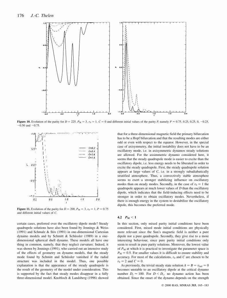
certain cases, preferred over the oscillatory dipole mode? Steady
quadrupole solutions have also been found by Jennings & Weiss
(1991) and Schmalz & Stix (1991) in one-dimensional Cartesian
dynamo models and by Schmitt & SchuÈssler (1989) in a one-
dimensional spherical shell dynamo. These models all have one
thing in common, namely, that they neglect curvature. Indeed, it
was shown by Jennings (1991), who carried out an intensive study
of the effects of geometry on dynamo models, that the steady
mode found by Schmitt and SchuÈssler vanished if the radial
structure was included in the model. Thus, one possible
explanation is that the appearance of the steady quadrupole is
the result of the geometry of the model under consideration. This
is supported by the fact that steady modes disappear in a fully
three-dimensional model. Knobloch & Landsberg (1996) showed
that for a three-dimensional magnetic field the primary bifurcation
has to be a Hopf bifurcation and that the resulting modes are either
odd or even with respect to the equator. However, in the special
case of axisymmetry, the initial instability does not have to be an
oscillatory mode, i.e. in axisymmetric dynamos steady solutions
are allowed. For the axsimmetric dynamo considered here, it
seems that the steady quadrupole mode is easier to excite than the
oscillatory dipole, i.e. less energy needs to be liberated in order to
excite the steady quadrupole. First, the steady quadrupole solution
appears at large values of C, i.e. in a strongly subadiabatically
stratified atmosphere. Thus, a convectively stable atmosphere
seems to exert a stronger stabilizing influence on oscillatory
modes than on steady modes. Secondly, in the case of r0 � 1 the
quadrupole appears at much lower values of D than the oscillatory
dipole, which indicates that the field-inducing effects need to be
stronger in order to obtain oscillatory modes. Nevertheless, if
there is enough energy in the system to destabilize the oscillatory
dipole, this becomes the preferred mode.
4.2 PM , 1
In this section, only mixed parity initial conditions have been
considered. First, mixed mode initial conditions are physically
more relevant since the Sun's magnetic field is neither a pure
dipole nor a pure quadrupole. Secondly, they give rise to a more
interesting behaviour, since pure parity initial conditions only
seem to result in pure parity solutions. Moreover, the lowest value
of PM at which it is practical to investigate the parameter space is
PM � 0:5: For smaller values it is difficult to ensure stability and
accuracy. For most of the calculations, r0 and C are chosen to be
r0 � 2 and C � 0:As previously, the trivial steady state solution A � B � vind � 0
becomes unstable to an oscillatory dipole at the critical dynamo
number Dc < 100: For D , Dc; no dynamo action has been
obtained. Since the onset of the dynamo depends on the strength
Figure 11. Evolution of the parity for D � 200; PM � 3; r0 � 1; P � 0:75
and different initial values of C.
Figure 10. Evolution of the parity for D � 225; PM � 3; r0 � 1; C � 0 and different initial values of the parity P, namely P < 0:75; 0.25, 0.25, 0, 20.25,
20.50 and 20.75.
176 J.-C. Thelen
q 2000 RAS, MNRAS 315, 165±183
of the initial condition, the bifurcation from the trivial steady state
to the dipole is subcritical with the bifurcation point at infinity.
This stable oscillatory dipole persists in the interval 100 # D #350: The time evolution of EA, EB, the kinetic energy EK and the
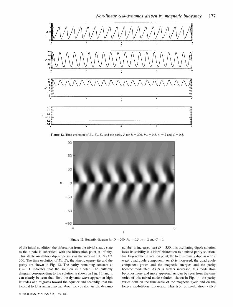
parity are shown in Fig. 12. The parity remaining constant at
P � 21 indicates that the solution is dipolar. The butterfly
diagram corresponding to the solution is shown in Fig. 13, and it
can clearly be seen that, first, the dynamo wave appears at high
latitudes and migrates toward the equator and secondly, that the
toroidal field is antisymmetric about the equator. As the dynamo
number is increased past D � 350; this oscillating dipole solution
loses its stability in a Hopf bifurcation to a mixed parity solution.
Just beyond the bifurcation point, the field is mainly dipolar with a
weak quadrupole component. As D is increased, the quadrupole
component grows and the magnetic energies and the parity
become modulated. As D is further increased, this modulation
becomes more and more apparent. As can be seen from the time
series of this mixed-mode solution, shown in Fig. 14, the parity
varies both on the time-scale of the magnetic cycle and on the
longer modulation time-scale. This type of modulation, called
Figure 12. Time evolution of EB, EA, EK and the parity P for D � 200; PM � 0:5; r0 � 2 and C � 0:5:
Figure 13. Butterfly diagram for D � 200; PM � 0:5; r0 � 2 and C � 0:
Non-linear av-dynamos driven by magnetic buoyancy 177
q 2000 RAS, MNRAS 315, 165±183

type I modulation, has been observed before by Moss et al. (1990),
Tobias (1997) and Covas (1998). At D < 625; this quasiperiodic
mixed mode solution loses its stability to a periodic mixed mode
solution. This type of solution remains stable in the interval 625 #D # 750: As can be seen from Fig. 16, which shows the time
evolution of the solution at D � 700; there is only one time-scale
present. As opposed to the previous quasiperiodic solution, the
parity is now solely oscillating with the frequency of the magnetic
cycle. However, in both these cases, the contribution of the
quadrupole component is much smaller than that of the dipole
component and hence the composition of the magnetic field is
mainly dipolar, except in the vicinity of the equator, where the
symmetry is broken, as can be seen from the butterfly diagram in Fig.
17. As a result of this there exists a small asymmetry between the
northern and the southern hemisphere. A similar mode was obtained
by Jennings (1991) and Jennings & Weiss (1991). They also obtained
a second type of periodic mixed mode solution, in which the
magnetic field is restricted to one hemisphere, while the other
hemisphere remains nearly free of magnetic activity. Such a mode
was not obtained here. As D is increased past D � 750; the periodic
Figure 14. Time evolution of EB, EA, EK and the parity P for D � 575; PM � 0:5; r0 � 2 and C � 0:
Figure 15. Butterfly diagram for D � 575; PM � 0:5; r0 � 2 and C � 0:
178 J.-C. Thelen
q 2000 RAS, MNRAS 315, 165±183

mixed mode solution loses stability, probably in a Hopf bifurcation,
and a second modulated mixed mode solution is obtained. From the
butterfly diagram in Fig. 19 it is clear that the asymmetry between
the northern and the southern hemisphere has become much more
pronounced. This modulated solution persists up to D � 1050;where, for numerical reasons, the calculations were stopped.
It should be noted that in this model no type II modulation has
been observed. Type II modulation is characterized by a change in
the amplitude which is not accompanied by a change in the parity.
The absence of this type of solution might result from the fact that
the calculations were stopped at D � 1050; but more likely the
reason is that the magnetic Prandtl number is not small enough. It
has been suggested by Tobias (1996, 1997) that the magnetic
Prandtl number controls the modulation of the frequency and that
the time-scale of the modulation varies as P0:5M : This implies that in
order for the ratio of the magnetic frequency to the modulation
frequency to be similar to that found on the Sun, i.e. so that the
minima occur roughly every 20 activity cycles, a value of PM �0:025 is required which is well beyond the limits of our numerical
scheme.
Figure 16. Time evolution of EB, EA, EK and the parity P for D � 700; PM � 0:5; r0 � 2 and C � 0:
Figure 17. Butterfly diagram for D � 700; PM � 0:5; r0 � 2 and C � 0:
Non-linear av-dynamos driven by magnetic buoyancy 179
q 2000 RAS, MNRAS 315, 165±183

In the low magnetic Prandtl number regime considered here, the
thickness of the spherical shell seems to play an important role in
the behaviour of the dynamo. In the case of a thick layer, i.e.
r0 � 1; none of the interesting solutions observed for r0 � 2
occurs, but the behaviour is identical to that described in the
previous section for r0 � 1 (see Fig. 9), except that EA and EB are
much smaller. For thin shells �r0 � 3�; on the other hand, the
behaviour of the system is similar to that described above. The
trivial steady state solution gives way to a periodic dipole solution
at the critical dynamo number Dc � 50; which persists in the
interval 50 # D # 100: As the dynamo number is increased past
D � 100; a modulated mixed mode solution is obtained, which
remains stable for values of D up to D � 300: Unfortunately, for
much larger values of D difficulties are encountered with respect
to numerical stability and accuracy and, therefore, the calculations
were stopped.
Finally, the consequence that changing C has on the nature of
the solution is investigated. Increasing C (making the atmosphere
more convectively stable) does not alter the bifurcation structure,
which has just been described, i.e. the periodic dipole solutions,
Figure 18. Time evolution of EB, EA, EK and the parity P for D � 1000; PM � 0:5; r0 � 2; and C � 0:
Figure 19. Butterfly diagram for D � 1000; PM � 0:5; r0 � 2; and C � 0:
180 J.-C. Thelen
q 2000 RAS, MNRAS 315, 165±183

the quasiperiodic mixed mode solutions and the periodic mixed
mode solution still appear in the same order. Even the bifurcation
points remain more or less at the same values of the dynamo
number D. The only difference which occurs is that the energy
contained in the magnetic field is reduced as C is increased.
However, it should be noted that only a small increase in C is
necessary in order to prohibit dynamo action. In this case, the
dynamo fails to set in for values of C < 0:1; compared to C < 1
in the large magnetic Prandtl number regime. This is probably
owing to the fact that for small PM the field inducing effects are
less effective and hence that the a -effect is more easily suppressed
by the subadiabatic stratification of the atmosphere.
Next we compare these solutions to the behaviour of the
magnetic field observed on the Sun. First, note that in this model
the dynamo waves appear at a relatively high latitude (<508)when compared to the butterfly diagrams obtained from observa-
tions, which indicate that sunspots appear between 30 and 40
degrees of latitude. Secondly, consider the butterfly diagram of the
periodic mixed mode solution, shown in Fig. 17. This solution is
nearly dipolar but there exists a slight north±south asymmetry
which is most obvious in the neighbourhood of the equator. As
similar asymmetry is actually observed on the Sun since the onset
of the solar cycles as well as the time of maximal sunspot intensity
are different in the southern and northern hemisphere. During the
normal solar cycle this asymmetry is very weak and therefore
Sokoloff & Nesme-Ribes (1994) suggested that there exists a
connection between this type of mixed parity solution and the
asymmetry in the solar cycle. Finally, let us turn to the two
quasiperiodic mixed mode solutions whose butterfly diagrams are
shown in Figs 15 and 19 and whose time evolution is shown in
Figs 14 and 18. They do not seem to correspond to either the
behaviour of solar magnetic fields during grand minima or that
displayed during normal solar activity. During the Maunder
minimum sunspots were mostly located in the southern hemi-
sphere between 0 and 220 degrees of latitude while very few
sunspots were observed in the northern hemisphere (Ribes &
Nesme-Ribes 1993; Sokoloff & Nesme-Ribes 1994). On the other
hand, during normal cycle activity the number of sunspots and
hence the magnetic field, varies nearly periodically with an
average period of 11 yr and does not seem to be modulated on a
longer time-scale. However, aysmmetric fields, which are distri-
buted over both hemispheres have also been observed. Observa-
tional data from the solar sunspot cycle in the Maunder minimum
(1645±1715) shows that when the magnetic field was weak, i.e.
just before and just after the Maunder minimum, both quadrupole
and dipole components were present and sunspots were distributed
asymmetrically (Ribes & Nesme-Ribes 1993). Numerical results,
mimicking this behaviour have recently been obtained by Beer,
Tobias & Weiss (1998).
5 C O N C L U S I O N
In the previous sections, we described an av-dynamo whose
a -effect is essentially the result of the interaction of magnetic
buoyancy instabilities and rotation. Our dynamo model contains
the three following non-linearities, namely the a -effect, the
v -effect and the Lorentz force. The a -effect is considered to be
proportional to the radial gradient of the magnetic field if the field
falls off with height and is chosen to be zero otherwise. The
Lorentz force allows us to take into account the back-reaction of
the magnetic field on the flow, which implies that the growth of
the magnetic field is limited by v-quenching.
The main consequence of the above a -effect is that the
bifurcation from the trivial state solution to a finite-amplitude
solution is subcritical and occurs at infinity. This result holds for
both the one-dimensional and the two-dimensional models
described here. The occurrence of the bifurcation point at infinity
is a consequence of the fact that for weak toroidal magnetic fields
the radial gradient of the field and hence a is small and that,
therefore, a large dynamo number D is required in order to obtain
dynamo action. Thus as the magnetic field strength tends to zero
the dynamo number D tends to infinity. This behaviour is in
contrast to that of many mean-field dynamo models investigated
so far, where the bifurcation from the trivial solution to the finite
amplitude solution occurs at a finite value of D. In these models ais either independent of the magnetic field strength or a is a
decreasing function of the magnetic field (Jepps 1975; Schmitt &
SchuÈssler 1989; Brandenburg 1989a; Covas 1998), as opposed to
the a chosen here which is an increasing function of the magnetic
field strength.
The fact that the initial bifurcation occurs at infinity is not very
likely in an astrophysical context. It would be more realistic to
have a subcritical (or supercritical) bifurcation at a finite value of
D. This could have been achieved by introducing an extra term
into the a -effect. The reason why it was decided not to do this was
to avoid introducing any unnecessary parameters into the
equations, whose physical meaning was not well understood.
The main results obtained from the cylindrical shell model are
the following. The first system, which is obtained by truncating
the Lorentz force at zeroth order is very robust with respect to
changes in the dynamo number D, the magnetic Prandtl number
PM and the layer depth. Only a single periodic finite amplitude
solution has been obtained, which remains stable for all values of
D and PM. Moreover, as the dynamo number tends to infinity, the
toroidal magnetic field strength goes to zero, the vector potential
and hence the poloidal field tends to infinity and the frequency
becomes constant. Moreover, the total velocity becomes uniform
in space and time as D is increased. This implies that the Lorentz
force drives a differential rotation which cancels out the
prescribed shear flow as D! 1: A similar result was obtained
by Weiss et al. (1984). The dynamics of the second system, on the
other hand, are far more complicated. First, a more complex
bifurcation structure is obtained. As opposed to the previous case,
where only one simple periodic solution was found, here solutions
with higher periods, such as period-five and period-seven
solutions, as well as chaotic solutions appear. Furthermore,
hysteresis occurred, i.e. in certain regions of parameter space
the solutions depend on the choice of the initial conditions. This is
interesting since it indicates that two stars of similar age and
structure might display two different types of behaviour. Secondly,
the behaviour of this system is no longer as robust as in the
previous case, in the sense that the bifurcation structure depends
now on the boundary conditions, the layer thickness and the
magnetic Prandtl number. The magnetic Prandtl number also plays
a very important role in the dynamics of the spherical shell
dynamo. For PM . 1 the solutions are in general periodic dipoles
or quadrupoles, while for PM , 1 quasiperiodic solutions appear.
This result corroborates that of Jones et al. (1985), namely that
periodic finite amplitude solutions only become unstable for
PM , 1: However, physically it is not clear why the behaviour of
the dynamo changes so abruptly at PM � 1: This question is
probably linked to the fact that in the large magnetic Prandtl
number regime only pure parity solutions seem to exist because
either the dipole or the quadrupole mode is damped if mixed
Non-linear av-dynamos driven by magnetic buoyancy 181
q 2000 RAS, MNRAS 315, 165±183

parity initial conditions are used. Thus type-I modulation,
characterized by a modulated parity, does not occur since it relies
on an exchange of energy between the dipole mode and the
quadrupole mode. Furthermore, type-II modulation, characterized
by either a constant quadrupole or dipole parity and a modulated
magnetic field, only arises at very low magnetic Prandtl numbers
and if the dynamo number D is sufficiently subcritical. This type
of modulation is based on an exchange of energy between the
magnetic field and the velocity field and can only occur if there is
a delay in the quenching mechanism. In our model this delay is
controlled by the magnetic Prandtl number and corresponds to the
time-scale on which the energy is returned to the field (Knobloch
et al. 1997). For small magnetic Prandtl numbers the behaviour of
the dynamo changes completely with the appearance of modulated
mixed mode solutions. However, type-II modulation, has not been
obtained, because the magnetic Prandtl number is not small
enough and the dynamo number is not sufficiently supercritical
enough. This is perhaps not too surprising since Tobias (1997)
showed that large values of PM shift type-II modulation to larger
values of D. Thus in order to obtain this type of modulation it is
necessary to decrease PM to values lower than those investigated
here. Decreasing PM, however, leads to difficulties since the
resolution and the number of time steps have to be increased in
order to ensure numerical stability. This problem is further
compounded by the fact that a decrease in PM reduces the
effectiveness of the field-inducing effects and that, therefore,
larger values of D are required in order to obtain dynamo action.
The results obtained here clearly indicate that it is possible to
drive an av -dynamo by an a-effect, which is based on magnetic
buoyancy instabilities. It should, however, be noted that the
behaviour of the solution is not in agreement with that observed in
solar type stars. By measuring the Ca+ emissions from active stars
it is possible to determine their rotation rates. It has been shown
that the most active stars are stars with short rotation periods and
moreover that their cycle frequency increases with the rotation
rate (see Weiss et al. 1984; Weiss 1993, and references therein).
Thus we would expect the toroidal magnetic field strength, which
can be considered to be a measure of the magnetic activity, to
increase with increasing D. However, in the system considered
here the toroidal magnetic field strength decreases. Furthermore,
modulation associated with changes in the parity have not been
observed in the Sun so far (Knobloch et al. 1997). Nevertheless,
some features of our results are consistent with solar observations.
First, the frequency of the oscillations increases with the dynamo
number. Secondly, in some regions of parameter space, our results
agree with observations of sunspots, which indicate that the solar
magnetic field is mainly dipolar and that it exhibits a small north±
south symmetry. Even though our results do not totally agree with
observations it is possible to conclude that such a dynamo may
well operate in the convectively stable overshoot zone or at the
base of the convection zone since the two key ingredients
necessary for dynamo action, namely the v-effect, resulting from
the strong radial gradient of the angular velocity, and the a -effect,
resulting from the interaction of magnetic buoyancy instabilities
and rotation, are present.
The main advantage of the dynamo model described in this
paper is that the a -effect is derived from a numerical model of the
physical processes operating in the overshoot zone. Therefore, this
a represents a physically more accurate model than the prescrip-
tions of the a -effect used in many models to date, which rely on
an ad hoc parametrization of the effects which are thought to
occur in the solar interior. Moreover, the growth of the magnetic
field is limited by taking account of the back-reaction of the field
on the flow through the Lorentz force and therefore it emerges
self-consistently from our model. Hence no extra parametrization
is needed. The main problem, on the other hand, is that, owing to
the prescription of the a -effect, it becomes impossible to
determine the latitudinal modes of maximum growth rate.
Furthermore, the latitudinal dependence of the a -effect is not
known and therefore it has been prescribed in such a way as to
give equatorward migration of the magnetic field. There are,
however, no physical reasons for this prescription. A further
disadvantage of these models is their inability to cope with very
low magnetic Prandtl numbers. This problem seems to be, at least
partially, inherent to the model under consideration. As PM tends
to zero the diffusive term, which balances the Lorentz force in
the momentum equation becomes negligible. Consequently, the
induced velocity grows rapidly until the direction of the flow is
reversed again by the Lorentz force. This growth of the induced
velocity results in a strong radial gradient of the azimuthal
velocity which is thought to lead to problems if the resolution is
too small.
AC K N OW L E D G M E N T S
I am grateful to David Hughes for all the helpful discussions. I am
indebted to Rainer Hollerbach for valuable help on spectral
methods and to an anonymous referee for some very helpful
comments on this paper. I would also like to thank PPARC for
paying my tuition fees.
R E F E R E N C E S
Acheson D. J., 1979, Phil. Trans. R. Soc. Lond., 289, 459
Beer J., Tobias S., Weiss N. O., 1998, Sol. Phys., 181, 237
Belvedere G., Pitadella R. M., Proctor M. R. E., 1990, GAFD, 51, 263
Brandenburg A., Krause F., Meinel R., Moss D., Tuominen I., 1989a,
A&A, 213, 411
Brandenburg A., Tuominene I., Moss D., 1989b, GAFD, 49, 129
Brandenburg A., Moss D., RuÈdiger G., Tuominen I., 1991, GAFD, 61, 179
Brown T. M., Christensen-Dalsgaard J., Dziembowski W. A., Goode P.,
Gough D. O., Morrow C. A., 1989, ApJ, 343, 526
Covas E., Tworkowski A. S., Brandenburg A., Tavakol R., 1997a, A&A,
317, 610
Covas E., Tworkowski A. S., Tavakol R., Brandenburg A., 1997b, Sol.
Phys., 172, 3
Covas E., Tavakol R., Tworkowski A. S., Brandenburg A., 1998, A&A,
329, 350
Ferriz-Mas A., Schmitt D., SchuÈssler M., 1994, A&A, 289, 949
Galloway D. J., Weiss N. O., 1981, ApJ, 243, 945
Gilman P. A., 1983, ApJS, 53, 243
Gilman P. A., Miller J., 1981, ApJS, 46, 211
Glatzmaier G. A., 1984, J. Comput. Phys., 55, 461
Glatzmaier G. A., 1985, ApJ, 291, 300
Jennings R. L., 1991, GAFD, 57, 147
Jennings R. L., Weiss N. O., 1991, MNRAS, 252, 249
Jepps S. A., 1975, JFM, 67, 625
Jones C. A., Weiss N. O., Cattaneo F., 1985, Phys. D, 14, 161
Knobloch E., Landsberg A. S., 1996, MNRAS, 278, 294
Knobloch E., Tobias S. M., Weiss N. O., 1997, MNRAS, 307, 1
Malkus W. V. R., Proctor M. R. E., 1975, JFM, 67, 417
Moffatt H. K., 1978, Magnetic Field Generation in Electrically Conducting
Fluids. Cambridge Univ. Press, Cambridge
Moss D., Tuominen I., Brandenburg A., 1990, A&A, 228, 284
Noyes R. W., Weiss N. O., Vaughan A. H., 1984, ApJ, 287, 769
Parker E. N., 1955, ApJ, 121, 293
182 J.-C. Thelen
q 2000 RAS, MNRAS 315, 165±183

Parker E. N., 1993, ApJ, 408, 707
Prautzsch T., 1993, in Proctor M. R. E., Matthews P. C., Rucklidge A. M.,
eds, Solar And Planetary Dynamos. Cambridge Univ. Press, Cambridge
Ribes J. C., Nesme-Ribes E., 1993, A&A, 276, 549
Roberts P. H., 1972, Phil. Trans. R. Soc. Lond. A, 272, 663
Schmalz S., Stix M., 1991, A&A, 245, 645
Schmitt D., 1985, PhD thesis, Univ. GoÈttingen
Schmitt D., 1987, A&A, 174, 281
Schmitt D., SchuÈssler M., 1989, A&A, 223, 343
Sokoloff D., Nesme-Ribes E., 1994, A&A, 228, 293
Spiegel E. A., Weiss N. O., 1981, Nat, 287, 616
Steenbeck M., Krause F., 1969, Astron. Nachr., 21, 1285
Thelen J.-C., 1998, PhD thesis, Univ. Leeds
Thelen J.-C., 2000, MNRAS, 315, 155 (this issue)
Tobias S. M., 1996, A&A, 207, L21
Tobias S. M., 1997, A&A, 322, 1007
Weiss N. O., 1993, in Proctor M. R. E., Gilbert A. D., eds, Lectures On
Solar and Planetary Dynamos. Cambridge Univ. Press, Cambridge
Weiss N. O., Cattaneo F., Jones C. A., 1984, GAFD, 30, 305
This paper has been typeset from a TEX/LATEX file prepared by the author.
Non-linear av-dynamos driven by magnetic buoyancy 183
q 2000 RAS, MNRAS 315, 165±183