NON-EQUILIBRIUM MOLECULAR DYNAMICS OF ELECTROMIGRATION

IN ALUMINUM AND ITS ALLOYS

FAT·IH GÜRÇA¼G SEN

SEPTEMBER 2006

NON-EQUILIBRIUM MOLECULAR DYNAMICS OF ELECTROMIGRATIONIN ALUMINUM AND ITS ALLOYS

A THESIS SUBMITTED TOTHE GRADUATE SCHOOL OF NATURAL AND APPLIED SCIENCES

OFMIDDLE EAST TECHNICAL UNIVERSITY

BY

FAT·IH GÜRÇA¼G SEN

IN PARTIAL FULFILLMENT OF THE REQUIREMENTSFOR

THE DEGREE OF MASTER OF SCIENCEIN

METALLURGICAL AND MATERIALS ENGINEERING

SEPTEMBER 2006

Approval of the Graduate School of Natural and Applied Sciences

Prof. Dr. Canan ÖZGEN

Director

I certify that this thesis satis�es all the requirements as a thesis for the degree of

Master of Science.

Prof. Dr. Tayfur ÖZTÜRK

Head of Department

This is to certify that we have read this thesis and that in our opinion it is fully

adequate, in scope and quality, as a thesis for the degree of Master of Science.

Assoc. Prof. Dr. M. Kadri AYDINOL

Supervisor

Examining Committee Members

Prof. Dr. Sakir BOR (METU, METE)

Assoc. Prof. Dr. M. Kadri AYDINOL (METU, METE)

Prof. Dr. ·Ishak KARAKAYA (METU, METE)

Assoc. Prof. Dr. Hakan GÜR (METU, METE)

Dr. Kaan PEHL·IVANO¼GLU (TÜB·ITAK, SAGE)

I hearby declare that all information in this document has been ob-

tained and presented in accordance with academic rules and ethical con-

duct. I also declare that, as required, I have fully cited and referenced all

material and results that are not original to this work.

Name Lastname : FAT·IH GÜRÇA¼G SEN

Signature :

iii

Abstract

NON-EQUILIBRIUM MOLECULAR DYNAMICS OF

ELECTROMIGRATION IN ALUMINUM AND ITS ALLOYS

SEN, FAT·IH GÜRÇA¼G

M.Sc., Department of Metallurgical & Materials Engineering

Supervisor: Assoc. Prof. Dr. Mehmet Kadri AYDINOL

September 2006, 99 pages

With constant miniaturization of integrated circuits, the current densities experi-

enced in interconnects in electronic circuits has been multiplied. Aluminum, which

is widely used as an interconnect material, has fast di¤usion kinetics under low tem-

peratures. Unfortunately, the combination of high current density and fast di¤usion

at low temperatures causes the circuit to fail by electromigration (EM), which is the

mass transport of atoms due to the momentum transfer between conducting electrons

and di¤using atoms. In the present study, the e¤ect of alloying elements in aluminum

on the di¤usion behaviour is investigated using a non equilibrium molecular dynamics

method (NEMD) under the e¤ect of electromigration wind force. The electromigra-

tion force was computed by the use of a pseudopotential method in which the force

depends on the imperfections on the lattice. 1.125 at% of various elements, namely

Cu, Mg, Mn, Sn and Ti were added into aluminum. The electromigration force was

then calculated on the alloying elements and the surrounding aluminum atoms and

these forces incorporated into molecular dynamics using the non-equilibrium formal-

ism. The jump frequencies of aluminum in these systems were then computed. Cu,

Mn and Sn impurities were found to be very e¤ective in lowering the kinetics of the

iv

di¤usion under electromigration conditions. Cu was known experimentally to have

such an e¤ect on aluminum for several years, but the Mn and Sn elements are shown

here for the �rst time that they can have a similar e¤ect.

Keywords: Electromigration, Di¤usion, Non-Equilibrium Molecular Dynamics, Alu-

minum Interconnect.

v

Öz

ALÜM·INYUM VE ALASIMLARINDA ELEKTROGÖÇÜN

MOLEKÜLER D·INAM·IK S·IMÜLASYONU

SEN, FAT·IH GÜRÇA¼G

Y. Lisans, Metalurji ve Malzeme Mühendisli¼gi Bölümü

Tez Yöneticisi: Doç. Dr. M. Kadri AYDINOL

Eylül 2006, 99 sayfa

Entegre devrelerin sürekli küçülmesiyle elektronik devre ba¼glant¬elemanlar¬nda olusan

ak¬m yo¼gunlu¼gu katlanarak artmaktad¬r. Bu tür devrelerde genis ölçüde kullan¬lan

Alüminyum metali, düsük s¬cakl¬kta h¬zl¬yay¬n¬m devinimine sahiptir. Ayn¬anda

hem yüksek ak¬m yo¼gunlu¼gu, hem de h¬zl¬yay¬n¬m devinimi, devrelerin elektrogöç

nedeniyle h¬zl¬bir sekilde bozulmas¬na neden olmaktad¬r. Elektrogöç, ak¬m içinde

ilerleyen elektronlar¬n momentumlar¬n¬atomlara aktarmalar¬yla olusan kütle hareke-

tidir. Bu çal¬smada, alüminyuma eklenen alas¬m elementlerinin yay¬n¬m davran¬s¬na

etkisi, elektrogöç kuvveti alt¬nda, denge d¬s¬moleküler dinamik yöntemiyle incelen-

mistir. Elektrogöç kuvveti, kuvvetin kafes içindeki hatalara ba¼gl¬oldu¼gu psödopotan-

siyel metodu ile hesaplanm¬st¬r. Çal¬smada, Cu, Mg, Mn, Sn ve Ti elementleri,

%1,125 atom oran¬nda alüminyuma eklenmistir. Elektrogöç kuvveti, eklenen alas¬m

elementleri ve bu elementleri çevreleyen alüminyum atomlar¬üzerinde hesaplanarak

denge d¬s¬ durumu ile moleküler dinamik yöntemine dahil edilmistir. Daha sonra

alüminyum atomlar¬n¬n atlama frekans¬hesap edilmistir. Elektrogöç kosullar¬alt¬nda

yay¬n¬m devinimi azaltmada Cu, Mn ve Sn katk¬lar¬n¬n çok etkili oldu¼gu görülmüstür.

Bak¬r¬n, alüminyum içinde böylesi bir etkiye sebep oldu¼gu deneysel çal¬smalar sonu-

vi

cunda uzun zamand¬r bilinmektedir ancak Mn ve Sn elementlerinin de buna benzer

etkileri oldu¼gu ilk defa gösterilmistir.

Anahtar Kelimeler: Elektrogöç, Yay¬n¬m, Moleküler Dinamik, Alüminyum ba¼glant¬

eleman¬

vii

To my family

viii

Acknowledgements

I would like to express my sincere gratitude to my supervisor Kadri Ayd¬nol for his

valuable guidance and support during the study of this thesis. I also thank to him

for his endless patience to me.

I deeply thank my friends, Tufan Güngören and Alper K¬nac¬for their valuable sug-

gestions and support during the period of this study.

I specially thank to my friends Evren Tan, Güher Kotan, Melih Topçuo¼glu, Bar¬s

Okatan, Hasan Aky¬ld¬z, Betül Akköprü, Ziya Esen, Ali Erdem Eken, Doruk Do¼gu,

Caner Simsir, Kemal Davut, Gül Çevik, Selen Gürbüz for their valuable support

during the period of writing this thesis.

I am grateful to my family, Azize, Sadi and Ayça Sen for their encouragement and

constant support during the period of this study.

The numerical calculations reported in this study were carried out at the ULAK-

BIM High Performance Computing Center at the Turkish Scienti�c and Technical

Research Council (TUBITAK). I specially thank to the member of this facility Onur

Temizsoylu for his constant help during the usage of this super computing facility.

ix

Table of Contents

plagiarism . . . . . . . . . . . . . . . . . . . . . . . . . . . . . . . . . . . . . . . . . . . . . . . . . . . . . . . . . . . . . iii

Abstract . . . . . . . . . . . . . . . . . . . . . . . . . . . . . . . . . . . . . . . . . . . . . . . . . . . . . . . . . . . . . . iv

Öz . . . . . . . . . . . . . . . . . . . . . . . . . . . . . . . . . . . . . . . . . . . . . . . . . . . . . . . . . . . . . . . . . . . . . . vi

Acknowledgements . . . . . . . . . . . . . . . . . . . . . . . . . . . . . . . . . . . . . . . . . . . . . . . . . . ix

Table of Contents . . . . . . . . . . . . . . . . . . . . . . . . . . . . . . . . . . . . . . . . . . . . . . . . . . . x

CHAPTER

1 Introduction . . . . . . . . . . . . . . . . . . . . . . . . . . . . . . . . . . . . . . . . . . . . . . . . . . . . . . 1

2 Molecular Dynamics . . . . . . . . . . . . . . . . . . . . . . . . . . . . . . . . . . . . . . . . . . . . . 4

2.1 Classical Molecular Dynamics . . . . . . . . . . . . . . . . . . . . . . . 4

2.1.1 History of Molecular Dynamics . . . . . . . . . . . . . . . . . . 4

2.1.2 Basics of Molecular Dynamics . . . . . . . . . . . . . . . . . . . 5

2.1.3 Property Calculations in Molecular Dynamics . . . . . . . . . . 21

2.2 Non-Equilibrium Molecular Dynamics . . . . . . . . . . . . . . . . . . 25

3 Potentials . . . . . . . . . . . . . . . . . . . . . . . . . . . . . . . . . . . . . . . . . . . . . . . . . . . . . . . . . 28

3.1 Pseudopotential theory . . . . . . . . . . . . . . . . . . . . . . . . . . 28

3.1.1 Model Potentials . . . . . . . . . . . . . . . . . . . . . . . . . . 29

3.1.2 Screening of the Pseudopotential . . . . . . . . . . . . . . . . . 34

x

3.2 Pair Potentials Derived by Pseudopotential Theory . . . . . . . . . . . 38

4 Pseudopotential based Electromigration theory . . . . . . . . . . . 42

4.1 Introduction . . . . . . . . . . . . . . . . . . . . . . . . . . . . . . . . . 42

4.2 Pseudopotential Based Electromigration Driving Force . . . . . . . . . 43

5 Methodology . . . . . . . . . . . . . . . . . . . . . . . . . . . . . . . . . . . . . . . . . . . . . . . . . . . . . 46

6 Results and Discussion . . . . . . . . . . . . . . . . . . . . . . . . . . . . . . . . . . . . . . . . . . . 56

6.1 Critical Potential Evaluation for Aluminum . . . . . . . . . . . . . . . 56

6.2 Electromigration Force Calculation Results . . . . . . . . . . . . . . . 59

6.3 Non-Equilibrium Molecular Dynamics Results . . . . . . . . . . . . . . 61

7 Conclusion . . . . . . . . . . . . . . . . . . . . . . . . . . . . . . . . . . . . . . . . . . . . . . . . . . . . . . . . . 69

References . . . . . . . . . . . . . . . . . . . . . . . . . . . . . . . . . . . . . . . . . . . . . . . . . . . . . . . . . . . . 70

APPENDICES

A List of Computer Program . . . . . . . . . . . . . . . . . . . . . . . . . . . . . . . . . . . . . 77

xi

Chapter 1

Introduction

Computer simulations play a very important role in materials science today. Com-

putational materials science acts as a bridge between experimental and theoretical

approaches. Computer simulations are often used both to solve theoretical models

beyond certain approximations and to provide a hint to experimentalists for further

investigations. Understanding the properties of materials in terms of their structure

and the microscopic interactions between them can be established by them. This

serves as a complement to conventional experiments. In addition to that, simulations

can be utilized not only to understand and interpret the experiments, but also to

study regions which are not accessible experimentally, or which would imply very

expensive experiments. Investigation of material properties and materials design by

using computers is cost e¤ective, in which the cost of characterization, synthesis,

processing and testing of materials are eliminated with the use of computer experi-

ments.

The traditional simulation methods for many-body systems can be divided into

two classes of stochastic and deterministic simulations, which are largely covered

by the Monte Carlo (MC) method [1] and the molecular dynamics (MD) method

[2, 3, 4], respectively. In addition to that there is a whole range of hybrid techniques

which combine features from both. Monte Carlo simulations probe the con�guration

space by trial moves of particles. Within the so-called Metropolis [1] algorithm, the

energy change between the following steps is used as a trigger to accept or reject the

new con�guration. Paths towards lower energy are always accepted, those to higher

energy are accepted with a probability governed by Boltzmann statistics. In that way,

properties of the system can be calculated by averaging over all Monte Carlo moves

(where one move means that every degree of freedom is probed once on average) [5].

1

By contrast, in MD methods; Newton�s equations of motion are integrated to

move particles to new positions and to get new velocities at these new positions. The

state of a dynamic system is given by its phase space coordinates at a certain time.

In MD, a dynamic system moves and changes its phase space coordinates in time,

evolving towards an internal equilibrium state of the whole system. The macroscopic

observables of the system are then obtained by suitably de�ned averages over the

phase space trajectory, at the internal equilibrium state of the whole system [6].

Molecular dynamics simulations allow us to calculate static properties as well as

dynamic properties of the system including transport properties.

Transport properties in materials are important as they describe how a material

relaxes back to equilibrium, following application of a mechanical or thermal pertur-

bation [7] . Introducing such perturbations into the equations of motion, produce

a time-dependent non-equilibrium distribution. At this point non-equilibrium mole-

cular dynamics (NEMD) method arises, which is �rstly announced by Hoover and

Ashurst [8]. NEMD methods are used to calculate transport properties such as vis-

cosity, self- and mutual di¤usion coe¢ cients, and thermal conductivity more precisely

than equilibrium methods [9].

Electromigration is the mass transport of a metal due to the momentum trans-

fer between conducting electrons and di¤using metal atoms. Electromigration has

been known for 100 years, but it is concerned with the development of the integrated

circuits. The thin �lms used as interconnects in integrated circuits have a thickness

in the order of 300 nm. Although a relatively small voltage (3.5-3.6 V) passes from

these interconnects, because of the small length over the applied voltage, very high

electric �eld was developed and consequently because of the small cross-section, very

high current density (106A/cm2) resulted due to Ohm�s Law. Furthermore, the con-

ductors were made of pure aluminum, a material with a low melting temperature,

which implies fast di¤usion at low temperatures. Such very thin �lm contains small

grains and thus many grain boundaries that are suitable for rapid di¤usion. This

combination of high current density and fast di¤usion at low temperatures causes

the circuit to fail due to vacancy di¤usion induced void formation and growth espe-

cially at grain boundaries. Intensive research has been carried out to overcome this

failure, for example, by adding few percentages of alloying elements like copper [10].

The electromigration was investigated theoretically in atomistic and phenomeno-

logical point of view in the literature. In the last decade several computer simulations

of electromigration in metal lines have been reported from the macroscopic point of

2

view [11, 12, 13]. However, as circuit integration shrinks to smaller dimensions, in-

�uences of crystal orientation and grain boundary structure on the lifetime must be

taken into account.

From the physics point of view, Sorbello [14, 15, 16] has made a very comprehen-

sive study about determining the driving force for electromigration for each individual

atom in a lattice. Sorbello has studied the atomic con�guration-dependent electro-

migration force including impurities and vacancies.

There are very limited studies in the literature involving atomistic simulations.

Molecular dynamics study of electromigration has been carried out by Ohkubo et al

[17]. In that study H type periodic boundaries for interconnects has been constructed

and 2 dimensional molecular dynamics simulations were carried out for aluminum.

In that study, the electromigration driving force was calculated using Cloud in Cell

(CIC) method and the evolution of the void formation was reported. Shinzawa and

Ohta [18] characterized the grain boundary di¤usion for aluminum interconnects by

molecular dynamics. The di¤usion characteristics with respect to the grain boundary

angle was reported. Maroudas and Gungor [19] studied the void evolution and failure

in metallic thin �lms. In that study, plastic deformations in the vicinity of the voids

are examined by the use of molecular dynamics.

In the development of an alloy with improved resistance to electromigration, we

should somehow eliminate grain boundaries or slow down the di¤usion process. Be-

cause of the stages in the processing of these interconnects, it is inevitable to have

grain boundaries. However it is possible to alter the di¤usion behavior with the

addition of alloying elements. Then the answer to the following question should be

given: Which alloying element would be e¤ective in lowering the di¤usion kinetics.

In the present study, therefore the e¤ect of alloying elements in aluminum to the bulk

di¤usion behavior is investigated using molecular dynamics method, under the e¤ect

of electromigration wind force.

Initially the MD method was reviewed in Chapter 2. The construction of a MD

simulation is explained in detail, including how a MD simulation can be started, how

the atomic interactions are handled, the integration methods used and how the prop-

erties of a material can be determined with the given algorithms. In Chapter 3, the

derivation of potentials is reported by introducing the pseudopotential method, and

how a pair potential can be obtained using this method. In Chapter 4, the pseudopo-

tential approach to the electromigration due to Sorbello was given. In Chapter 5, the

methodology followed is reported and the results obtained were given in Chapter 6.

3

Chapter 2

Molecular Dynamics

2.1 Classical Molecular Dynamics

2.1.1 History of Molecular Dynamics

The foundations of the Molecular Dynamics (MD) method has been laid by the de-

velopment of Newtonian dynamics by Isaac Newton. He proposed that the same

mechanical laws can explain the motions of all bodies, large and small, with suitable

de�nitions of the forces operative. Thus the Newtonian laws applies to systems of

any size, even to atoms. This concept has been modi�ed by quantum mechanics.

Then in classical statistical mechanics, Ludwig Boltzmann investigated the problem

of correlating the detailed dynamic behavior of a system of atoms and molecules with

the macroscopic experimentally measurable properties of the same system. These two

scienti�c approaches of classical dynamics and classical statistical mechanics consti-

tute the basis of the MD method. The trajectories and velocities of the particles

corresponding to atoms (or molecules, or ions) are generated using Newtonian equa-

tions of motion. Classical statistical mechanical concepts are then used to obtain the

correspondence of this system to a thermodynamic system.

The problem of studying the interaction of many atoms or molecules has only

become possible, using the methods of MD and MC, with the development of powerful

electronic computers after 1950�s.

The �rst papers reporting a molecular dynamics simulation were written by Alder

and Wainwright in 1957 [2, 3]. The purpose of the paper was to investigate the phase

diagram of a hard sphere system, and in particular the solid and liquid regions. In a

hard sphere system, particles interact via instantaneous collisions, and travel as free

4

particles between collisions.

Probably the �rst example of a molecular dynamics calculation with a continuous

potential based on a �nite di¤erence time integration method was done by Gibson

et al [20]. In that study, the calculation for a 500-atoms system was performed on

an IBM 704, and took about a minute per time step. A successful attempt to solve

the equations of motion for a set of Lennard-Jones particles was made by Rahman

[4]. Since that time the properties of the Lennard-Jones model have been thoroughly

investigated by Verlet [21, 22] in which Verlet time integration algorithm was used.[23]

After initial foundations on atomic systems, molecular dynamics simulation de-

veloped rapidly. Today molecular dynamics simulations are used in various research

areas, such as liquids, defects, fracture, surfaces, friction, clusters, biomolecules, elec-

tronic properties and dynamics. [23]

2.1.2 Basics of Molecular Dynamics

In molecular dynamics, the laws of classical mechanics are followed, and most par-

ticularly Newton�s law of equation of motion:

Fi = miai (2.1.1)

for each atom i in a system constituted by N atoms. Here mi is the atomic mass,

ai =d2ridt2

its acceleration, ri its position and Fi the force acting upon it, due to the

interactions with other atoms. Therefore in MD, given an initial set of positions and

velocities, the subsequent time evolution of the system is determined. The macro-

scopic or thermodynamical properties are then calculated with the help of statistical

mechanics.

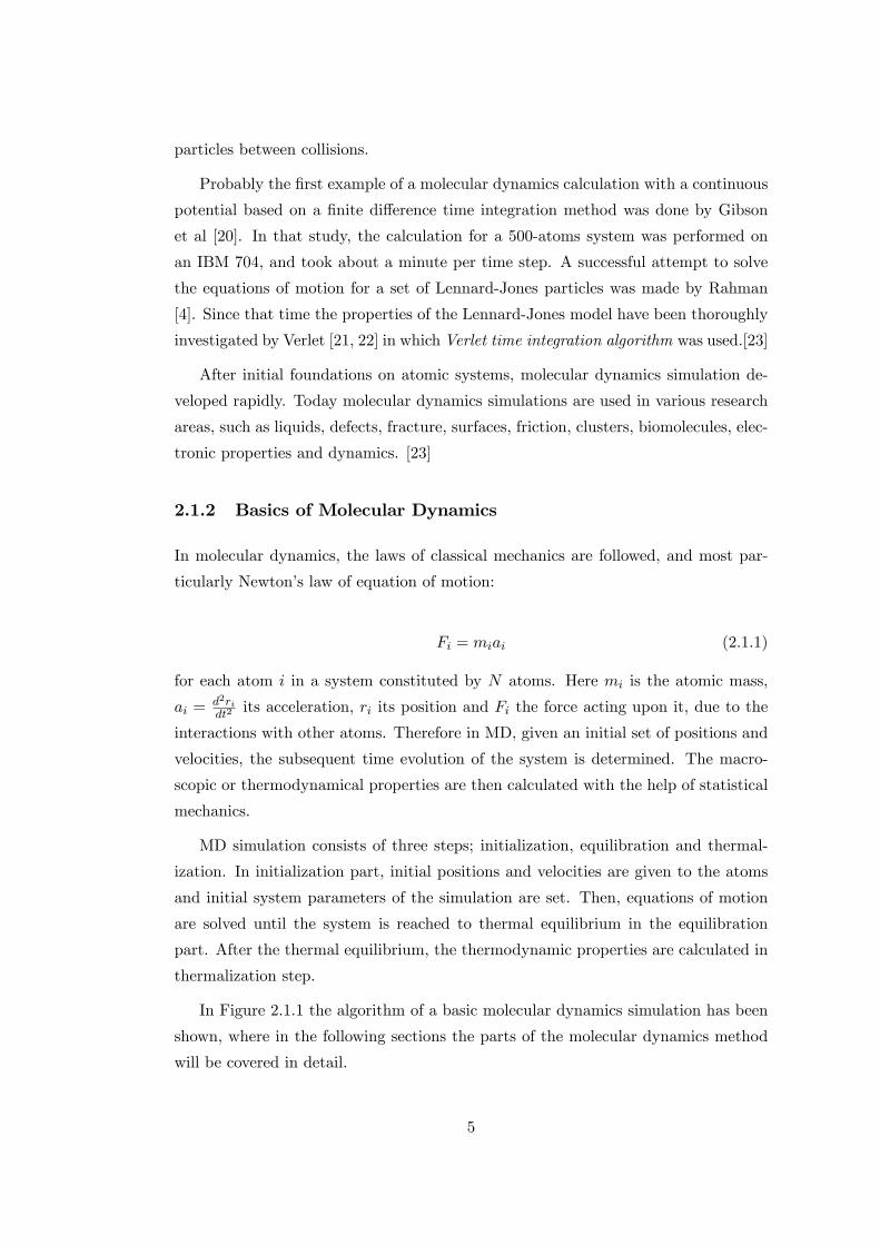
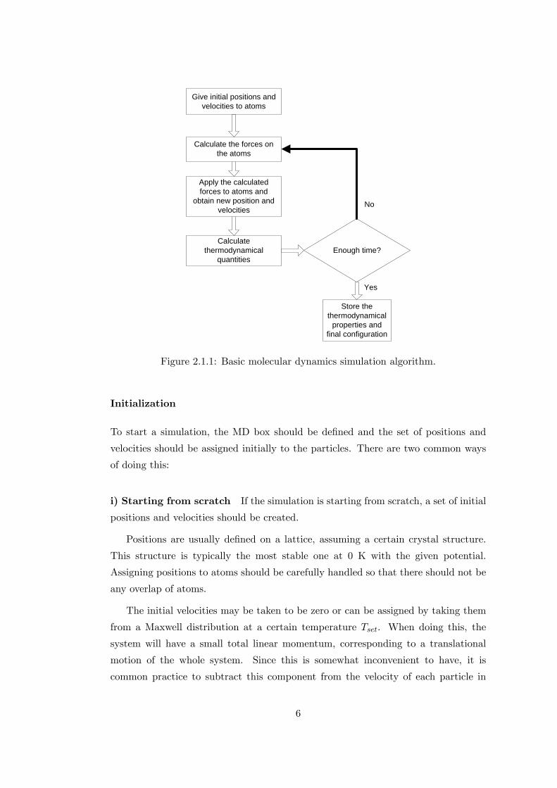
MD simulation consists of three steps; initialization, equilibration and thermal-

ization. In initialization part, initial positions and velocities are given to the atoms

and initial system parameters of the simulation are set. Then, equations of motion

are solved until the system is reached to thermal equilibrium in the equilibration

part. After the thermal equilibrium, the thermodynamic properties are calculated in

thermalization step.

In Figure 2.1.1 the algorithm of a basic molecular dynamics simulation has been

shown, where in the following sections the parts of the molecular dynamics method

will be covered in detail.

5

Give initial positions andvelocities to atoms

Calculate the forces onthe atoms

Apply the calculatedforces to atoms and

obtain new position andvelocities

Calculatethermodynamical

quantitiesEnough time?

Store thethermodynamical

properties andfinal configuration

No

Yes

Figure 2.1.1: Basic molecular dynamics simulation algorithm.

Initialization

To start a simulation, the MD box should be de�ned and the set of positions and

velocities should be assigned initially to the particles. There are two common ways

of doing this:

i) Starting from scratch If the simulation is starting from scratch, a set of initial

positions and velocities should be created.

Positions are usually de�ned on a lattice, assuming a certain crystal structure.

This structure is typically the most stable one at 0 K with the given potential.

Assigning positions to atoms should be carefully handled so that there should not be

any overlap of atoms.

The initial velocities may be taken to be zero or can be assigned by taking them

from a Maxwell distribution at a certain temperature Tset. When doing this, the

system will have a small total linear momentum, corresponding to a translational

motion of the whole system. Since this is somewhat inconvenient to have, it is

common practice to subtract this component from the velocity of each particle in

6

order to operate in a zero total momentum condition. Initial temperature of the

system is also given in the initialization step by adjusting the kinetic energy. The

instantaneous temperature, T (t) of the system is given by the relation 2.1.2

NfkbT (t) =NXi=1

miv2i (2.1.2)

where Nf is the degrees of freedom (Nf = 3N � 3 for a system of N particles with

zero total linear momentum), kb is the Boltzmann constant and vi is the velocity on

atom i. The right hand side of Equation 2.1.2 is two times of the average kinetic

energy. This equation comes from the equipartition principle [24]: an average energy

of kbT=2 per degree of freedom. The desired temperature, Tset, is obtained by scaling

all velocities with a factor (Tset=T (t))1=2 .

Such an initial state will not of course correspond to an equilibrium condition.

However, once the run is started, depending on the system size, equilibrium is usually

reached within a time of the order of several hundred time steps.

ii) Continuing a simulation Another possibility is to take the initial positions

and velocities to be the �nal positions and velocities of a previous MD run. This is

in fact the most commonly used method in actual production. For instance, if one

has to take measurements at di¤erent temperatures, the standard procedure is to set

up a chain of runs, where the starting point at each temperature is taken to be the

�nal point at the preceding temperature (lower if we are heating, higher if we are

cooling).

Atomic Interactions

In order to estimate the force acting between atoms, it is necessary to take into

account the elementary components of the atom. With the normal concept of an

atom made up of a central nucleus and orbital electrons, when it interacts with an

another atom, if there were no orbital electrons the force between two nuclei would be

Coulombic. The forces holding together the nuclear components - neutrons, protons

- are of a completely di¤erent nature and orders of magnitude stronger than any

interatomic forces.

If atoms were considered as entities, there should be no forces between them at

distances greater than that at which they touch. However, at separations comparable

7

with the atomic diameter, the Coulomb interactions of the outer electrons of atom 1

with those of atom 2 and with the nucleus of atom 2 (and vice versa) have a signi�cant

e¤ect. The two atoms no longer view each other as entities and the interaction

becomes a rather complicated many-body problem.

Treatment of this many-body problem for all types of atomic interactions, re-

quires powerful computing systems. Fortunately, a number of approximations and

averaging procedures under di¤erent physical situations enable us to obtain analyti-

cal expressions or numerical values for the interatomic forces which may be applied

with varying degrees of con�dence to atomic problems [25].

For most purposes the force between two atoms is expressed in terms of their

potential energy of interaction, or interatomic potential. It depends to a �rst ap-

proximation on the separation r between the atoms; the relation between the force

F (r) and the potential V (r) is

F (r) = �( @@r)V (r) (2.1.3)

The potential energy of an atom is the work done in bringing all components of

the atom from in�nity to their equilibrium positions. The potential energy baseline

then is that of a system with the nucleus already fully constituted. The work required

to attach the atomic electrons to the nucleus under the force �elds of the nucleus and

of each other [25]. The potential energy V (r), representing non-bonded interactions

between atoms is traditionally split into 1-body, 2-body, 3- body,... terms;

V (rN ) =Xi

u(ri) +Xi

Xj>i

'(ri; rj) + ::: (2.1.4)

where rN = (r1; r2; :::rN ) represents the complete set of 3N coordinates. The u(r)

term in Equation 2.1.4 represents an externally applied potential �eld or the e¤ects of

the container walls; it is usually dropped for fully periodic simulations of bulk systems

[26]. Also it is usual to concentrate on the pair potential '(ri; rj) and neglect three

body and higher order interactions. There is an extensive literature on the way

these potentials are determined experimentally, or modelled theoretically [25]. In

some simulations of complex �uids, it is su¢ cient to use the simplest models that

faithfully represent the essential physics.

8

Integration of the Equations of Motion

The engine of a molecular dynamics program is its time integration algorithm, re-

quired to integrate the equation of motion of the interacting particles. The integrator

is responsible for the accuracy of the simulation results. Sutmann [5] summarized

the requirements of an integrator, such that an integrator should be accurate to ob-

tain a true trajectory, stable in the sense that it conserves energy and that small

perturbations do not lead to instabilities. An integrator should also be robust that

it permits a large time step to be used in order to propagate the system e¢ ciently

through phase space.

Time integration algorithms are based on �nite di¤erence methods, where time is

discretized on a �nite grid, the time step �t being the distance between consecutive

points on the grid [23]. Knowing the positions and some of their time derivatives

at time t, the integration scheme gives the same quantities at a later time t + �t.

By iterating the procedure, the time evolution of the system can be followed for

long times. Generally integration algorithms are based on Taylor expansion of po-

sitions and velocities. Some of the common integrators used in molecular dynamics

simulations are described in the following sections.

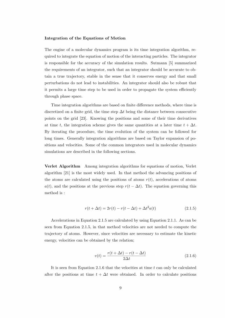
Verlet Algorithm Among integration algorithms for equations of motion, Verlet

algorithm [21] is the most widely used. In that method the advancing positions of

the atoms are calculated using the positions of atoms r(t), accelerations of atoms

a(t), and the positions at the previous step r(t ��t). The equation governing thismethod is :

r(t+�t) = 2r(t)� r(t��t) + �t2a(t) (2.1.5)

Accelerations in Equation 2.1.5 are calculated by using Equation 2.1.1. As can be

seen from Equation 2.1.5, in that method velocities are not needed to compute the

trajectory of atoms. However, since velocities are necessary to estimate the kinetic

energy, velocities can be obtained by the relation;

v(t) =r(t+�t)� r(t��t)

2�t(2.1.6)

It is seen from Equation 2.1.6 that the velocities at time t can only be calculated

after the positions at time t + �t were obtained. In order to calculate positions

9

and velocities at the same time, Verlet algorithm has been modi�ed [27] including

�leapfrog�[28] and �velocity Verlet�[29] form. In velocity Verlet scheme, positions and

velocities at t +�t are obtained from the same quantities at time t. The equations

of this method are:

r(t+�t) = r(t) + v(t)�t+1

2a(t)�t2 (2.1.7)

v(t+�t

2) = v(t) +

1

2a(t)�t (2.1.8)

a(t+�t) = � 1mrV (r(t+�t)) (2.1.9)

v(t+�t) = v(t+�t

2) +

1

2a(t+�t)�t (2.1.10)

The error associated to the velocity - Verlet method is of order �t4 where, original

Verlet has an error, order of �t2. Velocity Verlet form of the integrator resembles a

three-value predictor-corrector algorithm where the position coe¢ cient is zero [26].

Predictor-corrector Algorithm Predictor-corrector algorithms commonly used

to integrate the equations of motion used in molecular dynamics are due to Gear

[30, 31], and consists of three steps [23]:

1. Predictor: The positions and their time derivatives up to a certain order q

are predicted at time t + �t using their current values by means of a Taylor

expansion.

2. Force evaluation: The force is computed by Equation 2.1.3 using the predicted

positions.

3. Corrector: The di¤erence between the accelerations calculated from force eval-

uation and predicted accelerations is used to correct positions and their deriv-

atives. All the corrections are proportional to the error signal, the coe¢ cient

of proportionality being a magic number determined to maximize the stability

of the algorithm.

10

In the predictor part, the estimate of positions, velocities, accelerations, etc. at

time t + �t is obtained by Taylor expansion at time t. For the �fth order Gear

predictor-corrector method the equations are written as:

rp(t+�t) = r(t) + v(t)�t+1

2a(t)�t2 +

1

6b(t)�t3 +

1

24c(t)�t4 (2.1.11)

vp(t+�t) = v(t) + a(t)�t+1

2b(t)�t2 +

1

6c(t)�t3

ap(t+�t) = a(t) + b(t)�t+1

2c(t)�t2

bp(t+�t) = b(t) + c(t)�t

The superscript p designate the predicted values. r, v, a, denotes the positions,

velocities and accelerations respectively and b and c are third and fourth derivatives

of r. The predicted equations given above do not give the true trajectory of atoms

since the equations of motion have not been introduced. The corrected accelerations,

ac(t+�t), are calculated using the new positions, rp, from the forces at time t+�t.

These corrected accelerations are then compared with the predicted values to estimate

the size of the error.

�a(t+�t) = ac(t+�t)� ap(t+�t) (2.1.12)

Using this error positions, velocities, etc. are corrected.

rc(t+�t) = rp(t+�t) + c0�a(t+�t) (2.1.13)

vc(t+�t) = vp(t+�t) + c1�a(t+�t)

ac(t+�t) = ap(t+�t) + c2�a(t+�t)

bc(t+�t) = bp(t+�t) + c3�a(t+�t)

cc(t+�t) = cp(t+�t) + c4�a(t+�t)

where the superscript c donates the corrected values and c0, c1, c2, c3, c4 are the

parameters suggested by Gear [30, 31]. These parameters are given in Table 2.1.1.

11

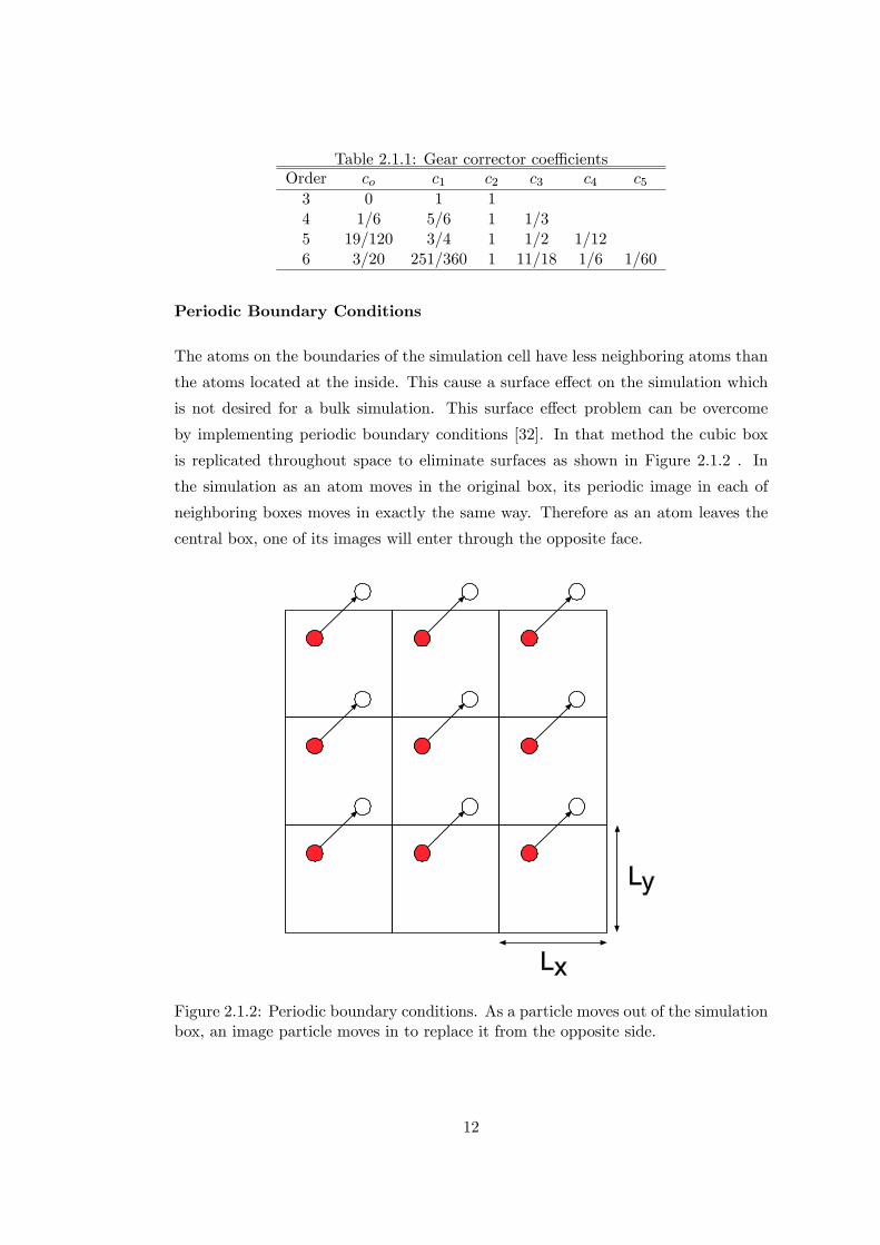
Table 2.1.1: Gear corrector coe¢ cientsOrder co c1 c2 c3 c4 c53 0 1 14 1=6 5=6 1 1=35 19=120 3=4 1 1=2 1=126 3=20 251=360 1 11=18 1=6 1=60

Periodic Boundary Conditions

The atoms on the boundaries of the simulation cell have less neighboring atoms than

the atoms located at the inside. This cause a surface e¤ect on the simulation which

is not desired for a bulk simulation. This surface e¤ect problem can be overcome

by implementing periodic boundary conditions [32]. In that method the cubic box

is replicated throughout space to eliminate surfaces as shown in Figure 2.1.2 . In

the simulation as an atom moves in the original box, its periodic image in each of

neighboring boxes moves in exactly the same way. Therefore as an atom leaves the

central box, one of its images will enter through the opposite face.

Figure 2.1.2: Periodic boundary conditions. As a particle moves out of the simulationbox, an image particle moves in to replace it from the opposite side.

12

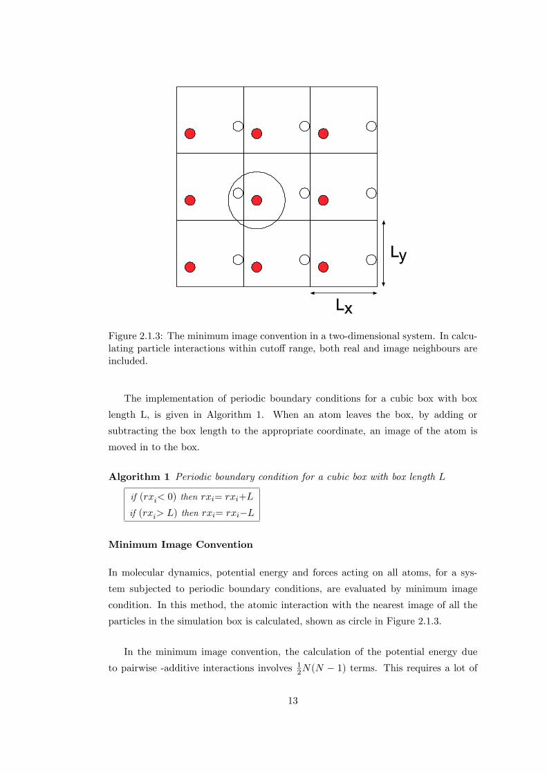
Figure 2.1.3: The minimum image convention in a two-dimensional system. In calcu-lating particle interactions within cuto¤ range, both real and image neighbours areincluded.

The implementation of periodic boundary conditions for a cubic box with box

length L, is given in Algorithm 1. When an atom leaves the box, by adding or

subtracting the box length to the appropriate coordinate, an image of the atom is

moved in to the box.

Algorithm 1 Periodic boundary condition for a cubic box with box length L

if (rxi< 0) then rxi= rxi+L

if (rxi> L) then rxi= rxi�L

Minimum Image Convention

In molecular dynamics, potential energy and forces acting on all atoms, for a sys-

tem subjected to periodic boundary conditions, are evaluated by minimum image

condition. In this method, the atomic interaction with the nearest image of all the

particles in the simulation box is calculated, shown as circle in Figure 2.1.3.

In the minimum image convention, the calculation of the potential energy due

to pairwise -additive interactions involves 12N(N � 1) terms. This requires a lot of

13

computation time even for small systems. The largest contribution to the potential

and forces come from the neighbors close to the atom of interest, and for short-range

forces generally a spherical cuto¤ is applied. With a cuto¤ distance rc, the pair

potential '(r) is set to zero for r � rc. The cuto¤ distance should be large enoughto minimize the perturbation because of the use of cuto¤. The cut o¤ distance

should be less than L2 for consistency with the minimum image convention [26].

The implementation of minimum image convention is similar to periodic boundary

conditions as can be seen in Figure 2.1.3. In the given Algorithm 2, rxij is the

interatomic separation of atoms in interest with the cubic simulation box length L.

Algorithm 2 Minimum image convention for a cubic box with box length L

if (rxij< �L=2) then rxij= rxij + Lif (rxij> L=2) then rxij= rxij � L

Linked List

In the evaluation of forces and potential energy for an atom all of the minimum image

distances are calculated and if the pairs are separated greater than a potential cuto¤,

the evaluation process is not carried out. If the system size increases towards 1000

atoms, this evaluation sequence becomes very time consuming. To avoid the needless

calculation of pair separations that are so large, linked list algorithm can be used.

In this method at �rst, the simulation box, L, is divided into M �M �M small

cells of equal size. The dimensions of the cell, l = LM should be greater than the

cuto¤ distance, rc. An atom in a cell interacts with only the other atoms in the same

cell and its 26 neighbor cells.

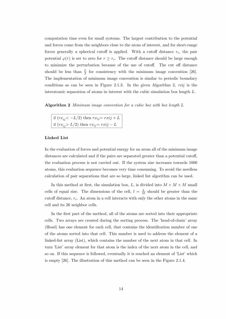
In the �rst part of the method, all of the atoms are sorted into their appropriate

cells. Two arrays are created during the sorting process. The �head-of-chain�array

(Head) has one element for each cell, that contains the identi�cation number of one

of the atoms sorted into that cell. This number is used to address the element of a

linked-list array (List), which contains the number of the next atom in that cell. In

turn �List�array element for that atom is the index of the next atom in the cell, and

so on. If this sequence is followed, eventually it is reached an element of �List�which

is empty [26]. The illustration of this method can be seen in the Figure 2.1.4.

14

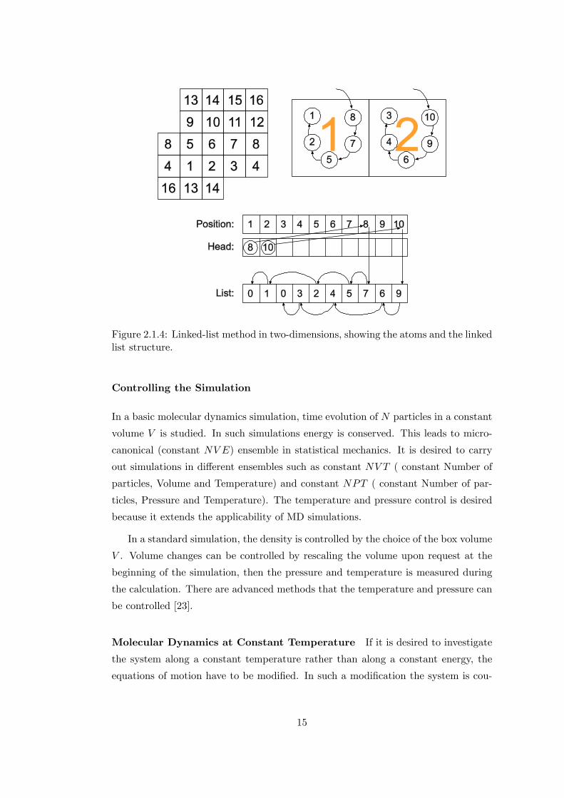
Figure 2.1.4: Linked-list method in two-dimensions, showing the atoms and the linkedlist structure.

Controlling the Simulation

In a basic molecular dynamics simulation, time evolution of N particles in a constant

volume V is studied. In such simulations energy is conserved. This leads to micro-

canonical (constant NV E) ensemble in statistical mechanics. It is desired to carry

out simulations in di¤erent ensembles such as constant NV T ( constant Number of

particles, Volume and Temperature) and constant NPT ( constant Number of par-

ticles, Pressure and Temperature). The temperature and pressure control is desired

because it extends the applicability of MD simulations.

In a standard simulation, the density is controlled by the choice of the box volume

V . Volume changes can be controlled by rescaling the volume upon request at the

beginning of the simulation, then the pressure and temperature is measured during

the calculation. There are advanced methods that the temperature and pressure can

be controlled [23].

Molecular Dynamics at Constant Temperature If it is desired to investigate

the system along a constant temperature rather than along a constant energy, the

equations of motion have to be modi�ed. In such a modi�cation the system is cou-

15

pled to a heat bath, which introduces energy �uctuations necessary to keep a �xed

temperature. Equilibrium of a system in a heat bath is a representative of canonical

ensemble, where the number of particles N , the volume V , and the temperature T ,

are �xed and there is zero total linear momentum [33]. Although the total energy is

not conserved in constant temperature simulations, average kinetic energy is a con-

stant of motion due to its coupling with the temperature. In such a modi�cation

since the total energy is not conserved, important data is not collected in this stage.

The controlled temperature simulations are used only to bring the system from one

state to the other. Data collection is carried out after the system has reached equilib-

rium. There are various methods which are discussed separately in the accompanying

sections, to �x the temperature to a �xed value during simulation.

Velocity Scaling In velocity scaling which is introduced by Woodcock [34],

temperature is adjusted to the desired value by rescaling the velocities with a factor

�. The scaling factor � is given in Equation 2.1.14.

� =

2664(3N � 4)kbTsetXi

mv2i

37751=2

(2.1.14)

In Equation 2.1.14, Tset is the desired temperature and degrees of freedom is used

as 3N � 4, instead of 3N . The system has 3N degrees of freedom, because of zero

total momentum in all directions, three degrees of freedom is removed and constant

kinetic energy removes one degree of freedom.

Algorithm 3 NV T molecular dynamics algorithm with velocity scaling

do t = 0; totstep start of MD loop

r(t+�t) = r(t) + v(t)�t+12a(t)�t

2 calculate new positions

v(t+�t2 ) = v(t)+

12a(t)�t calculate velocities at half step

a(t+�t) = � 1mrV (r(t+�t)) evaluate force using new positions

v(t+�t) = v(t+�t2 )+

12a(t+�t)�t update velocities

K =12mv(t+�t)

2 calculate kinetic energy

� = [(3N � 4)kbTset=2K]1=2 calculate the scale factor

v(t+�t) = v(t+�t)� scale velocities

end do

16

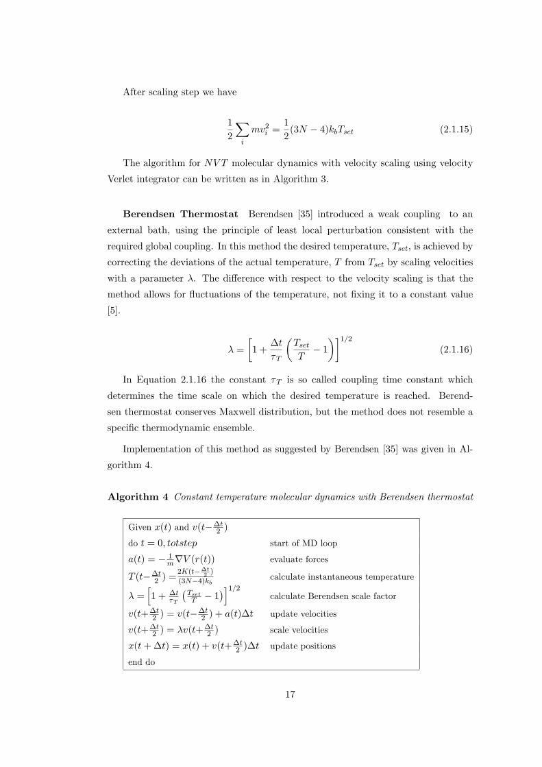
After scaling step we have

1

2

Xi

mv2i =1

2(3N � 4)kbTset (2.1.15)

The algorithm for NV T molecular dynamics with velocity scaling using velocity

Verlet integrator can be written as in Algorithm 3.

Berendsen Thermostat Berendsen [35] introduced a weak coupling to an

external bath, using the principle of least local perturbation consistent with the

required global coupling. In this method the desired temperature, Tset, is achieved by

correcting the deviations of the actual temperature, T from Tset by scaling velocities

with a parameter �. The di¤erence with respect to the velocity scaling is that the

method allows for �uctuations of the temperature, not �xing it to a constant value

[5].

� =

�1 +

�t

�T

�TsetT

� 1��1=2

(2.1.16)

In Equation 2.1.16 the constant �T is so called coupling time constant which

determines the time scale on which the desired temperature is reached. Berend-

sen thermostat conserves Maxwell distribution, but the method does not resemble a

speci�c thermodynamic ensemble.

Implementation of this method as suggested by Berendsen [35] was given in Al-

gorithm 4.

Algorithm 4 Constant temperature molecular dynamics with Berendsen thermostat

Given x(t) and v(t��t2 )

do t = 0; totstep start of MD loop

a(t) = � 1mrV (r(t)) evaluate forces

T (t��t2 ) =

2K(t��t2)

(3N�4)kb calculate instantaneous temperature

� =h1 + �t

�T

�TsetT � 1

�i1=2calculate Berendsen scale factor

v(t+�t2 ) = v(t�

�t2 ) + a(t)�t update velocities

v(t+�t2 ) = �v(t+

�t2 ) scale velocities

x(t+�t) = x(t) + v(t+�t2 )�t update positions

end do

17

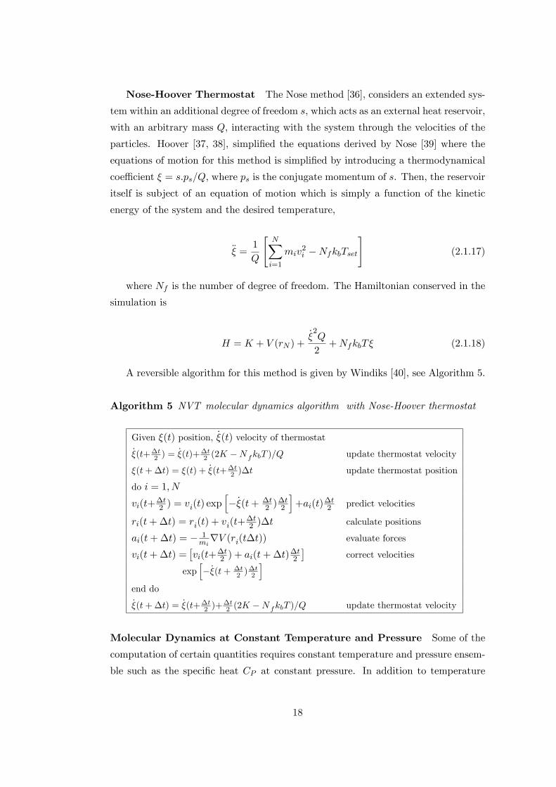
Nose-Hoover Thermostat The Nose method [36], considers an extended sys-

tem within an additional degree of freedom s, which acts as an external heat reservoir,

with an arbitrary mass Q, interacting with the system through the velocities of the

particles. Hoover [37, 38], simpli�ed the equations derived by Nose [39] where the

equations of motion for this method is simpli�ed by introducing a thermodynamical

coe¢ cient � = s:ps=Q; where ps is the conjugate momentum of s. Then, the reservoir

itself is subject of an equation of motion which is simply a function of the kinetic

energy of the system and the desired temperature,

�� =1

Q

"NXi=1

miv2i �NfkbTset

#(2.1.17)

where Nf is the number of degree of freedom. The Hamiltonian conserved in the

simulation is

H = K + V (rN ) +_�2Q

2+NfkbT� (2.1.18)

A reversible algorithm for this method is given by Windiks [40], see Algorithm 5.

Algorithm 5 NVT molecular dynamics algorithm with Nose-Hoover thermostat

Given �(t) position, _�(t) velocity of thermostat

_�(t+�t2 ) =

_�(t)+�t2 (2K �NfkbT )=Q update thermostat velocity

�(t+�t) = �(t) + _�(t+�t2 )�t update thermostat position

do i = 1; N

vi(t+�t2 ) = vi(t) exp

h� _�(t+ �t

2 )�t2

i+ai(t)

�t2 predict velocities

ri(t+�t) = ri(t) + vi(t+�t2 )�t calculate positions

ai(t+�t) = � 1mirV (ri(t�t)) evaluate forces

vi(t+�t) =�vi(t+

�t2 ) + ai(t+�t)

�t2

�correct velocities

exph� _�(t+ �t

2 )�t2

iend do

_�(t+�t) = _�(t+�t2 )+

�t2 (2K �NfkbT )=Q update thermostat velocity

Molecular Dynamics at Constant Temperature and Pressure Some of the

computation of certain quantities requires constant temperature and pressure ensem-

ble such as the speci�c heat CP at constant pressure. In addition to temperature

18

control, which is discussed in the previous section, if it is desired also to �x the pres-

sure to a constant value, then the volume must be allowed to �uctuate [33]. Two

common methods for this ensemble is discovered by Andersen and Berendsen, which

are discussed in the following sections.

Andersen Method A summary of this method was given by Allen and Tildes-

ley [26]. Andersen [41] introduced a method for controlling the pressure in molecular

dynamics which involves coupling the system to an external variable V , the volume

of the simulation box. This coupling act as a piston on a real system. The piston

has a mass Q with kinetic energy

KV =1

2Q _V 2 (2.1.19)

The potential energy associated with the additional variable is

VV = PV (2.1.20)

where P is the speci�ed pressure. In this method r and V are not coupled. The

coordinates ri of particles are replaced with the scaled coordinates �i.

�i = ri=V1=3 (2.1.21)

The equations of motion of the system are

�� =F

mV 1=3� 2 _�

_V

3V(2.1.22)

�V =(P � Pset)

Q(2.1.23)

where Q is the piston mass, P is the instantaneous pressure, which can be calculated

from the virial equation that is to be explained later (see Equation 2.1.32) and Pset

is the desired pressure. The algorithm of this method was given in Algorithm 6.

Haile and Graben [42] described a way of implementing this method, solving the

equations of motion in terms of the scaled positions and momenta in a box of unit

length using a Gear predictor-corrector integrator.

The parameter Q, the piston mass, can be adjusted. A low mass results in rapid

19

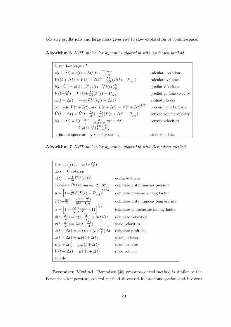
box size oscillations and large mass gives rise to slow exploration of volume-space.

Algorithm 6 NPT molecular dynamics algorithm with Andersen method

Given box length L

�(t+�t) = �(t) + �t _�(t)+�t2a(t)2L(t) calculate positions

V ((t+�t) = V (t) + �t _V+�t2

2Q (P (t)� P set) calculate volume

_�(t+�t2 ) = _�(t)+ �t

2L(t)a(t)��t2 _�(t)

_V (t)V (t) predict velocities

_V (t+�t2 ) =

_V (t)+�t2Q(P (t)� P set) predict volume velocity

ai(t+�t) = � 1mirV (ri(t+�t)) evaluate forces

compute P (t+�t), and L(t+�t) = V (t+�t)1=3 pressure and box size

_V (t+�t) = _V (t+�t2 )+

�t2Q(P (t+�t)� P set) correct volume velocity

_�(t+�t) = _�(t+�t2 )+

�t2L(t+�t)a(t+�t) correct velocities

��t2 _�(t+

�t2 )

_V (t+�t2 )

V (t+�t)

adjust temperature by velocity scaling scale velocities

Algorithm 7 NPT molecular dynamics algorithm with Berendsen method

Given x(t) and v(t��t2 )

do t = 0; totstep

a(t) = � 1mrV (r(t)) evaluate forces

calculate P (t) from eq. 2.1.32 calculate instantaneous pressure

� =h1+�t

�P�(P (t)� P set)

i1=3calculate pressure scaling factor

T (t��t2 ) =

2K(t��t2)

(3N�4)kb calculate instantaneous temperature

� =h1 + �t

�T

�TsetT � 1

�i1=2calculate temperature scaling factor

v(t+�t2 ) = v(t�

�t2 ) + a(t)�t calculate velocities

v(t+�t2 ) = �v(t+

�t2 ) scale velocities

x(t+�t) = x(t) + v(t+�t2 )�t calculate positions

x(t+�t) = �x(t+�t) scale positions

L(t+�t) = �L(t+�t) scale box size

V (t+�t) = �V (t+�t) scale volume

end do

Berendsen Method Berendsen [35] pressure control method is similar to the

Berendsen temperature control method discussed in previous section and involves

20

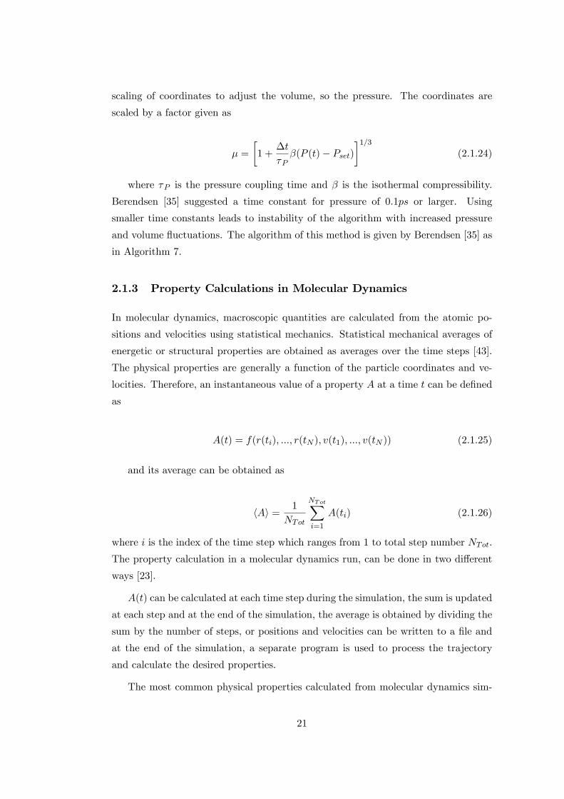
scaling of coordinates to adjust the volume, so the pressure. The coordinates are

scaled by a factor given as

� =

�1 +

�t

�P�(P (t)� Pset)

�1=3(2.1.24)

where �P is the pressure coupling time and � is the isothermal compressibility.

Berendsen [35] suggested a time constant for pressure of 0:1ps or larger. Using

smaller time constants leads to instability of the algorithm with increased pressure

and volume �uctuations. The algorithm of this method is given by Berendsen [35] as

in Algorithm 7.

2.1.3 Property Calculations in Molecular Dynamics

In molecular dynamics, macroscopic quantities are calculated from the atomic po-

sitions and velocities using statistical mechanics. Statistical mechanical averages of

energetic or structural properties are obtained as averages over the time steps [43].

The physical properties are generally a function of the particle coordinates and ve-

locities. Therefore, an instantaneous value of a property A at a time t can be de�ned

as

A(t) = f(r(ti); :::; r(tN ); v(t1); :::; v(tN )) (2.1.25)

and its average can be obtained as

hAi = 1

NTot

NTotXi=1

A(ti) (2.1.26)

where i is the index of the time step which ranges from 1 to total step number NTot.

The property calculation in a molecular dynamics run, can be done in two di¤erent

ways [23].

A(t) can be calculated at each time step during the simulation, the sum is updated

at each step and at the end of the simulation, the average is obtained by dividing the

sum by the number of steps, or positions and velocities can be written to a �le and

at the end of the simulation, a separate program is used to process the trajectory

and calculate the desired properties.

The most common physical properties calculated from molecular dynamics sim-

21

ulations are discussed in the following sections.

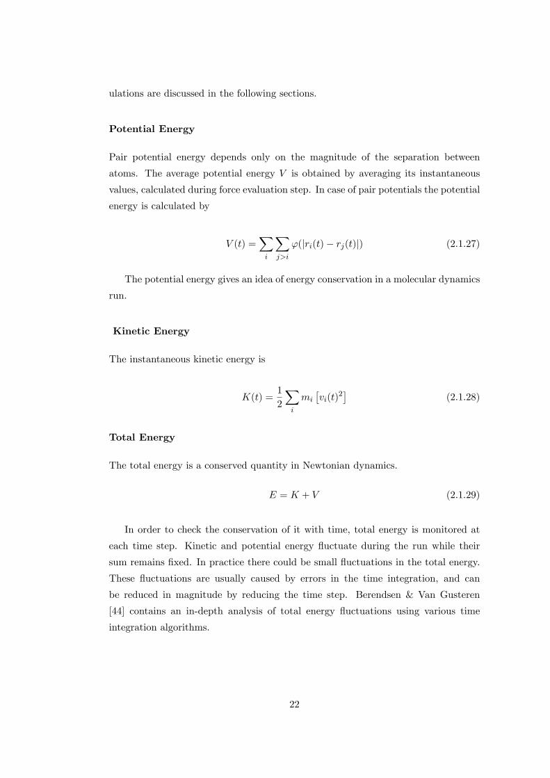
Potential Energy

Pair potential energy depends only on the magnitude of the separation between

atoms. The average potential energy V is obtained by averaging its instantaneous

values, calculated during force evaluation step. In case of pair potentials the potential

energy is calculated by

V (t) =Xi

Xj>i

'(jri(t)� rj(t)j) (2.1.27)

The potential energy gives an idea of energy conservation in a molecular dynamics

run.

Kinetic Energy

The instantaneous kinetic energy is

K(t) =1

2

Xi

mi

�vi(t)

2�

(2.1.28)

Total Energy

The total energy is a conserved quantity in Newtonian dynamics.

E = K + V (2.1.29)

In order to check the conservation of it with time, total energy is monitored at

each time step. Kinetic and potential energy �uctuate during the run while their

sum remains �xed. In practice there could be small �uctuations in the total energy.

These �uctuations are usually caused by errors in the time integration, and can

be reduced in magnitude by reducing the time step. Berendsen & Van Gusteren

[44] contains an in-depth analysis of total energy �uctuations using various time

integration algorithms.

22

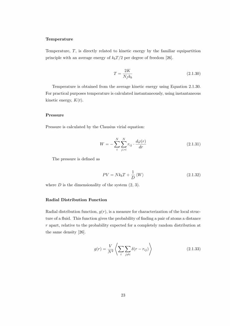
Temperature

Temperature, T , is directly related to kinetic energy by the familiar equipartition

principle with an average energy of kbT=2 per degree of freedom [26].

T =2K

Nfkb(2.1.30)

Temperature is obtained from the average kinetic energy using Equation 2.1.30.

For practical purposes temperature is calculated instantaneously, using instantaneous

kinetic energy, K(t).

Pressure

Pressure is calculated by the Clausius virial equation:

W = �NXi

NXj>i

rij �d'(r)

dr(2.1.31)

The pressure is de�ned as

PV = NkbT +1

DhW i (2.1.32)

where D is the dimensionality of the system (2, 3).

Radial Distribution Function

Radial distribution function, g(r), is a measure for characterization of the local struc-

ture of a �uid. This function gives the probability of �nding a pair of atoms a distance

r apart, relative to the probability expected for a completely random distribution at

the same density [26].

g(r) =V

N2

*Xi

Xj 6=i

�(r � rij)+

(2.1.33)

23

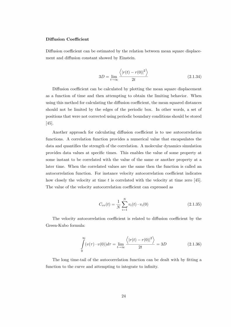
Di¤usion Coe¢ cient

Di¤usion coe¢ cient can be estimated by the relation between mean square displace-

ment and di¤usion constant showed by Einstein.

3D = limt!1

Djr(t)� r(0)j2

E2t

(2.1.34)

Di¤usion coe¢ cient can be calculated by plotting the mean square displacement

as a function of time and then attempting to obtain the limiting behavior. When

using this method for calculating the di¤usion coe¢ cient, the mean squared distances

should not be limited by the edges of the periodic box. In other words, a set of

positions that were not corrected using periodic boundary conditions should be stored

[45].

Another approach for calculating di¤usion coe¢ cient is to use autocorrelation

functions. A correlation function provides a numerical value that encapsulates the

data and quanti�es the strength of the correlation. A molecular dynamics simulation

provides data values at speci�c times. This enables the value of some property at

some instant to be correlated with the value of the same or another property at a

later time. When the correlated values are the same then the function is called an

autocorrelation function. For instance velocity autocorrelation coe¢ cient indicates

how closely the velocity at time t is correlated with the velocity at time zero [45].

The value of the velocity autocorrelation coe¢ cient can expressed as

Cvv(t) =1

N

NXi=1

vi(t) � vi(0) (2.1.35)

The velocity autocorrelation coe¢ cient is related to di¤usion coe¢ cient by the

Green-Kubo formula:

1Z0

(v(�) � v(0))d� = limt!1

Djr(t)� r(0)j2

E2t

= 3D (2.1.36)

The long time-tail of the autocorrelation function can be dealt with by �tting a

function to the curve and attempting to integrate to in�nity.

24

2.2 Non-Equilibrium Molecular Dynamics

In the pervious section, the molecular dynamics simulation of systems under equilib-

rium conditions was considered. To improve the e¢ ciency of the calculation of the

transport properties and to examine directly the response of a system to a large per-

turbation real or imaginary using linear or nonlinear response theory, non-equilibrium

molecular dynamics (NEMD) simulations are carried out. This approach is �rstly in-

troduced by Hoover and Ashurst [8]. In equilibrium molecular dynamics, properties

represent the response to the naturally occurring small �uctuations. The signal-to-

noise ratio is not favorable at long times. In addition, the �nite system size limits

time that correlation functions can be calculated reliably in equilibrium molecular

dynamics (EMD) [26].

In contrast to EMD, NEMD introduce larger �uctuations arti�cially and the

signal-to-noise level of the measured response is higher. In addition to that the

steady state response is measured in NEMD. The calculations of transport properties

in NEMD are more realistic and give better results than EMD [26].

For the transport coe¢ cient of interest Lij , that is

Ji = LijXj (2.2.1)

where J is the �ux of some conserved quantity and X is a gradient in the density of

that conserved quantity, Green-Kubo relation will be

Lij =

Z 1

0hJi(t) � Jj(0)i dt (2.2.2)

Invent a �ctitious �eld Fe and its coupling to the system so that dissipative �ux

Jj holds

Had0 = �JjFe (2.2.3)

where Had0 is the added term to the Hamiltonian due to perturbation. The increase

in the Hamiltonian necessitates a thermostat, since otherwise, the work done on the

system would be transferred continuously into heat and no steady state could be

achieved. Then after the application of the thermostat, couple Fe to the system and

compute the steady state average hJi(t)i, as a function of the external �eld Fe.

25

Linear response theory then proves,

Lij = limFe!0

limt!1

hJi(t)iFe

This added an advantage to NEMD that it can be used to calculate non-linear

as well as linear transport coe¢ cients [9]. The application of NEMD methods to

calculate transport coe¢ cients is reviewed in detail by Evans and Morriss [46, 9] and

Allen and Tildesley [26].

The calculation of self di¤usion coe¢ cients with NEMD was illustrated by Er-

penbeck and Wood [47] for a system that exists a relation between susceptibility of

the color current to the magnitude of the perturbing color �eld with the velocity au-

tocorrelation function; where the di¤usion coe¢ cient can be written by Green-Kubo

relation as:

D =

Z 1

0dt hvi(t) � vi(0)i (2.2.4)

The color Hamiltonian of the system can be written as:

H = H0 �NXi=1

cixiF (t), t > 0 (2.2.5)

where H0 is the unperturbed Hamiltonian, ci are the color charges, and an even

number of atoms, N is considered with

ci = (�1)i (2.2.6)

The considered response is the color current density, Jx,

Jx =1

V

NXi=1

ci _xi (2.2.7)

Along with the lines of the above treatment and in the canonical ensemble,

hJx(t)Jx(0)ic =1

V 2

NXi;j

cicj hvxi(t)vxj(0)ic (2.2.8)

26

Upon further simpli�cation,

hJx(t)Jx(0)ic =1

V 2

NXi=1

c2i hvxi(t)vxi(0)ic =N

V 2hvx(t)vx(0)ic (2.2.9)

Combining Equation 2.2.9 with Green-Kubo relation for self di¤usion gives,

D =kbT

�limt!1

limF!0

hJx(t)iF

(2.2.10)

If the total linear momentum was set to zero for a system in consideration, then

vxi is not independent of vxj : Thus there is an order N�1 correction to this equation

and the self di¤usion coe¢ cient is obtained as

D =N � 1N

kbT

�limt!1

limF!0

hJx(t)iF

(2.2.11)

The advantage of this equation is that just with the simple average of color current

density, di¤usivity can be predicted. It is important to note that this di¤usivity does

not give any information about the di¤usion behavior under the applied force, since

from Equation 2.2.11, the di¤usivity is obtained when F ! 0: Thus the di¤usivity

obtained from this equation is the same as in the case when there is no applied force.

In addition, in binary alloys this treatment is not applicable.

27

Chapter 3

Potentials

The most important part of an atomistic simulation is the potential function which

describes the atomic interactions and the characteristic of the system. There are

various approaches to obtain the potential function. The potential function can be

obtained empirically, semi-emprically or from ab initio methods. Empirical poten-

tial functions are based on a simple analytical expression which may or may not

be justi�able from theory, and which contains one or more parameters adjusted to

an experimental situation [25]. Semi-empirical functions also contains parameters

�tted to an experimental value but analytical expressions are derived from quantum-

mechanical arguments.

Model pair potentials are derived within the pseudopotential context which are

�t to speci�c experimental characteristics of atoms or solids and are used to analyze

other physical characteristics or properties [48]. The application of pseudopotential

method to the interactions between atoms is covered in this chapter.

3.1 Pseudopotential theory

The determination of the properties of metals requires a knowledge of interaction

of electrons and ions. However, for many properties of materials, inner shell or

core electrons are not explicitly relevant to the properties of the materials, but the

valence electrons. The application of free-electron theory can be used to specify this

interaction, where the ion and electron interaction is considered to be very weak. In

contradiction with the free-electron theory, the ion core of a metal atom contains

strong force �elds which strongly a¤ects nearby electrons.

At the electrons nearby an ion core, the strong Coulomb attraction of the ion

28

core is opposed by the repulsion due to the operation of the Pauli principle for the

electrons of the closed shells. The net e¤ective interaction experienced by an electron,

as a result of the cancellation of the two principal contributions is quite small, and

this interaction is known as pseudopotential [25].

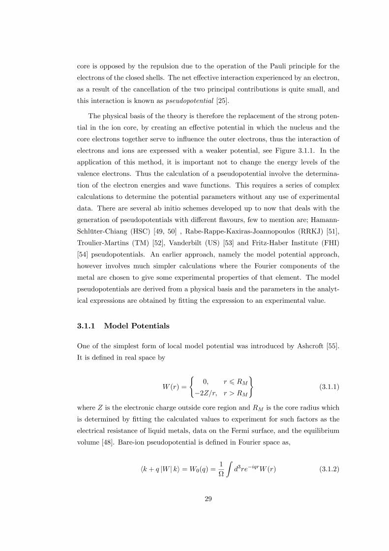
The physical basis of the theory is therefore the replacement of the strong poten-

tial in the ion core, by creating an e¤ective potential in which the nucleus and the

core electrons together serve to in�uence the outer electrons, thus the interaction of

electrons and ions are expressed with a weaker potential, see Figure 3.1.1. In the

application of this method, it is important not to change the energy levels of the

valence electrons. Thus the calculation of a pseudopotential involve the determina-

tion of the electron energies and wave functions. This requires a series of complex

calculations to determine the potential parameters without any use of experimental

data. There are several ab initio schemes developed up to now that deals with the

generation of pseudopotentials with di¤erent �avours, few to mention are; Hamann-

Schlüter-Chiang (HSC) [49, 50] , Rabe-Rappe-Kaxiras-Joannopoulos (RRKJ) [51],

Troulier-Martins (TM) [52], Vanderbilt (US) [53] and Fritz-Haber Institute (FHI)

[54] pseudopotentials. An earlier approach, namely the model potential approach,

however involves much simpler calculations where the Fourier components of the

metal are chosen to give some experimental properties of that element. The model

pseudopotentials are derived from a physical basis and the parameters in the analyt-

ical expressions are obtained by �tting the expression to an experimental value.

3.1.1 Model Potentials

One of the simplest form of local model potential was introduced by Ashcroft [55].

It is de�ned in real space by

W (r) =

(0; r 6 RM

�2Z=r; r > RM

)(3.1.1)

where Z is the electronic charge outside core region and RM is the core radius which

is determined by �tting the calculated values to experiment for such factors as the

electrical resistance of liquid metals, data on the Fermi surface, and the equilibrium

volume [48]. Bare-ion pseudopotential is de�ned in Fourier space as,

hk + q jW j ki =W0(q) =1

Zd3re�iqrW (r) (3.1.2)

29

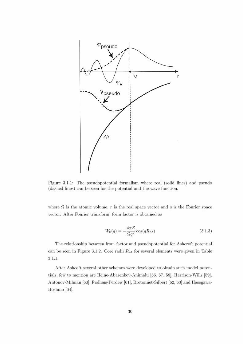
Figure 3.1.1: The pseudopotential formalism where real (solid lines) and pseudo(dashed lines) can be seen for the potential and the wave function.

where is the atomic volume, r is the real space vector and q is the Fourier space

vector. After Fourier transform, form factor is obtained as

W0(q) = �4�Z

q2cos(qRM ) (3.1.3)

The relationship between from factor and pseudopotential for Ashcroft potential

can be seen in Figure 3.1.2. Core radii RM for several elements were given in Table

3.1.1.

After Ashcoft several other schemes were developed to obtain such model poten-

tials, few to mention are Heine-Abarenkov-Animalu [56, 57, 58], Harrison-Wills [59],

Antonov-Milman [60], Fiolhais-Perdew [61], Bretonnet-Silbert [62, 63] and Hasegawa-

Hoshino [64].

30

W(r)

r

W(q)

qRM

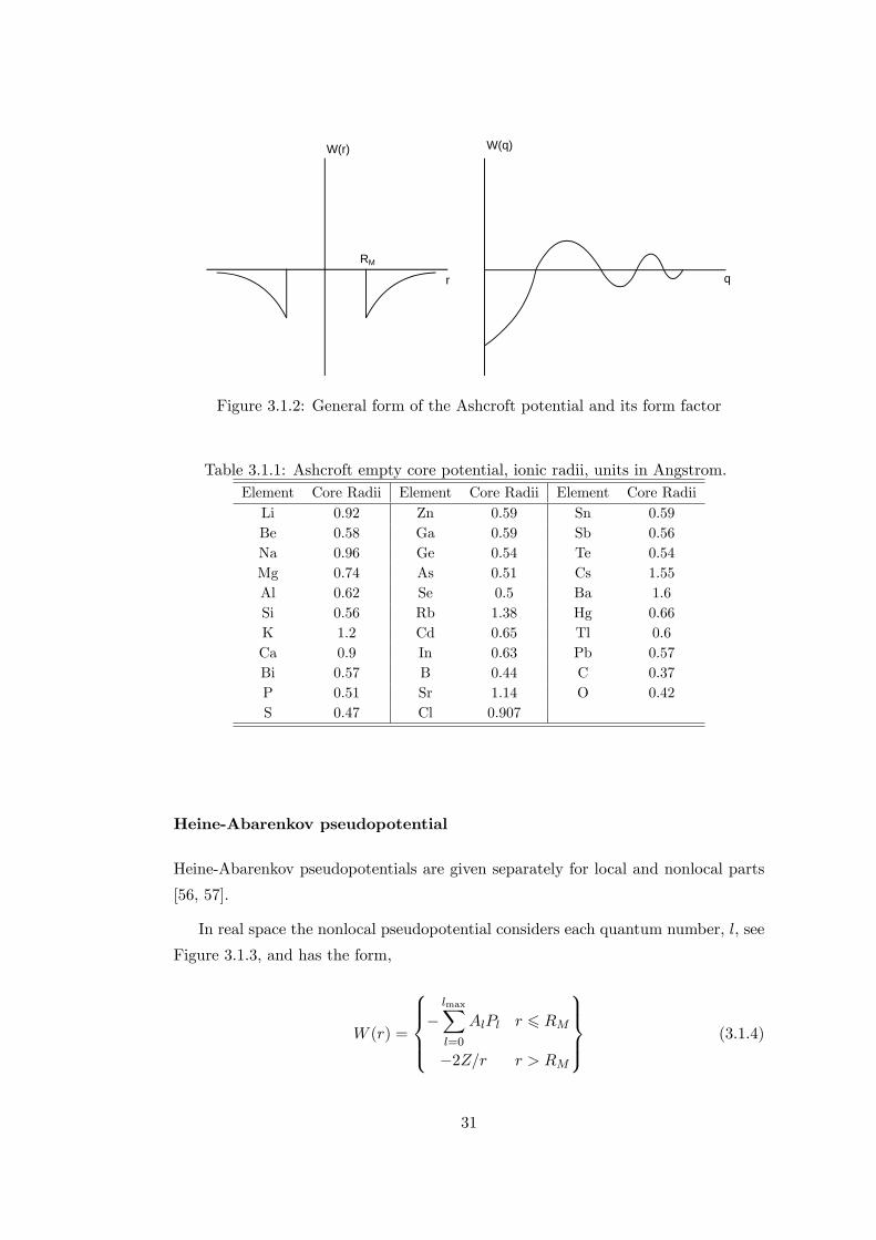
Figure 3.1.2: General form of the Ashcroft potential and its form factor

Table 3.1.1: Ashcroft empty core potential, ionic radii, units in Angstrom.Element Core Radii Element Core Radii Element Core RadiiLi 0.92 Zn 0.59 Sn 0.59Be 0.58 Ga 0.59 Sb 0.56Na 0.96 Ge 0.54 Te 0.54Mg 0.74 As 0.51 Cs 1.55Al 0.62 Se 0.5 Ba 1.6Si 0.56 Rb 1.38 Hg 0.66K 1.2 Cd 0.65 Tl 0.6Ca 0.9 In 0.63 Pb 0.57Bi 0.57 B 0.44 C 0.37P 0.51 Sr 1.14 O 0.42S 0.47 Cl 0.907

Heine-Abarenkov pseudopotential

Heine-Abarenkov pseudopotentials are given separately for local and nonlocal parts

[56, 57].

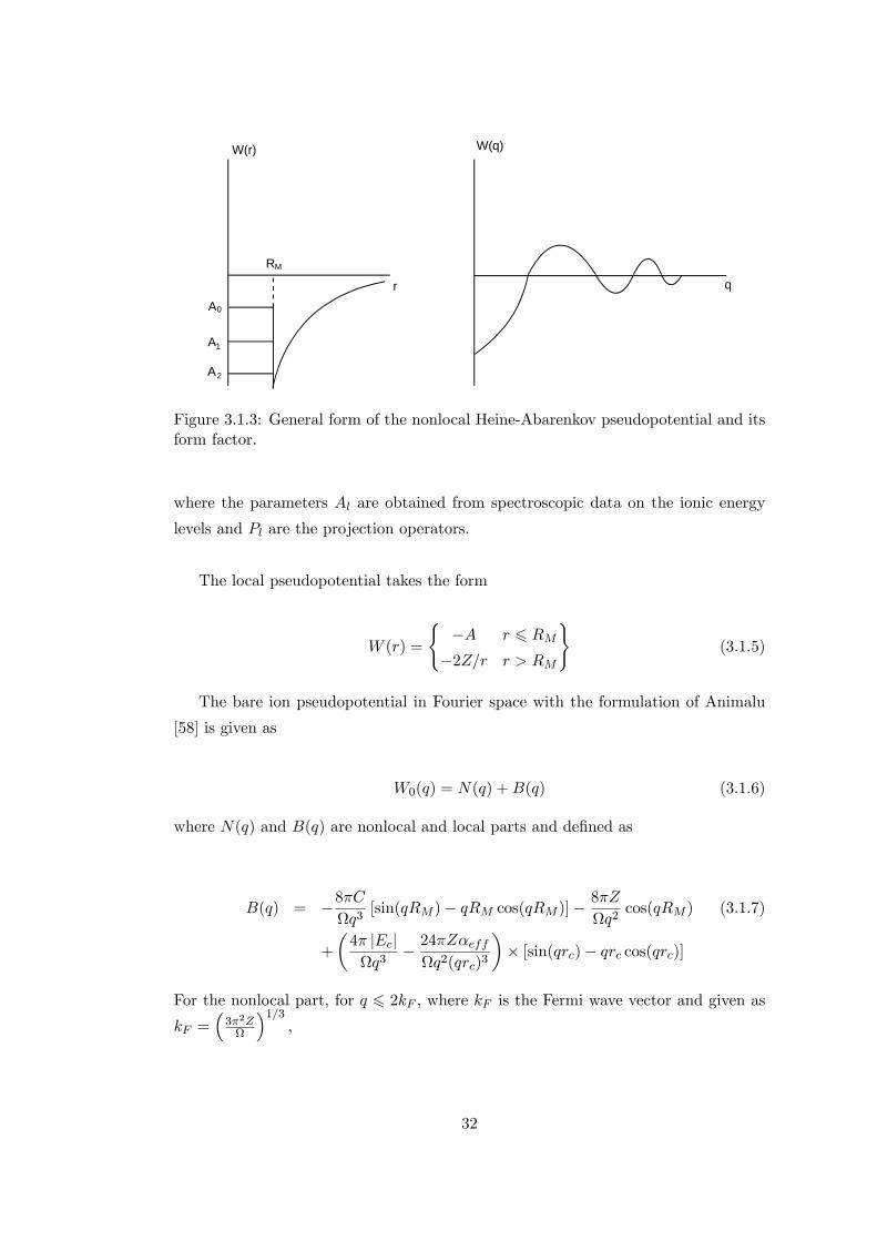
In real space the nonlocal pseudopotential considers each quantum number, l, see

Figure 3.1.3, and has the form,

W (r) =

8>><>>:�lmaxXl=0

AlPl r 6 RM

�2Z=r r > RM

9>>=>>; (3.1.4)

31

W(r)

r

W(q)

q

A

A

A

0

1

2

RM

Figure 3.1.3: General form of the nonlocal Heine-Abarenkov pseudopotential and itsform factor.

where the parameters Al are obtained from spectroscopic data on the ionic energy

levels and Pl are the projection operators.

The local pseudopotential takes the form

W (r) =

(�A r 6 RM�2Z=r r > RM

)(3.1.5)

The bare ion pseudopotential in Fourier space with the formulation of Animalu

[58] is given as

W0(q) = N(q) +B(q) (3.1.6)

where N(q) and B(q) are nonlocal and local parts and de�ned as

B(q) = �8�Cq3

[sin(qRM )� qRM cos(qRM )]�8�Z

q2cos(qRM ) (3.1.7)

+

�4� jEcjq3

� 24�Z�effq2(qrc)3

�� [sin(qrc)� qrc cos(qrc)]

For the nonlocal part, for q 6 2kF , where kF is the Fermi wave vector and given askF =

�3�2Z

�1=3;

32

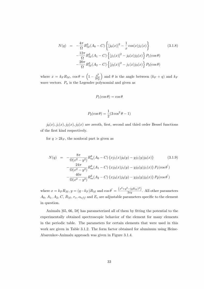
N(q) = �4�R3M (A0 � C)

�[j0(x)]

2 � 1

xcos(x)j1(x)

�(3.1.8)

�12�R3M (A1 � C)

n[j1(x)]

2 � j0(x)j2(x)oP1(cos �)

�20�R3M (A2 � C)

n[j2(x)]

2 � j1(x)j3(x)oP2(cos �)

where x = kFRM , cos � =�1� q2

2k2F

�and � is the angle between (kF + q) and kF

wave vectors. Pn is the Legendre polynomial and given as

P1(cos �) = cos �

P2(cos �) =1

2(3 cos2 � � 1)

j0(x); ji(x); j2(x); j3(x) are zeroth, �rst, second and third order Bessel functions

of the �rst kind respectively.

for q > 2kF , the nonlocal part is given as

N(q) = � 8�

(x2 � y2)R3m(A0 � C) fxj1(x)j0(y)� yj1(y)j0(x)g (3.1.9)

� 24�

(x2 � y2)R3m(A1 � C) fxj2(x)j1(y)� yj2(y)j1(x)gP1(cos �

0)

� 40�

(x2 � y2)R3m(A2 � C) fxj3(x)j2(y)� yj3(y)j2(x)gP2(cos �

0)

where x = kFRM , y = (q�kF )RM and cos �0=(x2+y2�(qRM )2)

2xy . All other parameters

A0, A1, A2, C, RM , rc, �eff and Ec are adjustable parameters speci�c to the element

in question.

Animalu [65, 66, 58] has parameterized all of them by �tting the potential to the

experimentally obtained spectroscopic behavior of the element for many elements

in the periodic table. The parameters for certain elements that were used in this

work are given in Table 3.1.2. The form factor obtained for aluminum using Heine-

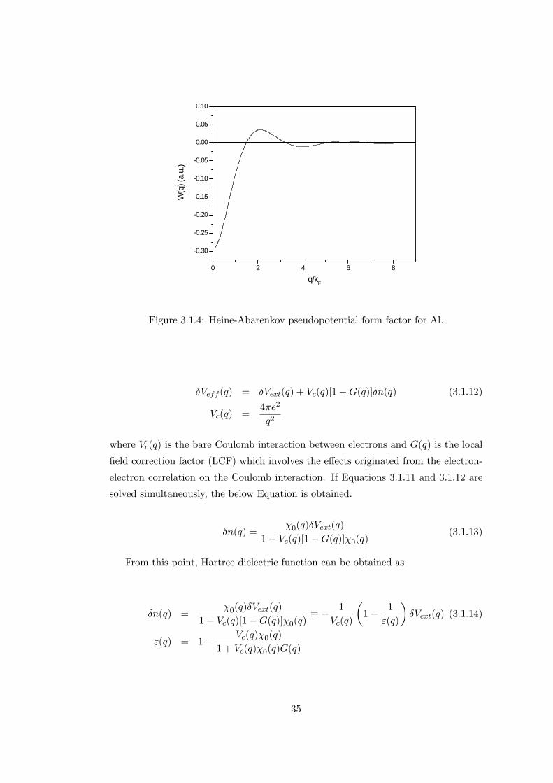
Abarenkov-Animalu approach was given in Figure 3.1.4.

33

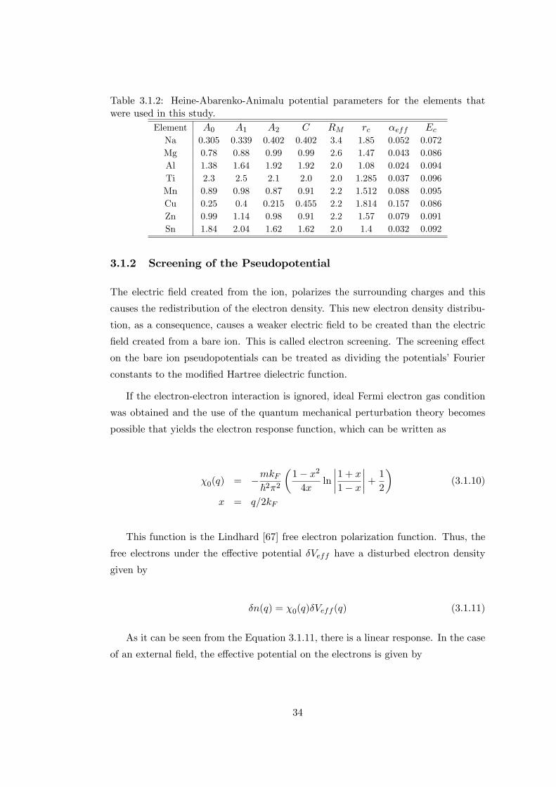
Table 3.1.2: Heine-Abarenko-Animalu potential parameters for the elements thatwere used in this study.

Element A0 A1 A2 C RM rc �eff EcNa 0.305 0.339 0.402 0.402 3.4 1.85 0.052 0.072Mg 0.78 0.88 0.99 0.99 2.6 1.47 0.043 0.086Al 1.38 1.64 1.92 1.92 2.0 1.08 0.024 0.094Ti 2.3 2.5 2.1 2.0 2.0 1.285 0.037 0.096Mn 0.89 0.98 0.87 0.91 2.2 1.512 0.088 0.095Cu 0.25 0.4 0.215 0.455 2.2 1.814 0.157 0.086Zn 0.99 1.14 0.98 0.91 2.2 1.57 0.079 0.091Sn 1.84 2.04 1.62 1.62 2.0 1.4 0.032 0.092

3.1.2 Screening of the Pseudopotential

The electric �eld created from the ion, polarizes the surrounding charges and this

causes the redistribution of the electron density. This new electron density distribu-

tion, as a consequence, causes a weaker electric �eld to be created than the electric

�eld created from a bare ion. This is called electron screening. The screening e¤ect

on the bare ion pseudopotentials can be treated as dividing the potentials�Fourier

constants to the modi�ed Hartree dielectric function.

If the electron-electron interaction is ignored, ideal Fermi electron gas condition

was obtained and the use of the quantum mechanical perturbation theory becomes

possible that yields the electron response function, which can be written as

�0(q) = �mkF~2�2

�1� x24x

ln

����1 + x1� x

����+ 12�

(3.1.10)

x = q=2kF

This function is the Lindhard [67] free electron polarization function. Thus, the

free electrons under the e¤ective potential �Veff have a disturbed electron density

given by

�n(q) = �0(q)�Veff (q) (3.1.11)

As it can be seen from the Equation 3.1.11, there is a linear response. In the case

of an external �eld, the e¤ective potential on the electrons is given by

34

0 2 4 6 8

­0.30

­0.25

­0.20

­0.15

­0.10

­0.05

0.00

0.05

0.10

W(q

) (a.

u.)

q/kF

Figure 3.1.4: Heine-Abarenkov pseudopotential form factor for Al.

�Veff (q) = �Vext(q) + Vc(q)[1�G(q)]�n(q) (3.1.12)

Vc(q) =4�e2

q2

where Vc(q) is the bare Coulomb interaction between electrons and G(q) is the local

�eld correction factor (LCF) which involves the e¤ects originated from the electron-

electron correlation on the Coulomb interaction. If Equations 3.1.11 and 3.1.12 are

solved simultaneously, the below Equation is obtained.

�n(q) =�0(q)�Vext(q)

1� Vc(q)[1�G(q)]�0(q)(3.1.13)

From this point, Hartree dielectric function can be obtained as

�n(q) =�0(q)�Vext(q)

1� Vc(q)[1�G(q)]�0(q)� � 1

Vc(q)

�1� 1

"(q)

��Vext(q) (3.1.14)

"(q) = 1� Vc(q)�0(q)

1 + Vc(q)�0(q)G(q)

35

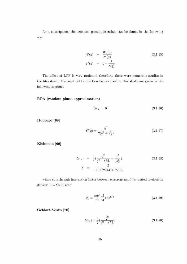
As a consequence the screened pseudopotentials can be found in the following

way

W (q) =W0(q)

"�(q)(3.1.15)

"�(q) = 1� 1

"(q)

The e¤ect of LCF is very profound therefore, there were numerous studies in

the literature. The local �eld correction factors used in this study are given in the

following sections.

RPA (random phase approximation)

G(q) = 0 (3.1.16)

Hubbard [68]

G(q) =q2

2(q2 + k2F )(3.1.17)

Kleinman [69]

G(q) =1

4(

q2

q2 + �k2F+q2

�k2F) (3.1.18)

� =2

1 + 0:02544716775rs

where rs is the pair interaction factor between electrons and it is related to electron

density, n = =Z, with

rs =me2

~2(3

4�n)1=3 (3.1.19)

Geldart-Vosko [70]

G(q) =1

2(

q2

q2 + �k2F) (3.1.20)

36

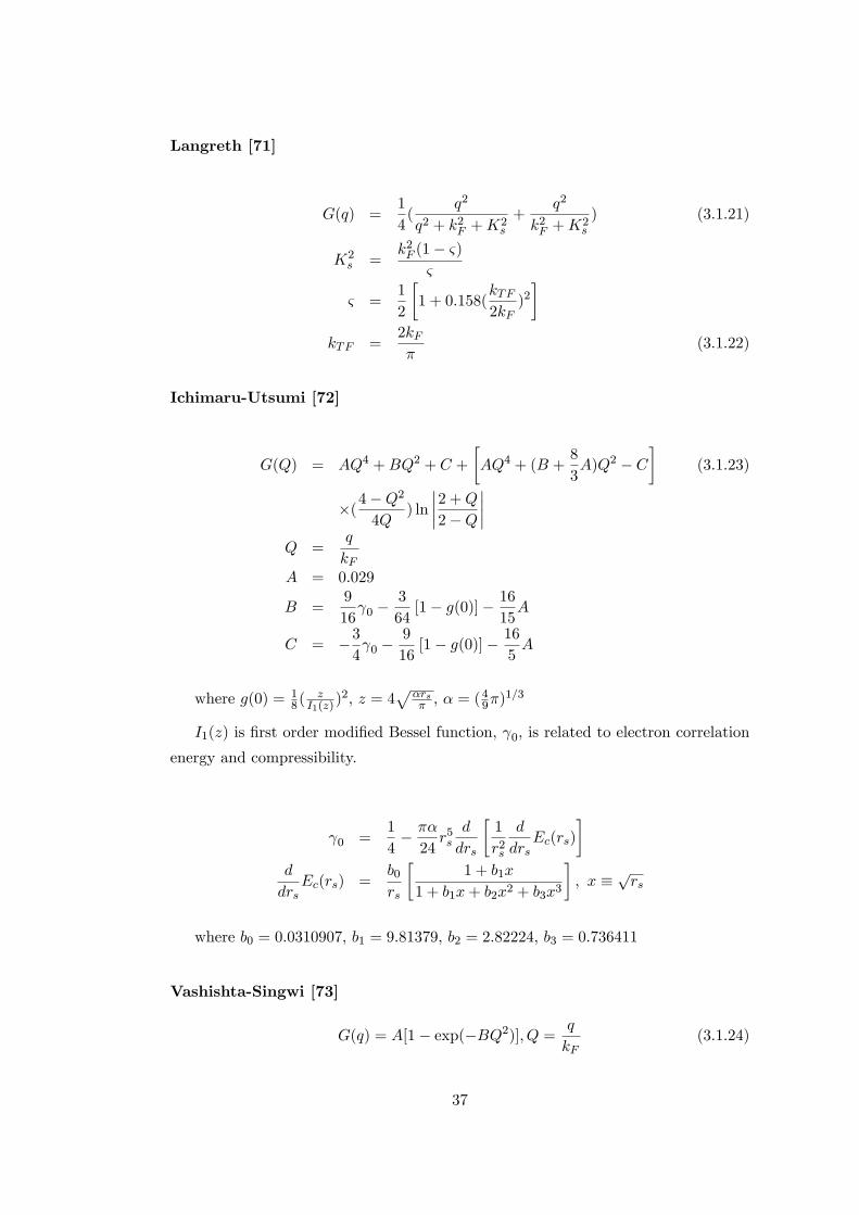
Langreth [71]

G(q) =1

4(

q2

q2 + k2F +K2s

+q2

k2F +K2s

) (3.1.21)

K2s =

k2F (1� &)&

& =1

2

�1 + 0:158(

kTF2kF

)2�

kTF =2kF�

(3.1.22)

Ichimaru-Utsumi [72]

G(Q) = AQ4 +BQ2 + C +

�AQ4 + (B +

8

3A)Q2 � C

�(3.1.23)

�(4�Q2

4Q) ln

����2 +Q2�Q

����Q =

q

kFA = 0:029

B =9

16 0 �

3

64[1� g(0)]� 16

15A

C = �34 0 �

9

16[1� g(0)]� 16

5A

where g(0) = 18(

zI1(z)

)2, z = 4p

�rs� , � = (

49�)

1=3

I1(z) is �rst order modi�ed Bessel function, 0, is related to electron correlation

energy and compressibility.

0 =1

4� ��24r5sd

drs

�1

r2s

d

drsEc(rs)

�d

drsEc(rs) =

b0rs

�1 + b1x

1 + b1x+ b2x2 + b3x3

�; x � prs

where b0 = 0:0310907, b1 = 9:81379, b2 = 2:82224, b3 = 0:736411

Vashishta-Singwi [73]

G(q) = A[1� exp(�BQ2)]; Q = q

kF(3.1.24)

37

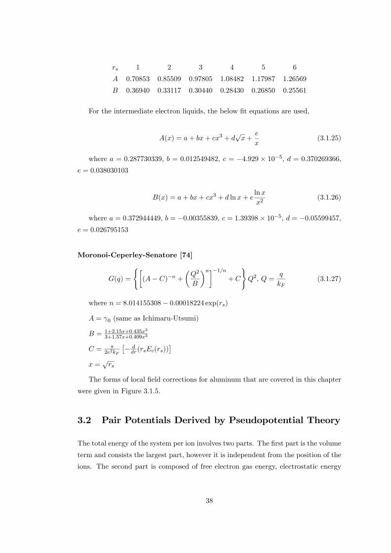
rs 1 2 3 4 5 6

A 0:70853 0:85509 0:97805 1:08482 1:17987 1:26569

B 0:36940 0:33117 0:30440 0:28430 0:26850 0:25561

For the intermediate electron liquids, the below �t equations are used,

A(x) = a+ bx+ cx3 + dpx+

e

x(3.1.25)

where a = 0:287730339, b = 0:012549482, c = �4:929 � 10�5, d = 0:370269366,

e = 0:038030103

B(x) = a+ bx+ cx3 + d lnx+ elnx

x2(3.1.26)

where a = 0:372944449, b = �0:00355839, c = 1:39398� 10�5, d = �0:05599457,e = 0:026795153

Moronoi-Ceperley-Senatore [74]

G(q) =

(�(A� C)�n +

�Q2

B

�n��1=n+ C

)Q2, Q =

q

kF(3.1.27)

where n = 8:014155308� 0:00018224 exp(rs)

A = 0 (same as Ichimaru-Utsumi)

B = 1+2:15x+0:435x3

3+1:57x+0:409x3

C = �2e2kF

�� ddr (rsEc(rs))

�x =

prs

The forms of local �eld corrections for aluminum that are covered in this chapter

were given in Figure 3.1.5.

3.2 Pair Potentials Derived by Pseudopotential Theory

The total energy of the system per ion involves two parts. The �rst part is the volume

term and consists the largest part, however it is independent from the position of the

ions. The second part is composed of free electron gas energy, electrostatic energy

38

0 1 2 3 4 50.0

0.5

1.0

1.5

2.0

2.5

3.0

3.5

4.0

G(q

)

q/kF

 Geldart­Vosko Hubbard Vashista­Singwi Moronoi Langreth Kleinmann Ichimaru­Utsumi

Figure 3.1.5: Screening functions for Aluminum.

and band energy due to ion-ion, electron-ion and electron-electron interaction. The

second order perturbation theory de�nes the band structure energy as

Ubs =Xg

jS(g)j2�bs(g) (3.2.1)

where g is the reciprocal space lattice vector, S(g) is the structure factor which

determines the ion distribution and �bs(g) is called as energy wave number charac-

teristic or characteristic function of band structure energy. The Equation 3.2.1 can

be rewritten as

Ubs =1

N2

X��

�bs(q)eiq(t��t�) (3.2.2)

In Equation 3.2.2 a sum is done over reciprocal space lattice positions and ion

types. If 'bs(r) is de�ned as the Fourier transform of �bs(q),

'bs(r) =2

(2�)3

Zd3q�bs(q)e

iqr (3.2.3)

39

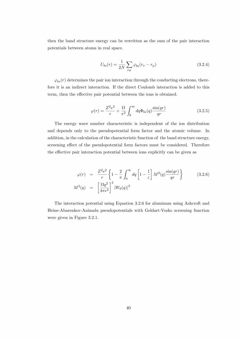
then the band structure energy can be rewritten as the sum of the pair interaction

potentials between atoms in real space.

Ubs(r) =1

2N

X��

'bs(r� � r�) (3.2.4)

'bs(r) determines the pair ion interaction through the conducting electrons, there-

fore it is an indirect interaction. If the direct Coulomb interaction is added to this

term, then the e¤ective pair potential between the ions is obtained.

'(r) =Z2e2

r+

�2

Z 1

0dq�bs(q)

sin(qr)

qr(3.2.5)

The energy wave number characteristic is independent of the ion distribution

and depends only to the pseudopotential form factor and the atomic volume. In

addition, in the calculation of the characteristic function of the band structure energy,

screening e¤ect of the pseudopotential form factors must be considered. Therefore

the e¤ective pair interaction potential between ions explicitly can be given as

'(r) =Z2e2

r

�1� 2

�

Z 1

0dq

�1� 1

"

�M2(q)

sin(qr)

qr

�(3.2.6)

M2(q) =

�q2

4�e2

�2jW0(q)j2

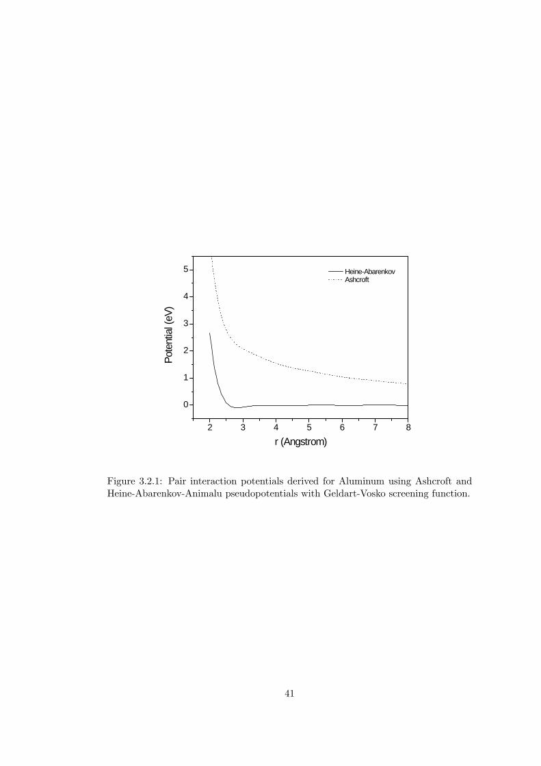
The interaction potential using Equation 3.2.6 for aluminum using Ashcroft and

Heine-Abarenkov-Animalu pseudopotentials with Geldart-Vosko screening function

were given in Figure 3.2.1.

40

2 3 4 5 6 7 8

0

1

2

3

4

5

Pote

ntia

l (eV

)

r (Angstrom)

 Heine­Abarenkov Ashcroft

Figure 3.2.1: Pair interaction potentials derived for Aluminum using Ashcroft andHeine-Abarenkov-Animalu pseudopotentials with Geldart-Vosko screening function.

41

Chapter 4

Pseudopotential based

Electromigration theory

4.1 Introduction

The electromigration theory is reviewed in aspects of thermodynamics and kinetics

by Ho and Kwok [75]. Electromigration is a basic di¤usion process under a driving

force. There is phenomenological and theoretical approaches for the determination of

this driving force in the literature [76]. It is found that the electromigration driving

force is related to the direction of motion of the electrons which is then called electron

wind force.

Electromigration driving force consists of two parts, one of which is the force

from the applied electric �eld and the other is the electron scattering force. Fiks [77]

and Huntington and Grone [78] formulated the electron wind driving force using a

ballistic approach to handle the collision of electrons with the atoms. Huntington

and Grone found that the driving force depends on the atomic con�guration of the

di¤usion path and the types of the defects. However there is a problem of seperating

the atoms, lattice and electrons in this method [14]. A quantum-mechanical model

was established by Bosvieux and Friedel [79], in which the electron scattering force

is taken as electrostatic force of the electron charge acting on the scattering center

using weak electron-ion Coulumb potentials.

Sorbello [14, 15, 16] has made a very comprehensive study about determining

the driving force for electromigration for each individual atom in a lattice with a

pseudopotential method. Sorbello reported that the electromigration force on each

42

atom consists of two di¤erent forces, one of which is the force from the applied electric

�eld and the other is the force exerted by the scattering electrons. It was reported

that the electron scattering force is caused by the impurities and vacancies in the

lattice.

In recent studies, Todorov et al [80] calculated the forces on each atom due to an

applied electric �eld by a self-consistent tight binding formalism. Dekker and Lodder

[81] has calculated the electromigration wind force in FCC and BCC metals with a

Green�s function approach.

In this study an atomistic approach to electromigration induced di¤usion in metals

is aimed to be simulated with the use of the pseudopotential method driven by

Sorbello [14], therefore a detailed discussion of this method is given in the following

section.

4.2 Pseudopotential Based Electromigration Driving Force

Sorbello [14] used a similar method with Bosvieux and Friedel [79], that is the electron

scattering force is calculated by the classical electrostatic force of the electron charge

acting on the ion. However for the electron-ion interaction, instead of weak Coulomb

potential, Sorbello suggested a pseudopotential method for the calculation of the

forces and charge densities.

Sorbello handled the force calculation in two separate parts; force on an ion arising

from the electric �eld and from the electric current which is the electron scattering

force.

Sorbello used the Born-Oppenheimer approximation to express the electron de-

pendent force on an ion j:

Fj =

Zn(r)

@V0@Rj

dr (4.2.1)

where n(r) is the electron density, V0 is the bare electron-ion interaction potential and

Rj is the ion position. Then Sorbello obtained the screened current dependent charge

density, and instead of electron-ion potential used a pseudopotential and modi�ed

Equation 4.2.1 after some derivation [14] as

Fj = �TR�@W0

@Rj(4.2.2)

43

where � is given as the current dependent part of the density operator and W0 is

the unscreened pseudopotential. After some algebra, Sorbello expressed the electron

scattering force on an ion in terms of a potential Uj :

Fj = �@Uj@Rj

(4.2.3)

where Uj is given by

Uj = �Xn

vacancies

ujn +Xi

impurities

uji (4.2.4)

and ujm is de�ned as

ujm =

8>><>>:�2mkF

4�3}2

�vdvF

�cos(vd; Rj �Rm)

R 2kF0 Wj(q)Wm(q)q

2j1(q jRj �Rmj)dq

for Rj 6= Rm�2mkF12�3}2

�vd�RjvF

� R 2kF0 Wj(q)Wm(q)q

3dq, for Rj = Rm

9>>=>>;(4.2.5)

where vd is the electron drift velocity due to applied electric �eld, vF is the Fermi

velocity, Wj(q) is the form factor of specie j, is atomic volume, j1 is the spherical

Bessel function de�ned as j1(x) = x�2 sinx� x�1 cosx.

If the above expression is applied to a perfect lattice of atoms, the contribution to

the driving force is obtained as zero. Sorbello has investigated the above expression

for di¤erent di¤usion mechanisms such as vacancy or interstitial mechanisms.

In the absence of distortion the force on a substitutional impurity, obtained by

regarding the substitutional impurity consist of an impurity and a lattice vacancy

occupying the same site, is given by

FSUB =2mkF12�3}2

�vdvF

�Z 2kF

0W2(q) [W2(q)�W1(q)] q

3dq (4.2.6)

where W2(q), and W1(q) is the form factor of substitutional impurity and host ion

respectively. In addition, the force on an atom that derives it to jump to a nearest

neighbor vacancy was given as

44

FV AC = �2mkF4�2}2

�vdvF

��2

�

Z 2kF

0W1(q)

2q2j1(q�)dq �1

3

Z 2kF

0W1(q)

2q3dq

�(4.2.7)

where � is the nearest neighbor jump distance.

45

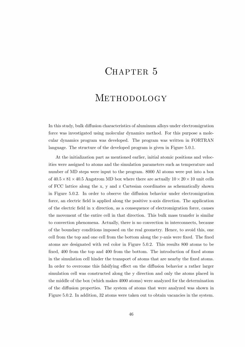
Chapter 5

Methodology

In this study, bulk di¤usion characteristics of aluminum alloys under electromigration

force was investigated using molecular dynamics method. For this purpose a mole-

cular dynamics program was developed. The program was written in FORTRAN

language. The structure of the developed program is given in Figure 5.0.1.

At the initialization part as mentioned earlier, initial atomic positions and veloc-

ities were assigned to atoms and the simulation parameters such as temperature and

number of MD steps were input to the program. 8000 Al atoms were put into a box

of 40:5� 81� 40:5 Angstrom MD box where there are actually 10� 20� 10 unit cellsof FCC lattice along the x, y and z Cartesian coordinates as schematically shown

in Figure 5.0.2. In order to observe the di¤usion behavior under electromigration

force, an electric �eld is applied along the positive x-axis direction. The application

of the electric �eld in x direction, as a consequence of electromigration force, causes

the movement of the entire cell in that direction. This bulk mass transfer is similar

to convection phenomena. Actually, there is no convection in interconnects, because

of the boundary conditions imposed on the real geometry. Hence, to avoid this, one

cell from the top and one cell from the bottom along the y-axis were �xed. The �xed

atoms are designated with red color in Figure 5.0.2. This results 800 atoms to be

�xed, 400 from the top and 400 from the bottom. The introduction of �xed atoms

in the simulation cell hinder the transport of atoms that are nearby the �xed atoms.

In order to overcome this falsifying e¤ect on the di¤usion behavior a rather larger

simulation cell was constructed along the y direction and only the atoms placed in

the middle of the box (which makes 4000 atoms) were analyzed for the determination

of the di¤usion properties. The system of atoms that were analyzed was shown in

Figure 5.0.2. In addition, 32 atoms were taken out to obtain vacancies in the system.

46

Initialization

Force Evaluation

Update positions

t>teq ?

Force evaluation

Find vacancies andcalculate

electromigration force

Update positions

Writeconfiguration

to a file

No

Yes

Equilibration

Production

t>ttot ?

Apply thermostat

Apply thermostat

No

Yes

Initial  positions  andvelocities  of  atoms  areassigned. The  controlparameters  of  thesimulation  isdetermined

The  force between  theatoms  is  calculatedusing  the  definedinteratomic potential

The  new  positions  ofthe  atoms  areobtained, using  thecalculated  forces  by  asuitable integrator.

Control  temperatureand/or pressure

Positions  of  thevacancies in the box isdetermined  and  theelectromigration  forceis calculated. Then thisforce  is  added  to  theforce obtained from theatomic interactions.

In  this  part  no  data  iscollected

All  data  is  collected  atthis part

Figure 5.0.1: Molecular dynamics program structure.

47

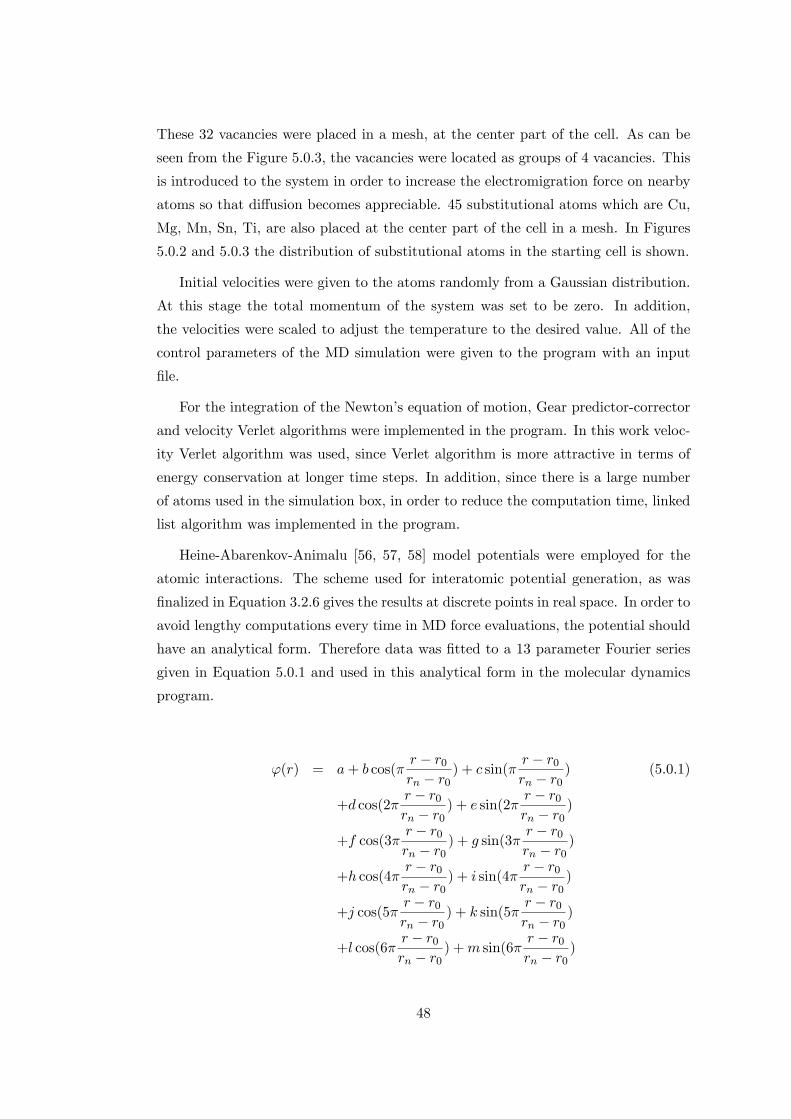
These 32 vacancies were placed in a mesh, at the center part of the cell. As can be

seen from the Figure 5.0.3, the vacancies were located as groups of 4 vacancies. This

is introduced to the system in order to increase the electromigration force on nearby

atoms so that di¤usion becomes appreciable. 45 substitutional atoms which are Cu,

Mg, Mn, Sn, Ti, are also placed at the center part of the cell in a mesh. In Figures

5.0.2 and 5.0.3 the distribution of substitutional atoms in the starting cell is shown.

Initial velocities were given to the atoms randomly from a Gaussian distribution.

At this stage the total momentum of the system was set to be zero. In addition,

the velocities were scaled to adjust the temperature to the desired value. All of the

control parameters of the MD simulation were given to the program with an input

�le.

For the integration of the Newton�s equation of motion, Gear predictor-corrector

and velocity Verlet algorithms were implemented in the program. In this work veloc-

ity Verlet algorithm was used, since Verlet algorithm is more attractive in terms of

energy conservation at longer time steps. In addition, since there is a large number

of atoms used in the simulation box, in order to reduce the computation time, linked

list algorithm was implemented in the program.

Heine-Abarenkov-Animalu [56, 57, 58] model potentials were employed for the

atomic interactions. The scheme used for interatomic potential generation, as was

�nalized in Equation 3.2.6 gives the results at discrete points in real space. In order to

avoid lengthy computations every time in MD force evaluations, the potential should

have an analytical form. Therefore data was �tted to a 13 parameter Fourier series

given in Equation 5.0.1 and used in this analytical form in the molecular dynamics

program.

'(r) = a+ b cos(�r � r0rn � r0

) + c sin(�r � r0rn � r0

) (5.0.1)

+d cos(2�r � r0rn � r0

) + e sin(2�r � r0rn � r0

)

+f cos(3�r � r0rn � r0

) + g sin(3�r � r0rn � r0

)

+h cos(4�r � r0rn � r0

) + i sin(4�r � r0rn � r0

)

+j cos(5�r � r0rn � r0

) + k sin(5�r � r0rn � r0

)

+l cos(6�r � r0rn � r0

) +m sin(6�r � r0rn � r0

)

48

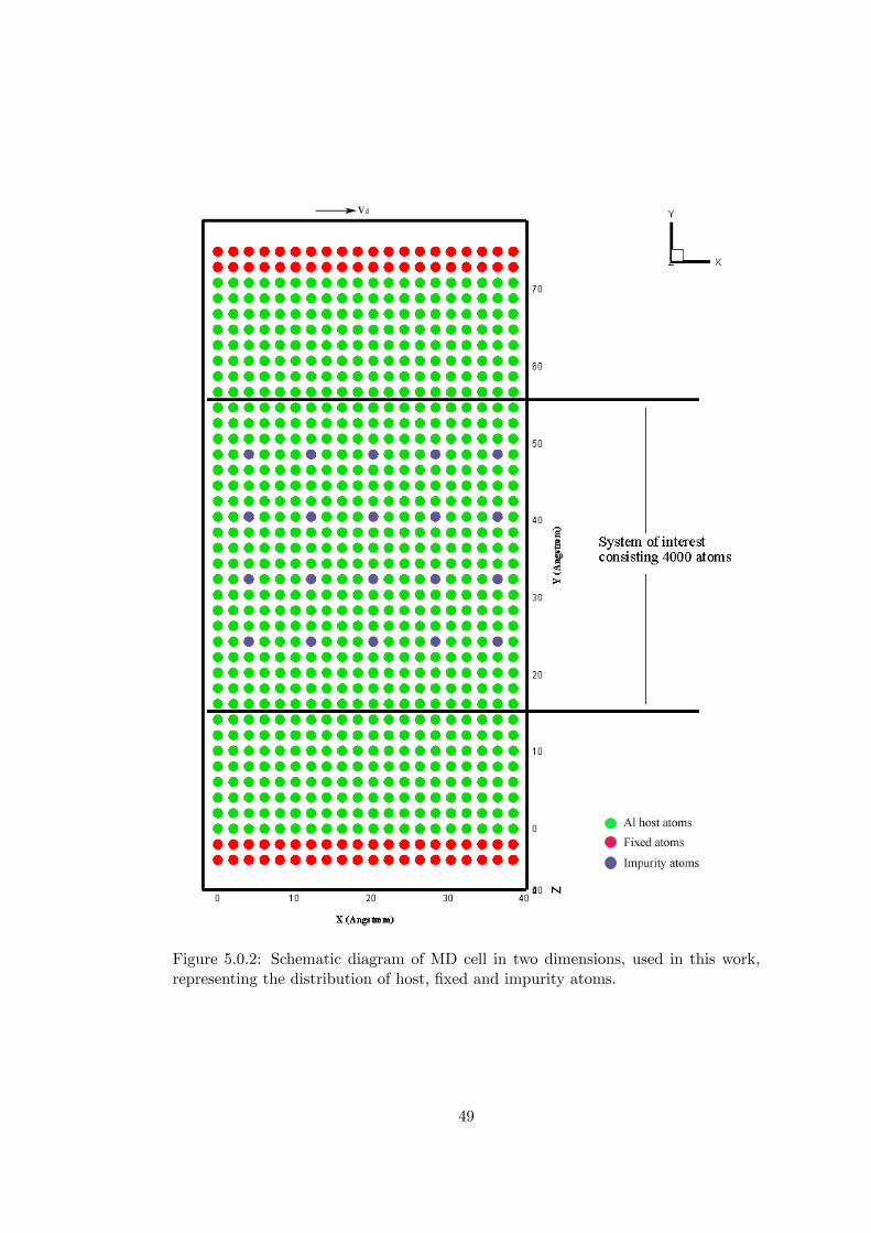
Figure 5.0.2: Schematic diagram of MD cell in two dimensions, used in this work,representing the distribution of host, �xed and impurity atoms.

49

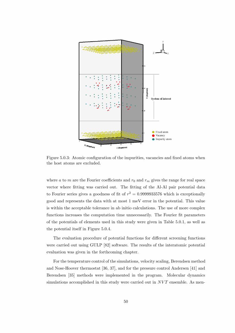
Figure 5.0.3: Atomic con�guration of the impurities, vacancies and �xed atoms whenthe host atoms are excluded.

where a to m are the Fourier coe¢ cients and r0 and rm gives the range for real space

vector where �tting was carried out. The �tting of the Al-Al pair potential data

to Fourier series gives a goodness of �t of r2 = 0:9999933576 which is exceptionally

good and represents the data with at most 1 meV error in the potential. This value

is within the acceptable tolerance in ab initio calculations. The use of more complex

functions increases the computation time unnecessarily. The Fourier �t parameters

of the potentials of elements used in this study were given in Table 5.0.1, as well as

the potential itself in Figure 5.0.4.

The evaluation procedure of potential functions for di¤erent screening functions

were carried out using GULP [82] software. The results of the interatomic potential

evaluation was given in the forthcoming chapter.

For the temperature control of the simulations, velocity scaling, Berendsen method

and Nose-Hoover thermostat [36, 37], and for the pressure control Andersen [41] and

Berendsen [35] methods were implemented in the program. Molecular dynamics

simulations accomplished in this study were carried out in NV T ensemble. As men-

50

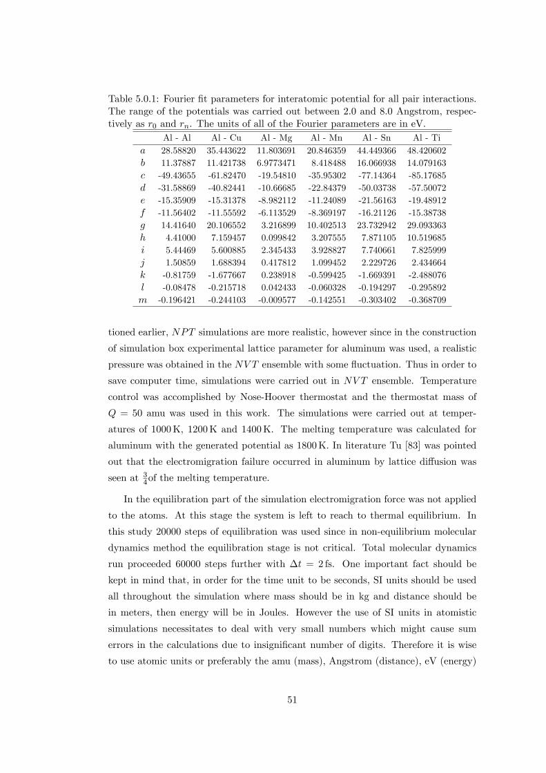
Table 5.0.1: Fourier �t parameters for interatomic potential for all pair interactions.The range of the potentials was carried out between 2.0 and 8.0 Angstrom, respec-tively as r0 and rn. The units of all of the Fourier parameters are in eV.

Al - Al Al - Cu Al - Mg Al - Mn Al - Sn Al - Tia 28.58820 35.443622 11.803691 20.846359 44.449366 48.420602b 11.37887 11.421738 6.9773471 8.418488 16.066938 14.079163c -49.43655 -61.82470 -19.54810 -35.95302 -77.14364 -85.17685d -31.58869 -40.82441 -10.66685 -22.84379 -50.03738 -57.50072e -15.35909 -15.31378 -8.982112 -11.24089 -21.56163 -19.48912f -11.56402 -11.55592 -6.113529 -8.369197 -16.21126 -15.38738g 14.41640 20.106552 3.216899 10.402513 23.732942 29.093363h 4.41000 7.159457 0.099842 3.207555 7.871105 10.519685i 5.44469 5.600885 2.345433 3.928827 7.740661 7.825999j 1.50859 1.688394 0.417812 1.099452 2.229726 2.434664k -0.81759 -1.677667 0.238918 -0.599425 -1.669391 -2.488076l -0.08478 -0.215718 0.042433 -0.060328 -0.194297 -0.295892m -0.196421 -0.244103 -0.009577 -0.142551 -0.303402 -0.368709

tioned earlier, NPT simulations are more realistic, however since in the construction

of simulation box experimental lattice parameter for aluminum was used, a realistic

pressure was obtained in the NV T ensemble with some �uctuation. Thus in order to

save computer time, simulations were carried out in NV T ensemble. Temperature

control was accomplished by Nose-Hoover thermostat and the thermostat mass of

Q = 50 amu was used in this work. The simulations were carried out at temper-

atures of 1000K, 1200K and 1400K. The melting temperature was calculated for

aluminum with the generated potential as 1800K: In literature Tu [83] was pointed

out that the electromigration failure occurred in aluminum by lattice di¤usion was

seen at 34of the melting temperature.

In the equilibration part of the simulation electromigration force was not applied

to the atoms. At this stage the system is left to reach to thermal equilibrium. In

this study 20000 steps of equilibration was used since in non-equilibrium molecular

dynamics method the equilibration stage is not critical. Total molecular dynamics

run proceeded 60000 steps further with �t = 2 fs. One important fact should be

kept in mind that, in order for the time unit to be seconds, SI units should be used

all throughout the simulation where mass should be in kg and distance should be

in meters; then energy will be in Joules. However the use of SI units in atomistic

simulations necessitates to deal with very small numbers which might cause sum

errors in the calculations due to insigni�cant number of digits. Therefore it is wise

to use atomic units or preferably the amu (mass), Angstrom (distance), eV (energy)

51

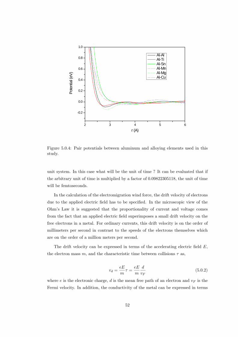
2 3 4 5 6

­0.2

0.0

0.2

0.4

0.6

0.8

1.0

Pote

ntia

l (eV

)

r (A)

Al­AlAl­TiAl­SnAl­MnAl­MgAl­Cu

Figure 5.0.4: Pair potentials between aluminum and alloying elements used in thisstudy.

unit system. In this case what will be the unit of time ? It can be evaluated that if

the arbitrary unit of time is multiplied by a factor of 0:09822305118, the unit of time

will be femtoseconds.

In the calculation of the electromigration wind force, the drift velocity of electrons

due to the applied electric �eld has to be speci�ed. In the microscopic view of the

Ohm�s Law it is suggested that the proportionality of current and voltage comes

from the fact that an applied electric �eld superimposes a small drift velocity on the

free electrons in a metal. For ordinary currents, this drift velocity is on the order of

millimeters per second in contrast to the speeds of the electrons themselves which

are on the order of a million meters per second.

The drift velocity can be expressed in terms of the accelerating electric �eld E,

the electron mass m, and the characteristic time between collisions � as,

vd =eE

m� =

eE

m

d

vF(5.0.2)

where e is the electronic charge, d is the mean free path of an electron and vF is the

Fermi velocity. In addition, the conductivity of the metal can be expressed in terms

52

of the density of the free electrons, n, as

� =ne2d

mvF(5.0.3)

Combining Equations 5.0.2, 5.0.3 and the Ohm�s Law, J = �E, where J is the

electric current density, we have

vd =�E

ne=J

ne(5.0.4)

Since the stable oxidation state of Al is three, the number of free electrons per

m3 of Al will be, n = 3NA�A = 1:815� 1029 electrons/m3 where NA is the Avogadro�snumber, � is the density and A is the atomic weight. Assuming that, under normal

operating conditions of integrated devices, current density can be as high as 1010

A/m2 then, the drift velocity for Al will be calculated as 0:34 m/s. Conversion from

SI units to atomic units gives the drift velocity as 1:5 � 10�7 a.u. In this study wehave used 0:01 a.u. drift velocity. Although it is a rather high value compared to

experiment, it was necessary to use such high values in order to observe an appreciable

di¤usion in a quite limited amount of real simulation time which is only 0:12 ps, where

the simulation was carried out at almost half of the melting temperature.

The electromigration force was calculated by the use of a pseudopotential ap-

proach of Sorbello [14], where in this approach Heine-Abarenkov-Animalu form fac-

tors are used. The calculated electromigration force was added to the force obtained

from the interatomic interactions at the corrector stage of the integration part. This

added force can be thought as a perturbation which causes non-equilibrium conditions

to be imposed on the system.

As mentioned earlier the electromigration force on atom j due to an applied elec-

tric �eld depends on the impurities and vacancies in the lattice, given by Equations

4.2.3 and 4.2.4.

Fj = �@Uj@Rj

Uj = �Xn

vacancies

ujn +Xi

impurities

uji

where ujm has to be de�ned for all of the possible cases of pair interactions. The

53

possible pairs and their contribution to the potential in the calculation of electromi-

gration force on the jth atom is given in the Table 5.0.2.

In addition, the force distribution near a vacancy in an aluminum lattice and

the electromigration force on various subtitutional atoms in an aluminum lattice was

calculated separately from molecular dynamics simulations, actually before going

into detailed MD studies. The aim was to determine the candidate substitutionals in

aluminum that would have smaller electromigration force on them.

The evaluation of the force on the atoms due to neighbouring vacancies in the

lattice is not an easy process compared to the force calculation due to the impurities

in the lattice, since during the simulation, the positions of the vacancies should be

traced. To determine the positions of the vacancies in each MD step, a subprogram

was developed and this routine was called before each electromigration force calcu-

lation. The routine works in such a manner that the vacancies can be only located

at perfect lattice sites. For each perfect lattice position therefore a sphere was con-

structed and it is controlled if there is any nearby atom located in this sphere. All

of the atomic positions and their image positions in the MD cell is controlled for one

perfect lattice position. The radius of the sphere is determined by several trials that

give the correct vacancy number, which is introduced at the initialization part of the

program. 1.145 Å of radius is used in this study compared to 1.431Å of half of the

nearest neighbor distance in FCC aluminum.

In order to investigate the di¤usion behavior of a material by molecular dynamics

method, di¤usion coe¢ cient can be calculated by mean square displacement (MSD)

(see Equation 2.1.34) or by velocity autocorrelation function (VAF) (see Equation

2.1.36). In non-equilibrium molecular dynamics however, Equation 2.2.11 can be

used. In this study there is an applied electric �eld on the system, and this causes

an electromigration force exerted on the atoms. This imposes the non-equilibrium

conditions, thus excludes the use of MSD or VAF, since in non-equilibrium systems,

approaches of statistical mechanics could not be used. Moreover, the treatment in

NEMD can not di¤erentiate the atomic species.

The calculation of the di¤usion coe¢ cient via EMD or NEMD approaches seems

not to be possible under the conditions of the simulation in this study. In that case

nothing but the basic de�nition of atomic transport is left, which is atomic jump

frequency and it is de�ned as

54

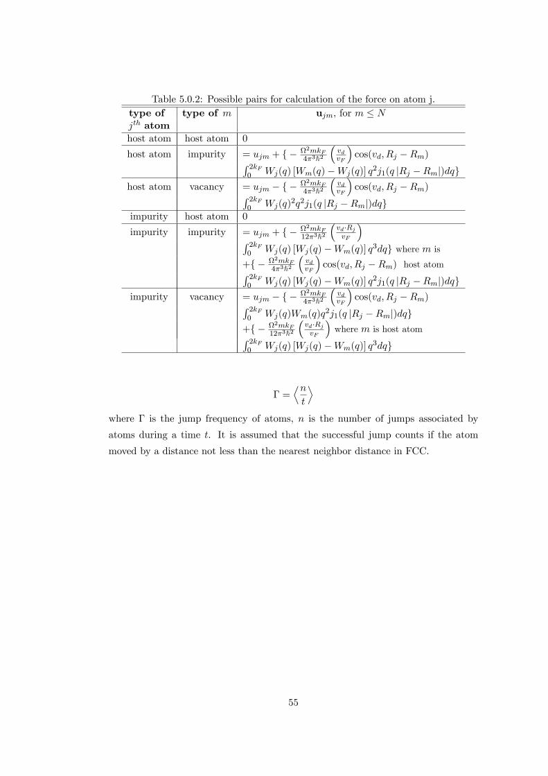
Table 5.0.2: Possible pairs for calculation of the force on atom j.type of type of m ujm, for m � Njth atomhost atom host atom 0

host atom impurity = ujm + f � 2mkF4�3}2

�vdvF

�cos(vd; Rj �Rm)R 2kF

0 Wj(q) [Wm(q)�Wj(q)] q2j1(q jRj �Rmj)dqg

host atom vacancy = ujm � f � 2mkF4�3}2

�vdvF

�cos(vd; Rj �Rm)R 2kF

0 Wj(q)2q2j1(q jRj �Rmj)dqg

impurity host atom 0

impurity impurity = ujm + f � 2mkF12�3}2

�vd�RjvF

�R 2kF0 Wj(q) [Wj(q)�Wm(q)] q

3dqg where m is

+f � 2mkF4�3}2

�vdvF

�cos(vd; Rj �Rm) host atomR 2kF

0 Wj(q) [Wj(q)�Wm(q)] q2j1(q jRj �Rmj)dqg

impurity vacancy = ujm � f � 2mkF4�3}2

�vdvF

�cos(vd; Rj �Rm)R 2kF

0 Wj(q)Wm(q)q2j1(q jRj �Rmj)dqg

+f � 2mkF12�3}2

�vd�RjvF

�where m is host atomR 2kF

0 Wj(q) [Wj(q)�Wm(q)] q3dqg

� =Dnt

Ewhere � is the jump frequency of atoms, n is the number of jumps associated by

atoms during a time t. It is assumed that the successful jump counts if the atom

moved by a distance not less than the nearest neighbor distance in FCC.

55

Chapter 6

Results and Discussion

6.1 Critical Potential Evaluation for Aluminum

For the evaluation of atomic interactions in the molecular dynamics simulations, pair

potentials were constructed using Heine-Abarenkov-Animalu model pseudopotentials.

Various screening functions, which are Hubbard, Kleinman, Langreth, Geldart-Vosko,

Ichimaru-Utsumi, Moronoi and Vashishta-Singwi screening functions, were used in

the potential production for aluminum. The obtained potentials were given in Figure

6.1.1.

The potentials used in the simulations should be tested in order to be con�dent

about their applicability in simulations. For this purpose the validity of the poten-

tials produced with di¤erent screening functions were tested by GULP [82] software

and some of the properties, which were lattice parameter, lattice energy and elastic

constants of aluminum were calculated and compared with the experimental ones,

as given in Table 6.1.1. First and one of the most important expectation from the

potential is its capability to predict the right ground state, which is FCC for Al. As

can be seen from Table 6.1.1 for all screening functions and from Figure 6.1.2 in detail

for Geldart-Vosko screening, the right ground state FCC was predicted. Then the

analysis of the lattice parameter, elastic constants, etc. becomes important. The best

prediction of the lattice parameter was obtained with Geldart-Vosko screening, see

Table 6.1.1. It predicts the lattice parameter with 2.96% error. Therefore, Geldart-

Vosko was chosen as the screening function for the production model pair potentials

using Heine-Abarenkov-Animalu pseudopotential form factors.

56

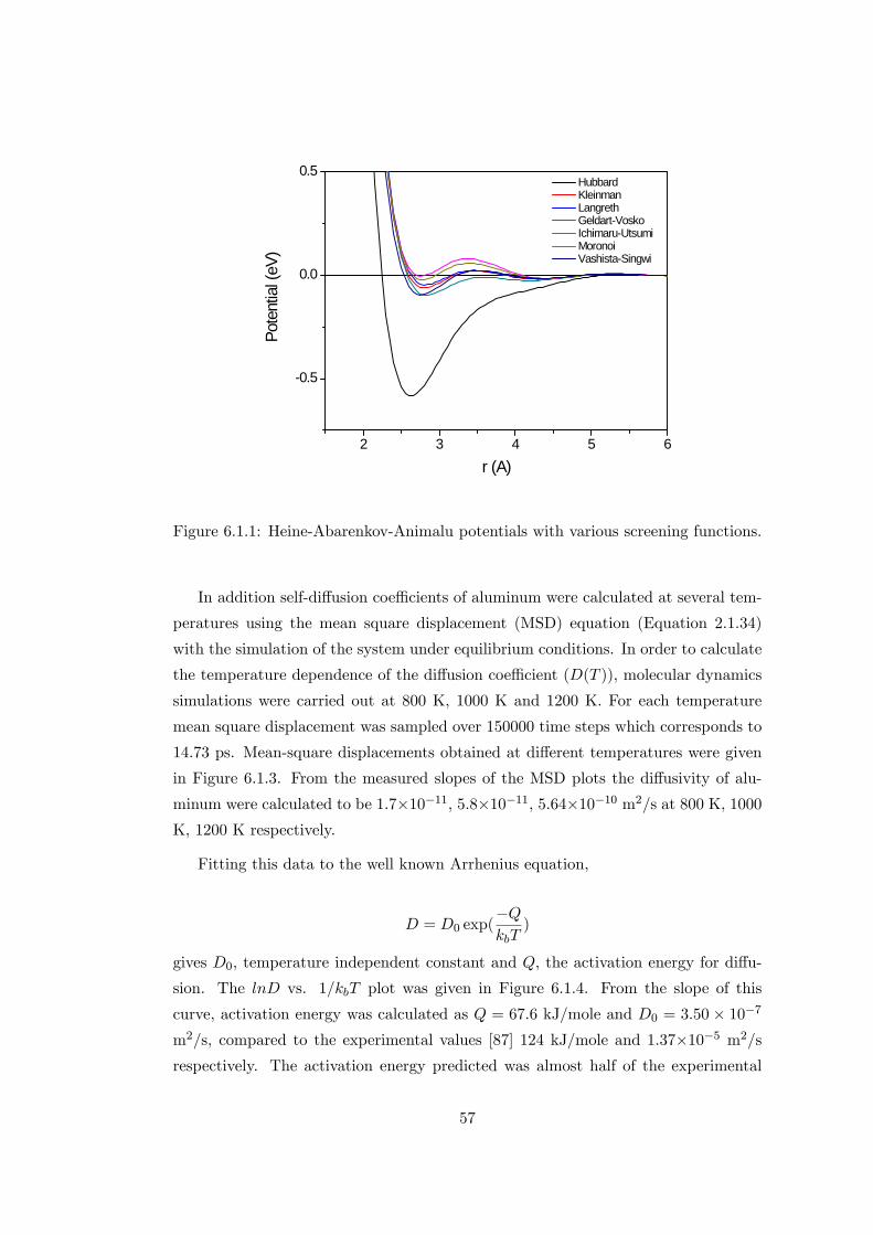
2 3 4 5 6

­0.5

0.0

0.5

Pote

ntia

l (eV

)

r (A)

HubbardKleinmanLangrethGeldart­VoskoIchimaru­UtsumiMoronoiVashista­Singwi

Figure 6.1.1: Heine-Abarenkov-Animalu potentials with various screening functions.

In addition self-di¤usion coe¢ cients of aluminum were calculated at several tem-

peratures using the mean square displacement (MSD) equation (Equation 2.1.34)

with the simulation of the system under equilibrium conditions. In order to calculate

the temperature dependence of the di¤usion coe¢ cient (D(T )), molecular dynamics

simulations were carried out at 800 K, 1000 K and 1200 K. For each temperature

mean square displacement was sampled over 150000 time steps which corresponds to

14.73 ps. Mean-square displacements obtained at di¤erent temperatures were given

in Figure 6.1.3. From the measured slopes of the MSD plots the di¤usivity of alu-

minum were calculated to be 1.7�10�11, 5.8�10�11, 5.64�10�10 m2/s at 800 K, 1000K, 1200 K respectively.

Fitting this data to the well known Arrhenius equation,

D = D0 exp(�QkbT

)

gives D0; temperature independent constant and Q; the activation energy for di¤u-

sion. The lnD vs. 1=kbT plot was given in Figure 6.1.4. From the slope of this

curve, activation energy was calculated as Q = 67:6 kJ/mole and D0 = 3:50 � 10�7

m2/s, compared to the experimental values [87] 124 kJ/mole and 1.37�10�5 m2=srespectively. The activation energy predicted was almost half of the experimental

57

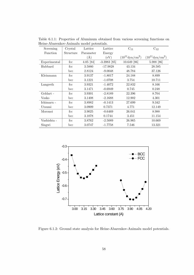
Table 6.1.1: Properties of Aluminum obtained from various screening functions onHeine-Abarenkov-Animalu model potentials.

Screening Crystal Lattice Lattice C11 C12Function Structure Parameter Energy

(Å) (eV) (1011dyn/cm2) (1011dyn/cm2)Experimental fcc 4.05 [84] -3.3983 [85] 10.649 [86] 5.988 [86]Hubbard fcc 3.5880 -17.9828 43.134 28.585

bcc 2.8124 -9.0048 48.784 37.126Kleinmann fcc 3.9137 -1.8017 24.188 8.899

bcc 3.1221 -1.0708 3.754 10.711Langreth fcc 3.9321 -1.4072 22.832 8.166

bcc 3.1471 -0.6949 0.745 0.248Geldart - fcc 3.9301 -2.8189 22.396 8.704Vosko bcc 3.1408 -2.1688 12.902 4.301Ichimaru - fcc 3.8982 -0.1413 27.699 9.342Utsumi bcc 3.0909 0.7371 4.771 12.149Moronoi fcc 3.9025 -0.6469 26.041 8.988

bcc 3.1078 0.1744 3.451 11.154Vashishta - fcc 3.8762 -2.5089 26.965 10.669Singwi bcc 3.0747 -1.7758 7.546 13.321

3.00 3.15 3.30 3.45 3.60 3.75 3.90 4.05 4.20

­0.7

­0.6

­0.5

­0.4

­0.3

Latti

ce E

nerg

y (e

V)

Lattice constant (A)

BCCFCC

Figure 6.1.2: Ground state analysis for Heine-Abarenkov-Animalu model potentials.

58

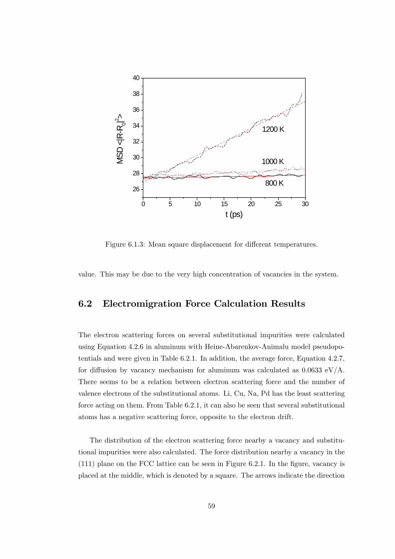
0 5 10 15 20 25 30

26

28

30

32

34

36

38

40

MSD

 <|R

­R0|2 >

t (ps)

1200 K

1000 K

800 K

Figure 6.1.3: Mean square displacement for di¤erent temperatures.

value. This may be due to the very high concentration of vacancies in the system.

6.2 Electromigration Force Calculation Results

The electron scattering forces on several substitutional impurities were calculated

using Equation 4.2.6 in aluminum with Heine-Abarenkov-Animalu model pseudopo-

tentials and were given in Table 6.2.1. In addition, the average force, Equation 4.2.7,

for di¤usion by vacancy mechanism for aluminum was calculated as 0.0633 eV/A.

There seems to be a relation between electron scattering force and the number of

valence electrons of the substitutional atoms. Li, Cu, Na, Pd has the least scattering

force acting on them. From Table 6.2.1, it can also be seen that several substitutional

atoms has a negative scattering force, opposite to the electron drift.

The distribution of the electron scattering force nearby a vacancy and substitu-

tional impurities were also calculated. The force distribution nearby a vacancy in the

(111) plane on the FCC lattice can be seen in Figure 6.2.1. In the �gure, vacancy is

placed at the middle, which is denoted by a square. The arrows indicate the direction

59

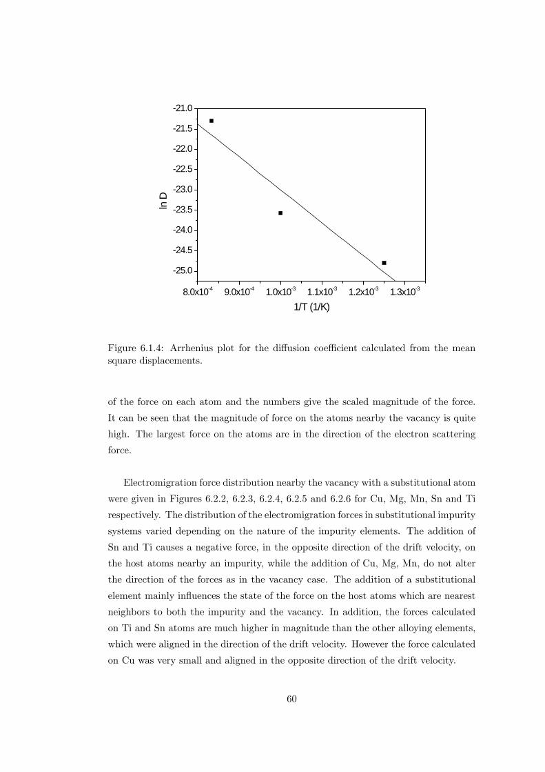
8.0x10­4 9.0x10­4 1.0x10­3 1.1x10­3 1.2x10­3 1.3x10­3

­25.0

­24.5

­24.0

­23.5

­23.0

­22.5

­22.0

­21.5

­21.0

ln D

1/T (1/K)

Figure 6.1.4: Arrhenius plot for the di¤usion coe¢ cient calculated from the meansquare displacements.

of the force on each atom and the numbers give the scaled magnitude of the force.

It can be seen that the magnitude of force on the atoms nearby the vacancy is quite

high. The largest force on the atoms are in the direction of the electron scattering

force.

Electromigration force distribution nearby the vacancy with a substitutional atom

were given in Figures 6.2.2, 6.2.3, 6.2.4, 6.2.5 and 6.2.6 for Cu, Mg, Mn, Sn and Ti

respectively. The distribution of the electromigration forces in substitutional impurity

systems varied depending on the nature of the impurity elements. The addition of

Sn and Ti causes a negative force, in the opposite direction of the drift velocity, on

the host atoms nearby an impurity, while the addition of Cu, Mg, Mn, do not alter

the direction of the forces as in the vacancy case. The addition of a substitutional

element mainly in�uences the state of the force on the host atoms which are nearest

neighbors to both the impurity and the vacancy. In addition, the forces calculated

on Ti and Sn atoms are much higher in magnitude than the other alloying elements,

which were aligned in the direction of the drift velocity. However the force calculated

on Cu was very small and aligned in the opposite direction of the drift velocity.

60

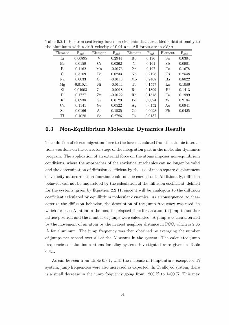
Table 6.2.1: Electron scattering forces on elements that are added subtitutionally tothe aluminum with a drift velocity of 0.01 a.u. All forces are in eV/A.

Element Fsub Element Fsub Element Fsub Element FsubLi 0.00895 V 0.2944 Rb 0.196 Sn 0.0304Be 0.0159 Cr 0.0362 Y 0.161 Sb 0.0901B 0.1162 Mn -0.0173 Zr 0.197 Te 0.1678C 0.3169 Fe 0.0233 Nb 0.2128 Cs 0.2548Na 0.0033 Co -0.0143 Mo 0.2468 Ba 0.8022Mg -0.01024 Ni -0.0144 Tc 0.1557 La 0.1086Si 0.04903 Cu -0.0018 Ru 0.1899 Hf 0.1413P 0.1727 Zn -0.0122 Rh 0.1518 Ta 0.1999K 0.0938 Ga 0.0123 Pd 0.0024 W 0.2184Ca 0.1141 Ge 0.0522 Ag 0.0152 Au 0.0941Sc 0.0166 As 0.1535 Cd 0.0098 Pb 0.0425Ti 0.1028 Se 0.2786 In 0.0137

6.3 Non-Equilibrium Molecular Dynamics Results

The addition of electromigration force to the force calculated from the atomic interac-

tions was done on the corrector stage of the integration part in the molecular dynamics

program. The application of an external force on the atoms imposes non-equilibrium

conditions, where the approaches of the statistical mechanics can no longer be valid

and the determination of di¤usion coe¢ cient by the use of mean square displacement

or velocity autocorrelation function could not be carried out. Additionally, di¤usion

behavior can not be understood by the calculation of the di¤usion coe¢ cient, de�ned

for the systems, given by Equation 2.2.11, since it will be analogous to the di¤usion

coe¢ cient calculated by equilibrium molecular dynamics. As a consequence, to char-

acterize the di¤usion behavior, the description of the jump frequency was used, in

which for each Al atom in the box, the elapsed time for an atom to jump to another

lattice position and the number of jumps were calculated. A jump was characterized

by the movement of an atom by the nearest neighbor distance in FCC, which is 2.86

Å for aluminum. The jump frequency was then obtained by averaging the number

of jumps per second over all of the Al atoms in the system. The calculated jump

frequencies of aluminum atoms for alloy systems investigated were given in Table

6.3.1.

As can be seen from Table 6.3.1, with the increase in temperature, except for Ti

system, jump frequencies were also increased as expected. In Ti alloyed system, there

is a small decrease in the jump frequency going from 1200 K to 1400 K. This may

61

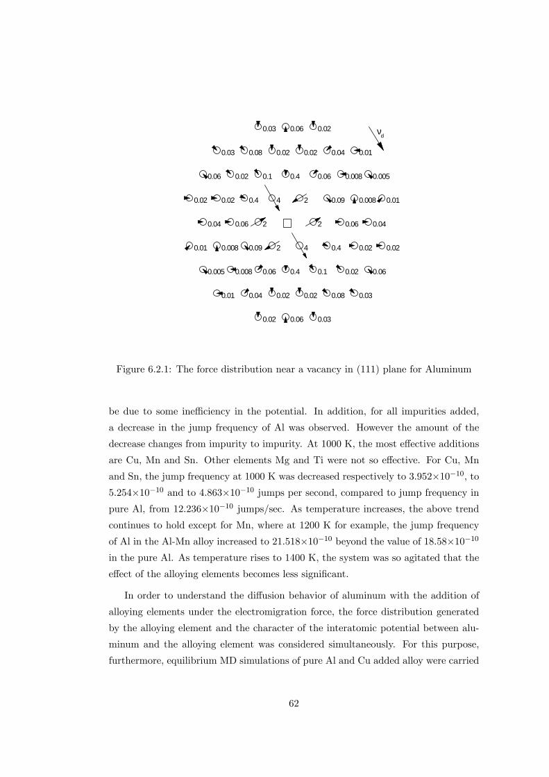
0.01 0.04 0.02

0.06

0.02

0.02

0.08 0.03

0.03

0.01

0.005

0.008 0.09

0.06

2

0.008

4

0.1

0.4

0.4

0.02

0.06

0.02

0.02

0.02 0.02

0.06

0.4

0.04

4 2

2

0.09

0.06

0.008

2

0.01

0.04

0.06

0.03 0.08

0.1

0.02

0.02

0.02

0.06

0.04

0.4

0.01

0.0050.008

0.060.03 0.02 νd

Figure 6.2.1: The force distribution near a vacancy in (111) plane for Aluminum

be due to some ine¢ ciency in the potential. In addition, for all impurities added,

a decrease in the jump frequency of Al was observed. However the amount of the

decrease changes from impurity to impurity. At 1000 K, the most e¤ective additions

are Cu, Mn and Sn. Other elements Mg and Ti were not so e¤ective. For Cu, Mn

and Sn, the jump frequency at 1000 K was decreased respectively to 3.952�10�10, to5.254�10�10 and to 4.863�10�10 jumps per second, compared to jump frequency inpure Al, from 12.236�10�10 jumps/sec. As temperature increases, the above trendcontinues to hold except for Mn, where at 1200 K for example, the jump frequency

of Al in the Al-Mn alloy increased to 21.518�10�10 beyond the value of 18.58�10�10

in the pure Al. As temperature rises to 1400 K, the system was so agitated that the

e¤ect of the alloying elements becomes less signi�cant.

In order to understand the di¤usion behavior of aluminum with the addition of

alloying elements under the electromigration force, the force distribution generated

by the alloying element and the character of the interatomic potential between alu-

minum and the alloying element was considered simultaneously. For this purpose,

furthermore, equilibrium MD simulations of pure Al and Cu added alloy were carried

62

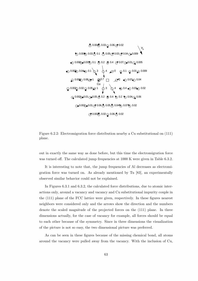
0.7

0.002 0.01

0.003

0.06 0.05

0.06

0.04

0.02

0.07 0.02

0.02

0.002 0.02

0.01

0.05

0.003

1

0.2

3

0.05

4

0.2

0.4

0.4

0.03

0.06

0.02

0.04

0.003

0.006

0.04 0.1

1

3

0.08

4 2 0.1

0.07

0.01

2

0.009

0.04

0.004

0.03

0.03

0.008

0.1

0.2

0.05

0.1

0.03

0.07

0.04

0.4

0.009

0.0050.01

0.004 0.060.03 0.02νd

Cu

Figure 6.2.2: Electromigration force distribution nearby a Cu substitutional on (111)plane.

out in exactly the same way as done before, but this time the electromigration force

was turned o¤. The calculated jump frequencies at 1000 K were given in Table 6.3.2.

It is interesting to note that, the jump frequencies of Al decreases as electromi-

gration force was turned on. As already mentioned by Tu [83], an experimentally

observed similar behavior could not be explained.

In Figures 6.3.1 and 6.3.2, the calculated force distributions, due to atomic inter-

actions only, around a vacancy and vacancy and Cu substitutional impurity couple in

the (111) plane of the FCC lattice were given, respectively. In these �gures nearest

neighbors were considered only and the arrows show the direction and the numbers

denote the scaled magnitude of the projected forces on the (111) plane. In three

dimensions actually, for the case of vacancy for example, all forces should be equal

to each other because of the symmetry. Since in three dimensions the visualization

of the picture is not so easy, the two dimensional picture was preferred.

As can be seen in these �gures because of the missing chemical bond, all atoms

around the vacancy were pulled away from the vacancy. With the inclusion of Cu,

63

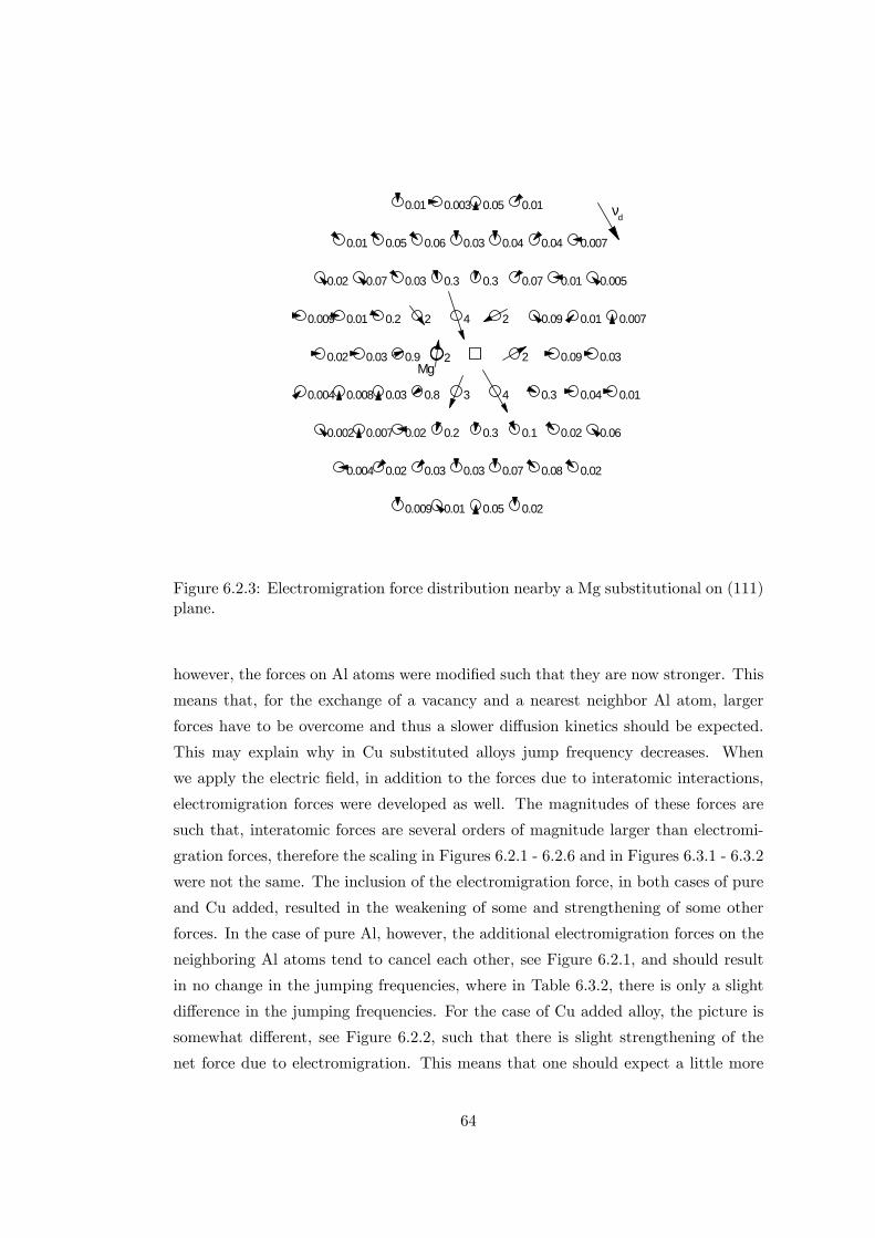
0.004 0.02

0.009

0.03 0.03

0.05

0.07

0.01

0.08 0.02

0.02

0.004 0.008

0.007

0.03

0.002

0.8

0.2

3

0.02

4

0.1

0.3

0.3

0.04

0.06

0.01

0.02

0.009

0.02

0.01 0.2

0.9

2

0.03

4 2 0.09

0.09

0.01

2

0.007

0.03

0.01

0.07

0.05

0.02

0.06

0.3

0.03

0.03

0.04

0.07

0.04

0.3

0.007

0.0050.01

0.01 0.050.003 0.01

2Mg

νd

Figure 6.2.3: Electromigration force distribution nearby a Mg substitutional on (111)plane.

however, the forces on Al atoms were modi�ed such that they are now stronger. This

means that, for the exchange of a vacancy and a nearest neighbor Al atom, larger

forces have to be overcome and thus a slower di¤usion kinetics should be expected.

This may explain why in Cu substituted alloys jump frequency decreases. When

we apply the electric �eld, in addition to the forces due to interatomic interactions,

electromigration forces were developed as well. The magnitudes of these forces are

such that, interatomic forces are several orders of magnitude larger than electromi-

gration forces, therefore the scaling in Figures 6.2.1 - 6.2.6 and in Figures 6.3.1 - 6.3.2

were not the same. The inclusion of the electromigration force, in both cases of pure

and Cu added, resulted in the weakening of some and strengthening of some other

forces. In the case of pure Al, however, the additional electromigration forces on the

neighboring Al atoms tend to cancel each other, see Figure 6.2.1, and should result

in no change in the jumping frequencies, where in Table 6.3.2, there is only a slight

di¤erence in the jumping frequencies. For the case of Cu added alloy, the picture is

somewhat di¤erent, see Figure 6.2.2, such that there is slight strengthening of the

net force due to electromigration. This means that one should expect a little more

64

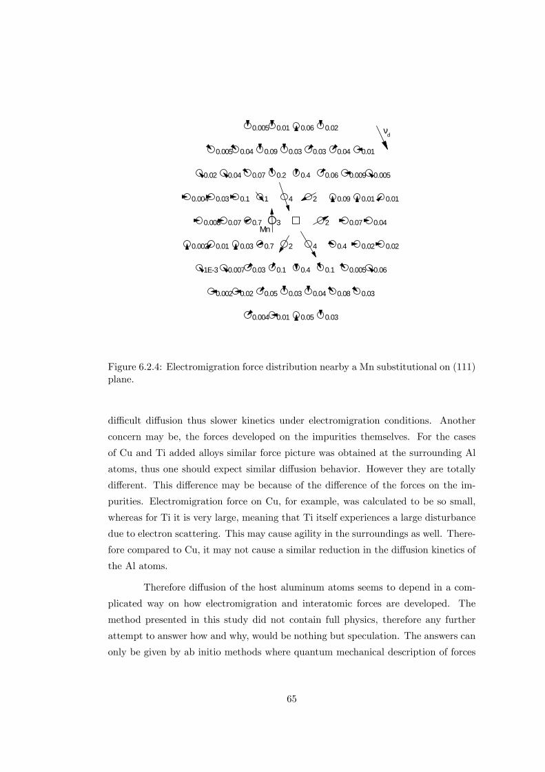
0.002 0.02

0.004

0.05 0.03

0.05

0.04

0.01

0.08 0.03

0.03

0.002 0.01

0.007

0.03

1E­3

0.7

0.1

2

0.03

4

0.1

0.4

0.4

0.02

0.06

0.02

0.005

0.004

0.008

0.03 0.1

0.7

1

0.07

4 2 0.09

0.07

0.01

2

0.01

0.04

0.005

0.04

0.04

0.02

0.09

0.2

0.03

0.07

0.03

0.06

0.04

0.4

0.01

0.0050.009

0.005 0.060.01 0.02

3Mn

νd

Figure 6.2.4: Electromigration force distribution nearby a Mn substitutional on (111)plane.

di¢ cult di¤usion thus slower kinetics under electromigration conditions. Another

concern may be, the forces developed on the impurities themselves. For the cases

of Cu and Ti added alloys similar force picture was obtained at the surrounding Al

atoms, thus one should expect similar di¤usion behavior. However they are totally

di¤erent. This di¤erence may be because of the di¤erence of the forces on the im-

purities. Electromigration force on Cu, for example, was calculated to be so small,

whereas for Ti it is very large, meaning that Ti itself experiences a large disturbance

due to electron scattering. This may cause agility in the surroundings as well. There-

fore compared to Cu, it may not cause a similar reduction in the di¤usion kinetics of

the Al atoms.

Therefore di¤usion of the host aluminum atoms seems to depend in a com-

plicated way on how electromigration and interatomic forces are developed. The

method presented in this study did not contain full physics, therefore any further

attempt to answer how and why, would be nothing but speculation. The answers can

only be given by ab initio methods where quantum mechanical description of forces

65

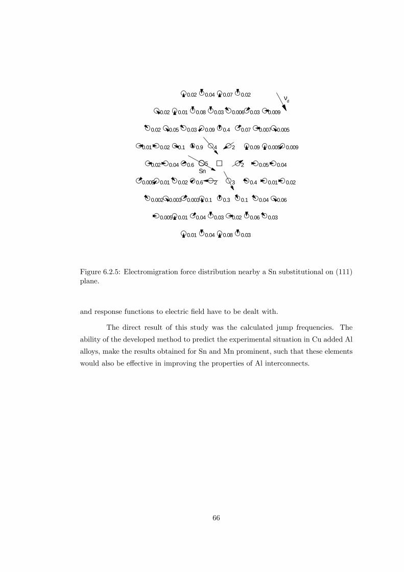
0.005 0.01

0.01

0.04 0.03

0.08

0.02

0.04

0.06 0.03

0.03

0.005 0.01

0.003

0.02

0.002

0.6

0.1

2

0.003

3

0.1

0.4

0.3

0.01

0.06

0.02

0.04

0.01

0.02

0.02 0.1

0.6

0.9

0.04

4 2 0.09

0.05

0.005

2

0.009

0.04

0.02

0.05

0.01

0.02

0.08

0.09

0.03

0.03

0.006

0.07

0.03

0.4

0.009

0.0050.007

0.02 0.070.04 0.02

5

νd

Sn

Figure 6.2.5: Electromigration force distribution nearby a Sn substitutional on (111)plane.

and response functions to electric �eld have to be dealt with.

The direct result of this study was the calculated jump frequencies. The

ability of the developed method to predict the experimental situation in Cu added Al

alloys, make the results obtained for Sn and Mn prominent, such that these elements

would also be e¤ective in improving the properties of Al interconnects.

66

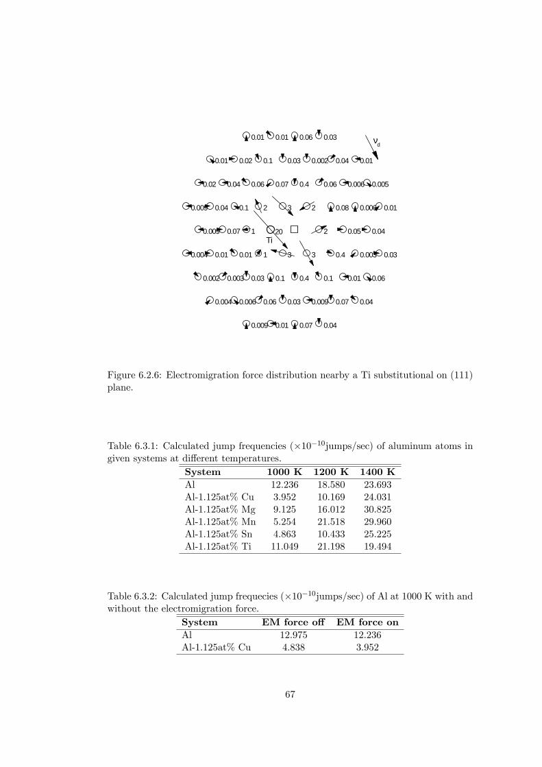
0.004 0.006

0.009

0.06 0.03

0.07

0.009

0.01

0.07 0.04

0.04

0.004 0.01

0.003

0.01

0.002

1

0.1

3

0.03

3

0.1

0.4

0.4

0.003

0.06

0.03

0.01

0.009

0.009

0.04 0.1

1

2

0.07

3 2 0.08

0.05

0.006

2

0.01

0.04

0.01

0.04

0.02

0.02

0.1

0.07

0.03

0.06

0.002

0.06

0.04

0.4

0.01

0.0050.006

0.01 0.060.01 0.03

20

νd

Ti

Figure 6.2.6: Electromigration force distribution nearby a Ti substitutional on (111)plane.

Table 6.3.1: Calculated jump frequencies (�10�10jumps/sec) of aluminum atoms ingiven systems at di¤erent temperatures.

System 1000 K 1200 K 1400 KAl 12.236 18.580 23.693Al-1.125at% Cu 3.952 10.169 24.031Al-1.125at% Mg 9.125 16.012 30.825Al-1.125at% Mn 5.254 21.518 29.960Al-1.125at% Sn 4.863 10.433 25.225Al-1.125at% Ti 11.049 21.198 19.494

Table 6.3.2: Calculated jump frequecies (�10�10jumps/sec) of Al at 1000 K with andwithout the electromigration force.

System EM force o¤ EM force onAl 12.975 12.236Al-1.125at% Cu 4.838 3.952

67

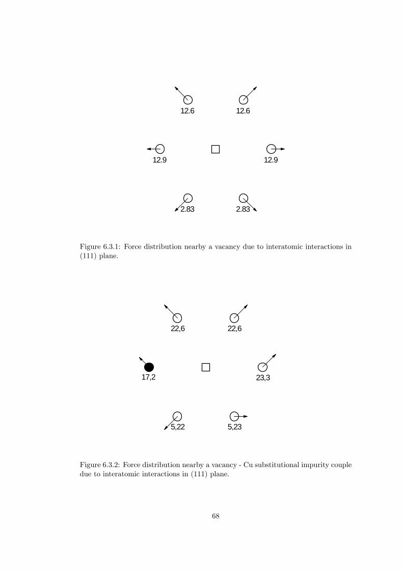
2.83 2.83

12.6 12.6

12.9 12.9

Figure 6.3.1: Force distribution nearby a vacancy due to interatomic interactions in(111) plane.

5,22 5,23

22,6 22,6

23,317,2

Figure 6.3.2: Force distribution nearby a vacancy - Cu substitutional impurity coupledue to interatomic interactions in (111) plane.

68

Chapter 7

Conclusion

In the present study, the e¤ect of alloying aluminum on the di¤usion behavior under

electromigration force was investigated using non-equilibrium molecular dynamics

simulations. The electromigration force was calculated by a pseudopotential formal-

ism and the calculated force was added to the interatomic force in the corrector

stage of the molecular dynamics. It is shown in this study that the developed proce-

dure can be used to understand the electromigration processes occurring in metallic

interconnect alloys.

Heine-Abarenkov-Animalu model potentials were used in the atomic interactions.

The potentials were tested for the aluminum such that some of the ground state prop-

erties were calculated and compared with the experimental values. The calculated

properties were found to be close to the experimental values where, lattice parameter

was obtained with 2.96% error and self-di¤usion activation energy for aluminum was

found to be 67.6 kJ/mole.

Various alloying elements were added to the aluminum and the corresponding

electromigration force on the alloying elements were determined. It has been found

that the force on Cu, Li, Na and Pd is smaller compared to other elements. In

transition metals there is a direct relation between the electron scattering force and

the chemical valence of the element.

The change in the jump frequencies of aluminum atoms were reported at di¤erent

temperatures by addition of Cu, Mg, Mn, Sn and Ti to the aluminum. It was found

that, Cu, Mn and Sn reduces the kinetics of the jumps of aluminum atoms. Therefore,

it is suggested that Cu, Mn and Sn can be used as an alloying element to improve

the resistance of aluminum to electromigration. Thus longer failure times and an

increase in the reliability of the interconnects can be achieved.

69

References

[1] N. Metropolis, A. W. Rosenbluth, M. N. Rosenbluth, A. H. Teller, and E. Teller.

Equation of state calculations by fast computing machines. Journal of Chemical

Physics, 21:1087�92, 1953.

[2] B. J. Alder and T.E. Wainwright. Phase transition for a hard sphere system.

Journal of Chemical Physics, 27:1208�9, 1957.

[3] B. J. Alder and T. E. Wainwright. Studies in molecular dynamics. Journal of

Chemical Physics, 31:459�66, 1959.

[4] A. Rahman. Correlations in the motion of atoms in liquid argon. Physical

Review, 136:A405, 1964.

[5] G. Sutmann. Classical molecular dynamics. Quantum Simulations of Complex

Many-Body Systems: From Theory to Algorithms, Lecture Notes, 10:211�254,

2002.

[6] A. Davuto¼glu. Molecular Dynamics Studies of Di¤usion Behaviour in

Aluminum-Copper Metals and Alloys. PhD thesis, Middle East Technical Uni-

versity, September 2003.

[7] K. P. Travis. Simulation of the Liquid State, chapter 6, pages 217�270. Royal

Society of Chemistry, 2004.

[8] W. G. Hoover and W. T. Ashurst. Theoretical Chemistry: Advances and Per-

spectives, volume 1, chapter Nonequilibrium molecular dynamics, pages 1�51.

Academic Press, New York, 1975.

[9] D. J. Evans and G. P. Morris. Statistical Mechanics of Nonequilibrium Liquids.

Academic Press, New York, 1990.

[10] J. R. Lloyd. Electromigration for designers: An introduction for the non spe-

cialist. Technical report, IBM TJ Watson Research Center, 2002.

70

[11] D. R. Fridline and A. F. Bower. In�uence of anisotropic surface di¤usivity

on electromigration induced void migration and evolution. Journal of Applied

Physics, 85:3168, 1999.

[12] J. P. Dekker, C. A. Volkert, E. Arzt, and P. Gumbsch. Alloying e¤ects on

electromigration mass transport. Physical Review Letters, 87(3):035901, 2001.

[13] T. A. Ogurtani and E. E. Oren. Computer simulation of void growth dynamics

under the action of electromigration and capillary forces in narrow thin inter-

connects. Journal of Applied Physics, 90(3):1564, 2001.

[14] R. S. Sorbello. A pseudopotential based theory of the driving forces for electro-

migration in metals. Journal of Physics and Chemistry of Solids, 34:937�950,

1972.

[15] R. S. Sorbello. Atomic con�guration e¤ects in electromigration. Journal of

Physics Chemistry of Solids, 42:309�316, 1980.

[16] P. Kumar and R. S. Sorbello. Linear response theory of the driving forces for

electromigration. Thin Solid Films, 25:25�35, 1975.

[17] T. Ohkubo, Y.Hirotsu, and K.Nikawa. Molecular dynamics simulation of electro-

migration in nano-sized metal lines. Materials Transactions, JIM, 37(3):454�457,

1996.

[18] T. Shinzawa and T. Ohta. Molecular dynamics simulation of al grain boundary

di¤usion for electromigration failure analysis. In Proceedings of the IEEE 1998

International Interconnect Technology Conference, 1998.

[19] D. Maroudas and M. R. Gungor. Continuum and atomistic modeling of

electromechanically-induced failure of ductile metallic thin �lms. Computational

materials science, 23:242�249, 2002.

[20] J. B. Gibson, A. N. Goland, M. Milgram, and G. H. Vineyard. Dynamics of

radiation damage. Physical Review, 120:1229�1253, 1960.

[21] L. Verlet. Computer �experiments�on classical �uids. i. thermodynamical prop-

erties of lennard-jones molecules. Physical Review, 159:98�103, 1967.

[22] L. Verlet. Computer �experiments�on classical �uids. II. equilibrium correlation

functions. Physical Review, 165:201�214, 1968.

71

[23] F. Ercolessi. A molecular dynamics primer. http://www.sissa.it/furio/md, 2006.

[24] A. Münster. Statistical Thermodynamics. Springer/Academic Press, Berlin/New

York, 1969.

[25] I. M. Torrens. Interatomic Potentials. Academic Press, New York, 1972.

[26] M. P. Allen and D. J. Tildesley. Computer Simulation of Liquids. Oxford Uni-

versity Press, New York, 1987.

[27] M. P. Allen. Introduction to molecular dynamics simulation. Computational Soft

Matter: From Synthetic Polymers to Proteins, Lecture Notes, 23:1�28, 2004.

[28] R. W. Hockney and J. W. Eastwood. Computer Simulations Using Particles.

Adam Hilger, Bristol, 1988.

[29] W. C. Swope, H. C. Andersen, P. H. Berens, and K. R. Wilson. A computer

simulation method for the calculation of equilibrium constants for the formation

of physical clusters of molecules: Application to small water clusters. Journal of

Chemical Physics, 76:637�649, 1982.

[30] C. W. Gear. The numerical integration of ordinary di¤erential equations of var-

ious orders. Technical Report Report ANL 7126, Argonne National Laboratory,

1966.

[31] C. W. Gear. Numerical Initial Value Problems in Ordinary Di¤erential Equa-

tions. Prentice-Hall, Englewood Cli¤s, NJ, 1971.

[32] M. Born and Th. Von Karman. über schwingungen in raumgittern. Physik. Z.,

13:297�309, 1912.

[33] D. W. Heermann. Computer Simulation Methods in Theoretical Physics.

Springer-Verlag, Germany, 1990.

[34] L. V. Woodcock. Isothermal molecular dynamics calculation for liquid salt.

Chemical Physics Letters, 10:257�261, 1971.

[35] H. J. C. Berendsen, J. P. M. Postma, W. F. Van Gusteren, A. DiNola, and

J. R. Haak. Molecular dynamics with coupling to an external bath. Journal of

Chemical Physics, 81(8):3684�3690, 1984.

[36] S. Nose. A molecular dynamics method for simulations in the canonical ensemble.

Molecular Physics, 52:255�268, 1984.

72

[37] W. H. Hoover. Canonical dynamics: Equilibrium phase-space distributions.

Physical Review A, 31(3):1695�1697, 1985.

[38] W. G. Hoover. Constant pressure equations of motion. Physical Review A,

34:2499�2500, 1986.

[39] S. Nose. An extension of the canonical ensemble molecular dynamics method.

Molecular Physics, 57:187�191, 1986.

[40] R. Windiks. Thermostatting in molecular dynamics simulations.

http://homepage.swissonline.ch/windiks/documents/thermostats.pdf, 2006.

[41] H. C. Andersen. Molecular dynamics simulations at constant pressure and/or

temperature. Journal of Chemical Physics, 72:2384�2393, 1980.

[42] J. M. Haile and H. W. Graben. Molecular dynamics simulations extended to

various ensembles. i. equilibrium properties in the isoenthalpic-isobaric ensemble.

Journal of Chemical Physics, 73:2412�2419, 1980.

[43] A. Hinchli¤e. Chemical Modelling from Atoms to Liquids. John Wiley and Sons

Ltd, 1999.

[44] H. J. C. Berendsen and W. F. Van Gusteren. Practical algorithms for dynamic

simulations. molecular dynamics simulation of statistical mechanical systems. In

Proceedings of the Enrico Fermi Summer School, pages 43�65, Bologna, 1986.

Soc. Italiana di Fisica.

[45] A. R. Leach. Molecular Modelling Principles and Applications. Addison Wesley

Longman Limited, 1996.

[46] D. J. Evans and G. P. Morriss. Non-newtonian molela dynamics. Computer

Physics Reports, 1(6):297�343, 1984.

[47] J. J. Erpenbeck and W. W. Wood. Molecular dynamics techniques for hard core

particles. In B. J. Berne, editor, Statistical Mechanics B. Modern Theoretical

Chemistry, pages 1�40. Plenum, New York, 1977.

[48] A. A. Katsnelson, V. S. Stepanyuk, A. I. Szasz, and O. V. Farberovich. Com-

putational Methods in Condensed Matter: Electronic Structure. AIP, New York,

1992.

[49] D. R. Hamann, M. Schlüter, and C. Chiang. Norm-conserving pseudopotentials.

Physical Review Letters, 43:1494�1497, 1979.

73

[50] D. R. Hamann. Generalized norm-conserving pseudopotentials. Physical Review

B, 40:2980�2987, 1989.

[51] A. M. Rappe, K. M. Rabe, E. Kaxiras, and J. D. Joannopoulos. Optimized

pseudopotentials. Physical Review B, 41:1227�1230, 1990.

[52] N. Troulier and J. L. Martins. E¢ cient pseudopotentials for plane-wave calcu-

lations. Physical Review B, 43:1993�2006, 1991.

[53] D. Vanderbilt. Optimally smooth norm-conserving pseudopotentials. Physical

Review B, 32:8412�8415, 1985.

[54] M. Fuchs and Sche­ er. Ab initio pseudopotentials for electronic structure cal-

culations of poly-atomic systems using density-functional theory. Computational

Physics Communications, 119:67, 1999.

[55] N. W. Ashcroft. Electron-ion pseudopotentials in metals. Physical Letters, 23:48,

1966.

[56] V. Heine and I. V. Abarenkov. New method for electronic structure of metals.

Philosophical Magazine, 9:451, 1964.

[57] I. V. Abarenkov and V. Heine. Model potential for positive ions. Philosophical

Magazine, 12:529, 1965.

[58] A. O. E. Animalu. Electronic structure of transition metals. II. phonon spectra.

Physical Review B, 8:3542, 1973.

[59] W. A. Harrison and J. M. Wills. Interionic interactions in simple metals. Physical

Review B, 25:5007, 1982.

[60] V. N. Antonov, V. Y. Milman, V. V. Nemoshkalenko, and A. V. Zhalkotitarenko.

Lattice-dynamics of fcc transition-metals-a pseudopotential approach. Zeitschrift

fur Physik B - Condensed Matter, 79:223, 1990.

[61] C. Fiolhais, J. P. Perdew, S. Q. Armster, J. M. MacLaren, and M. Brajczewska.

Dominant density parameters and local pseudopotentials for simple metals.

Physical Review B, 51:14001, 1995.

[62] J. L. Bretonnet, G. M. Bhuiyan, and M. Silbert. Gibbs-bogoliubov variational

scheme calculations for the liquid structure of 3d transition metals. Jornal of

Physics Condensed Matter, 4:5359, 1992.

74

[63] J. L. Bretonnet and M. Silbert. Interionic interactions in transition-metals-

application to vanadium. Physics and Chemistry of Liquids, 24:169, 1992.

[64] M. Hasegawa, K. Hoshino, and M. Watabe. A new simple pseudopotential with

applications to liquid-metal structure factor. Journal of Non-Crystalline Solids,

117/118:300, 1990.

[65] A. O. E. Animalu and V. Heine. The screened model potential for 25 elements.

Philosophical Magazine, 12:1249, 1965.

[66] A. O. E. Animalu. The total electronic band structure energy for 29 elements.

Proceedings of the Royal Society of London Series A, Mathematical and Physical

Sciences, 294(1438):376�392, 1966.

[67] J. Lindhard. On the properties of a gas of charged particles. Matematisk-fysiske

meddelelser Kongelige Danske Videnskabernes Selskab, 28(8), 1954.

[68] J. Hubbard. The description of collective motions in terms of many-body pertur-

bation theory.2.the correlation energy of a free-electron gas. Proceedings of the

Royal Society of London Series A-mathematical and physical sciences, A243:336,

1958.

[69] L. Kleinman. New approximation for screened exchange and the dielectric con-

stant of metals. Physical Review, 160:585, 1967.

[70] D. J. W. Geldart and S. H. Vosko. Screening function of an interacting electron

gas. Canadian Journal of Physics, 44:2137, 1966.

[71] D. C. Langreth. Approximate screening functions in metals. Physical Review,

181:753, 1969.

[72] S. Ichimaru and K. Utsumi. Analytic expression for the dielectric screening

function of strongly coupled electron liquids at metallic and lower densities.

Physical Review B, 24:7385, 1981.

[73] P. Vashista and K. S. Singwi. Electron correlations at metallic densities. Physical

Review B, 6:875, 1972.

[74] S. Moronoi, D. M. Ceperley, and G. Senatore. Static response and local �eld

factor of the electron gas. Physical Review Letters, 75:689, 1995.

[75] P. S. Ho and T. Kwok. Electromigration in metals. Reports on Progress in

Physics, 52:301�348, 1989.

75

[76] R. S. Sorbello. Theory of electromigration. In Solid State Physics, volume 51,

pages 159�231. Academic�New York, 1997. Vol 51.

[77] V. B. Fiks. On the mechanism of the mobility of ions in metals. Soviet Physics

-Solid State, 1:14, 1959.

[78] H. B. Huntington and A. R. Grone. Current induced marker motion in gold

wires. Journal of Physics and Chemistry of Solids, 20:76, 1961.

[79] C. Bosvieux and J. Friedel. Sur leelectrolyse des alliages metalliques. Journal of

Physics and Chemistry of Solids, 20:76, 1961.

[80] T. N. Todorov, J. Hoekstra, and A. P. Sutton. Current-induced forces in atomic-

scale conductors. Philosophical Magazine B, 80(3):421�455, 2000.

[81] J. P. Dekker and A. Lodder. Calculated electromigration wind force in face-

centered-cubic and body-centered-cubic metals. Journal of Applied Physics,

4:1958, 1998.

[82] J. D. Gale and A. L. Rohl. The general utility lattice program. Molecular

Simulation, 29:291, 2003.

[83] K. N. Tu. Recent advances on electromigration in very-large-scale-integration of

interconnects. Journal of applied physics, 94(9):5451�5473, 2003.

[84] J. Bandyopadhyay and K. P. Gupta. Low temperature lattice parameters of al

and al-zn alloys and grüneisen parameter of al. Cryogenics, London, 18:54�55,

1978.

[85] C. Kittel. Introduction to Solid State Physics. John Wiley and Sons, New York,

1986.

[86] G. Simmons and H. Wang. Single-Crystal Elastic Constants and Calculated

Aggregate Properties: A Handbook. MIT Press, MA, 1971.

[87] S. Dais, R. Messer, and A. Seeger. Nuclear-magnetic-resonance study of self-

di¤usion in aluminum. Materials Science Forum, 15-18:419�424, 1987.

76

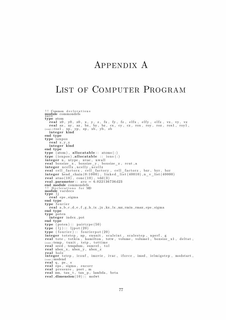
Appendix A

List of Computer Program

! ! Common d e c l e r a t i o n smodule commondefssavetype atomreal x0 , y0 , z0 , x , y , z , fx , fy , f z , e l f x , e l f y , e l f z , vx , vy , vzreal ax , ay , az , bx , by , bz , cx , cy , cz , rox , roy , roz , rox1 , roy1 ,

(cont.) roz1 , xp , yp , zp , xb , yb , zbinteger kind

end typetype i onposreal x , y , zinteger kind

end typetype ( atom ) , al locatable : : atoms ( : )type ( i onpos ) , al locatable : : i o n s ( : )integer n , ntype , nvac , nwa l lreal boxsize_x , boxsize_y , boxsize_z , rcut , ainteger n c e l l x , n c e l l y , n c e l l zreal c e l l_ f a c t o r x , c e l l_ f a c t o r y , c e l l_ f a c t o r z , bxr , byr , bzrinteger head_chain ( 0 : 1 0 0 0 ) , l i n k e d_ l i s t (40010) , n_v_list (40000 )real atno (10 ) , conc (10 ) , vdd ( 3 )real , parameter : : avo = 6 .022136736 d23end module commondefs! ! D e c l e r a t i o n s f o r MDmodule vardec stype l jreal eps , sigma

end typetype f o u r i e rreal a , b , c , d , e , f , g , h , ix , jx , kx , lx ,mx, rmin , rmax , eps , sigma

end typetype poteninteger index , pot

end typetype ( poten ) : : p a i r t yp e (50 )type ( l j ) : : l j p o t ( 20 )type ( f o u r i e r ) : : f o u r i e r p o t ( 20 )integer t o t s t ep , np , enunit , s c a l e i n t , s c a l e s t e p , nper f , greal to te , t o tk in , hamilton , totw , volume , volume1 , boxsize_x1 , d e l t a t ,(cont.) temp , tun i t , t s tp , t o t t imereal seed , tempdum , sumvel , t o lreal nbox_x , nbox_y , nbox_zreal bo l zinteger t s t ep , i c on f , imovie , ivac , i f o r c e , imsd , i e lm i g s t e p , msdstart ,(cont.)msdendreal q , ps , sreal eps , sigma , en co r rreal pre s su r e , pset , mreal mu, tau_t , tau_p , lambda , betareal , dimension ( 10 ) : : molwt

77

real , al locatable : : x i n i ( : ) , y i n i ( : ) , z i n i ( : )real , parameter : : p i = 3 .14159265358979end module vardec s! ! D e c l e r a t i o n s f o r EM f o r c e r o u t i n eModule Defssavetype e l ementsinteger atnocharacter ( 2 ) namereal a0 , a1 , a2 , rm , om, m, rc , a l f , ec , cinteger z

end typetype ( e l ements ) : : sp ( 10 )type ( e l ements ) : : e l ( 5 6 )real rr , r r d i r ( 3 ) , omave , zave , mave , x , y , z , box_x , box_y , box_z ,(cont.) c u t o f f , xr , yr , z rreal kf , e f , v f , vd , vdd i r ( 3 ) , r s , k s iinteger i1 , i2 , f o r c e_ j , f o r c e_ ireal , parameter : : PI = 3.14159265358979end module Defs! ! MD p ro g r amprogram mduse vardec suse commondefsreal rp , r0 , msdreal d e l t a t s q , hde l t a t sq , boxsize_x2 , boxsize_y2 , boxs ize_z2real e l ap s ed t imereal pavr , sumpreal t o t e i , t o t k i n iinteger i , c ounte rreal , external : : t ime f , read_contro l , open_output , f c c2 , i n i t v e l ,(cont.) f o r c e e v a l , nh1 , nh2 , e lmig , new_nlist , f indvac , va c fcharacter c o n t r o l f i l e � 12integer ( 2 ) statuse l ap s ed t ime = t ime f ( )ca l l g e ta rg ( 1 , c o n t r o l f i l e , status )i f ( status . eq . �1) thenwrite (� , �) " en t e r �c o n t r o l f i l e �name�: "read (� , �) c o n t r o l f i l ei f ( c o n t r o l f i l e == ��) stopendifc a l l r ead_contro l ( c o n t r o l f i l e )ca l l open_output ( c o n t r o l f i l e , i c on f , ivac , i f o r c e , imsd , imov ie )ca l l f c c 2 ( a , i n t (nbox_x) , i n t (nbox_y) , i n t ( nbox_z ) )i f ( enun i t . eq . 0) thenbo l z = 1 .380658d�23t u n i t = 1 . 0 d�15do i =1, ntypemolwt ( i ) = molwt ( i ) / avo � 0 .001

enddoendifi f ( enun i t . eq . 1) thenbo l z = 8 .617317547d�5t u n i t = 0 .09822732370761

endif! p a r am e t e r s i n cu t� o f f c o r r e c t i o n seps = 1 .507212225d�20sigma = 2.5748426d�10p s e t = 2 . 5 d�3tau_p = 0 .01tau_t = 1 . 0beta = 0 .74474m = 1 . 0 d�5volume1 = 0 . 0counte r = 0! s e e d = 0 . 8 5np = nd e l t a t s q = ( d e l t a t ��2) � ( t u n i t ��2)hd e l t a t s q = d e l t a t s q � 0 . 5t s t p = d e l t a t � t u n i tboxs ize_x2 = boxsize_x / 2boxsize_y2 = boxsize_y / 2

78

boxs ize_z2 = boxs ize_z / 2volume = boxsize_x � boxsize_y � boxs ize_zbxr = boxsize_x / ( volume ��0 .3333333333)byr = boxsize_y / ( volume ��0 .3333333333)bzr = boxs ize_z / ( volume ��0 .3333333333)

! c u t� o f f c o r r e c t i o n sen co r r = ( 2 . 0 � p i � np / volume � 4 . 0 � eps ) � ( ( �1 . 0/9 . 0 ) � ( sigma

(cont.) ��12/ r cu t ��9) � ( �1 .0/3 .0 ) � ( sigma ��6/ r cu t ��3) )! i n i t i a l i z e p r o p e r t y v a l u e smsd = 0 . 0sumvel = 0 . 0pavr = 0 . 0! ! G i v e i n i t i a l v e l o c i t i e s t o a tom sca l l i n i t v e l ( temp )ca l l f o r c e e v a l ( np , rcut , boxsize_x , boxsize_y , boxs ize_z )

! ! �� : : n o s e�h o o v e r t h e r m o s t a t : : � � ! !s = 0 . 0g = 3 � nps = ( sumvel � real ( g ) � bo l z � temp ) / q

! i n i t i a l a c c e l e r a t i o n s , s e c o n d and t h i r d d e r i v a t i v e sdo i = 1 , natoms ( i )%ax = atoms ( i )%fx / molwt ( atoms ( i )%kind )atoms ( i )%ay = atoms ( i )%fy / molwt ( atoms ( i )%kind )atoms ( i )%az = atoms ( i )%f z / molwt ( atoms ( i )%kind )atoms ( i )%bx = 0 . 0atoms ( i )%bz = 0 . 0atoms ( i )%by = 0 . 0atoms ( i )%cx = 0 . 0atoms ( i )%cy = 0 . 0atoms ( i )%cz = 0 . 0

end dowrite ( 5 , 1 ) " to t t ime " , " poten " , " k i n e t i c " , " to t en " , "temp" , " p r e s s u r e " ,

(cont.) " hamilton " , "volume" , " d i f f u s i o n "1 format (10x , a7 , 8 a25 )! ! MD Loop

! ! ! ! ! ! ! ! ! ! ���� e q u i l i b r a t i o n ������ ! ! ! ! ! ! ! ! ! !do t s t e p = 1 , s c a l e s t e p! ! S e l e c t t h e a p p r o p r i a t e i n t e g r a t i o n r o u t i n e! ! Un comment o n l y on e o f t h e f o l l o w i n g , f o r t h e d e s i r e d e n s em b l e ,! c a l l p r e d i c t ( t s t p ) ! ! Uncomment t h i s f o r Gear 5 v a l u e! c a l l v e r l e t 1 ( t s t p ) ! ! Uncomment t h i s f o r non� r e v e r s i b l e Nose�Hoov e r

(cont.) Th e rm o s t a t! c a l l v e r l 1 ( t s t p ) ! ! Uncomment t h i s f o r t r a d i t i o n a l v e l o c i t y

(cont.) V e r l e t! c a l l a n d e r s 1 ( ) ! ! Uncomment t h i s f o r A n d e r s e n p r e s s u r e c o n t r o lca l l nh1 ( t s t p ) ! ! Uncomment t h i s f o r r e v e r s i b l e Nose�Hoov e r

(cont.) Th e rm o s t a t! pbcdo i = 1 , ni f ( atoms ( i )%x . l t . 0 . 0 ) thenatoms ( i )%x = atoms ( i )%x + boxsize_x

e lse i f ( atoms ( i )%x . gt . boxs ize_x ) thenatoms ( i )%x = atoms ( i )%x � boxsize_x

end i f! ! Uncomment t h e f o l l o w i n g l i n e s f o r PBC i n y � d i r e c t i o n! i f ( a t om s ( i )%y . l t . 0 . 0 ) t h e n! a t om s ( i )%y = atom s ( i )%y + b o x s i z e_ y

! e l s e i f ( a t om s ( i )%y . g t . b o x s i z e_ y ) t h e n! a t om s ( i )%y = atom s ( i )%y � b o x s i z e_ y

! end i fi f ( atoms ( i )%z . l t . 0 . 0 ) thenatoms ( i )%z = atoms ( i )%z + boxs ize_z

e lse i f ( atoms ( i )%z . gt . boxs ize_z ) thenatoms ( i )%z = atoms ( i )%z � boxs ize_z

end i fend doca l l f o r c e e v a l ( np , rcut , boxsize_x , boxsize_y , boxs ize_z )! ! S e l e c t t h e a p p r o p r i a t e i n t e g r a t i o n r o u t i n e! ! Uncomment o n l y t h e c o r r e c t o r s t e p o f t h e p r e v i o u s l y s e l e c t e d

(cont.) i n t e g r a t o r .

79

ca l l nh2 ( t s t p ) ! ! Uncomment t h i s f o r r e v e r s i b l e Nose�Hoov e r(cont.) Th e rm o s t a t

! c a l l a n d e r s 2 ( ) ! ! Uncomment t h i s f o r A n d e r s e n p r e s s u r e c o n t r o l! c a l l v e r l e t 2 ( t s t p ) ! ! Uncomment t h i s f o r non� r e v e r s i b l e Nose�

(cont.) Hoov e r T h e rm o s t a t! c a l l c o r r e c t ( t s t p ) ! ! Uncomment t h i s f o r Gea r 5 v a l u e! c a l l b e r e n d s e n ( ) ! ! Uncomment t h i s f o r B e r e n d s e n p r e s s u r e

(cont.) c o n t r o l! c a l l v e r l 2 ( t s t p ) ! ! Uncomment t h i s f o r t r a d i t i o n a l v e l o c i t y

(cont.) V e r l e tt o t t ime=counte r � t s t p! c a l l v e l s c a l e ( ) ! ! Uncomment t h i s f o r t e m p e r a t u r e c o n t r o l by

(cont.) v e l o c i t y s c a l i n gsumvel = 0 . 0do i = 1 ,nsumvel = sumvel + ( atoms ( i )%vx��2 + atoms ( i )%vy��2 + atoms ( i )%vz

(cont.) ��2) �molwt ( atoms ( i )%kind )end do! ! Uncomment t h e f o l l o w i n g i n a p r e s s u r e c o n t r o l l e d s i m u l a t i o n! b o x s i z e_ x = vo lum e � b x r! b o x s i z e_ y = vo lum e � b y r! b o x s i z e _ z = vo lum e � b z r

! c a l c u l a t e p r o p e r t i e st o t k i n = 0 . 5 � sumvelcounte r = counte r + 1tempdum = ( sumvel ) / (3 � real ( n ) � bo l z )p r e s s u r e = ( ( n � bo l z � tempdum) + (1 / 3) � totw ) / volumesump = sump + p r e s s u r epavr = sump / counte rt o t e i = t o t e / ( n + nwal l )t o t k i n i = t o t k i n / ( n + nwal l )hamilton = to t e + t o t k i n + ( ps ��2 � q ) / ( 2 . 0 ) + real ( g ) � tempdum

(cont.) � bo l z � swrite (� , 2 ) t s t ep , tempdum , t o t e + to tk in , hami lton2 format ( i8 , 3 e s13 . 5 )

! ! u p d a t e L i n k e d l i s tca l l new_nl ist ( )

! ! W r i t e t h e p r o p e r t i e s t o a f i l ei f ( enun i t . eq . 1) thenwrite ( 5 , 1 5 ) tot t ime , t o t e i , t o t k i n i , t o t e i + t o t k i n i + encorr ,

(cont.) tempdum , p r e s su r e , hamilton , volume15 format (1x , 8 e s25 . 1 7 )

endifi f ( enun i t . eq . 0) thenwrite ( 5 , 1 6 ) tot t ime , t o t e i , t o t k i n i , t o t e i + t o t k i n i + encorr ,

(cont.) tempdum , p r e s su r e , hamilton , volume16 format (1x , 8 e s25 . 1 7 )

endif! ! w r i t e t h e p o s i t i o n s , v e l o c i t i e s , a c c e l e r a t i o n s and v a c a n c y

(cont.) p o s i t i o n s a t i n t e r v a l si f ( i v a c . gt . 0) theni f (mod( t s t ep , i v a c ) . eq . 0) thenwrite ( 8 , �) nvacwrite ( 8 , �) " vacancy�p o s i t i o n s : �" , " at�s t ep=�" , t s t ep , "�time=�" ,

(cont.) to t t ime , "�f s "do i = n + nwal l + 1 , n + nwal l + nvacwrite ( 8 , 14) atoms ( i )%x , atoms ( i )%y , atoms ( i )%z14 format (1x , 3 f 2 0 . 1 0 )

enddoendif

endif! ! W r i t e t h e f o r c e on t h e a tom s a t i n t e r v a l si f ( i f o r c e . gt . 0) theni f (mod( t s t ep , i f o r c e ) . eq . 0) thenwrite ( 7 , �) " f o r c e s �" , " at�s t ep=�" , t s t ep , "�time=�" , tot t ime , "�f s

(cont.) "do i = 1 ,n + nwal l + nvacwrite ( 7 , 13) atoms ( i )%fx , atoms ( i )%fy , atoms ( i )%fz , atoms ( i )%

(cont.) e l f x , atoms ( i )%e l f y , atoms ( i )%e l f z13 format (1x , 6 e s15 . 7 )

80

enddoendif

endif! ! w r i t e t h e t r a j e c t o r y o f a t om s t o . x y z f i l e

i f ( imov ie . gt . 0) theni f (mod( t s t ep , imov ie ) . eq . 0) thenwrite ( 15 , �) n + nwal lwrite ( 15 , �) �md s t ep �, t s t e pdo i = 1 , n + nwal lwrite ( 15 , �( i3 , 3 f 1 0 . 4 ) �) atoms ( i )%kind , atoms ( i )%x , atoms ( i )%y ,

(cont.) atoms ( i )%zenddo

endifendif

end do! ! ! ! ! ! ! ���� p r o d u c t i o n ������ ! ! ! ! ! ! ! ! ! !! s t o r e i n i t i a l p o s i t i o n s f o r MSD c a l c u l a t i o n sdo i = 1 , natoms ( i )%x0 = atoms ( i )%xatoms ( i )%y0 = atoms ( i )%yatoms ( i )%z0 = atoms ( i )%z

end dodo t s t e p = s c a l e s t e p + 1 , t o t s t e p

! ! s t o r e f i r s t p o s i t i o n s f o r msddo i = 1 , natoms ( i )%xb = atoms ( i )%xatoms ( i )%yb = atoms ( i )%yatoms ( i )%zb = atoms ( i )%z

enddoca l l nh1 ( t s t p ) ! ! Uncomment t h i s f o r r e v e r s i b l e Nose�Hoov e r

(cont.) Th e rm o s t a t! c a l l p r e d i c t ( t s t p ) ! ! Uncomment t h i s f o r Gea r 5 v a l u e! c a l l v e r l e t 1 ( t s t p ) ! ! Uncomment t h i s f o r non� r e v e r s i b l e Nose�

(cont.) Hoov e r T h e rm o s t a t! c a l l v e r l 1 ( t s t p ) ! ! Uncomment t h i s f o r t r a d i t i o n a l v e l o c i t y

(cont.) V e r l e t! ! ����� pbc �����

do i = 1 , ni f ( atoms ( i )%x . l t . 0 . 0 ) thenatoms ( i )%x = atoms ( i )%x + boxsize_x

e lse i f ( atoms ( i )%x . gt . boxs ize_x ) thenatoms ( i )%x = atoms ( i )%x � boxsize_x

end i f! ! Uncomment t h e f o l l o w i n g l i n e s f o r PBC i n y� d i r e c t i o n! i f ( a t om s ( i )%y . l t . 0 . 0 ) t h e n! a t om s ( i )%y = atom s ( i )%y + b o x s i z e_ y

! e l s e i f ( a t om s ( i )%y . g t . b o x s i z e_ y ) t h e n! a t om s ( i )%y = atom s ( i )%y � b o x s i z e_ y

! end i fi f ( atoms ( i )%z . l t . 0 . 0 ) thenatoms ( i )%z = atoms ( i )%z + boxs ize_z

e lse i f ( atoms ( i )%z . gt . boxs ize_z ) thenatoms ( i )%z = atoms ( i )%z � boxs ize_z

end i fend do! ! E v a l u a t e F o r c e s and c a l c u l a t e e n e r g yca l l f o r c e e v a l ( np , rcut , boxsize_x , boxsize_y , boxs ize_z )i f (mod( t s t ep , i e lm i g s t e p )==0) then! ! F in d v a a c a n c i e sca l l f i n dva c ( )! ! add e l e c t r o m i g r a t i o n f o r c e ! ! ! ! !ca l l e lm ig ( )

end i f! ! EM f o r c e t o MD f o r c e

do i = 1 , natoms ( i )%fx = atoms ( i )%fx + atoms ( i )%e l f xatoms ( i )%fy = atoms ( i )%fy + atoms ( i )%e l f yatoms ( i )%f z = atoms ( i )%f z + atoms ( i )%e l f z

end do! ! S e l e c t t h e a p p r o p r i a t e i n t e g r a t i o n r o u t i n e! ! Uncomment o n l y t h e c o r r e c t o r s t e p o f t h e p r e v i o u s l y s e l e c t e d

81

(cont.) i n t e g r a t o r .ca l l nh2 ( t s t p ) ! ! Uncomment t h i s f o r non� r e v e r s i b l e Nose�

(cont.) Hoov e r T h e rm o s t a t! c a l l v e r l e t 2 ( t s t p ) ! ! Uncomment t h i s f o r non� r e v e r s i b l e Nose�

(cont.) Hoov e r T h e rm o s t a t! c a l l c o r r e c t ( t s t p ) ! ! Uncomment t h i s f o r Gea r 5 v a l u e! c a l l v e r l 2 ( t s t p ) ! ! Uncomment t h i s f o r t r a d i t i o n a l v e l o c i t y

(cont.) V e r l e tt o t t ime = counte r � t s t pi f ( imsd . ne . 0) theni f (mod( t s t ep , imsd ) . eq . 0) thenmsd = 0 . 0

! ! r e w i n d pbc f o r msd c a l c u l a t i o ndo i = 1 , natoms ( i )%xp = atoms ( i )%x + dn int ( ( atoms ( i )%xb � atoms ( i )%x ) /

(cont.) boxsize_x ) � boxsize_xatoms ( i )%yp = atoms ( i )%y + dn int ( ( atoms ( i )%yb � atoms ( i )%y ) /

(cont.) boxsize_y ) � boxsize_yatoms ( i )%zp = atoms ( i )%z + dn int ( ( atoms ( i )%zb � atoms ( i )%z ) /

(cont.) boxs ize_z ) � boxs ize_zenddo

! ! MSD c a l c u l a t i o ndo i=msdstart , msdendrp=dsq r t ( atoms ( i )%xp��2 + atoms ( i )%yp��2 + atoms ( i )%zp ��2)r0=dsq r t ( atoms ( i )%x0��2 + atoms ( i )%y0��2 + atoms ( i )%z0 ��2)msd=msd + ( rp�r0 ) ��2

enddomsd = msd / real (msdend�msdstart+1)write ( 4 , �( f 2 0 . 1 3 , 1 x , e s25 . 1 7 ) �) real ( ( t s t e p � ( s c a l e s t e p+imsd ) ) ) �

(cont.) t s tp ,msdendif

endifsumvel = 0 . 0do i = 1 , nsumvel = sumvel + ( atoms ( i )%vx��2 + atoms ( i )%vy��2 + atoms ( i )%vz

(cont.) ��2) � molwt ( atoms ( i )%kind )end do

! c a l c u l a t e p r o p e r t i e st o t k i n = 0 . 5 � sumvelcounte r = counte r + 1tempdum = ( sumvel ) / (3 � real ( n ) � bo l z )p r e s s u r e = ( ( n � bo l z � tempdum) + (1/3 ) � totw ) / volumesump = sump + p r e s s u r epavr = sump / counte rt o t e i = t o t e / ( n + nwal l )t o t k i n i = t o t k i n / ( n + nwal l )hamilton = to t e + t o t k i n + ( ps ��2 � q ) / ( 2 . 0 ) + real ( g ) � tempdum

(cont.) � bo l z � swrite (� , 3 ) t s t ep , tempdum , to te , hamilton3 format ( i8 , 3 e s13 . 5 )

! ! Upda te n e i g h b o r l i s tca l l new_nl ist ( )i f ( enun i t . eq . 1) thenwrite ( 5 , 18) tot t ime , t o t e i , t o t k i n i , t o t e i + t o t k i n i + encorr ,

(cont.) tempdum , p r e s su r e , hamilton , volume , msd18 format (1x , 9 e s25 . 1 7 )endifi f ( enun i t . eq . 0) thenwrite ( 5 , 19) tot t ime , t o t e i , t o t k i n i , t o t e i + t o t k i n i + encorr ,

(cont.) tempdum , p r e s su r e , hamilton , volume , msd19 format (1x , 9 e s25 . 1 7 )

endif! ! w r i t e t h e p o s i t i o n s , v e l o c i t i e s , a c c e l e r a t i o n s and v a c a n c y

(cont.) p o s i t i o n s a t i n t e r v a l si f ( i c o n f . gt . 0) theni f (mod( t s t ep , i c o n f ) . eq . 0) thenwrite ( 9 , �) t s t e pdo i = 1 , nwrite ( 9 , 21) atoms ( i )%x , atoms ( i )%y , atoms ( i )%z , atoms ( i )%vx ,

82

(cont.) atoms ( i )%vy , atoms ( i )%vz21 format (1x , 6 e s15 . 7 )

end doendif

endifi f ( i f o r c e . gt . 0) theni f (mod( t s t ep , i f o r c e ) . eq . 0) thenwrite ( 7 , �) " f o r c e s �" , " at�s t ep=�" , t s t ep , "�time=�" , tot t ime , "

(cont.) �f s "do i = 1 , n + nvac + nwal lwrite ( 7 , 24) atoms ( i )%fx , atoms ( i )%fy , atoms ( i )%fz , atoms ( i )%

(cont.) e l f x , atoms ( i )%e l f y , atoms ( i )%e l f z24 format (1x , 6 e s15 . 7 )

enddoendif

endifi f ( i v a c . gt . 0) theni f (mod( t s t ep , i v a c ) . eq . 0) thenwrite ( 8 , �) nvacwrite ( 8 , �) " vacancy�p o s i t i o n s : �" , " at�s t ep=�" , t s t ep , "�time=�" ,

(cont.) to t t ime , "�f s "do i = n + nwal l + 1 , n + nvac + nwal lwrite ( 8 , 22) atoms ( i )%x , atoms ( i )%y , atoms ( i )%z22 format (1x , 3 f 2 0 . 1 0 )

enddoendif

endif! ! w r i t e t h e t r a j e c t o r y o f a t om s t o . x y z f i l e

i f ( imov ie . gt . 0 ) theni f (mod( t s t ep , imov ie ) . eq . 0) thenwrite ( 15 , �) n + nwal lwrite ( 15 , �) �md s t ep �, t s t e pdo i = 1 , n + nwal lwrite ( 15 , �( i3 , 3 f 1 0 . 4 ) �) atoms ( i )%kind , atoms ( i )%x , atoms ( i )%y

(cont.) , atoms ( i )%zenddo

endifendif

enddoi f ( i c o n f . gt . 0) close ( 9 )i f ( imsd . gt . 0) close ( 4 )i f ( i f o r c e . gt . 0) close ( 7 )i f ( i v a c . gt . 0) close ( 8 )i f ( imov ie . gt . 0) close ( 1 5 )! ! C a l c u l a t e v e l o c i t y a u t o c o r r e l a t i o n f u n c t i o nca l l vac f ( c o n t r o l f i l e , t o t s t ep , s c a l e s t e p , t s tp , n , i c o n f )e l ap s ed t ime = t ime f ( )write (� , �) " t o t a l �e l ap s ed �time�i s : �" , e l ap s ed t imewrite ( 5 , �) " t o t a l �e l ap s ed �time�i s : " , e lap sedt ime , "�s e c s . "close ( 5 )

end program md! ! T h i s r o u t i n e o p e n s o u t p u t f i l e ssubroutine open_output (name1 , i c , iv , i f r c , ims , imov )integer i c , iv , i f r c , ims , imovcharacter name1 � (� )character ( len = len_trim (name1 ) ) name2name2 = tr im (name1 )open ( unit = 5 , f i l e = name2//" . out " )i f ( i c . gt . 0) open (unit = 9 , f i l e = name2//" . con" )i f ( i v . gt . 0) open (unit = 8 , f i l e = name2//" . vac " )i f ( i f r c . gt . 0) open (unit = 7 , f i l e = name2//" . e l f " )i f ( ims . gt . 0) open (unit = 4 , f i l e = name2//" .msd" )i f ( imov . gt . 0) open (unit = 15 , f i l e = name2//" . xyz" )

end subroutine open_output! ! Read i n p u t d a t asubroutine r ead_contro l ( name1 )use vardec suse commondefs

83

integer icharacter name1 � (� ) , name�22character ( len = len_trim (name1 ) ) name2integer npot , pottype , at1 , at2 , b i tname2 = tr im (name1 )open ( unit = 10 , f i l e = name2 )open ( unit = 11 , f i l e = �f c c . txt �)read ( 10 , �) n , nvac , nwa l lread ( 10 , �) ntyperead ( 10 , �) t o t s t ep , s c a l e s t e p , s c a l e i n tread ( 10 , �) d e l t a tread ( 10 , �) t o lread ( 10 , �) msdstart , msdendread ( 10 , �) tempread ( 10 , �) qread ( 10 , �) i c on f , ivac , i f o r c e , imsd , imovie , i e lm i g s t e pread ( 10 , �) enun i tread ( 10 , �) a , boxsize_x , boxsize_y , boxsize_z , r cu tread ( 10 , �) (molwt ( i ) , i = 1 , ntype )do i = 1 , ntyperead ( 10 , �) atno ( i ) , conc ( i )

enddoread ( 10 , �) vdd ( 1 ) , vdd ( 2 ) , vdd ( 3 )al locate ( atoms (n + nvac + nwal l + 150) )al locate ( i o n s (n + nvac + nwal l + 150) )do i = 1 , 50pa i r t yp e ( i )%pot = 0

enddoread ( 10 , �) npotdo i = 1 , npotread ( 10 , �) pottypese lect case ( pottype )case ( 1 ) ! l jread ( 10 , �) at1 , at2 , l j p o t ( i )%eps , l j p o t ( i )%sigmab i t = 2�� at1 + 2�� at2pa i r t yp e ( b i t )%index = ipa i r t yp e ( b i t )%pot = 1

case ( 2 ) ! f o u r i e r p o t e n t i a lread ( 10 , �) at1 , at2 , f o u r i e r p o t ( i )%a , f o u r i e r p o t ( i )%b ,

(cont.) f o u r i e r p o t ( i )%c , f o u r i e r p o t ( i )%d , f o u r i e r p o t ( i )%e , f o u r i e r p o t ( i )%f ,(cont.) f o u r i e r p o t ( i )%g , f o u r i e r p o t ( i )%h , f o u r i e r p o t ( i )%ix , f o u r i e r p o t ( i )%jx(cont.) , f o u r i e r p o t ( i )%kx , f o u r i e r p o t ( i )%lx , f o u r i e r p o t ( i )%mx, f o u r i e r p o t ( i(cont.) )%rmin , f o u r i e r p o t ( i )%rmax , f o u r i e r p o t ( i )%eps , f o u r i e r p o t ( i )%sigma

b i t =2��at1 + 2�� at2pa i r t yp e ( b i t )%index = ipa i r t yp e ( b i t )%pot = 2

end se lectenddonbox_x = in t ( boxsize_x / a )nbox_y = in t ( boxsize_y / a )nbox_z = i n t ( boxs ize_z / a )npe r f = nbox_x � nbox_y � nbox_z � 4

! r e a d a t om i c c o o r d i n a t e sdo i = 1 ,n + nvac + nwal lread ( 1 0 , 1 0 ) atoms ( i )%kind , atoms ( i )%x , atoms ( i )%y , atoms ( i )%z10 format ( i2 , 1x , f 2 0 . 1 7 , 4x , f 2 0 . 1 7 , 4x , f 2 0 . 1 7 )

end doal locate ( x i n i ( np e r f ) , y i n i ( np e r f ) , z i n i ( np e r f ) )close ( 1 1 )n c e l l x = i n t ( boxsize_x / r cu t / 1 . 0 1 )n c e l l y = i n t ( boxsize_y / r cu t / 1 . 0 1 )n c e l l z = i n t ( boxs ize_z / r cu t / 1 . 0 1 )c e l l_ f a c t o r x = n c e l l x / boxsize_xc e l l_ f a c t o r y = n c e l l y / boxsize_yc e l l _ f a c t o r z = n c e l l z / boxs ize_zca l l new_nl ist ( )

84

ca l l ne i ghbou r_ce l l s ( )end subroutine r ead_contro l! ! T h i s r o u t i n e g i v e s i n i t i a l v e l o c i t i e s t o a tom ssubroutine i n i t v e l ( temper )use commondefsuse vardec sreal rtemp , sumx , sumy , sumzreal gauss , dummy, temper , s c a l e , sumvel2real aheat2integer idummy = 0 .5rtemp = dsq r t ( temper )aheat2 = real ( n ) � 3 . 0 � bo l z � temperdo i = 1 , natoms ( i )%vx = rtemp � gauss (dummy)atoms ( i )%vy = rtemp � gauss (dummy)atoms ( i )%vz = rtemp � gauss (dummy)

end dosumx = 0 . 0sumy = 0 . 0sumz = 0 . 0do i = 1 , nsumx = sumx + atoms ( i )%vxsumy = sumy + atoms ( i )%vysumz = sumz + atoms ( i )%vz

end dosumx = sumx / real ( n )sumy = sumy / real ( n )sumz = sumz / real ( n )do i = 1 , natoms ( i )%vx = atoms ( i )%vx � sumxatoms ( i )%vy = atoms ( i )%vy � sumyatoms ( i )%vz = atoms ( i )%vz � sumz

end dosumvel2 = 0 . 0do i = 1 ,nsumvel2 = sumvel2 + ( atoms ( i )%vx��2 + atoms ( i )%vy��2 + atoms ( i )%vz

(cont.) ��2) �molwt ( atoms ( i )%kind )end dos c a l e = dsq r t ( aheat2 / sumvel2 )sumvel = 0 . 0do i = 1 , npatoms ( i )%vx = atoms ( i )%vx � s c a l eatoms ( i )%vy = atoms ( i )%vy � s c a l eatoms ( i )%vz = atoms ( i )%vz � s c a l esumvel=sumvel + ( atoms ( i )%vx��2 + atoms ( i )%vy��2 + atoms ( i )%vz ��2) �

(cont.) molwt ( atoms ( i )%kind )end do

returnend subroutine i n i t v e l! ! T h i s f u n c t i o n g i v e s a random number i n G a u s s i a n d i s t r i b u t i o nreal function gauss (dummy)real a1 , a3 , a5 , a7 , a9parameter ( a1 = 3 .949846138 , a3 = 0 .252408784 )parameter ( a5 = 0 .076542912 , a7 = 0 .008355968 )parameter ( a9 = 0 .029899776 )real sum , r , r2real ran f , dummyinteger isum = 0 . 0do i = 1 , 12sum = sum + ran f (dummy)

enddor = (sum � 6 . 0 ) / 4 . 0r2 = r � rgauss = ( ( ( ( a9 � r2 + a7 ) � r2 + a5 ) � r2 + a3 ) � r2 +a1 ) � r

returnend function gauss! ! T h i s f u n c t i o n g e n e r a t e s a random number

85

real function r an f (dummy)integer l , c , mparameter ( l = 1029 , c = 221591 , m = 1048576)integer s eedreal dummysave seeddata s eed / 0 /seed = mod ( seed � l + c , m)r an f = real ( s eed ) / m

returnend function r an f! ! R e v e r s i b l e Nose�Hoov e r t h e r m o s t a t w i t h v e l o c i t y V e r l e t p r e d i c t o r s t e psubroutine nh1 ( dt )use vardec suse commondefsreal dt , dtsq2 , dt2 , sumvel2integer idt2 = dt / 2 . 0dtsq2 = dt � dt2sumvel2 = 0 . 0do i = 1 , nsumvel2 = sumvel2 + ( atoms ( i )%vx��2 + atoms ( i )%vy��2 + atoms ( i )%vz

(cont.) ��2) � molwt ( atoms ( i )%kind )end dops = ps + ( sumvel2 � real ( g ) � bo l z � temp ) � dt2 / qs = s + ps � dtdo i = 1 ,natoms ( i )%vx = atoms ( i )%vx � dexp(�ps � dt2 )+ ( atoms ( i )%fx / molwt (

(cont.) atoms ( i )%kind ) ) � dt2atoms ( i )%vy = atoms ( i )%vy � dexp(�ps � dt2 )+ ( atoms ( i )%fy / molwt (

(cont.) atoms ( i )%kind ) ) � dt2atoms ( i )%vz = atoms ( i )%vz � dexp(�ps � dt2 )+ ( atoms ( i )%f z / molwt (

(cont.) atoms ( i )%kind ) ) � dt2atoms ( i )%x = atoms ( i )%x + dt � atoms ( i )%vxatoms ( i )%y = atoms ( i )%y + dt � atoms ( i )%vyatoms ( i )%z = atoms ( i )%z + dt � atoms ( i )%vz

end doend subroutine nh1! ! R e v e r s i b l e Nose�Hoov e r t h e r m o s t a t w i t h v e l o c i t y V e r l e t p r e d i c t o r s t e psubroutine nh2 ( dt )use vardec suse commondefsreal dt , dt2 , sumvel2integer idt2 = dt / 2 . 0sumvel2 = 0 . 0t o t k i n = 0 . 0do i = 1 , natoms ( i )%vx = ( atoms ( i )%vx + ( atoms ( i )%fx / molwt ( atoms ( i )%kind ) ) �

(cont.) dt2 ) � dexp(�ps � dt2 )atoms ( i )%vy = ( atoms ( i )%vy + ( atoms ( i )%fy / molwt ( atoms ( i )%kind ) ) �

(cont.) dt2 ) � dexp(�ps � dt2 )atoms ( i )%vz = ( atoms ( i )%vz + ( atoms ( i )%f z / molwt ( atoms ( i )%kind ) ) �

(cont.) dt2 ) � dexp(�ps � dt2 )sumvel2 = sumvel2 + ( atoms ( i )%vx��2 + atoms ( i )%vy��2 + atoms ( i )%vz

(cont.) ��2) � molwt ( atoms ( i )%kind )end dops = ps + ( sumvel2�real ( g ) � bo l z � temp ) � dt2 / q

end subroutine nh2! ! T h i s r o u t i n e c a l c u l a t e s t h e f o r c e s f r om o f t h e i n t e r a t o m i c p o t e n t i a l(cont.) d e f i n e d on a tom s i n MDsubroutine f o r c e e v a l ( npart , rcut2 , box_x , box_y , box_z )use vardec suse commondefsreal rcut2 , box_x , box_y , box_z , rcutsq2 , box_x2 , box_y2 , box_z2 , xr , yr(cont.) , zr , x i , y i , z ireal , external : : f o r c e f un c , pot func , l e nna rd f o r c e , l enna rdene rgyinteger , external : : f i n d_ c e l lreal r x i j , r y i j , r z i j , r i j s q , r i j s q r t

86

real f i j , rp l , f x i j , f y i j , f z i jinteger npart , b i t , i , j , i c , inn , int o t e = 0 . 0totw = 0 . 0r cu t sq2 = rcu t2 ��2box_x2 = box_x / 2box_y2 = box_y / 2box_z2 = box_z / 2do i = 1 , npart + nwa l latoms ( i )%fx = 0 . 0atoms ( i )%fy = 0 . 0atoms ( i )%f z = 0 . 0

end dodo i = 1 , npart + nwa l l � 1x i = atoms ( i )%xy i = atoms ( i )%yz i = atoms ( i )%zi c = f i n d_ c e l l ( atoms ( i )%x , atoms ( i )%y , atoms ( i )%z )do inn = i n t ( i c � 27 + 1) , i n t ( i c � 27 + 27)in = n_v_list ( inn )j = head_chain ( in )do while ( j /= 0)i f ( ( j /= i ) . and . ( j >= i + 1) ) thenb i t = 2��atoms ( i )%kind + 2��atoms ( j )%kindi f ( p a i r t yp e ( b i t )%pot == 0) thenj = l i n k e d_ l i s t ( j )cycle

endifr x i j = x i � atoms ( j )%xr y i j = y i � atoms ( j )%yr z i j = z i � atoms ( j )%z

! Minimum im ag e c o n v e n t i o nxr = abs ( r x i j )yr = abs ( r y i j )z r = abs ( r z i j )i f ( xr . gt . box_x2 ) r x i j = ( xr � box_x) � s i g n ( 1 . 0 , r x i j )i f ( yr . gt . box_y2 ) r y i j = ( yr � box_y) � s i g n ( 1 . 0 , r y i j )i f ( z r . gt . box_z2 ) r z i j = ( z r � box_z ) � s i g n ( 1 . 0 , r z i j )r i j s q = ( r x i j � r x i j ) + ( r y i j � r y i j ) + ( r z i j � r z i j )r i j s q r t = dsq r t ( r i j s q )i f ( r i j s q . l t . r cu t sq2 ) thense lect case ( p a i r t yp e ( b i t )%pot )case ( 1 )f i j = l e n n a r d f o r c e ( r i j s q r t , b i t )t o t e = t o t e + lenna rdene rgy ( r i j s q r t , b i t )

case ( 2 )f i j = f o r c e f u n c ( r i j s q r t , b i t )t o t e = t o t e + pot func ( r i j s q r t , b i t )

end se lectr p l = f i j � r i j s q r tf x i j = f i j � r x i j / r i j s q r tf y i j = f i j � r y i j / r i j s q r tf z i j = f i j � r z i j / r i j s q r tatoms ( i )%fx = atoms ( i )%fx + f x i jatoms ( j )%fx = atoms ( j )%fx � f x i jatoms ( i )%fy = atoms ( i )%fy + f y i jatoms ( j )%fy = atoms ( j )%fy � f y i jatoms ( i )%f z = atoms ( i )%f z + f z i jatoms ( j )%f z = atoms ( j )%f z � f z i jtotw = totw + rp l

end i fendifj = l i n k e d_ l i s t ( j )

enddoend do

end doreturn

87

end subroutine f o r c e e v a l! ! T h i s f u n c t i o n c a l c u l a t e s p o t e n t i a l e n e r g y by F o u r i e r s e r i e sfunction pot func ( r i j , b i t )use vardec sreal pot funcreal r i j , rxinteger b i trx = p i � ( r i j � f o u r i e r p o t ( p a i r t yp e ( b i t )%index )%rmin ) / ( f o u r i e r p o t (

(cont.) pa i r t yp e ( b i t )%index )%rmax � f o u r i e r p o t ( p a i r t yp e ( b i t )%index )%rmin )pot func = f o u r i e r p o t ( p a i r t yp e ( b i t )%index )%a + f o u r i e r p o t ( p a i r t yp e ( b i t )

(cont.)%index )%b � co s ( rx ) + f o u r i e r p o t ( p a i r t yp e ( b i t )%index )%c � s i n ( rx ) +(cont.) f o u r i e r p o t ( p a i r t yp e ( b i t )%index )%d � co s ( 2 . 0 � rx ) + f o u r i e r p o t ((cont.) pa i r t yp e ( b i t )%index )%e � s i n ( 2 . 0 � rx ) + f o u r i e r p o t ( p a i r t yp e ( b i t )%(cont.) index )%f � co s ( 3 . 0 � rx ) + f o u r i e r p o t ( p a i r t yp e ( b i t )%index )%g � s i n(cont.) ( 3 . 0 � rx ) + f o u r i e r p o t ( p a i r t yp e ( b i t )%index )%h � co s ( 4 . 0 � rx ) +(cont.) f o u r i e r p o t ( p a i r t yp e ( b i t )%index )%ix � s i n ( 4 . 0 � rx ) + f o u r i e r p o t ((cont.) pa i r t yp e ( b i t )%index )%jx � co s ( 5 . 0 � rx ) + f o u r i e r p o t ( p a i r t yp e ( b i t )%(cont.) index )%kx � s i n ( 5 . 0 � rx ) + f o u r i e r p o t ( p a i r t yp e ( b i t )%index )%lx � co s(cont.) ( 6 . 0 � rx ) + f o u r i e r p o t ( p a i r t yp e ( b i t )%index )%mx � s i n ( 6 . 0 � rx )returnend function pot func! ! T h i s f u n c t i o n c a l c u l a t e s t h e f o r c e by F o u r i e r s e r i e sfunction f o r c e f u n c ( r i j 2 , b i t )use vardec sreal f o r c e f u n creal r i j 2 , y , ryinteger b i try = p i � ( r i j 2 � f o u r i e r p o t ( p a i r t yp e ( b i t )%index )%rmin ) / ( f o u r i e r p o t ((cont.) pa i r t yp e ( b i t )%index )%rmax � f o u r i e r p o t ( p a i r t yp e ( b i t )%index )%rmin )y = p i / ( f o u r i e r p o t ( p a i r t yp e ( b i t )%index )%rmax � f o u r i e r p o t ( p a i r t yp e ( b i t(cont.) )%index )%rmin )f o r c e f u n c = f o u r i e r p o t ( p a i r t yp e ( b i t )%index )%b � s i n ( ry ) � y �(cont.) f o u r i e r p o t ( p a i r t yp e ( b i t )%index )%c � co s ( ry ) � y + 2 . 0 � f o u r i e r p o t ((cont.) pa i r t yp e ( b i t )%index )%d � s i n ( 2 . 0 � ry ) � y � 2 . 0 � f o u r i e r p o t ((cont.) pa i r t yp e ( b i t )%index )%e � co s ( 2 . 0 � ry ) � y + 3 . 0 � f o u r i e r p o t ((cont.) pa i r t yp e ( b i t )%index )%f � s i n ( 3 . 0 � ry ) � y � 3 . 0 � f o u r i e r p o t ((cont.) pa i r t yp e ( b i t )%index )%g � co s ( 3 . 0 � ry ) � y + 4 . 0 � f o u r i e r p o t ((cont.) pa i r t yp e ( b i t )%index )%h � s i n ( 4 . 0 � ry ) � y � 4 . 0 � f o u r i e r p o t ((cont.) pa i r t yp e ( b i t )%index )%ix � co s ( 4 . 0 � ry ) � y + 5 . 0 � f o u r i e r p o t ((cont.) pa i r t yp e ( b i t )%index )%jx � s i n ( 5 . 0 � ry ) � y � 5 . 0 � f o u r i e r p o t ((cont.) pa i r t yp e ( b i t )%index )%kx � co s ( 5 . 0 � ry ) � y + 6 . 0 � f o u r i e r p o t ((cont.) pa i r t yp e ( b i t )%index )%lx � s i n ( 6 . 0 � ry ) � y � 6 . 0 � f o u r i e r p o t ((cont.) pa i r t yp e ( b i t )%index )%mx � co s ( 6 . 0 � ry ) � yreturnend function f o r c e f u n c! ! C a l c u l a t e f o r c e s i f L enna rd�J o n e s p o t e n t i a l i s u s e dfunction l e n n a r d f o r c e ( r i j 3 , b i t )use vardec sinteger b i treal l e nn a rd f o r c e , r i j 3l e n n a r d f o r c e = 24 � l j p o t ( p a i r t yp e ( b i t )%index )%eps � (2 � ( l j p o t ((cont.) pa i r t yp e ( b i t )%index )%sigma ��12 / r i j 3 ��13) � ( l j p o t ( p a i r t yp e ( b i t )%(cont.) index )%sigma ��6 / r i j 3 ��7) )returnend function l e n n a r d f o r c e! ! T h i s f u n c t i o n c a l c u l a t e s t h e p o t e n t i a l e n e r g y i f L enna rd�J on ed(cont.) p o t e n t i a l i s u s e dfunction l enna rdene rgy ( r i j , b i t )use vardec sinteger b i treal l ennardenergy , r i jl enna rdene rgy = 4 � l j p o t ( p a i r t yp e ( b i t )%index )%eps � ( ( l j p o t ( p a i r t yp e ( b i t(cont.) )%index )%sigma / r i j ) ��12 � ( l j p o t ( p a i r t yp e ( b i t )%index )%sigma / r i j )(cont.) ��6)returnend function l enna rdene rgy! ! T h i s r o u t i n e f i n d s t h e c e l l o f atom i n l i n k e d l i s tinteger function f i n d_ c e l l ( ionx , iony , i on z )

88

use commondefsreal ionx , iony , i on zinteger ix , iy , i zi x = i n t ( ionx � c e l l_ f a c t o r x )i y = i n t ( iony � c e l l_ f a c t o r y )i z = i n t ( i on z � c e l l _ f a c t o r z )f i n d_ c e l l = i x + iy � n c e l l x + i z � n c e l l x � n c e l l y

end function f i n d_ c e l l! ! L i n k e d l i s tsubroutine ne i ghbou r_ce l l s ( )use commondefsinteger ix , iy , i z , i c , in , i t e l , i cx , i cy , i c z , i c cx , i c cy , i c c zdo i c = 0 , n c e l l x � n c e l l y � n c e l l z � 1i t e l = 0i c z = i c / ( n c e l l x � n c e l l y )i c y = ( i c � i c z � n c e l l x � n c e l l y ) / n c e l l xi c x = ( i c � i c y � n c e l l x � i c z � n c e l l x � n c e l l y )do i z = �1, 1i c c z = i c z + i zi f ( i c c z < 0) theni c c z=i c c z+n c e l l z

e lse i f ( i c c z >= n c e l l z ) theni c c z = i c c z � n c e l l z

endifdo i y = �1, 1i c c y = i c y + iyi f ( i c c y < 0) theni c c y = i c c y + n c e l l y

e lse i f ( i c c y >= n c e l l y ) theni c c y = i c c y � n c e l l y

endifdo i x = �1, 1i c c x=i c x+ixi f ( i c c x < 0) theni c c x = i c c x + n c e l l x

e lse i f ( i c c x >= n c e l l x ) theni c c x = i c c x � n c e l l x

endifin = ( i c c x + i c c y � n c e l l x + i c c z � n c e l l x � n c e l l y )i t e l = i t e l + 1n_v_list ( i n t ( i c � 27 + i t e l ) ) = in

enddoenddo

enddoenddo

end subroutine ne i ghbou r_ce l l s! ! T h i s r o u t i n e c o n s t r u c t l i n k e d l i s tsubroutine new_nl ist ( )use commondefsinteger i , i cinteger , external : : f i n d_ c e l ldo i c = 0 , n c e l l x � n c e l l y � n c e l l z � 1head_chain ( i c ) = 0

enddodo i = 1 , n + nwal li c = f i n d_ c e l l ( atoms ( i )%x , atoms ( i )%y , atoms ( i )%z )l i n k e d_ l i s t ( i ) = head_chain ( i c )head_chain ( i c ) = i

enddoend subroutine new_nl ist! ! ! T h i s r o u t i n e i s t h e i n i t i a l i z a t i o n p a r t o f t h e e l e c t r o m i g r a t i o n(cont.) p ro g ramsubroutine i n i t ( )use d e f suse commondefsinteger i , jvd = dsq r t ( vdd ( 1 ) ��2 + vdd (2 ) ��2 + vdd (3 ) ��2)vdd i r ( 1 ) = vdd (1 ) / vdvdd i r ( 2 ) = vdd (2 ) / vdvdd i r ( 3 ) = vdd (3 ) / vddo i = 1 , ntype

89

do j = 1 , 56i f ( atno ( i ) . eq . e l ( j )%atno ) sp ( i ) = e l ( j )

enddoenddobox_x = boxsize_x / 0 .529177box_y = boxsize_y / 0 .529177box_z = boxs ize_z / 0 .529177c u t o f f = rcu t / 0 .529177do i = 1 , n + nvac + nwal li o n s ( i )%x = atoms ( i )%x / 0 .529177249i o n s ( i )%y = atoms ( i )%y / 0 .529177249i o n s ( i )%z = atoms ( i )%z / 0 .529177249i o n s ( i )%kind = atoms ( i )%kind

enddoclose ( 6 )omave = 0 . 0zave = 0 . 0mave = 0 . 0do i= 1 , ntypeomave = omave + conc ( i ) � sp ( i )%omzave = zave + conc ( i ) � sp ( i )%zmave = mave + conc ( i ) � sp ( i )%m

enddomave = 1 . 0k f = (3 � p i � p i � zave / omave ) ��0 .33333333333333v f = k f / mavee f = k f � k f / 2 / maver s = mave � ( 3 . 0 � omave / 4 . 0 / p i / zave ) ��0 .33333333333333k s i = 2 . 0 / ( 1 . 0 + 0 .02544716775 � r s )do i= 1 , n + nwal latoms ( i )%e l f x = 0 . 0atoms ( i )%e l f y = 0 . 0atoms ( i )%e l f z = 0 . 0

enddoend! ! T h i s f u n c t i o n c a l c u l a t e s t h e c o s i n e o f t h e a n g l e b e tw e e n vd and Rj�Rmreal function c o s s ( rx , ry , r z )use d e f sreal rx , ry , r zc o s s = rx / r r � vdd i r ( 1 ) + ry / r r � vdd i r ( 2 ) + rz / r r � vdd i r ( 3 )

end function c o s s! ! T h i s f u n c t i o n c a l c u l a t e s t h e d o t p r o d u c t o f vd and Rjreal function dotproduct ( i i , var )use d e f suse commondefsreal varinteger i ii f ( i i . eq . 1) dotproduct = vdd (1 ) � var + vdd (2 ) � y + vdd (3 ) � zi f ( i i . eq . 2) dotproduct = vdd (1 ) � x + vdd (2 ) � var + vdd (3 ) � zi f ( i i . eq . 3) dotproduct = vdd (1 ) � x + vdd (2 ) � y + vdd (3 ) � var

end function dotproduct! ! T h i s f u n c t i o n c a l c u l a t e s t h e s p h e r i c a l B e s s e l f u n c t i o nreal function b e s s e l ( q )use d e f sreal xx , qxx = q � r rb e s s e l = s i n ( xx ) / xx / xx � co s ( xx ) / xx

end function b e s s e l! ! T h i s f u n c t i o n i s u s e d f o r t h e i n t e g r a t i o n i n t h e f o r c e c a l c u l a t i o nreal function i n t e g r a n t 1 ( q )use d e f suse commondefsreal wi , wj , qreal , external : : w, b e s s e lwj = w( sp ( i o n s ( f o r c e_ j )%kind ) , q )i f ( i o n s ( f o r c e_ i )%kind . l t . 0 ) thenwi = w( sp ( 1 ) , q )

e lsewi = w( sp ( i o n s ( f o r c e_ i )%kind ) , q )

endif

90

i n t e g r a n t 1 = wj � wi � q � q � b e s s e l ( q )end function i n t e g r a n t 1real function i n t e g r a n t 2 ( q )use d e f suse commondefsreal wj , wi , qreal , external : : wwj = w( sp ( i o n s ( f o r c e_ j )%kind ) , q )wi = w( sp ( 1 ) , q )i n t e g r a n t 2 = wj � ( wj � wi ) � q � q � q

end function i n t e g r a n t 2real function i n t e g r a n t 3 ( q )use d e f suse commondefsreal wi , wj , qreal , external : : w, b e s s e lwi = w( sp ( 1 ) , q )wj = w( sp ( i o n s ( f o r c e_ j )%kind ) , q )i n t e g r a n t 3 = wi � wj � q � q � b e s s e l ( q )

end function i n t e g r a n t 3! ! T h i s i s t h e i n t e g r a t i o n r o u t i n e w i t h Gau s s q u a d r a t u r e methodreal function i n t e g r a t e ( i n t e g r a n t )use d e f sreal a , b , epsabs , e p s r e l , result , a b s e r rinteger key , neval , i e rreal , external : : i n t e g r a n texternal qaga = 0 .00001b = 2 . 0 � k f � 0 .00001epsabs = 0 . 0e p s r e l = 0 .001key = 3ca l l qag ( i n t e g r an t , a , b , epsabs , e p s r e l , key , result , ab se r r , neval ,

(cont.) i e r )i n t e g r a t e = result

end function i n t e g r a t e! ! T h i s f u n c t i o n c a l c u l a t e s t h e p o t e n t i a l u s e d i n EM f o r c e c a l c u l a t i o nreal function uu_s ( i i , var )use d e f suse commondefsreal , external : : co s s , dotproduct , i n t e g ran t1 , i n t e g ran t2 , i n t e g ran t3 ,(cont.) i n t e g r a t ereal t1 , term1 , term2 , term3 , uu , var , rx , ry , r zinteger i it1 = �omave��2 � mave � k f / 4 . 0 / p i ��3uu = 0 . 0do f o r c e_ i = 1 , n + nvac + nwal li f ( i o n s ( f o r c e_ i )%kind . ne . 1) thenrx = i on s ( f o r c e_ i )%x � xry = i on s ( f o r c e_ i )%y � yrz = i on s ( f o r c e_ i )%z � zi f ( i i . eq . 1) rx = i on s ( f o r c e_ i )%x � vari f ( i i . eq . 2) ry = i on s ( f o r c e_ i )%y � vari f ( i i . eq . 3) r z = i on s ( f o r c e_ i )%z � varxr = dabs ( rx )yr = dabs ( ry )z r = dabs ( r z )i f ( xr . gt . box_x / 2) rx = ( xr � box_x) � ds ign ( 1 . 0 , rx )

i f ( yr . gt . box_y / 2) ry = ( yr � box_y) � ds ign ( 1 . 0 , ry )i f ( z r . gt . box_z / 2) r z = ( z r � box_z ) � ds ign ( 1 . 0 , r z )r r = dsq r t ( rx � rx + ry � ry + rz � r z )i f ( r r <= c u t o f f ) theni f ( f o r c e_ i . ne . f o r c e_ j ) thenterm1 = t1 � vd / v f � c o s s (�rx , �ry , �r z ) � i n t e g r a t e (

(cont.) i n t e g r a n t 1 )i f ( i o n s ( f o r c e_ i )%kind . l t . 0 ) thenuu = uu � term1

91

e lseuu = uu + term1

endifi f ( i o n s ( f o r c e_ i )%kind . g t . 1) thenterm3 = t1 � vd / v f � c o s s (�rx , �ry , �r z ) � i n t e g r a t e (

(cont.) i n t e g r a n t 3 )uu = uu � term3

endife lseterm2 = t1 / 3 . 0 � dotproduct ( i i , var ) / v f � i n t e g r a t e (

(cont.) i n t e g r a n t 2 )uu = uu + term2

endifendif

endifenddouu_s = uu

end function uu_s! ! T h i s i s t h e main EM f o r c e r o u t i n esubroutine e lm ig ( )use d e f suse commondefsreal e r r o rreal , external : : uu_s , d f r i d r , i n i tinclude �data . h �! ! A l l u n i t s i n EM f o r c e i s i n a . u .ca l l i n i t ( )do f o r c e_ j = 1 , nx = i on s ( f o r c e_ j )%xy = i on s ( f o r c e_ j )%yz = i on s ( f o r c e_ j )%zatoms ( f o r c e_ j )%e l f x = �d f r i d r ( 1 , x , 0 . 2 , e r r o r ) � 51 .42210754 !

(cont.) c o n v e r t t o eV /Aatoms ( f o r c e_ j )%e l f y = �d f r i d r ( 2 , y , 0 . 2 , e r r o r ) � 51 .42210754atoms ( f o r c e_ j )%e l f z = �d f r i d r ( 3 , z , 0 . 2 , e r r o r ) � 51 .42210754

enddoend subroutine e lm ig! ! T h i s f u n c t i o n c a l c u l a t e s H e in e�Abarenkov�An iama lu p sp N( q )real function bofq ( e l e , q )use d e f sreal q , qrm , qrc , t1 , t2 , t3 , t4 , t5 , t6 , t7type ( e l ements ) : : e l eqrm = q � e l e%rmqrc = q � e l e%rct1 = p i / omave / q / qt2 = 8 . 0 � t1 � e l e%c / qt3 = s i n (qrm) � qrm � co s (qrm)t4 = 8 . 0 � t1 � e l e%z � co s (qrm)t5 = 4 . 0 � t1 � e l e%ec / qt6 = 24 . 0 � t1 � e l e%z � e l e%a l f / qrc / qrc / qrct7 = s i n ( qrc ) � qrc � co s ( qrc )bofq =�t2 � t3 � t4 + ( t5 � t6 ) � t7

end function bofq! ! T h i s f u n c t i o n c a l c u l a t e s H e in e�Abarenkov�An iama lu p sp N( q )real function nofq ( e l e , q )use d e f sreal q , t1 , t2 , t3 , t4 , xx , yy , co s t , c o s tpreal j0x , j1x , j2x , j3x , j0y , j1y , j2y , j 3ytype ( e l ements ) : : e l et1 = p i � e l e%rm � e l e%rm � e l e%rm / omavexx = k f � e l e%rmj0x = s i n ( xx ) / xxj1x = s i n ( xx ) / xx / xx � co s ( xx ) / xxj2x = 3 . 0 / xx � j 1x � j 0xj3x = 5 . 0 / xx � j 2x � j 1xi f ( ( q � 2 � k f ) . l e . 0 . 0 ) thenc o s t = ( 1 . 0 � q � q / 2 . 0 / k f / k f )t2 = �4.00 � t1 � ( e l e%a0 � e l e%c ) � ( j 0x � j 0x � j 1x � co s ( xx ) /xx )t3 = �12.0 � t1 � ( e l e%a1 � e l e%c ) � ( j 1x � j 1x � j 0x � j 2x ) � c o s tt4 = �20.0 � t1 � ( e l e%a2 � e l e%c ) � ( j 2x � j 2x � j 1x � j 3x ) � ( 3 . 0

92

(cont.) � c o s t � c o s t � 1) / 2 . 0e lseyy = (q � k f ) � e l e%rmj0y = s i n ( yy ) / yyj1y = s i n ( yy ) / yy / yy � co s ( yy ) / yyj2y = 3 . 0 / yy � j 1y � j 0yj3y = 5 . 0 / yy � j 2y � j 1yco s tp = ( xx � xx + yy � yy � ( q � e l e%rm) ��2) / 2 / xx / yyt2 = �8.00 � t1 � ( e l e%a0 � e l e%c ) / ( xx � xx � yy � yy ) � ( xx � j 1x

(cont.) � j 0y � yy � j 1y � j 0x )t3= �24.0 � t1 � ( e l e%a1 � e l e%c ) / ( xx � xx � yy � yy ) � ( xx � j 2x

(cont.) � j 1y � yy � j 2y � j 1x ) � co s tpt4 = �40.0 � t1 � ( e l e%a2 � e l e%c ) / ( xx � xx � yy � yy ) � ( xx �

(cont.) j 3x � j 2y � yy � j 3y � j 2x ) � ( 3 . 0 � co s tp � co s tp � 1 . 0 ) / 2 . 0end i fnofq = t2 + t3 + t4

returnend function nofq! ! T h i s c a l c u l a t i o n c a l c u l a t e s t h e u n s c r e e n e d HAA fo rm f a c t o rreal function w0( e l e , q )use d e f sreal qreal , external : : nofq , bo fqtype ( e l ements ) : : e l e! a n im a l u f o rm f a c t o r i s g i v e n i n Ry c o n v e r t i t t o a . u .w0 = ( nofq ( e l e , q ) + bofq ( e l e , q ) ) / 2 . 0

end function w0! ! T h i s c a l c u l a t i o n c a l c u l a t e s t h e s c r e e n e d HAA fo rm f a c t o rreal function w( e l e , q )use d e f sreal ggvosko , q , qq , l indhard , vc , h a r t r e ereal , external : : w0type ( e l ements ) : : e l eqq = q / 2 . 0 / k fggvosko = 0 . 5 � ( q��2 / ( q��2 + k s i � k f ��2) )l i ndha rd = �mave � k f / p i ��2 � ( 0 . 5 + ( 1 . 0 � qq ��2) / 4 . 0 / qq � l o g (

(cont.) abs ( ( 1 . 0 + qq ) / ( 1 . 0 � qq ) ) ) )vc = 4 . 0 � p i / q��2h a r t r e e = 1 . 0 � vc � l i ndha rd / ( 1 . 0 + vc � l i ndha rd � ggvosko )w = w0( e l e , q ) / h a r t r e e

end function w! ! Ths r o u t i n e f i n d t h e v a c a n c i e s i n t h e md c e l lsubroutine f i n dva c ( )use commondefsuse vardec sreal dumreal r x i j , r y i j , r z i jreal , external : : f c cinteger i , jl og i ca l f l a g 1ca l l f c c ( a , nbox_x , nbox_y , nbox_z )open ( 11 , f i l e = " f c c . t x t " )do i =1, np e r fread ( 1 1 , 1 1 ) x i n i ( i ) , y i n i ( i ) , z i n i ( i )11 format ( f 2 0 . 1 7 , 4x , f 2 0 . 1 7 , 4x , f 2 0 . 1 7 )

end doclose ( 11 )dum=1f l a g 1 =. f a l s e .do j =1, npe r fdo i =1,n+nwal lr x i j = x i n i ( j ) � atoms ( i )%xr y i j = y i n i ( j ) � atoms ( i )%yr z i j = z i n i ( j ) � atoms ( i )%zi f ( dabs ( r x i j ) . g t . t o l ) r x i j = ( dabs ( r x i j ) � boxsize_x ) � ds ign

(cont.) ( 1 . 0 , r x i j )i f ( dabs ( r y i j ) . g t . t o l ) r y i j = ( dabs ( r y i j ) � boxsize_y ) � ds ign

(cont.) ( 1 . 0 , r y i j )i f ( dabs ( r z i j ) . g t . t o l ) r z i j = ( dabs ( r z i j ) � boxs ize_z ) � ds ign

93

(cont.) ( 1 . 0 , r z i j )i f ( d sq r t ( r x i j ��2+ r y i j ��2+ r z i j ��2) . l t . ( t o l � d sq r t ( 3 . 0 ) ) ) f l a g 1 =.

(cont.) t ru e .enddoi f ( f l a g 1 . eq . . f a l s e . ) thenatoms (n + nwal l + dum)%x = x i n i ( j )atoms (n + nwal l + dum)%y = y i n i ( j )atoms (n + nwal l + dum)%z = z i n i ( j )atoms (n + nwal l + dum)%kind = �1dum = dum+1

endiff l a g 1 = . f a l s e .

enddonvac = dum�1

end subroutine f i n dva c! ! T h i s r o u t i n e c o n s t r u c t s an FCC c e l l f r om o l d d a t a u s e d i n f i n d v a csubroutine f c c ( a , nx , ny , nz )real areal , dimension ( 4 ) : : x0 , y0 , z0integer ix , iy , i z , i , nx , ny , nzreal , al locatable : : x ( : ) , y ( : ) , z ( : )al locate ( x ( nx � ny � nz � 4) , y ( nx � ny � nz � 4) , z ( nx � ny � nz � 4) )open ( 11 , f i l e = " f c c . t x t " , position = " rewind " , status = " o ld " )x0 ( 1 ) = 0 . 0y0 ( 1 ) = 0 . 0z0 ( 1 ) = 0 . 0x0 ( 2 ) = 0 . 0y0 ( 2 ) = 0 . 5 � az0 ( 2 ) =0.5 � ax0 ( 3 ) = 0 . 5 � ay0 ( 3 ) = 0 . 0z0 ( 3 ) = 0 . 5 � ax0 ( 4 ) = 0 . 5 � ay0 ( 4 ) = 0 . 5 � az0 ( 4 ) = 0 . 0do i y = �1, ny � 2do i x = 0 , nx � 1do i z = 0 , nz � 1do i = 1 , 4x ( i ) = ix � a + x0 ( i )y ( i ) = iy � a + y0 ( i )z ( i ) = i z � a + z0 ( i )write ( 1 1 , 1 0 ) x ( i ) , y ( i ) , z ( i )10 format ( f 2 0 . 1 7 , 4x , f 2 0 . 1 7 , 4x , f 2 0 . 1 7 )

end doend do

end doend doclose ( 11 )

end subroutine f c csubroutine f c c 2 ( a , nx , ny , nz )real areal , dimension ( 4 ) : : x0 , y0 , z0integer ix , iy , i z , i , nx , ny , nzreal , al locatable : : x ( : ) , y ( : ) , z ( : )al locate ( x ( nx � ny � nz � 4) , y ( nx � ny � nz � 4) , z ( nx � ny � nz � 4) )open ( 11 , f i l e = " f c c . t x t " , position = " rewind " , status = " o ld " )x0 ( 1 ) = 0 . 0y0 ( 1 ) = 0 . 0z0 ( 1 ) = 0 . 0x0 ( 2 ) = 0 . 0y0 ( 2 ) = 0 . 5 � az0 ( 2 ) =0.5 � ax0 ( 3 ) = 0 . 5 � ay0 ( 3 ) = 0 . 0z0 ( 3 ) = 0 . 5 � ax0 ( 4 ) = 0 . 5 � ay0 ( 4 ) = 0 . 5 � a

94

z0 ( 4 ) = 0 . 0do i y = �1, ny � 2do i x = 0 , nx � 1do i z = 0 , nz � 1do i = 1 , 4x ( i ) = ix � a + x0 ( i )y ( i ) = iy � a + y0 ( i )z ( i ) = i z � a + z0 ( i )write ( 1 1 , 1 0 ) x ( i ) , y ( i ) , z ( i )10 format ( f 2 0 . 1 7 , 4x , f 2 0 . 1 7 , 4x , f 2 0 . 1 7 )

end doend do

end doend doclose ( 11 )

end subroutine f c c 2! ! t e m p e r a t u r e c o n t r o l w i t h v e l o c i t y s c a l i n gsubroutine v e l s c a l e ( )use vardec suse commondefsreal s c a l e f a c t o r , s c a l e c o un tinteger isumvel = 0 . 0do i = 1 , nsumvel = sumvel + ( atoms ( i )%vx��2 + atoms ( i )%vy��2 + atoms ( i )%vz ��2)

(cont.) � molwt ( atoms ( i )%kind )end do! s c a l e v e l o c i t i e s a t s c a l e s t e p i n t e r v a l si f ( t s t e p . l e . s c a l e s t e p ) thens c a l e c o un t = mod( t s t ep , s c a l e i n t )i f ( s c a l e c o un t . eq . 0 . 0 ) thens c a l e f a c t o r = dsq r t ( 3 . 0 � n � bo l z � temp / sumvel )

! s c a l e v e l o c i t i e s t o d e s i r e d t e m p e r a t u r edo i = 1 , npatoms ( i )%vx = atoms ( i )%vx � s c a l e f a c t o ratoms ( i )%vy = atoms ( i )%vy � s c a l e f a c t o ratoms ( i )%vz = atoms ( i )%vz � s c a l e f a c t o r

end doend i f

end i fend subroutine v e l s c a l e! ! a n d e r s e n p r e s s u r e c o n t r o l w i t h v e l o c i t y V e r l e t p r e d i c t o r s t e psubroutine anders1 ( )use vardec suse commondefsreal sumrointeger isumro = 0 . 0do i = 1 , natoms ( i )%rox = atoms ( i )%x / boxsize_xatoms ( i )%roy = atoms ( i )%y / boxsize_yatoms ( i )%roz = atoms ( i )%z / boxs ize_zatoms ( i )%rox1 = atoms ( i )%vx / boxsize_xatoms ( i )%roy1 = atoms ( i )%vy / boxsize_yatoms ( i )%roz1 = atoms ( i )%vz / boxs ize_zsumro = sumro + ( atoms ( i )%rox1 ��2 + atoms ( i )%roy1 ��2 + atoms ( i )%roz1

(cont.) ��2) � molwt ( atoms ( i )%kind )enddodo i = 1 , natoms ( i )%rox = atoms ( i )%rox + t s t p � atoms ( i )%rox1 + 0 . 5 � t s t p ��2 �

(cont.) ( ( atoms ( i )%fx / molwt ( atoms ( i )%kind ) ) / boxsize_x � 2 . 0 / 3 . 0 �(cont.) atoms ( i )%rox1 � volume1 / volume )

atoms ( i )%roy = atoms ( i )%roy + t s t p � atoms ( i )%roy1 + 0 . 5 � t s t p ��2 �(cont.) ( ( atoms ( i )%fy / molwt ( atoms ( i )%kind ) ) / boxsize_y � 2 . 0 / 3 . 0 �(cont.) atoms ( i )%roy1 � volume1 / volume )

atoms ( i )%roz = atoms ( i )%roz + t s t p � atoms ( i )%roz1 + 0 . 5 � t s t p ��2 �(cont.) ( ( atoms ( i )%f z / molwt ( atoms ( i )%kind ) ) / boxs ize_z � 2 . 0 / 3 . 0 �(cont.) atoms ( i )%roz1 � volume1 / volume )

atoms ( i )%rox1 = atoms ( i )%rox1 + 0 . 5 � t s t p � ( ( atoms ( i )%fx / molwt ((cont.) atoms ( i )%kind ) ) / boxsize_x � 2 . 0 / 3 . 0 � atoms ( i )%rox1 � volume1 /

95

(cont.) volume )atoms ( i )%roy1 = atoms ( i )%roy1 + 0 . 5 � t s t p � ( ( atoms ( i )%fy / molwt (

(cont.) atoms ( i )%kind ) ) / boxsize_y � 2 . 0 / 3 . 0 � atoms ( i )%roy1 � volume1 /(cont.) volume )

atoms ( i )%roz1 = atoms ( i )%roz1 + 0 . 5 � t s t p � ( ( atoms ( i )%f z / molwt ((cont.) atoms ( i )%kind ) ) / boxs ize_z � 2 . 0 / 3 . 0 � atoms ( i )%roz1 � volume1 /(cont.) volume )end dosumvel=0.0do i = 1 , natoms ( i )%x = atoms ( i )%rox � boxsize_xatoms ( i )%y = atoms ( i )%roy � boxsize_yatoms ( i )%z = atoms ( i )%roz � boxs ize_zatoms ( i )%vx = boxsize_x � atoms ( i )%rox1atoms ( i )%vy = boxsize_y � atoms ( i )%roy1atoms ( i )%vz = boxs ize_z � atoms ( i )%roz1sumvel = sumvel + ( atoms ( i )%vx��2 + atoms ( i )%vy��2 + atoms ( i )%vz ��2)

(cont.) �molwt ( atoms ( i )%kind )enddotempdum = ( sumvel ) / ( 3 . 0 � real ( n ) � bo l z )p r e s s u r e = ( ( n � bo l z � tempdum) + ( 1 . 0 / 3 . 0 ) � totw ) / volumevolume = volume + t s t p � volume1 + 0 . 5 � t s t p ��2 � ( p r e s s u r e � p s e t ) /

(cont.) mvolume1 = volume1 + 0 . 5 � t s t p � ( p r e s s u r e � p se t ) / mboxsize_x = ( volume ��0 .33333333) � bxrboxsize_y = ( volume ��0 .33333333) � byrboxs ize_z = ( volume ��0 .33333333) � bzrsumvel = 0 . 0do i = 1 , natoms ( i )%x = atoms ( i )%rox � boxsize_xatoms ( i )%y = atoms ( i )%roy � boxsize_yatoms ( i )%z = atoms ( i )%roz � boxs ize_zatoms ( i )%vx = boxsize_x � atoms ( i )%rox1atoms ( i )%vy = boxsize_y � atoms ( i )%roy1atoms ( i )%vz = boxs ize_z � atoms ( i )%roz1sumvel = sumvel + ( atoms ( i )%vx��2 + atoms ( i )%vy��2 + atoms ( i )%vz ��2)

(cont.) � molwt ( atoms ( i )%kind )enddo

end subroutine anders1! ! A n d e r s e n p r e s s u r e c o n t r o l w i t h v e l o c i t y V e r l e t c o r r e c t o r s t e psubroutine anders2 ( )use vardec suse commondefsinteger ido i = 1 , natoms ( i )%rox1 = atoms ( i )%rox1 + 0 . 5 � t s t p � ( ( atoms ( i )%fx / molwt (

(cont.) atoms ( i )%kind ) ) / boxsize_x � 2 . 0 / 3 . 0 � atoms ( i )%rox1 � volume1 /(cont.) volume )

atoms ( i )%roy1 = atoms ( i )%roy1 + 0 . 5 � t s t p � ( ( atoms ( i )%fy / molwt ((cont.) atoms ( i )%kind ) ) / boxsize_y � 2 . 0 / 3 . 0 � atoms ( i )%roy1 � volume1 /(cont.) volume )

atoms ( i )%roz1 = atoms ( i )%roz1 + 0 . 5 � t s t p � ( ( atoms ( i )%f z / molwt ((cont.) atoms ( i )%kind ) ) / boxs ize_z � 2 . 0 / 3 . 0 � atoms ( i )%roz1 � volume1 /(cont.) volume )end dosumvel = 0 . 0do i = 1 , natoms ( i )%x = atoms ( i )%rox � boxsize_xatoms ( i )%y = atoms ( i )%roy � boxsize_yatoms ( i )%z = atoms ( i )%roz � boxs ize_zatoms ( i )%vx = boxsize_x � atoms ( i )%rox1atoms ( i )%vy = boxsize_y � atoms ( i )%roy1atoms ( i )%vz = boxs ize_z � atoms ( i )%roz1sumvel = sumvel + ( atoms ( i )%vx��2 + atoms ( i )%vy��2 + atoms ( i )%vz ��2)

(cont.) � molwt ( atoms ( i )%kind )enddotempdum = ( sumvel ) / ( 3 . 0 � real ( n ) � bo l z )

96

p r e s s u r e = ( ( n � bo l z � tempdum) + ( 1 . 0 / 3 . 0 ) � totw ) / volumevolume1 = volume1 + 0 . 5 � t s t p � ( p r e s s u r e � p se t ) / m

end subroutine anders2! ! B e r e n d s e n p r e s s u r e and t em p e r a t u r e c o n t r o lsubroutine berendsen ( )use vardec suse commondefsinteger isumvel = 0 . 0do i = 1 ,nsumvel = sumvel + ( atoms ( i )%vx��2 + atoms ( i )%vy��2 + atoms ( i )%vz ��2)

(cont.) � molwt ( atoms ( i )%kind )end dotempdum = ( sumvel ) / ( 3 . 0 � real ( n ) � bo l z )p r e s s u r e = ( ( n � bo l z � tempdum) + ( 1 . 0 / 3 . 0 ) � totw ) / volumemu = (1 + ( t s t p / tau_p ) � beta � ( p r e s s u r e � p se t ) ) �� ( 1 . 0 / 3 . 0 )lambda = (1 + ( t s t p / tau_t ) � ( temp / tempdum � 1) ) �� ( 0 . 5 )do i = 1 , natoms ( i )%vx = atoms ( i )%vx + t s t p � atoms ( i )%fx / molwt ( atoms ( i )%kind

(cont.) )atoms ( i )%vy = atoms ( i )%vy + t s t p � atoms ( i )%fy / molwt ( atoms ( i )%kind

(cont.) )atoms ( i )%vz = atoms ( i )%vz + t s t p � atoms ( i )%f z / molwt ( atoms ( i )%kind

(cont.) )atoms ( i )%vx = atoms ( i )%vx � lambdaatoms ( i )%vy = atoms ( i )%vy � lambdaatoms ( i )%vz = atoms ( i )%vz � lambdaatoms ( i )%x = atoms ( i )%x + t s t p � atoms ( i )%vxatoms ( i )%y = atoms ( i )%y + t s t p � atoms ( i )%vyatoms ( i )%z = atoms ( i )%z + t s t p � atoms ( i )%vzatoms ( i )%x = atoms ( i )%x � muatoms ( i )%y = atoms ( i )%y � muatoms ( i )%z = atoms ( i )%z � mu

end doboxsize_x = boxsize_x � muboxsize_y = boxsize_y � muboxs ize_z = boxs ize_z � muvolume = volume � (mu��3)

end subroutine berendsen! ! G ea r 5 t h o r d e r i n t e g r a t i o n p r e d i c t o r s t e psubroutine p r e d i c t ( dt )use vardec suse commondefsinteger ireal c1 , c2 , c3 , c4real dtc1 = dtc2 = c1 � dt / 2 . 0c3 = c2 � dt / 3 . 0c4 = c3 � dt / 4 . 0do i = 1 , natoms ( i )%x = atoms ( i )%x + c1 � atoms ( i )%vx + c2 � atoms ( i )%ax + c3 �

(cont.) atoms ( i )%bx + c4 � atoms ( i )%cxatoms ( i )%y = atoms ( i )%y + c1 � atoms ( i )%vy + c2 � atoms ( i )%ay + c3 �

(cont.) atoms ( i )%by + c4 � atoms ( i )%cyatoms ( i )%z = atoms ( i )%z + c1 � atoms ( i )%vz + c2 � atoms ( i )%az + c3 �

(cont.) atoms ( i )%bz + c4 � atoms ( i )%czatoms ( i )%vx = atoms ( i )%vx + c1 � atoms ( i )%ax + c2 � atoms ( i )%bx + c3

(cont.) � atoms ( i )%cxatoms ( i )%vy = atoms ( i )%vy + c1 � atoms ( i )%ay + c2 � atoms ( i )%by + c3

(cont.) � atoms ( i )%cyatoms ( i )%vz = atoms ( i )%vz + c1 � atoms ( i )%az + c2 � atoms ( i )%bz + c3

(cont.) � atoms ( i )%czatoms ( i )%ax = atoms ( i )%ax + c1 � atoms ( i )%bx + c2 � atoms ( i )%cxatoms ( i )%ay = atoms ( i )%ay + c1 � atoms ( i )%by + c2 � atoms ( i )%cyatoms ( i )%az = atoms ( i )%az + c1 � atoms ( i )%bz + c2 � atoms ( i )%czatoms ( i )%bx = atoms ( i )%bx + c1 � atoms ( i )%cx

97

atoms ( i )%by = atoms ( i )%by + c1 � atoms ( i )%cyatoms ( i )%bz = atoms ( i )%bz + c1 � atoms ( i )%cz

end doreturnend subroutine p r e d i c t! ! ! T h i s r o u t i n e i s t h e c o r r e c t o r s t a g e o f t h e Gear 5 t h o r d e r(cont.) i n t e g r a t i o nsubroutine c o r r e c t ( dt )use vardec suse commondefsreal axi , ay i , a z i , corrx , corry , c o r r zreal c1 , c2 , c3 , c4real gear0 , gear1 , gear3 , gear4real cr , cv , cb , ccreal dtinteger ig ea r0 = 19 .0 / 120 .0gear1 = 3 . 0 / 4 . 0gear3 = 1 . 0 / 2 . 0gear4 = 1 . 0 / 12 . 0c1 = dtc2 = c1 � dt / 2 . 0c3 = c2 � dt / 3 . 0c4 = c3 � dt / 4 . 0c r = gear0 � c2cv = gear1 � c2 / c1cb = gear3 � c2 / c3cc = gear4 � c2 / c4do i = 1 , nax i = atoms ( i )%fx / molwt ( atoms ( i )%kind )ay i = atoms ( i )%fy / molwt ( atoms ( i )%kind )a z i = atoms ( i )%f z / molwt ( atoms ( i )%kind )c o r rx = ax i � atoms ( i )%axco r ry = ay i � atoms ( i )%ayc o r r z = a z i � atoms ( i )%azatoms ( i )%x = atoms ( i )%x + cr � co r rxatoms ( i )%y = atoms ( i )%y + cr � co r ryatoms ( i )%z = atoms ( i )%z + cr � c o r r zatoms ( i )%vx = atoms ( i )%vx + cv � co r rxatoms ( i )%vy = atoms ( i )%vy + cv � co r ryatoms ( i )%vz = atoms ( i )%vz + cv � c o r r zatoms ( i )%ax = ax iatoms ( i )%ay = ay iatoms ( i )%az = a z iatoms ( i )%bx = atoms ( i )%bx + cb � co r rxatoms ( i )%by = atoms ( i )%by + cb � co r ryatoms ( i )%bz = atoms ( i )%bz + cb � c o r r zatoms ( i )%cx = atoms ( i )%cx + cc � co r rxatoms ( i )%cy = atoms ( i )%cy + cc � co r ryatoms ( i )%cz = atoms ( i )%cz + cc � c o r r z

end doreturnend! ! v e l o c i t y V e r l e t p r e d i c t o r s t e psubroutine v e r l 1 ( dt )use vardec suse commondefsreal dt , dtsq2 , dt2integer idt2 = dt / 2 . 0dtsq2 = dt � dt2do i = 1 , npatoms ( i )%x = atoms ( i )%x + dt � atoms ( i )%vx + dtsq2 � ( atoms ( i )%fx /

(cont.)molwt ( atoms ( i )%kind ) )atoms ( i )%y = atoms ( i )%y + dt � atoms ( i )%vy + dtsq2 � ( atoms ( i )%fy /

(cont.)molwt ( atoms ( i )%kind ) )atoms ( i )%z = atoms ( i )%z + dt � atoms ( i )%vz + dtsq2 � ( atoms ( i )%f z /

98

(cont.)molwt ( atoms ( i )%kind ) )atoms ( i )%vx = atoms ( i )%vx + dt2 � ( atoms ( i )%fx / molwt ( atoms ( i )%kind

(cont.) ) )atoms ( i )%vy = atoms ( i )%vy + dt2 � ( atoms ( i )%fy / molwt ( atoms ( i )%kind

(cont.) ) )atoms ( i )%vz = atoms ( i )%vz + dt2 � ( atoms ( i )%f z / molwt ( atoms ( i )%kind

(cont.) ) )end do

returnend subroutine v e r l 1! ! v e l o c i t y V e r l e t c o r r e c t o r s t e psubroutine v e r l 2 ( dt )use vardec suse commondefsreal dt , dt2integer idt2 = dt / 2 . 0t o t k i n = 0 . 0do i = 1 , npatoms ( i )%vx = atoms ( i )%vx + dt2 � atoms ( i )%fx / molwt ( atoms ( i )%kind )atoms ( i )%vy = atoms ( i )%vy + dt2 � atoms ( i )%fy / molwt ( atoms ( i )%kind )atoms ( i )%vz = atoms ( i )%vz + dt2 � atoms ( i )%f z / molwt ( atoms ( i )%kind )t o t k i n = t o t k i n + ( atoms ( i )%vx��2 + atoms ( i )%vy��2 + atoms ( i )%vz ��2)

(cont.) � molwt ( atoms ( i )%kind )end dot o t k i n = t o t k i n � 0 . 5

returnend subroutine v e r l 2! ! T h i s r o u t i n e c a l c u l a t e s v e l o c i t y a u t o c o r r e l a t i o n f u n c t i o nsubroutine vac f ( name1 , t s t ep , s s t ep , dtime , n , i c f )real va finteger i , j , n , s tep , nsample , t s t ep , s s t ep , i c freal vx0 (n ) , vy0 (n ) , vz0 (n ) , x0 (n ) , y0 (n ) , z0 (n ) , vx (n ) , vy (n ) , vz (n )real x (n ) , y (n ) , z (n ) , v0 (n ) , r0 (n ) , dtime , t imecharacter name1 � (� )character ( len = len_trim (name1 ) ) name2name2 = tr im (name1 )va f = 0 . 0open ( unit = 3 , f i l e = name2//" . con" )open ( unit = 2 , f i l e =name2//" . va f " )read ( 3 , �) s t epdo i = 1 , nread ( 3 , 31) x0 ( i ) , y0 ( i ) , z0 ( i ) , vx0 ( i ) , vy0 ( i ) , vz0 ( i )31 format (1x , 6 e s15 . 7 )v0 ( i ) = dsq r t ( vx0 ( i ) � vx0 ( i ) + vy0 ( i ) � vy0 ( i ) + vz0 ( i ) � vz0 ( i ) )r0 ( i ) = dsq r t ( x0 ( i ) ��2 + y0 ( i ) ��2 + z0 ( i ) ��2)va f = va f + ( v0 ( i ) � v0 ( i ) ) / ( v0 ( i ) � v0 ( i ) )

end dova f =va f / real ( n )t ime = real ( ( s t ep � ( s s t e p + i c f ) ) ) � dtimensample = ( t s t e p � s s t e p ) / i c fwrite ( 2 , �) time , va fdo j = 1 , nsample � 1va f = 0 . 0read ( 3 , �) s t epdo i = 1 , nread ( 3 , 3 2 ) x ( i ) , y ( i ) , z ( i ) , vx ( i ) , vy ( i ) , vz ( i )32 format (1x , 6 e s15 . 7 )va f = va f + ( vx0 ( i ) � vx ( i ) + vy0 ( i ) � vy ( i ) + vz0 ( i ) � vz ( i ) ) / (

(cont.) v0 ( i ) � v0 ( i ) )end dova f = va f / real ( n )t ime = real ( ( s t ep � ( s s t e p + i c f ) ) ) � dtimewrite ( 2 , �) time , va f

end doclose ( 2 )

end subroutine vac f

99