Embed Size (px)
Citation preview

Ragnhild Skorpa
Hydrogen dissociation underequilibrium and non-equilibriumconditionsA study using molecular dynamics
Doctoral thesisfor the degree of Philosophiae Doctor
Trondheim, October 2014
Norwegian University of Science and TechnologyFaculty of Natural Sciences and TechnologyDepartment of Chemistry

NTNU
Norwegian University of Science and Technology
Doctoral thesisfor the degree of Philosophiae Doctor
Faculty of Natural Sciences and TechnologyDepartment of Chemistry
c© 2014 Ragnhild Skorpa.
ISBN ISBN 978-82-326-0558-3 (printed version)ISBN ISBN 978-82-326-0559-0 (electronic version)ISSN 1503-8181
Doctoral theses at NTNU, 2014:323
Printed by NTNU-trykk

Acknowledgement
First of all I would like to thank Prof. Signe Kjelstrup, who has been the mainsupervisor for this project and Prof. Em. Dick Bedeaux (co-supervisor), for lettingme take part of what turned out to be an interesting journey full of surprises andchallenging new methods. I would also like to thank both of you for always havingtime to discuss new results, and for giving quick and thorough feedback on drafts(even when I specifically ask you to only look at the plots).
Additionally, I would like to thank Prof. Thijs J. H. Vlugt at TU Delft for lettingme come and work in his group for 5 months. I learnt a lot about simulations inthat period! I would also like to thank Assoc. Prof. Jean-Marc Simon at Universityof Burgundy for valuable input in the equilibrium simulations and for letting mecome to Dijon. Jing Xu is thanked for providing the molecular dynamics code forthe potential- and force routine for the hydrogen dissociation reaction. I wouldalso like to thank Storforsk Project Transport nr. 167336 and the Department ofChemistry for financing the PhD.
To all you colleagues, both former and present. Thanks for all the coffee breaks,lunches, help and support, random walks, for listening to my frustration whenthings are not going according to the plan, and for making D3 a fun place to be!Sondre, thanks for the continuous simulation support.
Family and friends, thanks for all the fun and support these years. Odne, youalways make me smile and reminds me of what is important. You really are thebest!
i


Abstract
The aim of this thesis project was to model reactions using classical moleculardynamics simulations under both equilibrium and non-equilibrium conditions andto study the effect of the reaction on the transport properties of the system. Thedissociation of hydrogen was chosen as a model system based on its importancefor the hydrogen society, and the availability of interaction potentials to model thereaction.
According to procedures described by Stillinger and Weber, a three-particle interac-tion potential was added to the pair potential. With this it was possible to properlydescribe the dissociative reaction. Equilibrium studies was performed at differenttemperatures and densities. From this, a detailed analysis of the interaction poten-tial, the pair correlation functions and the contributions from the two- and threeparticle interactions on the overall pressure was performed. This made it possibleto determine a temperature and density range where the degree of dissociation wassignificant.
The Small System method was extended to calculate partial molar enthalpies fromfluctuations of particles and energies in a subsystem embedded in the simulationbox. It was proven that this method worked well for both reacting and non-reacting mixtures. This method was applied to the hydrogen dissociation reaction.From this the reaction enthalpy was determined as a function of temperature,pressure and composition of the reacting mixture for three different densities. Thereaction enthalpy was found to be approximately constant (460–440 kJ/mol) fora gas (0.0052 g/cm3), 410–480 kJ/mol for a compressed gas (0.0191 g/cm3) and500–320 kJ/mol for a liquid (0.0695 g/cm3) for temperatures in the range 4000-21000 K. With knowledge of the reaction enthalpy, the thermodynamic equilibriumconstant, and thus the deviation from ideality was found.
Non-equilibrium simulations was used to study the coupled transport of heat andmass both transport of hydrogen through a palladium membrane and for the dis-sociative reaction in a bulk phase. For the first case, transport coefficients had tobe estimated. For the latter case, the coefficients were determined for the first timedirectly from the fluxes in the system using non-equilibrium molecular dynamicssimulations. The transport properties for both systems were then determined fromthe coefficients. For transport across a membrane, it was illustrated how a temper-
iii

iv
ature gradient could be used to enhance and control the flux of hydrogen throughthe membrane.
Contents
1 Introduction 1
1.1 Scope . . . . . . . . . . . . . . . . . . . . . . . . . . . . . . . . . . . 1
1.2 The hydrogen dissociation reaction . . . . . . . . . . . . . . . . . . . 2
1.3 Methods for determination of enthalpies . . . . . . . . . . . . . . . . 2
1.4 Problem definition and outline of the thesis . . . . . . . . . . . . . . 4
1.5 List of papers . . . . . . . . . . . . . . . . . . . . . . . . . . . . . . . 5
1.6 Author contributions . . . . . . . . . . . . . . . . . . . . . . . . . . . 6
2 Theoretical background 7
2.1 Molecular dynamics simulations of reactions . . . . . . . . . . . . . . 7
2.1.1 Interaction potentials . . . . . . . . . . . . . . . . . . . . . . 8
2.1.2 Pressure calculations . . . . . . . . . . . . . . . . . . . . . . . 10
2.2 The Small System Method . . . . . . . . . . . . . . . . . . . . . . . . 10
2.2.1 Principles . . . . . . . . . . . . . . . . . . . . . . . . . . . . . 11
2.2.2 Status of the Small System Method . . . . . . . . . . . . . . 13
2.3 Non-equilibrium thermodynamics . . . . . . . . . . . . . . . . . . . . 13
2.3.1 The entropy production of a chemically reacting system . . . 14
2.3.2 Transport of a reacting mixture through a membrane . . . . 15
3 Assessing the coupled heat and mass transport of hydrogen througha palladium membrane 17
3.1 Introduction . . . . . . . . . . . . . . . . . . . . . . . . . . . . . . . . 18
3.2 The system . . . . . . . . . . . . . . . . . . . . . . . . . . . . . . . . 20
3.3 A thermodynamic description of transport . . . . . . . . . . . . . . . 21
3.3.1 The membrane . . . . . . . . . . . . . . . . . . . . . . . . . . 21
3.3.2 The surfaces . . . . . . . . . . . . . . . . . . . . . . . . . . . 24
3.4 Calculation details . . . . . . . . . . . . . . . . . . . . . . . . . . . . 24
3.4.1 Determination of resistivities . . . . . . . . . . . . . . . . . . 24
3.4.2 Investigated cases . . . . . . . . . . . . . . . . . . . . . . . . 26
3.4.3 Solution procedure . . . . . . . . . . . . . . . . . . . . . . . . 28
3.5 Results and discussion . . . . . . . . . . . . . . . . . . . . . . . . . . 28
3.5.1 Operating conditions for permability studies with the basisset of coefficients . . . . . . . . . . . . . . . . . . . . . . . . . 28
v
vi Contents
3.5.2 Non-isothermal operating conditions with the basis set of co-efficients . . . . . . . . . . . . . . . . . . . . . . . . . . . . . . 30
3.5.3 Increasing the coupling coefficient . . . . . . . . . . . . . . . 313.5.4 Increasing the resistivities . . . . . . . . . . . . . . . . . . . . 32
3.6 Conclusion . . . . . . . . . . . . . . . . . . . . . . . . . . . . . . . . 333.A Conditions for application of Sieverts’ law . . . . . . . . . . . . . . . 343.B The entropy production for a palladium surface with hydrogen . . . 35
4 Equilibrium properties of the reaction H2 2H by classical molec-ular dynamics simulations 394.1 Introduction . . . . . . . . . . . . . . . . . . . . . . . . . . . . . . . . 404.2 Interaction potentials . . . . . . . . . . . . . . . . . . . . . . . . . . . 424.3 Simulation details . . . . . . . . . . . . . . . . . . . . . . . . . . . . 44
4.3.1 Calculation details . . . . . . . . . . . . . . . . . . . . . . . . 464.4 Results and Discussion . . . . . . . . . . . . . . . . . . . . . . . . . . 47
4.4.1 Pair correlation functions . . . . . . . . . . . . . . . . . . . . 474.4.2 The Contributions to the Pressure in a Reacting Mixture . . 524.4.3 Dissociation constants and the enthalpy of reaction . . . . . . 59
4.5 Conclusion . . . . . . . . . . . . . . . . . . . . . . . . . . . . . . . . 61
5 Partial Molar Enthalpies and Reaction Enthalpies From Equilib-rium Molecular Dynamics Simulation 635.1 Introduction . . . . . . . . . . . . . . . . . . . . . . . . . . . . . . . . 645.2 Small system properties for controlled variables T, V and µj . . . . . 665.3 Relations to fluctuating variables and system size dependence . . . . 685.4 Transformation between ensembles T, V, µj and T, p,Nj . . . . . . . 705.5 Simulations . . . . . . . . . . . . . . . . . . . . . . . . . . . . . . . . 72
5.5.1 Binary mixture simulations . . . . . . . . . . . . . . . . . . . 725.5.2 Reaction enthalpies . . . . . . . . . . . . . . . . . . . . . . . . 75
5.6 Results and Discussion . . . . . . . . . . . . . . . . . . . . . . . . . . 755.6.1 Results for binary WCA systems . . . . . . . . . . . . . . . . 755.6.2 Results for the reaction enthalpy . . . . . . . . . . . . . . . . 77
5.7 Conclusions . . . . . . . . . . . . . . . . . . . . . . . . . . . . . . . . 78
6 The reaction enthalpy of hydrogen dissociation calculated with theSmall System Method from simulation of molecular fluctuations 856.1 Introduction . . . . . . . . . . . . . . . . . . . . . . . . . . . . . . . . 866.2 Methods . . . . . . . . . . . . . . . . . . . . . . . . . . . . . . . . . . 88
6.2.1 The Small System Method . . . . . . . . . . . . . . . . . . . 886.2.2 Interaction Potentials . . . . . . . . . . . . . . . . . . . . . . 926.2.3 Calculation details . . . . . . . . . . . . . . . . . . . . . . . . 93
6.3 Results . . . . . . . . . . . . . . . . . . . . . . . . . . . . . . . . . . . 986.3.1 Partial molar enthalpy . . . . . . . . . . . . . . . . . . . . . . 986.3.2 Thermodynamic correction factor . . . . . . . . . . . . . . . . 1006.3.3 Compressibility and reaction volume . . . . . . . . . . . . . . 104
Contents vii
6.3.4 The reaction enthalpy and the thermodynamic equilibriumconstant . . . . . . . . . . . . . . . . . . . . . . . . . . . . . . 105
6.3.5 The method . . . . . . . . . . . . . . . . . . . . . . . . . . . . 1116.4 Conclusions . . . . . . . . . . . . . . . . . . . . . . . . . . . . . . . . 111
7 Diffusion of heat and mass in a chemical reacting mixture 1137.1 Introduction . . . . . . . . . . . . . . . . . . . . . . . . . . . . . . . . 1147.2 Theory and procedure . . . . . . . . . . . . . . . . . . . . . . . . . . 116
7.2.1 Fluxes . . . . . . . . . . . . . . . . . . . . . . . . . . . . . . . 1167.2.2 Transport coefficients . . . . . . . . . . . . . . . . . . . . . . 1197.2.3 Analytical solutions and procedure for decomposition of results120
7.3 Simulation details . . . . . . . . . . . . . . . . . . . . . . . . . . . . 1227.3.1 The thermostatting routine . . . . . . . . . . . . . . . . . . . 123
7.4 Results and Discussion . . . . . . . . . . . . . . . . . . . . . . . . . . 1247.4.1 A stationary state of thermal interdiffusion . . . . . . . . . . 1257.4.2 Properties of the chemical reaction . . . . . . . . . . . . . . . 1287.4.3 The transport coefficients for heat and mass . . . . . . . . . . 129
7.5 Conclusions . . . . . . . . . . . . . . . . . . . . . . . . . . . . . . . . 133
8 Conclusions 135
9 Suggestions for further work 137
Bibliography 139

Chapter 1
Introduction
1.1 Scope
Computer simulations are a useful tool for a realistic study of systems under con-ditions that are not easy to achieve in a laboratory, such as high temperature,pressure, concentration and other extreme conditions. Quantum mechanics is oneoption, but as these simulations becomes very time consuming for large systems,or if statistical averages are needed, quantum mechanics is practically not possible.Classical simulations, such as molecular dynamics- and Monte Carlo simulationsoffer an alternative to the quantum mechanical methods, as they are better in han-dling both the temperature ranges and the appropriate time scale (ns). However,most molecular dynamics simulations use a classical force field with a harmonic de-scription of the bonds. Since these potentials do not allow formation and breakingof bonds, they are not suited to model chemical reactions. Stillinger and Weberproved in 1985 that by adding three particle interaction to the commonly usedtwo particle interaction potential, they were able to properly describe a chemicalreaction [1–3]. Around the same time, several other many body potentials sprungout [4, 5].
A detailed analysis of the equilibrium properties of a chemical reaction, such asvariation of the reaction enthalpy with temperature, pressure and composition,and of the transport properties under non equilibrium conditions will be performed.This will serve as a basis for further studies, where a temperature- or concentrationgradient is present e.g., in combination with a surface. The hydrogen dissociationreaction was chosen as a model reaction due to its importance in many instances, itssimplicity and the availability of interaction potentials for modeling the reaction.This makes the hydrogen dissociation reaction an ideal model reaction for ourpurpose.
1

2 Introduction
1.2 The hydrogen dissociation reaction
Hydrogen is the most abundant element in the universe and on earth [6,7]. However,the majority of hydrogen is chemically bound (as e.g., H2O) and less than 1% ispresent as H2 [6]. As the ratio of valence electrons to protons is high, the chemicalenergy gain per electron is high [6], and unlike hydrocarbons, hydrogen can not bedestroyed [7].
The hydrogen dissociation reaction is important in many instances, such as forthe hydrogen society; as pure hydrogen is needed for fuel cells in electric vehicles.Additionally, as it is a simple reaction, it is also well suited as a model system forchemical reactions. The phase diagram of hydrogen shows that the molecular fluid(H2) dominates up to approximately 5000 K. Above that, hydrogen spontaneouslydissociates to an atomic fluid. Thus, at “normal” temperatures and pressures hy-drogen is present as a molecular fluid, while high temperatures, such as those onthe surface of the sun, is needed to get a dissociated system. At standard state con-ditions (1 bar, 298 K) the reaction enthalpy for the dissociative reaction (H2 2H)is 436 kJ/mol [8]. As will be illustrated in Chapter 6 the reaction enthalpy is ofthe same magnitude also for higher temperatures and pressures.
Hydrogen, for use in fuel cells etc., is conventionally produced using the water-gas-shift reaction [9] and from water electrolysis. In a membrane reactor, the chemicalreaction (to produce hydrogen) and the separation process (from the resulting hy-drogen and hydrocarbon stream), is performed in one step, as the palladium mem-brane is solely selective towards hydrogen. This results in both a higher yield anda lowering of the production cost. An overview of hydrogen production using pal-ladium membranes was given by Basil [10], and a review of the palladium reactorscan be found in ref. [11]. One drawback with this method of producing hydrogen,is that palladium is expensive. This makes it more important to understand allthe small steps in the production mechanism, such as the dissociative adsorptionreaction of hydrogen on the palladium surface. This gives motivation to use thedissociative reaction of hydrogen as a model system for a thorough study of thereaction and the influence of temperature, pressure and molecular concentration onthe reaction enthalpy, and on the transport properties. The intention is to establisha model which adds to the description of reactions at both equilibrium and non-equilibrium conditions, in addition to gain knowledge of the hydrogen dissociationreaction, which will be of importance for improving membrane technologies.
1.3 Methods for determination of enthalpies
A goal in the chemical process industry is to completely understand and model theprocesses in a chemical reactor. Chemical reactions often take place in the presenceof a pressure and/or a temperature gradients. The enthalpy is an important pa-rameter to understand thermodynamics of chemical reactions, as it determines the
1.3. Methods for determination of enthalpies 3
equilibrium properties of a multicomponent system [12]. This absolute quantity isdifficult to measure precisely [13]. One can only determine the enthalpy difference.For a binary mixture at constant temperature and pressure the total enthalpy isgiven by
∆H =
n∑
i=1
Ni∆Hi (1.1)
where Ni is the number of particles of specie i and ∆Hi is the partial molar enthalpyof component i which can be defined, from the total enthalpy, by
∆Hi =
(∂∆H
∂ni
)
nj 6=i
(1.2)
Partial molar enthalpies are usually found (both experimentally and with simula-tions) by taking a numerical derivation of the total enthalpy with respect to thenumber (in mol) of particles of one component [14].
Calorimetry is the most common experimental method available to determine en-thalpies, and measures the heat change of a chemical reaction, which in turn isrelated to the change in internal energy and the reaction enthalpy. The calorime-try methods, such as constant volume (bomb calorimetry) and constant pressure,are well described in literature [15–18]. Experimentally, constant pressure is mucheasier to maintain in laboratory than e.g., constant volume. If the heat change ismeasured at constant pressure, it is directly proportional to the enthalpy.
∆H = −CP∆T (1.3)
The heat capacity of the calorimeter, CP , can be found by applying an electriccurrent to the system.
Another way to determine the enthalpy change is to measure the change in vapourpressure as a function of temperature, by e.g., heating up a pure liquid. Theenthalpy of vaporisation can then be found from
d lnP = −∆vapH
Rd
(1
T
)(1.4)
The total enthalpy of a mixture can easily be found from simulations. The par-tial molar enthalpies are however more troublesome, as they can not be expresseddirectly as an average of a function of the coordinates and momenta of the par-ticles in a mixture [19]. For a mixture of non-reactive components, the partialmolar enthalpies can be found by taking the derivative of the total enthalpy withrespect to mol component. However, for reactions and other linear dependent sys-tems, this is not possible. Additionally, the accuracy is dependent of the numericaldifferentiation [19].
Over the years, several methods to find partial molar enthalpies using molecularsimulations have been established in addition to the numerical differentiation, such
4 Introduction
as particle insertion and deletion (the Widoms test particle method, see e.g., Frenkeland Smit [20]) and identity changes [19,21]. The first, requires several simulationsat different compositions, which is a disadvantage. Additionally, it is not suitedfor dense systems, as the acceptance for a particle insertion would be too low. Thesecond method, by changing the identity of a particle of component i to componentj is superior as only one simulation is needed. The partial enthalpy is found forboth methods by looking at the potential energy change from such operations.The Small System Method, developed by Schnell and coworkers [22–24], has beenextended to determine partial molar enthalpies [25] as will be illustrated in Chapter5. From fluctuations of particle numbers and energies in a small system embeddedin a larger reservoir, one can directly calculate the partial molar enthalpies. Asthe Small System Method has been proven to work well for a chemically reactingsystem, [25], this method will be used to find partial molar enthalpies and reactionenthalpies for the hydrogen dissociation reaction in Chapter 6. The principles ofthe Small System Method, along with some usage areas, are outlined in Section2.2.
1.4 Problem definition and outline of the thesis
The aim of this thesis project is to model reactions using classical molecular dy-namics simulations under both equilibrium and non-equilibrium conditions and tostudy the effect of the reaction on the transport properties. With this the workalso aspire to improve knowledge about dissociative reactions, and to add to al-ready existing models. This will be done by first studying a chemical reaction,the dissociation of hydrogen, under equilibrium conditions where the enthalpy ofthe reaction is determined as a function of pressure, temperature and composition.The hydrogen dissociation reaction will also be studied under non-equilibrium con-ditions, in the presence of a temperature gradient, where the transport processeswill be described and quantified. With this additional study the aim is to lay thebasis for further studies, e.g., for a reaction on a surface.
A short theoretical background for the thesis is given in Chapter 2. Chapters 3–6are based on published or submitted papers. One is still in preparation, Chapter7. All papers are listed in the next Section.
In Chapter 3 (Paper 1) the transport of hydrogen through a palladium membranewas studied, illustrating the importance of and application for both non-equilibriumthermodynamics and membrane technologies. The hydrogen dissociation on thepalladium surface plays an important role in the membrane setup, and it is illus-trated how a temperature gradient over the membrane can be used to enhance andcontrol the mass flux of hydrogen through the membrane.
In Chapter 4 (Paper 2) a classical molecular dynamics model of the hydrogendissociation reaction was developed, based on the previous model of Stillinger and
1.5. List of papers 5
Weber for fluorine. With this model the equilibrium basis for the dissociation ofhydrogen was studied in detail, such as the energy landscape (with both two- andthree particle interactions), the pair correlation functions, and the contributionsfrom the two- and three-particle interactions to the pressure. A first estimate ofthe reaction enthalpy was made from the dissociation constant, assuming idealconditions.
The Small System Method was extended to find partial molar enthalpies and re-action enthalpies in Chapter 5 (Paper 3). Both a binary mixture and a dummyreaction was used as model systems.
In Chapter 6 (Paper 4) the Small System Method was applied to the dissociationof hydrogen. From this the enthalpy of reaction, Kirkwood-Buff integrals andthermodynamic correction factors for a gas, compressed gas and a liquid densitywas determined as a function of temperature. All for non ideal systems. From thisthe thermodynamic equilibrium constant was determined for the lowest density.
In Chapter 7 (Paper 5) the diffusion of heat and mass in a chemically reactivemixture; the hydrogen dissociation reaction was studied. With the use of the ana-lytical procedure given by Xu et al. [26] the temperature profile and the componentfluxes was successfully fit to analytical expressions. From this the resistivities ofthe system, and the transport properties of the system was determined.
A conclusion of the work is given in Chapter 8, and in Chapter 9 some suggestionsfor further work is given.
1.5 List of papers
The publications made during the PhD is listed below and has been included in thethesis as Chapter 3–6. Papers 1-4 have been published or submitted to internationalpeer-reviewed journals, while paper 5 is in preparation, and has been included asa manuscript.
Paper 1. R. Skorpa, M. Voldsund, M. Takla, S. K. Schnell, D. Bedeaux and S.Kjelstrup. Assessing the coupled heat and mass transport of hydrogen througha palladium membrane.. J. Membrane Science, (2012) 394–395:131–139.
Paper 2. R. Skorpa, J.-M. Simon, D. Bedeaux, S. Kjelstrup. Equilibrium prop-erties of the reaction H2 2H by classical molecular dynamics simulations..PCCP, (2014) 16:1227–1237.
Paper 3. S. K. Schnell, R. Skorpa, D. Bedeaux, S. Kjelstrup, T.J.H. Vlugtand J.-M. Simon. Partial Molar Enthalpies and Reaction Enthalpies FromEquilibrium Molecular Dynamics Simulation. Submitted to J. Chem. PhysJune 2014
6 Introduction
Paper 4. R. Skorpa, J.-M. Simon, D. Bedeaux, S. Kjelstrup. The reactionenthalpy of hydrogen dissociation calculated with the Small System Methodfrom simulations of molecular fluctuations. PCCP (2014) 16:19681–19693.
Paper 5. R. Skorpa, T. J. H. Vlugt, D. Bedeaux and S. Kjelstrup. Diffusion ofheat and mass in a chemically reactive mixture. Manuscript in preparation.
1.6 Author contributions
The simulations and programming needed for paper 2, 4 and 5 were done by Ragn-hild Skorpa (RS), which is the author of this thesis. The work was supervised bySigne Kjelstrup (SK) (paper 2, 4 and 5), Dick Bedeaux (DB) (paper 2, 4 and 5),Jean-Marc Simon (JMS) (papers 2 and 4) and Thijs J.H. Vlugt (TJHV) (paper5). All co-authors have been helping with the problem formulation, discussion ofthe results and with valuable comments on the manuscripts. DB and SK has alsohelped with writing parts of the manuscripts.
The problem formulation of paper 1 was suggested by SK, and the work done was ajoint contribution between RS, Mari Voldsund (MV), Marit Takla (MT) and SondreK. Schnell (SKS), under supervision of DB and SK. MV and SKS performed themathematical modeling, and MT and RS took the lead in defining the equationsand estimation of the necessary parameters. RS took the lead in writing the finalpaper.
The problem formulation of paper 3 was suggested by JMS. RS verified the theo-retical predictions using molecular dynamics simulations under the supervision ofJMS. Once RS had verified the theory, SKS took over and expanded the modeling.The final simulations that appear in the paper was performed by SKS. The writingof the paper was performed mainly by JMS and SKS, all authors have contributedto scientific discussion of the results, and commenting on the manuscript.
Chapter 2
Theoretical background
This chapter gives a short theoretical background of the techniques used in thisthesis. A short introduction to molecular dynamics simulations of chemical reac-tions is given in Section 2.1 followed by a brief introduction to the Small SystemMethod in Section 2.2, which is used to calculate the reaction enthalpy. Finally, ashort introduction to non-equilibrium thermodynamics for both bulk and surfaceis given in Section 2.3.
2.1 Molecular dynamics simulations of reactions
Molecular dynamics simulations is a useful tool to mathematically study complexphenomena over time, and several textbooks have been written on the topic, seee.g., references [20, 27, 28]. Simulations give us the possibility to study systemsat very high or low temperatures and pressures. These situations are either notpossible, or extremely difficult to achieve in laboratories. Another advantage isthat it is cheaper than laboratory experiments, as one does not need chemicals orexpensive apparatus, only a computer and access to a supercomputer is needed.This in turn gives the possibility to run several simulations in parallel, and this canbe used e.g. to screen molecules for catalysts.
The addition of a three-particle interaction to the commonly used pair potentialmakes it possible to study the formation and breaking of bonds, and thereby makingit possible to study chemical reactions with classical simulations. The first report ofa reactive system modeled with a three-particle potential was from Stillinger andWeber in 1987 where they investigated the chemical reactivity in liquid sulphur[2]. In 1988 [3] they continued the procedure with the reaction F2 2F as amodel system. Kohen et al. used three particle interactions in 1998 to model theinteraction of hydrogen with a silicon surface [29]. Xu et al. [26,30–32], investigated
7
8 Theoretical background
the nature of coupled transfer of heat and mass for a chemical reaction using two-and three particle interactions. As a model system Xu et al. also used the simplereaction 2F F2, and the system was exposed to temperature gradients up to 1011
K/m. Another example of a three-particle interaction potential is the potential byAxilrod and Teller to describe dispersion interactions from 1943 [33], which hasbeen used to study binary fluids [34,35].
Another possibility to model chemical reactions is to use bond order potentials,first derived by Abel in 1985 [5]. These potentials uses the bond order to describedifferent the chemical bonds and can for this reason be used to model chemicalreactions. Double and triple bonds are defined by the length of the bonds and notorbital overlap, and the bond length of double and triple bonds are for this reasonoften predicted to be longer than the experimental values. Over the years thispotential type has been expanded and improved [4, 36–40] to be able to describeboth radicals and conjugated systems, by including also the coordination of thenearest neighbours. However, until recently these potentials have only been able todescribe hydrocarbons, with the exception being the latest versions of ReaxFF [38]and REBO [39]. As ReaxFF has been developed to also describe different oxidationstates of metals [41, 42], and reactions catalysed by transition metals [43, 44] it iswell suited to model chemical reactions at the interface of different materials, whichis interesting in a catalytic point of view.
2.1.1 Interaction potentials
The interactions between particles are described by an interaction potential whichgives the interaction energies as a function of the distance between the particles.For a system consisting of Np-particles, the interaction potential can be dividedinto contributions from one-, two-, three-particle interactions etc.
Utot(1, . . . , Np) =∑
i
u(1)(i) +∑
i<j
u(2)(i, j) +∑
i<j<k
u(3)(i, j, k) + . . . (2.1)
The first term gives the single particle potential which contains the contributionfrom walls and external forces, and can be ignored when no external force is present.
The pair interaction, the second summation in Eq. (2.1), is only a function of thescalar distances [45]. Kohen et al. [29] gave the pair interaction (Eq.(2.2)), for thehydrogen dissociation reaction [29], based on quantum mechanical results [46].
u(2)(r) =
{α (β2r
−p − 1) exp[
γ2r−rc
]if r < rc
0 if r > rc(2.2)
Where α = 5.59 · 10−21 kJ, β2 = 0.044067 Ap, γ2 = 3.902767 A, rc = 2.8 A andp = 4 are constants [29]. α is chosen such that the minimum of the potentialgives the binding energy of hydrogen (432.065 kJ mol−1) [29] at the equilibrium
2.1. Molecular dynamics simulations of reactions 9
bond distance between two hydrogen atoms, re = 0.74 A [47]. When the distancebetween two atoms is larger than the cut-off distance, r ≥ rc, the potential iszero. The reduced units used throughout this thesis (indicated by superscript ∗)are defined by the particle diameter, σ which is defined by u2(σ) = 0, which gives
σ = p√β2 = 0.458A, and the potential depth, ε based on the binding energy of
hydrogen, so that ε/kB = 51991 K.
As stated earlier, a three particle interaction is also needed to describe a chemicalreaction, and this interaction must possess full translational and rotational sym-metry [45]. For the hydrogen dissociation the three particle interaction was givenby Kohen et al. [29].
u(3) = hi,j,k(rij , rjk, θi,j,k) + hj,i,k(rji, rik, θj,i,k) + hi,k,j(rik, rkj , θi,k,j) (2.3)
where the middle letter, j, in the subscript i, j, k refers to the atom in the subtendedangel vertex. The h-functions are given by
hj,i,k(rji, rik, θj,i,k) =
{λa exp
[γ3
(rji−rc) + γ3(rik−rc)
]if rji < rc and rik < rc
0 otherwise(2.4)
anda =
[1 + µ cos(θj,i,k) + ν cos2(θj,i,k)
](2.5)
λ = 2.80 · 10−21 kJ, µ = 0.132587, ν = −0.2997 and γ3 = 1.5 A are constants [29].The cut-off distance, rc, is the same for both the two- and three-particle interactions(2.8 A).
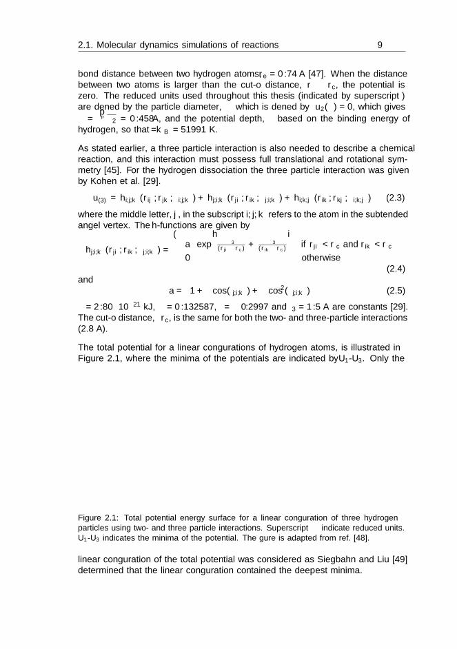
The total potential for a linear configurations of hydrogen atoms, is illustrated inFigure 2.1, where the minima of the potentials are indicated by U1-U3. Only the
Figure 2.1: Total potential energy surface for a linear configuration of three hydrogenparticles using two- and three particle interactions. Superscript ∗ indicate reduced units.U1-U3 indicates the minima of the potential. The figure is adapted from ref. [48].
linear configuration of the total potential was considered as Siegbahn and Liu [49]determined that the linear configuration contained the deepest minima.
10 Theoretical background
From the study in Chapter 4 it will be shown that the three-particle interaction leadto a large excluded volume diameter of the molecular fluid. This excluded volumediameter is in agreement with the Lennard-Jones diameter used by others [48].
2.1.2 Pressure calculations
The three-particle interaction potential will give a contribution to the overall pres-sure in the system [31,48]. From the virial theorem, the expression for the pressurein the presence of two- and three-particle interactions is:
P =kBTNpV
− 1
3V
Np∑
i=1
1
2
∑
j pair with i
∂u2(rij)
∂rijrij (2.6)
+∑
j<k triplet with i
(∂hi∂rji
rji +∂hi∂rik
rik +∂hi∂rjk
rjk
)
where pairs and triplets under the summation indicates that the summation isperformed over all pairs and triplets. The function hi is a function of the angle anddistances of a triplet formation.
hi = hj,i,k(rji, rik, θj,i,k) (2.7)
The first term in Eq. (2.6) gives the ideal contribution to the pressure due to thetotal number of particles, Np. The second and the third terms give the contributionsfrom the two- and three particle potentials, respectively. This makes it possible toquantify and compare the separate contributions to the pressure. The first studyof the three-particle interaction contribution to the overall pressure for a chemicalreaction was made by Xu et al. [30]. In Chapter 4 it will be shown that themagnitude of the three particle contribution to the pressure is dependent on thedegree of dissociation [48].
2.2 The Small System Method
In 1963 Hill [50] extended the range of the validity of the thermodynamic functionsand the mathematical interrelations between these functions to nonmacroscopicsystems, such as colloidal particles or one macroscopic molecule. In this situa-tions U, H and G are no longer extensive variables, and regular thermodynamicfunctions and relations are not valid. In 1998 Hill and Chamberlin [51–53] definednanothermodynamics to describe systems that are far from the thermodynamiclimit, i.e., systems with only a small number of particles. If the size of the smallsystem increases towards the size of an infinite system (Nj →∞ or Vj →∞), thethermodynamical equations for the small system becomes equal to the ordinarythermodynamical equations.
2.2. The Small System Method 11
The Small System Method is based on Hills formalism and the first reports of thiswas made by Schnell and coworkers [22–24] in 2011. This new method is underconstant development, with the latest extension to find partial molar enthalpies andreaction enthalpies, and the usage areas increases rapidly. This will be described indetail in Chapter 5, where also a more detailed description of the method is given.
2.2.1 Principles
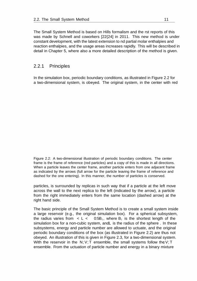
In the simulation box, periodic boundary conditions, as illustrated in Figure 2.2 fora two-dimensional system, is obeyed. The original system, in the center with red
Figure 2.2: A two-dimensional illustration of periodic boundary conditions. The centerframe is the frame of reference (red particles) and a copy of this is made in all directions.When a particle leaves the center frame, another particle enters from one adjacent frameas indicated by the arrows (full arrow for the particle leaving the frame of reference anddashed for the one entering). In this manner, the number of particles is conserved.
particles, is surrounded by replicas in such way that if a particle at the left moveacross the wall to the next replica to the left (indicated by the arrow), a particlefrom the right immediately enters from the same location (dashed arrow) at theright hand side.
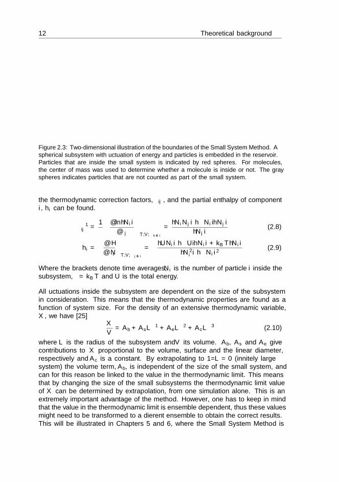
The basic principle of the Small System Method is to create a small system insidea large reservoir (e.g., the original simulation box). For a spherical subsystem,the radius varies from σ < L < 0.5Bi, where Bi is the shortest length of thesimulation box for a non-cubic system, and L is the radius of the sphere . In thesesubsystems, energy and particle number are allowed to fluctuate, and the originalperiodic boundary conditions of the box (as illustrated in Figure 2.2) are thus notobeyed. An illustration of this is given in Figure 2.3, for a two-dimensional system.With the reservoir in the N,V, T ensemble, the small systems follow the µ, V, Tensemble. From the fluctuation of particle number and energy in a binary mixture
12 Theoretical background
Figure 2.3: Two-dimensional illustration of the boundaries of the Small System Method. Aspherical subsystem with fluctuation of energy and particles is embedded in the reservoir.Particles that are inside the small system is indicated by red spheres. For molecules,the center of mass was used to determine whether a molecule is inside or not. The grayspheres indicates particles that are not counted as part of the small system.
the thermodynamic correction factors, Γij , and the partial enthalpy of componenti, hi can be found.
Γ−1ij =
1
β
(∂ ln〈Ni〉∂µj
)
T,V,µk 6=i
=〈NiNj〉 − 〈Ni〉〈Nj〉
〈Nj〉(2.8)
hi =
(∂H
∂Ni
)
T,V,µj 6=i
= −〈UNi〉 − 〈U〉〈Ni〉+ kBT 〈Ni〉〈N2
i 〉 − 〈Ni〉2(2.9)
Where the brackets denote time averages, Ni is the number of particle i inside thesubsystem, β = kBT and U is the total energy.
All fluctuations inside the subsystem are dependent on the size of the subsystemin consideration. This means that the thermodynamic properties are found as afunction of system size. For the density of an extensive thermodynamic variable,X, we have [25]
X
V= Ab +AsL
−1 +AeL−2 +AcL
−3 (2.10)
where L is the radius of the subsystem and V its volume. Ab, As and Ae givecontributions to X proportional to the volume, surface and the linear diameter,respectively and Ac is a constant. By extrapolating to 1/L = 0 (infinitely largesystem) the volume term, Ab, is independent of the size of the small system, andcan for this reason be linked to the value in the thermodynamic limit. This meansthat by changing the size of the small subsystems the thermodynamic limit valueof X can be determined by extrapolation, from one simulation alone. This is anextremely important advantage of the method. However, one has to keep in mindthat the value in the thermodynamic limit is ensemble dependent, thus these valuesmight need to be transformed to a different ensemble to obtain the correct results.This will be illustrated in Chapters 5 and 6, where the Small System Method is

2.3. Non-equilibrium thermodynamics 13
used to find partial enthalpies at constant T, V, µj and then transferred to partialmolar enthalpies (at T, P,Nj).
As the fluctuations inside the subsystem are size dependent, it is important to de-termine a region where size effects are negligible. This region, which is independentof the size of the reservoir, should be used when extrapolating to find the value inthe thermodynamic limit. As will be illustrated in Chapters 5 and 6 this regionis system dependent and has to be determined individually for each system. Thiscan be verified by running the same simulation with a larger simulation box (withthe same density).
2.2.2 Status of the Small System Method
Even though the Small System Method is fairly new (first reported in 2011), andcontinuously under extension, it has already proven to be useful for chemists. Liuet al. [54, 55] showed how this method could be used to find Fick diffusion coeffi-cients from Maxwell-Stefan diffusivities with the knowledge of the thermodynamiccorrection factors, which are found from particle fluctuations using the Small Sys-tem Method. In 2013, Schnell et al. [56] showed that the Small System Methodworks well for linearly dependent systems, such as the individual species in salt so-lution, which is an important property of this method compared to other simulationtechniques. The Small System Method was extended by Collell and Galliero [57]for in- homogeneous Lennard Jones fluids confined in slit pores to determine thethermodynamic factor of confined fluids. Recently, the method was used by Reif etal. [58] to calculate the thermodynamic correction factors for salt-water and salt-salt interactions. Trinh et al. [59] studied the adsorption of carbon dioxide on agraphite surface and thereby extended the Small System Method to surfaces. Thelatest extension, to calculate partial molar enthalpies and reaction enthalpies fromone single simulation, will be demonstrated in Chapter 5 [25]. In Chapter 6, themethod will be used to find reaction enthalpies and as a function of temperaturefor the dissociation of hydrogen, a system that is far from ideal conditions.
2.3 Non-equilibrium thermodynamics
Non-equilibrium thermodynamics is a useful tool to systematically describe trans-port processes, as it provides a theoretical description of transport properties forirreversible processes which are out of global equilibrium [12, 60]. Over the yearsseveral textbooks have been written on the subject, see e.g., references [12,60,61].The theory was established by Onsager in 1931 [62, 63] to describe transport pro-cesses in homogeneous systems. A systematic description of the extension to het-erogeneous systems, including transport into and through a surface was given byKjelstrup and Bedeaux in 2008 [12]. The two chapters that include non-equilibriumthermodynamics in the thesis both contain a chemical reaction, but in different
14 Theoretical background
ways. One reaction is present in the bulk phase (Chapter 7), the other at thesurface of a membrane (Chapter 3).
2.3.1 The entropy production of a chemically reacting sys-tem
The entropy production rate for a chemical reaction, e.g., H2 2H, with transportof heat and mass was given by Groot and Mazur [61], and this system will bediscussed in detail in Chapter 7.
σ = Jq∇(
1
T
)−∑
i
Ji∇µiT− r∆rG
T≥ 0 (2.11)
Here, Jq is the total heat flux, and Ji the molar component flux of either H or H2,with respect to the wall. ∇(1/T ) gives the temperature gradient in the x-,y- andz-direction, and ∇µi is the gradient in chemical potential of component i. r is thereaction rate, and ∆rG is the reaction Gibbs energy. The first two flux-force pairsare vectors, while the third flux-force pair, from the reaction, is a scalar, and doesfor this reason not couple to the other vectorial flux-force pairs. In the absence of anet mass flux through the system (JH = −2JH2), the rate of the reaction is definedas the gradient of the component flux
r = − ∂
∂xJH2
(x) =∂
∂x
1
2JH(x) (2.12)
The reaction Gibbs energy for the dissociative reaction is defined as
∆rG ≡ 2µH − µH2 (2.13)
The measurable heat flux, J ′q, is defined as
Jq = J ′q − JH2∆rH (2.14)
If only transport in the x-direction is considered, the entropy production rate ofthe reacting mixture can be rewritten
σ = J ′q∂
∂x
(1
T
)+
1
TJH2
∂
∂x(∆rG)T − r
∆rG
T(2.15)
Form the entropy production the following force-flux relations for transport of heatand mass [12] can be defined
d
dx
1
T= rqqJ
′q + rqµJH2 (2.16)
d
dx
∆rG
T= rµqJ
′q + rµµJH2 (2.17)
2.3. Non-equilibrium thermodynamics 15
where rii and rij are the main- and coupling coefficients, respectively, which de-scribes resistance to transport (here, heat and mass). The coupling coefficientsgives the possibility describe and quantify coupled transport, and are linked bythe Onsager reciprocal relations, rij = rji [62, 63]. For a chemically reactive sys-tem, the reaction rate can be regarded as a linear function of the driving forces if∆rG < RT [60]. In Chapter 7 a complete analytical procedure to describe chemicalreactions [26] is given. According to the definition by Onsager, the coefficients areonly dependent on state variables, such as temperature and density, and not onthe fluxes and forces. This means that a a temperature gradient can be used toincrease- or even to stop the mass flux. This will be discussed in detail in Chapter3, where transport of hydrogen through a palladium membrane will be studied.
The transport properties of the system, such as the diffusivity, thermal conductivityand heat of transfer etc., can all be found if the phenomenological coefficients areknown, this will be show in Chapters 3 and 7. However, these are not alwaysknown from experiments and often have to be estimated. This will be illustratedin Chapter 3, where it will be shown how non-equilibrium thermodynamics makesit possible to define experiments for finding both transport properties and thephenomenological coefficients.
With local chemical equilibrium, ∆rG = 0, the entropy production reduces to aone flux-force expression
σ = J ′q∂
∂x
(1
T
)(2.18)
2.3.2 Transport of a reacting mixture through a membrane
For transport of a mixture through a membrane, the entropy production (for oneside of the membrane) is given as
σm = Jmq∂
∂x
1
T+∑
j
Jmj∂
∂x
µjTm
(2.19)
where superscript m indicates the membrane. The force-flux relations for the mem-brane can be set up in a similar manner as described in the previous section. Inthe membrane, the enthalpy of the components is constant, and for this reason nocoupling effect of the heat- and mass flux is observed in the membrane, [12,64].
At the membrane surface, the situation is more complex. In non-equilibrium ther-modynamics, Gibbs definition of a dividing surface, “a geometrical plane, goingthrough points in the interfacial region, similarly situated with respect to to condi-tions of adjacent matter” [65], is used. With this definition, in terms of the excessdensities, the surface is treated as an autonomous thermodynamic system. Oneconsequence of this is that the surface has its own temperature, and that all itsproperties depend on this temperature alone, and not on the temperature of theadjacent phases. Consider a surface, s, separating two phases, i and o, as illustrated

16 Theoretical background
Figure 2.4: The density profile of a surface (shaded area), i and o indicate the adjacentphases. The excess surface density can be found by integration of the density profile. Thefigure has been reprinted and modified with permissions from the authors, ref. [12].
in Figure 2.4 for the excess surface density. With Gibbs definition of the excesssurface densities, normal thermodynamic relations, such as the first and secondlaws are valid [65]. The excess entropy production for a non-polarized surface inthe absence of an electric field has five independent flux-force pairs;
σs = J i,oq
(1
T s− 1
T i,o
)+ Jo,iq
(1
T o,i− 1
T s
)(2.20)
+
n∑
j=1
J i,oj
[−(µsjT s−µi,ojT i,o
)]+
n∑
j=1
Jo,ij
[−(µo,ijT o,i
−µsjT s
)]+ rs
(−∆nG
s
T s
)
for transport perpendicular to the surface. From the above equation, it can be seenthat coupling between −∆nG/T
s and ∆µ/T is now possible, unlike the situationin the bulk phase and the membrane. This will be examined in Chapter 3, whereit will also be shown that for transport of hydrogen across a palladium membrane,the entropy production reduces to two independent flux-force pairs.
Chapter 3
Assessing the coupled heatand mass transport ofhydrogen through apalladium membrane
Ragnhild Skorpa1, Mari Voldsund1, Marit Takla 1, SondreK. Schnell2, Dick Bedeaux1 and Signe Kjelstrup1,2
1. Department of Chemistry,Norwegian University of Science and Technology,
NO-7491 Trondheim, Norway
2. Process & Energy Laboratory,Delft University of Technology,
Leeghwaterstraat 39, 2628CB Delft,The Netherlands
This chapter was published inJ. Mem. Sci. (2012) 394–395:131–139
17

18Assessing the coupled heat and mass transport of hydrogen through a
palladium membrane
Abstract
We have formulated the coupled transport of heat and hydrogen through a palla-dium membrane, including the dissociative adsorption of hydrogen at the surface.This was done using the systematic approach of non-equilibrium thermodynamics.We show how this approach, which deviates from Sieverts’ law, makes is possibleto calculate the direct impact that a temperature gradient, or a heat flux, has onthe hydrogen flux. Vice versa, we show how the dissociative adsorption reactionleads to heat sinks and sources at the surface.
Using a set of transport coefficients estimated from experimental values availablein the literature, calculations were performed. An enhancement of the hydrogenflux through the membrane with 10% and 25%, by transmembrane temperaturedifferences of 24.8 K and 65.6 K, respectively, was predicted with a feed tempera-ture of 673 K. Similarly, a transmembrane temperature difference of −176.5 K wasobserved to stop the hydrogen flux (Soret equilibrium). The calculations are donewith estimated transport properties for the surfaces. The results show that aneffort should be put into determination of these. Such experiments are discussed.
3.1 Introduction
With increasing energy prices, and a limited supply of oil, it is of importance toimprove the efficiency of the most common industrial processes. In this situation,membrane reactors are interesting. In a membrane reactor, a chemical reactionand the separation of resulting products can be performed in one process step.The products are removed continuously along the reactor. This in situ removal ofthe products (or of unwanted by-products from the chemical reaction), as well asthe possibility of a high yield from equilibrium limited reactions, makes this a veryinteresting alternative to traditional reactors.
Membrane reactors can be put into two categories: porous and dense. Porousmembranes can be e.g. zeolite-based membranes [66,67], while the palladium mem-brane is a typical example of a dense membrane. In industrial applications, thereare several situations where one wishes to extract hydrogen from a reaction; thewater-gas-shift reaction [9] is one of the most important. For other examples, seeBasile [10]. The palladium membrane is a thin layer of palladium, often on a poroussupport of either steel or alumina. For a recent review of state of the art palladiummembrane reactors, see Yun and Oyama [11]. Palladium is purely selective towardstransport of H2. In order to give a high flux of hydrogen through the membrane,the palladium-layer should be as thin as possible; typically a few micro meter orless. In a palladium reactor hydrogen is transported as hydrogen atoms in thepalladium, and as hydrogen molecules in the gas phases on each side of the mem-brane [11, 68]. The heat of adsorption is significant (−87 kJ mol−1 [69]), includingthe splitting of molecular hydrogen and adsorption at the surface. This dissociative
3.1. Introduction 19
adsorption is likely to influence the mass flux. There is a need to study this in asystematic manner for several reasons. It is known that surface effects can hamperexperiments [70]. Also, permeability studies often show deviation from Sieverts’law [71]. Furthermore, while it is known how the absolute temperature affects achemical reaction, little is known on how a temperature gradient affects the reac-tion rate. With a thin membrane and large heat sinks and sources at the interfaces,such gradients may be large. The coupling of chemical reactions to fluxes of heatand mass is possible in principle [60], but has not been described in detail for areal system before.
In their now seminal paper, Ward and Dao [72], presented a model for hydrogenpermeation through a palladium membrane which accounted for all kinetic steps inthe permeation and reaction process. This model has been modified and improvedto also include mass transfer through the support by others, and has been furtherused a basis for incorporating the surface and a reaction in reactor models [73–77]. Many of the existing models for hydrogen permeation neglects the effect ofthe surface, see e.g [78, 79]. None of these works deal with transport of heat incombination with transport of mass across surfaces, however.
This gives us a motivation to apply non-equilibrium thermodynamics to study thetransport in a palladium membrane. The work of de Groot and Mazur [61] outlineshow to describe homogeneous systems. During the last decade, the field has beenfurther developed to also include heterogeneous systems, such as systems withmembranes [12]. In the extension, dynamic boundary conditions for the crossingfrom one layer to the next were defined. The coupling, or the interaction of fluxesand forces at the surface, is often overlooked in the literature, while it is now knownthat it can be substantial [80]. It is, however, relevant to ask whether linear force-flux relations apply when a chemical reaction takes place in the system. Chemicalreactions have normally rates which are non-linear functions of their driving force,meaning that we then need to go to a mesoscopic level of description to capturethis property [60]. In the present case, we shall see that there is no need to invokethis level of complication for operating conditions that are typical for palladiumtransport.
After a short description of the system and the system conditions used in Section3.2, we proceed in Section 3.3 to derive transport equations, using non-equilibriumthermodynamics, across a palladium membrane. Details concerning the calcula-tions and solution procedures are given in Section 3.4. In Section 3.5 we presentand discuss the results obtained from applying the model to different sets of bound-ary conditions. We study in particular the effect the surface has on the transportacross the membrane. In Section 3.6, we draw conclusions.
20Assessing the coupled heat and mass transport of hydrogen through a
palladium membrane
3.2 The system
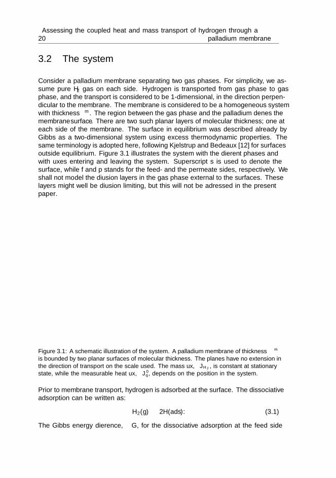
Consider a palladium membrane separating two gas phases. For simplicity, we as-sume pure H2 gas on each side. Hydrogen is transported from gas phase to gasphase, and the transport is considered to be 1-dimensional, in the direction perpen-dicular to the membrane. The membrane is considered to be a homogeneous systemwith thickness δm. The region between the gas phase and the palladium defines themembrane surface. There are two such planar layers of molecular thickness; one ateach side of the membrane. The surface in equilibrium was described already byGibbs as a two-dimensional system using excess thermodynamic properties. Thesame terminology is adopted here, following Kjelstrup and Bedeaux [12] for surfacesoutside equilibrium. Figure 3.1 illustrates the system with the different phases andwith fluxes entering and leaving the system. Superscript s is used to denote thesurface, while f and p stands for the feed- and the permeate sides, respectively. Weshall not model the diffusion layers in the gas phase external to the surfaces. Theselayers might well be diffusion limiting, but this will not be adressed in the presentpaper.
Figure 3.1: A schematic illustration of the system. A palladium membrane of thickness δm
is bounded by two planar surfaces of molecular thickness. The planes have no extension inthe direction of transport on the scale used. The mass flux, JH2 , is constant at stationarystate, while the measurable heat flux, J ′q, depends on the position in the system.
Prior to membrane transport, hydrogen is adsorbed at the surface. The dissociativeadsorption can be written as:
H2(g) 2H(ads). (3.1)
The Gibbs energy difference, ∆G, for the dissociative adsorption at the feed side

3.3. A thermodynamic description of transport 21
can then be defined as∆G = 2µm
H − µfH2, (3.2)
where µij is the chemical potential of component j in phase i evaluated close to the
surface (here surface at the feed side). As only equations for the feed side of themembrane is given in detail in this paper, the superscripts indicating the phase (f,m or p) have been dropt for ∆G throughout the paper. For the permeate side, asimilar expression as given in Eq.(3.2) can be obtained.
We shall study the stationary state, where there is no accumulation of mass any-where in the system, and
rs =1
2JH = JH2
. (3.3)
Here rs is the rate of the dissociative adsorption, JH is the flux of atomic hydrogenthrough the membrane, and JH2 is the rate of which H2 enters and leaves thesystem per m2.
The total heat flux, Jq, through the system is also constant in the stationary state,giving
Jq = J ′fq + JH2H f
H2= J ′mq + JHH
mH = J ′pq + JH2
HpH2, (3.4)
which rearranged gives
J ′fq = J ′mq + ∆HJH2= J ′pq , (3.5)
where H ij is the enthalpy of component j in phase i, ∆H = 2Hm
H − H fH2
= 2HmH − Hp
H2is the heat of dissociative adsorption and J ′iq is the measurable
heat flux in phase i. Constant enthalpy in each phase was assumed.
3.3 A thermodynamic description of transport
In Sections 3.3.1 (for the membrane) and 3.3.2 (for the surface) we present theentropy production for each subsystem. The entropy production determines therelevant forces and fluxes, and their interactions. For details in the derivationwe refer to the literature [12]. All the presented equations are given for the feedside of the membrane and for the surface at the feed side only. Equations for thepermeate side are analogous and can be found in a similar manner. The force-flux relationships defines the necessary and sufficient experiments for determiningtransport coefficients. We shall further make a link to the experimental data wetake from the literature.
3.3.1 The membrane
The general expression for entropy production in a homogeneous phase is definedas the linear combination of fluxes and forces, and is described in several texts
22Assessing the coupled heat and mass transport of hydrogen through a
palladium membrane
on non-equilibrium thermodynamics, see e.g. [12, 61]. For transport of heat andatomic hydrogen in the membrane, we have the following expression, choosing therepresentation with the measurable heat flux, J ′mq
σm = J ′mq∂
∂x
(1
T
)+ Jm
H
(− 1
Tm
∂µH,T
∂x
). (3.6)
Here, JH is the flux of atomic hydrogen, while ∂µH,T /∂x is the gradient in chemicalpotential for atomic hydrogen at a constant temperature, Tm. The derivation isshown for the corresponding processes across the surface in 3.B. The expressionmeans, that dissipative processes at stationary state are connceted to heat transportand transport of atomic hydrogen.
We express the flux of atomic hydrogen from the surface through the membranewith the flux of molecular hydrogen outside the membrane, JH2 , using Eq.(3.3). Wesee that taking the measurable heat flux constant across the membrane simplifiesthe integration. We find that it results in a calculation error of less than 2% forthe entropy balance. For the whole membrane, we obtain the entropy productionper surface area
σmδm = J ′mq ∆m
(1
T
)+ JH2
(− 2
Tm∆mµH,T
), (3.7)
where ∆m means the difference between the right and left hand side in the mem-brane phase. The force-flux relations for the membrane phase are
∆m
(1
T
)= rm
qqJ′mq + rm
qµJH2 , (3.8)
− 2
T(∆mµH,T ) = rm
µqJ′mq + rm
µµJH2 , (3.9)
where rii and rij are the main- and cross coefficients, respectively, which describeresistance to transport. The cross coefficients describe coupling between the differ-ent fluxes, here the mass- and heat flux, and are linked by the Onsager reciprocalrelations, rij = rji [62,63].
In order to solve Eqs.(3.8) and (3.9), we need values for the main- and cross coef-ficients. Only three coefficients are independent, given the validity of the Onsagerrelations. The first coefficient, rm
qq, can be found from the membrane thermal con-ductivity, λm, which is defined at zero mass flux
λm = −[
J ′mq∆mT/δm
]
JH2=0
=1
T 2rmqq
. (3.10)
The second coefficient, the coupling coefficient, can best be found via the measur-able heat of transfer in the membrane, q∗mH . This property is defined as the ratio
3.3. A thermodynamic description of transport 23
between the measurable heat flux and mass flux at zero temperature gradient [12]
q∗mH =
(J ′mqJH2
)
∆mT=0
= −rmqµ
rmqq
. (3.11)
From Eq.(3.11) the measurable heat of transfer is also equal to the negative ratiobetween the cross coefficient and the resistivity of the heat flux.
The coupling coefficient makes it possible to describe mass transport that takesplace due to a temperature gradient, the Soret effect. The Soret effect is describedby the Soret cefficient, sT , which is defined according to [12] for a system in sta-tionary state as
sT = −(∂cH2
/∂x
cH2∂T/∂x
)
JH2=0
=q∗mH
cH2
(∂µH2,T
∂cH2
)−1
, (3.12)
where cH2is the concentration of molecular hydrogen. This means that a temper-
ature gradient in principle can be used to stop the mass flux. We define such acondition as the Soret equilibrium. This condition can be used to experimentallydetermine the coupling coefficient.
The third independent coefficient is the mass transfer resistance rmµµ. It is now
common to report the membrane permeability, Πm, of molecular hydrogen usingSieverts’ law for the isothermal interface
JH2|∆T=0 = −Πm
((pp
H2
)0.5 −(pf
H2
)0.5
δm
). (3.13)
Here piH2
is the partial pressure of hydrogen in the bulk gas phase i (feed or per-meate). We specify in 3.A the conditions for which this equation is valid.
The expression in Eq.(3.13) can be used to find rmµµ from Πm, by neglecting any
pressure gradient in the diffusion layer next to the surface. At isothermal conditionsand with chemical equilibrium at the surfaces, the force-flux equations, Eqs.(3.8)and (3.9), reducees to
JH2 |∆T=0 = −2R
δmln
(pp
H2
pfH2
)0.5(rmµµ −
rmqµr
mµq
rmqq
)−1
, (3.14)
where R is the universal gas constant. We have used the definition of the chemical
potential, µH = µ0H + RT ln aH, where aH = K
(pH2
/p0)0.5
(cf. 3.A), p0=1 baris the standard state pressure and K is the equilibrium constant for the reactiongiven in (3.1).
When these conditions apply, we find rmµµ from Πm, setting Eqs.(3.13) and (3.14)
equal, knowing rmqq (λm) and rm
qµ (q∗,m). The result is:
rmµµ =
(q∗,m)2
T 2λm−
R ln
(ppH2
pfH2
)
Πm((pf
H2
)0.5 −(pp
H2
)0.5) . (3.15)

24Assessing the coupled heat and mass transport of hydrogen through a
palladium membrane
The result can be used under arbitrary conditions, as the transport coefficientsdo not depend on the forces or the fluxes, according to the basic postulates ofnon-equilibrium thermodynamics.
3.3.2 The surfaces
The excess entropy production of the surface, has in the outset five independentconjugate flux-force pairs for transport of heat and mass in the presence of a surfacereaction, see Kjelstrup and Bedeaux [12]. We show in 3.B, how the five pairs canbe reduced to two at stationary state conditions. For the surface at the feed side,we obtain:
σs = J ′fq ∆f,m
(1
T
)+ JH2
[− 1
Tm∆G(Tm)
], (3.16)
where J ′fq is the measurable heat flux. Gibbs energy difference, ∆G, was definedin Eq.(3.2), and ∆G(Tm) means that it is evaluated at the temperature in themembrane close to the surface at the feed side.
The resulting force-flux relations for the surface at the feed side are then
∆f,m
(1
T
)= rs
qqJ′fq + rs
qµJH2, (3.17)
− 1
Tm∆G(Tm) = rs
µqJ′fq + rs
µµJH2. (3.18)
The surface excess resistivities have the dimensionality of membrane resistivitiestimes a length. They can be found in a similar manner as shown for the membrane.
For the right-hand side surface, the excess entropy production can be derived in ananalogous manner as illustrated for the left-hand side surface in 3.A. The resultingexpression is similar. The force-flux relations follow from this in a similar manneras shown for the other surface.
3.4 Calculation details
3.4.1 Determination of resistivities
The resistivities for the membrane and the surfaces were calculated using the rela-tions described in Section 3.3 and data from the literature given in Table 3.1. Theresulting resistivities are given in Table 3.2.
Each set of coefficients (in phase i) was tested for consistency with the second lawof thermodynamics using [12]
Di = riµµr
iqq − ri
µqriqµ ≥ 0. (3.19)
3.4. Calculation details 25
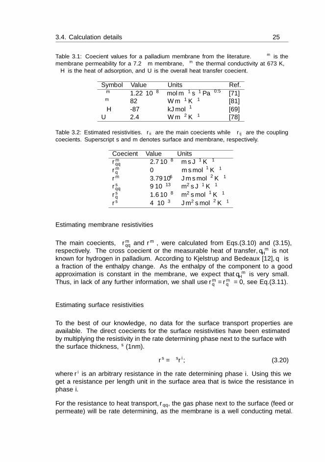
Table 3.1: Coefficient values for a palladium membrane from the literature. Πm is themembrane permeability for a 7.2 µm membrane, λm the thermal conductivity at 673 K,∆H is the heat of adsorption, and U is the overall heat transfer coefficient.
Symbol Value Units Ref.
Πm 1.22 ·10−8 mol m−1 s−1 Pa−0.5 [71]λm 82 W m−1 K−1 [81]
∆H -87 kJ mol−1 [69]U 2.4 W m−2 K−1 [78]
Table 3.2: Estimated resistivities. rii are the main coefficients while rij are the couplingcoefficients. Superscript s and m denotes surface and membrane, respectively.
Coefficient Value Unitsrmqq 2.7·10−8 m s J−1 K−1
rmqµ 0 m s mol−1 K−1
rmµµ 3.79·106 J m s mol−2 K−1
rsqq 9·10−13 m2 s J−1 K−1
rsqµ 1.6·10−8 m2 s mol−1 K−1
rsµµ 4· 10−3 J m2 s mol−2 K−1
Estimating membrane resistivities
The main coefficients, rmqq and rm
µµ, were calculated from Eqs.(3.10) and (3.15),respectively. The cross coefficient or the measurable heat of transfer, q∗mH is notknown for hydrogen in palladium. According to Kjelstrup and Bedeaux [12], q∗ isa fraction of the enthalpy change. As the enthalpy of the component to a goodapproximation is constant in the membrane, we expect that q∗mH is very small.Thus, in lack of any further information, we shall use rm
µq=rmqµ = 0, see Eq.(3.11).
Estimating surface resistivities
To the best of our knowledge, no data for the surface transport properties areavailable. The direct coefficients for the surface resistivities have been estimatedby multiplying the resistivity in the rate determining phase next to the surface withthe surface thickness, δs (1nm).
rs = δsri, (3.20)
where ri is an arbitrary resistance in the rate determining phase i. Using this weget a resistance per length unit in the surface area that is twice the resistance inphase i.
For the resistance to heat transport, rqq, the gas phase next to the surface (feed orpermeate) will be rate determining, as the membrane is a well conducting metal.
26Assessing the coupled heat and mass transport of hydrogen through a
palladium membrane
Thus, we used the overall heat transfer coefficient, U , given for a similar systemby Johannessen and Jordal [78], to determine the thermal conductivity in the gasphase, λg. The resistance in the membrane is neglected.
λg = Uδtot. (3.21)
Here δtot is the total thickness of the system (1 mm) from bulk to bulk phase. δtot
was used as an estimate for the thickness of the gas phase, as the membrane underinvestigation is thin (δm = 7.2µm).
δg = δtot − δm − 2δs ' δtot. (3.22)
The resistance to heat transfer in the gas phase, rgqq, was then calculated analogous
to the relation given in Eq.(3.11). When this was known, it was possible to estimatersqq from rg
qq according to Eq. (3.20).
The rate determining layer for resistance to mass transfer, is the membrane. Hence,rsµµ was then estimated from rm
µµ according to Eq. (3.20).
According to Kjelstrup and Bedeaux [12], the heat of transfer, q∗, for the wholesurface, defined analogous as in Eq.(3.11), can also be written as
q∗s = −k∆H, (3.23)
(cf. Eq.(11.24) in [12]). Thus, q∗s can be expressed as a fraction, k, of the enthalpychange over the interface. Kinetic theory predicts that k = 0.2, see [12]. In lack ofbetter information, we have used the kinetic theory-value also in this case.
It is known that the surface has a high resistivity, thus we shall increase the valueof the set of coefficients by a factor α = 10 or 100. The set with α = 10 shall becalled the basis set.
A major difference between the transport properties of the surface and the homoge-neous phases is that the coupling coefficients can be neglected in the homogeneousphase, but not at the surface, due to surface properties described above. In thestate-of-the art description the coupling coefficients are neglected also at the sur-face, and we shall examine the effect of this assumption.
3.4.2 Investigated cases
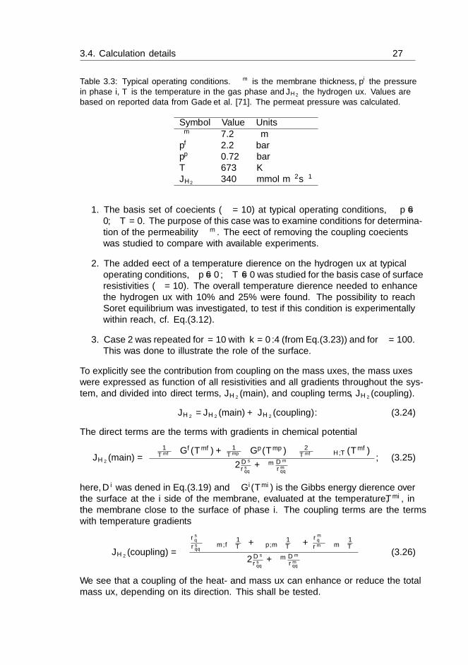
In order to investigate the effect of coupling and thermal driving forces on themembrane performance, we started with a typical set of operating conditions, de-termined from reported values by Gade et al. [71] for a 7.2 µm thick membrane.The pressure at the permeate side was calculated based on values in [71]. Thevalues are given in Table 3.3.
The following cases were studied:
3.4. Calculation details 27
Table 3.3: Typical operating conditions. δm is the membrane thickness, pi the pressurein phase i, T is the temperature in the gas phase and JH2 the hydrogen flux. Values arebased on reported data from Gade et al. [71]. The permeat pressure was calculated.
Symbol Value Unitsδm 7.2 µmpf 2.2 barpp 0.72 barT 673 KJH2
340 mmol m−2s−1
1. The basis set of coefficients (α = 10) at typical operating conditions, ∆p 6=0,∆T = 0. The purpose of this case was to examine conditions for determina-tion of the permeability Πm. The effect of removing the coupling coefficientswas studied to compare with available experiments.
2. The added effect of a temperature difference on the hydrogen flux at typicaloperating conditions, ∆p 6= 0,∆T 6= 0 was studied for the basis case of surfaceresistivities (α = 10). The overall temperature difference needed to enhancethe hydrogen flux with 10% and 25% were found. The possibility to reachSoret equilibrium was investigated, to test if this condition is experimentallywithin reach, cf. Eq.(3.12).
3. Case 2 was repeated for α = 10 with k = 0.4 (from Eq.(3.23)) and for α = 100.This was done to illustrate the role of the surface.
To explicitly see the contribution from coupling on the mass fluxes, the mass fluxeswere expressed as function of all resistivities and all gradients throughout the sys-tem, and divided into direct terms, JH2
(main), and coupling terms, JH2(coupling).
JH2=JH2
(main) + JH2(coupling). (3.24)
The direct terms are the terms with gradients in chemical potential
JH2(main) =− 1Tmf ∆Gf(Tmf) + 1
Tmp ∆Gp(Tmp)− 2Tmf
(∆µH,T (Tmf)
)
2Ds
rsqq+ δmDm
rmqq
, (3.25)
here, Di was defined in Eq.(3.19) and ∆Gi(Tmi) is the Gibbs energy difference overthe surface at the i side of the membrane, evaluated at the temperature, Tmi, inthe membrane close to the surface of phase i. The coupling terms are the termswith temperature gradients
JH2(coupling) = −rsµqrsqq
(∆m,f
(1T
)+ ∆p,m
(1T
))+
rmµqrmµµ
∆m
(1T
)
2Ds
rsqq+ δmDm
rmqq
(3.26)
We see that a coupling of the heat- and mass flux can enhance or reduce the totalmass flux, depending on its direction. This shall be tested.
28Assessing the coupled heat and mass transport of hydrogen through a
palladium membrane
3.4.3 Solution procedure
We have two transport equations for each layer; one for heat and one for mass.Eqs.(3.8) and (3.9) describe the transport in the membrane. The transport at thefeed side of the surface is described by Eqs.(3.17) and (3.18), and we have similarequations for the other surface. Altogether we have six transport equations for thewhole system. As we have stationary state conditions, we also have the relationgiven in Eq.(3.5).
With constant resistivities and constant enthalpies in each phase and known con-ditions at the gas side, the above equations were integrated across each layer, andsolved for JH2
, J ′fq and temperature and hydrogen activity in the membrane closeto the surface at each side. This was done numerically.
3.5 Results and discussion
3.5.1 Operating conditions for permability studies with thebasis set of coefficients
Permeability experiments are normally done with relatively small pressure differ-ences and for isothermal conditions. Under such conditions one may expect thatSieverts’ law applies, cf. 3.A. In case 1, we examined the local conditions fortransport, for experiments where T f = T p.
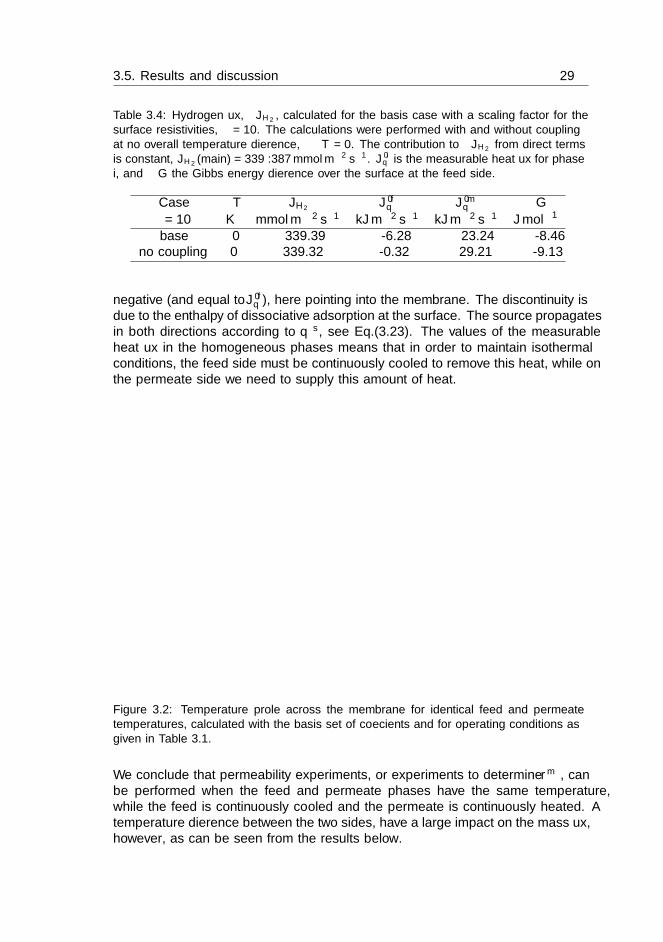
The temperature profile across the membrane was first calculated with the basis setof resistivity coefficients (α = 10). The result is shown in Figure 3.2 and Table 3.4,for the operating conditions given in Table 3.1. The profile is antisymmetric aroundthe plane through the membrane center, as expected from the heat source we haveon the left and the heat sink on the right-hand side. The temperature jumps atthe surfaces are, however, insignificant in magnitude, meaning that the membranein practice is isothermal, as assumed in Eq.(3.14). Experiments with ∆T = 0should thus give resonable values for Πm. The same applies to the jumps in thechemical potential. The ∆G at the surface was observed to be -8.46 J mol−1 and-9.13 J mol−1 with and without coupling, respectively. The assumption of chemicalequilibrium at the surface is thus approximately valid for this set of coefficients.The corresponding hydrogen flux is therefore also not altered by including coupling,as can be seen from Table 3.4.
In spite of the seemingly small effects from coupling on the temperature profiles,it is interesting to note that the heat flux vary largely between the membraneand its surroundings. The measurable heat flux in the membrane is positive andlarge, 23 kJ mol−1, while on the feed side it is -6.3 kJ mol−1, meaning that heat istransported into the feed side. The measurable heat flux on the permeate side is also
3.5. Results and discussion 29
Table 3.4: Hydrogen flux, JH2 , calculated for the basis case with a scaling factor for thesurface resistivities, α = 10. The calculations were performed with and without couplingat no overall temperature difference, ∆T = 0. The contribution to JH2 from direct termsis constant, JH2(main) = 339.387 mmol m−2 s−1. J ′iq is the measurable heat flux for phasei, and ∆G the Gibbs energy difference over the surface at the feed side.
Case ∆T JH2J ′fq J ′mq ∆G
α = 10 K mmol m−2 s−1 kJ m−2 s−1 kJ m−2 s−1 J mol−1
base 0 339.39 -6.28 23.24 -8.46no coupling 0 339.32 -0.32 29.21 -9.13
negative (and equal to J ′fq ), here pointing into the membrane. The discontinuity isdue to the enthalpy of dissociative adsorption at the surface. The source propagatesin both directions according to q∗s, see Eq.(3.23). The values of the measurableheat flux in the homogeneous phases means that in order to maintain isothermalconditions, the feed side must be continuously cooled to remove this heat, while onthe permeate side we need to supply this amount of heat.
Feed Membrane Permeate−1.5
−1.0
−0.5
0.0
0.5
1.0
1.5
Tem
per
atu
re,
[K]
×10−3
673.0 K 673.0 K
No Coupling
Coupling
Figure 3.2: Temperature profile across the membrane for identical feed and permeatetemperatures, calculated with the basis set of coefficients and for operating conditions asgiven in Table 3.1.
We conclude that permeability experiments, or experiments to determine rmµµ, can
be performed when the feed and permeate phases have the same temperature,while the feed is continuously cooled and the permeate is continuously heated. Atemperature difference between the two sides, have a large impact on the mass flux,however, as can be seen from the results below.
30Assessing the coupled heat and mass transport of hydrogen through a
palladium membrane
3.5.2 Non-isothermal operating conditions with the basis setof coefficients
Using the basis set of coefficients (α = 10), we calculated temperature differencesrequired to enhance the mass flux by 10% and 25%, and the temperature differencerequired to stop the hydrogen flux (Soret equilibrium, Eq.(3.12)). The results aregiven in Table 3.5. From Table 3.5 we see that a positive temperature differencewill enhance the mass flux, while a negative temperature difference is requiredto obtain Soret equilibrium. A positive temperature difference implies that thetemperature shall be higher at the permeate side than at the feed side. Accordingto Le Chatelier’s principle, increasing the temperature at the permeate side shiftsthe endothermic desorption reaction towards the product. In the same way, theexothermic adsorption reaction will be shifted towards products by lowering thetemperature at the feed side. This facilitates the formation of H in the membraneat the feed side, and the formation of H2 at the permeate side, thereby increasingJH2 .
Table 3.5: Hydrogen flux, JH2 , and overall temperature difference, ∆T , calculated forscenarios with mass flux increased by 10% and 25% and Soret equilibrium (zero massflux). J ′iq is the measurable heat flux in phase i, and ∆G is Gibbs energy difference overthe surface at the feed side. For the basis case, the surface resistivities are multiplied witha factor, α = 10. The contribution to JH2 from direct terms is constant, JH2(main) =339 mmol m−2 s−1.
Case ∆T JH2J ′fq J ′mq ∆G
α = 10 K mmol m−2 s−1 kJ m−2 s−1 kJ m−2 s−1 J mol−1
+10% 24.8 373 -2909 -2877 308+25% 65.6 424 -7264 -7227 806Soret -176.5 0 29021 29021 -2657
It was observed that a temperature difference of -176 K was needed to stop thehydrogen flux (Soret equilibrium), cf. Table 3.5. From the table we observe thatwhen JH2
= 0, J ′fq = J ′mq = J ′pq = Jq (cf. Eqs.(3.4) and (3.5)). This situation maybe achieved in the laboratory, and can then be used to find the coupling coefficient,which is the direct cause of this effect.
A plot of JH2and JH2
(main) versus temperature difference is given in Figure 5.4.From the figure we see that the fraction of the flux caused by direct terms (JH2
(main))is constant in spite of temperature changes in the system. Variation with tempera-ture is seen for the total flux, and is thus caused by coupling terms (cf. Eq.(3.24)).Thus, application of a temperature gradient gives a significant contribution to theoverall mass transfer across the membrane.
The reaction Gibbs energy difference was observed to be smaller than RT in allscenarios (see Table 3.5). This means that the reaction rate can be regarded as alinear function of the driving force [60], justifying that the linear version of non-equilibrium thermodynamics is sufficient for a good description. It was observed
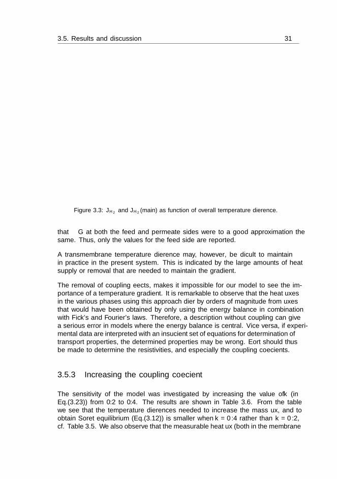
3.5. Results and discussion 31
−2.0 −1.5 −1.0 −0.5 0.0 0.5 1.0∆T [K] ×102
0
1
2
3
4
5
Mas
sF
lux
[mmol/m
2s]
×102
JH2(total)
JH2(main)
Figure 3.3: JH2 and JH2(main) as function of overall temperature difference.
that ∆G at both the feed and permeate sides were to a good approximation thesame. Thus, only the values for the feed side are reported.
A transmembrane temperature difference may, however, be difficult to maintainin practice in the present system. This is indicated by the large amounts of heatsupply or removal that are needed to maintain the gradient.
The removal of coupling effects, makes it impossible for our model to see the im-portance of a temperature gradient. It is remarkable to observe that the heat fluxesin the various phases using this approach differ by orders of magnitude from fluxesthat would have been obtained by only using the energy balance in combinationwith Fick’s and Fourier’s laws. Therefore, a description without coupling can givea serious error in models where the energy balance is central. Vice versa, if experi-mental data are interpreted with an insufficient set of equations for determination oftransport properties, the determined properties may be wrong. Effort should thusbe made to determine the resistivities, and especially the coupling coefficients.
3.5.3 Increasing the coupling coefficient
The sensitivity of the model was investigated by increasing the value of k (inEq.(3.23)) from 0.2 to 0.4. The results are shown in Table 3.6. From the tablewe see that the temperature differences needed to increase the mass flux, and toobtain Soret equilibrium (Eq.(3.12)) is smaller when k = 0.4 rather than k = 0.2,cf. Table 3.5. We also observe that the measurable heat flux (both in the membrane

32Assessing the coupled heat and mass transport of hydrogen through a
palladium membrane
Table 3.6: Hydrogen flux, JH2 , and overall temperature difference, ∆T , calculated forscenarios with mass flux increased by 10% and 25% and Soret equilibrium (zero massflux). The basis case for the surface resistivities where used, but the coupling coefficientwere doubled. J ′iq is the measurable heat flux in phase i and ∆G the reaction Gibbs energydifference at the feed side of the surface. The contribution to JH2 from direct terms isconstant, JH2(main) = 339.599 mmol m−2 s−1.
Case ∆T JH2J ′fq J ′mq ∆G
α = 10, k = 0.4 K mmol m−2 s−1 kJ m−2 s−1 kJ m−2 s−1 J mol−1
base 0 339.60 -12.26 17.28 -6.50no coupling 0 339.32 -0.32 29.21 -9.13
+10% 12.2 374 -1464 -1432 308+25% 31.3 425 -3645 -3608 791Soret -101.5 0 14513 14513 -2873
and in the feed) is smaller along with an observed decrease in ∆G, compared toTable 3.5. This is expected, as a larger coupling at the surface will enhance thesurface effects.
3.5.4 Increasing the resistivities
We also studied the effect of increasing the resistivities from the basis set withα = 10 to a set with α = 100. The results are given in Table 3.7.
Table 3.7: Hydrogen flux, JH2 , and overall temperature difference, ∆T , calculated forscenarios with mass flux increased by 10% and 25% and Soret equilibrium (zero massflux). J ′iq is the measureable heat flux in phase i and ∆G the reaction Gibbs energydifference at the feed side of the surface. The surface resistivities are multiplied with afactor, α = 100. The contribution to JH2 from direct terms is constant, JH2(main) =331.290 mmol m−2 s−1.
Case ∆T JH2 J ′fq J ′mq ∆G
α = 100 K mmol m−2 s−1 kJ m−2 s−1 kJ m−2 s−1 J mol−1
+10% 24.6 364 -297 -266 226+25% 64.9 414 -733 -697 709Soret -175.2 0 2902 2902 -2658
We observe a small difference for the mass flux between two sets of surface resistivi-ties (α = 10 and α = 100) by comparing Tables 3.5 and 3.7. Thus, when looking atthe mass flux, the overall picture is not much changed. The observed temperaturejumps (∆T ) become smaller along with a smaller contribution from coupling. Theeffect was, however, not proportional to the change in surface resistivities. For J ′iqthe observed effect was proportional to the change in surface resistivities (a de-crease by a factor ten was observed compared to Table 3.5). A decrease was alsoobserved for ∆G.
3.6. Conclusion 33
3.6 Conclusion
We have modelled transport of hydrogen through a palladium membrane usingthe framework of non-equilibrium thermodynamics. The model gives a systematicapproach to quantify surface effects, in particular the thermal effects associatedwith transport, but also of the dissociative adsorption at the surface.
The calculations were based on estimated resistivities, and given that these are re-alistic, we have found that the chemical reaction is most likely described by a linearflux-force regime. We also found that a transmembrane temperature difference canobstruct the validity of Sieverts’ law.
Our calculations predict that heating at the permeate side will increase the flux ofhydrogen. The overall temperature difference needed for enhancing the mass fluxwith 10% and 25%, for the basis case, was found to be 27.3 K and 72.5 K, respec-tively, with an initial feed temperature of 673 K. Similarly, an overall temperaturedifference of −176.5 K will stop the hydrogen flux. Thus, cooling the permeate sidegives a negative temperature gradient and a decrease in the mass flux.
When the scaling factor for the surface resistivities were changed from α = 10to α = 100, a small decrease was seeen for the overall temperaure differences.Only increasing the coupling coefficient (α = 10, k = 0.4), however, lead to largerchanges in the observed overall temperature difference.
As the results depend on the estimated resistivities, effort should be put into amore exact determination of these, to bring this work further. The coupling co-efficient leading to Soret equilibrium, is unknown for the surfaces as well as forthe membrane transport of hydrogen. The surface main resistivies to mass andheat transfer are also not known, and needs to be determined for a more exactdescription of the system.
Acknowledgments
SKS and SK acknowledge financial support from NWO-CW through an ECHOgrant, and computational resources were sponsored by the Stichting NationaleComputerfaciliteiten (National Computing Facilities Foundation, NCF), with fi-nancial support from the Nederlandse Organisatie voor Wetenschappelijk onder-zoek (Netherlands Organization for Scientific Research, NWO).
34Assessing the coupled heat and mass transport of hydrogen through a
palladium membrane
3.A Conditions for application of Sieverts’ law
Sieverts’ law gives the equilibrium concentration for atomic hydrogen, cH, in themetal [82] as:
cH = K(ppH2
)0.5 (3.27)
Here, ppH2
is the partial pressure of molecular hydrogen at the permeate side, and K
is the equilibrium constant for reaction (3.1). As p0H2
= 1bar, it has been removedfrom the equality and the rest of the appendix.
When this relation (Eq. (3.27)) is introduced into Fick’s law (the first equalitybelow), we find the equation commonly used to describe hydrogen permeability inmembranes:
JH2|∆T=0 = −Dm
H
(cpH − cfHδm
)
= −DmHK
((pp
H2
)0.5 −(pf
H2
)0.5
δm
)
= −Πm
((pp
H2
)0.5 −(pf
H2
)0.5
δm
). (3.28)
Here JH2is the flux of molecular hydrogen, Dm
H is the diffusion constant for atomichydrogen in palladium, δm is the thickness of the membrane, Πm is the membranepermeability of atomic hydrogen, pH2
is the partial pressure of hydrogen in thehomogeneous phases (feed or permeate). Some authors also denote this equationas Sieverts’ law. We shall specify the conditions for which the equation is valid.
At chemical equilibrium, the chemical potential differences for adsorption and re-action over the surface obey
∆G = 2µmH − µf
H2, (3.29)
where ∆G is the Gibbs energy difference for the dissociative adsorption at thesurface.
The chemical potential for molecular hydrogen in the gas phase, µfH2
, assumingideal gas, is
µfH2
= µ0,fH2
+RT ln pH2 , (3.30)
where µ0,ij is the chemical potential at standard state conditions for component j
in phase i. The chemical potential for atomic hydrogen adsorbed at the membranesurface is defined by
µmH = µ0,m
H +RT ln aH, (3.31)
where aH is the activity of hydrogen on the surface.

3.B. The entropy production for a palladium surface with hydrogen 35
By introducing Eqs.(3.30) and (3.31) for the chemical potentials into Eq.(3.2), andwith ∆G = 0, we obtain for the feed side
2µ0,mH − µ0,f
H2= RT ln
a2H
pH2
= ∆G0. (3.32)
Here ∆G0 is the standard state Gibbs energy.
We rearrange and obtain the following expression for the activity of atomic hydro-gen near the membrane surface at equilibrium conditions
aH =
[exp
(∆G0
RT
)]0.5
p0.5H2
= Kp0.5H2. (3.33)
The activity of atomic hydrogen at the surface is further defined by
aH = cHγ, (3.34)
where cH is the concentration of atomic hydrogen near the surface and γ is theactivity coefficient. For an ideal surface γ = 1. For Langmuir adsorption, γ =1/(1− θ) where θ is the surface coverage [83]. With γ equal unity or constant, wehave
cH = K ′p0.5H2, (3.35)
where K ′ is the equilibrium constant divided by the activity coefficient. For lowcoverage it is the equilibrium constant, and Eq.(3.35) is reduced to Eq.(3.27) (Siev-erts’ law [82]).
Experimental results give often values for the exponent that deviates from 0.5 [71].We have seen that Eq.(3.28) can be expected to hold, when there is equilibrium foradsorption and reaction in the surface, when the conditions are isothermal, whenthe hydrogen gas is ideal, and when the surface activity coefficient is unity (thecoverage is small or nearly constant).
3.B The entropy production for a palladium sur-face with hydrogen
We are interested in the excess entropy production, σs, for hydrogen and heattransport through a palladium surface, and start with the general expression de-rived by Kjelstrup and Bedeaux [12]. For a non-polarized surface, in the absenceof an electric current, we have
σs = J iq
(1
T s− 1
T i
)+ Jo
q
(1
Tm− 1
T s
)+
n∑
j=1
J ij
[−(µsj
T s−µij
T i
)]
+
n∑
j=1
Joj
[−(µoj
T o−µsj
T s
)]+ rs
(− 1
T s∆Gs
). (3.36)

36Assessing the coupled heat and mass transport of hydrogen through a
palladium membrane
Here Jq is the total heat flux, Jj is the flux of component j, µj is the chemicalpotential of component j, T is the temperature, rs is the reaction rate and ∆Gs isthe reaction Gibbs energy for a possible surface reaction. Superscripts i, o and srefers to the adjacent phase at left and right hand side of the surface and the surface,respectively. Transport is perpendicular to the surface. The normal components ofthe vector fluxes, which are scalar, will couple to the scalar chemical reaction.
Consider first the left hand side surface of our system in Figure 3.1.
σs = J fq∆f,s
(1
T
)+ Jm
q ∆s,m
(1
T
)+ J f
H2
[−(µs
H2
T s− µf
H2
T f
)]
+ JmH
[−(µm
H
Tm− µs
H
T s
)]+ rs
(− 1
T s∆Gs
). (3.37)
Here, super- and subscripts f and m respectively designates the feed side and themembrane.
At stationary state we have the following relation between the reaction rate andthe fluxes of molecular hydrogen and atomic hydrogen
rs = JH2=
1
2JH, (3.38)
where rs has dimensions mol m−2 s−1.
At stationary state conditions we also have a constant total heat flux through thesystem.
Jq = J ′fq +H fH2J f
H2= J ′mq +Hm
H JmH . (3.39)
Here J ′q is the measureable heat flux and Hj is the enthalpy of component j.
The reaction Gibbs energy is defined at the tempertaure of the surface, T s:
∆rGs = 2µs
H (T s)− µsH2
(T s) . (3.40)
The surface temperature is normally not known. By introducing Eqs.(3.38), (3.39)and (3.40) into equation Eq.(3.37) we avoid T s and use instead:
σs = Jq∆f,m
(1
T
)− JH2
(2µm
H (Tm)
Tm− µf
H2
(T f)
T f
). (3.41)
A problem is that the heat flux is not absolute; it depends on a reference state.We want to express the entropy production in terms of the measurable heat fluxinto the surface from the feed side and the flux of molecular hydrogen. By using
3.B. The entropy production for a palladium surface with hydrogen 37
Eq.(3.39), we eliminiate the total heat flux and obtain
σs = J ′fq ∆f,m
(1
T
)+ JH2
[∆f,m
(1
T
)H f
H2−(
2µm
H (Tm)
Tm− µf
H2
(T f)
T f
)]
= J ′fq ∆f,g
(1
T
)+ JH2
(− 1
Tm
(2µm
H (Tm)− µfH2
(Tm)))
≡ J ′fq ∆f,g
(1
T
)+ JH2
(− 1
Tm∆G (Tm)
), (3.42)
after using the identity
∆i,o
(µj
T
)=
1
T o∆i,oµj,T +H i
j∆i,o
(1
T
). (3.43)
The resulting entropy production in the surface is a sum of two independent terms.It contains the combined effect of adsorption and reaction. The measurable heatflux on the feed side, and the temperature of the membrane can be found, andso can the Gibbs energy change, ∆G, from equilibrium isotherms, see Appendix3.A. The result applies to stationary states only, but does not assume chemicalequilibrium at the interface.
The expression for the right hand side is completely analogous.

Chapter 4
Equilibrium properties of thereaction H2 2H by classicalmolecular dynamicssimulations
Ragnhild Skorpa1, Jean-Marc Simon2, Dick Bedeaux1 andSigne Kjelstrup1,3
1. Department of Chemistry,Norwegian University of Science and Technology,
NO-7491 Trondheim, Norway
2. Laboratorie Interdisciplinaire Carnot de Bourgogne,UMR, CNRS-Universite de Bourgogne,
Dijon, France.
3. Process & Energy Laboratory,Delft University of Technology,
Leeghwaterstraat 39, 2628CB Delft,The Netherlands
This chapter was published inPCCP (2014) 16:1227–1237
40Equilibrium properties of the reaction H2 2H by classical molecular
dynamics simulations
Abstract
We have developed a classical molecular dynamics model for the hydrogen dissocia-tion reaction, containing two- and three- particle potentials derived by Kohen,Tulluand Stillinger. Two fluid densities were investigated for a wide range of tempera-tures, and 11 fluid densities were considered for one temperature. We report thetemperature range where the degree of reaction is significant, and also where a sta-ble molecule dominates the population in the energy landscape. The three-particlepotential, which is essential for the reaction model and seldom studied, togetherwith the two-particle interaction lead to a large effective excluded volume diameterof the molecules in the molecular fluid. The three-particle interaction was alsofound to give a large positive contribution to the pressure of the reacting mixtureat high density and/or low temperatures. From knowledge of the dissociation con-stant of the reaction and the fluid pressure, we estimated the standard enthalpyof the dissociation reaction to 430 kJ/mol (ρ = 0.0695 g cm−3) and 380 kJ/mol(ρ = 0.0191 g cm−3). These values are in good agreement with the experimen-tal vaule of 436 kJ/mol under ambiant pressure. The model is consistent witha Lennard-Jones model of the molecular fluid, and may facilitate studies of theimpact of chemical reactions on transport systems.
4.1 Introduction
By computer simulations one can study systems under conditions that are difficultto achieve in a laboratory. For instance, at very high temperatures, above 3000 K(at 1 bar), there is a significant dissociation of hydrogen into atoms [8], but this isdifficult to measure. Likewise, it is difficult to measure at 300 GPa where hydrogenbecomes metallic [84]. Simulation techniques are indispensable in such cases. Theaim of this paper is to find a simulation tool that can help address problems thatarise when chemical reactions take place in the presence of gradients in pressure,temperature and concentration. This is the case in most chemical reactors.
To quantitatively model a chemical reaction requires quantum mechanics. Suchmodels are computationally expensive, however, and allow no easy interaction withflow fields. The aim of this paper is therefore to help establish a classical model fora chemical reaction using equilibrium molecular dynamics. Doing this, we hope tofacilitate future studies of reactions and transport in combination. A first effort inthis direction was made by Xu et al. [30,31] in their study of the reaction F2 2F.The interesting result was that transport properties, like thermal conductivity anddiffusion coefficients of the components in the mixture, were largely affected by thepresence of the chemical reaction. It is therefore of interest to examine to whichdegree this effect also applies to other systems.
We have chosen the hydrogen dissociation reaction as example in the present work.The properties of hydrogen are for instance important for the envisioned hydrogen

4.1. Introduction 41
society [85, 86]. A selective separation of hydrogen (H2) from the main productstream of the water gas shift reaction is then central. Such a separation can occurvia a palladium (Pd) membrane [11, 64, 72]. At the palladium surface, hydrogendissociates to atomic hydrogen, and atoms are transported through the metal lat-tice [11, 68, 72]. At the other side, the reverse reaction takes place; molecularhydrogen is formed from atoms, and removed from the surface by an inert sweepgas. Equilibrium and transport data for simulations of these steps are not avail-able, and are also not easily accessible from experiments. A classical model for thehydrogen dissociation reaction may then facilitate the modelling of such coupledtransport phenomena.
The purpose of this paper is therefore to establish a model for the chemical reaction(H2 2H) using molecular dynamics simulations at equilibrium. The aim is tofind the range of conditions where the reaction takes place, and where the molecularhydrogen fluid dominates.
Few equilibrium studies have been performed on the nature of chemical reactionsusing classical equilibrium molecular dynamics (EMD). Cummings and Stell [87]studied chemical reactions (A +BAB) with the use of statistical mechanical mod-els. To the best of our knowledge, no thorough study of the equilibrium propertiesof the hydrogen dissociation reaction has been done. High temperature hydrogendissociation has however been studied. In 1996 Magro et al. studied moleculardissociation in hot, dense hydrogen, using path-integral Monte Carlo [88]. Delaneyet al. studied the liquid-liquid phase transition between the molecular and atomicfluid phases in high-pressure hydrogen using quantum Monte Carlo [89] in 2006.None of these studies contains three particle interactions, however. In 1978 Sieg-bahn and Liu [49] obtained a 3-dimensional potential energy surface for H3. In1992 and 1994 Diedrich and Anderson studied the barrier height [47], and the po-tential energy surface [46], respectively, of the reaction H + H2 ⇔ H2 + H usingquantum Monte Carlo calculations. Stillinger and Weber [3] studied equilibriumconditions for the dissociation of fluorine using a classical model of the reaction.They concluded that combinations of two- and three-particle potentials suffice torepresent the main features of chemical binding. Other examples of such threeparticle interactions is the Axilrod and Teller potential to describe dispersion in-teractions [33], and the effect of this potential has been studied for binary fluidsby Sadus [34, 35]. A comparison of several many-body potentials for silicon (Sin-clusters, n = 2−6) was studied by Balamane in 1992 [90]. In 1998 Kohen et al. [29]gave analytic expressions for the two- and three-particle potentials of hydrogen ina study of reactions on silicon surfaces. We shall build on these works in an effortto obtain a good model for the reaction. Work has been done on the H4 potentialby Boothroyd et al. [91], but given the results of Stillinger and Weber we restrictourselves to the two- and three-particle interactions.
We shall examine the interaction energy landscape of the model derived from Kohenet al. [29], characterizing its states and their occupancy in terms of pair correlationfunctions, at various temperatures, for a density just below the triple point and fora moderately compressed gas density. Focus will be given on the particular effects

42Equilibrium properties of the reaction H2 2H by classical molecular
dynamics simulations
of three-particle interactions, which are seldom studied in molecular simulations.We shall see that they have interesting effects on the pair-correlation functions,and therefore on the properties of the reacting mixture. We shall discuss in detailthe effect on the pressure. The pressure calculation from particle interactions ina mixture where particles constantly are formed or disappear, is by no meanstrivial. In this context we shall benefit from the existing methodology [31,92]. Thetemperature variation of the reaction shall also be studied.
The paper has been organized as follows. First we present the details of the hy-drogen potential in Section 4.2 Section 4.3 discusses the details of the moleculardynamics simulations. In Section 4.4 we give results for the pair correlation func-tion, the system pressure, the dissociation constant and the reaction enthalpy.Conclusions are given in Section 4.5.
4.2 Interaction potentials
For the computer simulations, we need an analytical form of the potential whichdescribes essential interactions between particles in the system, based on an ac-ceptable approximation to the electronic ground state potential of the collectionof atoms involved [3, 26, 29, 31]. Following Stillinger and Weber [3], we use aninteraction potential, U , which is the sum of two- and three-particle interactioncontributions:
U(r1, ..., rN ) =∑
i<j
u(2)(rij) +∑
i<j<k
u(3)(ri, rj , rk) (4.1)
where u(2) and u(3) are the two- and three-particle potentials, respectively and ri arethe positions of the hydrogen atoms. The spherically symmetric pair potential,rij = |ri − rj |, describes the interaction between two particles, and defines thebonded and non-bonded pairs. The pair-potential used in the calculations wasgiven by Kohen et al. [29]:
u(2)(r) =
{α (βr−p − 1) exp
[γ2r−rc
]if r < rc
0 if r > rc(4.2)
where α = 5.59 ·10−21 kJ, β = 0.044067 Ap, γ2 = 3.902767 A, rc = 2.8 A and p = 4are constants [29]. α is chosen such that the minimum of the potential gives thebinding energy of hydrogen (432.065 kJ mol−1) [29] at the bond distance between
two hydrogen atoms, re = 0.74 A [47]. When the distance between two atoms islarger than the cut-off distance, r ≥ rc, the potential is zero. For convenience inthe calculation procedures, reduced units based on the pair potential have beenused. σ is defined by u(2)(σ) = 0, which implies that σ = p
√β = 0.458 A. The
value of ε , based on the bond energy of hydrogen, gives ε/kB = 51991 K. Thus,the reduced pair potential has a minimum of −1 at r∗ij = 1.6.
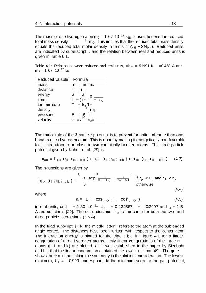
4.2. Interaction potentials 43
The mass of one hydrogen atom, m0 = 1.67 ·10−27 kg, is used to define the reducedtotal mass density ρ∗ = ρσ3/m0. This implies that the reduced total mass densityequals the reduced total molar density in terms of (NH + 2NH2
). Reduced unitsare indicated by superscript ∗, and the relation between real and reduced units isgiven in Table 6.1.
Table 4.1: Relation between reduced and real units, ε/kB = 51991 K, σ=0.458 A andm0 = 1.67 · 10−27 kg.
Reduced vaiable Formulamass m∗ = m/m0
distance r∗ = r/σenergy u∗ = u/ε
time t∗ = (t/σ)√ε/m0
temperature T ∗ = kBT/εdensity ρ∗ = ρσ3/m0
pressure P ∗ = Pσ3/ε
velocity v∗ =v√m0/ε
The major role of the 3-particle potential is to prevent formation of more than onebond to each hydrogen atom. This is done by making it energetically non-favorablefor a third atom to be close to two chemically bonded atoms. The three-particlepotential given by Kohen et al. [29] is:
u(3) = hi,j,k(rij , rjk, θi,j,k) + hj,i,k(rji, rik, θj,i,k) + hi,k,j(rik, rkj , θi,k,j) (4.3)
The h-functions are given by
hj,i,k(rji, rik, θj,i,k) =
{λa exp
[γ3
(rji−rc) + γ3(rik−rc)
]if rji < rc and rik < rc
0 otherwise(4.4)
wherea =
[1 + µ cos(θj,i,k) + ν cos2(θj,i,k)
](4.5)
in real units, and λ = 2.80 · 10−21 kJ, µ = 0.132587, ν = −0.2997 and γ3 = 1.5A are constants [29]. The cut-off distance, rc, is the same for both the two- and
three-particle interactions (2.8 A).
In the triad subscript j, i, k the middle letter i refers to the atom at the subtendedangle vertex. The distances have been written with respect to the center atom.The interaction energy is plotted for the triad j, i, k in Figure 4.1 for a linearconfiguration of three hydrogen atoms. Only linear configurations of the three Hatoms (j, i and k) are plotted, as it was established in the paper by Siegbahnand Liu that the linear configuration contained the lowest minima [49]. The figureshows three minima, taking the symmetry in the plot into consideration. The lowestminimum, U∗1 = −0.999, corresponds to the minimum seen for the pair potential,
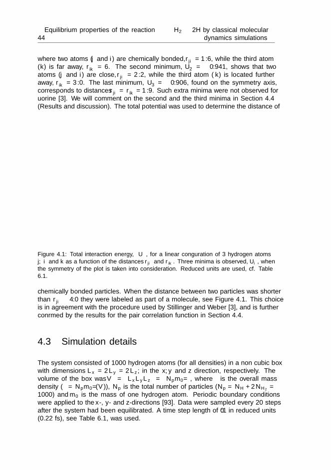
44Equilibrium properties of the reaction H2 2H by classical molecular
dynamics simulations
where two atoms (j and i) are chemically bonded, r∗ji = 1.6, while the third atom(k) is far away, r∗ik = 6. The second minimum, U∗2 = −0.941, shows that twoatoms (j and i) are close, r∗ji = 2.2, while the third atom (k) is located furtheraway, r∗ik = 3.0. The last minimum, U∗3 = −0.906, found on the symmetry axis,corresponds to distances r∗ji = r∗ik = 1.9. Such extra minima were not observed forfluorine [3]. We will comment on the second and the third minima in Section 4.4(Results and discussion). The total potential was used to determine the distance of
Figure 4.1: Total interaction energy, U∗, for a linear configuration of 3 hydrogen atomsj, i and k as a function of the distances r∗ji and r∗ik. Three minima is observed, U∗i , whenthe symmetry of the plot is taken into consideration. Reduced units are used, cf. Table6.1.
chemically bonded particles. When the distance between two particles was shorterthan r∗ji ≤ 4.0 they were labeled as part of a molecule, see Figure 4.1. This choiceis in agreement with the procedure used by Stillinger and Weber [3], and is furtherconfirmed by the results for the pair correlation function in Section 4.4.
4.3 Simulation details
The system consisted of 1000 hydrogen atoms (for all densities) in a non cubic boxwith dimensions Lx = 2Ly = 2Lz, in the x, y and z direction, respectively. Thevolume of the box was V = LxLyLz = Npm0/ρ, where ρ is the overall massdensity (ρ = Npm0/(V )), Np is the total number of particles (Np = NH + 2NH2
=1000) and m0 is the mass of one hydrogen atom. Periodic boundary conditionswere applied to the x-, y- and z-directions [93]. Data were sampled every 20 stepsafter the system had been equilibrated. A time step length of 0.1 in reduced units(0.22 fs), see Table 6.1, was used.

4.3. Simulation details 45
The velocity Verlet algorithm [94] was used to integrate Newton’s equations ofmotion. A list of all pairs who were closer to each other than a set distance,r∗list = 6.5, was made to save computational time, as many particles are furtheraway from each other than the cut-off distance, r∗c = 6.11. Pair interactions werethen only calculated when r∗ ≤ r∗list. A similar algorithm, called NEIGHBOUR3,which was developed by Xu et al. [31], was used to compute 3-particle interactions.In this algorithm a list of triplets is made by combining pairs from the pair list,which have one particle in common. As long as the displacement of the particleswas less than half of r∗list − r∗c = 0.4, we did not need to update the two lists. Thisprocedure avoided unnecessary calculation of particle interactions.
The program gave the temperatures in the box within ±0.1 %. During the equi-libration period the temperature was scaled to the set temperature every step byvelocity scaling. After this, the temperature was adjusted every 100 steps, by scal-ing the velocities with the scaling factor given in Eq. (4.6), to maintain the wantedtemperature [28].
scale =√Tinst/Twanted (4.6)
Here Tinst is the instantaneous temperature and Twanted is the wanted tempera-ture. This does not give a perfect canonical distribution, but we assume that theinfluence of this procedure on the calculated structural- and thermodynamic prop-erties is negligible. In order to test system size dependence, we repeated some ofthe equilibrium simulations for the same density with 4096 particles.
The pair correlation function along with the dissociation constant and reactionenthalpy was studied at a density just below the triple point density (ρ∗ = 0.004)and approximately a fourth of this density (ρ∗ = 0.0011), following the proceduresof Stillinger and Weber [3]. For both densities temperatures were chosen in therange 0.003 ≤ T ∗ ≤ 0.3. Additionally, a run was performed near the triple pointof the molecular fluid (ρ∗ = 0.004 and T ∗ = 0.000268).
For the calculation of the pressure (with the different contributions), densities inthe range 0.00001 ≤ ρ∗ ≤ 0.004 were studied at T ∗ = 0.03. For the densities,ρ∗ = 0.0011 and 0.004 additional runs in temperature range 0.002 ≤ T ∗ ≤ 0.4 wereperformed.
For the high density cases, 0.0003 ≤ ρ∗ ≤ 0.004, three million MD steps were usedfor equilibration of the system and the simulations were run a total of five millionsteps, including the equilibration. For the lower density cases, 0.00001 ≤ ρ∗ ≤0.0001, up to seven million MD steps were used for equilibration, and a total of upto ten million steps were used for the simulation run.
Figure 4.2 shows snapshots from the simulations for the reduced densities ρ∗ = 0.0011(left) and ρ∗ = 0.004 (right) at T ∗ = 0.003 (T = 156 K). We see that the highdensity system is a dense liquid, while the low density system can be compared toa compressed gas.
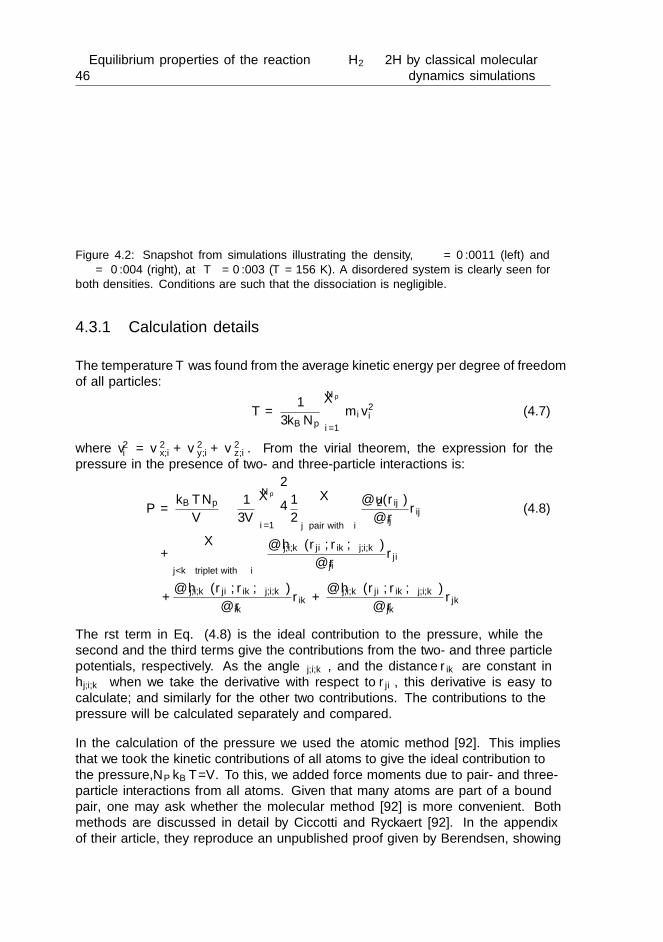
46Equilibrium properties of the reaction H2 2H by classical molecular
dynamics simulations
Figure 4.2: Snapshot from simulations illustrating the density, ρ∗ = 0.0011 (left) andρ∗ = 0.004 (right), at T ∗ = 0.003 (T = 156 K). A disordered system is clearly seen forboth densities. Conditions are such that the dissociation is negligible.
4.3.1 Calculation details
The temperature T was found from the average kinetic energy per degree of freedomof all particles:
T =1
3kBNp
Np∑
i=1
miv2i (4.7)
where v2i = v2
x,i+ v2y,i+ v2
z,i. From the virial theorem, the expression for thepressure in the presence of two- and three-particle interactions is:
P =kBTNpV
− 1
3V
Np∑
i=1
1
2
∑
j pair with i
∂u2(rij)
∂rijrij (4.8)
+∑
j<k triplet with i
(∂hj,i,k(rji, rik, θj,i,k)
∂rjirji
+∂hj,i,k(rji, rik, θj,i,k)
∂rikrik +
∂hj,i,k(rji, rik, θj,i,k)
∂rjkrjk
)]
The first term in Eq. (4.8) is the ideal contribution to the pressure, while thesecond and the third terms give the contributions from the two- and three particlepotentials, respectively. As the angle θj,i,k, and the distance rik are constant inhj,i,k when we take the derivative with respect to rji, this derivative is easy tocalculate; and similarly for the other two contributions. The contributions to thepressure will be calculated separately and compared.
In the calculation of the pressure we used the atomic method [92]. This impliesthat we took the kinetic contributions of all atoms to give the ideal contribution tothe pressure, NP kBT/V . To this, we added force moments due to pair- and three-particle interactions from all atoms. Given that many atoms are part of a boundpair, one may ask whether the molecular method [92] is more convenient. Bothmethods are discussed in detail by Ciccotti and Ryckaert [92]. In the appendixof their article, they reproduce an unpublished proof given by Berendsen, showing
4.4. Results and Discussion 47
that both definitions give the same pressure. As we calculate the forces, positionsand velocities of all atoms in the MD simulation, it is natural to use the atomicmethod here.
The molar density, ck, of component k is:
ck =NkNAV
(4.9)
where Nk is the number of particles of component k (H or H2). Furthermore NAis Avogadro’s number. The mass density of the system can be found from
ρ =Npm0
V(4.10)
The thermodynamic equilibrium constant, Kth, can be found from the dissociationconstant, Kx, and the activity coefficients according to
Kth =x2
H
xH2
γ2H
γH2
≡ Kxγ2
H
γH2
(4.11)
The equilibrium constant can then be used to find Gibbs energy of the reaction
∆rG = ∆rG◦ +RT lnKth (4.12)
The standard reaction enthalpy can then be found from the van’t Hoff equation atconstant pressure [
d lnKth
d(1/T )
]
P
= −∆rH◦
R(4.13)
At chemical equilibrium, ∆rG = 0 and hence ∆rG◦ = −RT lnKth. For an ideal
mixture γ2H/γH is unity and Kx = Kth. When the ratio of the activity coefficients
at constant pressure is constant, we can find ∆rH◦ from the van’t Hoff equation
using Kx. We shall seek to find such conditions.
4.4 Results and Discussion
4.4.1 Pair correlation functions
The atom-atom pair correlation function, g(r), for the hydrogen atoms, includingatoms that are part of a molecule, describes the correlation of two atoms as afunction of the distance. A deviation in the pair correlation function from unityindicates correlations between particles due to intermolecular interactions. Hence,the pair correlation function gives information about the number of chemicallybonded atoms and the distance between bonded atoms, and their neighboring atoms[3,31].

48Equilibrium properties of the reaction H2 2H by classical molecular
dynamics simulations
0
1
2
3
4
5
0 2 4 6 8 10 12 14 16 18 20
g(r)
r*ij
Figure 4.3: Pair correlation function near the triple point of the molecular fluid. T ∗=0.000268 (T = 14 K), ρ∗=0.004 (ρH = 0.0695 g cm−3).
The pair correlation function near the triple point of the molecular fluid, ρ∗ = 0.004and T ∗ = 0.000268, is given in Figure 4.3. The figure shows a very high peak aroundr∗ij = 1.6 and several minor peaks before a plateau is reached.
The high peak represents chemically bonded pairs and its area reflects the fact thatthere are 500 molecules in the system (no dissociation at this low temperature). Thefirst three peaks in Figure 4.3 can be directly related to Figure 4.1, the potentialenergy of linear arrays of 3 hydrogen atoms. We see here that the distance r∗ij = 1.6corresponds to the arrangement with the lowest energy, U∗1 = −0.999. Two atomsare bound at this distance while the third atom is found at a distance r∗ik = 6.This is compatible with the first high peak. This part is similar to the resultsof Stillinger and Weber for fluorine [3]. They observed no additional peaks intheir pair correlation functions for fluorine however; in agreement with one singleminimum in their total potential.
The second minimum U∗2 = −0.941 in Figure 4.1 leads to two small peaks in thepair correlation function in Figure 4.3 at reduced distances r∗ij = 2.2 and 3.0.The third minimum U∗3 = −0.906 in Figure 4.1 has no clear impact on the paircorrelation function in Figure 4.3. The small peak around r∗ij ≈ 5 cannot be tracedto a minimum in the energy landscape. For a temperature of 14 K, the de Brogliewavelength for H is 10.15 in reduced units (Λ = h/
√2πm0kBT , where h is Planck’s
constant, and m0 the mass of one hydrogen atom). For this temperature theclassical calculation is therefore not adequate. The triplet structure is an artefactof this. In the simulations these linear formations of triplets, when they appear,

4.4. Results and Discussion 49
are stable over the whole simulations, as the kinetic energy of the particles is to lowto move to another minimum. We therefore interpret the peaks beyond r∗ij = 4 asdue to intermolecular short-range order of chemically bonded pairs. The reason todo the classical calculation for this low temperature is to compare the results withthe results for fluorine in the paper by Stillinger and Weber [3]. The similarity ofthe results validates our analysis.
It is interesting to observe that the system develops an effective excluded volumediameter. The pair potential is zero at a distance 1 in reduced units. When three-particle interactions are included, the molecule obtains an effective excluded volumediameter of about 6, as seen from Figure 4.3, where the pair correlation functionis approximately zero in the region 2.2 < r∗ij < 6, but rises sharply at 6. This
value in real units is 2.748 A, a value in good agreement with the value 2.7 A givenby Labet et al. [84] for the second shortest H-H separation at 1 GPa. Moreover,
it compares well with the value 2.81 A given by Allen and Tildesley [28] for aLennard-Jones potential of molecular hydrogen. This means that our model forthe chemical reaction at a meso-level is consistent with a coarser level fluid modelof the molecular system, making this part of the model realistic.
Figure 4.4 shows the pair correlation function at T ∗ = 0.003, for both ρ∗ = 0.004(Figure 4.4(a)) and ρ∗ = 0.0011 (Figure 4.4(b)). When we compare the two paircorrelation functions for the two densities in Figure 4.4 we see that they have thesame general trend. A large and narrow peak can be seen at r∗ij = 1.6 in bothcases. This peak is broadest at the lower density (ρ∗ = 0.0011, Figure 4.4(b)). Atthe higher density (ρ∗ = 0.004) it is just slightly broader than in Figure 4.3. Abroadening is also observed in the rest of the structure, when we compare Figures4.4(a) and 4.4(b) to the counterpart in Figure 4.3. In the high density results,ρ∗ = 0.004 in Figure 4.4(a), the peak at r∗ij = 3 has been incorporated into the smallpeak at r∗ij = 2.2 as a shoulder. For the low density, ρ∗ = 0.0011 in Figure 4.4(b),no distinct extra peak is observed, but a broad shoulder remains. A broadeningof peaks take place, due to increase in the temperature as well as to the reductionin density. For a temperature of 156 K, the de Broglie wavelength for H is 3.03 inreduced units. For this temperature the classical calculation is therefore also notadequate. We refer to the discussion for 14 K above. The pair correlation functiongoes smoothly to unity as expected at about r∗ij = 10 for the high density, andat about 8 for the low density. For neither density, dissociation was observed, cf.Tables 6.4 and 6.3.
The pair correlation function at T ∗ = 0.03 is given in Figure 4.5, for the highdensity, ρ∗ = 0.004 in Figure 4.5(a), and the low density, ρ∗ = 0.0011 in Figure4.5(b). No dissociation was observed for either density, see Tables 6.4 and 6.3. Themain peak at r∗ij = 1.6, corresponding to the chemically bonded atoms, has furtherbroadened for both densities compared to Figures 4.4(a) and 4.4(b). The two peaksdue to the second potential minimum have disappeared. This is clearly due to theincrease in the temperature. The area under the pair correlation function from2.4 ≤ r∗ij ≤ 5 is zero for both densities. From r∗ij around 9 the correlation functionis roughly equal to one for both densities.
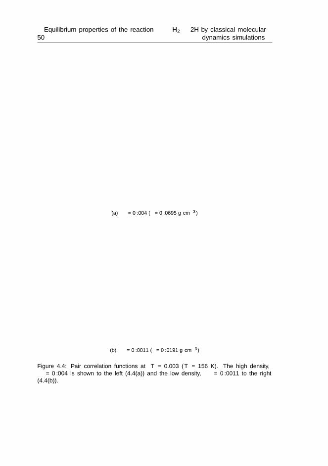
50Equilibrium properties of the reaction H2 2H by classical molecular
dynamics simulations
0
1
2
3
4
5
0 2 4 6 8 10 12 14 16 18 20
g(r)
r*ij
(a) ρ∗ = 0.004 (ρ = 0.0695 g cm−3)
0
1
2
3
4
5
0 2 4 6 8 10 12 14 16 18 20
g(r)
r*ij
(b) ρ∗ = 0.0011 (ρ = 0.0191 g cm−3)
Figure 4.4: Pair correlation functions at T ∗= 0.003 (T = 156 K). The high density,ρ∗ = 0.004 is shown to the left (4.4(a)) and the low density, ρ∗ = 0.0011 to the right(4.4(b)).
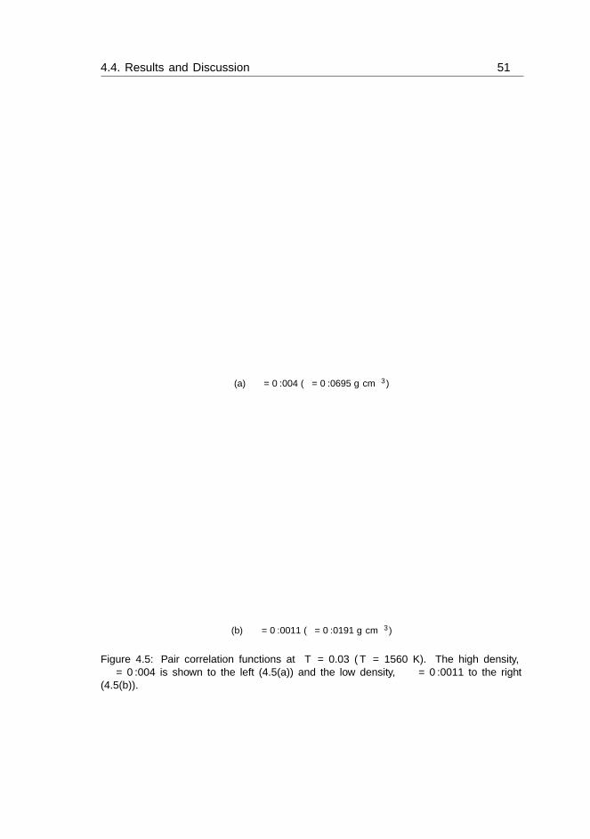
4.4. Results and Discussion 51
0
1
2
3
4
5
0 2 4 6 8 10 12 14 16 18 20
g(r)
r*ij
(a) ρ∗ = 0.004 (ρ = 0.0695 g cm−3)
0
1
2
3
4
5
0 2 4 6 8 10 12 14 16 18 20
g(r)
r*ij
(b) ρ∗ = 0.0011 (ρ = 0.0191 g cm−3)
Figure 4.5: Pair correlation functions at T ∗= 0.03 (T = 1560 K). The high density,ρ∗ = 0.004 is shown to the left (4.5(a)) and the low density, ρ∗ = 0.0011 to the right(4.5(b)).
52Equilibrium properties of the reaction H2 2H by classical molecular
dynamics simulations
Figure 4.6 shows the pair correlation functions for both the high density, ρ∗ = 0.004(Figure 4.6(a)), and the low density, ρ∗ = 0.0011 (Figure 4.6(b)), at T ∗ = 0.3.The correlation function is near unity for r∗ij > 6, as one should expect for thistemperature. But the pair correlation is no longer zero when 2.2 < r∗ij < 5. This isa sign of the reaction taking place. If we compare the high- and low density figures,we see that the main difference is the intensity and broadness of the first peak, asthe main peak in Figure 4.6(b) is both broader and has a lower intensity than it’shigh density counterpart. Compatible with this we find that more particles arebound at the low density. For the high density in Figure 4.6(a), we observe 23 %dissociation (232.4 atoms), while for the low density, in Figure 4.6(b), a dissociationof 47 % (468.7 atoms) is observed, cf. Tables 6.4 and 6.3.
In the counting procedure used, we label all particles as either atoms or molecules.If, during the simulation, the distance between two atoms is less than 4, they arelabelled as molecules. At the end of every 20 time steps, we count the number ofatoms. The rest is then counted as molecules. At higher temperatures, bonds arecontinuously formed and broken, and as Stillinger and Weber [2] say, this countingprocedure will give a reasonable, but still approximate value of the number ofmolecules. We estimate the accuracy to be within ± 1 %.
In summary, from Figures 4.3 – 4.6, we conclude that the three-particle potentialhas a large ordering effect on the molecules, in agreement with earlier observations[3]. The effective excluded volume diameter of the molecule becomes 6 in reducedunits as a result of the three particle interaction, a value in agreement with theinterparticle distance of the Lennard-Jones potential for molecular hydrogen [28].The ordering effect was observed to decrease with increasing temperature.
At very low temperature (14 K and 156 K) quantum effects becomes importantand for this reason our classical description leads to triplets which is an artefact ofthis. At very high temperatures, above 20 000 K, we see from the phase diagramsthat we might be entering the plasma region of hydrogen [95–97]. At the highesttemperature and density considered here (15 600 K and ρ = 0.0695 g cm−3), weare however well within the region of the atomic fluid, and thus we expect that ourmodel is able to predict the properties of hydrogen.
For all conditions, bound particles were be determined for a set distance r∗ij ≤ 4. Fortemperatures showing the behaviour illustrated by Figure 4.6 we are dealing with achemical reaction, and can find the fraction of molecules by counting the particleswhich obey this inequality. The role of the two- and three particle interactions willbe examined further below.
4.4.2 The Contributions to the Pressure in a Reacting Mix-ture
The overall pressure, Ptot, in the calculation is a sum of the kinetic (or ideal)pressure, Pideal, and the contributions from the two- and three particle potentials,

4.4. Results and Discussion 53
0
1
2
3
4
5
0 2 4 6 8 10 12 14 16 18 20
g(r)
r*ij
(a) ρ∗ = 0.004 (ρ = 0.0695 g cm−3)
0
1
2
3
4
5
0 2 4 6 8 10 12 14 16 18 20
g(r)
r*ij
(b) ρ∗ = 0.0011 (ρ = 0.0191 g cm−3)
Figure 4.6: Pair correlation functions at T ∗= 0.3 (T = 15600 K). The high density,ρ∗ = 0.004 is shown to the left (4.6(a)) and the low density, ρ∗ = 0.0011 to the right(4.6(b)).

54Equilibrium properties of the reaction H2 2H by classical molecular
dynamics simulations
P2part and P3part, see Eq. (4.8). The relative magnitude of these contributionsto the overall pressure at T ∗ = 0.03 was calculated and is given in Figure 4.7 fordensities in the range 0.00001 ≤ ρ∗ ≤ 0.004. The different contributions, Pi, to thepressure have been divided by the ideal pressure (Pi/Pideal) to be able to comparethe contributions at different densities relative to each other. As a consequence theideal contribution, Pideal (from the first part of Eq. (4.8)) in Figure 4.7 is equal to1 for all densities. Important in Berendsen’s proof of the equality of the atomic and
-0.5
0
0.5
1
1.5
2
1e-05 0.0001 0.001 0.01
Pi /P
idea
l
ρ*
PtotPidealP2partP3part
Figure 4.7: The total pressure, Ptot, and the contribution from the ideal part, Pideal, andtwo- and three particle interactions, P2part and P3part at T ∗ = 0.03 as a function of thedensity of the system, 0.00001 ≤ ρ∗ ≤ 0.004. The densities are plotted using log scale.All pressures have been normalized with respect to the ideal pressure, giving Pideal = 1for all densities.
molecular method for pressure calculations (see Ciccotti and Ryckaert [92]), is thatthe intramolecular two particle forces give a negative contribution to the pressure.In good approximation, it replaces the kinetic pressure of two atoms 2kBT/V bythe kinetic pressure of one molecule kBT/V . It follows that the contribution tothe pressure due to pair interaction is negative, and in essence reduces the kineticpressure from (NH + 2NH2
)kBT/V to (NH +NH2)kBT/V . The contribution from
the pair potential to the pressure in Figure 4.7 is negative and approximately halfthe size of the ideal contribution, cf. [92]. So it is playing an important role tolower the overall pressure.
The role of the three-particle interaction is very different. As we have seen fromthe pair correlation functions (see Section 4.4.1), no particles aside from the bound
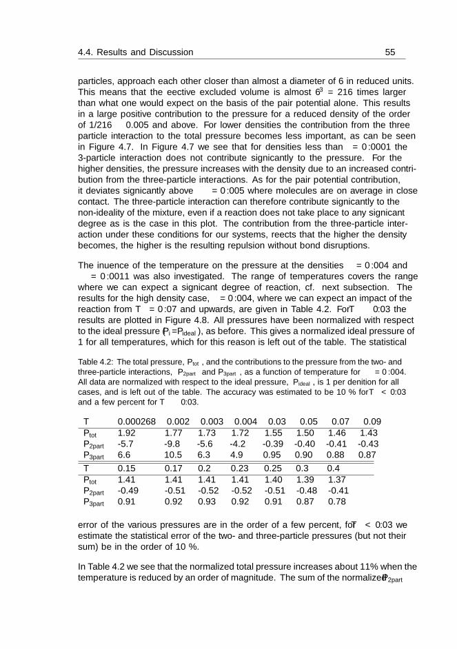
4.4. Results and Discussion 55
particles, approach each other closer than almost a diameter of 6 in reduced units.This means that the effective excluded volume is almost 63 = 216 times largerthan what one would expect on the basis of the pair potential alone. This resultsin a large positive contribution to the pressure for a reduced density of the orderof 1/216 ≈ 0.005 and above. For lower densities the contribution from the threeparticle interaction to the total pressure becomes less important, as can be seenin Figure 4.7. In Figure 4.7 we see that for densities less than ρ∗ = 0.0001 the3-particle interaction does not contribute significantly to the pressure. For thehigher densities, the pressure increases with the density due to an increased contri-bution from the three-particle interactions. As for the pair potential contribution,it deviates significantly above ρ∗ = 0.005 where molecules are on average in closecontact. The three-particle interaction can therefore contribute significantly to thenon-ideality of the mixture, even if a reaction does not take place to any significantdegree as is the case in this plot. The contribution from the three-particle inter-action under these conditions for our systems, reflects that the higher the densitybecomes, the higher is the resulting repulsion without bond disruptions.
The influence of the temperature on the pressure at the densities ρ∗ = 0.004 andρ∗ = 0.0011 was also investigated. The range of temperatures covers the rangewhere we can expect a significant degree of reaction, cf. next subsection. Theresults for the high density case, ρ∗ = 0.004, where we can expect an impact of thereaction from T ∗ = 0.07 and upwards, are given in Table 4.2. For T ∗ ≥ 0.03 theresults are plotted in Figure 4.8. All pressures have been normalized with respectto the ideal pressure (Pi/Pideal), as before. This gives a normalized ideal pressure of1 for all temperatures, which for this reason is left out of the table. The statistical
Table 4.2: The total pressure, Ptot, and the contributions to the pressure from the two- andthree-particle interactions, P2part and P3part, as a function of temperature for ρ∗ = 0.004.All data are normalized with respect to the ideal pressure, Pideal, is 1 per definition for allcases, and is left out of the table. The accuracy was estimated to be 10 % for T ∗ < 0.03and a few percent for T ∗ ≥ 0.03.
T ∗ 0.000268 0.002 0.003 0.004 0.03 0.05 0.07 0.09Ptot 1.92 1.77 1.73 1.72 1.55 1.50 1.46 1.43P2part -5.7 -9.8 -5.6 -4.2 -0.39 -0.40 -0.41 -0.43P3part 6.6 10.5 6.3 4.9 0.95 0.90 0.88 0.87
T ∗ 0.15 0.17 0.2 0.23 0.25 0.3 0.4Ptot 1.41 1.41 1.41 1.41 1.40 1.39 1.37P2part -0.49 -0.51 -0.52 -0.52 -0.51 -0.48 -0.41P3part 0.91 0.92 0.93 0.92 0.91 0.87 0.78
error of the various pressures are in the order of a few percent, for T ∗ < 0.03 weestimate the statistical error of the two- and three-particle pressures (but not theirsum) be in the order of 10 %.
In Table 4.2 we see that the normalized total pressure increases about 11% when thetemperature is reduced by an order of magnitude. The sum of the normalized P2part

56Equilibrium properties of the reaction H2 2H by classical molecular
dynamics simulations
and P3part, which equals the normalized total pressure minus 1, similarly increaseswhen the temperature decreases. For T ∗ between 0.03 and 0.4 the change of thevalues of the normalized P2part and P3part is similarly rather small. The absolutevalue of these contributions is between zero and one for these temperatures. Forlower temperatures the normalized P2part and P3part both increase by up to an orderof magnitude without a similar increase in their sum. For these low temperatures,all hydrogen atoms are bound in molecules.
At low temperatures a particular property of this system affects the results. Atthese temperatures, there are no atoms in the system, and no reaction is going on.Most of the atoms, once they are bound to each other in a molecule, remain boundduring the whole simulation. Concurrent with this is that also 3 atoms can arrivein the second or third minimum, see Figure 4.1. The occurrence of such tripletswas observed in Figures 4.3 and 4.4 as small side peaks (shoulders) at reduceddistances 2.2 and 3. The number of triplets is small, but they can remain stuck toeach other during the whole simulation at low temperatures. The existence of somepermanent triplets can explain the enormous decrease of the 2 particle contributionand roughly the same increase of the 3 particle contributions, while their sum isonly slightly increased above the higher temperature value. The existence of tripletsis a consequence of the potential we have used. The potential was an analyticalrepresentation of an energy surface generated from quantum mechanics [3], but itmay not represent reality under these extreme conditions. In Figure 4.8, we onlyplot the normalized pressures for the high temperature domain, T ∗ between 0.03and 0.4. The statistical error was estimated to be in the order of a few percentfor T ∗ ≥ 0.03. For lower temperatures the statistical error of the two- and three-particle pressures (but not their sum) was estimated to be in the order of 10 %.
For the low density case, ρ∗ = 0.0011, the total pressure and the different contri-butions to the pressure as a function of temperature is given in Table 4.3 below,and plotted in Figure 4.9 for T ∗ ≥ 0.03. Also here we can expect an impact ofthe reaction from T ∗ = 0.07 and up. From Table 4.3 we see that the normalized
Table 4.3: The total pressure, Ptot and the contributions to the pressure from the two- andthree-particle interactions, P2part and P3part, as a function of temperature for ρ∗ = 0.0011.All data are normalized with respect to the ideal pressure, Pideal. The normalized idealpressure, Pideal, is 1 per definition for all cases, and is left out of the table. The accuracywas estimated to be 10 % for T ∗ < 0.03 and a few percent for T ∗ ≥ 0.03.
T ∗ 0.002 0.003 0.004 0.03 0.05 0.07 0.09Ptot 0.69 0.69 0.68 0.67 0.66 0.66 0.67P2part -2.6 -1.9 -2.9 -0.48 -0.48 -0.48 -0.48P3part 2.3 1.6 2.6 0.15 0.15 0.15 0.15
T ∗ 0.11 0.13 0.15 0.17 0.2 0.25 0.3 0.4Ptot 0.68 0.70 0.73 0.76 0.80 0.85 0.88 0.92P2part -0.47 -0.44 -0.44 -0.42 -0.38 -0.32 -0.27 -0.20P3part 0.16 0.17 0.17 0.18 0.18 0.17 0.15 0.12

4.4. Results and Discussion 57
-1
-0.5
0
0.5
1
1.5
2
0 0.05 0.1 0.15 0.2 0.25 0.3 0.35 0.4
Pi /P
idea
l
T*
PtotPidealP2partP3part
Figure 4.8: The total pressure, Ptot, and the different contributions to the pressure,Pideal and from the two- and three-particle interactions, P2part and P3part as a function oftemperatures for the high density case, ρ∗ = 0.004. All data have been normalized withrespect to the ideal pressure, giving Pideal = 1.
58Equilibrium properties of the reaction H2 2H by classical molecular
dynamics simulations
total pressure is essentially constant at low temperatures (between T ∗ = 0.002 andT ∗ = 0.13) and increases by about 20% when the reduced temperature increases toT ∗ = 0.4. This behavior is different from the result for the higher density, wherethe normalized total pressure decreased when the temperature increased. The sumof the normalized P2part and P3part, which equals the normalized total pressureminus 1, behaves similarly. The value of the normalized P2part is reduced about60% from T ∗ = 0.03 to T ∗ = 0.4, while the value of the normalized P3part remainsessentially constant in this temperature domain. For lower temperatures the nor-malized P2part and P3part both increase by up to an order of magnitude withouta similar increase in their sum. The reason for this is the same as the one givenfor the higher density. In Figure 4.9, we only plot the normalized pressures for thehigh temperature domain, T ∗ between 0.03 and 0.4.
-0.6
-0.4
-0.2
0
0.2
0.4
0.6
0.8
1
1.2
0 0.05 0.1 0.15 0.2 0.25 0.3 0.35 0.4
Pi /P
idea
l
T*
PtotPidealP2partP3part
Figure 4.9: The total pressure, Ptot, and the different contributions to the pressure,Pideal and from the two- and three-particle interactions, P2part and P3part as a function oftemperatures for the low density case, ρ∗ = 0.0011. All data have been normalized withrespect to the ideal pressure, giving Pideal = 1.
For the high density, we see that the relative contributions to the normalized pres-sure are constant, up or down 10%, for T ∗ = 0.03 − 0.4, indicating that γ2
H/γH2
is approximately constant in this range. This indicates that we can use the van’tHoff equation, Eq.(4.13), with Kx, to determine the standard enthalpy of the re-action, and we shall do so below. For the low density, we see the same trend inthe normalized overall pressure for a lower temperature range, 0.03 ≤ T ∗ ≤ 0.13,indicating that γ2
H/γH2 is constant also there.
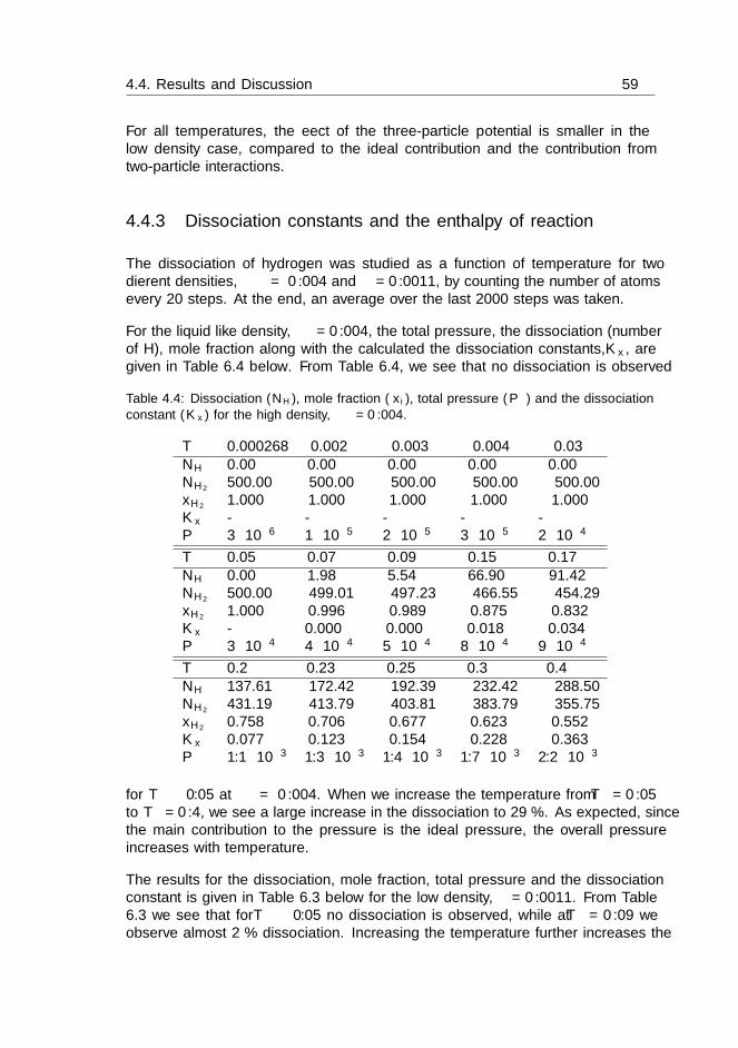
4.4. Results and Discussion 59
For all temperatures, the effect of the three-particle potential is smaller in thelow density case, compared to the ideal contribution and the contribution fromtwo-particle interactions.
4.4.3 Dissociation constants and the enthalpy of reaction
The dissociation of hydrogen was studied as a function of temperature for twodifferent densities, ρ∗ = 0.004 and ρ∗ = 0.0011, by counting the number of atomsevery 20 steps. At the end, an average over the last 2000 steps was taken.
For the liquid like density, ρ∗ = 0.004, the total pressure, the dissociation (numberof H), mole fraction along with the calculated the dissociation constants, Kx, aregiven in Table 6.4 below. From Table 6.4, we see that no dissociation is observed
Table 4.4: Dissociation (NH), mole fraction (xi), total pressure (P ∗) and the dissociationconstant (Kx) for the high density, ρ∗ = 0.004.
T ∗ 0.000268 0.002 0.003 0.004 0.03NH 0.00 0.00 0.00 0.00 0.00NH2
500.00 500.00 500.00 500.00 500.00xH2 1.000 1.000 1.000 1.000 1.000Kx - - - - -P ∗ 3 · 10−6 1 · 10−5 2 · 10−5 3 · 10−5 2 · 10−4
T ∗ 0.05 0.07 0.09 0.15 0.17NH 0.00 1.98 5.54 66.90 91.42NH2
500.00 499.01 497.23 466.55 454.29xH2 1.000 0.996 0.989 0.875 0.832Kx - 0.000 0.000 0.018 0.034P ∗ 3 · 10−4 4 · 10−4 5 · 10−4 8 · 10−4 9 · 10−4
T ∗ 0.2 0.23 0.25 0.3 0.4NH 137.61 172.42 192.39 232.42 288.50NH2
431.19 413.79 403.81 383.79 355.75xH2 0.758 0.706 0.677 0.623 0.552Kx 0.077 0.123 0.154 0.228 0.363P ∗ 1.1 · 10−3 1.3 · 10−3 1.4 · 10−3 1.7 · 10−3 2.2 · 10−3
for T ∗ ≤ 0.05 at ρ∗ = 0.004. When we increase the temperature from T ∗ = 0.05to T ∗ = 0.4, we see a large increase in the dissociation to 29 %. As expected, sincethe main contribution to the pressure is the ideal pressure, the overall pressureincreases with temperature.
The results for the dissociation, mole fraction, total pressure and the dissociationconstant is given in Table 6.3 below for the low density, ρ∗ = 0.0011. From Table6.3 we see that for T ∗ ≤ 0.05 no dissociation is observed, while at T ∗ = 0.09 weobserve almost 2 % dissociation. Increasing the temperature further increases the
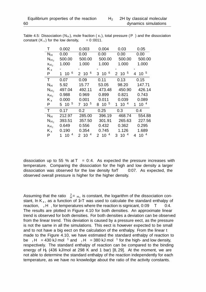
60Equilibrium properties of the reaction H2 2H by classical molecular
dynamics simulations
Table 4.5: Dissociation (NH), mole fraction (xi), total pressure (P ∗) and the dissociationconstant (Kx) for the low density, ρ∗ = 0.0011.
T ∗ 0.002 0.003 0.004 0.03 0.05NH 0.00 0.00 0.00 0.00 0.00NH2
500.00 500.00 500.00 500.00 500.00xH2
1.000 1.000 1.000 1.000 1.000Kx - - - - -P ∗ 1 · 10−6 2 · 10−6 3 · 10−6 2 · 10−5 4 · 10−5
T ∗ 0.07 0.09 0.11 0.13 0.15NH 5.92 15.77 53.05 98.20 147.71NH2 497.04 492.11 473.48 450.90 426.14xH2 0.988 0.969 0.899 0.821 0.743Kx 0.000 0.001 0.011 0.039 0.089P ∗ 5 · 10−5 7 · 10−5 8 · 10−5 1 · 10−4 1 · 10−4
T ∗ 0.17 0.2 0.25 0.3 0.4NH 212.97 285.00 396.19 468.74 554.88NH2 393.51 357.50 301.91 265.63 227.56xH2 0.649 0.556 0.432 0.362 0.295Kx 0.190 0.354 0.745 1.126 1.689P ∗ 1 · 10−4 2 · 10−4 2 · 10−4 3 · 10−4 4 · 10−4
dissociation up to 55 % at T ∗ = 0.4. As expected the pressure increases withtemperature. Comparing the dissociation for the high and low density a largerdissociation was observed for the low density for T ∗ ≥ 0.07. As expected, theobserved overall pressure is higher for the higher density.
Assuming that the ratio γ2H/γH2 is constant, the logarithm of the dissociation con-
stant, lnKx, as a function of 1/T was used to calculate the standard enthalpy ofreaction, ∆rH
◦, for temperatures where the reaction is significant, 0.09 ≤ T ∗ ≤ 0.4.The results are plotted in Figure 4.10 for both densities. An approximate lineartrend is observed for both densities. For both densities a deviation can be observedfrom the linear trend. This deviation is caused by a pressure effect, as the pressureis not the same in all the simulations. This effect is however expected to be smalland to not have a big effect on the calculation of the enthalpy. From the linear fitmade to the Figure 4.10, we have estimated the standard enthalpy of reaction tobe ∆rH
◦ = 430 kJ mol−1 and ∆rH◦ = 380 kJ mol−1 for the high- and low density,
respectively. The standard enthalpy of reaction can be compared to the bindingenergy of H2 (436 kJ/mol at 298 K and 1 bar) [8, 29]. At the moment, we arenot able to determine the standard enthalpy of the reaction independently for eachtemperature, as we have no knowledge about the ratio of the activity constants.

4.5. Conclusion 61
-10
-8
-6
-4
-2
0
2
5e-05 0.0001 0.00015 0.0002
ln(K
x)
1/T [K-1]
ρ*=0.0011
ρ*=0.004
Figure 4.10: The natural logarithm of the dissociation constant, lnKx, plotted as a func-tion of the inverse temperature (T ∗ = 0.09− 0.3)
4.5 Conclusion
We have seen in the preceding sections that a classical MD model is able to capturethe essential properties of a chemical reaction at equilibrium; namely its dissocia-tion, enthalpy of reaction, and pressure and temperature variations. This was madepossible by adding to the pair potential a three-particle interaction potential. Thesystem behaviour on the meso-scale, characterized here by pair correlation func-tions, was found to be compatible with a coarser scale description, where the pairpotential is the sole potential needed. In particular, the effective excluded volumediameter of the molecule was in agreement with the Lennard-Jones diameter usedby others [28,84] to model fluid hydrogen. For low temperatures (14 K and 156 K)the de Broglie wavelength was large compared to the binding distance. For thesetemperatures the classical calculation is not appropriate. The triplet state foundin the calculation at these temperatures is an artefact of this.
For two densities, ρ∗ = 0.0011 and ρ∗ = 0.004, and a series of temperatures, thethree-particle interaction was found to have a large positive impact on the overallpressure. Assuming that the activity coefficient ratio was constant, the standardenthalpy of the reaction was estimated from van’t Hoff equation to be 430 kJ/mol(ρ∗ = 0.004) and 380 kJ/mol (ρ∗ = 0.0011).
We have thus seen that a reacting mixture can be well modelled in a classical way,if the temperature is not to low. This opens up the possibility for dealing withproblems related to reaction, diffusion, heat conduction, even thermal diffusion, and
62Equilibrium properties of the reaction H2 2H by classical molecular
dynamics simulations
interface transport, in problems which are central to chemical reactor (combustion)technology. This is in complete accordance with the view of Stillinger and coworkers[3,29]. To the best of our knowledge the idea of these authors have not been taken tothe next steps yet. Neither has the impact of a three-particle interaction potentialbeen discussed in the literature, see however [31]. A simple model for the chemicalreaction as presented here for hydrogen, will allow its introduction in fluid modellingat large. The model may facilitate simultaneous studies of reaction and diffusionunder various non-equilibrium conditions, and serve as a benchmark for quantummechanical calculations of reactions.
Acknowledgement
P. O. Astrand is thanked for clarifying discussions concerning the potential andthe resulting triplet structures. The authors are grateful to the Storforsk ProjectTransport no 167336 from NFR and the Department of Chemistry, NTNU, forfinancial support.
Chapter 5
Partial Molar Enthalpies andReaction Enthalpies FromEquilibrium MolecularDynamics Simulation
Sondre K. Schnell1,2,3, Ragnhild Skorpa3, Dick Bedeaux1,Signe Kjelstrup1,3 Thijs J. H. Vlugt1 and Jean-Marc
Simon4,
1. Process & Energy Laboratory, Delft University of Technology,Leeghwaterstraat 39, 2628CB Delft, The Netherlands
2. Department of Chemical and Biomolecular Engineering,University of California, Berkeley, Berkeley,
California 94720, United States
3. Department of Chemistry,Norwegian University of Science and Technology,
NO-7491 Trondheim, Norway
4. Laboratorie Interdisciplinaire Carnot de Bourgogne,UMR, CNRS-Universite de Bourgogne, Dijon, France.
This chapter was published in J. Chem. Phys (2014) 141:144501
64Partial Molar Enthalpies and Reaction Enthalpies From Equilibrium
Molecular Dynamics Simulation
Abstract
We present a new molecular simulation technique for determining partial molarenthalpies in mixtures of gases and liquids from single simulations, without relyingon particle insertions, deletions, or identity changes. The method can also beapplied to systems with chemical reactions. We demonstrate our method for binarymixtures of WCA particles by comparing with conventional simulation techniques,as well as for a simple model that mimics a chemical reaction. The method considerssmall subsystems inside a large reservoir (i.e. the simulation box), and uses theconstruction of Hill to compute properties in the thermodynamic limit from small-scale fluctuations. Results obtained with the new method are in excellent agreementwith those from previous methods. Especially for modeling chemical reactions, ourmethod can be a valuable tool for determining reaction enthalpies directly from asingle MD simulation.
5.1 Introduction
The state-function enthalpy, H, is an important thermodynamic property in awide variety of applications, ranging from chemical engineering to biology [98–100].From knowledge of the enthalpy as a function of composition, one can determinethe partial molar enthalpy of a component in a mixture. This quantity is central tounderstand thermodynamics of mixtures and chemical reactions under equilibriumand non-equilibrium conditions [12, 100]. In most applications, the temperatureT and pressure p are constant, meaning that it is convenient to express the totaldifferential of the enthalpy H(T, p,Ni) like:
dH =
(∂H
∂T
)
p,Ni
dT +
(∂H
∂p
)
T,Ni
d p+
n∑
i=1
(∂H
∂Ni
)
T,p,Nj 6=i
dNi, (5.1)
where Ni is the number of particles of component i and n the number of differ-ent species. Only component contributions remain at constant temperature andpressure, leading to the integrated version
H =n∑
i=1
NiHi, (5.2)
with Hi =(∂H∂Ni
)T,p,Nj 6=i
being the partial enthalpy per particle of component i
at constant T , p, Nj 6=i, the partial molar enthalpy is obtained by multiplying Hi
with the Avogadro number. In the following, in particular in the Chapter 5.4, wewill transform partial enthalpies at constant T , V , µj 6=i to constant T , V , Nj 6=ifinally to constant T , p, Nj 6=i, µj being the chemical potential of component j. Weshall use the name ”partial enthalpy” for all these properties and reserve the name”partial molar enthalpy” of component i for derivatives of H that refer to T, p and
5.1. Introduction 65
Nj 6=i constant, whatever it is per particle or per mole of particle.Partial molar enthalpies are normally obtained using numerical derivation of thetotal enthalpy H with respect to one component [14]. For species that take partin a chemical reaction at equilibrium, such a procedure is not straightforward, asit is difficult, if not impossible, to keep the number of particles of one componentconstant, while varying the other.
Molecular simulations are helpful in building of reliable databases of thermody-namic data. Several methods have been developed for calculating Hi in sys-tems without chemical reactions. These methods rely on differentiating the to-tal enthalpy H with respect to composition, or particle insertions or identitychanges [19,21]. To the best of our knowledge, there are no techniques available todirectly obtain partial molar enthalpies of reacting species, or reaction enthalpies.
Most classical molecular dynamics (MD) simulations do not allow for the formationand breaking of chemical bonds. Nevertheless, a few force fields mimic chemicalreactions using classical interaction potentials, like ReaxFF [38], REBO [39], andAIREBO [40]. A classical three-body interaction potential [3, 29, 32, 48] was alsoused to model chemical reactions 2F F2 [3, 31] and 2H H2 [48]. As thereaction enthalpy is needed to calculate how the equilibrium constant changes withtemperature, it would be very useful to compute it from a single simulation.
The aim of this paper is to present a new molecular simulation technique for deter-mining partial molar enthalpies. The method presented in this paper can also beapplied to systems with chemical reactions. We will demonstrate our method forbinary mixtures of WCA particles [101], as well as for a simple model that mimicsa chemical reaction. The method considers small subsystems in a large reservoir(i.e. the simulation box), and uses the construction of Hill [50] to compute thermo-dynamic properties in the thermodynamic limit from small-scale fluctuations. Themethod largely expands the work on small systems by Schnell et al. [22–24,56,102].
The subsystem refers to an open volume (or area element) with a linear size ofthe order of 1 to 10 molecular diameters, inside a much larger simulation box (areservoir). We will derive how energy and particle fluctuations inside the subsystemcan be used to obtain thermodynamic properties in the grand-canonical ensemble.This ensemble differs from the ensemble specified above (constant T, p,Nj) in whichpartial molar enthalpies are defined. The total differential of the enthalpy in thegrand-canonical ensemble equals
dH =
(∂H
∂T
)
V,µi
dT +
(∂H
∂V
)
T,µi
dV +
n∑
i=1
(∂H
∂µi
)
T,V,µj 6=i
dµi. (5.3)
The partial derivatives with respect to chemical potentials of component i, µi, areobtained for conditions T and V constant. To find the partial molar enthalpiesdefined in Eq. (5.1), we need to relate them to the partial derivatives in Eq. (5.3).We will show how Legendre transformations can be used to convert the partialderivatives in Eq. (5.3) to partial molar enthalpies.

66Partial Molar Enthalpies and Reaction Enthalpies From Equilibrium
Molecular Dynamics Simulation
This paper is organized as follows: we start by briefly recapitulating the theoryof thermodynamics of small systems as derived by Hill [50], cf. Section 5.2. InSection 5.3, we discuss the relation of small-scale properties to fluctuating variables.In Section 5.4, we derive expressions for the partial enthalpies of the componentsin the thermodynamic limit as a function of the temperature T , the volume V , andchemical potentials µj . We explain how one can obtain the partial molar enthalpiesas function of temperature T , pressure p, and composition of other components,Nj . We proceed by simulating and analyzing binary mixtures of Weeks-Chandler-Anderson (WCA) particles. We use this mixture to document and evaluate themethod. We also make a first simulation of a reacting mixture, an isomerisationreaction A B. Simulation details are described in Section 5.5 and results arepresented and discussed in Section 5.6. Our findings are summarized in Section 5.7.
5.2 Small system properties for controlled vari-ables T, V and µj
Hill [50] considered N replicas of a small system, constructing thereby an ensemble(the total system), which is large enough to follow the laws of classical thermody-namics. The Gibbs equation for this new ensemble equals [50]:
dUGCt = T dSGC
t − pGCN dV +
n∑
i=1
µi dNGCi,t +XGC dN , (5.4)
and the replica energy is defined by
XGC(T, V, µj) =
(∂UGC
t
∂N
)
St,V,Ni
≡ −p(T, V, µj)V. (5.5)
The subscript t refers to the total system (the whole ensemble of replicas), the sym-bol U is used for internal energy, and S for entropy. The superscript GC meansgrand-canonical and indicates that the variable should be calculated as a functionof the controlled variables T , V , µj , and N . We need to indicate this explicitly be-cause, for instance, the pressure is different if one controls other variables in a smallsystem. We call XGC the replica energy. The replica energy can be interpreted asthe reversible work needed to add one replica of the small system at constant SGC
t ,V and NGC
i,t . The addition of one replica of the small system at constant SGCt ,
V and NGCi,t , implies that SGC
t and NGCi,t have to be redistributed over one more
replica, while the total volume NV increases. This is the reason to alternativelycall this derivative −pV , see Ref. [50] for a detailed discussion.
By integrating Eq. (5.4) at constant T , V , µj and XGC , using linear homogeneityin the number of replicas, we obtain:
UGCt (T, V, µj ,N ) = TSGC
t (T, V, µj ,N ) +
n∑
i=1
µiNGCi,t (T, V, µj ,N )− p(T, V, µj)VN .
(5.6)

5.2. Small system properties for controlled variables T, V and µj 67
Average values of grand-canonical variables in a small system are thus related tothe variables of the total system by:
UGCt (T, V, µj ,N ) ≡ NUGC
(T, V, µj),
SGCt (T, V, µj ,N ) ≡ NSGC(T, V, µj), (5.7)
NGCi,t (T, V, µj ,N ) ≡ NNGC
i (T, V, µj).
We have used a bar to denote an average value of a single replica property. Asexplained by Hill, the entropy SGC is the same for all replicas and therefore thebar is omitted [50]. By introducing the average variables of the small system intoEq. (5.6), we obtain:
UGC
= TSGC +
n∑
i=1
µiNGC
i − pV. (5.8)
This equation pinpoints that UGC
is not a linear homogeneous function of SGC, V
and NGC
i , due to the term p which depends on the system size. Eq. (5.8) reducesto its well-known classical form if p = pGC. The quantity p, called p-hat by Hillwas essentially defined in Eq. (5.5) but has no special name in thermodynamics sofar. The system can be considered small when p significantly differs from pGC [50].By substituting Eq. (5.7) into Eq. (5.4) and using Eq. (5.8), we obtain the Gibbsrelation for the small system
dUGC
= T dSGC − pGCdV +
n∑
i=1
µi dNGC
i . (5.9)
The corresponding Gibbs-Duhem-type equation is
d (pV ) = SGC dT + pGC dV +
n∑
i=1
NGC
i dµi. (5.10)
We can then obtain expressions for SGC, pGC and NGC
i :
SGC =
(∂pV
∂T
)
V,µj
,
pGC =
(∂pV
∂V
)
T,µj
= p+ V
(∂p
∂V
)
T,µj
, (5.11)
NGC
i =
(∂pV
∂µi
)
T,V,µj 6=i
.
These equations are special for small systems considered here, as they require par-tial derivatives of p. It follows from Eq. (5.11) that pGC and p differ when p dependson V .
68Partial Molar Enthalpies and Reaction Enthalpies From Equilibrium
Molecular Dynamics Simulation
The elements of the so-called matrix of thermodynamic factors [55, 103, 104] arehere defined by
1
ΓGCik
≡ kBT
NGC
i
(∂N
GC
i
∂µk
)
T,V,µj 6=k
= kBT
(∂ lnN
GC
i
∂µk
)
T,V,µj 6=k
, (5.12)
where kB is the Boltzmann constant. These quantities are defined for a smallgrand-canonical system. To avoid Legendre transformations for small systems, thetransformation of the elements ΓGC
ik to other control variables (e.g. at constantpressure) will only be performed in the thermodynamic limit. Using the Maxwellrelations following from Eq. (5.9) we obtain the symmetry relation
ΓGCik N
GC
k = ΓGCki N
GC
i . (5.13)
The enthalpy H of a small system can now be defined for controlled variablesT, V, µj by:
H ≡ UGC+ pV. (5.14)
It is important to note that H and HGC
differ, as the latter is defined by HGC ≡
UGC
+ pGCV . It turns out that the use of H is more practical, see below.
5.3 Relations to fluctuating variables and systemsize dependence
As shown in the previous section, in a small grand-canonical system the number ofparticles and the internal energy fluctuate. For any grand-canonical system, fromfluctuation theory it directly follows that [22]
(∂U
∂Ni
)
V,T,µj 6=i
=UNi − U Ni
N2i −Ni
2 . (5.15)
The thermodynamic factors defined in Eq. (5.12) follow in a similar way
1
Γij=NiNj −Ni Nj
Ni. (5.16)
For convenience, we have dropped the superscript GC. From the partial derivativeof the pV term,
(∂pV
∂µi
)
T,V,µj 6=i
= Ni =
(∂pV
∂Ni
)
T,V,µj 6=i
(∂Ni∂µi
)
T,V,µj 6=i
, (5.17)
we obtain an expression in terms of averages of fluctuating particle variables:(∂pV
∂Ni
)
T,V,µj 6=i
=
(∂µi
∂ lnNi
)
T,V,µj 6=i
= kBTΓii = kBTNi
N2i −Ni
2 . (5.18)

5.3. Relations to fluctuating variables and system size dependence 69
From H ≡ U + pV , we find
(∂H
∂N i
)
T,V,µj 6=i
=UNi − U Ni +Ni kBT
N2i −Ni
2 . (5.19)
This partial enthalpy is obtained for conditions constant V , T , and µj 6=i. In MDsimulations, it can be computed using the “small system method” developed bySchnell and co-workers by calculating energy and particle number fluctuations inrandomly positioned subsystems inside the simulation box [22,23].
At this stage it is important to note that fluctuations inside small subsystemsstrongly depend on the size of the subsystem. There is a general theorem [105,106]due to Hadwiger that implies that every extensive thermodynamic variable (e.g.X) in a system where the interaction potentials have a finite range has the followingform
X = AbV +AsL2 +AeL+Ac. (5.20)
where V ≡ L3 equals the system size (assuming 3D systems). This means thatX has contributions proportional to the volume (Ab), the surface area (As), thelinear diameter (Ae), and a constant (Ac). There are no other contributions. Theterm proportional to the linear diameter is due to the edges for polyhedra and tothe Tolman length for curved surfaces (or a combination of the two). The termproportional to a constant is due to the corners for polyhedra and to the rigiditiesfor curved surfaces (or a combination of the two). In terms of the density of X onehas
X
V= Ab +AsL
−1 +AeL−2 +AcL
−3. (5.21)
It should be noted that there is some dispute about the validity of Hadwiger’stheorem, see the paper by Blokhuis [107]. This dispute does not affect the validityof Eq. (5.21).
In MD simulations, interaction potentials have a finite range so that the theoremapplies. Our previous MD simulations of small systems [22–24,56,102] confirm thisbehavior. In practice, extrapolation to 1/L → 0 can easily be performed as thescaling in 1/L is usually leading. This enables us to obtain the thermodynamiclimit value of property X/V = Ab [22–24, 102]. More specifically, for the enthalpywe can write
lim1/L→0
(∂H/∂Ni)T,V,µj 6=i = (∂H/∂Ni)T,V,µj 6=i . (5.22)
As it was found that the required system size is surprisingly small, this approachwas of great practical use in applications e.g. calculating Fick diffusion coefficientsfrom Maxwell-Stefan diffusivities [54,55].
The transformation between the partial enthalpy as a function of T , V , µj 6=i andthe corresponding partial molar enthalpy of Eq. (5.1) as a function of T , p, Nj 6=imust be performed in the thermodynamic limit and is discussed in the next Section.
70Partial Molar Enthalpies and Reaction Enthalpies From Equilibrium
Molecular Dynamics Simulation
5.4 Transformation between ensembles T, V, µj andT, p,Nj
We are interested in (∂H/∂Ni)T,P,Nj 6=i rather than (∂H/∂Ni)T,V,µj 6=i for a two-component system in the thermodynamic limit. This transformation can be ob-tained as follows (see also Refs. [54,108,109]). The total differential ofH(V, T,N1, N2)equals
dH =
(∂H
∂T
)
V,N1,N2
dT+
(∂H
∂V
)
T,N1,N2
dV+
(∂H
∂N1
)
T,V,N2
dN1+
(∂H
∂N2
)
T,V,N1
dN2,
(5.23)and from this we have
(∂H
∂N1
)
T,V,µ2
=
(∂H
∂N1
)
T,V,N2
+
(∂H
∂N2
)
T,V,N1
(∂N2
∂N1
)
T,V,µ2
, (5.24)
(∂H
∂N2
)
T,V,µ1
=
(∂H
∂N1
)
T,V,N2
(∂N1
∂N2
)
T,V,µ1
+
(∂H
∂N2
)
T,V,N1
. (5.25)
Using the identity A.20 in Appendix A of Ben-Naim’s book [109] leads to
(∂N2
∂N1
)
T,V,µ2
= −(∂µ2
∂N2
)−1
T,V,N1
(∂µ2
∂N1
)
T,V,N2
= −(∂µ2
∂c2
)−1
T,V,c1
(∂µ2
∂c1
)
T,V,c2
,
(5.26)(∂N1
∂N2
)
T,V,µ1
= −(∂µ1
∂N1
)−1
T,V,N2
(∂µ1
∂N2
)
T,V,N1
= −(∂µ1
∂c1
)−1
T,V,c2
(∂µ1
∂c2
)
T,V,c1
,
(5.27)
where ci ≡ Ni/V . Following Kirkwood and Buff [108] or more transparently Ben-Naim [109] (Eqs. (4.23) and (4.24)), we have
Bik =kBT
V
(∂Ni∂µk
)
T,V,µj 6=k
= kBT
(∂ci∂µk
)
T,V,µj 6=k
= cickGik + ciδik =NiNk −Ni Nk
V= Bki, (5.28)
where Gik are the so-called Kirkwood-Buff integrals [56, 102, 108]. The averages,indicated by a bar, are in the grand-canonical ensemble. Furthermore, we have
Aik = βV
(∂µi∂Nk
)
T,V,Nj 6=k
= β
(∂µi∂ck
)
T,V,cj 6=k
= Aki. (5.29)
The B and the A matrices are each other’s inverse:∑
j
BijAjk = δik. (5.30)
5.4. Transformation between ensembles T, V, µj and T, p,Nj 71
We can now introduce Eq. (5.29) into Eqs. (5.26), (5.27) and obtain(∂N2
∂N1
)
T,V,µ2
= −A12
A22and
(∂N1
∂N2
)
T,V,µ1
= −A12
A11. (5.31)
Using Eq. (5.31), we can write Eqs. (5.24), (5.25) in the form(∂H
∂N1
)
T,V,µ2
=
(∂H
∂N1
)
T,V,N2
−(∂H
∂N2
)
T,V,N1
A12
A22, (5.32)
(∂H
∂N2
)
T,V,µ1
= −(∂H
∂N1
)
T,V,N2
A12
A11+
(∂H
∂N2
)
T,V,N1
. (5.33)
By inverting this equation, we obtain using Eq. (6.12):
(∂H
∂N1
)
T,V,N2
= B22
[A22
(∂H
∂N1
)
T,V,µ2
+A12
(∂H
∂N2
)
T,V,µ1
], (5.34)
(∂H
∂N2
)
T,V,N1
= B11
[A11
(∂H
∂N2
)
T,V,µ1
+A12
(∂H
∂N1
)
T,V,µ2
]. (5.35)
The above equations provide explicit expressions for (∂H/∂N1)T,V,N2and (∂H/∂N2)T,V,N1
.
In the following, we use the partial molar volume (Eq. (4.30) of Ben-Naim [109])that can be calculated from fluctuations in the grand-canonical ensemble or fromthe Kirkwood-Buff coefficients (see Eq. (17) of Ref. [108])
Vi =
(∂V
∂Ni
)
T,P,Nj 6=i
=
(∂µi∂P
)
T,Nj
. (5.36)
Using Eq. (5.23), we can write(∂H
∂Ni
)
T,P,Nj 6=i
=
(∂H
∂Ni
)
T,V,Nj 6=i
+
(∂H
∂V
)
T,Nj
Vi. (5.37)
We use the extensive property of the total enthalpy from Eq. (5.23):
H = N1
(∂H
∂N1
)
T,V,N2
+N2
(∂H
∂N2
)
T,V,N1
+ V
(∂H
∂V
)
T,N1,N2
. (5.38)
It follows that:(∂H
∂V
)
T,N1,N2
=H
V− N1
V
(∂H
∂N1
)
T,V,N2
− N2
V
(∂H
∂N2
)
T,V,N1
. (5.39)
By introducing Eq. (5.37) we finally obtain the required transformation
V
(∂H
∂N1
)
T,P,N2
= V1H +N2
[V2
(∂H
∂N1
)
T,V,N2
− V1
(∂H
∂N2
)
T,V,N1
], (5.40)
V
(∂H
∂N2
)
T,P,N1
= V2H +N1
[V1
(∂H
∂N2
)
T,V,N1
− V2
(∂H
∂N1
)
T,V,N2
]. (5.41)

72Partial Molar Enthalpies and Reaction Enthalpies From Equilibrium
Molecular Dynamics Simulation
One can easily verify that Eqs. (5.40) and (5.41) agree with
H = N1
(∂H
∂N1
)
T,p,N2
+N2
(∂H
∂N2
)
T,p,N1
= N1H1 +N2H2. (5.42)
The partial molar enthalpy can be calculated from Eqs. (5.19), (5.40), and (5.41)when we know sets of corresponding values of H,V, V1, V2, N1, N2.
5.5 Simulations
Series of MD simulations were performed to validate the small system method forthe calculation of partial enthalpies and partial molar enthalpies. The method wasalso applied to a model system for a chemical reaction and the reaction enthalpy wascomputed. For binary systems of interacting particles we compared the followingmethods to compute partial molar enthalpies ((a),(b),(c)):
(a) The small system method as outlined above, using Eqs. (5.34) and (5.35),followed by Eqs. (5.40) and (5.41) to transform between different ensembles.In the remainder of the paper this method is denoted by the abbreviation SSM.
(b) The particle insertion method of Frenkel and co-workers [19, 21], the so-calleddifference method, in the isobaric-isothermal ensemble (denoted by DM).
(c) Numerical differentiation of the enthalpy as function of composition for con-stant pressure and temperature systems (denoted by ND).
Partial enthalpies in the canonical (i) and grand-canonical (ii) ensembles were de-termined to verify the validity of SSM and transformation of enthalpy from thegrand-canonical ensemble to the canonical ensemble. This was done using twodifferent methods:
(i) A direct evaluation of (∂H/∂Ni)T,V,Nj 6=i by simulating systems in the canon-ical ensemble with different particle numbers Ni at constant volume.
(ii) A direct evaluation of the rhs. of Eq. (5.19) by simulating systems in thegrand-canonical ensemble.
The partial molar volume, see Eq. 5.36, needed for the transformation betweenensembles has been calculated using the SSM method but can alternatively becomputed using methods (b) or (c).
5.5.1 Binary mixture simulations
Simulations were performed for a binary mixture of particles interacting with theWCA interaction potential. The WCA interaction potential is a shifted Lennard-Jones (LJ) potential with the attractive tail cut-off [20,28,101]. For all simulations,
5.5. Simulations 73
we have used reduced units in with the mass m of particle is used as unit of mass,the LJ size parameter σ (essentially the particle diameter) is used as unit of length,and the LJ energy parameter ε is used as unit of energy [20]. In the remainder of thetext and in the figures and tables, reduced units will be used. For convenience, theσ parameter was set to 1 for both component 1 and 2. The interaction distance ofthe WCA-particles thus equals 21/6. The energy parameters were set to ε11 = 1.0,ε22 = 5.0, and ε12 = ε21 = 0.1 for 1–1, 2–2, and 1–2 interactions, respectively.
The total number of particles in the simulation box was 480 in the isothermal-isobaric ensemble (method (b), DM); 40,000 particles in the NVT ensemble (method(a), SSM). The composition was varied from pure component 1 to pure component2. The temperature of the system was fixed at 2.0 for all simulations in this work.Simulations in the isothermal-isobaric ensemble were performed at a pressure of6.5 in reduced units. For the NVT simulations, the size of the simulation box wereadjusted to have the same pressure (6.5 in reduced units) and density as in theisothermal-isobaric ensemble. The isothermal-isobaric simulations were run withfive independent simulations for each composition. Each simulation consisted of10 million cycles, where one cycle involves an attempt to modify the system 480times (equal to the number of particles in the system). The first 100,000 cyclesin each simulation were used to equilibrate the systems, and not for the analysis.The simulations in the NVT ensemble were run for 1 million time steps, whereofthe first 100,000 time steps were taken for equilibration.
The small system procedure (a) was performed by embedding small systems in asimulation box of 40,000 particles in the NVT ensemble. Fluctuations in energyand density inside the small system were then sampled [22]. The small systems arespherical with a diameter ranging from the size of a particle R = 1 to half the sizeof the simulation box. Increments in the sphere diameter were made to be linearin the reciprocal sphere diameter 1/R. In addition, Kirkwood-Buff integrals, Gik,see Eq. (5.28), were calculated for different spherical volumes of radius R using thefinite-size-method presented by Kruger et al. [102]:
GRik =∫ 2R
0[gik(r)− 1]w(r, x)dr, (5.43)
w(r, x) = 4πr2(1− 3x/2 + x3/2
), (5.44)
where gik are the pair correlation functions (PCFs) and x = r/2R. It is importantthat the finite-size effects of the Kirkwood-Buff integrals are accounted for, seeRef. [102].
The small system method provides the thermodynamic limit of the partial en-thalpies (∂H/∂N1)T,V,µ2
and (∂H/∂N2)T,V,µ1. As explained in the previous Sec-
tion, conversion to partial molar enthalpies can be performed using Eqs. (5.34) and(5.35) then Eqs. (5.40) and (5.41).
Monte Carlo simulations with methods (b, DM) and (c, ND) were performed inthe isobaric-isothermal ensemble [20]. The pressure was kept constant at 6.5 inreduced units. In method (b) the difference in partial molar enthalpies between
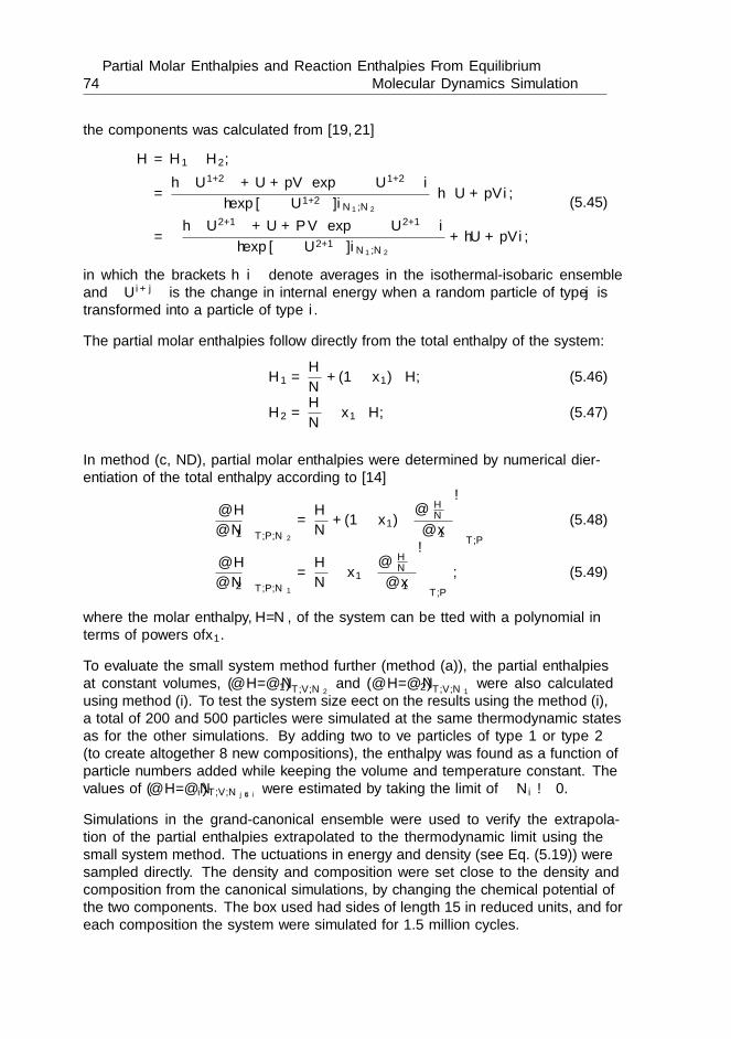
74Partial Molar Enthalpies and Reaction Enthalpies From Equilibrium
Molecular Dynamics Simulation
the components was calculated from [19,21]
∆H = H1 −H2,
=〈[∆U1+2− + U + pV
]exp
[−β∆U1+2−]〉
〈exp [−β∆U1+2−]〉N1,N2
− 〈U + pV 〉,
= −〈[∆U2+1− + U + PV
]exp
[−β∆U2+1−]〉
〈exp [−β∆U2+1−]〉N1,N2
+ 〈U + pV 〉,
(5.45)
in which the brackets 〈· · · 〉 denote averages in the isothermal-isobaric ensembleand ∆U i+j− is the change in internal energy when a random particle of type j istransformed into a particle of type i.
The partial molar enthalpies follow directly from the total enthalpy of the system:
H1 =H
N+ (1− x1)∆H, (5.46)
H2 =H
N− x1∆H, (5.47)
In method (c, ND), partial molar enthalpies were determined by numerical differ-entiation of the total enthalpy according to [14]
(∂H
∂N1
)
T,P,N2
=H
N+ (1− x1)
(∂(HN
)
∂x1
)
T,P
(5.48)
(∂H
∂N2
)
T,P,N1
=H
N− x1
(∂(HN
)
∂x1
)
T,P
, (5.49)
where the molar enthalpy, H/N , of the system can be fitted with a polynomial interms of powers of x1.
To evaluate the small system method further (method (a)), the partial enthalpiesat constant volumes, (∂H/∂N1)T,V,N2
and (∂H/∂N2)T,V,N1were also calculated
using method (i). To test the system size effect on the results using the method (i),a total of 200 and 500 particles were simulated at the same thermodynamic statesas for the other simulations. By adding two to five particles of type 1 or type 2(to create altogether 8 new compositions), the enthalpy was found as a function ofparticle numbers added while keeping the volume and temperature constant. Thevalues of (∂H/∂Ni)T,V,Nj 6=i were estimated by taking the limit of ∆Ni → 0.
Simulations in the grand-canonical ensemble were used to verify the extrapola-tion of the partial enthalpies extrapolated to the thermodynamic limit using thesmall system method. The fluctuations in energy and density (see Eq. (5.19)) weresampled directly. The density and composition were set close to the density andcomposition from the canonical simulations, by changing the chemical potential ofthe two components. The box used had sides of length 15 in reduced units, and foreach composition the system were simulated for 1.5 million cycles.
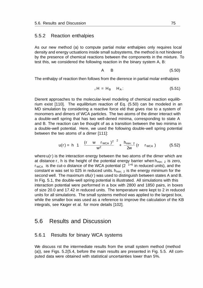
5.6. Results and Discussion 75
5.5.2 Reaction enthalpies
As our new method (a) to compute partial molar enthalpies only requires localdensity and energy fluctuations inside small subsystems, the method is not hinderedby the presence of chemical reactions between the components in the mixture. Totest this, we considered the following reaction in the binary system A, B:
A B (5.50)
The enthalpy of reaction then follows from the difference in partial molar enthalpies
∆rH = HB −HA. (5.51)
Different approaches to the molecular-level modeling of chemical reaction equilib-rium exist [110]. The equilibrium reaction of Eq. (5.50) can be modeled in anMD simulation by considering a reactive force field that gives rise to a system ofmonomers and dimers of WCA particles. The two atoms of the dimer interact witha double-well spring that has two well-defined minima, corresponding to state Aand B. The reaction can be thought of as a transition between the two minima ina double-well potential. Here, we used the following double-well spring potentialbetween the two atoms of a dimer [111]:
u(r) = h
[1− (r − w − rWCA)2
w2
]2
+hmin,2
2w(r − rWCA) (5.52)
where u(r) is the interaction energy between the two atoms of the dimer which areat distance r, h is the height of the potential energy barrier when hmin,2 is zero,rWCA is the cut-off distance of the WCA potential (21/6 in reduced units), and theconstant w was set to 0.25 in reduced units. hmin,2 is the energy minimum for thesecond well. The maximum of u(r) was used to distinguish between states A and B.In Fig. 5.1, the double-well spring potential is illustrated. All simulations with thisinteraction potential were performed in a box with 2800 and 1850 pairs, in boxesof size 20.0 and 17.42 in reduced units. The temperature were kept to 2 in reducedunits for all simulations. The small systems method was applied to the largest box,while the smaller box was used as a reference to improve the calculation of the KBintegrals, see Kruger et al. for more details [102].
5.6 Results and Discussion
5.6.1 Results for binary WCA systems
We discuss first the intermediate results from the small system method (method(a)), see Figs. 5.2–5.4, before the main results are presented in Fig. 5.5. All com-puted data were obtained with statistical uncertainties lower than 5%.
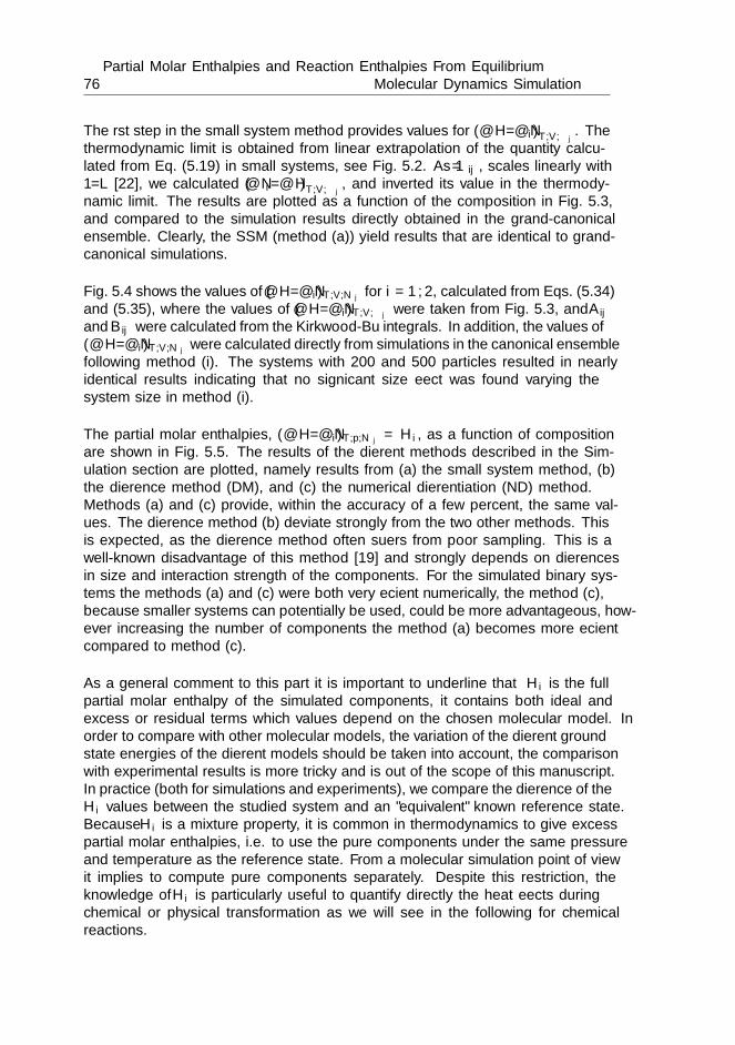
76Partial Molar Enthalpies and Reaction Enthalpies From Equilibrium
Molecular Dynamics Simulation
The first step in the small system method provides values for (∂H/∂Ni)T,V,µj . Thethermodynamic limit is obtained from linear extrapolation of the quantity calcu-lated from Eq. (5.19) in small systems, see Fig. 5.2. As 1/Γij , scales linearly with1/L [22], we calculated (∂Ni/∂H)T,V,µj , and inverted its value in the thermody-namic limit. The results are plotted as a function of the composition in Fig. 5.3,and compared to the simulation results directly obtained in the grand-canonicalensemble. Clearly, the SSM (method (a)) yield results that are identical to grand-canonical simulations.
Fig. 5.4 shows the values of (∂H/∂Ni)T,V,Nj for i = 1, 2, calculated from Eqs. (5.34)and (5.35), where the values of (∂H/∂Ni)T,V,µj were taken from Fig. 5.3, and Aijand Bij were calculated from the Kirkwood-Buff integrals. In addition, the values of(∂H/∂Ni)T,V,Nj were calculated directly from simulations in the canonical ensemblefollowing method (i). The systems with 200 and 500 particles resulted in nearlyidentical results indicating that no significant size effect was found varying thesystem size in method (i).
The partial molar enthalpies, (∂H/∂Ni)T,p,Nj = Hi, as a function of compositionare shown in Fig. 5.5. The results of the different methods described in the Sim-ulation section are plotted, namely results from (a) the small system method, (b)the difference method (DM), and (c) the numerical differentiation (ND) method.Methods (a) and (c) provide, within the accuracy of a few percent, the same val-ues. The difference method (b) deviate strongly from the two other methods. Thisis expected, as the difference method often suffers from poor sampling. This is awell-known disadvantage of this method [19] and strongly depends on differencesin size and interaction strength of the components. For the simulated binary sys-tems the methods (a) and (c) were both very efficient numerically, the method (c),because smaller systems can potentially be used, could be more advantageous, how-ever increasing the number of components the method (a) becomes more efficientcompared to method (c).
As a general comment to this part it is important to underline that Hi is the fullpartial molar enthalpy of the simulated components, it contains both ideal andexcess or residual terms which values depend on the chosen molecular model. Inorder to compare with other molecular models, the variation of the different groundstate energies of the different models should be taken into account, the comparisonwith experimental results is more tricky and is out of the scope of this manuscript.In practice (both for simulations and experiments), we compare the difference of theHi values between the studied system and an ”equivalent” known reference state.Because Hi is a mixture property, it is common in thermodynamics to give excesspartial molar enthalpies, i.e. to use the pure components under the same pressureand temperature as the reference state. From a molecular simulation point of viewit implies to compute pure components separately. Despite this restriction, theknowledge of Hi is particularly useful to quantify directly the heat effects duringchemical or physical transformation as we will see in the following for chemicalreactions.

5.6. Results and Discussion 77
5.6.2 Results for the reaction enthalpy
Just as for the SSM, method (b) requires one single simulation to compute partialmolar enthalpies. This is a clear advantage over method (c), which needs three ormore simulations in order to determine the enthalpy as a function of composition. Adrawback of method (b), mentioned already, is however the fact that the methodis unsuitable for particles which vary largely in size. Already for a system withWCA particles, this becomes evident. The small system method (a) can be usedto obtain partial molar enthalpies in a single simulation too. In the following, wewill apply the SSM to a reactive force field model for the reaction A B.
By keeping the parameters h and w in Eq. (5.52) constant, and by varying theparameter hmin,2, the effect of a difference in energy between the wells of thedumbbells was obtained. Based on Van’t Hoff equation and using the propertythat the number of A or B molecules are proportional to their potential energy, themole fraction of A and B can be written, in first approximation, as a function ofthe potential energy hmin,2:
xA =1
1 + J exp(−hmin,2kBT
) , (5.53)
xB =1
1 +[J exp
(−hmin,2kBT
)]−1 , (5.54)
where J is a constant which can be fitted to equilibrium results at a single temper-ature.
In Table 5.1, we present simulation results for the equilibrium mole fraction ofcomponents A, the threshold value (the maximum of the function u(r)), and thereaction enthalpy (∆rh). The results of xA calculated with Eq. (5.54) are in ex-cellent agreement with the values of the simulation under equilibrium chemicalconditions.
In Fig. 5.6, the computed reaction enthalpy, using our new method (a), is plotted asa function of the energy difference between the two wells in the dumbbell-potential,hmin,2. It is worth to note that ∆rS = ∆rH/T because the system obeys chemicalequilibrium. As expected for this simple system, the reaction enthalpy is linearlyproportional to the energy difference between components A and B, hmin,2, ∆rH =0.703 + 0.912hmin,2, the slope constant, 0.912, being close to one. As can be seenfrom Table 5.1, the composition of the system changes significantly with the valueof hmin,2 following Eq. (5.54).

78Partial Molar Enthalpies and Reaction Enthalpies From Equilibrium
Molecular Dynamics Simulation
5.7 Conclusions
We have presented a computational method for calculation of partial molar en-thalpies and reaction enthalpies for systems of interacting particles. The methodrequires simulations in the canonical ensemble or alternatively in the microcanon-ical or grand-canonical ensemble, and the sampling of energy and particle fluctu-ations inside small sub-systems. Using Kirkwood-Buff integrals, partial enthalpiesin the grand-canonical ensemble can be converted into partial enthalpies in thecanonical ensemble, as well as partial molar enthalpies in isobaric-isothermal en-semble.
The results of our method lead to the same results as obtained by differentiationof the enthalpy with respect to the composition. It can in addition be used todetermine partial molar enthalpies directly from a single canonical simulation.
The small system method has the significant advantage above the other methodsin its ability to handle the electroneutrality condition for ionic systems [56]. Wehave shown that the method can also be conveniently used to calculate reactionenthalpies in the context of a reactive force field model from a single MD simulation.
Acknowledgments
Computational resources were supported by NWO Exacte Wetenschappen (Physi-cal Sciences) for the use of supercomputer facilities, with financial support from theNederlandse Organisatie voor Wetenschappelijk Onderzoek (Netherlands Organi-zation for Scientific Research, NWO). SK, SKS, and TJHV acknowledge financialsupport through NWO-CW, through an ECHO grant. RS and SK acknowledgethe Storforsk grant no. 167336 from the Norwegian Research Council and theDepartment of Chemistry at the Norwegian University of Science and Technologyfor financing the PhD of RS. SKS also acknowledges financial support from theResearch Council of Norway through a Post-Doc. Fellowship, grant no. 230534.
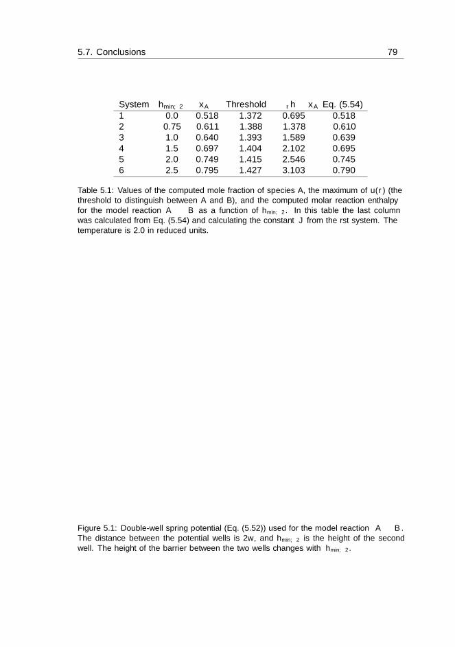
5.7. Conclusions 79
System hmin,2 xA Threshold ∆rh xA Eq. (5.54)1 0.0 0.518 1.372 0.695 0.5182 0.75 0.611 1.388 1.378 0.6103 1.0 0.640 1.393 1.589 0.6394 1.5 0.697 1.404 2.102 0.6955 2.0 0.749 1.415 2.546 0.7456 2.5 0.795 1.427 3.103 0.790
Table 5.1: Values of the computed mole fraction of species A, the maximum of u(r) (thethreshold to distinguish between A and B), and the computed molar reaction enthalpyfor the model reaction A B as a function of hmin,2. In this table the last columnwas calculated from Eq. (5.54) and calculating the constant J from the first system. Thetemperature is 2.0 in reduced units.
1.0 1.1 1.2 1.3 1.4 1.5 1.6 1.7 1.8ri
−2
−1
0
1
2
3
4
5
u dw(r
i)
2w
hmin,2
Figure 5.1: Double-well spring potential (Eq. (5.52)) used for the model reaction A B.The distance between the potential wells is 2w, and hmin,2 is the height of the secondwell. The height of the barrier between the two wells changes with hmin,2.
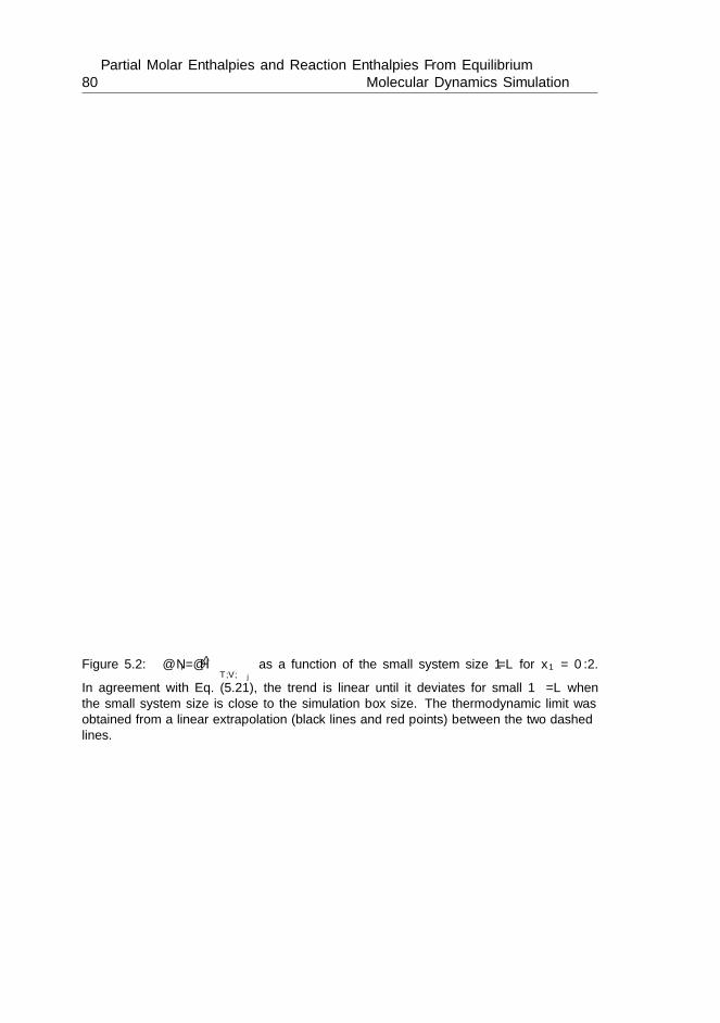
80Partial Molar Enthalpies and Reaction Enthalpies From Equilibrium
Molecular Dynamics Simulation
0.0 0.1 0.2 0.3 0.41/L [-]
0.05
0.10
0.15
0.20
0.25
0.30
0.35
0.40
( ∂Ni
∂H
) T,V,µ
j Component 1Component 2IntersectFitted line
Figure 5.2:(∂Ni/∂H
)T,V,µj
as a function of the small system size 1/L for x1 = 0.2.
In agreement with Eq. (5.21), the trend is linear until it deviates for small 1/L whenthe small system size is close to the simulation box size. The thermodynamic limit wasobtained from a linear extrapolation (black lines and red points) between the two dashedlines.
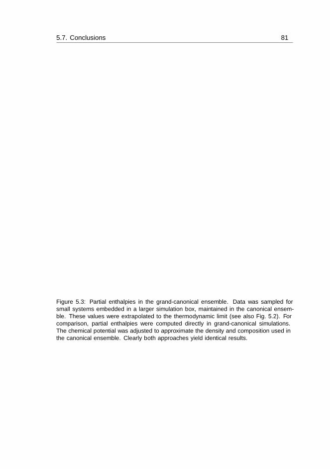
5.7. Conclusions 81
0.0 0.2 0.4 0.6 0.8 1.0x1
5
10
15
20
25
30
35
( ∂H ∂Ni) V
,T,µ
j
Component 1, SSMComponent 2, SSMComponent 1, µVTComponent 2, µVT
Figure 5.3: Partial enthalpies in the grand-canonical ensemble. Data was sampled forsmall systems embedded in a larger simulation box, maintained in the canonical ensem-ble. These values were extrapolated to the thermodynamic limit (see also Fig. 5.2). Forcomparison, partial enthalpies were computed directly in grand-canonical simulations.The chemical potential was adjusted to approximate the density and composition used inthe canonical ensemble. Clearly both approaches yield identical results.

82Partial Molar Enthalpies and Reaction Enthalpies From Equilibrium
Molecular Dynamics Simulation
0.0 0.2 0.4 0.6 0.8 1.0x1
5
10
15
20
25
30
35
40
( ∂H ∂N1
) V,T,N
2
NVT, Ntot = 200
NVT, Ntot = 500
Eq. 34
(a)
0.0 0.2 0.4 0.6 0.8 1.0x1
5
10
15
20
25
30
35
40
( ∂H ∂N2
) V,T,N
1
NVT, Ntot = 200
NVT, Ntot = 500
Eq. 35
(b)
Figure 5.4: Partial enthalpies in the NV T ensemble. A series of NV T simulations withdifferent particle numbers were carried out (method (i)). The red line is obtained byconverting the molar enthalpies from Fig. 5.3, using the Kirkwood-Buff coefficients neededto calculate A and B.
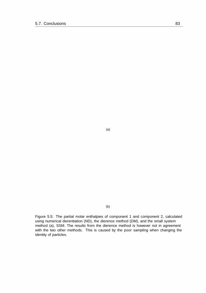
5.7. Conclusions 83
0.0 0.2 0.4 0.6 0.8 1.0x1
6
8
10
12
14
16
18( ∂H ∂N
1
) N2,
P,T
NDDMSSM
(a)
0.0 0.2 0.4 0.6 0.8 1.0x1
6
8
10
12
14
16
18
( ∂H ∂N2
) N1,
P,T
NDDMSSM
(b)
Figure 5.5: The partial molar enthalpies of component 1 and component 2, calculatedusing numerical differentiation (ND), the difference method (DM), and the small systemmethod (a), SSM. The results from the difference method is however not in agreementwith the two other methods. This is caused by the poor sampling when changing theidentity of particles.
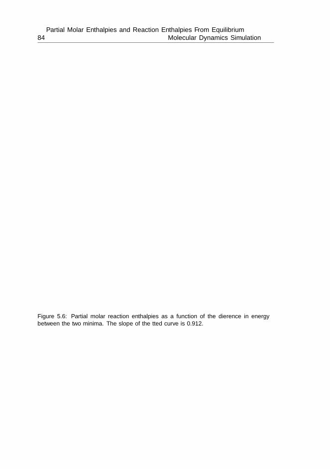
84Partial Molar Enthalpies and Reaction Enthalpies From Equilibrium
Molecular Dynamics Simulation
0.0 0.5 1.0 1.5 2.0 2.5hmin,2
0.5
1.0
1.5
2.0
2.5
3.0
3.5
∆ rh
SimulationLinear fit
Figure 5.6: Partial molar reaction enthalpies as a function of the difference in energybetween the two minima. The slope of the fitted curve is 0.912.

Chapter 6
The reaction enthalpy ofhydrogen dissociationcalculated with the SmallSystem Method fromsimulation of molecularfluctuations
Ragnhild Skorpa1, Jean-Marc Simon2, Dick Bedeaux1 andSigne Kjelstrup1,3
1. Department of Chemistry,Norwegian University of Science and Technology,
NO-7491 Trondheim, Norway
2. Laboratorie Interdisciplinaire Carnot de Bourgogne,UMR, CNRS-Universite de Bourgogne, Dijon, France.
3. Process & Energy Laboratory, Delft University of Technology,Leeghwaterstraat 39, 2628CB Delft, The Netherlands
This chapter was published in PCCP (2014) 16:19681–19693
86The reaction enthalpy of hydrogen dissociation calculated with the
Small System Method from simulation of molecular fluctuations
Abstract
We show how we can find the enthalpy of a chemical reaction under non-ideal con-ditions using the Small System Method to sample molecular dynamics simulationdata on fluctuating variables. This method, created with Hill’s thermodynamicanalysis, is used to find properties in the thermodynamic limit, such as thermo-dynamic correction factors, partial enthalpies, volumes, heat capacities and com-pressibility. The values in the thermodynamic limit at (T, V, µj), are then easilytransformed to other ensembles, (T, V,Nj) and (T, P,Nj), where the last ensemblegives the partial molar properties which are of interest to chemists. The dissociationof hydrogen from molecule to atoms was used as a convenient model system. Molec-ular dynamics simulations were preformed with three densities; ρ = 0.0052 g cm−3
(gas), ρ = 0.0191 g cm−3 (compressed gas) and ρ = 0.0695 g cm−3 (liquid), andtemperatures in the range; T = 3640 − 20800 K. The enthalpy of the reactionwas observed to follow a quadratic trend as a function of temperature for alldensities. The enthalpy of reaction was observed to only have a small pressuredependence. With a reference point close to an ideal stateA (T = 3640 K andρ = 0.0052 g cm−3), we where able to calculate the thermodynamic equilibriumconstant, and thus the distance from ideal conditions for the lowest density. Wefound the thermodynamic equilibrium constant to increase with increasing temper-ature, and with a negligible pressure dependence. Taking the enthalpy variationinto account in the calculation of the thermodynamic equilibrium constant, wefound the ratio of activity coefficients to be in the order of 0.7–1.0 for the lowestdensity, indicating repulsive forces between H and H2. The study shows that thecompressed gas- and liquid density at higher temperatures are far from ideal con-ditions. It is important to have a method that can give access to partial molarproperties, independent of the ideality of the reacting mixture. Our results showshow this can be achieved with the use of the Small System Method.
6.1 Introduction
It is cumbersome to obtain reliable values for enthalpies, in the laboratory as well asby computations [13]. Thanks to progress with a new molecular simulation method,the so-called Small System Method for prediction of thermodynamic data [22–24],one can now find precise values for partial molar enthalpies is a single simulation,from systematic studies of fluctuations in a small volume element [25]. The SmallSystem Method uses ideas first described by Hill [50], and the small system isembedded in a reservoir to examine the fluctuations in a small part under controlledconditions.
Molecular dynamics simulation have over the years been important for studiesof partial molar properties, such as enthalpy and volume as they determine theequilibrium properties of a multicomponent system. Kirkwood and Buff established
6.1. Introduction 87
already in 1951, a first fluctuation-based method for calculation of partial molarproperties from pair correlation functions [108]. Sindzingre et al. calculated thepartial molar enthalpy and -volume in terms of time averages [19, 112]. Shing andChung [113] calculated the partial molar volume and internal energy for an infinitelydilute system in 1988, and found them to be strongly dependent on the isothermalcompressibility. Debendetti used a fluctuation-based method to determine partialmolar volumes, energies and enthalpies [114–116]. Most of these methods do notgive the connection between the thermodynamic limit values for several ensembles,however, and the Small System Method may therefore offer an advantage.
Liu et al. have successfully used the method to find matrices of thermodynamicfactors, needed to relate Fick’s diffusion coefficients to Maxwell-Stefan diffusivities[54, 55]. The method was also used to find Kirkwood-Buff integrals, which arecentral for determination of thermodynamic properties in general (see e.g. BenNaim, [109]). Kirkwood-Buff integrals for closed systems are unable to deal withlinearly dependent variables [25], while this restriction is lifted in the Small SystemMethod, where the sampling takes place in a small, but open system. This is agreat advantage of the Small System Method [56], and it is therefore thought tobe particularly well suited for chemical reactions, as demonstrated by us for a toyreaction studied in [25]. This has given us the motivation to apply the method toa more realistic reaction.
The aim of this work is to determine the reaction enthalpy and related thermo-dynamic properties for a more realistic reaction, namely the hydrogen dissociationreaction. In earlier work [48] we established that the system of atoms and moleculescould be well modeled if the temperature was not too low (above 156 K). Usingthe dissociation constant based on mole fractions, Kx, and the van’t Hoff equation,we found an enthalpy of reaction equal to 430 kJ/mol in a dense fluid of the react-ing mixture. We shall now find the reaction enthalpy from a direct calculation ofpartial molar enthalpies and compare with that value.
The present work can be seen as an extension of the work by Xu and coworkerson chemical reactions [26, 31], but also of the Small System Method by Schnell etal. [22–24]. We shall present results for the compressibility, partial molar volumes,thermodynamic correction factors, and partial molar enthalpies of components ofthe hydrogen dissociation reaction. From this we find the reaction enthalpy and thetrue thermodynamic equilibrium constant. A classical description of the hydrogendissociation reaction has been established [48], producing a convenient basis forthe work. The hydrogen dissociation reaction is interesting e.g. in the physics ofplasma modeling [88, 117, 118]. In the chemical world it is relevant for separationof hydrogen gas from a gas mixture (e.g. from the water gas shift reaction) usinga palladium membrane [11, 64, 72]. At the surface of this membrane, molecularhydrogen dissociates and atomic hydrogen diffuses through the membrane and isrecombined to molecular hydrogen at the opposite surface [11,68,72].
The paper is structured as follows. In Section 6.2 we give a short recapitulationof the Small System Method. A description of the interaction potential and the
88The reaction enthalpy of hydrogen dissociation calculated with the
Small System Method from simulation of molecular fluctuations
simulation- and calculation procedures follow. Section 6.3 gives results, and finallywe give conclusions in Section 6.4.
6.2 Methods
6.2.1 The Small System Method
The Small System Method is used here to give access to partial enthalpies in thethermodynamic limit for a binary system, but the method can also be generalized.The enthalpies were first calculated for small systems at constant (T, V, µj). Aftergoing to the thermodynamic limit, the Small System Method, by Schnell et al. [25]gives the procedure to transform the variables to other ensembles. The expressionsfor these transformations between sets of partial enthalpies for two components iand j from (T, V, µj) to (T, V,Nj) is given in Eqs. (6.1) and (6.2)
(∂H
∂Ni
)
T,V,Nj 6=i
=Bjj
[Ajj
(∂H
∂Ni
)
T,V,µj 6=i
+Aij
(∂H
∂Nj
)
T,V,µi6=j
](6.1)
(∂H
∂Nj
)
T,V,Ni6=j
=Bii
[Aii
(∂H
∂Nj
)
T,V,µi6=j
+Aij
(∂H
∂Ni
)
T,V,µj 6=i
](6.2)
and then to (T, P,Nj)
(∂H
∂Ni
)
T,P,Nj 6=i
=ViH
V+NjV
[Vj
(∂H
∂Ni
)
T,V,Nj 6=i
− Vi(∂H
∂Nj
)
T,V,Ni6=j
](6.3)
with the last expression as the present target. In Eqs. (6.1) and (6.2) a summa-tion is performed over all double appearing indices.The expressions requires thethermodynamic limit value of:
• Partial enthalpies at constant T, V, µ
• Thermodynamic correction factors, Γij at T, V, µ (see Eq.(6.4))
• Partial molar volumes, Vi at constant T, V, µ
• Matrices Aij and Bij as defined by Kirkwood and Buff [108]
The input quantities are defined and briefly explained in the following subsectionsfor a binary mixture. For further details, see [25].
Partial enthalpies
The partial enthalpy of component i, hi, at constant T, V, µj is determined fromfollowing formula for fluctuations of the total energy and density in the small system
6.2. Methods 89
[25]
hi(L) =
(∂H
∂Ni
)
T,V,µj 6=i
= −〈UNi〉 − 〈U〉〈Ni〉+ kBT 〈Ni〉〈N2
i 〉 − 〈Ni〉2(6.4)
Brackets denote time averages. The Small System Method gives the enthalpy asa (predominantly) linear function of the inverse of the radius of the small sys-tem used in the sampling of fluctuation [22–24], L. The derivative of H (in thethermodynamic limit) is found by extrapolation.
hi(L) = hi,∞ +A′iL
+ ... (6.5)
Here, hi,∞ is the derivative of H at constant (T, V, µj) in the thermodynamic limit(needed in Eqs.(6.1) – (6.3)). For a spherical sampling volume, the scaling law onlyhas the linear term, as the non linear terms can be neglected [22].
Thermodynamic correction factor
The thermodynamic correction factor, Γij , is defined as
Γ−1ij =
1
β
(∂ln 〈Ni〉∂µj
)
T,V,µk 6=i
=1
β〈Ni〉
(∂〈Ni〉∂µj
)
T,V,µk 6=i
(6.6)
where β = 1/kBT , kB is Boltzmann’s constant, µ is the chemical potential andsubscript i or j denote H or H2. At constant (T, V, µj) we determine Γij from thefluctuation theory formula derived by Reed and Ehrlich [119].
Γ−1ij (L) =
〈NiNj〉 − 〈Ni〉〈Nj〉〈Nj〉
(6.7)
The Small System Method gives the inverse of the thermodynamic correction fac-tor as a (predominantly) linear function of the inverse of L [22–24] for constant(T, V, µj):
Γ−1ij (L) = Γ−1
ij,∞ +AijL
+ .... (6.8)
We use this to obtain Γ−1ij,∞ in the thermodynamic limit as a function of T, V, µj .
In the following sections the values in the thermodynamic limit is used.
Kirkwood-Buff integrals and the matrices Aij , Bij
The integral over the pair correlation function gij of the particle fluctuations, iscalled the Kirkwood-Buff integral after the groundbreaking work of Kirkwood andBuff [108]
Gij =
∫[gij(r)− 1]dV = V
〈NiNj〉 − 〈Ni〉〈Nj〉〈Ni〉〈Nj〉
− δijci
=1
ciΓ−1ij −
δijci
(6.9)
90The reaction enthalpy of hydrogen dissociation calculated with the
Small System Method from simulation of molecular fluctuations
where Gij is the Kirkwood-Buff integral at constant T, V, µj , δ is the Kroeneckerdelta, and ci is the concentration of i (ci = Ni/V ). The last equality in Eq.(6.9)was obtained by introducing Eq.(6.7) in the middle equality of Eq (6.9). Note thatGij and (1/ci)Γ
−1ij are symmetric. Several properties can be expressed by these
integrals, such as partial molar volume and isothermal compressibility. Both thethermodynamic limit value of Gij and Γ−1
ij,∞ are as a function of (T, V, µj).
Following Kirkwood and Buff [108] or more transparently Ben Naim [109] (Eqs.4.23 and 4.24), we have for the symmetric Bij matrix, at constant (T, V, µj)
Bij = Bji =kBT
V
(∂Nj∂µi
)
T,V,µk 6=i
= kBT
(∂cj∂µi
)
T,V,µk 6=i
(6.10)
= cicjGij + ciδij =1
V(〈NiNj〉 − 〈Ni〉 〈Nj〉)
where Gij always are Kirkwood-Buff integrals which refer to the grand canonicalensemble. Furthermore we define the matrix Aij , at constant T, V,Nj , by
Aij = Aji = βV
(∂µj∂Ni
)
T,V,Nk 6=i
= β
(∂µj∂ci
)
T,V,ck 6=i
(6.11)
The Aij and Bij matrices are each other’s inverse, so:∑
j
BijAjk = δik (6.12)
These properties can be used to characterize a binary reacting mixture, as we shallsee.
Properties from the Kirkwood-Buff integrals
Kirkwood and Buff gave the derivative of the chemical potential of one componentwith respect to its mole fraction in a binary mixture, at constant T and P
1
kBT
(∂µi∂xi
)
T,P
=1
xi+
cj (2Gij −Gii −Gjj)1 + xicj (Gii +Gjj − 2Gij)
(6.13)
where xi is the mole fraction of i (xi = Ni/(NH +NH2); here NH2
is the number ofmolecules so that xH +xH2
= 1). The relation between the thermodynamic correc-tion factor and the activity coefficient, γi, was also given in terms of Kirkwood-Buffintegrals [23] (
∂ln γi∂lnxi
)
T,P
= − xicj(Gii +Gjj − 2Gij)
1 + cjxi(Gii +Gjj − 2Gij(6.14)
The partial molar volume (Eq.(6.15)) and the isothermal compressibility (Eq.(6.16))for a binary mixture are
Vi =1 + (Gjj −Gij)cj
ci + cj + cicj(Gii +Gjj − 2Gij)(6.15)
6.2. Methods 91
and
κkBT =1 +Giici +Gjjcj +
(GiiGjj −G2
ij
)cicj
ci + cj + (Gii +Gjj − 2Gij) cicj(6.16)
Thermodynamic properties of the chemical reaction
The enthalpy of a system is H = U +PV , where U is the internal energy, P is thepressure, and V is the volume. The enthalpy at constant T and P can be writtenas
H =
n∑
i=1
HiNi (6.17)
where Hi is the partial molar enthalpy of component H or H2. Thus, the partialmolar enthalpy is the derivative of H with respect to the number of either H orH2, Ni:
Hi =
(∂H
∂Ni
)
T,P,Nj
(6.18)
The enthalpy of a reaction is given by the partial molar enthalpies of the compo-nents
∆rH = 2HH −HH2(6.19)
The equilibrium constant can be calculated from the van’t Hoff equation, at con-stant pressure, if the enthalpy of reaction is known at standard conditions.
[d(lnKth)
d(1/T )
]
P
= −∆rH
R(6.20)
Superscript denotes the standard state (1 bar). In the presence of a varyingpressure, there is an additional term in this equation:
d lnKth = −∆rH
Rd
(1
T
)− ∆rV
RTdP (6.21)
where the last term gives the pressure dependence, and ∆rV is the reaction
volume.
With ideal gas and pure component as standard state at 1 bar pressure, the chemicalpotential is
µi = µi +RT ln fi/P
= µ +RT ln(xiPγi)/P (6.22)
The fugacity of the gas component, fi, is equal to the partial pressure of the gas,which is xiP , times the activity coefficient γi. By introducing this into the condition∆G = 0 for the reaction in question we obtain the equilibrium constant in termsof the dissociation constant, Kx, total pressure, and the activity coefficient ratio:
Kth =x2
H
xH2
P
Pγ2
H
γH2
= KxP
Pγ2
H
γH2
= KPγ2
H
γH2
(6.23)

92The reaction enthalpy of hydrogen dissociation calculated with the
Small System Method from simulation of molecular fluctuations
where KP = KxP/P is the pressure based dissociation constant. The partial
molar heat capacities of the components and the reaction and the isothermal com-pressibility of the mixture are found from standard expressions:
CP =
(∂H
∂T
)
P
(6.24)
κT = − 1
V
[∂V
∂P
]
T
(6.25)
The ideal value of the heat capacity of the reaction is 3R/2, when vibrational modesare not excited. For an ideal gas, κT = 1/P .
The temperature T is calculated from the average kinetic energy per degree offreedom of all particles:
T =1
3kBNp
Np∑
i=1
miv2i (6.26)
where v2i = v2
x,i+ v2y,i+ v2
z,i and Np = NH + 2NH2 is the total number of atoms.
From the virial theorem, the expression for the pressure in the presence of two- andthree-particle interactions is:
P =kBTNpV
− 1
3V
Np∑
i=1
1
2
∑
j pair with i
∂u2(rij)
∂rijrij (6.27)
+∑
j<k triplet with i
(∂hj,i,k(rji, rik, θj,i,k)
∂rjirji
+∂hj,i,k(rji, rik, θj,i,k)
∂rikrik +
∂hj,i,k(rji, rik, θj,i,k)
∂rjkrjk
)]
The first term in Eq. (6.27) gives the ideal contribution to the pressure, whilethe second term gives the contribution from the two- and three particle potentials,respectively. For a discussion regarding the pressure calculations, see [48].
6.2.2 Interaction Potentials
The chemical reaction was modeled accurately with molecular dynamics simulationsusing anaytical potentials derived from quantum mechanical results, in the samemanner as [3,26,29,31]. Stillinger and Weber [3] showed that it was sufficient to usean interaction potential, U , which is the sum of two- and three-particle interactioncontributions, to describe the essentials of a chemical reaction:
U(r1, ..., rN ) =∑
i<j
u(2)(rij) +∑
i<j<k
u(3)(ri, rj , rk) (6.28)

6.2. Methods 93
here u(2) and u(3) are the two- and three-particle potentials, given in Eqs. (6.29)and (6.30), respectively. Based on the quantum mechanical results of Diedrichand Anderson [46, 47], Kohen et al derived expressions for two- and three-particlepotentials [29] for hydrogen.
u(2)(r) =
{α (β2r
−p − 1) exp[
γ2r−rc
]if r < rc
0 if r > rc(6.29)
here α = 5.59 · 10−21 kJ, β2 = 0.044067 Ap, γ2 = 3.902767 A, rc = 2.8 A and p = 4are constants [29]. α is chosen such that the minimum of the potential gives thebinding energy of hydrogen (432.065 kJ mol−1) [29] at the bond distance between
two hydrogen atoms, re = 0.74 A [47]. When the distance between two atoms islarger than the cut-off distance, r ≥ rc, the potential is zero. Reduced units, basedon the pair potential, are used throughout the paper. σ is defined at u2(σ) = 0,
giving σ = p√β2 = 0.458A, and ε is based on the binding energy of hydrogen, so
that −ε is the minimum of the pair potential, giving ε/kB = 51991 K.
The three particle-potential is given as a sum over the contribution from each par-ticle, and it’s role is to prevent formation of more than one bond to each hydrogenatom.
u(3) = hi,j,k(rij , rjk, θi,j,k) + hj,i,k(rji, rik, θj,i,k) + hi,k,j(rik, rkj , θi,k,j) (6.30)
Where the h-functions are given by
hj,i,k(rji, rik, θj,i,k) =
{λa exp
[γ3
(rji−rc) + γ3(rik−rc)
]if rji < rc and rik < rc
0 otherwise(6.31)
anda =
[1 + µ cos(θj,i,k) + ν cos2(θj,i,k)
](6.32)
λ = 2.80 · 10−21 kJ, µ = 0.132587, ν = −0.2997 and γ3 = 1.5 A are constants [29].The cut-off distance, rc, is the same for both the two- and three-particle interactions(2.8 A). The interaction potential we use has a finite range (has no long rangedispersion attraction). A potential tail plays no role for the chemical reaction.
In the triad subscript j, i, k the middle letter i refers to the atom at the subtendedangle vertex. A full description and analysis of the interaction potential was givenearlier [48]. The total potential was used to determine the distance of chemicallybonded particles. When the distance between two particles was shorter than r∗ji ≤4.0, they were labeled as part of a molecule, in agreement with the procedure usedby Stillinger and Weber [3].
6.2.3 Calculation details
The simulation procedure was given earlier [48], and for this reason only the maindetails are given here. The simulation box contained 1000 particles (Np = NH +

94The reaction enthalpy of hydrogen dissociation calculated with the
Small System Method from simulation of molecular fluctuations
2NH2 = 1000), with dimensions V = LxLyLz, where Ly = Lz = Lx/2. The mass ofone hydrogen atom, m0 = 1.67 ·10−27 kg, was used to define the reduced total massdensity ρ∗ = ρσ3/m0. This implies that the reduced total mass density equals thereduced total molar density in terms of (Np = NH +2NH2
). Reduced units are usedthroughout the paper, and are indicated by superscript ∗. The relations betweenreal and reduced units is given in Table 6.1, ε/kB = 51991 K and σ = 0.458 A [48].
Table 6.1: Relations between reduced and real units, ε/kB = 51991 K, σ=0.458 A andm0 = 1.67 · 10−27 kg.
Reduced variables FormulaMass m∗ = m/m0
Distance r∗ = r/σEnergy u∗ = u/ε
Time t∗ = (t/σ)√ε/m0
Temperature T ∗ = kBT/εDensity ρ∗ = ρσ3/m0
Pressure P ∗ = Pσ3/ε
Velocity v∗ =v√m0/ε
Dissociation of H2
The degree of dissociation, mole fraction and pressure for the two higher densitieswas studied by us in a previous paper [48]. These results are repeated here for easeof reading, and supplemented with similar results for the low density ρ∗ = 0.0003,see Tables 6.2–6.4.
For the lowest gas-like density, ρ∗ = 0.0003 in Table 6.2, we have almost 1 % dis-sociation at the lowest temperature (T ∗ = 0.07), while for the highest temperature(T ∗ = 0.4) we have almost 80 % dissociation.
Table 6.2: Number of H atoms (NH), mole fraction (xi), total pressure (P ∗) and thedissociation constant (Kx) for the density, ρ∗ = 0.0003.
T ∗ 0.07 0.15 0.2 0.25 0.3 0.4NH 8 254.17 477.81 574.69 710.95 760.95NH2
496 372.92 261.09 212.65 144.52 119.52xH2 0.984 0.595 0.353 0.270 0.169 0.136Kx - 0.276 1.183 1.973 4.088 5.502105P ∗ 1.138 3.045 4.672 6.347 7.983 11.148
By increasing the density to that of a denser gas, to ρ∗ = 0.0011 in Table 6.3, thedissociation degree decreases as expected. It is less than 1 % at T ∗ = 0.07, and

6.2. Methods 95
about 55 % at T ∗ = 0.4.
Table 6.3: Number of H atoms (NH), mole fraction (xi), total pressure (P ∗) and thedissociation constant (Kx) for the density, ρ∗ = 0.0011.
T ∗ 0.07 0.15 0.2 0.25 0.3 0.4NH 5.92 147.71 285.00 396.19 468.74 554.88NH2
497.04 426.14 357.50 301.91 265.63 227.56xH2 0.988 0.743 0.556 0.432 0.362 0.295Kx - 0.089 0.354 0.745 1.126 1.689105P ∗ 5.082 12.119 17.554 23.287 29.054 40.492
At the highest (liquid-like) density, ρ∗ = 0.004 in Table 6.4, a further decrease isseen in the degree of dissociation. For the lowest temperature, T ∗ = 0.07, we nowhave 0.2 % dissociation, while there is an increase to 29 % for T ∗ = 0.4.
Table 6.4: Number of H atoms (NH), mole fraction (xi), total pressure (P ∗) and thedissociation constant (Kx) for the density, ρ∗ = 0.004.
T ∗ 0.07 0.15 0.2 0.25 0.3 0.4NH 1.98 66.90 137.61 192.39 232.42 288.50NH2
499.01 466.55 431.19 403.81 383.79 355.75xH2 0.996 0.875 0.758 0.677 0.623 0.552Kx - 0.018 0.077 0.154 0.228 0.363104P ∗ 4.094 8.478 11.292 14.051 16.729 21.892
Simulations were carried out for the series of composition and temperature listedin these tables, and thermodynamic data were computed according to this and theequations given in Section 2.1.
Simulation details
The Small System Method was applied according to procedures described by Schnellet al. [22–25], using the formulas given in Section 2.1. The sampling volume was asphere with radius, L, varying from L = σ to L = 0.5Ly, where Ly is the length ofthe simulation box in the y-direction. The sampling was done at random positionsin the simulation box. The number of particles and the energy were then computedfor each sphere (50 spheres per sampling) and the time average gave the fluctua-tion of particle numbers and energy. The fluctuations were sampled every 100 timestep, and time averages were calculated every 10 000 time step, after equilibrationof the system. Data was plotted as a function of 1/L. In order to test reservoir sizedependence, we repeated some of the equilibrium simulations for the same densitywith 4096 particles, no significant size dependence was observed.
96The reaction enthalpy of hydrogen dissociation calculated with the
Small System Method from simulation of molecular fluctuations
To check that the method performed in the expected way, we plotted the thermo-dynamic correction factors, obtained from particle fluctuations, versus the inversesphere size (1/L). The plots are given in Figure 6.1 for T ∗ = 0.07, for all densities(ρ∗ = 0.0003, ρ∗ = 0.0011 and ρ∗ = 0.004).
For the lowest density ρ∗ = 0.0003 in Figure 6.1(a), we see that Γ−1HH as well as Γ−1
HH2
vary linearly with 1/L. The linear regression was in all cases done for points in theregion 0.125 ≤ 1/L∗ ≤ 0.16, a range where such a dependence was observed. Therange corresponded to spheres that included from 12 to 16 particles. It was chosenafter observing that the inverse thermodynamic correction factor for systems with4096 and 1000 particles coincide in this range.
The values reported are as expected. When the radius of the small system ap-proaches zero, the value of Γ−1
ii approaches 1, as a volume with one particle isideal. The value of Γ−1
HH = 1 obeys this already for a wide range of values, whileΓ−1
H2H2increases from approximately 0.9 for the biggest sphere to 1 for 1/L = 0.4
The correlation between H and H2 is approximately zero, as the system mainlycontains H2, explaining Γ−1
HH2 = 0.
The results for the higher densities followed the same trend. By increasing thedensity to ρ∗ = 0.0011, see Figure 6.1(b), we find again that Γ−1
HH and Γ−1H2H2
are constant, while the Γ−1H2H2
increases with decreasing size of the sphere, and at1/L = 0.5 we see that it is approximately 1. For the highest density, ρ∗ = 0.004in Figure 6.1(c), we again see that Γ−1
HH is approximately 1 and independent of thesizes of the spheres, while Γ−1
H2H2increases towards 1 for small spheres as expected.
For all three densities, there is only a variation in the value of Γ−1H2H2
. For alldensities the factor increases with decreasing size of the sphere, and we also seethat by increasing the density (and the number of H2) we decrease the value in thethermodynamic limit. The limiting value of 1 for infinitely small spheres is reachedfor all densities, the approach being faster for the lowest density. Γ−1
HH and Γ−1HH2
are constant at 1 and 0, respectively, for all densities.
All these results on Γ−1ij (L) taken together confirm that the method works in a
manner expected for the thermodynamic correction factor for the range of thevariables chosen. This range is well above the limit where quantum mechanicaleffects take over [48], and away from boundaries where singularities can be expected[25]. We are therefore confident about the results.
No further results will be shown for Γij(L), as the smallness of the system isnot a topic per se. We present results which all have been extrapolated to thethermodynamic limit.
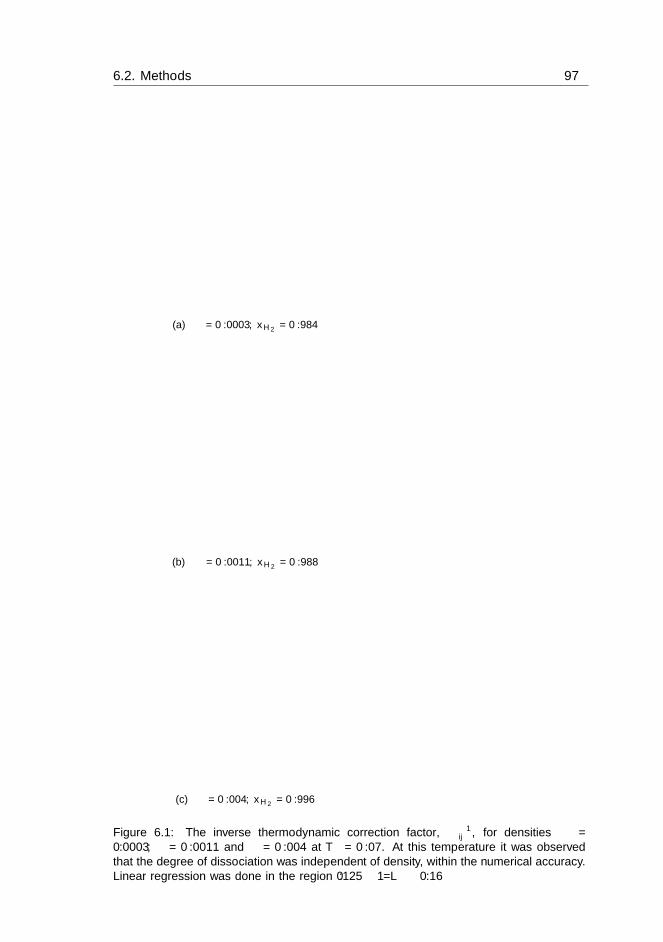
6.2. Methods 97
-0.4
-0.2
0
0.2
0.4
0.6
0.8
1
0 0.1 0.2 0.3 0.4 0.5
Γ ij-1
1/L*
H-HH2-H2H-H2
(a) ρ∗ = 0.0003, xH2= 0.984
-0.4
-0.2
0
0.2
0.4
0.6
0.8
1
0 0.1 0.2 0.3 0.4 0.5
Γ ij-1
1/L*
H-HH2-H2H-H2
(b) ρ∗ = 0.0011, xH2= 0.988
-0.4
-0.2
0
0.2
0.4
0.6
0.8
1
0 0.1 0.2 0.3 0.4 0.5
Γ ij-1
1/L*
H-HH2-H2H-H2
(c) ρ∗ = 0.004, xH2 = 0.996
Figure 6.1: The inverse thermodynamic correction factor, Γ−1ij , for densities ρ∗ =
0.0003, ρ∗ = 0.0011 and ρ∗ = 0.004 at T ∗ = 0.07. At this temperature it was observedthat the degree of dissociation was independent of density, within the numerical accuracy.Linear regression was done in the region 0.125 ≤ 1/L∗ ≤ 0.16

98The reaction enthalpy of hydrogen dissociation calculated with the
Small System Method from simulation of molecular fluctuations
6.3 Results
The main outcome of the calculations are the sets of enthalpies at constant (T, V, µj),(T, V,Nj) and (T, P,Nj), and the results derived from them. We present first theenthalpies obtained for the thermodynamic limit in the ensemble (T, V, µj), theoriginal data from the sampling of fluctuations in the small system, and the cor-responding sets for other ensembles, obtained by Lagrange transformations, seeEqs.(6.1) and (6.2).
The matrices Aij and Bij are not directly reported, instead we give Γ−1ij which is
equivalent to Bij , and which gives Aij . The temperature interval T ∗ = 0.07− 0.4was used. We proceed to present results for the partial enthalpies in the differentensembles, the thermodynamic correction factors, the partial molar volumes, andthe isothermal compressibility, to elucidate system properties, before we determinethe enthalpy of reaction and the equilibrium constant as a function of temperature.
6.3.1 Partial molar enthalpy
The partial enthalpy at constant (T, V, µj), h, was found using the fluctuationmethod described in Section 6.2.3 for T ∗ = 0.7 − 0.4. The results for h for Hand H2 (for the small system) are shown as a function of the inverse radius of thesmall system in Figure 6.2 for T ∗ = 0.2. At this temperature, the mole fraction ofH2 varies from xH2
= 0.353 (ρ∗ = 0.0003) to xH2= 0.758 (ρ∗ = 0.004) between
the lowest and highest densities. The linear regression was preformed in the range0.15 ≤ 1/L∗ ≤ 0.3. The range was chosen after comparing results for systemswith with 1000 and 4096 particles. No size effect was found in this range. At theother temperatures, the plots looked like Figures 6.2(a) and 6.2(b), and are for thisreason not shown.
The extrapolated partial enthalpies in the thermodynamic limit are given in Table6.5 for all temperatures, T ∗ = 0.07−0.4, and all densities; ρ∗ = 0.0003, ρ∗ = 0.0011and ρ∗ = 0.004. All results showed a linear dependence and the linear regressionwas done for 0.15 ≤ 1/L∗ ≥ 0.3 in all cases.
From Table 6.5 we see that the partial enthalpy increases with increasing temper-ature, for H as well as H2, for all densities. Using the method by Schnell et al. [25]we transformed the partial enthalpies at (∂H∗/∂Ni)T,V,µj 6=i to (∂H∗/∂Ni)T,V,Nj 6=iand finally to the partial molar enthalpies, (∂H∗/∂Ni)T,P,Nj 6=i . Where the partialmolar enthalpies gives us access to the reaction enthalpy of the system as a functionof the temperature, independent of the ideality of the mixture.
A plot of the data in Table 6.5 partial enthalpies in the different ensembles;(T, V, µj), (T, V,Nj) and (T, P,Nj) is given in Figure 6.3. The results for the differ-ent conditions may be interesting for a set of application purposes. Additional dataare added in the plot for the highest densities, ρ∗ = 0.0011 and ρ∗ = 0.004. The

6.3. Results 99
0.55
0.6
0.65
0.7
0.75
0.8
0.85
0 0.1 0.2 0.3 0.4 0.5
hi
1/L*
HH2
(a) ρ∗ = 0.0003, xH2= 0.353
0.55
0.6
0.65
0.7
0.75
0.8
0.85
0 0.1 0.2 0.3 0.4 0.5
hi
1/L*
HH2
(b) ρ∗ = 0.0011, xH2= 0.556
0.55
0.6
0.65
0.7
0.75
0.8
0.85
0 0.1 0.2 0.3 0.4 0.5
hi
1/L*
HH2
(c) ρ∗ = 0.004, xH2 = 0.758
Figure 6.2: Partial enthalpies determined from fluctuation at (T, V, µj), hi, as a functionof the size of the sphere (1/L∗) at T ∗ = 0.2. The linear regression was done in the region0.15 ≤ 1/L∗ ≤ 0.3.
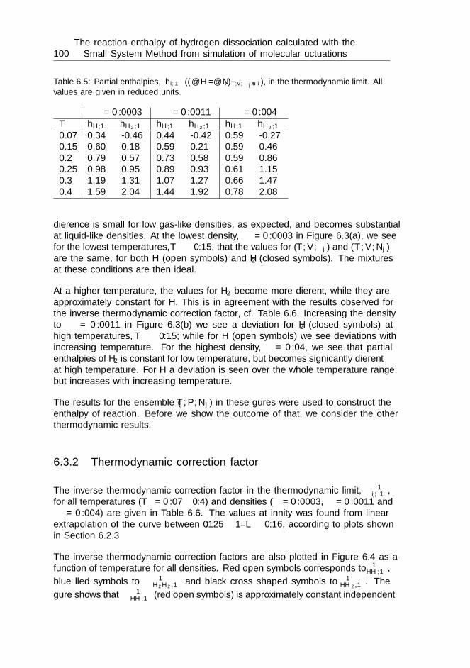
100The reaction enthalpy of hydrogen dissociation calculated with the
Small System Method from simulation of molecular fluctuations
Table 6.5: Partial enthalpies, hi,∞ ((∂H∗/∂Ni)T,V,µj 6=i), in the thermodynamic limit. Allvalues are given in reduced units.
ρ∗ = 0.0003 ρ∗ = 0.0011 ρ∗ = 0.004T ∗ hH,∞ hH2,∞ hH,∞ hH2,∞ hH,∞ hH2,∞0.07 0.34 -0.46 0.44 -0.42 0.59 -0.270.15 0.60 0.18 0.59 0.21 0.59 0.460.2 0.79 0.57 0.73 0.58 0.59 0.860.25 0.98 0.95 0.89 0.93 0.61 1.150.3 1.19 1.31 1.07 1.27 0.66 1.470.4 1.59 2.04 1.44 1.92 0.78 2.08
difference is small for low gas-like densities, as expected, and becomes substantialat liquid-like densities. At the lowest density, ρ∗ = 0.0003 in Figure 6.3(a), we seefor the lowest temperatures, T ∗ ≤ 0.15, that the values for (T, V, µj) and (T, V,Nj)are the same, for both H (open symbols) and H2 (closed symbols). The mixturesat these conditions are then ideal.
At a higher temperature, the values for H2 become more different, while they areapproximately constant for H. This is in agreement with the results observed forthe inverse thermodynamic correction factor, cf. Table 6.6. Increasing the densityto ρ∗ = 0.0011 in Figure 6.3(b) we see a deviation for H2 (closed symbols) athigh temperatures, T ∗ ≥ 0.15; while for H (open symbols) we see deviations withincreasing temperature. For the highest density, ρ∗ = 0.04, we see that partialenthalpies of H2 is constant for low temperature, but becomes significantly differentat high temperature. For H a deviation is seen over the whole temperature range,but increases with increasing temperature.
The results for the ensemble (T, P,Nj) in these figures were used to construct theenthalpy of reaction. Before we show the outcome of that, we consider the otherthermodynamic results.
6.3.2 Thermodynamic correction factor
The inverse thermodynamic correction factor in the thermodynamic limit, Γ−1ij,∞,
for all temperatures (T ∗ = 0.07− 0.4) and densities (ρ∗ = 0.0003, ρ∗ = 0.0011 andρ∗ = 0.004) are given in Table 6.6. The values at infinity was found from linearextrapolation of the curve between 0.125 ≤ 1/L ≤ 0.16, according to plots shownin Section 6.2.3
The inverse thermodynamic correction factors are also plotted in Figure 6.4 as afunction of temperature for all densities. Red open symbols corresponds to Γ−1
HH,∞,
blue filled symbols to Γ−1H2H2,∞ and black cross shaped symbols to Γ−1
HH2,∞. The
figure shows that Γ−1HH,∞ (red open symbols) is approximately constant independent

6.3. Results 101
-0.5
0
0.5
1
1.5
2
2.5
3
3.5
4
0.05 0.1 0.15 0.2 0.25 0.3 0.35 0.4
(δH
* /δN
i)
T*
(δH*/δNH)T,V,µH2
(δH*/δNH)T,V,NH2
(δH*/δNH)T,P,NH2
(δH*/δNH2)T,V,µH
(δH*/δNH2)T,V,NH
(δH*/δNH2)T,P,NH
(a) ρ∗ = 0.0003
-0.5
0
0.5
1
1.5
2
2.5
3
3.5
4
0.05 0.1 0.15 0.2 0.25 0.3 0.35 0.4
(δH
* /δN
i)
T*
(δH*/δNH)T,V,µH2(δH*/δNH)T,V,NH2(δH*/δNH)T,P,NH2(δH*/δNH2
)T,V,µH(δH*/δNH2
)T,V,NH(δH*/δNH2
)T,P,NH
(b) ρ∗ = 0.0011
0
1
2
3
4
0.05 0.1 0.15 0.2 0.25 0.3 0.35 0.4
(δH
* /δN
i)
T*
(δH*/δNH)T,V,µH2(δH*/δNH)T,V,NH2(δH*/δNH)T,P,NH2(δH*/δNH2
)T,V,µH(δH*/δNH2
)T,V,NH(δH*/δNH2
)T,P,NH
(c) ρ∗ = 0.004
Figure 6.3: Partial enthalpies for all densities at the different ensembles; T, V, µj (�),T, V,Nj (◦) and T, P,Nj (4). Open symbols corresponds to values for H while closedsymbols represent H2.

102The reaction enthalpy of hydrogen dissociation calculated with the
Small System Method from simulation of molecular fluctuations
Table 6.6: The inverse thermodynamic correction factors, Γ−1ij,∞, at constant µ, V, T in the
thermodynamic limit.
ρ∗ = 0.0003 ρ∗ = 0.0011
T ∗ Γ−1HH,∞ Γ−1
HH2,∞ Γ−1H2H2,∞ Γ−1
HH,∞ Γ−1HH2,∞ Γ−1
H2H2,∞0.07 1.00 -0.00 0.87 1.01 -0.00 0.600.15 1.00 -0.04 0.91 0.98 -0.08 0.670.2 0.98 -0.08 0.94 0.97 -0.16 0.730.25 0.96 -0.09 0.97 0.93 -0.20 0.780.3 0.96 -0.12 0.97 0.91 -0.24 0.820.4 0.94 -0.11 0.99 0.88 -0.28 0.87
ρ∗ = 0.004
T ∗ Γ−1HH,∞ Γ−1
HH2,∞ Γ−1H2H2,∞
0.07 1.01 -0.00 0.130.15 1.02 -0.07 0.210.2 0.97 -0.17 0.230.25 0.97 -0.22 0.340.3 0.95 -0.26 0.380.4 0.91 -0.33 0.44
of temperature and density. For all densities; ρ∗ = 0.0003 (4), ρ∗ = 0.0011 (◦)and ρ∗ = 0.004 (�), we see that Γ−1
HH,∞ ∈ [0.9 : 1]. A small decrease is foundfrom 1 at T ∗ = 0.07 with increasing temperature, but the value stays within thegiven interval. An increasing temperature leads to an increasing amount of H inthe system, see Tables 6.2–6.4.
The value of Γ−1H2H2,∞ (filled blue symbols) is seen to increase with temperature,
as the amount of H2 decreases. For the lowest density, ρ∗ = 0.0003 (N), we seethat it increases from approximately 0.9 to 1 for the investigated temperatureinterval. Increasing the density to ρ∗ = 0.0011 (•), a steeper increase is seenwith temperature, and this is further enhanced by increasing the density to ρ∗ =0.004 (�). If we compare Γ−1
HH2,∞ for the different densities we see the smallesttemperature dependence for the lowest density, ρ∗ = 0.0003 (∗). For the twohigher densities, ρ∗ = 0.0011 (×) and ρ∗ = 0.004 (+), we see a bigger decreasewith increasing temperature.
The value of the thermodynamic correction factor for one component interactingwith itself is 1 if the system is ideal (pure component; ideal gas). The value is zerofor interactions between different components in this state. We conclude that thegas-like fluid at the lowest temperature and density, T ∗ = 0.07, ρ∗ = 0.0003, isclose to an ideal mixture. This is not surprising since, only 0.8% of the hydrogenis dissociated at the temperature (8 H atoms out of a 1000 particles). This issupported by a very small contribution from the three-particle interaction on thepressure.
The conclusion is supported by the expression for the chemical potential given by
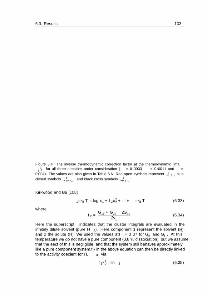
6.3. Results 103
Figure 6.4: The inverse thermodynamic correction factor at the thermodynamic limit,Γ−1ij,∞ for all three densities under consideration (ρ∗ = 0.0003, ρ∗ = 0.0011 and ρ∗ =
0.004). The values are also given in Table 6.6. Red open symbols represent Γ−1HH,∞, blue
closed symbols Γ−1H2H2,∞ and black cross symbols Γ−1
HH2,∞.
Kirkwood and Buff [108]
µ1/kBT = log x1 + f2x22 + ...+ µ◦/kBT (6.33)
where
f2 =G◦11 +G◦22 − 2G◦12
2v◦1(6.34)
Here the superscript ◦ indicates that the cluster integrals are evaluated in theinfinitely dilute solvent (pure H2). Here component 1 represent the solvent (H2)and 2 the solute (H). We used the values at T ∗ = 0.07 for G◦ii and G◦ij . At thistemperature we do not have a pure component (0.8 % dissociation), but we assumethat the effect of this is negligible, and that the system still behaves approximatelylike a pure component system. f2 in the above equation can then be directly linkedto the activity coefficient for H, γH, via
f2x22 = ln γ2 (6.35)
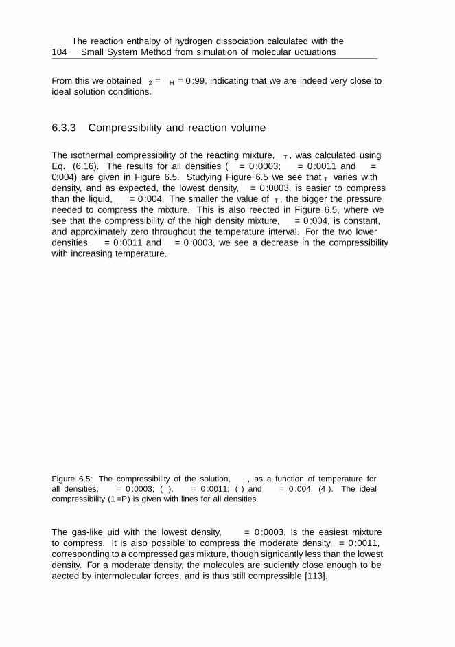
104The reaction enthalpy of hydrogen dissociation calculated with the
Small System Method from simulation of molecular fluctuations
From this we obtained γ2 = γH = 0.99, indicating that we are indeed very close toideal solution conditions.
6.3.3 Compressibility and reaction volume
The isothermal compressibility of the reacting mixture, κT , was calculated usingEq. (6.16). The results for all densities (ρ∗ = 0.0003; ρ∗ = 0.0011 and ρ∗ =0.004) are given in Figure 6.5. Studying Figure 6.5 we see that κT varies withdensity, and as expected, the lowest density, ρ∗ = 0.0003, is easier to compressthan the liquid, ρ∗ = 0.004. The smaller the value of κT , the bigger the pressureneeded to compress the mixture. This is also reflected in Figure 6.5, where wesee that the compressibility of the high density mixture, ρ∗ = 0.004, is constant,and approximately zero throughout the temperature interval. For the two lowerdensities, ρ∗ = 0.0011 and ρ∗ = 0.0003, we see a decrease in the compressibilitywith increasing temperature.
0
2e-09
4e-09
6e-09
8e-09
1e-08
1.2e-08
0.05 0.1 0.15 0.2 0.25 0.3 0.35 0.4
κ T [
Pa-1
]
T*
ρ*=0.0003ρ*=0.0011ρ*=0.004
ideal ρ*=0.0003ideal ρ*=0.0011ideal ρ*=0.004
Figure 6.5: The compressibility of the solution, κT , as a function of temperature forall densities; ρ∗ = 0.0003; (�), ρ∗ = 0.0011; (◦) and ρ∗ = 0.004; (4). The idealcompressibility (1/P ) is given with lines for all densities.
The gas-like fluid with the lowest density, ρ∗ = 0.0003, is the easiest mixtureto compress. It is also possible to compress the moderate density, ρ∗ = 0.0011,corresponding to a compressed gas mixture, though significantly less than the lowestdensity. For a moderate density, the molecules are sufficiently close enough to beaffected by intermolecular forces, and is thus still compressible [113].
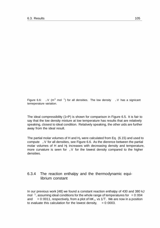
6.3. Results 105
5e-05
0.0001
0.00015
0.0002
0.00025
0.0003
0.00035
0.05 0.1 0.15 0.2 0.25 0.3 0.35 0.4
∆ r V
[m
3 mol
-1]
T*
ρ*=0.0003ρ*=0.0011ρ*=0.004
Figure 6.6: ∆rV (m3 mol−1) for all densities. The low density ∆rV has a significanttemeperature variation.
The ideal compressibility (1/P ) is shown for comparison in Figure 6.5. It is fair tosay that the low density mixture at low temperature has results that are relativelyspeaking, closest to ideal condition. Relatively speaking, the other fluids are furtheraway from the ideal result.
The partial molar volumes of H and H2 were calculated from Eq. (6.15) and used tocompute ∆rV for all densities, see Figure 6.6. As the difference between the partialmolar volumes of H and H2 increases with decreasing density and temperature,more curvature is seen for ∆rV for the lowest density compared to the higherdensities.
6.3.4 The reaction enthalpy and the thermodynamic equi-librium constant
In our previous work [48] we found a constant reaction enthalpy of 430 and 380 kJmol−1, assuming ideal conditions for the whole range of temperatures for ρ∗ = 0.004and ρ∗ = 0.0011, respectively, from a plot of lnKx vs 1/T . We are now in a positionto evaluate this calculation for the lowest density, ρ∗ = 0.0003.
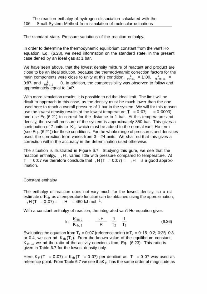
106The reaction enthalpy of hydrogen dissociation calculated with the
Small System Method from simulation of molecular fluctuations
The standard state. Pressure variations of the reaction enthalpy.
In order to determine the thermodynamic equilibrium constant from the van’t Hoffequation, Eq. (6.23), we need information on the standard state, in the presentcase defined by an ideal gas at 1 bar.
We have seen above, that the lowest density mixture of reactant and product areclose to be an ideal solution, because the thermodynamic correction factors for themain components were close to unity at this condition, Γ−1
HH,∞ = 1.00, Γ−1H2H2,∞ =
0.87, and Γ−1HH2,∞ ≈ 0. In addition, the compressibility was observed to follow and
approximately equal to 1/P .
With more simulation results, it is possible to find the ideal limit. The limit will bedifficult to approach in this case, as the density must be much lower than the oneused here to reach a overall pressure of 1 bar in the system. We will for this reasonuse the lowest density results at the lowest temperature, (T ∗ = 0.07, ρ∗ = 0.0003),and use Eq.(6.21) to correct for the distance to 1 bar. At this temperature anddensity, the overall pressure of the system is approximately 850 bar. This gives acontribution of 7 units to Kth which must be added to the normal van’t Hoff term(see Eq. (6.21)) for these conditions. For the whole range of pressures and densitiesused, the correction term varies from 3 - 24 units. We shall find that this gives acorrection within the accuracy in the determination used otherwise.
The situation is illustrated in Figure 6.7. Studying this figure, we see that thereaction enthalpy, ∆rH, varies little with pressure compared to temperature. AtT ∗ = 0.07 we therefore conclude that ∆rH(T ∗ = 0.07) = ∆rH
is a good approx-imation.
Constant enthalpy
The enthalpy of reaction does not vary much for the lowest density, so a firstestimate of Kth as a temperature function can be obtained using the approximation,∆rH(T ∗ = 0.07) = ∆rH
= 460 kJ mol−1.
With a constant enthalpy of reaction, the integrated van’t Hoff equation gives
ln
(Kth,2
Kth,1
)= −∆rH
R
(1
T2− 1
T1
)(6.36)
Evaluating the equation from T1 = 0.07 (reference point) to T2 = 0.15, 0.2, 0.25, 0.3or 0.4, we can find Kth(T2). From the known value of the equilibrium constant,Kth,1, we find the ratio of the activity coefficients from Eq. (6.23). This ratio isgiven in Table 6.7 for the lowest density only.
Here, KP (T ∗ = 0.07) = Kth(T ∗ = 0.07) per definition as T ∗ = 0.07 was used asreference point. From Table 6.7 we see that Kth has the same order of magnitude as

6.3. Results 107
Figure 6.7: Reaction enthalpy, ∆rH as a function of the reduced temperature (T ∗) andpressure (P ∗) and the fraction of H2 in the system (xH2), for all densities.
Table 6.7: Kth and KP and γ2H/γH2 as a function of the temperature, assuming that
∆rH = 460 kJ/mol is constant, at ρ∗ = 0.0003.
T ∗ Kth KP γ2H/γH2
0.15 722 628 1.20.2 4256 4116 1.00.25 12335 9344 1.30.3 25075 24356 1.00.4 60867 45778 1.3

108The reaction enthalpy of hydrogen dissociation calculated with the
Small System Method from simulation of molecular fluctuations
KP and that the fraction of the activity coefficients varies from 1.0–1.3, indicatingthat we have attractive forces acting between H and H2 (assuming γH = 0.99(Eq. (6.35)) is constant over the temperature interval and γH2
< 1). This is soaccording to standard mixture theory when we compare with an ideal mixtureof pure components. As one would expect H and H2 to repel each other, this isunexpected.
Enthalpy varies with temperature
The temperature dependence on the enthalpy was next included in the van’t Hoffequation.
The variation in ∆rH as obtained from as a function of temperature, is given inFigure 6.8 in reduced units for all densities. The line in the bottom of the plotcorresponds to the value found for the enthalpy by assuming the ideal conditionused before (plot of lnKx vs 1/T ) [48].
The reaction enthalpy (in J mol−1) was now fitted to a quadratic function of thetemperature, giving
∆rH(ρ∗ = 0.0003) = 0.0003T 2 − 8.9T + 4.9 · 105 (6.37)
∆rH(ρ∗ = 0.0011) = 0.0006T 2 − 19.5T + 5.5 · 105 (6.38)
∆rH(ρ∗ = 0.004) = 0.0007T 2 − 31.3T + 6.5 · 105 (6.39)
We rewrite the van’t Hoff equation, using the identity d(1/T ) = −(1/T 2)dT , and∆rH = aT 2 + bT + c and obtain after integration
ln
(Kth,2
Kth,1
)=
1
R
[aT + b lnT − c
T
]∣∣∣∣2
1
(6.40)
The thermodynamic equilibrium constant and the ratio of the activity coefficients,calculated from this equation and Eq.6.23 are shown Table 6.8 for the lowest density.When we include the temperature dependence in ∆rH we see from Table 6.8 that
Table 6.8: Kth and γ2H/γH2 as a function of the temperature at ρ∗ = 0.0003 assuming the
enthalpy of the reaction is described by a polynomial fit.
T ∗ Kth KP γ2H/γH2
0.15 604 628 1.00.2 3208 4126 0.80.25 8606 9344 0.90.3 16564 24356 0.70.4 37932 45778 0.8
we get Kth in the same order of magnitude as KP and Kth from Table 6.7 (wherewe used a constant ∆rH). The ratio of the activity coefficients are not constant
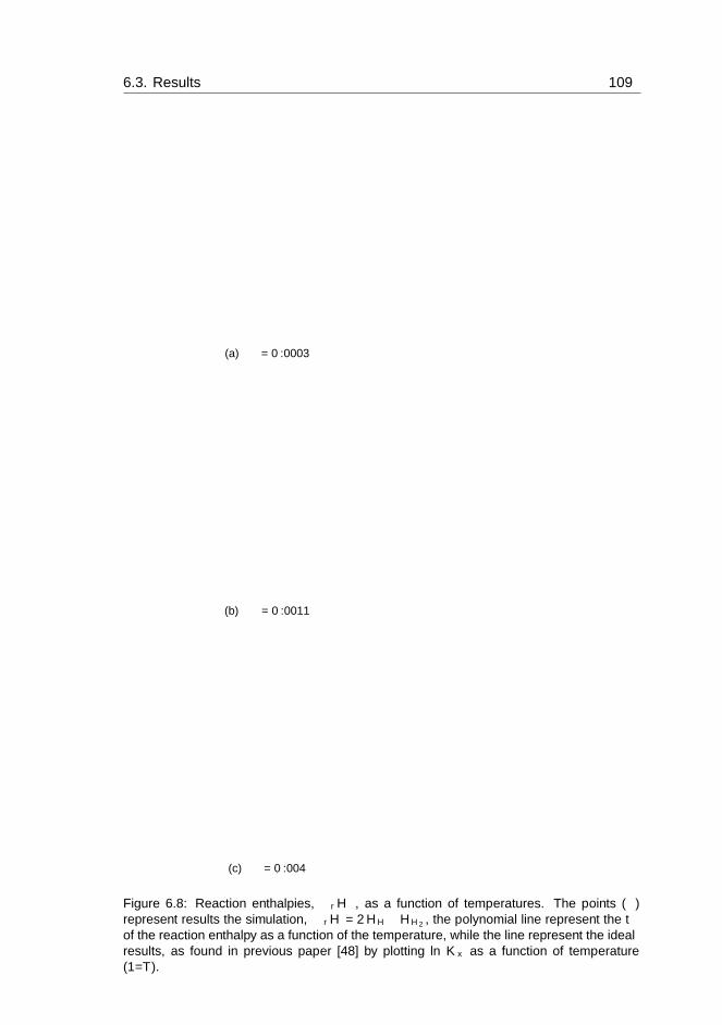
6.3. Results 109
0.8
0.85
0.9
0.95
1
1.05
1.1
0.05 0.1 0.15 0.2 0.25 0.3 0.35 0.4
∆ r H
*
T*
∆r H*
ideal approx
(a) ρ∗ = 0.0003
0.85
0.9
0.95
1
1.05
1.1
1.15
0.05 0.1 0.15 0.2 0.25 0.3 0.35 0.4
∆ r H
*
T*
∆r H*
ideal approx
(b) ρ∗ = 0.0011
0.7
0.8
0.9
1
1.1
1.2
1.3
1.4
0.05 0.1 0.15 0.2 0.25 0.3 0.35 0.4
∆ r H
*
T*
∆r H*
ideal approx
(c) ρ∗ = 0.004
Figure 6.8: Reaction enthalpies, ∆rH∗, as a function of temperatures. The points (�)
represent results the simulation, ∆rH = 2HH−HH2 , the polynomial line represent the fitof the reaction enthalpy as a function of the temperature, while the line represent the idealresults, as found in previous paper [48] by plotting lnKx as a function of temperature(1/T ).
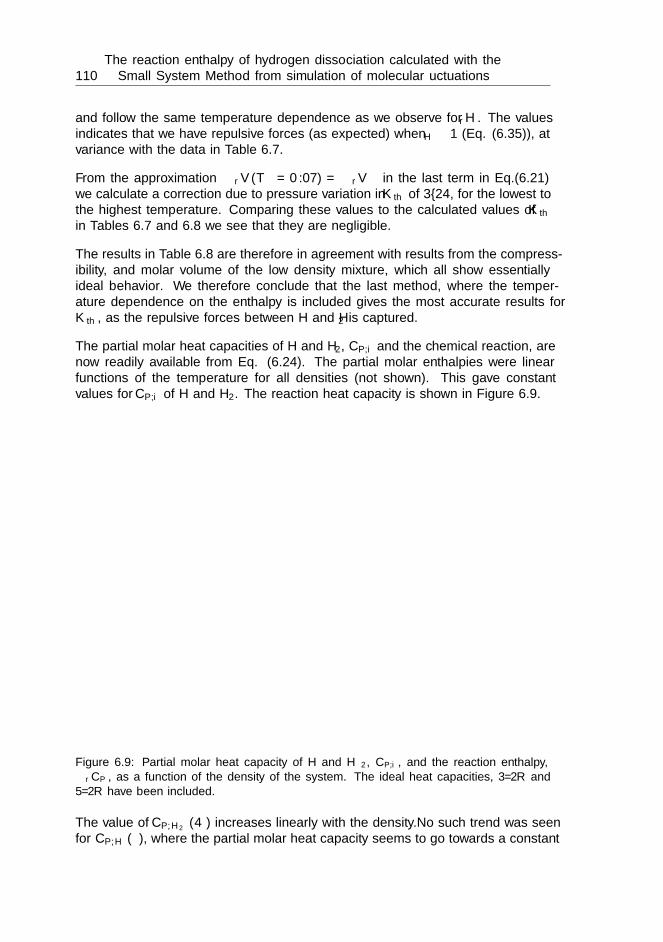
110The reaction enthalpy of hydrogen dissociation calculated with the
Small System Method from simulation of molecular fluctuations
and follow the same temperature dependence as we observe for ∆rH. The valuesindicates that we have repulsive forces (as expected) when γH ≈ 1 (Eq. (6.35)), atvariance with the data in Table 6.7.
From the approximation ∆rV (T ∗ = 0.07) = ∆rV in the last term in Eq.(6.21)
we calculate a correction due to pressure variation in Kth of 3–24, for the lowest tothe highest temperature. Comparing these values to the calculated values of Kth
in Tables 6.7 and 6.8 we see that they are negligible.
The results in Table 6.8 are therefore in agreement with results from the compress-ibility, and molar volume of the low density mixture, which all show essentiallyideal behavior. We therefore conclude that the last method, where the temper-ature dependence on the enthalpy is included gives the most accurate results forKth, as the repulsive forces between H and H2 is captured.
The partial molar heat capacities of H and H2, CP,i and the chemical reaction, arenow readily available from Eq. (6.24). The partial molar enthalpies were linearfunctions of the temperature for all densities (not shown). This gave constantvalues for CP,i of H and H2. The reaction heat capacity is shown in Figure 6.9.
-20-10
0 10 20 30 40 50 60 70 80 90
0.0005 0.0015 0.0025 0.0035
Cp
[J/m
ol K
]
ρ*
∆r Cp
3/2R
H
H2
5/2R
Figure 6.9: Partial molar heat capacity of H and H2, CP,i, and the reaction enthalpy,∆rCP , as a function of the density of the system. The ideal heat capacities, 3/2R and5/2R have been included.
The value of CP,H2 (4) increases linearly with the density.No such trend was seenfor CP,H (◦), where the partial molar heat capacity seems to go towards a constant
6.4. Conclusions 111
value. This is reasonable, as the atom has only kinetic degrees of freedom and atheoretical ideal heat capacity of 5
2R. For the molecule, there are at least two more(rotational) degrees of freedom, and the possibility for activation of a vibrationaldegree of freedom.
6.3.5 The method
We have seen above that the Small System Method can be used to give accuratedata for chemical reactions. Using the hydrogen dissociation reaction as exam-ple, we have calculated all relevant thermodynamic data for the reaction from onesimulation at different temperatures and densities. The computations may seemcumbersome, by having to change between ensembles, but the transformation pro-cedure is well established [25,109]. The bonus is that information can be obtainedabout non-ideal behavior in mixtures and chemical reactions. This information isotherwise not easily accessible. This is promising for the future, as new force fieldsbecome available for calculation of chemical reactions using classical potentials,such as ReaxFF [38], REBO [39] and AIREBO [40].
The results elucidate that the normal assumption, to take the reaction enthalpyconstant in the integration of van’t Hofff’s equation, can be much improved, seeFigure 6.8. We see that the biggest error is observed for the low density, where theideal value, assuming Kth = Kx, is far below the calculated value of the reactionenthalpy using the Small System Method. The calculated reaction enthalpy isfor all densities in the same order of magnitude (350–460 kJ mol−1) for ρ∗ =0.0003−−ρ∗ = 0.004 as the enthalpy of reaction at standard state conditions (436kJ mol−1) and the previous results obtained by us [48] 430 and 380 kJ mol−1 forρ∗ = 0.004 and ρ∗ = 0.0011, respectively.
6.4 Conclusions
We have applied a new calculation method, the Small System Method, to sampledata on particle and energy fluctuations, and find partial molar enthalpies andreaction enthalpies for the dissociation of hydrogen molecules to atoms. Data forthe thermodynamic correction factor, compressibility, heat capacity and partialmolar volumes were also obtained, all from the same set of simulations. The ther-modynamic equilibrium constant was determined as a function of pressure andtemperature for the lowest density studied, ρ∗ = 0.0003. It was observed that thevariation of the enthalpy with temperature was important to find the correct valueof Kth.
We have earlier seen that the hydrogen dissociation reaction was far from ideal, asjudged by contributions to i.e. the total pressure from the two-and three particleinteraction potential, in spite of showing an apparently ideal behavior in terms of
112The reaction enthalpy of hydrogen dissociation calculated with the
Small System Method from simulation of molecular fluctuations
pressure. In the present paper we see that even though we find the compressibilityand the molar volume of the low density to give ideal behavior, non-ideality isobserved in the heat capacity and the ratio of activity coefficients. From this weconclude that the method can provide information on the non-ideality of a system,which is information that is presently difficult to obtain, in a computationallyeffective way.
Acknowledgement
RS is grateful to Storforsk Project Transport nr. 167336 from NFR and the De-partment of Chemistry, NTNU, for financial support.
Chapter 7
Diffusion of heat and mass ina chemical reacting mixture
Ragnhild Skorpa1, Thijs J. H. Vlugt2, Dick Bedeaux1 andSigne Kjelstrup1
1. Department of Chemistry,Norwegian University of Science and Technology,
NO-7491 Trondheim, Norway
2. Process & Energy Laboratory, Delft University of Technology,Leeghwaterstraat 39, 2628CB Delft, The Netherlands
This chapter is included as a manuscript draft

Is not included due to copyright

Chapter 8
Conclusions
The aim of this thesis project has been to model chemical reactions under bothequilibrium and non-equilibrium conditions using classical molecular dynamics sim-ulations. From this the aim was to improve and extend the existing methodologyfor describing chemical reactions, and gain knowledge about the nature of disso-ciative reactions. The dissociation of hydrogen H2 2H was used as a modelsystem. This reaction is inevitable in producing hydrogen for fuel cells etc. us-ing a palladium membrane reactor. Knowledge about the process is thus of greatimportance. This was illustrated by showing how a temperature gradient over amembrane could be used to enhance and control the flux of hydrogen through themembrane.
A temperature range where a significant degree of dissociation was present wasdetermined using equilibrium molecular dynamics simulations. The Small SystemMethod was extended to find partial molar enthalpies for both a non-reactive anda reactive system. From this the reaction enthalpy of the hydrogen dissociationreaction as a function of temperature, pressure and composition of the reactingmixture was found. Three different densities was studied, a gas (0.0052 g/cm3), acompressed gas (0.0191 g/cm3) and a liquid (0.0695 g/cm3). Knowing the reactionenthalpy, it was possible to determine how far the system was from ideal conditions,and to find the thermodynamic equilibrium constant for a low density gas.
Knowing the equilibrium properties of the reaction, a temperature gradient wasapplied to the system. Based on analytical expressions for the mass flux andinverse temperature profiles the phenomenological coefficients and the transportproperties of the system was determined, even though the reaction was observedto be far from chemical equilibrium, close to the thermostatted regions.
Thus, a model which can facilitate further studies of the impact of chemical reac-tions on transport systems has been made. The Small System Method makes itpossible to determine e.g., reaction enthalpies for a linear dependent system, from
135

136 Conclusions
one simulation alone. The use of non-equilibrium thermodynamics makes it pos-sible to describe and quantify the coupled heat and mass transport, which can inturn be used to e.g., enhance the hydrogen flux through a palladium membrane.
Chapter 9
Suggestions for further work
In this study classical molecular dynamics simulations have been used to studythe dissociative hydrogen reaction under both equilibrium and non-equilibriumconditions. The newly developed extension to the Small System Method also madeit possible to determine the reaction enthalpy as a function of temperature, pressureand composition. Based on the obtained results, some possibilities for furtherstudies has been included below.
As the Small System Method has been incorporated into the familiar LAMMPSprogram, it is now easily accessible, for a variety of reactive and non-reactive force-fields. This means that partial molar enthalpies and reaction enthalpies can becalculated for a variety of systems. The method also gives access to the thermody-namic correction factor from which the chemical potential and activity coefficientcan be found for a binary mixture. The thermodynamic correction factor canalso be used to find Fick diffusion coefficients. These quantities are of interest forchemists and the chemical industry.
An interesting and natural extension of this thesis project would be to includea surface, e.g., palladium and study the reaction on a surface. The dissociativereaction of hydrogen on a palladium surface is important in a membrane reactoras discussed in this thesis. The Small System Method has already been extendedto surfaces [59] and adding a temperature gradient would suite as a driving forcefor the chemical reaction. Non-equilibrium thermodynamics would also be a usefultool to study the temperature at the palladium surface.
In the last study, where non-equilibrium molecular dynamics was used to findtransport coefficients, the thermal conductivity and heat of transfer in the presenceof a chemical reaction was observed to be higher than expected. However, thesequantities for a reactive system are scarcely reported in literature, and more studiescould thus be beneficial to verify the observed results.
137


Bibliography
[1] F. H. Stillinger and T. A. Weber. Computer simulation of local order incondensed phases of silicon. Phys. Rev. B, 31:5262–5271, Apr 1985.
[2] F. H. Stillinger and T. A. Weber. Molecular dynamics study of chemicalreactivity in liquid sulfur. J. Phys. Chem., 91:4899–4907, 1987.
[3] F. H. Stillinger and T. A. Weber. Molecular dynamics simulation for chemi-cally reactive substances. Fluorine. J. Chem. Phys., 8:5123–5133, 1988.
[4] M. W. Finnis and J. E. Sinclair. A simple empirical n-body potential fortransition metals. Philosophical Magazine A, 50(1):45–55, 1984.
[5] G. C. Abell. Empirical chemical pseudopotential theory of molecular andmetallic bonding. Phys. Rev. B, 31:6184–6196, May 1985.
[6] L. Schlapbach and Zuttel. Hydrogen-storage materials for mobile applica-tions. Nature, 414:353–358, 2001.
[7] M. Momirlan and Veziroglu T. N. The properties of hydrogen as fuel tomor-row in sustainable energy system for a cleaner planet. Int. J. of HydrogenEnergy, 30(7):795 – 802, 2005.
[8] A. F. Holleman, E. Wiberg, and N. Wiberg. Inorganic Chemistry. Academicpress, California, USA, 2001.
[9] D. Mendes, A. Mendes, L. M. Madeira, A. Iulianelli, J. M. Sousa, andA. Basile. The water-gas shift reaction: from conventional catalytic sys-tems to Pd-based membrane reactors — a review. Asia-Pac. J. Chem. Eng.,5:111–137, 2010.
[10] A. Basile. Hydrogen production using Pd-based membrane reactors for fuelcells. Topics in Catalysis, 51:107–122, 2008.
[11] S. Yun and S. T. Oyama. Correlations in palladium membranes for hydrogenseparation: A review. J. Mem. Sci., 375:28–45, 2011.
139
140 Bibliography
[12] S. Kjelstrup and D. Bedeaux. Non-equilibrium thermodynamics of heteroge-neous systems. World Scientific, 2008.
[13] B. Hafskjold and T. Ikeshoji. Partial specific quantities computed by nonequi-librium molecular dynamics. Fluid Phase Equilibria, 104:173–184, 1995.
[14] S. I. Sandler. Chemical, Biochemical, and Engineering Thermodynamics.Wiley, 2006.
[15] P. Atkins and J. De Paula. Atkins’ Physical Chemisty. Freeman, 8th edition,2006.
[16] F. Daniels, J. W. Williams, P. Bender, R. A. Alberty, C. D. Cornwell, andJ. E. Harriman. Experimental Physical Chemistry. McGraw-Hill, 7th edition,1970.
[17] S. Sunner and M. Mansson. Experimental Chemical Thermodynamics. Vol-ume 1. Combustion Calorimetry. Pergamon Press, 1979.
[18] F. A. Bettelheim. Experimental Physical Chemistry. W. B. Saunders Com-pany, 1971.
[19] P. Sindzingre, G. Ciccotti, C. Massobrio, and D. Frenkel. Partial enthalpiesand related quantities in mixtures from computer simulation. Chem. Phys.Lett., 136:35–41, 1987.
[20] D. Frenkel and B. Smit. Understanding Molecular Simulations. From Algo-rithms to Applications. Academic Press, 2. edition, 2002.
[21] P. Sindzingre, C. Massobrio, G. Ciccotti, and D. Frenkel. Calculation ofpartial enthalpies of an Argon-Krypton mixture by NPT molecular dynamics.Chem. Phys., 129:213–224, 1989.
[22] S. K. Schnell, T. J. H. Vlugt, J.-M. Simon, D. Bedeaux, and S. Kjelstrup.Thermodynamics of a small system in a µt reservoir. Chem. Phys. Lett.,504:199–201, 2011.
[23] S. K. Schnell, X. Liu, J.-M. Simon, A. Bardow, D. Bedeaux, T. J. H. Vlugt,and S. Kjelstrup. Calculating Thermodynamic Properties from Fluctuationsat Small Scales. J. Phys. Chem. B, 115:10911–10918, 2011.
[24] S. K. Schnell, T. J. H. Vlugt, J.-M. Simon, D. Bedeaux, and S. Kjelstrup.Thermodynamics of small systems embedded in a reservoir: a detailed analy-sus of finite size effects. Mol. Phys., 110:1069–1079, 2012.
[25] S. K. Schnell, R. Skorpa, D. Bedeaux, S. Kjelstrup, T. J. H. Vlugt, and J.-M.Simon. Partial Molar Enthalpies and Reaction Enthalpies From EquilibriumMolecular Dynamics Simulation. Submitted to JPC, 2014.

Bibliography 141
[26] J. Xu, S. Kjelstrup, D. Bedeaux, and J.-M. Simon. Transport properties of2FF2 in a temperature gradient as studied by molecular dynamics simula-tions. Phys. Chem. Chem. Phys., 9:969–981, 2007.
[27] D. C. Rapaport. The Art of Molecular Dynamics Simulations. CambridgeUniversity Press, 2 edition, 2005.
[28] M. P. Allen and D. J. Tildesley. Computer Simulation of Liquids. OxfordUniversity Press, New York, 1987.
[29] D. Kohen, J. C. Tully, and F. H. Stillinger. Modeling the interaction ofhydrogen with silicon surfaces. Surface Science, 397:225–236, 1998.
[30] J. Xu, S. Kjelstrup, D. Bedeaux, A. Rœsjorde, and L. Rekvig. Verificationof onsager’s reciprocal relations for evaporation and condensation using non-equilibrium molecular dynamics. J. Colloid Interf. Sci., 299:452–463, 2006.
[31] J. Xu, S. Kjelstrup, and D. Bedeaux. Molecular dynamics simulations of achemical reaction; conditions for local equilibrium in a temperature gradient.Phys. Chem. Chem. Phys., 8:2017–2027, 2006.
[32] J. Xu, S. Kjelstrup, D. Bedeaux, and J.-M. Simon. The heat of transfer ina chemical reaction at equilibrium. J. Non-Equilib. Thermodyn., 32:341–349,2007.
[33] B. M. Axilrod and E. Teller. Interaction of the van der Waals type betweenthree atoms. J. Chem. Phys., 11:299–300, 1943.
[34] R. J. Sadus. Exact calculation of the effect of three-body Axilrod-Teller inter-actions on vapour-liquid phase coexistence. Fluid Phase Equilibria, 144:351–359, 1998.
[35] R. J. Sadus. The effect of three-body interactions on the liquid-liquid phasecoexistence of binary fluid mixtures. Fluid Phase Equilibria, 150:63–72, 1998.
[36] J. Tersoff. New empirical approach for the structure and energy of covalentsystems. Phys. Rev. B, 37:6991–7000, Apr 1988.
[37] D. W Brenner. Empirical potential for hydrocarbons for use in simulating thechemical vapor deposition of diamond films. Phys. Rev. B, 42(15):9458–9471,1990.
[38] A. C. T. van Duin, S. Dasgupta, F. Lorant, and W. A. Goddard III. ReaxFF:A reactive force field for hydrocarbons. J. Phys. Chem. A, 105:9396–9409,2001.
[39] D. W. Brenner, O. A. Shenderova, J. A. Harrison, S. J. Stuart, B. Ni, andS. B. Sinnott. A second-generation reactive empirical bond order (rebo)potential energy expression for hydrocarbons. J. Phys.: Condens. Matter,14:783–802, February 2002.
142 Bibliography
[40] S. J. Stuart, A. B. Tutein, and J. A. Harrison. A reactive potential forhydrocarbons with intermolecular interactions. J. Phys. Chem., 112:6472–6486, April 2000.
[41] Kimberly Chenoweth, Adri C.T. van Duin, Petter Persson, Mu-Jeng Cheng,Jonas Oxgaard, and William A. Goddard, III. Development and applica-tion of a reaxff reactive force field for oxidative dehydrogenation on vana-dium oxide catalysts. J. Phys. Chem. C, 112(37):14645–14654, 2008. PMID:18652441.
[42] III Goddard, WilliamA., Adri Duin, Kimberly Chenoweth, Mu-Jeng Cheng,Sanja Pudar, Jonas Oxgaard, Boris Merinov, YunHee Jang, and Petter Pers-son. Development of the reaxff reactive force field for mechanistic studiesof catalytic selective oxidation processes on bimoo x. Topics in Catalysis,38(1-3):93–103, 2006.
[43] Kevin D. Nielson, Adri C. T. van Duin, Jonas Oxgaard, Wei-Qiao Deng,and William A. Goddard. Development of the reaxff reactive force field fordescribing transition metal catalyzed reactions, with application to the initialstages of the catalytic formation of carbon nanotubes. J. Phys. Chem. A,109(3):493–499, 2005.
[44] Jeffery Ludwig, Dionisios G. Vlachos, Adri C. T. van Duin, and William A.Goddard. Dynamics of the dissociation of hydrogen on stepped platinumsurfaces using the reaxff reactive force field. J. Phys. Chem. B, 110(9):4274–4282, 2006.
[45] F. H. Stillinger and T. A. Weber. Hidden structure in liquids. Phys. Rev. A,25:978–989, Feb 1982.
[46] D. L. Diedrich and J. B. Anderson. Exact quantum Monte Carlo calculationsof the potential energy surface for the reaction H +H2 → H2 + H. J. Chem.Phys., 100:8089–8095, 1994.
[47] D. L. Diedrich and J. B. Anderson. An accurate quantum Monte Carlocalculation of the barrier height for the reaction H +H2 = H2 + H. Science,258:786–788, 1992.
[48] R. Skorpa, J.-M. Simon, D. Bedeaux, and K. Kjelstrup. Equilibrium prop-erties of the reaction H2 2H. Phys. Chem. Chem. Phys., 6:1227–1237,2014.
[49] P. Siegbahn and B. Liu. An accurate three-dimensional potential energysurface for H3. J. Chem. Phys., 68:2457–2465, 1978.
[50] T. L. Hill. Thermodynamics of Small Systems, Part 1 and 2. Benjamin, NewYork, 1963.

Bibliography 143
[51] T. L. Hill and R. V. Chamberlin. Extension of the thermodynamics of smallsystems to open metastable states: An example. Proc. Natl. Acad. Sci.,95:12779–12782, 1998.
[52] T. L. Hill. Perspective: Nanothermodynamics. Nano Letters, 1:111–112,2001.
[53] T. L. Hill. A Different Approach to Nanothermodynamics. Nano Letters,1:273–275, 2001.
[54] X. Liu, S. K. Schnell, J.-M. Simon, D. Bedeaux, S. Kjelstrup, A. Bardow, andT. J. H. Vlugt. Fick Diffusion Coefficients of Liquid Mixtures Directly Ob-tained From Equilibrium Molecular Dynamics. J. Phys. Chem. B, 115:12921–12929, 2011.
[55] X. Liu, A. Martın-Calvo, E. McGarrity, S. K. Schnell, S. Calero, J.-M. Simon,D. Bedeaux, S. Kjelstrup, A. Bardow, and T. J. H. Vlugt. Fick Diffusion Co-efficients in Ternary Liquid Systems from Equilibrium Molecular DynamicsSimulations. Ind. Eng. Chem. Res., 51:10247–10258, 2012.
[56] S. K. Schnell, P. Englebienne, J.-M. Simon, P. Kruger, S. P. Balaji, S. Kjel-strup, D. Bedeaux, A. Bardow, and T. J. H Vlugt. How to apply theKirkwood-Buff theory to individual species in salt solutions. Chem. Phys.Lett., 582:154–157, 2013.
[57] J. Collell and G. Galliero. Determination of the thermodynamic correctionfactor of fluids confined in nano-metric slit pores from molecular simulation.J. Chem. Phys., 140(19):–, 2014.
[58] M. M. Reif, M. Winger, and C. Oostenbrink. Testing of the GROMOS Force-Field Parameter Set 54A8: Structural Properties of Electrolyte Solutions,Lipid Bilayers, and Proteins. J. Chem. Theory Comput., 9:1247–1264, 2013.
[59] T. T. Trinh, D. Bedeaux, J.-M. Simon, and S. Kjelstrup. Thermodynamiccharacterization of two layers of CO2 on a graphite surface. Chem. Phys.Lett., 612:214–218, 2014.
[60] S. Kjelstrup, D. Bedeaux, E. Johannesen, and J. Gross. Non-EquilibriumThermodynamics for Engineers. World Scientific, 2010.
[61] S. R. Groot and P. Mazur. Non-equilibrium thermodynamics. Dover Publi-cations, Inc., New York, 1984.
[62] L. Onsager. Reciprocal relations in irreversible processes. I. Phys. Rev.,37:404–426, 1931.
[63] L. Onsager. Reciprocal relations in irreversible processes. II. Phys. Rev.,38:2265–2279, 1931.

144 Bibliography
[64] R. Skorpa, M. Voldsund, M. Takla, S. K. Schnell, D. Bedeaux, and S. Kjel-strup. Assessing the coupled heat and mass transport of hydrogen throughpalladium membrane. J. Mem. Sci., 394–395:131–139, 2012.
[65] J. W. Gibbs. Scientific Papers: Thermodynamics. Dover Publications, Inc.,1961.
[66] E. E. McLeary, J. C. Jansen, and F. Kapteijn. Zeolite based films, membranesand membrane reactors: Progress and prospects. Micropor. Mesopor. Mater.,90:198–220, 2006.
[67] J. Coronas and J. Santamaria. State-of-the-art in zeolite membrane reactors.Topics in Catalysis, 29:29–44, 2004.
[68] T. P. Perng and J. K. Wu. A brief review note on mechanisms of hydrogenentry into metals. Materials Letters, 57:3437–3438, 2003.
[69] L. L. Jewell and B. H. Davis. Review of absorption and adsorption in thehydrogen-palladium system. Applied Catalysis A:General, 310:1–15, 2006.
[70] B. D. Morreale, M. V. Ciocco, R. M. Enick, B. I. Morsi, B. H. Howard,A. V. Cugini, and K. S. Rothenberger. The permeability of hydrogen in bulkpalladium at elevated temperatures and pressures. J. Mem. Sci., 212:87–97,2003.
[71] S. K. Gade, P. M. Thoen, and D. J. Way. Unsupported palladium alloyfoil membranes fabricated by electroless plating. J. Mem. Sci., 316:112–118,2008.
[72] T. L. Ward and T. Dao. Model of hydrogen permeation behavior in palladiummembranes. J. Mem. Sci., 153:211–231, 1999.
[73] I. J. Iwuchukwu and A. Sheth. Mathematical modeling of high temperatureand high-pressure dense membrane separation of hydrogen from gasification.Chemical Engineering and Processing, 47:1292–1304, 2008.
[74] A. Caravella, G. Barbieri, and E. Drioli. Modelling and simulation of hy-drogen permeation through supported Pd-alloy membranes with multicom-ponent approach. Chem. Eng. Sci., 63:2149–2160, 2008.
[75] M. Coroneo, G. Montante, J. Catalano, and A. Paglianti. Modelling theeffect of operating conditions on hydrodynamics and mass transfer in a Pd-Ag membrane module for H2 purification. J. Mem. Sci., 343:34–41, 2009.
[76] A. Bhargav and G. S. Jackson. Thermokinetic modeling and parameter esti-mation for hydrogen permeation through Pd0.77Ag0.23 membranes. Interna-tional Journal of Hydrogen Energy, 34:5164–5173, 2009.
Bibliography 145
[77] J. Catalano, M. G. Baschetti, and G. C. Sarti. Hydrogen permeation inpalladium-based membranes in the presence of carbon monoxide. J. Mem.Sci., 362:221–233, 2010.
[78] E. Johannessen and K. Jordal. Study of a H2 separating membrane reactorfor methane steam reforming at conditions relevant for power processes withCO2 capture. Energy Conversion and Management, 46:1059–1071, 2005.
[79] Y.-M. Lin, S.-L. Liu, C.-H. Chuang, and Y.-T. Chu. Effect of incipientremoval of hydrogen through palladium membrane on the conversion ofmethane steam reforming. Experimantal and modeling. Catalysis Today,82:127–139, 2003.
[80] J. Ge, S. Kjelstrup, D. Bedeaux, and J.-M. Simon. Transfer coefficients forevaporation of a system with a Lennard-Jones long-range spline potential.Phys. Rev. E, 75:061604, 2007.
[81] C. Y. Ho, R. W. Powell, and P. E. Liley. Thermal conductivity of the ele-ments. J. Phys. Chem. Ref. Data., 1:279–421, 1972.
[82] R. E. Buxbaum and T. L. Marker. Hydrogen transport through non-porousmembranes of palladium- coated niobium, tantalum and vanadium. J. Mem.Sci., 85:29–38, 1993.
[83] J.-M. Simon, O.-E. Haas, and S. Kjelstrup. Adsorption and desorptionof H2 on graphite by molecular dynamics simulations. J. Phys. Chem. C,114:10212–10220, 2010.
[84] V. Labet, P. Gonzalez-Morelos, R. Hoffman, and N. W. Ashcroft. A freshlook at dense hydrogen under pressure.I. An introduction to the problem,amd an index probing equalization of H-H distances. J. Chem. Phys., 136,2012.
[85] C. E. Thomas. Fuel cell and battery electric vehicles compared. Int. J.Hydrogen Energy, 34:6005–6020, 2009.
[86] F. T. Wagner, B. Lakshmanan, and M. F Mathias. Electrochemistry and theFuture of the Automobile. J. Phys. Chem. Lett, 1:2204–2219, 2010.
[87] P. T. Cummings and G. Stell. Statistical mechanical models of chemicalreactions. Mol. Phys., 51:253–287, 1984.
[88] W. R. Magro, D. M. Ceperley, C. Pierleoni, and B. Bernu. Molecular disso-ciation in hot, dense hydrogen. Phys. Rev. Lett., 76:1240–1243, 1996.
[89] K. T. Delaney, C. Pierleoni, and D. M. Ceperley. Quantum Monte Carlosimulation of the high-pressure molecular-atomic crossover in fluid hydrogen.Phys. Rev. Lett., 97:235702, 2006.
146 Bibliography
[90] H. Balamane, T. Halicioglu, and W. A. Tiller. Comparative study of siliconempirical interatomic potentials. Phys. Rev. B, 46:2250–2279, 1992.
[91] A. I. Boothroyd, P. G. Martin, W. J. Keogh, and M. J. Peterson. An accurateanalytic H4 potential energy surface. J. Chem. Phys., 116:666–689, 2002.
[92] G. Ciccotti and J. P. Ryckaert. Molecular dynamics simulation of rigidmolecules. Computer Physics Reports, 4:345–392, 1986.
[93] T. Ikeshoji and B. Hafskjold. Non-equilibrium molecular dynamics calcula-tion of heat conduction in liquid and through liquid-gas interface. Mol. Phys.,81:251–261, 1994.
[94] W. C. Swope, H. C. Andersen, P. H. Berens, and K. R. Wilson Wilson. Acomputer simulation method for the calculation of equilibrium constants forthe formation of physical clusters of molecules: Application to small waterclusters. J. Chem. Phys., 76(1):637–649, 1982.
[95] B. Militzer, W. Margo, and D. Ceperley. Characterization of the state ofhydrogen at high temperature and desity. Contrib. Plasma. Phys., 39:151–154, 1999.
[96] D. Saumon and G. Chabrier. Fluid hydrogen at high density: Pressure dis-sociation. Phys. Rev. A, 44:5122–5141, 1991.
[97] B. Militzer and D. M. Ceperley. Path integral Monte Carlo simulation of thelow-density hydrogen plasma. Phys. Rev. E, 63:066404, 2001.
[98] R. A. Alberty. Thermodynamics of Biochemical Reactions. Wiley-Interscience, 2003.
[99] T. Engell and P. Reid. Physical Chemistry. Prentice Hall, 2012.
[100] B. E. Poling, J. M. Prausnitz, and J. P. O. O’Connell. The properties of gasesand liquids. McGraw-Hill, New York, 5th edition, 2004.
[101] J. D. Weeks, D. Chandler, and H. C. Andersen. Role of repulsive forcesin determining the equilibrium structure of simple liquids. J. Chem. Phys.,54:5237–5247, 1971.
[102] P. Kruger, S. K. Schnell, D. Bedeaux, S. Kjelstrup, T. J. H. Vlugt, and J.-M.Simon. Kirkwood-Buff integrals for finite volumes. J. Phys. Chem. Lett.,4:235–238, 2013.
[103] R. Taylor and H. A. Kooijman. Composition derivatives of activity coefficientmodels (for the estimation of thermodynamic factors in diffusion). Chem.Eng. Comm., 102:87–106, 1991.
[104] R. Krishna and J. A. Wesselingh. The Maxwell-Stefan approach to masstransfer. Chem. Eng. Sci., 52(6):861–911, 1997.
Bibliography 147
[105] H. Hadwiger. Vorlesungen uber Inhalt, Oberflache und Isoperimetrie.Springer, 1957.
[106] K. R. Mecke. Integral geometry in statistical physics. Int. J. Mod. Phys. B,12:861–899, 1998.
[107] E. M. Blokhuis. Existence of a bending rigidity for a hard-sphere liquidnear a curved hard wall: Validity of the hadwiger theorem. Phys. Rev. E,87(2):022401, February 2013.
[108] J. G. Kirkwood and F. P. Buff. The Statistical Mechanical Theory of Solu-tions. I. J. Chem. Phys., 19:774–777, 1951.
[109] A. Ben-Naim. A molecular theory of solutions. Oxford University Press,2006.
[110] C. H. Turner, J. K. Brennan, M. Lisal, W. R. Smith, J. K. Johnson, andK. E. Gubbins. Simulation of chemical reaction equilibria by the reactionensemble monte carlo method: A review. Mol. Sim., 34:119–146, 2008.
[111] T. J. H. Vlugt and B. Smit. On the efficient sampling of pathways in thetransition path ensemble. PhysChemComm, 2:1–7, 2001.
[112] P. Sindzingre, G. Massobrio, C. Ciccotti, and D. Frenkel. Calculation ofpartial enthalpies of an argon-krypton mixture by NPT molecular dynamics.Chemical Physics, 129:213–224, 1989.
[113] K. S. Shing and S.-T. Chung. Calculation of Infinite-Dilution Partial MolarProperties by Computer Simulation. AIChE J., 34:1973–1980, 1988.
[114] P. G. Debenedetti. Fluctuationbased computer calculation of partial molarproperties. I. Molecular dynamics simulation of constant volume fluctuations.J. Chem. Phys., 86:7126, 1987.
[115] P. G. Debenedetti. Fluctuationbased computer calculation of partial mo-lar properties. II. A numerically accuarate method for the determination ofpartial molar energies and enthalpies. J. Chem. Phys., 88:2681, 1988.
[116] P. G. Debenedetti. Fluctuation Simulations and the Calculation of Mechan-ical Partial Molar Properties. Mol. Sim., 2:33–53, 1989.
[117] D. Saumon and G. Chabrier. Fluid hydrogen at high density: The plasmaphase transition. Phys. Rev. Lett., 62:2397–2400, May 1989.
[118] K. Sawada and T. Fujimoto. Effective ionization and dissociation rate coef-ficients of molecular hydrogen in plasma. J. Appl. Phys., 78(5):2913–2924,1995.
[119] D. A. Reed and G. Ehrlich. Surface diffusion, atomic jump rates and ther-modynamics. Surface Science, 102(2-3):588–609, 1981.
148 Bibliography
[120] R. B. Bird, W. E. Stewart, and E. N. Lightfoot. Transport phenomena. JohnWiley & Sons, 1960.
[121] J. N. Butler and R. S. Brokaw. Thermal Conductivity of Gas Mixtures inChemical Equilibrium. J. Chem. Phys., 26:1636–1643, 1957.
[122] R. B. Bird, W. E. Stewart, and E. N. Lightfoot. Transport phenomena. JohnWiley & Sons, 2nd. edition, 2006.
[123] R. Taylor and R. Krishna. Multicomponent Mass Transfer. Wiley, New York,1993.
[124] R. Skorpa, J.-M. Simon, D. Bedeaux, and K. Kjelstrup. The reaction enthalpyof hydrogen dissociation calculated with the Small System Method from sim-ulation of molecular fluctuations. Phys. Chem. Chem. Phys., 16:19681–19693,2014.
[125] F. Muller-Plathe. A simple nonequilibrium molecular dynamics method forcalculating the thermal conductivity. J. Chem. Phys., 106(14):6082–6085,1997.
[126] F. J. Uribe, E. A. Mason, and J. Kestin. Thermal conductivity of ninepolyatomic gases at low density. J. Chem. Phys. Ref. Data, 19:1123–1136,1990.