NOAA Contributions to the Central California Ozone Study and

Ongoing Meteorological Monitoring

Jim Wilczak

Jian-Wen Bao, Sara Michelson, Ola Persson, Laura Bianco, Irina Djalalova, and David E. White

NOAA/Earth Systems Research Laboratory

29 November 2006

Topics covered in this presentation (1)

1. Overview of project

2. Model optimization1. ABL

2. LSM

3. Surface emissivity (version 3.6 vs. 3.7)

4. Surface roughness lengths

5. Buoy comparison

6. Clouds and radiation

7. Initial and boundary conditions

8. Resolution

Topics covered in this presentation (2)

1. X

2. x

3. Data Assimilation1. Analysis nudging

2. Observation nudging

3. Sub-synoptic events

4. Data denial experiments

4. Trajectory analysis1. Profiler trajectory tool

2. Model trajectories

Topics covered in this presentation (3)

1. X

2. X

3. X

4. X

5. Impact of FDDA on ozone profiles

6. WRF simulations

7. Profiler maintenance

8. Seasonal modeling1. 15 day time series of surface met

2. Seasonal diurnal profiler/model composites

1. Overview of project• Project goals:

– Develop accurate model-based meteorological fields to be used as input to chemistry models

– Understand meteorology associated with high ozone events

• Began May 2002• Funding

– FY2002 ($250k) NOAA earmark– FY2003 ($250k) NOAA earmark– FY2004 ($250k) CCOS– FY2005($250k) NOAA earmark– FY2006 ($375) NOAA earmark

36km grid 95x91

12km grid 91x91

4km grid 190x190

All have 50 layers, with 22 in lowest 1km and lowest model level at 12m

MM5 Model Configuration

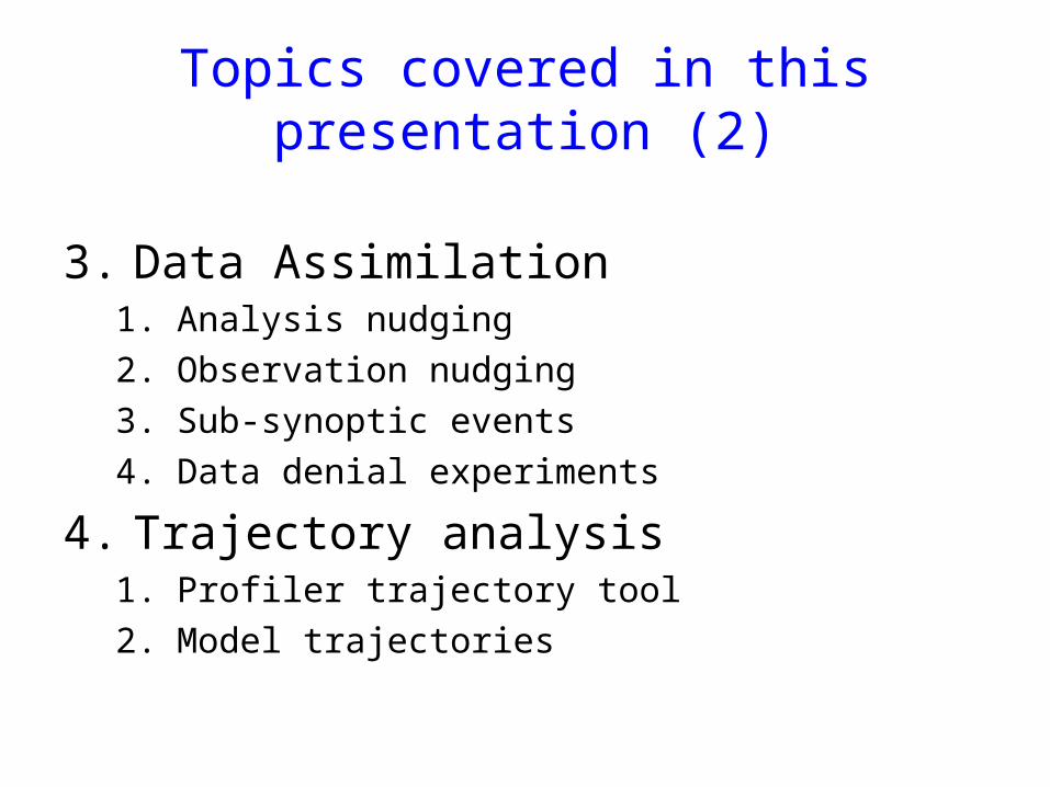
Observational Data SetsWind profiler sites

ABL schemes

Gayno-Seaman/5-layer soil MRF/5-layer soil

Eta/5-layer soil

Land Surface Modules

ObservationsEta/5-layer soilEta/NOAH LSM

Eta/NOAH LSM

Eta/5-layer soil (RED) and Eta/NOAH LSM (BLUE)Temperature errors averaged for all times at 25 profiler sites

0.9 C bias

Eta/5-layer soil (RED) and Eta/NOAH LSM (BLUE)wind errors averaged for all times at 25 profiler sites

0.6 m/s bias

ABL Depth Evaluation

Eta/NOAH LSM combination selected • Better phasing of diurnal variation of surface wind speed

• Comes closest to matching daytime max temperatures (other combinations have a larger cold bias) and Tdew

• Has much smaller temperature bias RMSE errors and wind speed bias above 100m than Eta/5-layer soil model

• However, has larger speed bias and RMSE in lowest 100m than Eta/5-layer

Philosophy: Select LSM with better temperature and moisture fields, explore other factors that may reduce surface winds, let FDDA correct for larger near-surface wind errors

Note: Later found that Eta/NOAH LSM wind errors with FDDA were smaller than Eta/5-layer soil model with FDDA

Surface emissivity

Corrected emissivity improves surface temperatures,but slightly degrades surface wind RMSE

Roughness length sensitivity

• MM5 specified z0 is 0.10-0.15 m in Central Valley

• Survey of literature of similar landscapes suggests a larger value of 0.30-0.75m.

• Ran numerical experiments increasing z0 by factors of 2, 5, and 10

Optimal z0 is about 5x larger,in agreement with literature values

Buoy comparison

0 20 40 60 80 100 120H o u r S ta rtin g 0 :0 0 U TC , Ju lia n D a y 2 1 2

0

2

4

6

8

10

12

Win

d S

peed [m

/s]

0 20 40 60 80 100 120H o u r

180

240

300

360

Win

d D

irect

ion [d

eg]

0 20 40 60 80 100 120H o u r

-2

0

2

4

6

8

U C

om

ponent [

m/s

]

0 20 40 60 80 100 120H o u r

-12

-8

-4

0

4

8

V C

om

ponent [

m/s

]

A rea B u oy 1

O b serv a tio n E T A M o d e l

O b serv a tio n an d M o d e l C o m p ariso n s

E m b : 0 .2 7E F m b : 0 .0 7

E T A -F D D A V 3 M o d e l

E a b : 1 .6 2E F a b : 1 .5 4

E sd : 1 .8 8E F sd : 1 .8 0

E m b : 6 .0 2E F m b : 5 .1 1

E a b : 2 0 .0 5E F a b : 2 0 .3 9

E sd : 3 8 .3 1E F sd : 3 9 .9 5

E m b : 0 .1 8E F m b : 0 .0 7

E a b : 1 .2 6E F a b :1 .2 2

E sd : 1 .4 3E F sd : 1 .3 9

E m b : -1 .1 0E F m b : -0 .8 7

E a b : 1 .7 6E F a b : 1 .7 0

E sd : 1 .7 6E F sd : 1 .7 8

Buoy comparison

z0 over oceanlooks OK

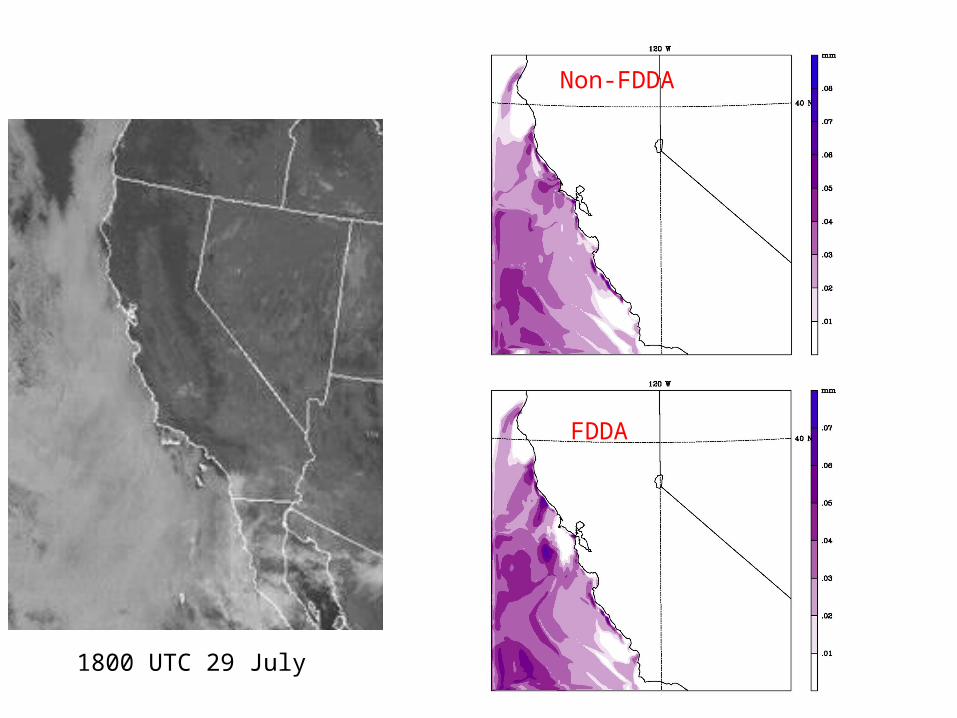
Clouds and radiation

• Compare satellite visible imagery with model integrated cloud liquid water

• Two distinct cloud types are present: low-level coastal stratus and upper-level clouds over land

Non-FDDA

FDDA

1800 UTC 29 July

Non-FDDA

FDDA

1800 UTC 30 July

1800 UTC 31 July

Non-FDDA FDDA

1800 UTC 1 Aug

Non-FDDA

FDDA

Non-FDDA FDDA

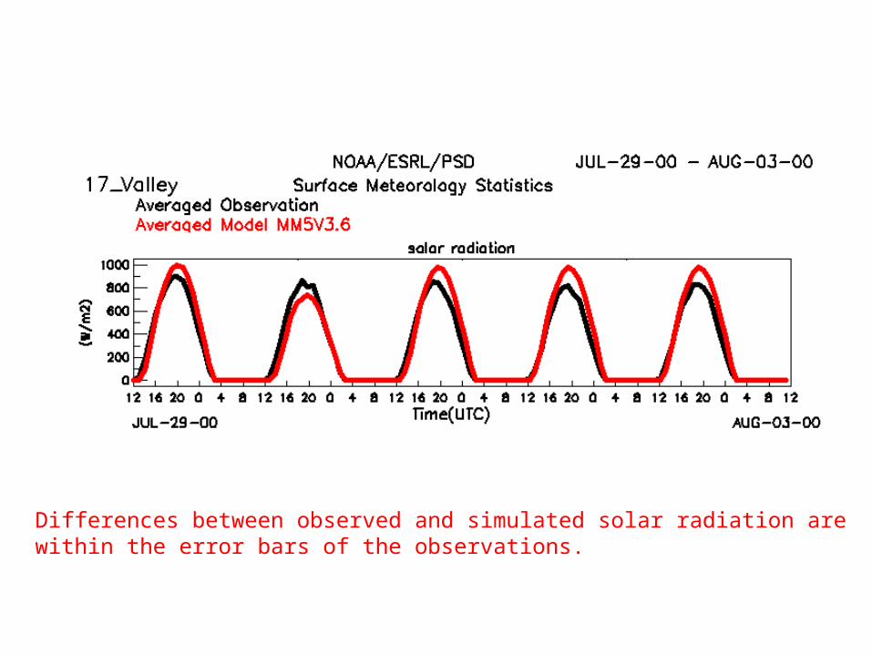
Differences between observed and simulated solar radiation arewithin the error bars of the observations.

Clouds and radiation summary• MM5 replicates patchy, intermittent coastal stratus

• MM5 also produces intermittent high-level clouds over land

• Timing and locations of clouds are not always correct, but cloud statistics appear ok

• FDDA can alter cloud fields, sometimes for the better, sometimes for worse

• MM5 solar radiation agrees with observations within the observational error

Initial and Boundary Conditions

• NCEP 40km Eta analysis (AWIPS)

• European Centre’s 0.5 deg (~50 km) analysis (ECMWF)

AWIPS ECMWF

850 mb temperatures (color shaded), geopotential heights (solid black contours) and winds at 1200 UTC 29 July 2000 from the AWIP and ECMWF analyseson the 36-km grid

AWIPS ECMWF

Initial and Boundary Conditions Summary

• Significant wind differences exist between the AWIPS and ECMWF simulations at any given time and height

• However, statistically one is not significantly better than the other

• ECMWF produces a larger surface cold bias

Horizontal grid resolution (1.33 vs. 4 km)

Average over all profiler sites except GLA

High resolution

• 1.33km resolution slightly improved the surface winds, reducing the high wind speed bias

• Higher resolution reduced nighttime cold bias, but also increased daytime cold bias by a smaller amount

• At some sites higher resolution led to more significant improvements

Four Dimensional Data Assimilation (FDDA)

• FDDA applies a correction term to the model equations at each time step that brings the model variables closer to the observed values

• The size of the correction term is proportional to the difference between the model variable and the observation

• If the model is already in reasonable agreement with the observations, the correction term is small, and the model remains in near dynamical balance

• Analysis (grid) nudging was applied on the 36 km grid using the time-interpolated 6-hourly AWIPS analyses. Winds, temperatures, and moisture were assimilated at heights above the model-diagnosed ABL height.

• Obs nudging was done for profiler and surface winds, using a 50 km e-folding radius of influence.

Observed winds Non-FDDA simulation

Arbuckle winds on 30 July 2000

Observed winds FDDA simulation

Arbuckle winds on 30 July 2000

Vector wind difference at Arbuckleon 30 July

Averages over 25 wind profiler sitesand all times

Averages over 25 wind profiler/RASS sitesand all times

• FDDA makes simulated and observed wind data almost indistinguishable from one another

• FDDA also significantly improves temperature bias and RMSE

• How far does influence of obs nudging extend away from profiler sites?

• Are their times when FDDA does not work well?

Data Denial ExperimentFDDA at all sites except CCO, SAC, SVS, AGO

Wind statistics averaged at 4 profiler sites (CCO, SAC, SVS, AGO)

Temperature statistics averaged at 4 profiler sites (CCO, SAC, SVS, AGO)

Effective radius of influence

RMSE for three simulations, MFDi, MFDiwh6, and MNFDRe(winds) ~ 50 kmRe(temp) ~ 260km

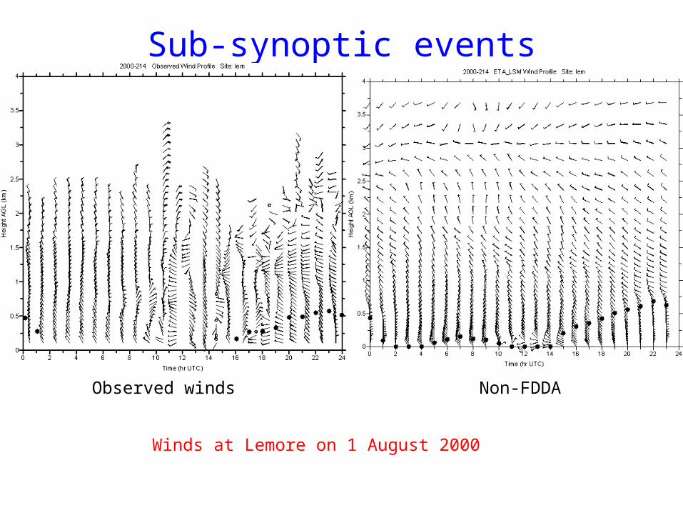
Sub-synoptic events

Observed winds Non-FDDA

Winds at Lemore on 1 August 2000

Observed winds FDDA winds

Winds at Lemore on 1 August 2000

24-h forward model trajectories for parcels released at SacramentoAt 00 UTC 31 July 2000. Red is for a release from the lowest model level, Blue 100m, and black 500m.

Non-FDDA FDDA

Trajectory Analysis

Trajectory Analysis

Wind profiler trajectory analysis tool

Trajectory Analysis

FDDA

Non-FDDA

Trajectory Analysis

• FDDA can make a significant difference in trajectory paths (trajectories are very sensitive to small changes in the winds)

• If attribution of specific ozone events is desired, FDDA is essential

• Purely observational and model trajectories can be calculated and compared

Effect of FDDA on vertical ozone profiles

Ozone statistics from 16 soundings taken at Granite Bay and Parlier.

Granite Bay: bias/no change; RMSE/improved; correlation/improvedParlier: bias/degraded; RMSE/no change; correlation/improve

WRF/MM5 Comparisons Southern Valley Averaged Temperature

10

15

20

25

30

35

40

0 24 48 72 96 120

Hours into Simulation from 00 UTC 30 July 2000

Tem

per

atu

re (

C)

Observations

MM5 etanoahlsm v3.7

WRF orig V2.1

2-m temperature averaged over the southern SJV

WRF is slightly warmer than MM5

Southern Valley Averaged Wind Speed

0

1

2

3

4

5

6

0 24 48 72 96 120

Hours into Simulation from 00 UTC 30 July 2000

Win

d S

pee

d (

m/s

)

Observations

MM5 etanoahlsm v3.7

WRF orig V2.1

10-m wind speed averaged over the southern SJV

WRF also has a high wind speed bias

WRF summary

• Relatively small differences were found between WRF and MM5

• NOAA’s WRF simulations were provided to BAAQD and run through CAMx, providing providing ozone simulations that were statistically equivalent to MM5

• WRF is ready for California AQ studies

Profiler Maintenance• NOAA maintained three profilers, at Chico, Chowchilla,

and Lost Hills• NOAA returned the Bay Area’s Livermore profiler to

service– Purchased a new system computer– Modified the radar controller card and coherent integrator card to

make them compatible with the revised PCI standard of the new computer system

– Replaced the DSP card with double the previous memory, which can allow for additional range gates

– Checked all antennas and switches– Replaced one RASS voice coil that was not working– Installed software that allows NOAA engineers to remotely

monitor the health of the profiler system, and to remotely upload modifications to the profiler operating system

– Initiated the real-time display of the Livermore data on NOAA’s profiler web site.

Seasonal Modeling

• QC’d 25x122=3050 profiler days of winds and RASS

• Provided 3050 days of ABL depths

• Ran 122 days of MM5 simulations (non-FDDA)

• Created seasonal averaged, diurnal time-height cross-sections at each profiler site

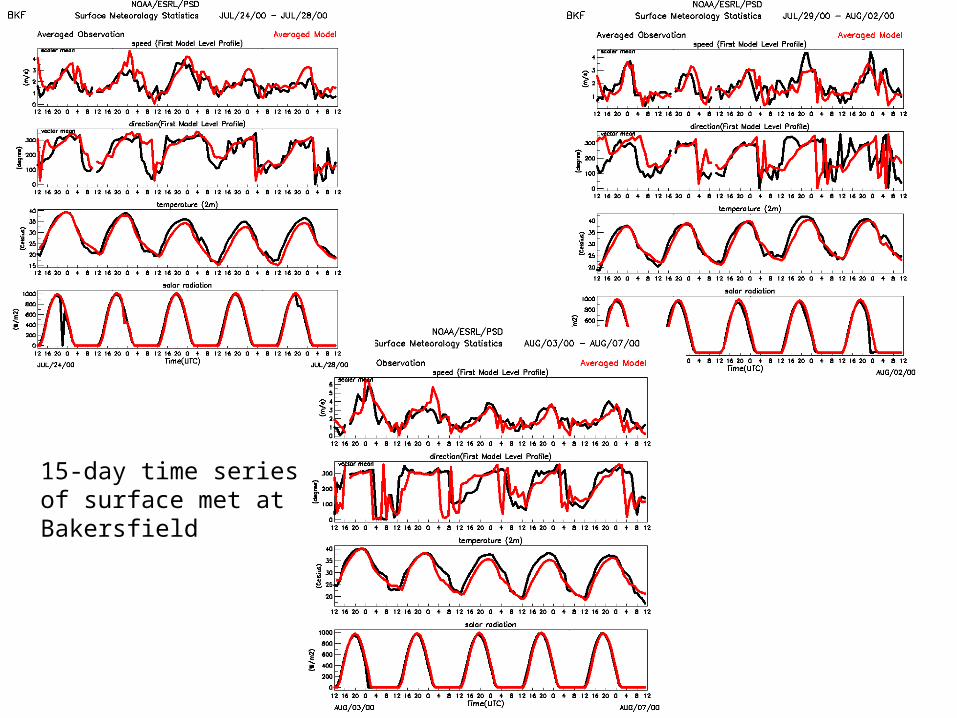
15-day time seriesof surface met atBakersfield

60% of observed winds required to plot a vector

30% for observed ABL depths

Richmond

Grass Valley

Redding

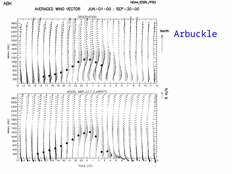
Arbuckle

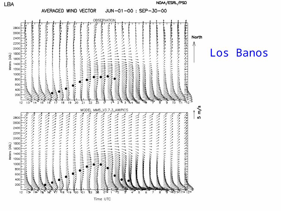
Los Banos

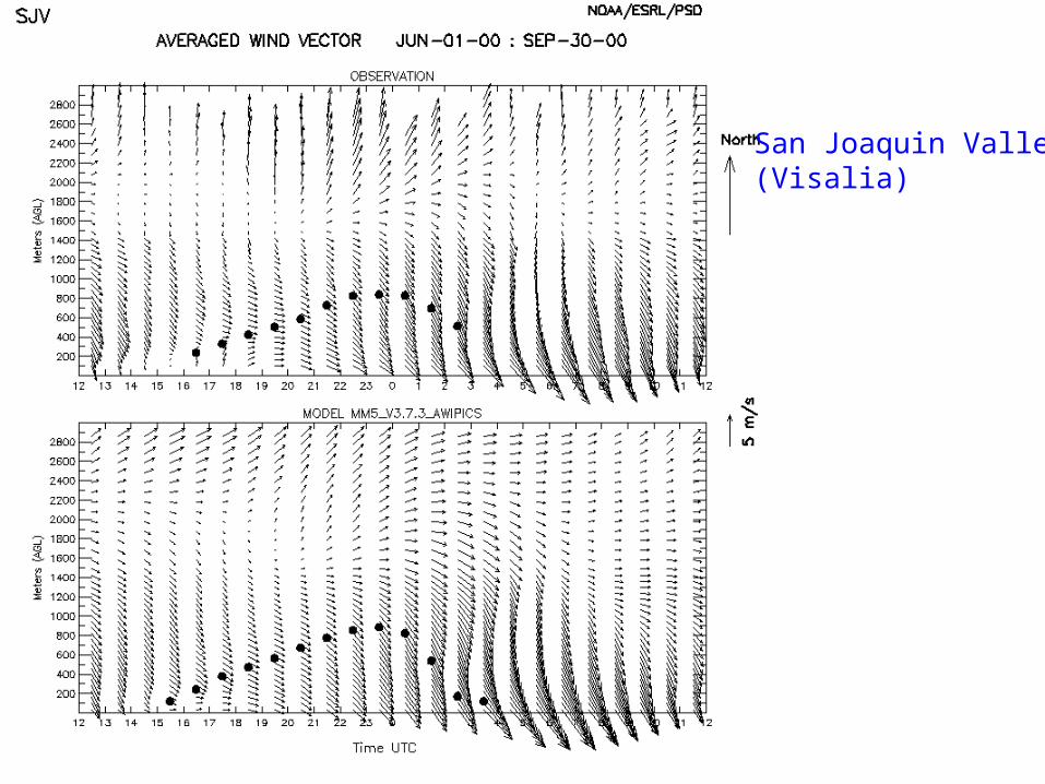
San Joaquin Valley(Visalia)

Bakersfield

Seasonal Modeling Summary

• Non-FDDA model replicates predominant “climatological” flow patterns at each profiler site

• Flow features reproduced include:– bifurcation of flow in the delta region– Nocturnal jet in San Joaquin Valley– Fresno and Schultz eddies– Timing of upslope/downslope along the Sierras– ABL depth magnitude and spatial variation

• Biggest shortcoming is that model underestimates southerly flow along eastern side of Sacramento Valley from SAC to RDG