1

Near-Field Acoustic Holography of a Vibrating Drum Head

Brendan Sullivan

University of Illinois at Urbana-Champaign

Dec. 18, 2008

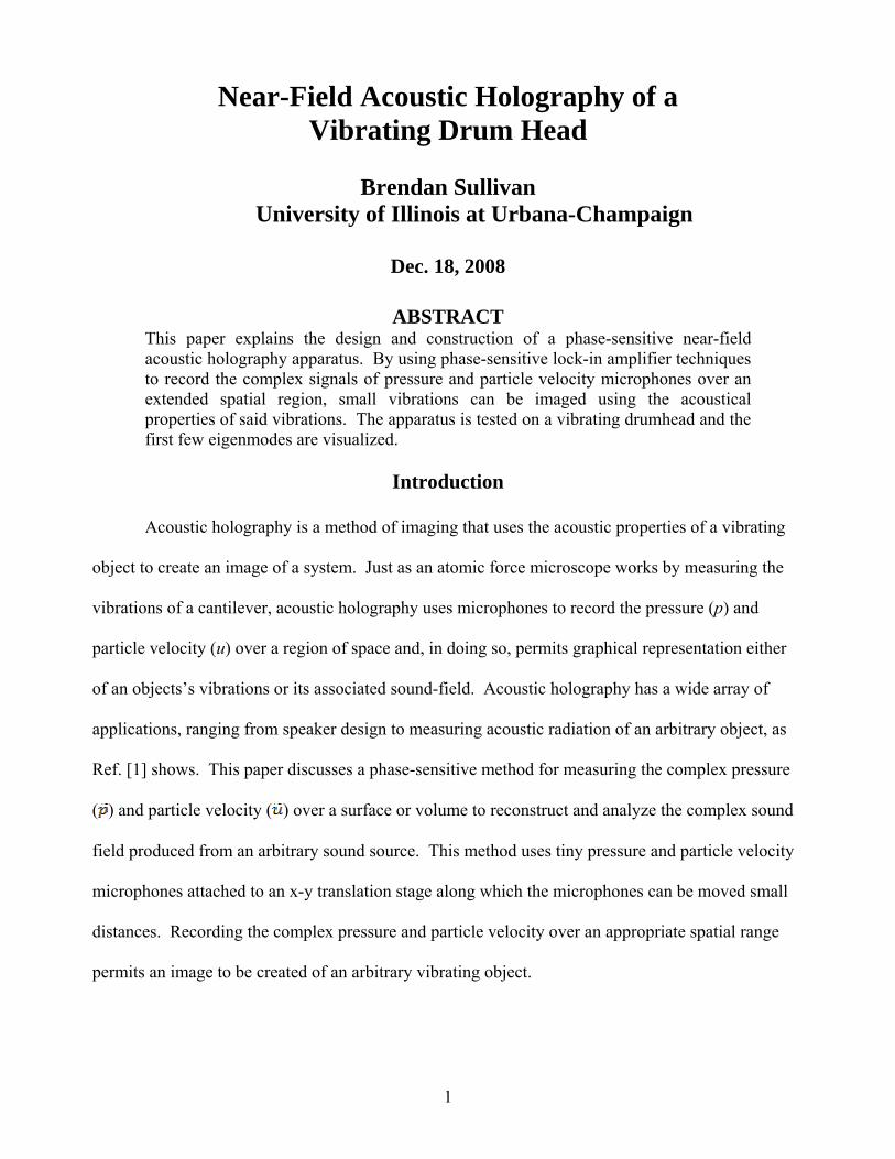
ABSTRACT This paper explains the design and construction of a phase-sensitive near-field acoustic holography apparatus. By using phase-sensitive lock-in amplifier techniques to record the complex signals of pressure and particle velocity microphones over an extended spatial region, small vibrations can be imaged using the acoustical properties of said vibrations. The apparatus is tested on a vibrating drumhead and the first few eigenmodes are visualized.

Introduction

Acoustic holography is a method of imaging that uses the acoustic properties of a vibrating

object to create an image of a system. Just as an atomic force microscope works by measuring the

vibrations of a cantilever, acoustic holography uses microphones to record the pressure (p) and

particle velocity (u) over a region of space and, in doing so, permits graphical representation either

of an objects’s vibrations or its associated sound-field. Acoustic holography has a wide array of

applications, ranging from speaker design to measuring acoustic radiation of an arbitrary object, as

Ref. [1] shows. This paper discusses a phase-sensitive method for measuring the complex pressure

( ) and particle velocity ( ) over a surface or volume to reconstruct and analyze the complex sound

field produced from an arbitrary sound source. This method uses tiny pressure and particle velocity

microphones attached to an x-y translation stage along which the microphones can be moved small

distances. Recording the complex pressure and particle velocity over an appropriate spatial range

permits an image to be created of an arbitrary vibrating object.

2

Fig. 1: The first 12 eigenmodes of a drumhead. Adjacent regions oscillate out of phase. For instance, in mode (0,1) the entire drum head moves in phase while in mode (1,1) the left and right side of the drumhead are 180° out of phase. Image modified from Ref. [2].

A vibrating drumhead was chosen to test the

apparatus. A drumhead is effectively a membrane

with clamped-edge boundary conditions, the theory

for which can be found in [2]. When a drumhead

resonates, its motion corresponds to superposition

of its eigenmodes (the first twelve of which are

shown in Fig. 1). By exciting the drumhead at an eigenfrequency corresponding to an eigenmode, it

is possible to directly observe each eigenmode and image the motion of air in proximity to the

drumhead.

Drumheads are not the only system this apparatus can measure. Measurements may be made

along different directions, allowing measurement of any arbitrary sound field. Another natural

candidate for testing with this apparatus, perhaps because of its similarities to a drumhead, is a

cymbal. It has been verified using optical holography that the eigenmodes of a cymbal form fractals

[3]. The fractal nature of a cymbal's eigenmodes should be observable using the same method as is

used to observe the eigenmodes of a drumhead. Additionally, this method could be expanded to

very accurately measure an arbitrary sound field, for instance the near and far-field acoustic

radiation from a loudspeaker.

In addition to offering the first phase-sensitive measurements of this kind, the microphones

associated with this apparatus can be placed much closer to the object. Typically measurements of

this sort are taken with a large array of microphones which effectively creates a surface above the

object. Placing this surface in proximity to the vibrating object can profoundly change the resulting

sound field, similar to the casing around speakers. Because the apparatus described below uses a

single pair of very compact microphones, they can be placed within a few millimeters of a vibrating

object without substantial sound field interference. Furthermore, it has been shown [4,5] that for a

3

planar object such as a drumhead that the sound field near the vibrating surface can be related to the

sound field at the vibrating surface. For a microphone located at a height above source the

plane can be described in the wave-number amplitude space. Using a standard fast Fourier

transform (FFT):

( ) ( ) ( ) ( ){ }, , , , , ,x yi k x k yx y m m mP k k z p x y z e dxdy FFT p x y z

+∞ +∞ +

−∞ −∞= ≡∫ ∫

( ) ( ) ( ) ( ){ }, , , , , ,x yi k x k yz x y m z m z mU k k z u x y z e dxdy FFT u x y z

+∞ +∞ +

−∞ −∞= ≡∫ ∫

Where and respectively represent pressure and the normal component of particle velocity

recorded by the microphones. In wave-number (k) space, there are two regions of interest. Inside

the radiation circle ( ), the values of p and u are taken to be the amplitude of the

respective wave. To mathematically translate the microphone from height to height

, a propagator, , is used:

( ) ( ), , , z p mik z zp m x yG z z k k e− −≡

With the density of air, c the propagation speed of the wave, and Δz the microphones’ distance

from the vibrating surface.

Once this is complete, the complex pressure and particle velocity at the vibrating surface are

given by the inverse FFT:

( ) ( ){ } ( ) ( ){ }1 1, , , , , , , , ,p x y p p m x y x y mp x y z FFT P k k z FFT G z z k k P k k z− −= =

( ) ( ){ } ( ) ( ){ }1 1, , , , , , , , ,z p z x y p p m x y z x y mu x y z FFT U k k z FFT G z z k k U k k z− −= =

Since particle displacement (i.e., the time integral of particle velocity, ) at the vibrating surface

must be the same as the vibrating surface’s displacement, the vibrating membrane can be imaged.

In addition to complex pressure, particle velocity, and displacement ( p ,u , and d ,

respectively), there are several other useful quantities to define. The simplest of these is

4

acceleration, the time derivative of particle velocity. The next is the longitudinal specific acoustic

impedance, pZ u= . The acoustic impedance is analogous to Ohm’s Law (with units of acoustical

Ohms) in electronics and is a property of the medium through which a sound wave is propagating.

The final substantial physical quantity is the complex sound intensity, *I p u= × which is related to

energy flow and work done by the sound field. The units of I are W / m2.

The rest of this paper describes the apparatus in more detail. The results given and exact

procedure are given for the study of drumhead motion, though this methodology could easily be used

on any other vibrating object.

Apparatus and Procedures

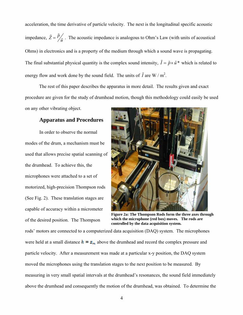
In order to observe the normal

modes of the drum, a mechanism must be

used that allows precise spatial scanning of

the drumhead. To achieve this, the

microphones were attached to a set of

motorized, high-precision Thompson rods

(See Fig. 2). These translation stages are

capable of accuracy within a micrometer

of the desired position. The Thompson

rods’ motors are connected to a computerized data acquisition (DAQ) system. The microphones

were held at a small distance above the drumhead and record the complex pressure and

particle velocity. After a measurement was made at a particular x-y position, the DAQ system

moved the microphones using the translation stages to the next position to be measured. By

measuring in very small spatial intervals at the drumhead’s resonances, the sound field immediately

above the drumhead and consequently the motion of the drumhead, was obtained. To determine the

Figure 2a: The Thompson Rods form the three axes through which the microphone (red box) moves. The rods are controlled by the data acquisition system.

5

phase relative to the driving function generator, the complex signal of each microphone was read via

a lock-in amplifier referenced to the function generator producing sine waves. A block diagram of

this setup is shown in Fig. 2b.

Figure 2b: A block diagram of the experiment with the electronics phase shift associated with each component. The magnets (black dot) are driven by the coil a la the NIC. The microphones under the drumhead are used to phase lock to a particular resonance while the top microphones are used to scan the drumhead in both the frequency and spatial scan modes. Since this is a phase-sensitive measurement, caution was used in calibrating the

microphones’ phase. Electronically, this was done in the same fashion described in Ref. [7].

The distance from the microphones to the also drumhead introduces a frequency-dependent phase

change, known as the propagation phase. The propagation phase can be found by holding the

microphone at a constant position in space (x0,y0,z0) near the drumhead and scanning frequency.

Then, barring all resonances, the phase should be constant. It was observed that over the ~ 0 Hz to 1

6

kHz range, both p and u had about a 36° phase change that was nearly linear with frequency. This

linear fit has been applied to the data given in this paper.

To extract physical quantities from the microphones, the microphones were absolutely

calibrated. After absolute calibration, output voltage from the microphone could be related to either

pressure or particle velocity, depending on the microphone. This was done using an Exetech

calibrator, which produces a Lp = 94 dB sound field. By definition,

= 94 dB

with p0 the pressure of free air, or at normal temperature and pressure (NTP). From

the above equation for Lp, it follows that the pressure of the sound field of 94 dB must correspond to

a pressure of 1 Pa. From the Euler equation, it can also be shown that a 94 dB sound field

corresponds to a particle velocity of 2.4 mm / s. By recording the output voltage of a microphone

exposed to a 94 dB sound field and relating that to the associated pressure and particle velocity, the

microphone values can be expressed in Pa or mm / s, rather than arbitrary volts.

To ensure that the amplitude of

the magnetic field driving the drumhead

was constant, a negative impedance

circuit (NIC) constant current driver was

placed between the function generator

and coil. Since the magnetic field of the

coil is linearly proportional to current

through the coil, I, it had to be ensured

that the current amplitude, not voltage,

remained constant with frequency.

Figure 4 shows simulation data on the circuit’s behavior. The branch $10, shown in purple,

Figure 3: The constant current NIC for the driver coil. This circuit ensures that the magnets amplitude is constant.

7

represents current amplitude through the coil. In the region of interest, f << 10 kHz, the coil’s

current exhibits flat response in both magnitude and phase, as is required of this circuit.

Because the location of the magnet is, by necessity, an anti-node on the drumhead, it’s

longitudinal motion can be modeled as a damped, driven harmonic oscillator with the equation of

motion ,z magnetmz m z kz Fγ+ + = . m here represents the mass of the magnets and drumhead clamped

by the magnets, γ the drumhead’s damping coefficient, and Fz,magnet is the longitudinal component of

force on the magnets from the coil. Treating the two magnets as a pure magnetic dipole with

moment magm , the force can be expressed as

( ) ( ) ( ) ( ) ( ) ( ) ( )

( ) ( )( )( )

( )

2,1=

c

, , , ,

, ,

coil

mag mag coil mag coil coil mag

mag coil coil mag

E r tt

F r t m r B r t m r B r t B r t m r

m r B r t B r t m∂

∂

⎡ ⎤= ∇ = ∇ + ∇⎣ ⎦

+ × ∇× + × ∇×

i i i

( )( )r

Once the calibrated data was

taken, a surface was drawn over spatial

coordinates and various acoustical

properties. This was done using an

MATLAB m-file that first formed a

mesh-grid of all the coordinates where

data was taken and then plotted a three

dimensional surface of the quantities

measured. This surface, when

measured at one of the drum’s

resonances, emulates the normal modes shown in the motivation section of this paper, confirming

the experimental observation of the drum’s eigenmodes.

Figure 4: Frequency response of the NIC circuit. The current amplitude through the coil is given by $10, the purple line. In the region of interest (<<10 kHz) the response is flat in both magnitude and phase.

8

Because resonances of drumheads have a strong

temperature dependence, a mode-locking system had to be

installed in the apparatus. When the drum is vibrating on an

eigenmode, the pressure directly underneath the magnet will

be extremal and entirely imaginary (one of the red dots in Fig.

5). Consequently, a pair of mode-locking pressure and

particle velocity microphones were placed underneath the

drumhead and the desired resonance was found. Ambient

temperature drift lead to a drift in resonance frequency, so the

excitation frequency was tweaked between scanning points until the imaginary component of

pressure was at an extremal point, shown in Fig. 5. The frequency is set by hand to be between flo

and fhi. Then, between scanning points the frequency is tweaked, which effectively shifts the

pressure along the blue curve in Fig. 5, until the resonance is found again (the red dot). It is worth

noting that if the temperature changes too drastically or the mode-locking system overshoots its

target by too much (i.e. goes beyond flo or fhi) then the mode has been lost and the current scan must

be discontinued. The typical variation is around fhi - flo = 1 Hz.

Results and Analysis

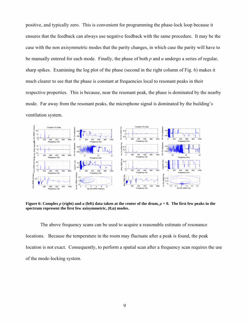
The results of a typical axisymmetric frequency scan are given in Fig. 6. There are several

noteworthy features in these plots. First, since this was taking with the microphones at the center of

the drum, the first few peaks in each spectrum indicate the first few (0,n) modes. That is to say, the

first peak in p represents the (0,1) mode as determined by p, the second peak is the (0,2) mode, and

so on. Additionally for these peaks, the parities of pressure are all the same. For example, the real

part of the pressure will fall before it hits a maximum, while the imaginary component is always

Figure 5: To compensate for the eigenfrequency drift due to temperature, the frequency is shifted between scanning points until pressure falls on one of the two red dots above.

9

positive, and typically zero. This is convenient for programming the phase-lock loop because it

ensures that the feedback can always use negative feedback with the same procedure. It may be the

case with the non axisymmetric modes that the parity changes, in which case the parity will have to

be manually entered for each mode. Finally, the phase of both p and u undergo a series of regular,

sharp spikes. Examining the log plot of the phase (second in the right column of Fig. 6) makes it

much clearer to see that the phase is constant at frequencies local to resonant peaks in their

respective properties. This is because, near the resonant peak, the phase is dominated by the nearby

mode. Far away from the resonant peaks, the microphone signal is dominated by the building’s

ventilation system.

Figure 6: Complex p (right) and u (left) data taken at the center of the drum, ρ = 0. The first few peaks in the spectrum represent the first few axisymmetric, (0,n) modes.

The above frequency scans can be used to acquire a reasonable estimate of resonance

locations. Because the temperature in the room may fluctuate after a peak is found, the peak

location is not exact. Consequently, to perform a spatial scan after a frequency scan requires the use

of the mode-locking system.

10

As mentioned before mentioned, the

phase observed by the reference microphone

should be a constant 90° or -90°. Figure 7

shows the reference phase as a function of

measurement number. The phase is roughly

locked at the desired -90°. To further

demonstrate the effect of the mode-locking

setup, the resonant frequency as a function of

measurement number is given in Fig. 8.

In an ideal system, the frequency

would be constant, and determined solely by

the geometry of the system. However,

temperature variations cause a drift in the

resonant frequency of the drum.

A spatial scan of the drumhead

unambiguously reveals the mode. Figure 9

shows data for the (0,1) resonance mode and

Fig. 10 shows the (0,2) mode. Note that

since Re(P) and Im(U) are zero across the

head, they are omitted.

Figure 7: Reference phase versus measurement number. The reference phase is roughly a constant -90 except for the spikes to 0. These spikes are an artifact of the measurement, and represent the phase of free air (arbitrarily taken to be zero).

Figure 8: Sample frequency as a function of measurement number. In an ideal system the resonant frequency would be constant throughout the measurement. However, drifts in ambient temperature lead to drifts in resonant frequency.

11

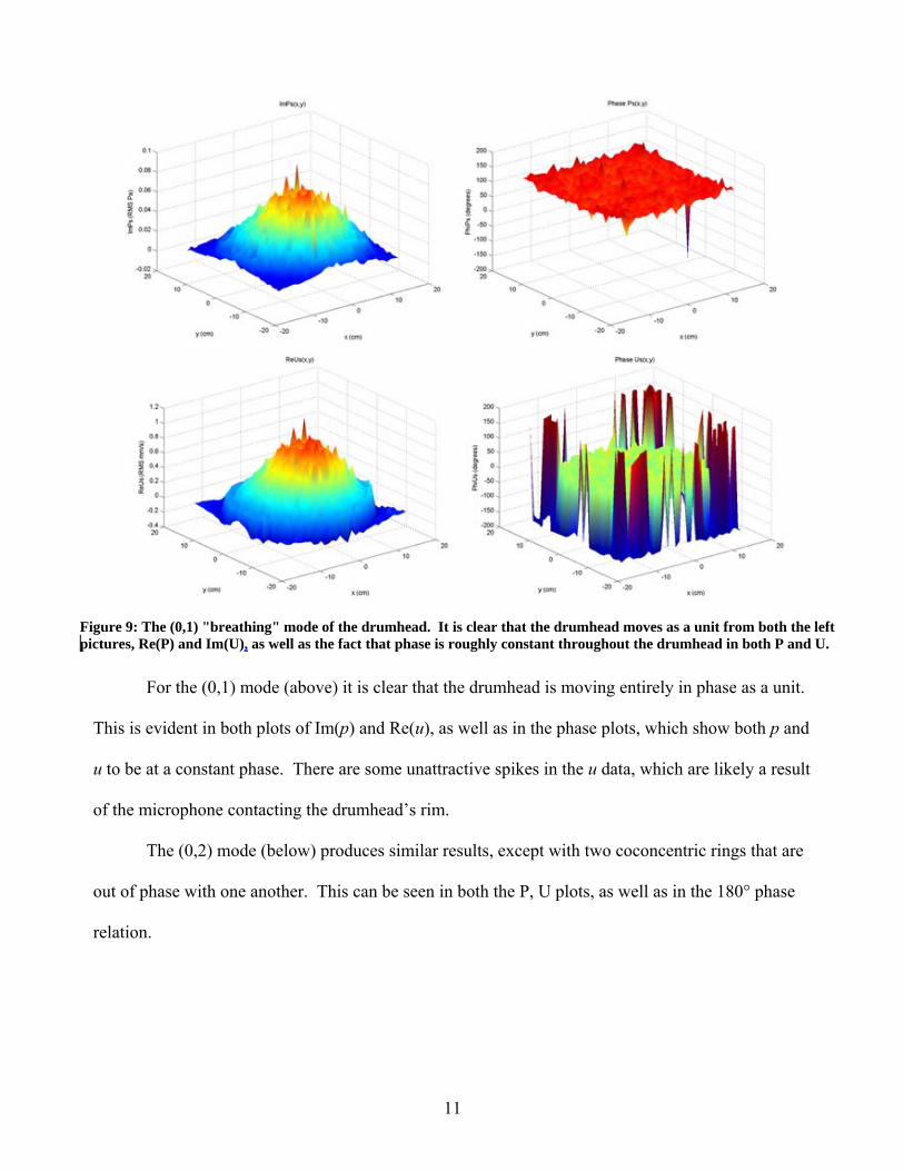
For the (0,1) mode (above) it is clear that the drumhead is moving entirely in phase as a unit.

This is evident in both plots of Im(p) and Re(u), as well as in the phase plots, which show both p and

u to be at a constant phase. There are some unattractive spikes in the u data, which are likely a result

of the microphone contacting the drumhead’s rim.

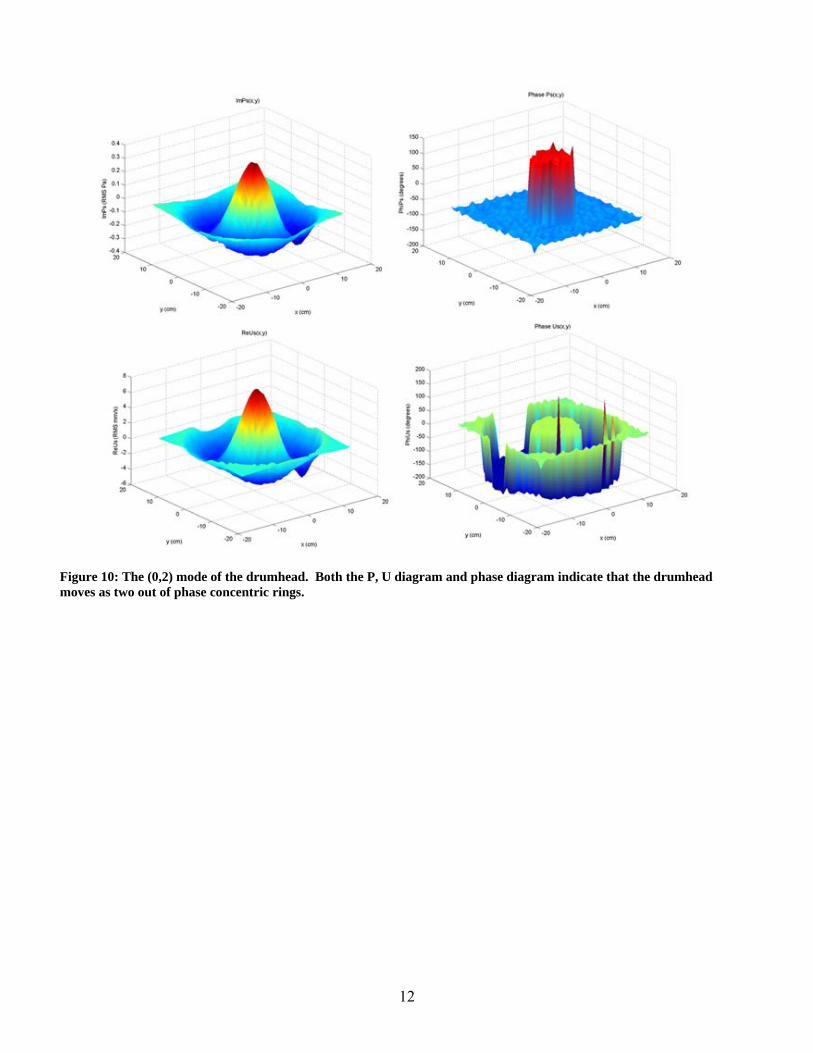
The (0,2) mode (below) produces similar results, except with two coconcentric rings that are

out of phase with one another. This can be seen in both the P, U plots, as well as in the 180° phase

relation.

Figure 9: The (0,1) "breathing" mode of the drumhead. It is clear that the drumhead moves as a unit from both the left pictures, Re(P) and Im(U), as well as the fact that phase is roughly constant throughout the drumhead in both P and U.

12

Figure 10: The (0,2) mode of the drumhead. Both the P, U diagram and phase diagram indicate that the drumhead moves as two out of phase concentric rings.

13

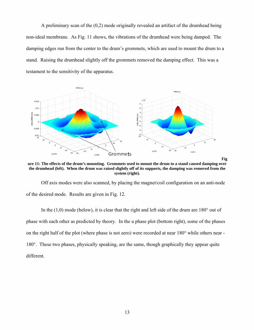
A preliminary scan of the (0,2) mode originally revealed an artifact of the drumhead being

non-ideal membrane. As Fig. 11 shows, the vibrations of the drumhead were being damped. The

damping edges run from the center to the drum’s grommets, which are used to mount the drum to a

stand. Raising the drumhead slightly off the grommets removed the damping effect. This was a

testament to the sensitivity of the apparatus.

Figure 11: The effects of the drum’s mounting. Grommets used to mount the drum to a stand caused damping over the drumhead (left). When the drum was raised slightly off of its supports, the damping was removed from the

system (right).

Off axis modes were also scanned, by placing the magnet/coil configuration on an anti-node

of the desired mode. Results are given in Fig. 12.

In the (1,0) mode (below), it is clear that the right and left side of the drum are 180° out of

phase with each other as predicted by theory. In the u phase plot (bottom right), some of the phases

on the right half of the plot (where phase is not zero) were recorded at near 180° while others near -

180°. These two phases, physically speaking, are the same, though graphically they appear quite

different.

14

Figure 12: The (1,0) eigenmode. The left and the right side are 180° out of phase with each other. For the phase of u, it should be noted that on the right side, some points were found to have phases of 180° while others had -180°. In the complex plane, these two are equivalent, though graphically they appear to be quite different.

Though other modes were scanned, it is not necessarily fruitful to include them in the report.

For those interested, all plots from scans taken will be available on the UIUC P199POM and

P498POM websites in Adobe PDF form [9].

15

Discussions and Conclusions

This paper describes a phase-sensitive machine for acoustic holography. For several reasons

it was tested by observing the eigenmodes of a vibrating drumhead. However, the apparatus was

developed generally so that it can be used to map the sound field of any vibrating object.

The applications of a general acoustic holography machine range from geophysics to large

scale auditorium and stadium design and instrument design. For instance, the damping observed by

the drum’s mounting is perhaps an effect the drum maker did not have the technology to observe.

Acoustic holography is also a widely used in determining the internal contents of a rock [8],

particularly in an effort to fine more oil. Though it is currently done only with magnitudes, the

inclusion of phase may lead to a more fundamental standing of the acoustical properties of

geological materials.

Acknowledgements

I would like to acknowledge, above all, my advisor Professor Steven Errede. I would also

like to thank Nicole Pfeister (Purdue University) and Marguerite Brown (University of Chicago) for

their shared workspace over the summer. This work was made possible through a grant from the

Shell Oil Foundation through the Physics Department at the University of Illinois at Urbana-

Champaign.

16

References

[1] ─ Sean F. Wu, Nassif Rayess, and Xiang Zhao, J. Acoust. Soc. Am. 109, 2771-2779. (2001).

“Visualization of acoustic radiation from a vibrating bowling ball.”

[2] ─ T.D. Rossing, The Physics of Musical Instruments (1973).

[3] ─ Staffan Schedin, Per O. Gren, and Thomas D. Rossing, J. Acoust. Soc. Am.103, 1217-1220.

(1998). “Transient wave response of a cymbal using double-pulsed TV holography”

[4] – Finn Jacobsen and Yang Liu, “Near field acoustic holography with particle velocity

transducers,” J. Acoust. Soc. Am. 118 (5), 2005.

[5] – S. Errede, “Near-Field Acoustic Holography,” (unpublished).

[7] – D. Pignotti, “The Acoustic Impedance of a B-flat Trumpet,” Senior Thesis, (unpublished)

[8] – Oscar Kelder and D.M.J. Smeulders, Geophysics 62, 6, 1794-1796, (1997). “Observation of

the Biot slow wave in water-saturated Nivelsteiner sandstone”.

[9] – http://online.physics.uiuc.edu/courses/phys199pom/199pom_reu.html and

http://online.physics.uiuc.edu/courses/phys498pom/498pom_reu.html