Embed Size (px)
Citation preview

NBER WORKING PAPER SERIES
SELECTION AND IMPROVEMENT: PHYSICIAN RESPONSES TO FINANCIAL INCENTIVES
Jason BarroNancy Beaulieu
Working Paper 10017http://www.nber.org/papers/w10017
NATIONAL BUREAU OF ECONOMIC RESEARCH1050 Massachusetts Avenue
Cambridge, MA 02138October 2003
We want to thank John Shin for his help with the early stages of this project. We also thank George Baker,David Cutler and seminar participants at Kellogg School of Management, Case Western, Boston University,Harvard University and MIT for their helpful comments. We are appreciative to all HCA, The HealthcareCompany employees who provided us insight and data. All errors are our own. The views expressed hereinare those of the authors and are not necessarily those of the National Bureau of Economic Research.
©2003 by Jason Barro and Nancy Beaulieu. All rights reserved. Short sections of text, not to exceed twoparagraphs, may be quoted without explicit permission provided that full credit, including © notice, is givento the source.
Selection and Improvement: Physician Responses to Financial IncentivesJason Barro and Nancy BeaulieuNBER Working Paper No. 10017October 2003JEL No. I1, J3, L3
ABSTRACT
In this study we examine the effects of transferring physicians from a compensation system based
on salary to a profit-sharing system. Consistent with theory, we find that the change has a large and
significant effect on the quantity of services provided. In addition, we find a selection effect, where
the least productive doctors leave the company and more productive doctors join.
Jason BarroHarvard Business SchoolBaker Library 184Boston, MA 02163and [email protected]
Nancy Beaulieu Harvard Business SchoolBaker Library 284Boston, MA 02163and [email protected]

1
Introduction
Economists are fond of writing down models in which employees are paid a wage based
on their productivity. However, with the exception of executive compensation studies, there are
few documented cases of such pay practices. The most well known of these studies (Lazear,
2000) finds very substantial productivity effects (20% to 36% of output) and positive selection
effects among auto windshield installers. Lazear speculates that piece rate pay may not have the
same productivity and profitability effects for managerial and professional workers, perhaps
because of the difficulty of measuring output and detecting and assigning quality problems in
these jobs. In this paper, we investigate the response of physicians to a particular form
productivity pay – profit sharing.
Analyzing a unique data set provided by a large hospital company (HCA, The Health
Care Company) that employed physicians, we find that the institution of performance-based pay
in Florida had three main effects. First, the doctors that were switched from salary to the profit-
sharing plan increased their profitability significantly, primarily through increases in output.
Second, the least productive doctors left the company. And third, after implementing the profit-
sharing plan, the company attracted new doctors who were more productive on average than the
doctors employed previously under the salary contracts.
The paper is organized as follows. In the next section, we set the context for our study by
summarizing changes in the healthcare market that precipitated hospital ownership of physician
practices. We then briefly summarize the literature on physician pay practices and Lazear’s paper
on productivity pay. In section three, we present the theoretical underpinnings for our empirical
analyses and in section four we present the results of our empirical analyses. The final section
concludes and suggests an outline for future research.

2
The Healthcare Context
Throughout the last century, most physicians were self-employed in solo practice. Up
until the 1990s, the typical contract between an insurer and a physician was based on fee-for-
service payment, in which the physician and the patient decided what care was appropriate and
the doctor was reimbursed ex-post, according to an agreed upon fee schedule, for the care
provided. Under that system, health care costs and insurance premiums grew at a rapid pace.
Consumers and their employers fought the increased premiums, and this led insurance companies
to develop new techniques for controlling costs. The manifestation of these new techniques was
embodied in the rapid rise of managed care companies during the decade of the 1990s.
From the standpoint of the physician, these changes in the insurance industry made the
old model of the independent solo-practice unattractive. First managed care companies began to
introduce much more sophisticated reimbursement contracts that utilized payment mechanisms as
instruments to control costs. Physicians were increasingly being asked to bear financial risk for
the cost of delivering health care services under the insurance contract; solo practitioners were ill-
suited to bear much of this risk because of natural limits on panel size and because of the heavily
skewed distribution of medical costs. Second, managed care companies also began to assert
bargaining power in negotiating reimbursement rates with physicians. As solo-practitioners with
patients from many different insurance companies, most physicians did not have the clout to stave
off fee reductions.
In response, doctors in many markets re-organized to better position themselves to
contract with managed care companies. In some cases, physicians formed medical group
partnerships; in other cases, physicians affiliated with an intermediary solely for purposes of
contracting with insurance companies (Robinson, 1999). Today, in most markets, there exists a
contracting intermediary between the insurance company and the doctors that deliver care, and
that organization must decide how to compensate physicians. Occasionally, a hospital serves this
3
intermediary role; this is the organizational context for our study of physician pay practices
presented in this paper.
At the same time that managed care companies were altering physician pay practices,
they were also reducing the number of hospital admissions and shortening the average length of
stay for those patients who were admitted. In many markets, these reductions in hospital
utilization led to excess capacity in hospitals. Hospitals felt pressure to compete for an ever-
shrinking base of potential patients. Purchasing physician practices became one of the critical
components of the hospitals’ strategies to ensure patient flows. As Jamie Robinson writes in his
book on physician organization:
“The hospital is a business with high fixed and low marginal costs for whom the incremental patient admission is very valuable. Hospitals are fundamentally dependent on their affiliated physicians for patients and hence for revenue, yet historically have found it difficult to cement their relationships. The acquisition of physician practices is merely another facet of this effort, the acquisition of a future stream of hospital admissions (p. 181).” Historically, doctors and hospitals contracted separately (and independently) with
insurers. Doctors applied to hospitals for admission privileges, but these privileges were granted
independently of the doctor’s contracts with managed care companies. Thus, doctors and
hospitals had a rather symbiotic relationship but this relationship did not involve a legal contract
(with regards to delivery of or payment for services).
When a hospital purchased a physician practice, the only tangible capital it acquired was
the practice’s physical plant and equipment. The doctors (and their staff) typically became
employees of the hospital and were paid a flat salary. The hospital then negotiated contracts with
managed care companies and became the residual claimant on the practice’s profits. Note
however, that the hospital in no way “owned” the doctors’ patients. The hospital was, and is,
prohibited by law from limiting the set of hospitals to which its doctors may admit patients.
Thus, while hospitals could not use ownership of physician practices to assure patient
flows, it is widely acknowledged that this is the outcome the hospitals hoped to secure.

4
From the hospital’s perspective, it might still make financial sense to purchase a physician
practice even if the hospital loses money on the practice itself. These operational losses might be
offset by increased admission revenues.
In the sections that follow, we examine the effect of profit-sharing contracts on physician
behavior at a single hospital company. This study cannot address the issue of whether hospitals
should employ doctors, because we do not observe hospital admissions and thus cannot measure
the effect of said patient flows on hospital profitability. While we find the questions of vertical
integration and the optimal organizational boundaries of the hospital very interesting, we are
unable to study these problems with the data available for this study.
Literature Review
There has been some empirical literature examining the question of whether physicians
change their behavior in response to financial incentives. In a study of for profit ambulatory care
centers that switched their physician compensation method from salary to productivity pay based
on net income, Hemenway et al. (1990) find evidence that physicians’ productivity responds
positively to financial incentives. All physicians, regardless of whether they qualified for the
productivity pay or not, increased their monthly charges by an average of 20 percent after the new
compensation program was put in place. The increases in charges were the result of increases in
services provided per patient visit and increases in the number of office visits per month. Six of
the fifteen physicians in this study generated enough monthly charges to qualify for the
productivity pay in every month of the study.
Barro et al. (2003) found substantial productivity effects in a small group of orthopaedic
surgeons when the group converted to a compensation plan in which each surgeon’s semi-annual
bonus was calculated as a fixed percentage of the profits the surgeon generated. In one year’s
time, nearly all of the surgeons increased the number of surgeries performed (an explicit objective
of the compensation plan) though only 24% of the physicians increased their profits. Gaynor and

5
Pauly (1990) examine free-rider effects and the responsiveness of individual members of medical
group practices to productivity pay. Here also, the authors found that physicians’ productivity
(measured in number of office visits) responded positively to financial incentives.
In a different setting, Lazear (1996) examined selection and productivity responses
among auto glass installers who were given the option to participate in an incentive pay program.
The wage agreement involved a wage guarantee combined with piece rate incentives designed to
increase productivity. The employees were paid by piece rate when their productivity pay
exceeded the guaranteed wage and were fired if their output fell below some minimally
acceptable level. This compensation arrangement is equivalent to a guaranteed salary with a
minimum output requirement and a productivity bonus for output exceeding the minimum
requirement. 1 Lazear’s model predicts three behavioral responses to the imposition of
productivity pay. First, the model predicts that output under piece rates will be greater than or
equal to output under salary. Output will be strictly higher under piece rates when the firm sets
the linear component of the piece rate contract sufficiently high such that the optimal effort for
some workers under the piece rate contract exceeds the minimum required for continued
employment. The second result predicts that if some workers choose the piece rate and some
workers choose the guaranteed salary, the average ability of the people employed by the firm will
rise (i.e. a positive selection effect). Finally, the third result predicts that the variance of ability
and output will rise if some workers choose the piece rate and some workers choose the
guaranteed salary.
The empirical analysis generates confirming evidence for all three of the model’s
predictions. In particular, the author finds that on average, an employee’s pay increased by 9.6%
and that productivity increased by 20% under the new compensation scheme; thus employees
captured roughly half the gains of the returns from their productivity increases. The author also
1 The empirical counterpart to effort in Lazear’s model is observed output. Thus effort and output are used interchangeably in what follows.
6
finds a decrease in employees’ use of sick leave and that the piece rate scheme works to select
employees who are less likely to take sick leave. Two possible reasons for the success of this
piece rate system are the observability of the output on which compensation was based and the
easy detection and assignment of quality problems. Lazear speculates that managerial and
professional jobs may not be as well suited to piece rate pay, presumably because of the lack of
outcome observability and the difficulty with assessing and attributing the quality of the product.
Model
The model put forth in this paper is an adaptation to the model developed by Lazear
(2000). The changes are necessary to accommodate differences between the compensation
scheme in the Lazear model and the compensation scheme offered to employees in the physician
data we analyze. In the firm we study, employees were not offered a wage guarantee when the
firm switched to productivity-based pay. The absence of a wage guarantee requires us to
generalize the model described above to obtain predictions on employee output and ability levels.
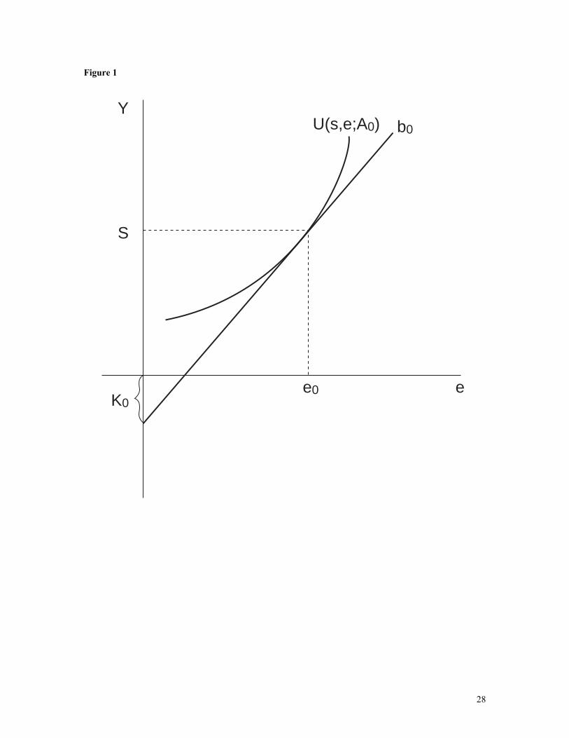
Consider a firm that employs workers for a salary, si, and requires some minimum level
of effort from the worker, e0. In practice, effort cannot be observed by the employer; but output
can be observed and is assumed to be some monotonically increasing function of effort. The
employee’s utility function is given by:
Ui (Y, e) = Yi – C(e) / Ai
where Ai is the innate ability of the employee which reduces the employee’s cost of effort
required to produce a given level of output. Ability is distributed in the population according to
the distribution function F(Ai). Income, Yi, is wage income and equal to si if the individual is
employed under a salary contract. We assume there exists a diverse set of job opportunities

7
present in the economy and the combination of these opportunities and the worker’s ability
generates a reservation utility, R(Ai), for each worker. The reservation utility is the utility the
worker would derive from his or her most attractive job alternative and is assumed to be linear in
the worker’s ability (R’(Ai)>0). Under these assumptions, the worker will accept a salary
contract if and only if her utility exceeds R(Ai) when ei > e0. Under this contract, the rents (si –
C(e) / Ai - R(Ai)) if any, are captured solely by the worker.2
Under a linear piece rate contract (wages = b*ei + K), the employee chooses effort to
maximize utility; this level of effort equates marginal benefit from increased effort with marginal
cost (i.e., e is chosen such that b = C’(ei*)/Ai). Whether or not the employee will enter into the
piece rate contract depends on whether utility from the piece rate contract exceeds the employee’s
reservation utility.
Let (b0, K0) be the productivity-based employment contract that leads the lowest ability
worker under salary (A0,sal) to generate the same output (e0) and obtain the same utility as under
the salary contract. An example of such a contract is illustrated in Figure 1 and given by:
b0 = C’(e0*) / A0 where e0* = e0
k0 = s - b0e0*
Proposition 1: For Ai ∈ (Ao, pr, Ah, pr], k = k0 and b > b0,
ei, pr > ei, sal .
2 For the population of employees that we will study, it is plausible that some individuals will possess an ability level such that they would earn rents under the salary contract offered by the firm. However this subset of workers may not earn any rents (or earn lower rents) in practice if they subscribe to a norm that establishes a minimum level of effort, enorm , that is higher than the threshold effort e0 required under the salary contract.

8
Proof: See the appendix for a formal proof. From Figure 2, note that the tangency of the
indifference curve to b0 for any Ai > A0 will occur to the right of e0, since dU /
dA < 0 for a given contract (b0, k0). Also note that for all Ai > A0 , Ui (e0; s) < Ui
(ei*; b0, k0).
The above proposition states that if the lowest ability worker chooses to remain with the
firm under a piece rate contract that elicits the same output as under salary, then output will
increase for all employees with higher ability levels who also accept the piece rate contract. The
set of workers who will be employed under the piece rate contract [Ao,pr Ah,pr ] is a function of the
generosity of the piece rate contract and the employees’ reservation utilities.
Let R(A) be linear in A and define H(Ai) to be the utility that the individual with ability i
derives from the salary contract (H(Ai) = s – C(ei) / Ai). In Figure 3, the range of ability among
workers employed by the firm under the salary contract is [Ao,sal Ah,sal ]. Define G(Ai) to be the
utility that the individual with ability i derives from the piece rate contract (b0, k0): G(Ai) = b0 ei*
– C(ei*) / Ai. Recall that the linear piece rate contract was chosen such that utility under the two
contracts is equal for the lowest ability worker, G(A0) = H(A0). It is relatively straight-forward to
show that this piece rate contract will attract higher ability workers.
Proposition 2: For the linear piece rate contract (k0, b0),
Ah,sal < Ah,pr
Proof: See the appendix for a formal proof. From Figure 3, G(Ai) must lie every above
H(Ai) for Ai>A0,sal since G’(Ai)>H’(Ai) in this range for the contract (b0, k0).
Thus H(Ah,sal) = R(Ah,sal) < R(Ah,pr) = G(Ah,pr) and since R’(A) >0, Ah,sal < Ah,pr.

9
Proposition 2 states that the piece rate contract that retains the lowest ability worker
under salary will also attract higher ability workers to the firm. Thus, the imposition of the piece
rate contract (b0, k0) results in two separate productivity enhancing effects for the firm: (1)
individual productivity increases for everyone employed under the piece rate system except the
lowest-ability worker (proposition 1 – the improvement effect); and (2) the productivity-based
contract attracts higher ability workers to the firm (proposition 2 – the selection effect).
Whether or not the piece rate contract (b0, k0) is optimal from the firm’s point of view
will depend on the distribution of ability in the population of potential employees and the
marginal product of labor. The firm can select a different pool of workers by altering the two
components of the wage contract. For example, as shown in Figure 4, the firm can attract a pool
of employees with a smaller (or greater) range in ability by lowering (or raising) k0. Similarly,
the firm can attract more (or fewer) high ability employees by raising (or lowering) b0 (see Figure
5).
Data and Background on Study Site
At the time of this study, HCA was the nation’s largest, for-profit hospital company. At
its peak in 1986, HCA owned 486 hospitals nationwide. Along with many other hospitals, both
not-for-profit and for-profit, HCA began to aggressively purchase physician groups in the early
1990s. By 1998, HCA employed over 2000 physicians.
When HCA purchased a physician group, the doctors in the practice were given a large
cash sum plus a guaranteed annual salary. In addition, HCA took over responsibilities for
negotiating contracts with insurers. HCA’s primary financial consideration may have been the
patient flows to hospitals. In fact, HCA appeared so unconcerned with the financial performance
of individual practices, that their financials were buried in the financial statements of the nearest
hospital. In 1997, HCA changed the financial reporting standards for its physician practices.
Each practice, and soon, each physician, was tracked with separate financial statements. Once

10
HCA began to examine the numbers, they came to realize that HCA was losing roughly $100
million per year on the practices.
HCA officials, with whom we have spoken, contend that, until 1997, they did not know
whether or not the practices were losing money. Furthermore, company executives did not
anticipate that doctors would alter their behavior towards their patients very dramatically in
response to the form of their compensation.
HCA’s experience was similar to many physician-hospital organizations around the
country. In his case study of the St. Joseph Hospital System in Orange County in California,
Jamie Robinson reports the experience of the physician hospital organization (the St. Jude
Heritage Health Foundation) that bought several medical groups in an attempt to retain market
share:
“… the Foundation had felt the need to provide a safety net under physician earnings to convince them to go along with the sale. Income guarantees are notorious, however, for undermining the subsequent productivity of the physicians. The effects of income guarantees were compounded by the newfound wealth of many Bristol Park physicians, who now wanted to work shorter hours and take longer vacations to enjoy their gains (p. 186).” Even if HCA was not in the physician practice business to make money from the
practices, themselves, HCA did not want to lose a substantial amount of money. The company
immediately took steps to stem its losses by ceasing its acquisition strategy, and increasing
oversight of the practices. In the months that followed, the executives at HCA decided that
financial incentives, or the lack of them, may have been a critical contributor in the financial
shortfall. As a consequence, in 1998 they began to implement a new compensation system called
Pre-Comp Earnings (PCE).
Under PCE, the physician practice paid HCA a fixed management fee of roughly
$3,000/month per physician. After the management fee, the practice shared profits with HCA;
physicians retained 85-95% of the profits. Under PCE, the physician practice thus became a profit
center, and the doctor’s take-home pay became a fixed percentage of the profits generated by the

11
practice. If the practice lost money, the doctor owed HCA the full amount of the loss – so HCA
did not share in the risk of losses. In the early stages of implementing the PCE program, HCA
made “loans” to the doctors (which they were required to repay) to smooth the transition to profit-
sharing.
As salary contracts expired, HCA transferred doctors onto the PCE system. Since some
doctors had long-term contracts with guaranteed salaries, not all doctors were switched onto PCE
at the beginning of the program. We have no reason to believe that the order in which these
salary-based contracts were negotiated in the first place (and hence the order in which practices
were transferred to PCE) is in any way related to the performance of the practices once on PCE.
In other words, we do not believe that a selection effect in the assignment of practices to the
treatment group (the practices that switch to PCE) will bias our results.
The data we use in our analyses are monthly financial data from HCA’s Florida physician
practices over the period January 1998 to December 1999. The sample includes data for 72
physician practices, comprised of 140 doctors. The median practice contains only one doctor and
the maximum contains seven. The data contains information on the revenues generated by the
practice as well as detailed cost information.
During the time period of our analysis, HCA officials have told us that the reimbursement
agreements with insurance companies were relatively stable. More importantly, there was no
systematic correlation between the transition of any doctors onto PCE contracts and the
renegotiations of any contracts with insurance companies. We therefore interpret any changes in
revenues to be the result of changes in quantities of services provided and not changes in prices.
Note that changes in the quantities of services provided can result from several different
behavioral changes, including increased effort, or simply a reshuffling of services provided from
poorly-reimbursed activities to more highly-reimbursed activities. With our financial data, we are
unable to identify the proximate causes of changes in quantities of services provided.

12
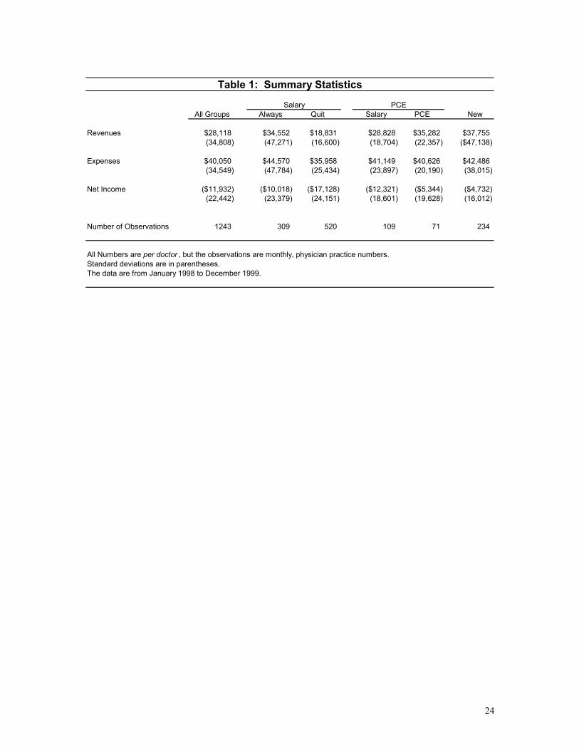
Table 1 presents some summary statistics for the entire sample of practices, as well as for
several important subgroups. Out of the 72 physician groups in the Florida data, 12 spend some
portion of the sample period under PCE, with transition dates staggered over the time period. We
divide groups into four categories: (1) practices that spent some time on PCE during the sample
(12 groups, 3 are newly-hired), (2) those that are always on salary (13 groups) and remain with
HCA during the entire sample period, (3) those that are always on salary but terminate their
contract with HCA during our sample period (32 groups), and (4) those that were hired during the
sample period and do not start on PCE (15 groups). The groups that were hired after the
beginning of 1998 did so with the understanding that they would eventually be compensated
under PCE, so in terms of selection issues this group merits a separate evaluation. In Table 1, the
3 practices that are new and began under PCE are included with the other new practices and are
not included with the PCE averages.
Support for the three basic empirical hypotheses we test in the regression analysis are
apparent from this table of averages. First, the groups that switch onto PCE perform significantly
better under PCE than they did under salary. Net income increases significantly and this increase
is generated almost entirely through a 21% average increase in revenues ($29,000/doctor to
$35,000/doctor). It is important to note that this change in revenues occurs over a period of time
where the prices the doctors are receiving are constant, so that any change in revenues must be
due to changes in quantities. This is the first evidence that transferring doctors onto PCE results
in a significant increase in output.
Figure 7 depicts the time pattern of revenues for the physician practices that transfer to
PCE and further confirms the PCE effect in the raw data. The figure is constructed by computing
the average revenues for PCE doctors in the months before and after their transition from salary
to PCE compensation. Prior to the transition, average revenues bounce around a mean of roughly
$33,000. After the transition to PCE, average revenues hover around $35,000 for four months,
then increase roughly $10,000 to $45,000 per physician per month.
13
The second effect is the selective attrition of poorly performing groups. The groups that
leave HCA without ever switching onto PCE are the lowest productivity performers. They bring
in the least amount of revenues per doctor ($19,000) and earn the lowest profits (-$17,000). The
third effect is that groups that are enticed to join HCA under the new compensation regime are
more profitable than the average doctor under the salary regime. The new practices produce
greater revenues and lose less money than all groups. 3 These two findings provides the first
evidence that switching to profit sharing results in self-selection of profitable groups.
The final observation to point out from these simple averages is that HCA was losing a
significant amount of money on their physician practices prior to implementing the PCE
contracts. At $12,000 in loses per doctor per month, it is not unreasonable that HCA was, in fact,
losing more than $100,000,000 when they first examined the books in 1997. In fact, the Florida
doctors must be worse than the average HCA doctor, since 2000 doctors losing $4,200/month
would result in a $100 million dollar loss.
Empirical Results
To begin, we estimated simply ordinary least squares regressions of the following form:
itiitiiti XNewHireQuitPCENowEverPCEePerformanc εββββββ ++++++= ,543,210, *****
where performance is a practice’s monthly financial performance measured as net
income, revenues, or costs. As indicated by the subscripts, this regression is estimated on a panel
data set comprised of monthly observations (t) on each practice (i). EverPCE is a categorical
variable that always equals 1 if a practice operates under PCE at any time during the sample.
PCENow indicates whether the practice is under PCE during that particular month. Quit
3 An alternative explanation for the positive selection effect is that the newly hired doctors are younger and work harder than the older doctors who were just bought out of their practices by HCA and are nearing the end of their careers. Unfortunately, we do not have data on physician age to test this alternative hypothesis.

14
indicates whether a practice left HCA during our sample period.4 NewHire is an indicator
variable for whether or not the group was hired by HCA after the beginning of our sample. This
set of indicator variables allows us to identify differences in the averages of the performance
variables across the four groups of physician practices defined earlier in the text. All of the data
in the sample are at the doctor level, so that cross-practice comparisons are possible. 5
The fifth term is a set of controls for time. The vector X includes month and year
dummies, as well as controls for the several months prior to a practice leaving HCA, and for the
months prior to a practice switching onto PCE. 6 Because practices negotiated new contracts prior
to the expiration of their current contracts, it is possible that doctors switching to a PCE contract
would begin to change their behavior in the final months of the salary contract prior to going on
PCE. We include indicator variables in the regression to investigate this possibility.
The OLS regressions are presented in Table 2. The first group – those practices in which
doctors are always on salary and do not quit – is the omitted group from the regressions. The
results in column 1 illustrate the differences across the physician groups with respect to revenues
generated. Results with respect to expenses are presented in column 2 and net profits are in
column 3.
Several patterns consistent with those presented in the sample averages in Table 1 are
evident from the simple OLS results focusing on revenues (Column 1). First, the lowest
productivity group in the sample is the quitters -- those practices that do not renew their contracts
with HCA under the PCE program. On average, those practices bring in roughly $17,000 less per
month than the control group. The difference between the quitters and the control group is
4 It is important to note that either party could have initiated the separation of the practice and the company. HCA executives in Florida mentioned several cases in which a practice was, in effect, terminated by HCA. But in the data, we can not identify quits from terminations. 5 When there were multiple physicians in a practice, we were unable to separately identify costs and net income for each physician. Consequently, for each group practice we compute the average per doctor revenues, costs, and net income and use these data as a single observation in the regressions. 6 We included these to control for transition-type behavior on the part of the doctors, which would result in significant changes in profitability. In fact, as we show in the regressions, the last several months before separation are associated with significantly lower revenues and profits.

15
statistically significant (p<0.01) suggesting support for the hypothesis that profit sharing can
result in the selective retention of more productive workers.
Second, the practices that are eventually switched onto PCE are more productive in terms
of revenue per doctor than the quitters, but less productive than the groups that do not leave and
do not switch onto PCE. During their time on salary, the switchers garnered roughly $10,500 less
per month than the control group. Third, during their time under PCE, the switchers appear to be
more productive than under salary – as was suggested by the sample averages in Table 1. Being
on PCE is associated with an increase in revenues of roughly $8,800 per month (p<0.10). That
result is read from the coefficient on “PCE in Current Month” which is a categorical variable
which is set to 1 in any month for a group currently under PCE and zero otherwise.
Given that the PCE is a profit-sharing system, the doctors theoretically have an incentive
to improve their bottom lines either through increasing revenues or decreasing costs. In column
2, we present the results on expenses. The practices that eventually are placed on PCE have lower
costs than the doctors in the control group; however, the PCE in current month coefficient is not
significantly different from zero. This finding suggests that PCE doctors improved their bottom
lines primarily by increasing revenues and is consistent with a story about profit-sharing
increasing output levels. The quitters do have lower costs than all of the other groups, but the
effect on the revenue side outweighs the cost side, and that group is the least profitable across all
groups.
The coefficients in Column 3 suggest that productivity is substantially higher for the PCE
practices under PCE than under salary. Being on PCE leads those practices to generate an
additional $6,400/doctor in net income each month (p<0.10). This again is another indication –
along with the positive effect on revenues – that switching from salary to PCE may have a
positive effect on productivity.
The final effect we test for in this simple regression is whether the newly hired doctors
are more productive than the average doctor who remains on salary (the control group). The

16
coefficients on “Newly Hired Group” in the revenue and net income regressions are positive and
significant, indicating that the newly hired doctors are, in fact, more productive than any other
group of practices.
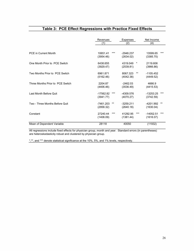
Omitted variable bias is a concern in the previous regressions because of the possibility
of unobserved heterogeneity among physician practices that might be correlated with their
performance on PCE. In the fixed effects model any unobserved time invariant differences across
the PCE practices are captured by the practice-specific intercepts. The results of the estimated
fixed effects model are presented in Table 3. We estimate the same model as before, except we
add practice-level fixed effects and all time-invariant independent variables are omitted from the
regression.
Adding fixed effects increases the magnitude of the coefficient of interest (PCE in
Current Month), but qualitatively does not change our results: switching onto PCE has a positive
effect on profitability, and the effect comes almost entirely from changes in revenues and not
costs. The fixed effects appear to be important, as the magnitude of the PCE effect is
significantly larger than in the OLS regressions. The practices that switched onto PCE
experienced an increase of roughly $10,600 per doctor in monthly revenues. Average revenues
per doctor for the PCE practices during their time on salary was roughly $33,000, so this suggests
an increase of roughly 32% in revenues as a result of the transition onto PCE.7 Given that the
PCE effect on revenue is so large, and that the PCE effect on costs is negative (though not
significant), it is not surprising that we find a large positive effect of PCE on net income. The
physicians who switched onto PCE earned an extra $14,000 per doctor in profits each month
while on PCE. Again, the magnitude of this effect in the fixed-effects model suggests that the
omitted variable bias in the standard OLS estimation was lowering the estimated PCE effect
substantially.
7 Recall that this transition occurs over a period of time where the prices received per procedure are constant, so the changes in revenue must have been generated through changes in quantities.

17
The magnitude of the PCE effects on revenues and net income are large and are not
simply a function of the business getting better with time. While it is true that the bulk of the
PCE months occur late in the sample, the time trend captures any increase through time that is
common to all practices. To further investigate any time pattern in the PCE effect, we estimated
an additional fixed effects model and interacted the PCE effect with a time variable equal to the
number of months since the practice converted to PCE. These results are presented in Table 4.
The results on revenues in column 1 suggest that there is an upward shift in revenues (of roughly
$2400) associated with the move to PCE – although that level effect is no longer significant at
standard confidence levels – and that doctors on PCE increase their revenues by $2150 each
month (p<0.01). Obviously we would not expect this trend to continue indefinitely; the data we
have examined suggest that the incentive effects from the PCE program have not yet plateaued.
Neither PCE coefficients are significant in the cost regression presented in column 2, though the
stationary effect of PCE (the coefficient on PCE in current month) is roughly 10 times larger than
the time trend on the PCE effect. Finally, the stationary effect of PCE on net income is large and
significant (p<0.10), and about five times larger than the time trend component of the PCE effect.
The net income results suggest a one-time gain in profitability of $7,700 (p<0.10) followed by an
increase of an additional $1500 each month (p<0.10). This final set of results suggests that the
effect of PCE on productivity grew over time. As with revenues, we expect that with a longer
time series of post-PCE data we would detect a leveling off of the PCE effect.
Conclusions
We find empirical evidence to support our three main hypotheses, that the poorly
performing doctors would leave, that more productive doctors would be induced to join, and
those groups placed under PCE would be more profitable. Increased revenues and not decreased
costs were the primary source of financial gain for the practices placed under PCE. This occurred
at a time when the underlying prices for the services provided were roughly constant, so the
18
significant increase in revenues must have come from an increased quantity of services provided
(the extensive margin) or a reshuffling of services provided towards more highly-reimbursed
activities (the intensive margin).
Unfortunately, we were unable to obtain more specific data regarding the activities of the
doctors over this time period to identify the exact source of the increase in revenues, and to more
accurately determine whether this change is beneficial to patients or not. The anecdotal stories
conveyed to us by HCA officials describe doctors that previous worked enough to see 15 patients
a day, and that under PCE the doctors saw 30 patients in a day. A change in effort of this
magnitude, without any other change in the mix of services provided, could plausibly result in the
30% increase in revenues we estimate – or more for some doctors. Again, doctors could achieve
those numbers by seeing each patient for less time per visit. Without the detailed data on
physician activity, it is not possible to reach a definitive conclusion about welfare changes as a
result of this new compensation system. Of particular concern is the effect on quality of care. It
is certainly plausible that physician practice financial performance and quality of patient care are
negatively correlated, at least in the short run. To analyze the complete welfare effects of these
compensation systems, one would have to consider the effects on patient health outcomes.
Also, the results in this paper do not answer the question of whether hospitals gain
financially by owning physician practices. The financial performance of the practice itself, which
we analyze here, is only part of the financial benefit to hospitals. Perhaps the largest gain from
solidifying relationships with doctors in the community is to ensure larger flows of admissions
into the hospitals themselves. Before implementing PCE, many officials at HCA had decided that
purchasing physician practices had proven to be a bad business, and that the company should
divest itself of its practices as quickly as it could. With the current success of PCE, the company
has begun to look seriously at further acquisitions. Some company officials, however, are
skeptical that purchasing practices has any effect on patient flows, both when the practices are
purchased and later when practices are let go. Testing that conjecture will be an important part of

19
answering the broader question of whether hospitals, in general, should seek to expand their firm
boundaries to include physicians.

20
Appendix
Proposition 1: For Ai ∈ (Ao, pr, Ah, pr], k = k0 and b > b0,
ei, pr > ei, sal .
Proof: First note that under salary, every employee generates the same output regardless
of ability.
ei, sal = e0, sal for all i
Under productivity based pay, employees choose ei* by equating marginal benefit with
marginal cost of supplying effort:
Max ei : U = b* ei + k – C(ei) / Ai
Subject to: U (ei; Ai, b, k) > R (Ai)
⇒ ei* is such that b = C’(ei*) / Ai
Every employee is offered the same productivity contract (b0, k0), so that:
b0 = C’(ei*) / Ai = C’(e0*) / A0 Rearranging terms, we see that optimal effort (output) is increasing in ability for all employees who take up the productivity-based contract:
C’(ei*) / C’(e0*) = Ai / A0 > 1 C’(ei*) > C’(e0*) ⇒ ei* > e0* ( because C’’(e)>0 )
Finally, since optimal effort under productivity-based pay is greater than or equal to the effort under salary for the lowest-ability employee (this is implied by the assumption that the firm chooses k = k0 and b > b0), e0* > e0, sal = ei, sal
⇒ ei* > e0* > ei, sal

21
Proposition 2: For the linear piece rate contract (k0, b0), Ah,sal < Ah,pr Proof: Ah,pr is identified by the conditions
G(Ah,pr) - R(Ah,pr) = 0
G’(Ah,pr) - R’(Ah,pr) < 0
Ah,sal cannot be the highest ability worker to accept the piece rate contract (b0, k0) because G(Ah,sal) - R(Ah,pr) > 0. Recall that H(A)=R(A) for Ah,sal , so
G(Ah,sal) - R(Ah,sal)
= G(Ah,sal) - H (Ah,sal)
= b0eh + k0 – C(eh) / Ah - s + C(e0) / Ah Substituting a linear Taylor approximation for C(eh) = b0eh + k0 - s - [C’(e0) (eh – e0)]/ Ah Substituting k0 = s - b0e0 and b0=C’(eh*) /Ah yields: = [C’(eh*)(eh – e0)] / Ah – [C’(e0) (eh – e0)]/ Ah = C’(eh) - C’(e0) > 0
⇒ G(Ah,sal) - R(Ah,sal) > 0 For some Ah,pr > Ah,sal it must be true that: G(Ah,pr) - R(Ah,pr) = 0 b0eh* + k0 – C(eh*) / Ah - R(Ah,pr) = 0 Let R(Ah,pr) = z * Ah,pr. Substituting, b0eh* + k0 – C(eh*) / Ah – z Ah,pr = 0 z = (b0eh* + k0) / Ah – C(eh*) / Ah
2 For Ah,pr to be the highest ability worker to accept the contract, is must be that
G’(Ah,pr) - R’(Ah,pr) < 0 : G’(Ah,pr) - R’(Ah,pr)
= b0(deh*/d Ah) – (C’(eh*) / Ah) (deh*/d Ah) + C(eh*) / Ah2 – z

22
= C(eh*) / Ah
2 – z Substituting the above value for z, G’(Ah,pr) - R’(Ah,pr)
= C(eh*) / Ah2 – (b0eh* + k0) / Ah + C(eh*) / Ah
2 = – (b0eh* + k0) / Ah< 0

23
References Barro, Jason R., Kevin J. Bozic, and Aaron M. G. Zimmerman. "Performance Pay for MGOA
Physicians (A)." Harvard Business School Case Study 904-028. 2003. Gaynor, Martin; Mark V. Pauly. “Compensation and Productive Efficiency in Partnerships:
Evidence from Medical Groups Practice,” Journal of Political Economy, Vol. 93, No. 3. 1990.
Hemenway, David, et al. “Physician’s Responses to Financial Incentives,” The New England
Journal of Medicine. Vol. 322, No. 15. April 12, 1990. Lazaer, Edward, 2000. “Performance Pay and Productivity,” American Economic Review,
Review 90(5): 1346-1361. Robinson, James C. 1999. The Corporate Practice of Medicine, Berkeley: University of
California Press.
24
All Groups Always Quit Salary PCE New
Revenues $28,118 $34,552 $18,831 $28,828 $35,282 $37,755(34,808) (47,271) (16,600) (18,704) (22,357) ($47,138)
Expenses $40,050 $44,570 $35,958 $41,149 $40,626 $42,486(34,549) (47,784) (25,434) (23,897) (20,190) (38,015)
Net Income ($11,932) ($10,018) ($17,128) ($12,321) ($5,344) ($4,732)(22,442) (23,379) (24,151) (18,601) (19,628) (16,012)
Number of Observations 1243 309 520 109 71 234
All Numbers are per doctor , but the observations are monthly, physician practice numbers.Standard deviations are in parentheses.The data are from January 1998 to December 1999.
Salary PCE
Table 1: Summary Statistics

25
Revenues Expenses Net Income(1) (2) (4)
Quit: Always on Salary -16766.35 *** -12074.19 *** -4692.165 ***2352.64 (2412.28) (1540.58)
Newly Hired Group 10198.77 *** 2897.72 7301.051 ***(2558.35) (2623.19) (1675.28)
PCE at Any Point -10506.9 *** -8250.166 ** -2256.735 (3975.36) (4076.12) (2603.18)
PCE in Current Month 8863.232 * 2477.263 6385.969 *(5239.77) (5372.59) (3431.15)
Last Month Before PCE Switch 11207.31 10635.5 571.8087 (11829.37) (12129.22) (7746.21)
Second Month Before 11621.62 14199.53 -2577.914 (11805.89) (12105.14) (7730.84)
Third Month Before 6186.565 3349.264 2837.301 (11772.45) (12070.86) (7708.94)
Last Month Before Quit -17664.02 *** -4962.967 -12701.06 ***(6050.78) (6204.16) (3962.23)
Two - Three Months Before Quit -7761.74 * -4159.844 -3601.896 (4343.67) (4453.77) (2844.36)
Constant 44850.09 *** 52129.27 *** -7279.181 ***(3825.02) (3921.97) (2504.73)
Mean of Dependent Variable 28118 40050 (11932)
All regressions include fixed effects for month and year. Standard errors (in parentheses) are heteroskedasticity robust and clustered by physician group.
*,**, and *** denote statistical significance at the 10%, 5%, and 1% levels, respectively.
Table 2: Selection and Improvement Regressions
26
Revenues Expenses Net Income(1) (2) (4)
PCE in Current Month 10651.41 *** -2948.237 13599.65 ***(3954.46) (2634.02) (3385.70)
One Month Prior to PCE Switch 6438.655 4319.049 * 2119.606 (3929.47) (2539.81) (3966.86)
Two Months Prior to PCE Switch 6961.871 8067.323 ** -1105.452 (5162.46) (4042.38) (4449.52)
Three Months Prior to PCE Switch 2204.87 -2462.03 4666.9 (4406.46) (3536.49) (4415.53)
Last Month Before Quit -17562.82 *** -4309.576 -13253.25 ***(3941.77) (4070.27) (3742.59)
Two - Three Months Before Quit -7461.203 ** -3259.211 -4201.992 **(2958.32) (2640.18) (1630.04)
Constant 27240.44 *** 41292.95 *** -14052.51 ***(1408.09) (1381.44) (1616.07)
Mean of Dependent Variable 28118 40050 (11932)
All regressions include fixed effects for physician group, month and year. Standard errors (in parentheses) are heteroskedasticity robust and clustered by physician group.
*,**, and *** denote statistical significance at the 10%, 5%, and 1% levels, respectively.
Table 3: PCE Effect Regressions with Practice Fixed Effects
27
Revenues Expenses Net Income(1) (2) (4)
PCE in Current Month 2757.085 -4972.812 7729.897 *(3476.87) (3461.35) (3939.65)
Number of Months since PCE Conversion 2149.091 *** 584.5887 1564.502 *(704.99) (544.71) (834.82)
One Month Prior to PCE Switch 6836.327 * 4594.385 * 2241.942 (3901.82) (2613.53) (3915.74)
Two Months Prior to PCE Switch 7398.697 8311.925 ** -913.2283 (5133.64) (4137.94) (4409.02)
Three Months Prior to PCE Switch 2740.547 -2354.484 5095.031 (4371.04) (3596.92) (4322.84)
Last Month Before Quit -17327.82 *** -4286.046 -13041.77 ***(3978.43) (4096.15) (3749.56)
Two - Three Months Before Quit -7311.002 ** -3122.266 -4188.736 ***(2960.84) (2665.99) (1611.10)
Constant 2149.091 *** 584.5887 1564.502 *(704.99) (544.71) (834.82)
Mean of Dependent Variable 28118 40050 (11932)
All regressions include fixed effects for physician group, month and year. Standard errors (in parentheses) are heteroskedasticity robust and clustered by physician group.
*,**, and *** denote statistical significance at the 10%, 5%, and 1% levels, respectively.
Table 4: Dynamic PCE Effect Regressions with Practice Fixed Effects
28
Figure 1
Y
S
K0e0 e
U(s,e;A0) b0

29
Figure 2
Y
S
K0e0 e
slope = b0
e1*
b0e1*-K0
U (s,e0; A0)
U (s,e0; A1)
U (s,e1*; A1)
30
Figure 3
U
R (A)
AAh,sal Ah,pr
G (A)
H (A)
A0

31
Figure 4
U
A0(K1)
G (A;K1)
G (A;K0)
R (A)
A0(K0)
K1 < K0
b = b0
Ah(K0) AAh(K1)

32
Figure 5
U
A0(b0)
G (A;b0)
G (A;b1)
R (A)
A0(b1)b1 > b0
K = K0
Ah(b1) AAh(b0)
33
Figure 6: Trends in Average Monthly Financial Performance of HCA Florida Physician Practices
-$30,000
-$20,000
-$10,000
$0
$10,000
$20,000
$30,000
$40,000
$50,000
$60,000
0 6 12 18 24
Month: January 1998 - December 1999
Dol
lars
per
Doc
tor
Revenues Expenses Net Income
34
Figure 7: Average Revenues for PCE Switchers in the Months Relative to PCE Transition
$10,000
$15,000
$20,000
$25,000
$30,000
$35,000
$40,000
$45,000
$50,000
$55,000
-20 -15 -10 -5 0 5 10
Number of Months Relative to PCE Transition
Rev
enue
s pe
r Phy
sici
an ($
)