Embed Size (px)
Citation preview

NBER WORKING PAPER SERIES
A TEST OF INTERNATIONAL CAPM
Charles Engel
Anthony Rodrigues
Working Paper No. 2054
NATIONAL BUREAU OF ECONOMIC RESEARCH1050 Massachusetts Avenue
Cambridge, MA 02138October 1986
We would like to thank Alberto Giovannini for making his data setavailable to us. We would also like to thank Lawrence Plante forresearch assistance. The research reported here is part of theNBER's research program in International Studies. Any opinionsexpressed are those of the authors and not those of the NationalBureau of Economic Research.

NBER Working Paper #2054October 1986
A Test of International CAPM
ABSTRACT
We propose and implement a Wald test of theinternational capital asset pricing model. Ex post assetreturns are regressed on asset supplies. CAPM reequires thatthe matrix of coefficients from a regression of n rates ofreturn on n asset supply shares be proportional to thecovariance matrix of the residuals from those regressions.We test this restriction in the context of a model thataggregates all outside financial assets for each of tencountries. We do not find strong support for therestrictions of CAPM.
Charles Engel Anthony RodriguesNBER Dept. of Economics1050 Massachusetts Ave. Fordham UniversityCambridge, MA. 02138 Bronx, NY. 10458

1.. Introduction
The capital asset pricing model (CAPM) is a popular description of
investors' behavior, but one which has received mixed support empirically. As
applied to international asset markets, it implies that demand for foreign
bonds depends on real exchange rate risk and real rates of return. In this
paper we propose a simple Wald test of CAP?1, and apply the test to a ten
country asset pricing model.
Our test is closely related to a test of CAPM implemented by Frankel
(1982..1983a,1983b,1984) in several recent papers. Unlike previous tests of the
model, the Frankel procedure allows completely unrestricted movements in
expected returns and in "betas" (the covariance of an asset's rate of return
and the market rate of return). It also formulates a natural alternative
hypothesis to CAPM, thus allowing a statistical test of the restrictions
imposed by CAPM. The technique we employ retains almost all the desirable
properties of the Frankel test but eliminates perhaps its biggest difficulty
-— the fact that if the market consists of n assets, n2 parameters must be
estimated with an extremely complex, nonlinear maximum likelihood procedure.
We replace Frankel's likelihood ratio test with a Wald test. The Wald test
requires estimation without imposing the restrictions of the CAPM model ——
which in this case implies that only least squares regressions are employed.
Because estimation is easier, we can extend the empirical model to include
larger collections of assets.
As a general model, one might estimate a system of equations in which the
expected return of any asset is a linear function of the shares of all assets

-2—
in the market portfolio. CAPM constrains the matrix of coefficients from
these regressions to be proportional to the variance-covariance matrix of the
regression errors of the system. The Wald test looks to see if the matrix of
coefficients that comes from the unconstrained estimation is proportional to
the estimated covariance matrix of the residuals. This procedure requires
only the output from OLS regressions. Furthermore, since there are
closed-form expressions for OLS estimates and for the Wald statistic, our
results are completely reproducible The same cannot be claimed for Frankel's
technique, which employs.a "hill-climbing" method to find the maximum of the
complicated restricted likelihood function. There, the estimated coefficients
will depend on such things as the size of the steps taken in climbing the
hill, and the degree of precision set for the estimates.
We apply the Wald test of CAPM to an international asset pricing model.
There are ten assets which represent aggregate bonds held by the public in ten
currencies of denomination. In some ways this model performs better than
previous smaller-scale models. When we have a priori convictions about the
signs of coefficients they usually turn out to be correct in the estimation.
In a joint test of the significance of all the restrictions of CAPM, we find
we cannot reject the model at the 5 percent level. However, the CAPM
hypothesis imposes a very large number of restrictions, so, given the limited
data set (141 monthly observations), the test seems to have low power. A test
of a subset of the restrictions of the hypothesis strongly rejects the CAPM
model.
Section 2 of this paper reviews the CAPM hypothesis and discusses the
relative merits of the likelihood ratio and the Wald tests. In Section 3, we

—3-
use the Wald method to test international CAPM. First we use the data set of
Frankel and Engel (1984) so that we can directly compare our test to
Frankel's. Then we use the Wald test on a larger model over a longer time
period. The concluding section discusses the limitations of these tests, and
outlines the possibilities for future research. In the Appendix, we present
the formulas for calculating the Wald statistic.
2. Testing CAPM
It is useful in developing our test to review the capital—asset-pricing
model.1 A well-known relation that emerges from CAPH is that for any asset i,
(1) Et(r—r0) = itEt(rmt—rot)
where
r1 = real return on asset i from time t to t+1
r0 = riskiess real rate of return
rmt = real return on the market portfolio.
The coefficient it is, in general, a time-varying coefficient that is defined
as
(2) it = Covt(r1, rmt)/Vart(rmt).
Using equation (2), we could rewrite (1) as the "security market line"
(3) Et(r—r0) = p Covt(r1, rmt)
where

—4-
(4) p = Et(rmt_r0t)/Vart(rmt).
The coefficient p is known in the finance literature as the market price of
risk -- it represents the tradeoff between the expected return on the market
portfolio and the variance of return on that set of assets. A critical
assumption is that this "price" is constant over time. In a representative
investor model, this variable can be shown to be equal to the investor's
coefficient of relative risk aversion, which might plausibly be constant. In
reality, the variable could change over time if investors do not have constant
relative risk aversion, or if there are significant income redistribution
effects. However, the assumption of constancy of p seems quite innocuous
compared to some other common assumptions made to test CAPM (see Frankel
(1982,1984) for a discussion of these).
Since there is no asset that is riskless in real terms, to implement (3)
empirically, it is useful to rewrite expected returns relative to the return
on asset 1:
(5)E(r—rit) = p Cov(r—rit, rmt)
= p Cov(r—r1, r1) + p Cov(r1—rit, rmt—rlt).
The return on the market portfolio is a weighted average of returns on each of
the individual assets:
n
r = ZA.r.mt
j=1jt jt
where
= ratio of the value of outstanding shares of asset j to the

—5—
value of all assets.
Therefore, we can write
Covt(r1t_r1, rmt_rit) =
(6)
r_r1).
One can see that Covt(r.-ri, rmt_r1t) could vary over time either because
supplies of assets (the As) change, or because the underlying stochastic
process of returns is time-varying, meaning that Cov(r1t, r) is not
constant. We assume only the As move over time.
Let z. r. - r1. and then use (6) to recast (5) as
(7) Etz.t = Cov(z., ri) + p ZX.Cov(z., zt).
In matrix form we have
(8) Etzt = p Cov(zt, r1) +
where
z vector of asset returns relative to asset 1, j=2,...n
= vector of asset shares, j=2,...n
= Et(zt—Etzt)(zt—Etzt)'.If expectations are rational
z = Etzt +
where is a vector of forecast errors. So, (8) may be written as a system
of regression equations

-6-
(9) z, = c + BAt +
Equation (9) could be a general equation that says the return on an asset
is related to the supplies of all assets in a linear way. Note, however, that
the variance-covariance matrix of is Q. Therefore, the restriction that
CAPM places on the general system (9) is that the matrix of regression
coefficients B be proportional to the covariance matrix of the residuals.
Frankel's method of testing CAPM is to compare the likelihood of the system (9)
without imposing any restrictions on B to the likelihood obtained from
estimating (9) under the restriction that B be proportional to 7. The
likelihood ratio test will fail to reject CAPM if the estimated likelihood with
the restriction imposed is not significantly smaller than the likelihood from
the unrestricted regressions.
The effect on the expected return of asset i (relative to asset 1) of an
increase in the share of asset j is given by the coefficient b3. The CAPM
hypothesis is that this multiplier is proportional to the covariance of the
return on asset i to the return on asset j (each expressed relative to the
return on asset 1), with the constant of proportionality being the market price
of risk. That is,2
(10) = p , V i , j
where
b1 =,th element of B
=..th element of Q.
Since the unconstrained estimation of (9) provides estimates of B and Q, by

—7—
taking the ratios of corresponding elements of the matrices we obtain
(n-i)2 separate estimates of p. We can then construct a Wald statistic that
tests the proposition that all of the ratios are equal.
The Wald-test is equivalent (to the first order) to the likelihood-ratio
test in large samples, but does not require calculation of the restricted
estimates. Estimation of (9) unrestricted requires only n-i ordinary least
squares regressions, each with n-I. right-hand-size variables. Calculation of
the Wald statistic, which is discussed in the Appendix, requires some
relatively simple matrix manipulations involving the data and the estimated
residuals from the regressions. The price for this increased simplicity is
that, if the null hypothesis is true, the unconstrained estimates of B are
less efficient than the estimates of B with the constraint imposed.
3. Testing International CAPM
A hypothesis of considerable interest in international finance is that
international investors are risk neutral and have rational expectations. If
this hypothesis were true, speculators would drive the expected real returns
on all assets into equality (see Engel (1984)). If anticipated real returns
differ among assets, there may be a lack of efficient speculation, but there
may alternatively be a risk premium separating their returns.
The capital asset pricing model outlined in Section 2 provides a
framework for assessing the possibility of risk premia driving a wedge between
anticipated real returns on assets from different countries. This section
takes the approach of aggregating the obligations of each of the countries

-8-
included in the study and considering the real returns on those assets. If
the expected interest rates do differ on these assets, a risk premium is a
likely suspect if the restrictions of the CAPM model cannot be rejected.
Otherwise, we might need to explore the possibility that expectations are not
rational or that asset markets are not fully efficient.
We wish to have as our measure of asset supplies the amount of debt held
by the public denominated in each currency. The measured asset stocks for
each country are essentially the cumulated value of that country's government
deficits. We must correct this figure, however, to allow for foreign exchange
intervention by the country's central bank, intervention into that country's
currency by other central banks, and debt originally issued in foreign
currencies.
The real returns for each asset are calculated as [(1+i)(1+d)/(1+jr)1-1,
where I is the interest rate, d is the rate of depreciation of the currency
relative to the dollar, and ii is a dollar inflation index, it is calculated as
a weighted average of inflation rates of CPIs in all the countries (converted
into dollars) with the weights equalling GNP shares.
The first set of regressions uses the data for six countries that were
used by Frankel and Engel (1984). That data set includes asset supplies for
the U.S., Germany, Japan, Canada, France and England from June 1973 to August
1980. The interest rate used in calculating real returns is the return on one
month Eurocurrency assets.
Table 1 reports the OLS regressions that correspond to equation (9). In
these regressions, dollars are taken as the numeraire asset. A cursory glance
at these estimates suggest that the relation between asset supplies and

-9—
returns -is weak. Few of the coeff-ic-ients are significantly different from
zero. Furthermore, four of the five diagonal coefficients, which we expect to
be positive, are negative. The only positive diagonal coefficient -- for the
yen -- is not significant.
Even though the unrestricted model does not fit the data well, -it is
still possible that we could be unable to reject the restriction that all p's
are equal. Table 2 presents estimates of the covariance matrix 2. A quick
check reveals that there are, ir fact, wide variations in the b../w... Again,
this does not necessarily invalidate the restriction because the coefficients
could be estimated with a low degree of precision.
The Wald statistic for the test that all p's are equal is x2(24)=45.36.
This rejects the null hypothesis at the 1 percent level.
The estimated p's are not very close to 2, so, not surprisingly, the test
of the hypothesis that all the p's are equal to 2 can easily be rejected at
the 1 percent level. The statistic in this case is X2(25)=45.45. This
corresponds to the test in Frankel and Engel. They also reject the null
hypothesis and report a likelihood ratio test statistic of 2(25)59.O. Thus,
even with a limited number of observations the Wald statistic and the LR
statistic are quite close.
The next set of regressions uses asset supplies and returns -From ten
countries from April 1973 to December 1984. This collection includes the
original six countries plus Belgium, Italy, the Netherlands and Switzerland.
The asset supply data comes from Giavazzi and Giovannini (1986). The interest
rates are government bond yields which, along with the exchange rate and price
data, are collected from International Financial Statistics.

-10-
The regressions corresponding to equation (9) are reported in Table 3,
and Table 4 contains estimates of 2. We tested each by equation for
autocorrelation of the error terms using the Breusch (1978) and Godfrey (1978)
test, allowing for serial correlation up to a twelfth order AR or MA process.
Only in the case of the Canadian regression did we find even remote evidence
of correlated residuals, so we made no corrections for this problem.
We also tested for heteroskedasticity using the White (1980) test. Here
we did find evidence of a problem -- five of the tests were significant at the
5 percent level. However, no statistic was significant at the 1 percent
level. A general correction for heteroskedasticity in this model might be
quite difficult because, under the null hypothesis, the coefficient matrix
would vary over time if the variance matrix did. OLS regressions do not yield
consistent estimates of the residuals. Given the somewhat weak evidence for
heteroskedasticity, we attempt no correction, while recognizing this may
render our test statistics inconsistent.
The results reported in Table 3 are somewhat more encouraging than those
from the smaller model. Six of the nine diagonal elements have the postulated
positive sign. None of the three that are negative is significantly different
from zero. Moreover, we cannot reject the restrictions of the CAPM
hypothesis. The statistic for equality of all the p's is x2(80)=100.98. The
statistic for the test that all the p's are 2 is x2(81)=1O1.04. Neither can
reject at the 5 percent level of significance. This is the opposite
conclusions from the one reached using only six assets.
There is, however, evidence that the test has low power. We are testing
a very large number of restrictions. Tables 3 and 4 reveal that the point

—11—
estimates of the p's vary greatly. We must conclude that they are est-imated
with low precision. For example, we are also unable to reject (at the 5
percent level) the hypothesis that all p's are zero. This would imply that
the risk-neutral uncovered interest parity formulation holds.
One way to increase the power of the test is to test only a subset of the
restrictions. When we test for equality only of the diagonal p's, we test
only eight restrictions. This hypothesis is easily rejected at the 1 percent
level.
4. Conclusion
The evidence presented in Section 3 does not provide strong support f or
international CAPM. However, it does apply a methodology that might be useful
in future work in this area. There are still several weaknesses of tests of
this nature, several of which are discussed by Frankel and Engel. In our
conclusion, we will concentrate on a problem that they did not discuss in
great detail.
This type of test of CAPM requires that the vector of asset shares
contain correctly measured shares of all assets available to investors.
Aggregation of assets is only strictly correct if the assets lumped together
are perfect substitutes -in investors' portfolios. There are several reasons
why the data set used here, though very carefully constructed, may fall short
of the ideal.
To begin with, the aggregation of all obligations of a government into a
single asset is clearly inappropriate. For example, long-term bonds and

—12—
short-term bonds certainly have different risk characteristics.
The vector of assets described here contains no measure of real assets.
For example, Frankel (1984) uses measures of the value of the housing stock
and other tangible assets, and the value of corporate equities in his study
using U.S. data. This, too, suffers from too much aggregation. All stocks
are collected together as a single asset, when, in fact, CAPM was originally
formulated as an explanation of how risk and return characteristics of stocks
differ.
Clearly, a good test of an international version of CAPM will require
many right-hand-side variables. We have claimed as an advantage for the Wald
test the simplicity of its estimation technique and the ease with which
results can be reproduced. We also believe that it has a large advantage in
terms of the size of the model that can be handled. There are some problems
of dimensionality with the Wald test. It requires, if there are n assets,
estimation of n-i regressions, each with n-i regressands. Furthermore, the
calculation of the Wald statistic requires inversion of a matrix with (n-1)2-i
rows and columns. Although these might require a large amount of calculation,
there are very efficient programs written for OLS estimation and matrix
inversion. On the other hand, the constrained likelihood estimation could be
very time consuming and expensive. At each iteration on the parameter
estimation a n(n-i)/2 x n(n-i)/2 matrix must be inverted (as opposed to a
one-time inversion of a slightly larger matrix in calculating the Wald
statistic). If n is very large, the maximization routine may require many
iterations to achieve convergence. Furthermore, the matrix inversion
technique imbedded in most maximization routines is unlikely to be as

—13-
efficient as one that can be called separately for the one-time inversion
required for the Wald statistic.
We believe there is still promise in testing international CAPM. Much
work is left to be done in assembling good data sets. The principle of the
Frankel technique seems correct, but, because of dimensionality problems, and
the difficulty of estimating the constrained likelihood function, there does
not seem to be much hope of applying his method directly to large systems.
The Wald test, though, offers a more feasible alternative.

—14-
Appendix
The Wald Statistic3
If 0 is a vector of parameters, and we wish to test the hypotheses
h(9) = 0 i=i,...,p
the Wald statistic provides a test of the closeness to zero of the vector
h(0) = (h1(0), h2(0) ... h(0))'where the represents the estimated values of parameters.
If there are s parameters, let H.. be the sxp matrix9
H.. (ah.(o)/ao.].0 3 1
Furthermore, let B represent the estimated information matrix of the0
parameters. Then, if there are T observations, the Wald statistic, given by
= T(h(0)]'(H'B:1H]1[h(9)],009is asymptotically distributed x2(r).
In our case, we want to test the hypothesis that the are equal
for all I and j. If there are n assets, there are n—i regressions, and
(n-i)2 coefficients in the B matrix. This implies that there are (n-1)2—1
independent constraints to be tested. There are many different ways to write
these constraints (for example b11/c11 = b12/,i12, b12/w12 = b13/w13, etc., or
b12/w12 = b11/11, b13/w13 = b11/w11, etc.) but the calculated value of the
Wald statistic, in this instance, is independent of the way the constraint is
written. We choose to express the constraints relative to the last element --
that is,
b1/w1 - bn...i,n_i/Wn...i,n...i= 0.
In the tests we report in Section 3, the elements in our h(6) are obtained by

—15—
reading across B in rows —— (with n=6) the first element is b11/w11 - b55/w55,then b12/w12 - b55/co55, b13/w13 - b55/55 ... b54/w54
-b55/w55.
Each row of H.. contains the derivative of every constraint with respect
to one parameter. The first (n-i)2 rows of H contain the derivatives of
constraints with respect to the elements of the B matrix. Again, the
parameters are taken from B row by row. There are only n(n—1)/2 independent
parameters in Q. The next n(n-1)/2 rows of H.. are comprised of the0
derivatives of the constraints with respect to the elements of Q. If is
expressed in lower triangular form, the elements of Q are taken row by row
(i.e., with n=6, WU, 21 22 w55). It is useful to write the
matrix H as
H =
[ : Iwhere H1 is (n—i)2 x E(n—1)2—i] and H2 is [n(n—1)/2) x [(n—i)2—l).
The inverse of the information matrix is given by
B1— 11—0
V22
In this matrix, if E is the estimated covariance matrix of the right-hand-side
variables, then
Vii = x
The matrix V22 is the covar-iance matrix of the estimates of . The element
corresponding to the covariance of Wpq and rs is given by WprWqs +ps"qr(see Rothenberg (1973), pp. 87—88).
From above, the expression for the Wald statistic can be rewritten as
T(h(9)]'[HV11H1 + HV22H2][h(e)].Notice that the statistic requires only the estimated coefficients, the
covariance matrix of the residuals, and the covariance matrix of the asset
—16-
shares. All calculations for the test statistic, as well as for the
estimation, involve only simple linear algebra.
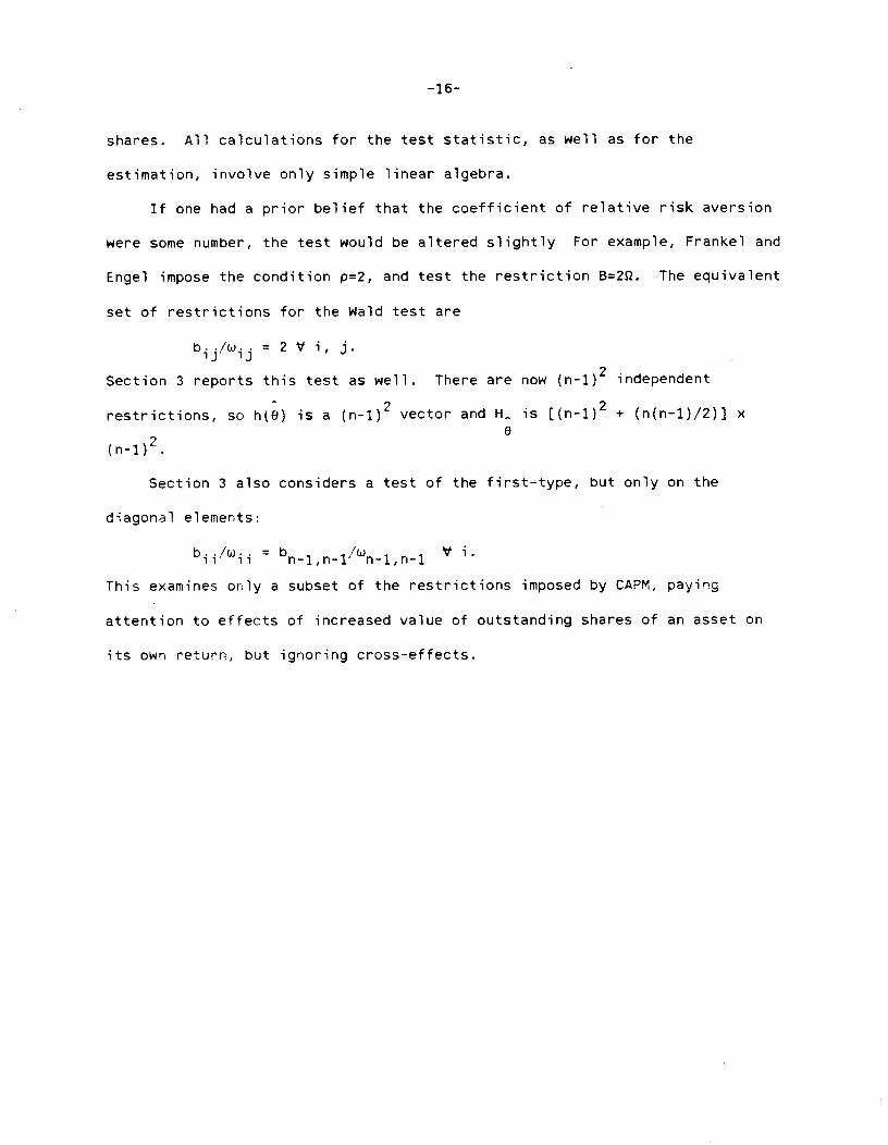
If one had a prior belief that the coefficient of relative risk aversion
were some number, the test would be altered slightly For example, Frankel and
Engel impose the condition p=2, and test the restriction B=2I. The equivalent
set of restrictions for the Wald test are
= 2 V i, j.
Section 3 reports this test as well. There are now (n-i)2 independent
restrictions, so h(D) is a (n-i)2 vector and H. is [(n-i)2 + (n(n-1)/2)] x0
()2Section 3 also considers a test of the first—type, but only on the
diagonal elements:
b/w1 = bn_i,n_i/Wn_i,n_i V i.
This examines oily a subset of the restrictions imposed by CAPM, paying
attention to effects of increased value of outstanding shares of an asset on
its own return, but ignoring cross-effects.

—17—
Foot notes
1. This discussion draws on Frankel's (1983b) presentation of his CAPM test.
2. There is a possibility that = 0, i j, so that the ratio b1/w is
undefined. Under most plausible assumptions of the underlying forces that
determine the forecast errors, this would be an event with probability zero.
Nonetheless, this may be a justification for testing equality only of the
ratio of the diagonal elements, as is done in Section 3. One might consider
writing the constraints in such a way as to avoid possible division by zero,
such as b11w12 = b12w11, b12w13 = b13w12, etc. However, unlike the test for
equality of the p's. the calculated test statistic will depend on the way the
constraints are written. The statistic for the test b11w12 =b12w11, b12w13 =
b13w12, etc. will not be the same as the one for b11w12 = b1211, b11w13 =
b13w11, etc.
3. The discussion of the Wald test draws on Silvey (1975).
4. See footnote 2 for further discussion.

—18-
References
Breusch, 1. 1978. "Testing for Autocorrelation in Dynamic Linear Models,"
Australian Economic Papers 17: 334-55.
Engel, C. 1984. "Testing for the Absence of Expected Real Profits from
Forward Market Speculation," Journal of International Economics 17:
299-308.
Frankel, J. 1982. "In Search of the Exchange Rate Premium: A Six-Currency
Test Assuming Mean-Variance Optimization," Journal of International
Money and Finance 1: 255—74.
__________ 1983a. "Estimation of Portfolio—Balance Functions that are
Mean-Variance Optimizing: The Mark and the Dollar," European Economic
Review 23: 315—27.
_________ 1983b. "Portfolio Shares as 'Beta—Breakers': A Test of CAPM,"
Journal of Portfolio Management, forthcoming.
__________ 1984. "Portfolio Crowding Out Empirically Estimated," Quarterly
Journal of Economics, forthcoming.
_________ and C. Engel. 1984. "Do Asset Demand Functions Optimize Over the
Mean and Variance of Real Returns? A Six-Currency Test," Journal of
International Economics 17: 309-23.
Giavazzi, F. and A. Giovannini. 1986. "European Currency Experience,"
Economic Policy 1, forthcoming.
Godfrey, L. 1978. "Testing Against General Autoregressive and Moving Average
Error Models When the Regressors Include Lagged Dependent Variables,"
Econometrica 46: 1293-1302.

—19—
T. 1973. Efficient Estimation With A Priori Information. New
Conn.:
1975. ______________________
1980.
Direct
Yale.
Statistical Inference. New York, NY: Wiley.
"A Heteroskedasticity-Consistent Covariance Matrix Estimator
Test for Heteroskedasticity," Econometr-ica 48: 817-38.
Rot henberg,
Haven,
Silvey, S.
White, H.
and a
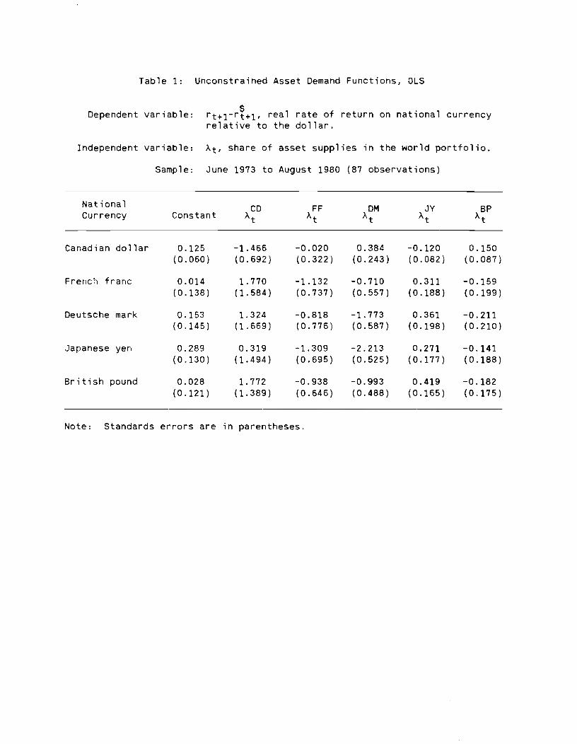
Table 1: Unconstrained Asset Demand Functions, OLS
Dependent variable: rt+l-r+1, real rate of return on national currencyrelative to the dollar.
Independent variable: Xt, share of asset supplies in the world portfolio.
Sample: June 1973 to August 1950 (57 observations)
National
Currency ConstantCDX
FFX
DM JY BP
Canadian dollar 0.125
(0.060)
-1.466(0.692)
-0.020
(0.322)
0.384
(0.243)
-0.120
(0.082)
0.150
(0.087)
French franc 0.014
(0.138)
1.770
(1.584)
—1.132(0.737)
—0.710(0.557)
0.311
(0.188)
—0.159(0.199)
Deutsche mark 0.153
(0.145)
1.324
(1.669)
-0.818(0.776)
-1.773
(0.587)
0.361
(0.198)
—0.211(0.210)
Japanese yen 0.289
(0.130)
0.319
(1.494)
-1.309(0.695)
-2.213
(0.525)
0.271
(0.177)
—0.141(0.188)
British pound 0.028
(0.121)
1.772
(1.389)
-0.938
(0.646)
-0.993
(0.488)
0.419
(0.165)
—0.182(0.175)
Note: Standards errors are in parentheses.

Table 2: Variance-Covariance Matrix of Residuals
(from regressions reported in Table 1)
w1,CD FF DM JY BP
Canadian dollar .1686x103
French franc .6552x104 .8825x104
Deutsche mark .9881x104 .7777x103 .9804x103
Japanese yen —.6849x103 .4156x103 .3699x103 .7848x103
British pound—
.6004x10.-.
.4261x10—
.4387x10—
.3119x10 .6791x10—,

Table 3
:
Dependent v
ar
able
Unconstrained Asset Demand Functions, OLS
rt+l-r+l, r
eal rate of return on national currency
relative to the dollar.
Note:
Standards errors are in parentheses.
Sample:
April 1973 to December 1984 (141 observations)
National
BE
Currency
Constant
At
CD
At
FF
At
DM
At
IL
At
JY
At
DG
Xt
SF
At
BP
xt
Belgian franc
0.06
(0.14)
2.42
(1.69)
-2.74
(1.54)
—0.18
(0.78)
-1.61
(0.64)
-0.54
(0.42)
-0.20
(0.23)
8.51
(2.97)
1.94
(2.12)
0.09
(0.22)
Canadian dollar
-0.13
(0.06)
-0.71
(0.68)
1.09
(0.62)
0.34
(0.32)
0.27
(0.26)
—0.11
(0.17)
0.25
(0.10)
2.40
(1.20)
—0.85
(0.85)
-0.09
(0.09)
French franc
0.12
(0.14)
1.78
(1.68)
—2.44
(1.52)
-0.12
(0.77)
—1.37
(0.63)
-0.57
(0.42)
-0.19
(0.24)
5.27
(2.95)
1.59
(2.10)
0.17
(0.26)
Deutsche mark
0.07
(0.14)
2.53
(1.71)
-2.83
(1.55)
-0.49
(0.78)
-1.21
(0.65)
-0.48
(0.43)
-0.29
(0.24)
8.01
(3.00)
1.01
(2.14)
0.01
(0.22)
Italian lira
0.20
(0.12)
2.64
(1.47)
-2.35
(1.33)
-0.09
(0.67)
-1.56
(0.55)
—0.55
(0.37)
—0.33
(0.21)
1.87
(2.58)
3.07
(1.84)
0.29
(0.20)
Japanese yen
0.01
(0.14)
-0.86
(1.67)
-0.14
(1.52)
-0.36
(0.77)
-0.75
(0.63)
0.06
(0.42)
0.08
(0.24)
-0.60
(2.94)
3.44
(2.09)
0.24
(0.22)
Dutch guilder
0.10
(0.14)
2.54
(1.65)
-3.18
(1.50)
-0.39
(0.76)
-1.45
(0.62)
-0.66
(0.41)
-0.28
(0.23)
8.65
(2.90)
1.55
(2.07)
0.66
(0.22)
Swiss franc
0.19
(0.15>
3.76
(1.86)
-3.82
(1.69)
-0.79
(0.85)
—2.26
(0.70)
-0.41
(0.47)
-0.56
(0.26)
6.77
(3.27)
6.07
(2.33)
-0.04
(0.25)
British pound
0.19
(0.12)
1.88
(1.50)
-1.88
(1.36)
-0.36
(0.69)
-1.04
(0.57)
-0.86
(0.37)
-0.25
(0.21)
2.64
(2.63)
0.64
(1.87)
0.33
(0.20)

Table 4: Variance-Covariance Matrix of Residuals
(from regressions reported in Table 1)
National
Currency BF CD FF DM IL JY DO SF BP
Belgian franc .975
Canadian dollar .118 .157
French franc .827 .100 .957
Deutsche mark .932 .101 .831 .993
Italian lira .579 .072 .633 .592 .731
Japanese yen .537 .065 .548 .543 .411 .949
Dutch guilder .896 .107 .803 .916 .587 .527 .927
Swiss franc .859 .117 .805 .908 .592 .611 .853 1.174
British pound .491 .095 .456 .471 .364 .413 .487 .482 .760
Note: All numbers have been multiplied by 1000.