afIC FILE CQO (I

NAVAL POSTGRADUATE SCHOOLMonterey, California

%o TRAD

THESIS

THE ;NALYSIS OF THERMAL RESIDUAL STRESS FORMETAL MATRIX COMPOSITE WITH

Al/SiC PARTICLES

byHur, Soon Hae

June 1988

,%

',Thesis Advisor: Chu Hwa. Lee

SiApproved for puihic release: distribution is unlimited

DTICNOV 0 11988

V *E

jc"

-jD

Unc assi eERITY CLAS5FICATION OF THIS PAGE

REPORT DOCUMENTATION PAGEIa. REPORT SECURITY CLASSIFICATION lb RESTRICTIVE MARKINGS

1lt] i figid

2a. SECURITY CLASSIFICATION AUTHORITY 3 DISTRIBUTION /AVAILABILITY OF REPORT

2b. DECLASSIFICATION /DOWNGRADING SCHEDULE Approved for public release;distribution is unlimited

4. PERFORMING ORGANIZATION REPORT NUMBER(S) S MONITORING ORGANIZATION REPORT NUMBER(S)

6a. NAME OF PERFORMING ORGANIZATION 6b OFFICE SYMBOL 7a NAME OF MONITORING ORGANIZATION(if applicable)

Naval Postgraduate School 61 Naval Postgraduate School

16c. ADDRESS (City, State, and ZIP Code) 7b. ADDRESS (City, State, and ZIP Code)

Monterey, California 93943-5000 Monterey, California 93943-5000

Ba. NAME OF FUNDING ISPONSORING 8b OFFICE SYMBOL 9. PROCUREMENT INSTRUMENT IDENTIFICATION NUMBERORGANIZATION (If applicable)

kc. ADDRESS (City, State, and ZIP Code) 10. SOURCE OF FUNDING NUMBERS

PROGRAM PROJECT TASK WORK UNITELEMENT NO NO NO ACCESSION NO.

11. TITLE (Include Security Classification)

lhe analysis of thermal residual stress for Metal Matrix Composite with Al/SiC particle

12. PERSONAL AUTHOR(S)

13a. TYPE OF REPORT 13b TIME COVERED 14 DATE OF REPORT (YearMonth, Day) 1S PAGE COUNTMaster's thesis FROM TO 1988 June 55

16. SUPPLEMENTARY NOTATION The views ex ressed in this those te athoxand do not reflect tne orrical policy or poslilon ne epar men o De enseor the U.S. Goverment.17. COSATI CODES 18 SUBJECT TERMS (Continue on reverse if necessary and identify by block number)

FIELD I GROUP SUB-GROUP fJherma residual stress, aspet4 .

(Continue Creeping behavior,-r- Volume fraction - --2,-19. ABSTRACT (Continue on reverse if necessary and identify by block number)

When a metal matrix composite is cooled down to room temperature from the fabricationor annealing temperature, residual stresses are induced in the composite due to themismatch of the thermal expansion coefficients between the matrix and fiber. A methodcan be derived for calculating the particles due to differences in thermal expansioncoefficients. Special attention is paid to creep deformation in the matrix phase. The

* analysis shows that considerable internal stresses and creep deformation appear in thecomposites when subjected to cooling. , ,

4

20 DISTRIBUTION/AVAILABILITY OF ABSTRACT 21 ABSTRACT SECURITY CLASSIFlCATION

OUNCLASSIFIEDUNLIMITED 0 SAME AS RPT 0 DTIC USERS Unclassi fied22a NAME OF RESPONSIBLE INDIVIDUAL 22b TELEPHONE (Include Area Code) j 22c OFFICE SYMBOL

Professor Chu Hwa. Lee _(408) 646 - 3036 I 62LeDD FORM 1473. 84 MAR 83 APR edition may be used until exhausted SECURITY CLASSIFICATION OF THIS PAGE

All other editions are obsolete 0 U.S. Government fintlin Office: 1,#4-406-243

Ii

Approved for public release; distribution is unlimited.

The Analysis of Thermal Residual Stressfor Metal Matrix Composite with Al/SiC Particles

by

Hur, Soon HaeLieutenant Colonel, Republic of Korea Army

B.S., Republic of Korea Military Academy, 1975

Submitted in partial fulfillment of therequirements for the degree of

MASTER OF SCIENCE IN ENGINEERING SCIENCE

from the

NAVAL POSTGRADUATE SCHOOLJune 1988

Author: 34Hur, Soon Hae

Approved by: (/ / 41 oV /Chu Hwa. ee, Thesis Advisor

1 y XR. McNelly, Second Reader U"

-Anthon4 / J. Healey, Chairmtn,Department of/.Meehanical Eng eering

Gordon E. Schacher,Dean of Science and Engineering

ii

4 W,

II

II

• rI ~\ ~ -

ABSTRACT

When a metal matrix composite is cooled down to room temperature

from the fabrication or annealing temperature, residual stresses are induced in

the composite due to the mismatch of the thermal expansinn coefficients

between the matrix and fiber. A method can be derived for calculating the

internal stresses appearing in Metal Matrix composites of Al matrix with SiC

particles due to differences in thermal expansion coefficients. Special attention

is paid to creep deformation in the matrix phase. The analysis shows that

considerable internal stresses and creep deformation appear in the composites

when subjected to cooling.

Accession For

NTjIS CRA&IDTIC TAB

!"PY

Unannounced II cJustifftcatio '

By h

Distribution/ -_

AvallabIlity CodesAvift an-d/or

Dist Special

,,

TABLE OF CONTENTS

I. INTRO DU CTIO N ............................................ 1

A. METAL MATRIX COMPOSITES(MMCs) ...................... 1

B. THE ANALYSIS OF MMCs(AI/SiCs)

IN THE STABLE MEMBER ................................. 1

C . PU RP O SE ................................................. 2

II. LITERATUTRE REVIEW ........................................ 3

A . M M C s ................................................... 3

B. ELASTIC MATRIX AND ELASTIC' INCLUSION ............. 3

C. ELASTOPLASTIC MATRIX AND ELASTIC INCLUSIONS- 6

D . C R EEP ................................................... 6

III. THEORETICAL BACKGROUND AND DERIVATION .......... 11

A. THEORETICAL BACKG ROU ND ......................... 11

1. ELASTIC INCLUSIONS AND MATRIX ............. 1)

2. ELASTOPLASTIC MATRIX AND ELASTIC INCLUSIONS.. 12

3. C R E E P) ............................................ 13

B. DERIVATION .......................................... 13

1. ELASTIC INCLUSIONS AND ELASTIC MATRIX ........... 13

2. ELASTOPLASTIC MATRIX AND ELASTIC INCLUSIONS. 16

3. CRE EP ............................................ 20

IV. RESULTS AND CONCLUSIONS ............................. 22

A .R ESULTS ................................................. 22

B. CONCLUSIONS AND RECOMMENDATIONS ..................9

APPENDIX A: PROGRAM FOR VALUE OF Siikl(a'=l.5-,5) .............. 31

iv

APPENDIX B: PROGRAM FOR VALUE OF Sijkl(1=.0.) ............ 3

APPENDIX C: PROGRAM FOR VALUE OF THERMAL RESIDUAL

STRESS, E, ET E- u. and < r >. m ............... 35i1 1] ) 1 ] ii

APPENDIX D: FOPRAIULA OF Sijki FOR A VARIETY OF INCLUSION... 39

APPENDIX E: PROGRAM FOR CREEP DEFORMATION ............... 42

LIST OF REFERENCES ................................................. .

INITIAL DISTRIBUTION LIST .......................................... 45

0v'

%.-4JC..,

LIST OF FIGURES

FIG. 2.1 Variation of creep and creep rate with time .......... 9

FIG. 2.2 Creep rate vs Time ................................. 10

FIG. 2.3 Typical creep curve .................................. 10

FIG. 3.1 Theoretical model................................... 11

FIG. 3.2 Microcreep as a function of time t ...................... 21

FIG. 4.1 internal stress vs aspect ratio ....................

FIG. 4.2 Internal stress vs temperature change(,T)...........

FIG. 4.3 Internal stress vs volume fraction(f)...............

LIST OF TABLES

TABLE 1 The value of E P a=-l, 1. ).......................... 23

TABLE 2 The value of ET( a-1, 1.5 ).........................23

TABLE 3 The value of E<( a=1--, 1.5 .......................... 924

TABLE 4 The value of E ( a l 1.5 ).......................... 24

TABLE 5 The value of cT( a=-1, 1.5 ).......................... 24

TABLE 6 The valae of < (T-I > a=-1, 1.5 ) ..................... 24ij m

TABLE 7 Comparison value of < ( - >, with TAYA'S .............. .27)II0

vii

0%

ACKNOWLEDGEMENTS

I wish to express my gratitude and appreciation to Professor Chu HwaLee and my second reader, Professor Terry . McNelley for the instruction,guidance and advices throughout this research.

Finally, many thanks to my wife, and my son and daughter,

for their love and being healthy and patient for twoand half years

V j

J1ti ~. f * ,fta.~.

I. INTRODUCTION

A. METAL MATRIX COMPOSITES(MMCs)

Discontinuously reinforced Metal Matrix Composites(MMCs) represent a

group of materials that combine the strength and hardness of the reinforcing phase

with the ductility and toughness of the matrix. Aluminum alloys(Al) reinforced

with Silicon Carbide(SiC) in particulate, platelet, or whisker form and fabricated by

powder metallurgy methods are receiving a great deal of attention from researchers

and engineers.

B. TIlE ANALYSIS OF MMC's(AI/SICTs) IN THE STABLE MEMBEFi

Previous research has evaluated the dimensional stability, and the thermal

and mechanical properties of several Al/Si(' MMCs in stablc-member applications

for missile inertial guidance system. The results reveal that, although the candidate

materials from a powder blend of SiC and Al alloy consolidated by Vacuum Hot

Pressing(VHP) into cylindrical billets, followed by Hot Isostatic Pressing(HIP) for

full densification, have better isotropic properties, these MMCs show some micro

creeping behavior in service. The microcreep of these MMCs will affect, the

dimensional stability of stable members, and is likely to arise from two sources: (1)

creep of the metal matrix caused by internal stresses creep conditioned by externally

applied stresses and/or (2) phase transformations during the creep condition. A first

step toward understanding the cause of the dimensional stability problem is to

analyze the influence of internal stresses. The internal stresses are thermal residual

stresses when a Metal Matrix Composite is cooled down to room temperature from

V - I

the fabrication or annealing temperature. Thest residual stresses are indu(,d in the.

composite due to the mismatch of the thermal expansion covfficients ltiwwen th,

aluminum alloy matrix and the silicon carbide particles. The mndt-l. based It

Eshelby's for mismatch problems with simplified linear elastic material behavior for

both particles and matrix, has been used to solve the problem of thermal residu--l

stress [ref 1].

C. PURPOSE

The purpose of this thesis is to calculate the thermal residual stress of Al/SiC"

using theoretical methods and then to determine what influence this thermal

residual stress has on creep deformation. In order to do this. the thermal r-sidualstresses will be determined by focusing on elastoplastic mat rix and elast i inclusiuns

rather than on elastic matrix and elastic inclusions. Therefore, the ca-se where both

phases( matrix and inclusions ) art perfectly elastic will be treated first. Then,. the

theoretical results will be compared with previously obtained experimentai data fr

Al/SiC composites.

2I

I

I4 ;

N N N N % N

FOAO4~ -JW7 -WF ?U-r7, VV. -. . .- . - .1. WrK711 ,

II. LITERATURE REVIEW

A. MM(s

Metal matrix composites(MM(-s), including eutectic compusites, are becoming

important in applications as structural components which are to be at intermediat.

and high temperatures. When MMCs are fabricated at high temperature or annealed

at certain high temperatures, the MMCs have undesirable properties. such as low

tensile yield and ultimate strengths. Those results are mainly due to residual

stresses that are caused by the mismatch of the thermal expansion coefficient

between the matrix and fiber. The residual stresses so induced have been cbstr~ed

in tungsten fiber/copper composites and in SiC whisker/6061 Al comp,,sites and

,',ere based on analyzed a one--dimensional model for a continuous fiber system cr

spherical particle system. The model, based on Eshelby's equivalent inclusion

method, has been used to solvre the problem of thermal residual stressesfref 2].

B. ELASTIC MATRIX AND ELASTIC INC-ULSIONS

Let's consider a two-phase suspension of finite extent in which one phase is a

matrix while the other is in the form of inclusions. It is assumed that the inclusions

can be treated as identical ellipsoids with corresponding axes aligned. Further. the

inclusions are assumed to be randomly distributed in the matrix in such a way that

the suspension is homogeneous on a macroscopic scale. The task of the present

section is to solve Eshelby's transformation problem for the case where the

fractional volume f of the inclusions is finite. Following Eshelby [ref 2], we considerI.

first an auxiliary problem. what is the resulting stress o in an inclusion when everyij

inclusion, having isotropic plastic moduli equal to those of the matrix, is subjected

SM

3t

'€" " " " " 1, •" 4; , .." #. ".€° .-" ,P -"',.' o" ,,¢'.4'"= *.""," d' ,, ." ". " ,,,',, 0

to a uniform transformation strain T, To find the exact solution appears 1n l(

impossible since no detailed information is given about the spatial distribution of

the inclusions. All we may find in this situation ;re approximate average fields. The

average constrained strain E -C in any inclusion may be written in the formti

' =E + E (j

I

Here, E C is the constrained strain in a typical inclusion which would be produced if]j

it alone is embedded in an infinite elastic body. This term is given, according to

Eshelby[ref ]. as

SICT

EC =S ET (2)

3j ijkl i j

Where S is Eshelby's tensor which depends on the aspect ratios of tho ellipsoidalijkl

inclusion and Poisson's ratio.(Here and in the following we use the usual summation

convention: the range of subscripts is form 1 to 3). E"C is a contribution due to allij

the surrounding inclusions and the presence of free boundary; this term is entirelY

elastic, and is assumed to be eiffectivelv constant in and around the typical

(II

inclusion. Then, it will be a good approximation to regard E- as the average

elastic strain in the matrix for the contribution of any one inclusion to the average

field; outside it is negligible when there are a great number of inclusion in the

material. For a homogeneous elastic body in static equilibrium, a volume integral of

any component of the elastic strain associated with an internal stress should vanish

provided that the integration is taken throughout the body. Thus

44

or er,1r~ r F, Ir,, I,

1-0 E-(- + f( - - -T = E E:0

From (1), (2) and (3), we have

E =(1-fS E T + fE T (4)ijkl k I j

The average internal stress in any inclusion is given by

-I =C (- CE T (5)

1) ijkl k I k I

Where (' is the elastic moduli ol the matrix (and also of the inclusions in theij kl ,,

present situation) [ref 3]. Where the inclusions have elastic moduli differing from

those of the matrix, the same approach as used by Eshelby [ref 2] will be applicable.

The essence of this approach is terms of equivalent inclusions. Let (7 be the

elastic moduli of the inclusions, and ET* be a uniform transformation strain of everyI j

inclusion. Then the transformation strain of the equivalent inclusions, E, can beiI-

determined by solving a set of equations

C C(E- T )= ' T* 6Ciil Ekl kl Ejl E

with ( 4 ). The average stress in any inclusion is given by ( 5 ), of course. Consider

a composite specimen which is free of stress at a references temperature To. Let the

matrix and the inclusions have isotropic linear thermal expansion coefficients a and

a respectively. The elastic state when the specimen is subjected to a uniform

%"

%K

temperature change, AT 0=T-TO, is described by the situation where th, matrix

and the inclusions undergo uniform transformation strains oaT, and* i

a &T6 respectively. Here 6 is the Kronecker delta. The resulting state of stress

can be analyzed by putting

ET* (a a) AT (7)lj i3

The overall thermal expansion coefficients a can be expressed as a function of a.

a C , C f and the aspect ratios of the inclusions.ij k1l ij kl

C. ELASTOPLASTIC MATRIX AND ELASTIC INCLUSIONS

When the temperature change is great, one should expect plastic deformation.

either in the matrix and/or in the inclusions, which relaxes the inteinal stress

accumulated. An important practical case, the case where the plastic deformation

occurs only in the matrix, will be considered in the following. Further. for

simplicity, we assume that the plastic strain is uniform throughout the matrix and

the plastically nondeforming inclusions can be treated as identical spheroids. Then,

the plastic strain in the matrix, E.P, may be written in consideration of a symmetric1]

mode of plastic deformation and the volume constant law, as:

E P= E [646 -(6 b6+6)1b(8)jj p 3i 3j h i i 2i 21EP*

Where EP is a temperature-dependent parameter. In this case, the overall strain E j

of the composite is given, with use of Equation T .=fEi.T, byi] I ]

i t w •",

E =aT,+E.P+fET (9)ii I 1 il]

Where E T is calculated from (4) and (6) withIi

E = (a -aTf& -E. ( 10)i j 1) Ij

Now, the temperature dependence of E will be found through an energy-balance

consideration. Since energy dissipative process is involved in plastic deformation,

the decrease in the elastic energy., - 6Eei, corresponding to a virtual plastic

deformation 6EP, should be balanced against the dissipation energy. If the matrix

material has a constant flow stress ay in a uniaxial deformation, the condition is0Y

written as:

-- ,ei = (1-f)oia V iEpI (%>o) (11)

= lfc-1IT*

Where Eel -, 1 ..T- 1) 1

2

,Ep + CE P(a - a)AT

+ C3( a - a)2AT2 (12)

It is noted that when the composite is elastoplatic the following condition should be

satisfied:

(Eel) I > (Eel),,

,,7

Where the subscripts I and 11 refer to the entirely elastic case and the elastopla-stic

case, respectively[ref 31.

D. CREEP

If a stress is suddenly applied to pure metals, some solid solutions and most

engineering alloys at a temperature near or greater than 0.5Tm(where Tm is the

absolute melting point of the metal or alloy) deformation proceeds as shown in Fig.

2.1. The initial application of stress causes an instantaneous elastic strain EO to

occur. If the stress is sufficiently high an initial plastic deformation Ep also occurs.

At low temperatures, significant deformation ceases after the initial applicatin of

stress and an increase in stress is required to cause further deformation. At elevated

temperatures, deformation under a constant applied load continues with time. The

early stage of such deformation called primary creep is characterized by an initially

high creep rate dE/dt which gradually decreases with time. Eventually a linear

variation of creep strain accumulation with time is observed. This steadv--state

creep region is characterized by a constant minimum creep rate. Steady-state creep

rates depend significantly on stress and temperature and are used frequently to

compare the creep resistance among alloys. After significant deformation in

steady-state creep. necking occurs or sufficient internal damage in the form of voids

or cavities accumulate to reduce the cross-sectional area resulting in an increase in

stress and creep rate. The process accelerates rapidly and failure occurs. This region

of the creep curve is called tertiary creep. Fig. 2.1 also shows the derivative of the

creep curve or the creep rate curve. Fig. 2.1 represents the most common creep

strain/time behavior and Fig. 2.2 illustrates the strain rate/time behavior at

temperatures below approximately 0.3Tm. In Fig. 2, only transient creep is

?S

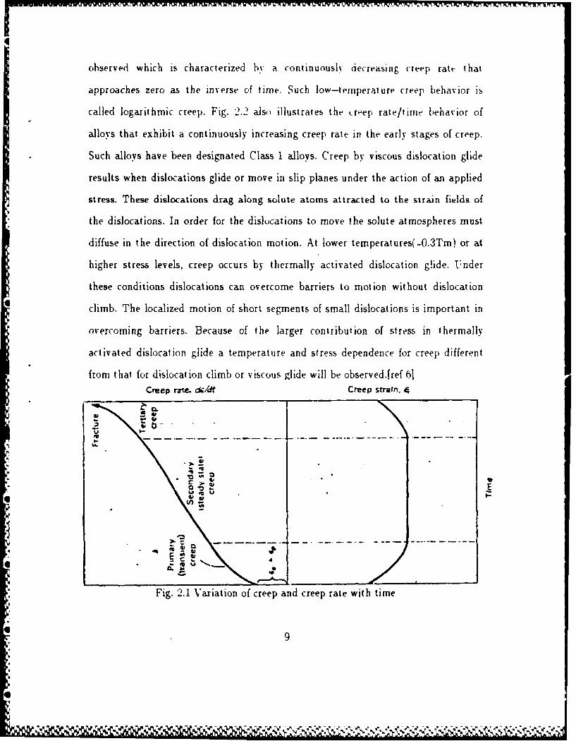
observe.d which is characterized by a continuously decreasing creep ratt- that

approaches zero as the inverse of time. Such low-temperature creep behavior is

called logarithmic creep. Fig. 2.2 als, illustrates the tr,ep rate/time behavior of

alloys that exhibit a continuously increasing creep rate in the early stages of creep.

Such alloys have been designated Class 1 alloys. Creep by viscous dislocation glide

results when dislocations glide or move in slip planes under the action of an applied

stress. These dislocations drag along solute atoms attracted to the strain fields of

the dislocations. In order for the dislocations to move the solute atmospheres must

diffuse in the direction of dislocation motion. At lower temperatures(-0.3Tm) or at

higher stress levels, creep occurs by thermally activated dislocation g!ide. Under

these conditions dislocations can overcome barriers to motion without dislocation

climb. The localized motion of short segments of small dislocations is important in

overcoming barriers. Because of the larger contribution of stress in thermally

activated dislocation glide a temperature and stress dependence for creep different

from that for dislocation climb or viscous glide will be observed.[ref 61Creep raewd Creep strn. 4

..

* ~_ *.0. \-6 40

Fig. 2.1 Variation of creep and creep rate with time

9

a

6i

"1.,

Class I Colld solutions(T >0.3 7,)

Logarit"MIC creep(r < .3T.)

Time

Fig. 2.2 Creep rate vs time

Primary Tertiry

creep Secondary creep creepFale

'A'

a, Fig. 2.3 Typical creep curve

* 10

11'~ ~ ~ ~ -i IV I *NN

II. THEORETICAL BACKGROUND AND DERIVATION

A. THEORETICAL BACKGROUND

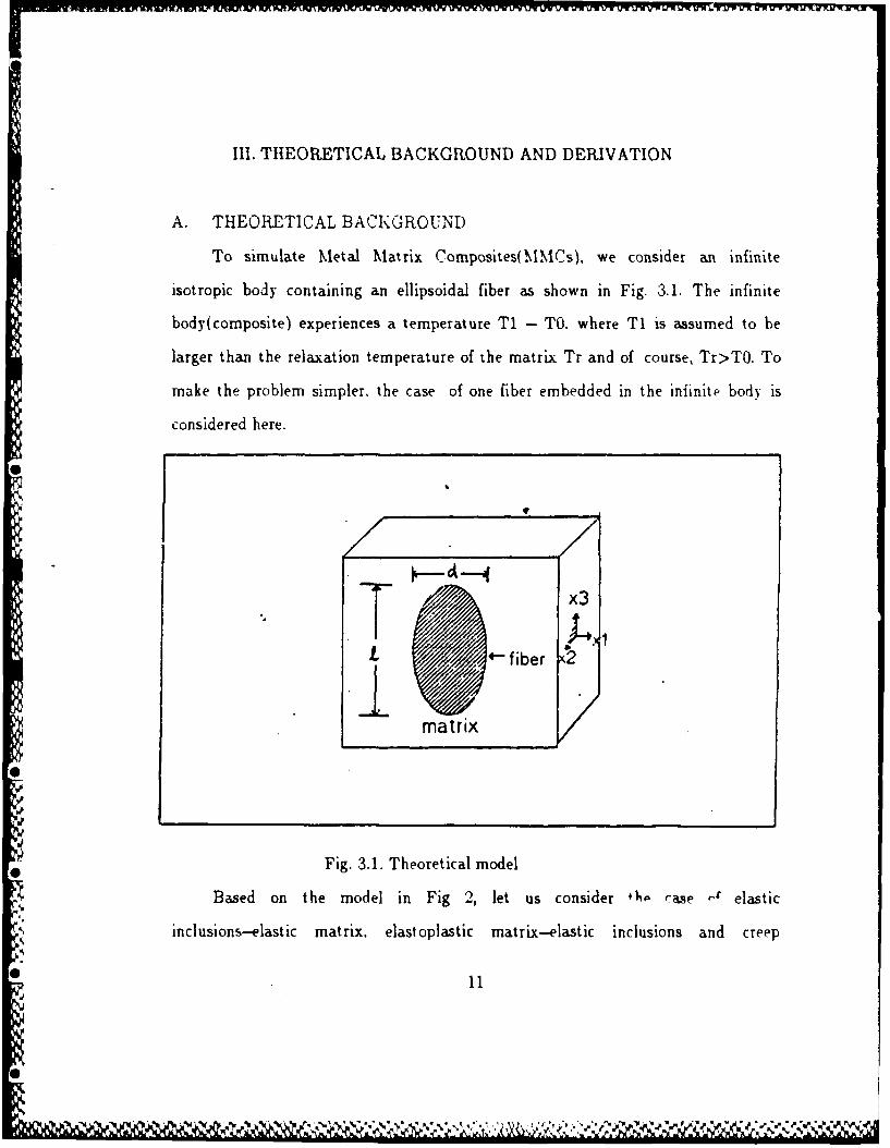
To simulate Metal Matrix Composites(MMCs), we consider an infinite

isotropic body containing an ellipsoidal fiber as shown in Fig. 3.1. The infinite

body(composite) experiences a temperature T1 - TO. where T1 is assumed to be

larger than the relaxation temperature of the matrix Tr and of course, Tr>TO. To

make the problem simpler. the case of one fiber embedded in the infinite body is

considered here.

0A

*-fiber 2

matrix

Fig. 3.1. Theoretical model

Based on the model in Fig 2, let us consider *,' cae " elastic

inclusions-elastic matrix, elastoplastic matrix-.elastic inclusions and creep

% 11

0h

deformation:

1. Elastic Inclusions and Matrix

First let us consider the average internal constrain strain E-C. To find

E.' )we insert Equation(l) and Equation(3) into Equation(4) and find

E =(1-f)S E T + fE T, which represents the average internal constrain in any" ~ijkl ki j..

inclusion in terms of transformation strain. Next, the average internal stress in any

inclusion can be represented by Equation(5). Here, E. T is an unknown term.ij

Therefore, to find this unknown term we must consider Equation (6) and Equation

(I). In Equation (6), * represents the inclusion, and ET * represents the uniformT

transformation strain for every inclusion. Once we have determined E , according1]

to the Equation g - fE T we can determine the overall strain of the specimen, andij i '3

in accordance with Equation(7) we can determine the uniform transformation E .j

•.. Elastoplastic Matrix and Elastic Inclusions

The case for elastoplastic matrix-elastic inclusions is different from that

of elastic inclusion and matrix. This is due to the fact that in this case plastic

deformation occurs only inside the matrix, so we must consider the plastic strain in

the matrix. Therefore we can find E P in accordance with Equation(6) and

Equation(lO). From Eel = e IfoC.E we can represent oP=F(E,) andTi

1) Ij

ET=F(E.P). After representing them this way,i ii

Eel = 1- iIT

Y , , 2 2=C1Ep + C2Ep(a -a)AT+C2E p(a -a) &T (14).

12

*+ K Il -I J IM HIsM + II ., a, i .... +

Differentiating this with respect to EP, we can obtain the value of Ep as shown

below:

Ep= ( -a)&T 1-f)cry ( 15)

Therefore, using the value of E to find the value E.P, the value of or-I can beIj ij

obtained, and inserting this value into Equation(16), we are ultimately able to

obtair' the total average stress in the matrix.[ref 9]

< T-I > - C < > - f (- ( 161] m ijkl kI "R

3. Creep

Applying the value of the internal stress(above) to Equation(13). we can

determine creep deformation. Following from this theoretical base, let us first

calculate mathematically the thermal residual stress of Al/SiC MMCs.

B. DERIVATION

1. Elastic Inclusions and Elastic Matrix

*First let us calculate E T for the case of elastic inclusions and elastic matrix.

In order to determine E .T, we rewrite Equation(4) in matrix form:

E j S11 S,2 S,3 S,4 S,5 S,6 E I E 1VEz [S21 S22 S23 S24 S25 S26 IE2~ E2

EM E, SSI S32 S33 S34 S35 S36 E3. +| f E3Et 41 S s42 S43 S44 S45 S46 Ed Ei 4

SS 2 S53 S54 S55 S56 EEE6S6 1 S62 S63 S64 S6 S66j E61 J E6~

13

Simplifying this matrix we obtain:

Ei1 El Sif + Si2 Et + S 13 E3h - EI- S1E+E 22 + f ) + S2,3E

3 =(if) S3iE, +S 3 2 E2 1 + Eb~ S33+ + f 3Eii E44(S 44 + f ) 4

E EIS + f ) E5~L Q6 j E6 (S66 + f ) LE61

Further, simplifying this matrix we find:

Ell = EII(1-f)Sii + E2AS 12(1-f) + EAS13(1-f) + fEi

E2 = E11(1-f)S2 1 + EAS 22(1-) + E3 S23(1-f) + fE21

E-3= E1I(1-f)S31 + EAS3(1-f) + E3AS 33 (1-f + fE3S0c

E-44 = E4(1-)S 44 + fE4CE-s= E5j(1-f)S55 + fE5t

E6 = E6k(-f)S66 + fE6t (17)

Refer to Appendix (A) for the values of Siid.

Next, let us rewrite Equation(6) in matrix form.

p- -

V - .V) V 0 0 Eij E

G v v -z) 0 0 0 ii -,Es

0 0 0 A 0 0 Eit E4).

V ( 0 0 ) 2 0 1 Eb

'(1-a')( V a' 0 0' f] 1Ea' (-aV) v 0 E2~*

H P P (1-v o 0 0 p E3I *

1Ei E4 *0i 0E0 0 0211 E66 E61

* 14

Simplifying the above matrix, we have the following-

E-j',( 1-v)J+Eic2vJ+E jc~vJ=( 1-v)GE ,t + tPGE 24+VGEsk1-v)HEA*

, HEA- -HE.j

E11 vJ+E2jc( 1-v)J+Ej3c3VJ=zGEI + (1-)GE2 +VGEA-vHEa -

(1-v)HEAi* -HEs 3 *c*

Eic vJ+E2-iJ+Es( 1-.v)J=v GE, + YGE21+( i-z)GE4 -vHcd-

,vHEA *- (1-iv)HE31

-CE44 =0

-CE55 = 0

TFrom Equation (17) and (18), if we simplify and solve for E we obtain:

KE41LE&~ME3 =-( 1-t)HEtI * -H4-i'HEA*

* NEI+PE2A+QE 3 =-,vHEdI--i ,)HE2A*-vHE 3 *

*REij+SE21+TEsh=-YHjvHEA * 1-v)HEA*

Ej= Edl

E5J = Et

Q = (-a*(19)

Now, we have 6 unknown values and 6 Equations. Therefore, applying Equation(19)

to determine E T:

El=-YL - XM - HA (1-;,)

1.5

E2A= W - VXUEA=_, zu - xwUX - xv-

E, = EXE5 = j*

A = EX* ( 20)

Putting the above equations into simplified form:

ij E4 E44I -E E5fl E5

Here, refer to Appendix(C) for constants B through Z. Thus, inserting the value

E T into Equation(5), which is the average internal stress in any inclusion, we canii

determine the internal stress.

-1 V v 0 0 0 - BZI+CYI+DXl-Z'O22 1 I (1-v) 0 0 0 CZ'+BY'+DX'-Y'053 =G (1-v) 0 0 0 FZ'+FY'+EX'-X'o; 410 0 0 2p 0 0'!5I 1 00002 060 0 0 0 0 2p 0

2. Elastoplastic Matrix and Elastic Inclusions

Up to this point we have found the internal stress in the case of an

elastic matrix and elastic inclusions. Now we will consider the case of elastoplastic

matrix and elastic inclusions. Here also the method of determining the internal

AL6

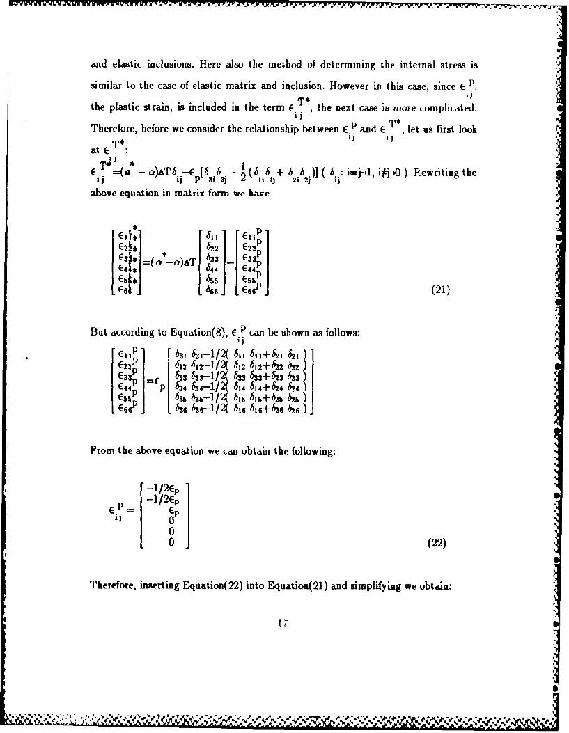
and elastic inclusions. Here also the method of determining the internal stress is

similar to the case of elastic matrix and inclusion. However in this case, since E.P,T* I)

the plastic strain, is included in the term E.. , the next case is more complicated.ap T*

Therefore, before we consider the relationship between E.. and E , let us first lookIi iiat E T * .

ati )

E T*=(a- a)T6 -E 6 6 b( 6 + 66.)] ( b..: i=j--l, i j-.O). Rewriting theij P N 3j liIj 2i 2j 1)

above equation in matrix form we have

E2 622 E2

E3 _3 E33 p

But according to Equation(8), E.p can be shown as follows:E,,p ] b, b ,-11 b, ,+12 ' ,

E22 p - 612+62 2

E33p E b3 6,.-1I2( 633 h3+ 623 623

E44[ P634 634-1 b14 614"+-24 b24

E66 p 1 6 36-1/1 b,6 6,6+626 6526

From the above equation we can obtain the following:

.- 1/2Ep

p -1/2EpEij EP

0 j(22)

Therefore, inserting Equation(22) into Equation(21) and simplifying we obtain:

17

I

-• , • V Wj Vt'

E T*=(a* - a)aT + Ep/2I I

E T*=(a a)AT + Ep/222

E T*=(a -a)&T- Ep33

E T*=044

E T*=055

E T*=0 (23)66

Next, using Equation(4) and Equation(6), if E.. is expressed as EA, the result is theI j Tsame as Equation(17). Inserting Equation(17) into Equation(6) and expressing E

as E T* we obtain:1

ET= T* T* T*=Q~11 QE 22 - QE 3 .

ET2 P4ETI+P 5E2 2 + P6E3 3T= T* T*

E T PIEIT*+ P 2E2T + P 3E3 333E T=0

44ET=

55E T=0 (24)

66

Next, in order to find EAI, we insert the value of ET into Equation(14) and simplify:

.c T* T*+ RET*

* E-A=RET,+ R2E 2 F 3sEi2=R E* +RE + T*

-c T* T* T*E s=R 7E1 + I g 2T + RgE'?

E44=0E 5j=o

0"1

E66=0 (25)

I-Therefore a ] can be found in accordance with Equation(5). (The value of this arij is

different from the value of ao7 for elastic inclusion and elastic matrix, the reason

4being that ui for elastic inclusion and elastic matrix does not contain E.P). Here, ini

order to determine the value of aij we must first find the value of Ep. From

Equation(10), if we differentiate Eel with respect to E we can obtain Equation(11).

Therefore, from 6Ei =[ 2C, E + C2(a* - a)AT]JE and -6EeI = (1-f)oy Ibp , wep p y p

can obtain the value of E P. Again, inserting this value of E p into Equation(22) we

can find the value of E.P. Finally, by inserting the value of E .p into equation(27) we

4 i ij

obtain the value of O'i. Utilizing Equation(10) again to find the value of Ep

It 1 El * XAI' + X2Ep A' + Ep/20221 E2 * X3A' + X4Ep A' + E/2

Eel= - 1 0 1 E3 * =_ XA' + Up A - Epif044 1}E4I*] iF 1arb l E51 * 0 0.0 6 J 0 0

- [E X-T+7 - X6 ) + EpA'( j'+X 2+ +, X4-X 6+XG)

+ A12( XI+X 3+X5 ) (26)

Therefore, differentiating Eel in respect to Ep:

bEel =( C2A' + 2EfpC )6E (27)

And inserting Equation(27) into Equation(11) and simplifying obtains:

f( C2A'p+ 2EpCI )6Ep=(1-f)Oy (28)

19

If we find the value of Ep from Equation(28).

Ep=--2,(a -a),TT2{1-f)o'y (27)

( +: kp <0 - Cooling, -: Ep>0 - Heating)

If this value of Ep is inserted into Equation(24) and (25), the value of E.. and the

value of E C can be found, and if these values are inserted into Equation(5) the value

of o- can be determined. Therefore, inserting this value into Equation(16) we areii

ultimately able to obtain total average stress in the matrix. Refer to Appendix((")

for the constants and actual values.

03. Creep

Up to this point we have been determining the internal stress both in the

case of elastic matrix and elastic inclusion and in the case of elastoplastic matrix

and elastic inclusion. But in these two cases the actual effect on creep deformation is

the internal stress in the case of elastoplastic matrix and elastic inclusion.

Accordingly, by inserting the value of the internal stress into Equation (13), we can

plot the microcreep deformation phenomenon as a function of time as shown in Fig.

3.2. Refer to Chapter IV part A for more detailed information.

2(1

V4-

L fV

FIG.3-21Micr~ree &s funtionof tme

210

IV. RESULTS AND CONCLUSIONS

A. RESULTS

The thermo-mechanical data of the matrix and fiber for the theoretical

calculations are obrtained from the [ref 13].

Annealed 2024 Al matrix:

Em = 47.5 GPa

= 47.5 MPa

= 0.3

a = 23.6x10/ K (31)

SiC fiber:

Ei = 427 GPa

f =0.2

a = 4.3x10--6/K

l/d= 1.5 (32)

Where the average value of the fiber aspect ratio(l/d) was used [ref 13]. The

temperature drop aT is define as

&T = T1 -To (33)

Where T1 is taken as the temperature below which dislocation generation is

minimal during the cooling process and To is the room temperature. Thus, for the

present composite system aT is set equal to -200K. From the data given by

Eqiation (31), (32) and the use of < 01.. >_ = -f(I we have computed the stresses.

Next, the thermal residual stresses, averaged in the matrix of SiC fiber/2024 Al, are

22

predicted by (17) and the result on < -I >. as plotted in Fig.6, where 33 denote

the component along the longitudinal direction(z). The average theoretical thermal

residual stress is predicted to be tensile in nature, and the average residual stress in

the longitudinal direction to be larger than the average residual stress in the

transverse direction [Table 5]. The fiber aspect ratio(cr-i/d) of SiC fibers has been

observed to be variable [Appendix A,B]. In the present model we have used the

value of lI/d, 1.5 to predict the thermal residual stress of the romposite.

TABLE 1: The value of E.P (a=1,1.5)ij

u(l/d) E P E P E P1II 2 33

1 -0.0017 -j. 0017 -0.0017

1.5 0.0014 0.0014 -0. 0026

T*TABLE 2. The value of E i i (0=-l, 1.5)

o Id) ET* ET * ET*

1~/d I 22 3 3

1 0.0056 0.0056 0.0056

1.5 0.0025 0.0025 0. 0066

2

232

TABLE 3: The value of Eii (0=1, 1.5)

a( I/d) E E E_ _ _ _ _I I 22 .3,11

0.0053 0. 0053 0.0053

1.5 0.0025 0.0025 0.0060

TTABLE 4: The value of EiJ (a=l, 1.5)

a(l/d) E T E T E TII 22 33

1 0.0076 0.0076 0.0076

1.5 0.0025 0.0025 0.0115

TABLE 5: The value of t7.. (a.--, 1.5)-1 -

o(l/d) tT (MPa) c---(XMPa) & -(NMPa)________2? 33

1 -276.23 -276.2 3 -276.23

1.5 -154.82 -154.8 2 -154. 8 2

TABLE 6: The value of <6!>- (r1, 1.5)

a I /d) <01- >(MIPa) <01-I>(MPa) <o-I>(MPa)

________Ii22 33

1 55.245 55.245 55.245

1.5 30.905 30.905 70.998

24

U

0

TABLE 7: Comparison value of < r >. , with TODAY'S

a(I/d) OUR MODELS' S TAYA'S____< uT-3 >,,(MPa) < t&3 >,(MPa)

1.8 71. 156 67.894

As seen in tables 1. 2, 3, 4, 5, 6, and 7 we can observe that as a increases, the values

P T* "c T-I of Ei , E , El, Ei j u~, and < uj >, also increase.

.p.

,"

'

25

W W~

I

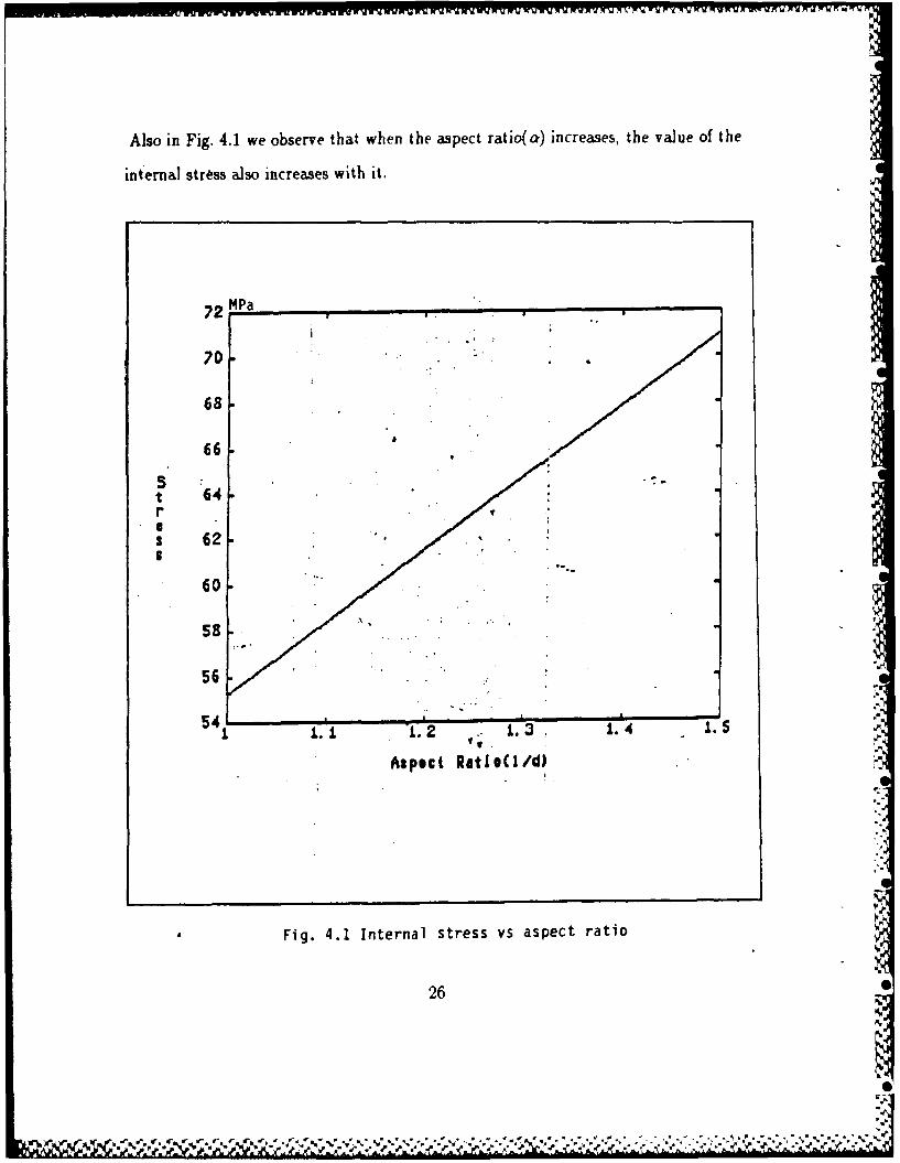
Also in Fig. 4.1 we observe that when the aspect ratio(a) increases, the vaJue of the

internal stress also increases with it.

22 Pa .

70 C

683

66

56564

54r .,2 3 L.4 -. S

•Aspect Ratlocl /d)

Ii

Fig. 4.1 Internal stress vs aspect ratio

26

26 ro

7"

- i~hCi)-u¢'W"i¢u rz". €,,rar W, ac,.ru

e •,,- "%"%-, . " = ."%",, , % ' ... = _ .• -, .,,-• . . . . %.,, . . .a%,% , 0

And in Fig. 4.2 we can also see that the value of the internal stress increases with an

increase in temperature.

1 3 0 1 M f a...

120

110

100St

80 V

80

60.

00 10 200 250 300 350 400

Temperature change(delta T)

Fig. 4.2 Internal stress vs temperature change($aT)

27

In Fig. 4.3, in the case of an ellipsoid (a=.5), the values of internal stresses

increase with an increase in volume fraction,

- 2 -Pa

70

68

66 -5

r 64

60

S B58

626

0. 12 0. 14 0. 16 0. 1S 0.2

Volume fraction

~1

* Fig. 4.3 Internal stress vs volume fraction(f)

28 1_0 L

Next, if we compare the theoretically predicted value of the internal stress with the

value determined by R. J. ARSENAULT and M. TAYA, we see that our mod's

value is larger than the value which is obtained by R. J. ARSENAULT and M.

TAYA, as shown in Table 7. They used the material properties as follows:

Annealed 6061 Al matrix:

E=47.5 GPa

ay=47.5 MPa

1/=0.33

=23.6x10 -'/K

SiC whisker:

Ei=427GPa

f =0.17

a =4.3x10 -6 K

l/d=1.8

Finally, Fig. 3.2 is a graph showing the strain as a function of time, when th,- aspect

ratio is 1.5 and the value of the thermal residual stress is inserted ir'"-

Equation(13). If we analyze Fig. 2.3 we can see that the creep deformation

phenomenon is due to the internal thermal residual stress of the MMCs.

B. CONCLUSIONS AND RECOMMENDATIONS

The object of this research is to obtain the value of the thermal residual stress

of an Al/SiC composite using Eshelby's theoretical model, and then to determine

what effect this thermal residual stress value produces on creep deformation.

Because exact creeping behavior of this material is difficult to determine when

analyzing creep deformation, Andrade's model was used with properly selected

29

N

constant values. But through this theoretical approach the following co, lusions can

be obtained.

1, Thermal residual stress due to the difference in thermal expansioncoefficients may be estimated.

a. By means of the theoretical model, we can see that the thermalresidual stresses increase when the volume fraction of the inclusionsincreases.

b. In the case of sphere inclusions, that is, when the aspect ratio cr=l, thelateral stress is equal to the longitudinal stress.

c. In the case of an ellipsoid inclusions where a=1-.5 the longitudinal stressis greater than the lateral stress.

d. The thermal residual stresses of Al/SiC composites increased whenthe value of the aspect ratio of the inclusions increases.

0 2. Microcreep deformation can be estimated in the model by using thethermal residual stresses and the Andrade's model of creepdeformation

a. Microcreep deformation is due to the internal thermal residualstress of the MMCs.

b. Dimensional stability of comp,n-nts will be influenced by the

behavior of the composite.

3 Recommendations

a. Presently, this thesis has only dealt with average thermal residualstress from a overall point of view. and we need more detailedlocal residual stresses surrounding SiC particles should beestimated for analyzing creeping behavior.

b. In the future, research should be done concerning relaxation duringcooling.

c. The creep b'-havior used in the current model is the Andrade'sapprox.' ,.ation. The real creep deformation for this Al/SiCcompos,.e should be further studied in order to get betterunderstanding of the microcreep of the material based onapproximation values.

.30

• ,,

APPENDIX A

PROGRAM FOR VALUE OF Sikl(,=l.S - 5)

1. PROGRAM(FORTAN)

RZjA*8 KU ALP G, TP,S1111,3333 S1122, S1133 ,S3311NU-0. 3WRITE (6,*90).WRITE (6,*95)ALP-1.5

300 TKP-ALP**2-1.G-(ALP' (ALP'DSQRTCTNP)-DLOG(ALP+DSQRT(TMfP))) )I(TMP**(3./2.))Sllllm(3.'ALLP"2)/8.C1.-NJ)T?)

4 *++(1.-2.*NU-9./(4.*T34P))*G/(4.*(l-NU))S3333-((l.-2.*NU+(3.*ALP**2-1.)/T(P-(1.-2.*'NU+3.*ALP**2/TMP)

+*G) )/(2.' (l.-NU))S1122-(ALLP**2/(2.*TP)-(.-2*NU).3*G/(4.*TP))/(4.*2.-NU))S1133-ALP**2/(2.*C1.-NU)*TMP)+C3.OALP**2/TMP-(l.-2.*NU))*G

+/(4.* (1.-NU))

S331G/(2. l.-2.NU /TP)(.(*-U)+(. 2*U3/2*M)

* WRITE(6,100) ALPSllll,S3333,Sll22,Sll33,S3311ALP-ALP+.1.IF(ALLP.GT.5.) GOTO 400GOTO 300 to' L 1 1*90 FORKAT(1.X. S3333; S1122 S1133

+ S3311')95 FORMAT (1X,' mmmmmmnmmmmmmmmmmmmimiium

100 FORMAT(1X,6(F10.5))400 STOP

END

31

2. Sijkl VALUE WITH ASPECT RATIO

ALP Sli1 S3333 31122 S1133. S3311

1.50000 .58078 .39378 .01421 .08396 .019451.60000 .58828 .37371 .01603 .08992 .016231.70000 .59495 .35518 .01764 .09549 .013501.80000 .60089 .33804 .01906 .10071 .011171.90000 .60620 .32215 .02032 .10560 .009182.00000 .61098 .30739 .02145 .11018 .007472.10000 .61529 .29366 .02246 .11448 .006002.20000 .61920 .28087 .02337 .11851 .004722.30000 .62274 .26893 .02419 .12231 .003622.40000 .62598 .25777 .02493 .12588 .002662.50000 .62893 .24732 .02560 .12924 .001832.60000 .63164 .23752 .02622 .13241 .001112.70000 .63412 .22832 .02678 .13540 .000482.80000 .63641 .21967 .02729 .13822 -.000072.90000 .63851 .21152 .02776 .14090 -.000563.00000 .64048 .20384 .02819 .14342 -.000983.10000 .64229 .19659 .02859 .14582 -.001343.20000 .64397 .18974 .02896 .14809 -.001673.30000 .64554 .18326 .02930 .15025 -.001953.40000 .64700 .17713 .02962 .15230 -.002193.50000 .64836 .17131 .02991 .15425 -.002413.60000 .64963 .16579 .03019 .15610 -.002593.70000 .65082 .16054 .03044 .15787 -.002763.80000 .65194 .15555 .03068 .15955 -*002903.90000 .65299 .15081 .03090 '.16115 -.003024.00000 .65398 .14629 .03111 .16269 -.003124.10000 .65491 .14197 .03130 .16415 -.003214.20000 .65579 .13786 .03149 .16555 -.003294.30000 .65662 .13393 .03166 .16689 -.003354.40000 .65740 .13018 .03182 ,16818 -.003404.50000 .65814 .12659 .03197 .16940 -.003454.60000 .65884 .12316 .03212 .17058 -.003484.70000 .65951 .11987 .03225 .17171 -.003514.80000 .66014. .11671 .03238 .17280 -.00353'4.90900 .66074 .11369 .03250 .17384 -.00355

32

APPENDIX B

PROGRAM FOR VALUE OF S ijk(a=1.O-,

1. PROGRAM(MATLAB)

%SPHuRZ (ALPHA-i.O0)

f or 1-1: 6;numi/lO.;den-15. *(1-nu);sll(i)-(7-5*nu)/don;*.12(i) -(5'nu-l) Idmn;s2.3(M)-s12(iM

* s3l(i)-al2(i):s33(i)-s11(i);

%V

ULLPHA-MNINITY

den2-8'(1-nu);ssll(1) 'C5-4. 'nu) der&2;ssl2 (i)ft(1-4*nu) /den2;as3(i)mnu/(2.*(l-nu));ss3l(i)-&O;ss33 (i)mO;end;resultlum~sll;sl2;sl3:s3l;s33;J'result2m~ssll;ssl2;sal3;ss3l1;ss33]'

03

aL

2. Siikl VALUE

S1l S12 513 S31 S33

resultl -

C.1 0.4815 -0.0370 -0.0370 -0.0370 0.48150.2 0.5000 0 0 0 0.5000

0.3 0.5238 0.0476 0.0476 0.0476 0.5238

C.4 0.5556 0.1111 0.1111 0.1111 0.5556

0.6000 0.2000 0.2000 0.2000 0.6000

C. 0.6667 0.3333 0.3333 0.3333 0.6667

result2 -

0.1 0.6389 -0.0833 0.0556 0 0

0.2 0.6563 -0.0312 0.1250 0 0

0.3 0.6786 0.0357 0.2143 0 0

0.4 0.7083 0.1250 0.3333 0 00.5 0.7500 0.2500 0.5000 0 00.6 0.8126 0.4375 0.7500 0 0

34

A

*>. *~

0

APPENDIX C

PROGRAM FOR VALUE OF THERMAL RESIDUAL STRESS,

P T* -I] i j >m

1. PROGPIAM(MATLAB)

%This program computes stress values and constants

%Initial valuesN

nu-Q.3;e.-47.5e9;ei=427. 09:sym47.506;f-0.2;

* dt--200ap-23.6e-6;as-4.3e-6 ;mu-0.;

%Eshelby's tensor components

sll-0.6786;s33-0.0000;s12-0.0357;sl3m0.2143;s31-0.0000;

% Constants

: h-,ei/((1. nu)*t(1.-2.*nu)) ;

" "~i (.a-ei) / ( 1. nu) * (1.-2. "nu)) ;* am-tol21'(1.-f) ;li b-s12' (1.-f) ;

c-s13**(1.-f); .

d-a31 (1.-f);

35N

-,,.-v ,~~ ~ .\.%%:

continued

tl-rl+r2+r3-ql+q2+q3:t2- (rler2-2'z3) /2.- (ql-q2+2*q3) /2.;t3-r44r5+r6-p4-p5-p6;t4-(r4ir5-2'r6) /2.- (p4+p5-2*p6) 12.;t5-r7+rB+r9-p1-p2-p3;t6- (r7irS-2'r9) /2-7(Pl+p2-2*p3) /2.;x1.q* ((1.-au) 't14Wz'(t3+t5));

x3wgO ((1.-au) 't3enu'(tl+t5));x4-g' ((1.-nu) 't4+nu' (t2+t6));

x6-g' ((1.-au) 't6+n4' (t2+t4) ):clm((x2+x4)/2.-x6)*(f/2.);c2-( (x1+x3)/2.+x2tx4-x+x6)(f/2.);

% Temprature dependent.-para&motor%ftv

ep--c2*app/(2.*cl)+(1.-f)asy/(2.*cl);

% Blastic moduli of the matricies

aaa-g'[(l-nu) nu nu 0 0;;u (1-au) nu, 0 0 O;nu nu (1-au) 0 0 0;0 0 0 2.*mu 0 0;0 0 0 0 2.*wu 0;0 0 0 0 0 2.'aujl;

% Plastic strain 'in the matrix

eijp-C-op/2 -ep/2 op 0 0 0].

% Uniform trnfrainsrana nlso

oiJtsmEapptep/2 app+ep/2 app-op 0 0 011

36

-- ~~ ~~'M ~ ~ :~. )TVi~w lr -' VIE WK VRV I u C1 Vr UN-

continued

eijt-Cql' (app.~ep/2)-q2' (app+ep/2)-q3' (alpp-epIp4* (appiep/2)+p5 (app+ep/2)+p6 (aPP-eP)p1l (app+ep/2)*p2* (app+ep/2)+p3* (app-ep) 0 0 03

eiJ...czrl(pep/2)+r2(app+p/2)+r3 (aPSPo)r4*(app+ep/2)+r5*(app+ep/2)+r6 (app-0p)

r7etapp~..p/214+rS*(app+ep/2)+r9St(aip-6p) 0 0 02

% Xverage internal stress in inclusion

sij i-aaa (ei j~c-eijt)

% Average stress in the matrix

sijmo-t aijji

37

4-

2. CONSTANTS OF ELASTIC MATRIX AND ELASTIC INCLUSIONS

B=S11 ( i-f) + S 1-S2( 1-1 + f

DS31-f) E=S 33( 1-f) + f

F=S31( 1-f) G=Em/(1+i,)( 1-2i')

K=J(( 1-v)B-i-iC+vF)-(1--v)G L=J(( 1-v)C+vB+vF)-YG

M=J(( 1-iz)D+ivD+i'E)-iG N=J((1-i',)D+iD+ivE)-z'G

P=J(( 1-i)B+vC+vF)-41-')G' Q.J(( 1-ti"D+,'D+i',E)-ivG

13=J((1-i',)F+vB+I')-i/G, S=J(( 1-v)F+iiC+'B )-vC'

Y'=J(( 1-i')B+2i'D )-( 1-03G U=(PK - NL)/K

EV=(QK - NM)/K W=A H(1+i/)(N-K)/K

X=(SK -RL)/K) Y=(TIK- MR)/K

Z=A H( 1+z)( R-K )/K X =( ZU-XW)/(UY-X\V)

Y =(W-X v I/U Z =(-Y L-X M-HA(1z)/

I3

Copy ac~jL1', I' i notV.eru it fully legible z roducion

APPENDIX D

FORMULA OF SijkI FOR A VARIETY OF INCLUSION

1. FORMULA OF S ijkl(a=1.5 - 5)

3. 121 9_____811l - v) lu- - 1) 4(1 -&'~ IS1 )I

SII 2 + -I. -.4(1a - ___ __

411 +vo 2{&I-- ) 2&t- -+ 3*,-2(1 - vo) ( - 11

3 n212 ~ (-w - -

'1 S2211___ (I-2 o

40-jo 2(ir + 1)"1:1. S S2233 = - +

2(1 -vo) (at 1) 411 1~ (r-I

'51-31 = SAX22 = ( i- 2jo + -

+ 1 - 2v + ""

2(1 - 2(cT. - III

where v is Poisson's ratio of a matrix. ty is aspect ratio ol a fiber

(-I1d). and g is given by

g = lata2 - 1 rl - cosh- ' iJ1)V2

39'S,

0

2. FORMULA OF S~ik(al=l)

122=7 V7T5?

S - - 51'2222 T5Urw71

2 233 TTTUY-7

3312 7 v-1

5v -

400

3. FORMULA OF S ijkl(c-)

s 5 - 41/

S -- 4v - 1

* 8( - u

Is 5 - 4vS =

S 0* 3311

S =03322

S= 03333

41

. . ... .* .....* *.

A TEN 1)IX F,

PIMOFliAM M~i. CIF1',IEF ORMIATION

PlIOGRAM( MATLAB)

epO- . 001;beta-0.0465;)c7.2e-7;for tl:91;kv(tt)=tt;

eep(tt)=epoa (l.+beta't- (1/3)) uexp(k't);.end;plot (kv, eep)semilogx;xiabel(VTime t'),ylabel('Strain eps')

42

LIST OF REFERENCES

I. CHU-WHA LEE, "Thermal residual stress in Al/SiC Metal MatrixComposites and the influence of their viscoelstic and plastic relaxation ondimensional stability". RESEARCH PROPOSAL

2. J. D. ESHELBY, "The elastic field outside an ellipsoidal inclusion". "Thedetermination of the elastic field of an ellipsoidal inclusion, and relatedproblems". DEPARTMENT OF PHYSICAL METALLURGY,UNIVERSITY OF BIRMINGHAM. PROC. R. SOC. A242. 1957

3. K. WAKASHIMA, M. OTSUK and S. UMEKAWA "Thermal expansions ofheterogeneous solids containing aligned ellipsoidal inclusions". J

COMPOSITE MATERIALS, VOL.8. 1974

4. R. I. ARSENAULT and M. TAYA, "Thermal residual stress in MetalMatrix Composite". ACTA METAL VOL.35 No.3 1987.

5. LEIF LARSSON and VOLVO, SWEDEN "Thermal stresses in MTMCs"CSDL MMC PROGRAM CONSOLIDATION STRESSES

6. METAL HANDBOOK. VOL.8

7. M. TAYA and T. MURA, "On stiffness and strength of an alignedshort-fiber reinforced composite containing fiber-end cracks under uniaxiaiapplied stress". JOURNAL OF APPLIED MECHANICS, VOL.46 JUNE1981

S,. P. J. FRITZ and R. A. QUEENEY "Visco elastic and plastic relaxation ofresidual stresses around macroparticle reinforcements in metal matrices".(OMPOSITES. VOL.14, OCT.1983

9. T. MORI and K. TANAKA, "Average stress in matrix and Average elasticebergv of materials with misfitting inclusions". ACTA METALLU;RGICA.VOL.21, MAY 1973

10. Y. FLOM and R. J. ARSENAULT, "Deformation of SiC/Al composites".JOURNAL OF METALS, JULY 1986

11. TOSHIO MURA and M. TAYA, "Residual stresses in and arlind a shortfiber in MMCs due to temperature change". RECENT ADVANCES INCOMPOSITES IN THE U.S and JAPAN, 1%5

12. L M. BROWN AND D. R. CLARKE, "The work hardening of fibrous

composites with particular preference to the COPPER-TUNGSTENsystem". ACTA METALLURGICA. VOL.25. 1977

43

'Siv ', ,wJ*'"2"g,.,J"J¢2',, U' _,2,. , ¢JJ.:r".*,"- , .J "*. - _ - - - -- . ,¢ ,,, ' '.'

13. MARY \OGELSANG, R. J. ARSENAULT, AND Ft. M. FISHER "An INSITU HVEM study of dislocation generation at Al/SiC interface in MMC.METALLURGICAL TRANSACTIONS A. VOL. 17A 1966

44

4t

INITIAL DISTEIBUTION LIST

No. Copies

1. Defense Technical Information Center 2Cameron StationAlexandria, Virginia 22304-6145

.2. Library, Code 0142Naval Postgraduate SchoolMonterey, California 93943-,5002

3. Department Chairman, Code 69Department of Mechanical EngineeringNaval Postgraduate SchoolMonterev. California 93943--5004

4. Prof. Chu Hwa. Lee Code 69Department of Mechanical EngineeringNaval Postgraduate SchoolMonterey, California 93943--5004

,5 Prof. Terry R. McNelley Code 69Department of Mechanical EngineeringNaval Postgraduate SchoolMonterey. -alifornia 93943-5004

6. Jung, Yun Su1.50Yon g-Deung po Gu, Yang-Pyung Dong, 4 Ga, 27Seoul, Korea

7. ri, Chang-Ho160-01In-Cheon Si, Nam Gu, Seo-Chang Dong, 170Seoul, Korea

8. Lt. Col. Hur, Soon Hae 5151Dong Jack Gu, Shin Daebang 1 dong600-28, 14 Tong 2 Ban Seoul, Korea

9. Maj. Wee, Kyoum BokSMC 2814Naval Postgraduate SchoolMonterey, California 93943-5000

45

!!

[ W ~ x"XK-NWU- '-' 7V N-VVV r21,'.7 7 N-~J, .~ 1 i ~ Ti w - %i~ -N~L7 11Lv-7Nw" x.7'k lv. % v., ,~* ~W

10. Maj. Yoon. Sang I]SMC 1558Naval Postgraduate SchoolMonterey, California 93943-5000j

11. Cpt. Han, Hwang JinSMC 2402Naval Postgraduate SchoolMonterey, California 93943-5000

12. Maj. Kim. Jong RyulSMC 1659Naval Postgraduate SchoolMonterey, California 93943-5000

13. Lee, Yong MoonMa-Po Gu, Yun-Nam Dong, 382-17Seoul, Korea

14. Cpt. Song, Tae IkSMC 2686Naval Postgraduate SchoolMonterey, California 93943--5000

15. Paul B. Wetzstein1206 Inchon CourtFt. Ord, California 93941

16. Naval Surface Weapons CenterWhite Oak LaboratoryATTN: Dr. Han S. Uhm (R41)10901 New Hampshire AvenueSilver Springs, MD 20903-,000

17. Naval Surface Weapons CenterWhite Oak LaboratoryATTN: Dr. Donald Rule (R41)10901 New Hampshire AvenueSilver Springs. MD 20903-5000

46

i'-