RJH/H4 Igneous Mineralogy: Solid Solutions and Phase Diagrams 1

http://www.esc.cam.ac.uk/~rjh40/overheads.html

Natural Sciences Tripos Part 1b

GEOLOGICAL SCIENCES B

Igneous Mineralogy

Richard Harrison

Solid Solutions and Binary Phase Diagrams -----------

Olivine Minerals

RJH/H4 Igneous Mineralogy: Solid Solutions and Phase Diagrams 2

Introduction A solid solution is a single phase which exists over a range in chemical compositions. Some minerals are able to tolerate a wide and varied chemistry, whereas others permit only limited chemical deviation from their ideal chemical formulae. In many cases, the extent of solid solution is a strong function of temperature – with solid solution being favoured at high temperatures and unmixing and/or cation ordering favoured at low temperatures. Here we discuss relatively simple binary solid solutions, where the chemical composition of the mineral can be specified in terms of just two chemical components. The equilibrium behaviour of the system as a function of temperature and composition is specified by a binary phase diagram, and we will spend some time learning how to derive and interpret binary phase diagrams for different types of binary solid solution. Many of the concepts will be illustrated here by reference to the important igneous mineral olivine.

General concepts you definitely need to know! By the end of these two lectures you should: i) know the different classifications of solid solution

ii) know what factors control the extent of solid solution tolerated by a mineral

iii) know what is meant by the terms ideal and non-ideal solid solution

iv) know what is meant by the enthalpy, entropy, and free energy of mixing

v) know what is meant by the terms exsolution and cation ordering, and under which circumstances these processes might occur

vi) understand how to interpret binary phase diagrams. vii) be able to describe the sequence of events during equilibrium heating and cooling through a

phase diagram and apply the lever rule viii) know what is meant by the terms eutectic, eutectoid, peritectic, and peritectoid point,

congruent and incongruent melting

What you need to know about olivine! i) be familiar with the structure and chemistry of the olivine minerals ii) know how to identify olivine in thin section iii) know how to determine the composition of olivine in thin section using 2V iv) be familiar with the geological occurrence and significance of olivine, especially with

respect to the occurrence and behaviour of olivine in the mantle

RJH/H4 Igneous Mineralogy: Solid Solutions and Phase Diagrams 3

Olivine M2SiO4 Structure The olivine minerals have the general formula M2SiO4, where M is most commonly Mg or Fe2+. The structure belongs to the orthorhombic crystal system with space group Pbnm (crystal class mmm). This space group symbol specifies a primitive lattice with a b-glide plane parallel to (100), an n-glide plane parallel to (010) and a mirror plane (m) parallel to (001) (see essential crystallography handout). The structure consists of isolated SiO4

4- tetrahedra, which are held together by M cations occupying two types of octahedral site (M1 and M2). Fig. 1a shows the arrangement of SiO4 tetrahedra in a projection down the x-axis of the orthorhombic unit cell. The isolated tetrahedra point alternately up and down along rows parallel to the z-axis. There are two rows at two levels in the unit cell, the lower level (at x = 0) is drawn darker than the upper level (at x = 0.5). Note that the upper and lower rows are related to each other by the b-glide parallel to (100) (at height x = 0.25 and x = 0.75).

Fig. 1a

Fig. 1b shows the arrangement of the M1 and M2 octahedra in the lower level. The M1 octahedra share edges to form ribbons parallel to the z-axis. Ribbons in one layer are connected to those in the layer above by M2 octahedra, also by edge-sharing. Together, the M1 and M2 octahedra form a continuous 3d network. Because the octahedra share edges, rather than corners, this network cannot distort by mutual rotation (as was the case for the corner-sharing tetrahedral network

Fig. 1b

RJH/H4 Igneous Mineralogy: Solid Solutions and Phase Diagrams 4

in the silica minerals). However, the octahedra are allowed to expand with increasing temperature or decreasing pressure, and the relative size of M1 and M2 can change. The size of the SiO4 units remains virtually unchanged with temperature, as expected (the Si-O bond is much stronger than the M-O bond). The structure can alternatively be described as an approximately hexagonal close-packed array of oxygen anions, with M and Si cations occupying one half and one eighth of the octahedral and tetrahedral sites, respectively. The close-packed layers lie parallel to (100). If the hexagonal close packing is ideal, then M1 and M2 are regular octahedra and have equal size. In reality the hcp arrangement is not ideal and the M1 and M2 octahedra have unequal sizes, with M2 being slightly larger and more distorted than M1 (see Fig. 1). Chemistry The two most important forms of olivine are forsterite (Mg2SiO4) and fayalite (Fe2SiO4). These two forms have identical symmetries and structural topologies (although individual bond-lengths may vary), the only difference is the type of cation occupying the M site (either Mg or Fe2+). Most natural olivines have compositions intermediate between forsterite and fayalite, i.e. the M sites are occupied by a mixture of Mg and Fe2+ cations.

Fig. 2 This is a classic example of a substitutional solid solution, i.e. one where chemical variation is achieved by simply substituting one type of atom in the structure by another. Forsterite and fayalite are referred to as the endmembers of the solid solution and the composition is specified in terms of the mole fraction of these endmembers, i.e. an olivine with chemical formula (Mg0.4Fe2+

0.6)2SiO4 is said to contain 40% forsterite and 60% fayalite (often abbreviated to Fo40Fa60). It is crucial to consider how the mixing of Mg and Fe2+ cations is achieved at the atomic scale. In the ideal case, the Mg and Fe2+ cations are randomly distributed over all the available M sites. This is depicted schematically in Fig. 2, which shows an array of cation sites randomly occupied by one of two types of cation. The probability of an M site being occupied by Mg is equal to the proportion of Mg in the system, i.e. for Fo40Fa60 there would be a 40% probability of an M site being occupied by Mg and a 60% probability of it being occupied by Fe2+. In reality, there is a slight preference for Fe2+ to occupy M1 sites, leading to a slight deviation from ideality in the olivine solid solution. Other classifications of solid solution As well as the substitutional solid solution, there are other ways to achieve chemical variation in a mineral:

i) Coupled substitution. Similar to the substitutional solid solution, but cations of different valence are interchanged. To maintain charge balance, two coupled cation substitutions must take place. For example, the plagioclase feldspar solid solution between albite (NaAlSi3O8) and anorthite (CaAl2Si2O8) involves the coupled substitution Al3+ + Ca2+ -> Na+ + Si4+. Another famous example is the so-called Tschermak substitution, Mg2+ + Si4+ -> 2 Al3+.

RJH/H4 Igneous Mineralogy: Solid Solutions and Phase Diagrams 5

ii) Omission solid solution. Here chemical variation is achieved by omitting cations from

cation sites that are normally occupied. For example, the pyrhottite solid solution Fe1-xS varies in composition from FeS to Fe7S8 by creating cation vacancies. Charge balance is maintained by converting some of the Fe2+ to Fe3+. Such solid solutions are also common in the Fe-oxide minerals (e.g. the solid solution between magnetite and maghemite Fe3O4 – Fe8/3O4).

iii) Interstitial solid solution. Here chemical variation is achieved by adding cations to sites not

normally occupied in the structure. For example, the composition of tridymite (SiO2) can be varied towards nephaline (NaAlSiO4) by stuffing Na into the large channel sites (see silica minerals handout) and substituting Al3+ for Si4+ in the tetrahedral framework.

Factors controlling the extent of solid solution If mixing of cations is possible over the whole compositional range, the solid solution is said to be complete. However, in many cases miscibility may be limited to low concentrations, and there will be a miscibility gap at intermediate compositions. The following factors determine to what extent two endmembers can mix to form a solid solution.

i) Cation size. If cations have very similar ionic radii then solid solution is often very extensive or complete. As a general rule of thumb, if the size difference between the cations is less than 15% then extensive solid solution is possible. For example, Mg and Fe2+ have very similar ionic radii (0.86 and 0.92 Å, respectively - a size mismatch of around 7%) and complete solid solution between these two elements is observed in a wide range of minerals. If there is a large size difference between the cations, then the crystal structure has to deform locally (strain) to accommodate a large cation in a small site and vice versa. This local strain increases the enthalpy of the system, destabilising the solid solution. For example, Ca2+ has an ionic radius of 1.14 Å, around 32% larger than Mg, and we expect very little substitution of Mg for Ca to occur in minerals. This is well illustrated by the olivine system (Fig. 3). There is complete solid solution along the forsterite-fayalite and the monticellite-kirschsteinite (CaMgSiO4-CaFeSiO4) joins, but no miscibility between these two solid solutions. In the case of monticellite-kirschsteinite, Ca occupies the larger M2 site and there is random mixing of Mg and Fe2+ on the M1 site.

Fig. 3

RJH/H4 Igneous Mineralogy: Solid Solutions and Phase Diagrams 6

ii) Temperature. High temperatures favour the formation of solid solutions, so that endmembers which are immiscible at low temperature may form complete or more extensive solid solutions with each other at high temperature. High temperatures promote greater atomic vibration and open structures, which are easier to distort locally to accommodate differently-sized cations. The most important effect, however, is that solid solutions have a higher entropy than the endmembers, due to the increased disorder associated with the randomly distributed cations. At high temperatures, the –TS term in the Gibb’s free energy stabilises the solid solution.

iii) Structural flexibility. Although cation size is a useful indicator of the extent of solid

solution between two endmembers, much depends on the ability of the rest of the structure to bend bonds (rather than stretch or compress them) to accommodate local strains. For example, as discussed above, mixing of Mg and Ca is very limited in olivine at all temperatures, whereas there is extensive solid solution at high temperatures in MgCO3-CaCO3, and there is complete solid solution in the high-temperature grossular-pyrope garnets (Ca3Al2Si3O12 – Mg3Al2Si3O12). Significant decreases in the solubility of cations can occur on cooling through a displacive phase transition due to the freezing of dynamic distortions of the structural framework.

iv) Cation charge. Heterovalent substitutions (i.e. those involving cations with different

charges) rarely lead to complete solid solutions at low temperatures, since they invariably undergo complex cation ordering phase transitions and/or phase separation at intermediate compositions. These processes are driven by the need to maintain local charge balance in the solid solution as well as to accommodate local strain. Examples of such behaviour will be given in the lectures on pyroxenes (e.g. diopside-jadeite) and feldspars (e.g. plagioclase).

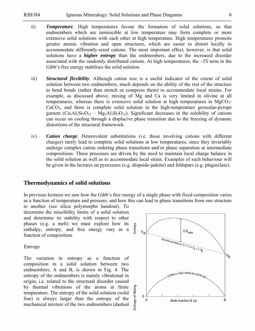
Thermodynamics of solid solutions In previous lectures we saw how the Gibb’s free energy of a single phase with fixed composition varies as a function of temperature and pressure, and how this can lead to phase transitions from one structure to another (see silica polymorphs handout). To determine the miscibility limits of a solid solution and determine its stability with respect to other phases (e.g. a melt) we must explore how its enthalpy, entropy, and free energy vary as a function of composition. Entropy The variation in entropy as a function of composition in a solid solution between two endmembers, A and B, is shown in Fig. 4. The entropy of the endmembers is mainly vibrational in origin, i.e. related to the structural disorder caused by thermal vibrations of the atoms at finite temperature. The entropy of the solid solution (solid line) is always larger than the entropy of the mechanical mixture of the two endmembers (dashed

RJH/H4 Igneous Mineralogy: Solid Solutions and Phase Diagrams 7

line). The excess entropy is called the entropy of mixing (∆Smix) and is predominantly configurational in origin, i.e. it is associated with the large number of energetically-equivalent ways of arranging cations on the available lattice sites. The configurational entropy is strictly defined as:

S = k ln w (1) where k is Boltzmann’s constant and w is the number of degenerate cation configurations. If we consider mixing NA A atoms and NB B atoms on N lattice sites at random, then the number of different configurations of A and B cations is given by:

w =N!

NA!NB!=

N!(xAN)!(xBN)!

(2)

where xA and xB are the mole fractions of A and B. Substituting Eqn. 2 into Eqn. 1 and using Stirling’s approximation (ln N! = N ln N – N, when N is very large), we obtain: S = - Nk (xA ln xA + xB ln xB) (3) If N is taken to be equal to Avagadro’s number then S = - R (xA ln xA + xB ln xB) per mole of sites. In olivine, for example, there are two M sites per formula unit (M1 and M2). If we assume that Mg and Fe2+ mix randomly over both M1 and M2, then the (configurational) entropy of mixing would be - 2R (xMg ln xMg + xFe ln xFe) per mole of M2SiO4. This function is plotted at the bottom of Fig. 4. Enthalpy The variation in enthalpy as a function of composition is shown in Fig. 5. As before, we define the excess enthalpy relative to a mechanical mixture of the two endmembers as the enthalpy of mixing (∆Hmix). Unlike the entropy term, ∆Hmix can be either positive or negative. If ∆Hmix = 0, the solid solution is said to be ideal. If ∆Hmix ≠ 0, the solid solution is said to be non-ideal. An ideal solid solution implies that the substituting cations are very similar (i.e. same charge, similar size, similar bonding characteristics). Solid solutions involving Mg and Fe2+ (e.g. forsterite-fayalite) are often very close to ideal.

Fig. 5

Fig. 4

RJH/H4 Igneous Mineralogy: Solid Solutions and Phase Diagrams 8

The mathematical form of the enthalpy of mixing can be derived using a simple model, assuming the energy of the solid solution arises only from the interaction between nearest-neighbour pairs. Suppose that the coordination number of the lattice sites on which mixing occurs is z. If the total number of sites is N, then the total number of nearest neighbour bonds is 1/2Nz (the number of bonds is half the number of sites). The energy associated with A-A, B-B, and A-B nearest neighbour pairs is WAA, WBB, and WAB, respectively. If cations are mixed randomly, then the probability of A-A, B-B, and A-B neighbours is xA

2, xB2, and

2xAxB, respectively. The total enthalpy of the solid solution is then:

Fig. 6

H = 1/2 Nz (xA

2 WAA + xB2 WBB

+ 2xAxB WAB) (4)

which rearranges to: H = 1/2 Nz (xA WAA + xB WBB) + 1/2 Nz xAxB [2WAB - WAA -WBB] (5) The fist term in Eqn. 5 is the enthalpy of the mechanical mixture. The second term is therefore the enthalpy of mixing:

∆Hmix = 1/2 Nz xAxB [2WAB - WAA - WBB] = 1/2 Nz xAxB W (6) where W is referred to as the regular solution interaction parameter. The sign of W determines the sign of the enthalpy of mixing. If it is energetically more favourable to have A-A and B-B neighbours rather than A-B neighbours, then W is positive and the solid solution will attempt to maximise the number of A-A and B-B neighbours by unmixing into A-rich and B-rich regions (Fig. 6). This processes is referred to as exsolution. If it is energetically more favourable to have A-B neighbours rather than A-A and B-B neighbours, then W is negative and the solid solution will attempt to maximise the number of A-B neighbours by forming an ordered compound (Fig. 6). This process is referred to as cation ordering. If the ordering is associated with a change in symmetry it is referred to as a cation ordering phase transition.

RJH/H4 Igneous Mineralogy: Solid Solutions and Phase Diagrams 9

Free energy The free energy of mixing is defined as:

∆Gmix = ∆Hmix - T∆Smix (7) We explore now the variation in free energy vs. composition and temperature for three cases: i) Ideal solid solution (∆Hmix = 0) Here ∆Gmix = -T∆Smix. Since ∆Smix is always positive, ∆Gmix is always negative. The free energy varies as a function of composition as shown in Fig. 7. The dashed line construction demonstrates that at any composition, the free energy of the single-phase solid solution P is lower than the combined free energy of any mixture of two phases Q and R. The solid solution is stable as a single phase with disordered cation distribution at all compositions and all temperatures. ii) Non-ideal solid solution (∆Hmix > 0) Here the variation in free energy as a function of composition and temperature is more complex due to competition between the positive ∆Hmix term and the negative -T∆Smix term (Fig. 8). At high temperature the -T∆Smix term is dominant, and the free energy curve resembles that of the ideal solid solution. At this temperature the solid solution is stable over the whole range in composition. As the temperature is decreased, the ∆Hmix term and the -T∆Smix term become similar in magnitude and the resulting free energy curve shows two minima and a central maximum. To determine the equilibrium state of the solid solution we first draw the ‘common tangent’, which is a single line tangential to the free energy curve at at least two points (dashed line in Fig. 8). The common tangent touches the free energy curve at Q and R. For bulk compositions between Q and R (e.g. point P in Fig. 8), the free energy of the single-phase solid solution is higher than the free energy of a mixture of Q and R. At equilibrium, the system will minimise its free energy by exsolving to two phases with compositions Q and R. For bulk compositions outside Q and R, the free

Fig. 7

Fig. 8

RJH/H4 Igneous Mineralogy: Solid Solutions and Phase Diagrams 10

energy of any mixture of two phases is greater than the free energy of the single-phase solid solution, and the solid solution remains stable as a single phase. At lower temperature, the position of the minima in free energy move towards the endmembers (points Q’ and R’ in Fig. 8). If we plot the locus of the equilibrium compositions as a function of temperature, we obtain the binary phase diagram for the system (Fig 9). The phase diagram defines the compositions of phases in equilibrium with each other at a given temperature. In this case a miscibility gap or solvus develops at low temperature. At temperatures and compositions outside the solvus, the single-phase solid solution is stable. Inside the solvus, a solid solution P with composition C0 exsolves into an intergrowth of phase Q and R with compositions C1 and C2, respectively.

Fig. 9

The proportions of the two phases in the intergrowth are given by the lever rule. To calculate the proportion of a phase you simply divide the difference between the bulk composition (C0) and the composition of the other phase (either C1 or C2) by the difference between the composition of the two phases (C2 – C1). Hence, the proportion of phase Q is given by the ratio (C2 – C0) / (C2 – C1) and the proportion of phase R is given by the ratio (C0 – C1) / (C2 – C1). iii) Non-ideal solid solution (∆Hmix < 0) Here the change in free energy relative to the ideal case is more subtle (Fig. 10). There is a strong driving force for cation ordering in the centre of the solid solution, where the ratio of A:B cations is 1:1. The fully-ordered phase has zero configurational entropy, because there is just one way to arrange the atoms (two if you include the equivalent anti-ordered state). However, it has a low enthalpy due to the energetically-favourable arrangement of cations. This stabilises the ordered phase at low temperature, where the –T∆Smix term in

Fig. 10

RJH/H4 Igneous Mineralogy: Solid Solutions and Phase Diagrams 11

the free energy is less important. The fully disordered solid solution has a high configurational entropy, which stabilises it at high temperature. There is a phase transition from the ordered phase to the disordered phase at a critical transition temperature (Tc). The phase diagram for a 2nd-order cation ordering phase transition simply shows a transition from a single-phase disordered solid solution to a single-phase ordered solid solution at each composition, with the transition temperature varying parabolically as a function of composition (Fig. 11). Crystallisation of an ideal solid solution from a melt Here we consider the solidification of an ideal solid solution from a melt. The free energy of mixing is similar in both phases, since this is dominated by the same configurational entropy of mixing term (Eqn. 3). However, the relative positions of the solid and melt free energy curves change with temperature, since the absolute entropy of the melt is greater than the solid (remember that dG/dT = -S; see silica polymorph handout).

Fig. 11

Fig. 12

RJH/H4 Igneous Mineralogy: Solid Solutions and Phase Diagrams 12

The sequence of events on cooling is as follows:

i) T = T1. The free energy of the melt is lower than that of the solid solution at all compositions. Therefore the melt is the stable phase at all compositions.

ii) T = TA. The free energy of the solid endmember A is equal to the free energy of molten A.

This corresponds to the cystallisation temperature of the A endmember.

iii) T = T2. The free energies of the solid solution and melt intersect. Using the common tangent construction we see that from 0 to Csolid, the single-phase solid solution is stable. Between Csolid and Cmelt the system consists of a solid phase with composition Csolid in equilibrium with a liquid phase of composition Cmelt. Beyond Cmelt, the single-phase melt is stable.

iv) T = T3. Compositions of Csolid and Cmelt move from left to right with decreasing temperature.

v) T = TB. The free energy of the solid endmember B is equal to the free energy of molten B.

This corresponds to the crystallisation temperature of the B endmember.

vi) T = T4. The free energy of the solid solution is lower than that of the melt at all compositions. Therefore the solid solution is the stable phase at all compositions.

As an example, the phase diagram for the forsterite-fayalite solid solution is shown in Fig. 13. The phase diagram consists of a simple loop formed from two curves. The top curve is called the liquidus and the bottom is called the solidus. These define the compositions of solid and liquid phases in equilibrium with each other. The stages of crystallisation for a melt of composition x0 are as follows: i) Above the liquidus the single-phase melt is stable. ii) On entering the loop, the first

solid to form has composition x1. This is in equilibrium with melt of composition y1 ( = x0). At this stage, the system consists of 100% melt and 0% solid (use the lever rule!).

iii) Halfway through the loop, the

composition of the solid forming has moved to x2 and the composition of the melt in equilibrium with this solid has moved to y2 (note that slow cooling is required for the solid and melt to remain in equilibrium with each other. If cooling is too fast then the crystals forming will be chemically zoned). We now have roughly equal proportions of solid and melt.

Fig. 13

RJH/H4 Igneous Mineralogy: Solid Solutions and Phase Diagrams 13

iv) When we reach the solidus, the composition of the solid has reached x3 ( = x0) and the melt in equilibrium with it has composition y3. Now the lever rule shows that the system consists of 100% solid and 0% melt. If cooling was slow then we have obtained a single-phase homogeneous solid solution with bulk composition equal to the bulk composition of the original melt.

A note on fractional crystallisation Above we have described the process of equilibrium crystallisation, where the cooling is slow and the solid and melt phases are allowed to remain in equilibrium with each other at all times. Later in the course you will come across the process of fractional crystallisation, where the solid phase is removed from the melt as soon as it forms. This process occurs, for example, due to the gravitational settling of crystals to the bottom of a magma chamber, where they are prevented from further reaction with the residual melt. It is clear from Fig. 13 that the composition of the first crystals to form from a melt are chemically enriched in one component. Conversely, the residual melt is depleted in that component. As more crystals form and are removed from the melt, the bulk composition of the melt evolves to compositions far removed from the original bulk composition. Other types of melting loops If the curvature of the G-x curves for solid solution and melt are very different, then melting loops of the form shown in Fig. 14 may result. In the first case, the curvature of the melt G-x curve is greater than that of the solid solution, and both liquidus and solidus show a thermal minimum, with melting loops on either side. At the minimum, melt with intermediate composition crystallises directly into a solid solution, without going through a two-phase region. If the curvature of the solid solution G-x curve is greater than that of the melt, then a thermal maximum arises and the loops are inverted.

Fig. 14

Crystallisation where two endmembers have limited solid solution So far we have considered a simple system showing complete solid solution either at all temperatures or at high temperatures. For this to be the case, both endmembers must have the same crystal structure and symmetry (as in the case of forsterite-fayalite). We now explore the phase diagrams of systems where the two endmembers have different structures and show only limited solid solution.

RJH/H4 Igneous Mineralogy: Solid Solutions and Phase Diagrams 14

Because the two endmembers have different structures, they are represented by separate free energy curves (labelled α and β in Fig. 15). Because the degree of solid solution permitted in each endmember is limited, the curvature of the free energy curves is much larger than depicted so far. i) T = T1. Melt is stable at all

compositions. ii) T = TA. Crystallisation

temperature of pure A. iii) T = TB. Crystallisation

temperature of pure B. Two-phase region in A-rich compositions.

iv) T = TE. At one particular

temperature, all three phases lie on the same common tangent (i.e. are in equilibrium with each other). This is called the eutectic temperature.

v) T = T2. Below the eutectic

temperature the melt is no longer stable at any composition, and there is a large central miscibility gap.

The resulting phase diagram can be interpreted as the intersection of a melting loop of the form shown in Fig. 14 with a simple solvus of the form shown in Fig. 9. The eutectic point defines the composition of the melt in equilibrium with two solids at the eutectic temperature. Fig. 15

In the limit that no solid solution is tolerated by endmembers A and B, the phase diagram appears as in Fig. 16. Fig. 16

RJH/H4 Igneous Mineralogy: Solid Solutions and Phase Diagrams 15

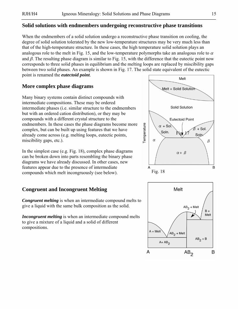
Solid solutions with endmembers undergoing reconstructive phase transitions When the endmembers of a solid solution undergo a reconstructive phase transition on cooling, the degree of solid solution tolerated by the new low-temperature structures may be very much less than that of the high-temperature structure. In these cases, the high temperature solid solution plays an analogous role to the melt in Fig. 15, and the low-temperature polymorphs take an analogous role to α and β. The resulting phase diagram is similar to Fig. 15, with the difference that the eutectic point now corresponds to three solid phases in equilibrium and the melting loops are replaced by miscibility gaps between two solid phases. An example is shown in Fig. 17. The solid state equivalent of the eutectic point is renamed the eutectoid point.

Fig. 18

Fig. 17

More complex phase diagrams Many binary systems contain distinct compounds with intermediate compositions. These may be ordered intermediate phases (i.e. similar structure to the endmembers but with an ordered cation distribution), or they may be compounds with a different crystal structure to the endmembers. In these cases the phase diagrams become more complex, but can be built up using features that we have already come across (e.g. melting loops, eutectic points, miscibility gaps, etc.). In the simplest case (e.g. Fig. 18), complex phase diagrams can be broken down into parts resembling the binary phase diagrams we have already discussed. In other cases, new features appear due to the presence of intermediate compounds which melt incongruously (see below). Congruent and Incongruent Melting Congruent melting is when an intermediate compound melts to give a liquid with the same bulk composition as the solid. Incongruent melting is when an intermediate compound melts to give a mixture of a liquid and a solid of different compositions.

RJH/H4 Igneous Mineralogy: Solid Solutions and Phase Diagrams 16

An example of a congruently melting intermediate compound is shown in Fig. 18 (AB2). This compound represents a thermal maximum in the phase diagram, i.e. melts of bulk composition to the left of AB2 will ultimately crystallise to a mixture of A + AB2 (and could never produce any B) whereas melts with bulk composition to the right of AB2 will ultimately crystallise to AB2 + B (and could never produce any A). The sequence of G-x curves leading to incongruent melting is shown in Fig. 19, along with the resulting phase diagram. In this case an intermediate compound AB melts to give a mixture of B-rich melt and pure A. The reaction occurs at a peritectic temperature, at which A, AB, and the melt are in equilibrium with each other (i.e. all lie on the same common tangent). The composition of the liquid at the peritectic temperature defines the peritectic point.

9

Note that the intermediate compound in this case dcompositional evolution of a melt. Under equilibrileft of AB would ultimately crystallise a mixture ovia fractional crystallisation to yield bulk composipure B at a lower temperature.

Fi

Fig. 1

oes not represent a thermal barrier to the um conditions, a melt with bulk composition to the f A + AB (i.e. no B). However the melt could evolve tions to the right of AB. This could then produce

g. 20

RJH/H4 Igneous Mineralogy: Solid Solutions and Phase Diagrams 17

An example of an incongruently melting intermediate compound is the pyroxene mineral enstatite (MgSiO3), within the binary system between forsterite (Mg2SiO4) and silica (SiO2) (Fig. 20). At atmospheric pressure pure enstatite melts incongruously to yield a mixture of forsterite + melt. The phase relations change dramatically at higher pressures (note the disappearance of the liquid miscibity gap in SiO2-rich melts and the gradual replacement of the low pressure silica polymorphs tridymite and cristobalite by quartz). Most important, however, is that enstatite melts congruously at higher pressure, creating a thermal barrier between forsterite and quartz. These two minerals are therefore incompatible with each other at these conditions – i.e. a melt of any composition could not be made to precipitate both forsterite and quartz. Geological occurrence and significance of olivine Igneous Rocks Mg-rich (forsterite-rich) olivines with compositions from about Fo60 to Fo86 commonly occur in relatively low silica plutonic (gabbro, diorite, etc.) and volcanic (basalt, basaltic andesite, andesite) igneous rocks. Within these rock groups, the forsterite content of the olivine generally decreases (i.e. the olivine becomes more iron rich) and the abundance of the olivine decreases as the silica content of the rock increases. For example, basalts (about 50 wt.% silica) typically have abundant olivine that ranges in composition from about Fo86 to Fo75, while andesites (about 55-62 wt.% silica) typically have only a few percent at most of Fo75 to Fo60 olivines. In these relatively low silica rocks, olivine typically coexists with minerals such as: plagioclase, clinopyroxene, orthopyroxene, spinels, ilmenite and occasionally amphibole. Mg-rich olivines never coexist with quartz at equilibrium. Metamorphic Rocks Olivine also occurs in metamorphic rocks. One common occurrence is in marbles (metamorphosed limestones), where nearly pure forsterite or monticellite (CaMgSiO4) are sometimes found coexisting with diopside, calcite, grossularite garnet, tremolite and epidote group minerals. Olivine in the Mantle

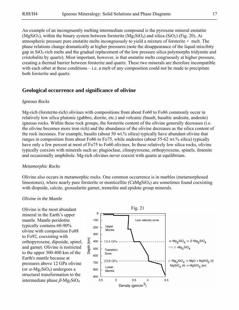
Fig. 21 Olivine is the most abundant mineral in the Earth’s upper mantle. Mantle peridotite typically contains 60-90% olvine with composition Fo88 to Fo92, coexisting with orthopyroxene, diposide, spinel, and garnet. Olivine is restricted to the upper 300-400 km of the Earth's mantle because at pressures above 12 GPa olivine (or α-Mg2SiO4) undergoes a structural transformation to the intermediate phase β-Mg2SiO4

RJH/H4 Igneous Mineralogy: Solid Solutions and Phase Diagrams 18

(wadsleyite) and then to cubic spinel structure γ-Mg2SiO4 (ringwoodite). These transformations are accompanied by a significant increase in density, which also results in an increase in the propagation velocities of seismic waves (Fig. 21). The olivine to β-phase transition at 400 km marks the boundary between the upper mantle and the transition zone. The transition pressure is sensitive to the Fe-content of the olivine, which may be significant in determining the sharpness of the transitions in the mantle (Fig. 22).