NATIONAL OPEN UNIVERSITY OF NIGERIA SCHOOL OF …nouedu.net/sites/default/files/2017-03/MTH103.pdf · · 2017-03-09"Download for free at the National Open University of Nigeria

NATIONAL OPEN UNIVERSITY OF NIGERIA

SCHOOL OF SCIENCE AND TECHNOLOGY

COURSE CODE: MTH 103

COURSE TITLE: ELEMENTARY MATHEMATICS III

COURSE GUIDE

Course Developer/Writers Dr. Ajibola. S.O

National Open University of Nigeria

Lagos, Nigeria,

and

Dr. Peter Ogedebe

Base University, Abuja

Content Editor { Prof. U.A Osisiogu. }

{ Faculty of Physical Sciences }

{Department of Mathematics,}

{ Eboyin State University }

{ Eboyin, Nigeria}

Course Coordinators Dr. Disu Babatunde

and

Babatunde Osho.j

School of Science and Technology


Lagos, Nigeria,


Headquarters

14/16 Ahmadu Bello Way

Victoria Island

Lagos

Published in 2015 by the National Open University of Nigeria, 14/16 Ahmadu Bello Way, Victoria

Island, Lagos, Nigeria

© National Open University of Nigeria 2015

This publication is made available in Open Access under the Attribution-ShareAlike4.0 (CC-BY-SA

4.0) license (http://creativecommons.org/licenses/by-sa/4.0/). By using the content of this

publication, the users accept to be bound by the terms of use of the National Open University of

Nigeria Open Educational Resources Repository: http://www.oer.nou.edu.ng

The designations employed and the presentation of material throughout this publication do not

imply the expression of any opinion whatsoever on the part of National Open University of Nigeria

concerning the legal status of any country, territory, city or area or of its authorities, or concerning

the delimitation of its frontiers or boundaries. The ideas and opinions expressed in this

publication are those of the authors; they are not necessarily those of National Open University of

Nigeria and do not commit the Organization.

How to Reuse and Attribute this content

Under this license, any user of this textbook or the textbook contents herein must provide proper

attribution as follows: “First produced by the National Open University of Nigeria” and include the

NOUN Logo and the cover of the publication.

http://www.oer.nou.edu.ng/

If you use this course material as a bibliographic reference, then you should cite it as follows:

“Course code: Course Title, National Open University of Nigeria, 2014 at

http://www.nou.edu.ng/index.htm#

If you redistribute this textbook in a print format, in whole or part, then you must include on

every physical page the following attribution:

"Download for free at the National Open University of Nigeria Open Educational Resources

Repository at http://www.nou.edu.ng/index.htm#).

If you electronically redistribute part of this textbook, in whole or part, then you must retain in

every digital format page view (including but not limited to EPUB, PDF, and HTML) the

following attribution:

"Download for free, National Open University of Nigeria Open Educational Resources

Repository athttp://www.nou.edu.ng/index.htm#)

http://www.nou.edu.ng/index.htm



Course Guide

Course Code: MTH 103

Course Title: ELEMENTARY MATHEMATICS III

Introduction

MTH 103 - Elemetary Mathematics III is designed to teach you how mathematics could be used in solving problems in the contemporary Scientific world. Therefore, the course is structured to expose you to the

skills required in other to attain a level of proficiency in Sciences,technology and Engineering Professions.

What you will learn in this Course

You will be taught the basis of mathematics required in solving

s c ie n t i f i c problems.

Course Aim

There are eleven study units in the course and each unit has its objectives.

You should read the objectives of each unit and bear them in mind as

you go through the unit. In addition to the objectives of each unit, the

overall aims of this course include:

(i) To introduce you to the words and concepts in Elementary mathematics

(ii) To familiarize you with the peculiar characteristics in Elementary mathematics.

(iii) To expose you to the need for and the demands of mathematics in

the Science world.

(iv) To prepare you for the contemporary Science world.

Course Objectives

The objectives of this course are:

To inculcate appropriate mathematical skills required in

Science and Engineering.

Educate learners on how to use mathematical Techniques in

solving real life problems.

Educate the learners on how to integrate mathematical models in

Sciences, technology and Engineering.

Working through this Course

{ You have to work through all the study units in the course. There are two modules and ten study units in all.

Course Materials

Major components of the course

are:

1. Course

Guide

2. Study

Units

3.

Textbooks

4. CDs

5. Assignments File

6. Presentation Schedule

Study Units

The breakdown of the four modules and eleven study units are as follows:

The breakdown of the four modules and eleven study units are as follows:

Vectors 1.1 Introduction . . . . . . . . . . . . . . . . . . . . . . . 8 1.2 Objectives . . . . . . . . . . . . . . . . . . . . . . . . 8 1.3 Main Contents . . . . . . . . . . . . . . . . . . . . . 9 1.3.1 Physical Quantities . . . . . . . . . . . . . . . . 9 1.3.2 Geometrical Representation of Vectors in 1- 3 dimensions . . . . . . . . . . . . . . . . . . . . . . . . . 9 1.3.3 Two Equal Vectors . . . . . . . . . . . . . . . . 11 1.3.4 Types of Vectors . . . . . . . . . . . . . . . . . . 12 1.4 Conclusion . . . . . . . . . . . . . . . . . . . . . . . . 12 1.5 Summary . . . . . . . . . . . . . . . . . . . . . . . . . 12 1.6 Exercise . . . . . . . . . . . . . . . . . . . . . . . . . . 13 1.7 References . . . . . . . . . . . . . . . . . . . . . . . . 13 2 Additions of Vectors 2.1 Introduction . . . . . . . . . . . . . . . . . . . . . . . . 14 2.2 Main Content . . . . . . . . . . . . . . . . . . . . . . . 15 2.2.1 Sum of a Number of Vectors . . . . . . . . . 16 2.3 Conclusion . . . . . . . . . . . . . . . . . . . . . . . . . 17 2.4 Summary . . . . . . . . . . . . . . . . . . . . . . . . . . 17 2.5 Exercises . . . . . . . . . . . . . . . . . . . . . . . . . . 18 2.6 References . . . . . . . . . . . . . . . . . . . . . . . . . 18 3 Components of a Given Vector 3.1 Introduction . . . . . . . . . . . . . . . . . . . . . . . . . 19 3.2 Objectives . . . . . . . . . . . . . . . . . . . . . . . . . . 19 3.3 Main Content . . . . . . . . . . . . . . . . . . . . . . . . 20 3.3.1 Component of an given vector. . . . . . . . . . 20 3.4 Conclusion . . . . . . . . . . . . . . . . . . . . . . . . . . 23 3.5 Summary . . . . . . . . . . . . . . . . . . . . . . . . . . . 23 3.6 Exercises . . . . . . . . . . . . . . . . . . . . . . . . . . . 24 3.7 References . . . . . . . . . . . . . . . . . . . . . . . . . . 24 4 Components of a Vector in terms of Unit vectors and Vectors in Space 4.1 Introduction . . . . . . . . . . . . . . . . . . . . . . . . . . 25 4.2 Objectives . . . . . . . . . . . . . . . . . . . . . . . . . . . 25 4.3 Main Contents . . . . . . . . . . . . . . . . . . . . . . . . 26 4.3.1 Components of a vector in terms of Unit Vectors . . . . . . . . . . . . . . . . . . . . . . . . . . . . . . . . 26 4.3.2 Vectors in Space . . . . . . . . . . . . . . . . . . . . 28 4.4 Conclusion . . . . . . . . . . . . . . . . . . . . . . . . . . 30 4.5 Summary . . . . . . . . . . . . . . . . . . . . . . . . . . . . 30 4.6 Exercise . . . . . . . . . . . . . . . . . . . . . . . . . . . . 30 4.7 References . . . . . . . . . . . . . . . . . . . . . . . . . . 31 5 Direction Cosines 5.1 Introduction . . . . . . . . . . . . . . . . . . . . . . . . . . 32 5.2 Objectives . . . . . . . . . . . . . . . . . . . . . . . . . . . 32 5.3 Main Content . . . . . . . . . . . . . . . . . . . . . . . . . 33 5.3.1 Direction Cosines . . . . . . . . . . . . . . . . . . . . 33 5.4 Summary . . . . . . . . . . . . . . . . . . . . . . . . . . . . 34 5.5 Exercises . . . . . . . . . . . . . . . . . . . . . . . . . . . . 35 5.6 References . . . . . . . . . . . . . . . . . . . . . . . . . . 35

6 Scalar Product of two vectors 6.1 Introduction . . . . . . . . . . . . . . . . . . . . . . . . . . 36 6.2 Objectives . . . . . . . . . . . . . . . . . . . . . . . . . . . 36 6.3 Main Content . . . . . . . . . . . . . . . . . . . . . . . . . 37 6.3.1 Scalar product of two vectors . . . . . . . . . . . 37 6.3.2 Expressing Scalar Product Of Two Vectors In Terms Of The Unit Vector I, j, k. . . . . . . . . . . . . 40 6.4 Conclusion . . . . . . . . . . . . . . . . . . . . . . . . . . . 41 6.5 Summary . . . . . . . . . . . . . . . . . . . . . . . . . . . . . 41 6.6 Exercises . . . . . . . . . . . . . . . . . . . . . . . . . . . . . 41 6.7 References . . . . . . . . . . . . . . . . . . . . . . . . . . . 42 7 Vector Product of Two Vectors 7.1 Introduction . . . . . . . . . . . . . . . . . . . . . . . . . . 43 7.2 Objectives . . . . . . . . . . . . . . . . . . . . . . . . . . . . 43 7.3 Main Content . . . . . . . . . . . . . . . . . . . . . . . . . . 44 7.3.1 Vector Product of Two Vectors . . . . . . . . . . . 44 7.3.2 Expressing Vector Product of two Vectors in Terms of the Unit Vectors i,j and k. . . . . . . . . . . . . . . . . . . . . . . . . . . . 46 7.4 Conclusion . . . . . . . . . . . . . . . . . . . . . . . . . . . . . 47 7.5 Summary . . . . . . . . . . . . . . . . . . . . . . . . . . . . . . 47 7.6 Exercises . . . . . . . . . . . . . . . . . . . . . . . . . . . . . . 48 7.7 References . . . . . . . . . . . . . . . . . . . . . . . . . . . . . 48 8 Loci 8.1 Introduction . . . . . . . . . . . . . . . . . . . . . . . . . . . . . 49 8.2 Objectives . . . . . . . . . . . . . . . . . . . . . . . . . . . . . . 50 8.3 Main Content . . . . . . . . . . . . . . . . . . . . . . . . . . . 50 8.3.1 Straight Line . . . . . . . . . . . . . . . . . . . . . . . . . . 50 8.3.2 Cartesian Coordinates . . . . . . . . . . . . . . . . . . 50 8.3.3 Distance between two Points and Midpoint of two Points . . . . . . . . . . . . . . . . . . . . . . . . . . . . . . 51 8.3.4 Gradient (gradient, angle of slope, and equation of a straight line). . . . . . . . . . . . . . . . . . . . . . . . 54 8.3.5 Angle Between two Lines . . . . . . . . . . . . . . . . 60 8.4 Conclusion . . . . . . . . . . . . . . . . . . . . . . . . . . . . . 64 8.5 Summary . . . . . . . . . . . . . . . . . . . . . . . . . . . . . . 64 8.6 Exercises . . . . . . . . . . . . . . . . . . . . . . . . . . . . . . 65 8.7 References . . . . . . . . . . . . . . . . . . . . . . . . . . . . 66 9 Coordinate Geometry (Circle) 9.1 Introduction . . . . . . . . . . . . . . . . . . . . . . . . . . . . 67 9.2 Objectives . . . . . . . . . . . . . . . . . . . . . . . . . . . . . 67 9.3 Main Content . . . . . . . . . . . . . . . . . . . . . . . . . . . 68 9.3.1 Equation of a circle . . . . . . . . . . . . . . . . . . . . . 68 9.3.2 Parametric Equation of a Circle . . . . . . . . . . . 74 9.3.3 Points Outside and Inside a Circle . . . . . . . . . 75 9.3.4 Touching Circles . . . . . . . . . . . . . . . . . . . . . . . 76 9.3.5 Tangents to a Circle . . . . . . . . . . . . . . . . . . . . 78 9.4 Conclusion . . . . . . . . . . . . . . . . . . . . . . . . . . . . . 79 9.5 Summary . . . . . . . . . . . . . . . . . . . . . . . . . . . . . . 79 9.6 Exercises . . . . . . . . . . . . . . . . . . . . . . . . . . . . . . 80 9.7 References . . . . . . . . . . . . . . . . . . . . . . . . . . . . . 81

10 Parabola 10.1 Introduction . . . . . . . . . . . . . . . . . . . . . . . . . . . . 82 10.2 Objectives . . . . . . . . . . . . . . . . . . . . . . . . . . . . . 82 10.3 Main Content . . . . . . . . . . . . . . . . . . . . . . . . . . . 83 10.3.1 De_nition of Parabola . . . . . . . . . . . . . . . . . . . 83 10.3.2 The formula for a parabola vertical axis. . . . . . .84 10.3.3 Parabola with horizontal axis. . . . . . . . . . . . . . . 86 10.3.4 Shifting the vertex of a parabola from the origin. . . . . . . . . . . . . . . . . . . . . . . . . . . . . . . . . . . . . . . 88 10.4 Conclusion . . . . . . . . . . . . . . . . . . . . . . . . . . . . . . 91 10.5 Summary . . . . . . . . . . . . . . . . . . . . . . . . . . . . . . . 92 10.6 References . . . . . . . . . . . . . . . . . . . . . . . . . . . . . . 92 11 Ellipse and Hyperbola 11.1 Introduction . . . . . . . . . . . . . . . . . . . . . . . . . . . . . . 93 11.2 Objectives . . . . . . . . . . . . . . . . . . . . . . . . . . . . . . . 93 11.3 Main Content . . . . . . . . . . . . . . . . . . . . . . . . . . . . . 94 11.3.1 Ellipse . . . . . . . . . . . . . . . . . . . . . . . . . . . . . . . . . 94 11.3.2 Hyperbola . . . . . . . . . . . . . . . . . . . . . . . . . . . . . . 98 11.4 Conclusion . . . . . . . . . . . . . . . . . . . . . . . . . . . . . . . 102 11.5 Summary . . . . . . . . . . . . . . . . . . . . . . . . . . . . . . . . 102 11.6 Exercises . . . . . . . . . . . . . . . . . . . . . . . . . . . . . . . . 103 11.7 References . . . . . . . . . . . . . . . . . . . . . . . . . . . . . . . 104

Recommended Texts

o Larson Edwards Calculus: An Applied Approach. Sixth Edition.

o Blitzer. Algebra and Trigonometry Custom. 4th Edition

o K.A Stroud. Engineering Mathematics. 5th Edition

o Pure Mathematics for Advanced Level By B.D Bunday H Mulholland1970.

o Godman and J.F Talbert. Additional Mathematics

Assignment File

{ In this file, you will find all the details of the work you must submit to your

tutor for marking. The marks you obtain from these assignments will count

towards the final mark you obtain for this course. Further information on

assignments will be found in the Assignment File itself and later in this Course

Guide in the section on assessment.

Presentation Schedule

The Presentation Schedule included in your course materials gives you the

important dates for the completion of tutor-marked assignments and attending

tutorials. Remember, you are required to submit all your assignments by the

due date. You should guard against falling behind in your work.

Assessment

Your assessment will be based on tutor-marked assignments (TMAs) and a

final examination which you will write at the end of the course.

Exercises TMAS

{ Every unit contains at least one or two assignments. You are advised to work

through all the assignments and submit them for assessment. Your tutor will

assess the assignments and select four which will constitute the 30% of your

final grade. The tutor-marked assignments may be presented to you in a

separate file. Just know that for every unit there are some tutor-marked

assignments for you. It is important you do them and submit for assessment. }

Final Examination and Grading

{ At the end of the course, you will write a final examination which will

constitute 70% of your final grade. In the examination which shall last for two

hours, you will be requested to answer three questions out of at least five

questions.

Course marking Scheme

This table shows how the actual course marking as it is broken down.

Assessment Marks

Assignments Four assignments, Best three marks of

the four count at 30% of course marks

Final Examination 70% of overall course marks

Total

100% of course marks

How to Get the Most from This Course

In distance learning, the study units replace the university lecture. This is one

of the great advantages of distance learning; you can read and work through

specially designed study materials at your own pace, and at a time and place

that suits you best. Think of it as reading the lecture instead of listening to the

lecturer. In the same way a lecturer might give you some reading to do, the

study units tell you when to read, and which are your text materials or set

books. You are provided exercises to do at appropriate points, just as a lecturer

might give you an in-class exercise. Each of the study units follows a common

format. The first item is an introduction to the subject matter of the unit, and

how a particular unit is integrated with the other units and the course as a

whole. Next to this is a set of learning objectives. These objectives let you

know what you should be able to do by the time you have completed the unit.

These learning objectives are meant to guide your study. The moment a unit is

finished, you must go back and check whether you have achieved the

objectives. If this is made a habit, then you will significantly improve your

chances of passing the course. The main body of the unit guides you through

the required reading from other sources. This will usually be either from your

set books or from a Reading section. The following is a practical strategy for

working through the course. If you run into any trouble, telephone your tutor.

Remember that your tutor’s job is to help you. When you need assistance, do

not hesitate to call and ask your tutor to provide it.

In addition do the following:

1. Read this Course Guide thoroughly, it is your first assignment.

2. Organise a Study Schedule. Design a Course Overview ‟ to guide you

through the Course”. Note the time you are expected to spend on each unit and

how the assignments relate to the units. Important information, e.g. details of

your tutorials, and the date of the first day of the Semester is available from the

study centre. You need to gather all the information into one place, such as

your diary or a wall calendar. Whatever method you choose to use, you should

decide on and write in your own dates and schedule of work for each unit.

3. Once you have created your own study schedule, do everything to stay

faithful to it. The major reason that students fail is that they get behind with

their course work. If you get into difficulties with your schedule, please, let

your tutor know before it is too late for help.

4. Turn to Unit 1, and read the introduction and the objectives for the unit.

5. Assemble the study materials. You will need your set books and the unit you are

studying at any point in time.

6. Work through the unit. As you work through the unit, you will know what

sources to consult for further information.

7. Keep in touch with your study centre. Up-to-date course information will be

continuously available there.

8. Well before the relevant due dates (about 4 weeks before due dates), keep in

mind that you will learn a lot by doing the assignment carefully. They have

been designed to help you meet the objectives of the course and, therefore, will

help you pass the examination. Submit all assignments not later than the due

date.

9. Review the objectives for each study unit to confirm that you have achieved

them. If you feel unsure about any of the objectives, review the study materials or

consult your tutor.

10. When you are confident that you have achieved a unit’s objectives, you can

start on the next unit. Proceed unit by unit through the course and try to pace

your study so that you keep yourself on schedule.

11. When you have submitted an assignment to your tutor for marking, do not

wait for its return before starting on the next unit. Keep to your schedule.

When the Assignment is returned, pay particular attention to your tutor’s

comments, both on the tutor-marked assignment form and also the written

comments on the ordinary assignments.

12. After completing the last unit, review the course and prepare yourself for

the final examination. Check that you have achieved the unit objectives (listed at

the beginning of each unit) and the course objectives (listed in the Course

Guide).

Tutors and Tutorials

The dates, times and locations of these tutorials will be made available to you,

together with the name, telephone number and the address of your tutor. Each

assignment will be marked by your tutor. Pay close attention to the comments

your tutor might make on your assignments as these will help in your progress.

Make sure that assignments reach your tutor on or before the due date.

Your tutorials are important therefore try not to skip any. It is an opportunity to

meet your tutor and your fellow students. It is also an opportunity to get the

help of your tutor and discuss any difficulties encountered on your reading.

Summary

This course would train you on the concept of multimedia, production and

utilization of it.

Wish you the best of luck as you read through this course

MAT 103

ELEMENTARY MATHEMATICS III

(VECTORS, GEOMETRY AND DYNAMICS)

Edited By

Prof. U. A. Osisiogu

1

Contents

1 Vectors 8

1.1 Introduction . . . . . . . . . . . . . . . . . . . . . 8

1.2 Objectives . . . . . . . . . . . . . . . . . . . . . . 8

1.3 Main Contents . . . . . . . . . . . . . . . . . . . 9

1.3.1 Physical Quantities: . . . . . . . . . . . . 9

1.3.2 Geometrical Representation of Vectors in 1-

3 dimensions . . . . . . . . . . . . . . . . 9

1.3.3 Two Equal Vectors . . . . . . . . . . . . . 11

1.3.4 Types of Vectors . . . . . . . . . . . . . . 12

1.4 Conclusion . . . . . . . . . . . . . . . . . . . . . . 12

1.5 Summary . . . . . . . . . . . . . . . . . . . . . . 12

1.6 Exercise . . . . . . . . . . . . . . . . . . . . . . . 13

1.7 References . . . . . . . . . . . . . . . . . . . . . . 13

2 Addition of Vectors 14

2

2 CONTENTS

2.1

Introduction . . . . . . . . . . . . .

.

.

.

.

.

.

.

.

14

2.2 Main Content . . . . . . . . . . . . . . . . . . . . 15

2.2.1 Sum of a Number of Vectors . . . . . . . 16

2.3 Conclusion . . . . . . . . . . . . . . . . . . . . . . 17

2.4 Summary . . . . . . . . . . . . . . . . . . . . . . 17

2.5 Exercises . . . . . . . . . . . . . . . . . . . . . . . 18

2.6 References . . . . . . . . . . . . . . . . . . . . . . 18

3 Components of a Given Vector 19

3.1 Introduction . . . . . . . . . . . . . . . . . . . . . 19

3.2 Objectives . . . . . . . . . . . . . . . . . . . . . . 19

3.3 Main Content . . . . . . . . . . . . . . . . . . . . 20

3.3.1 Component of an given vector. . . . . . . . 20

3.4 Conclusion . . . . . . . . . . . . . . . . . . . . . . 23

3.5 Summary . . . . . . . . . . . . . . . . . . . . . . 23

3.6 Exercises . . . . . . . . . . . . . . . . . . . . . . . 24

3.7 References . . . . . . . . . . . . . . . . . . . . . . 24

4 Components of a Vector in terms of Unit vectors

and Vectors in Space 25

4.1 Introduction . . . . . . . . . . . . . . . . . . . . . 25

4.2 Objectives . . . . . . . . . . . . . . . . . . . . . 25

4.3 Main Contents . . . . . . . . . . . . . . . . . . . 26

4.3.1 Components of a vector in terms of Unit

Vectors . . . . . . . . . . . . . . . . . . . . 26

4.3.2 Vectors in Space . . . . . . . . . . . . . . 28

4.4 Conclusion . . . . . . . . . . . . . . . . . . . . . . 30

4.5 Summary . . . . . . . . . . . . . . . . . . . . . . 30

3

3 CONTENTS

4.6

Exercise . . . .

.

.

.

.

.

.

.

.

.

.

.

.

.

.

.

.

.

.

.

30

4.7 References . . . . . . . . . . . . . . . . . . . . . . 31

5 Direction Cosines 32

5.1 Introduction . . . . . . . . . . . . . . . . . . . . . 32

5.2 Objectives . . . . . . . . . . . . . . . . . . . . . . 32

5.3 Main Content . . . . . . . . . . . . . . . . . . . . 33

5.3.1 Direction Cosines . . . . . . . . . . . . . . 33

5.4 Summary . . . . . . . . . . . . . . . . . . . . . . 34

5.5 Exercises . . . . . . . . . . . . . . . . . . . . . . . 35

5.6 References . . . . . . . . . . . . . . . . . . . . . . 35

6 Scalar Product of two vectors 36

6.1 Introduction . . . . . . . . . . . . . . . . . . . . . 36

6.2 Objectives . . . . . . . . . . . . . . . . . . . . . . 36

6.3 Main Content . . . . . . . . . . . . . . . . . . . . 37

6.3.1 Scalar product of two vectors . . . . . . . 37

6.3.2 Expressing Scalar Product Of Two Vectors

In Terms Of The Unit Vector I, j, k. . . . 40

6.4 Conclusion . . . . . . . . . . . . . . . . . . . . . . 41

6.5 Summary . . . . . . . . . . . . . . . . . . . . . . 41

6.6 Exercises . . . . . . . . . . . . . . . . . . . . . . . 41

6.7 References . . . . . . . . . . . . . . . . . . . . . . 42

7 Vector Product of Two Vectors 43

7.1 Introduction . . . . . . . . . . . . . . . . . . . . . 43

7.2 Objectives . . . . . . . . . . . . . . . . . . . . . . 43

7.3 Main Conte nt . . . . . . . . . . . . . . . . . . . . 44

4

4 CONTENTS

7.3.1 Vector Product of Two Vectors . . . . . . 44

7.3.2 Expressing Vector Product of two Vectors

in Terms of the Unit Vectors i,j and k. . . 46

7.4 Conclusion . . . . . . . . . . . . . . . . . . . . . . 47

7.5 Summary . . . . . . . . . . . . . . . . . . . . . . 47

7.6 Exercises . . . . . . . . . . . . . . . . . . . . . . . 48

7.7 References . . . . . . . . . . . . . . . . . . . . . . 48

8 Loci 49

8.1 Introduction . . . . . . . . . . . . . . . . . . . . . 49

8.2 Objectives . . . . . . . . . . . . . . . . . . . . . . 50

8.3 Main Content . . . . . . . . . . . . . . . . . . . . 50

8.3.1 Straight Line . . . . . . . . . . . . . . . . 50

8.3.2 Cartesian Coordinates . . . . . . . . . . . 50

8.3.3 Distance between two Points and Midpoint

of two Points . . . . . . . . . . . . . . . . 51

8.3.4 Gradient (gradient, angle of slope, and equa-

tion of a straight line). . . . . . . . . . . . 54

8.3.5 Angle Between two Lines . . . . . . . . . . 60

8.4 Conclusion . . . . . . . . . . . . . . . . . . . . . . 64

8.5 Summary . . . . . . . . . . . . . . . . . . . . . . 64

8.6 Exercises . . . . . . . . . . . . . . . . . . . . . . . 65

8.7 References . . . . . . . . . . . . . . . . . . . . . . 66

9 Coordinate Geometry (Circle) 67

9.1 Introduction . . . . . . . . . . . . . . . . . . . . . 67

9.2 Objectives . . . . . . . . . . . . . . . . . . . . . 67

9.3 Main Content . . . . . . . . . . . . . . . . . . . . 68

5

9.4 Conclusion . . . . . . . . . . . . . . . . . . . . . . 79

9.5 Summary . . . . . . . . . . . . . . . . . . . . . . 79

9.6 Exercises . . . . . . . . . . . . . . . . . . . . . . 80

9.7 References . . . . . . . . . . . . . . . . . . . . . . 81

10.4 Conclusion . . . . . . . . . . . . . . . . . . . . . . 91

10.5 Summary . . . . . . . . . . . . . . . . . . . . . . 92

10.6 References . . . . . . . . . . . . . . . . . . . . . . 92

5 CONTENTS

9.3.1

Equation of a circle . . . . . . . . .

.

.

.

.

68

9.3.2 Parametric Equation of a Circle . . . . . . 74

9.3.3 Points Outside and Inside a Circle . . . . . 75

9.3.4 Touching Circles . . . . . . . . . . . . . . 76

9.3.5 Tangents to a Circle . . . . . . . . . . . . 78

10 Parabola 82

10.1 Introduction . . . . . . . . . . . . . . . . . . . . . 82

10.2 Objectives . . . . . . . . . . . . . . . . . . . . . 82

10.3 Main Content . . . . . . . . . . . . . . . . . . . . 83

10.3.1 Definition of Parabola . . . . . . . . . . . 83

10.3.2 The formula for a parabola vertical axis. . 84

10.3.3 Parabola with horizontal axis. . . . . . . 86

10.3.4 Shifting the vertex of a parabola from the

origin. . . . . . . . . . . . . . . . . . . . . 88

11 Ellipse and Hyperbola 93

11.1 Introduction . . . . . . . . . . . . . . . . . . . . . 93

11.2 Objectives . . . . . . . . . . . . . . . . . . . . . 93

11.3 Main Content . . . . . . . . . . . . . . . . . . . . 94

11.3.1 Ellipse . . . . . . . . . . . . . . . . . . . . 94

6

6 CONTENTS

11.3.2 Hyperbola

.

.

.

.

.

.

.

.

.

.

.

.

.

.

.

.

.

.

98

11.4 Conclusion . . . . . . . . . . . . . . . . . . . . . . 102

11.5 Summary . . . . . . . . . . . . . . . . . . . . . . 102

11.6 Exercises . . . . . . . . . . . . . . . . . . . . . . . 103

11.7 References . . . . . . . . . . . . . . . . . . . . . . 104

7

VECTORS, GEOMETRY AND

DYNAMICS

8

UNIT 1

Vectors

1.1 Introduction

Vectors are objects that has both magnitude and direction e.g.

displacement, velocity, forces etc. Vectors defined this way are

called free vectors.

Examples of everyday activities that involve vectors include:

Breathing (your diaphragm muscles exert a force that has a mag-

nitude and direction).

Walking (you walk at a velocity of around 6km/h in the direction

of the bathroom).

1.2 Objectives

In this unit, you shall learn the following:

9

9 UNIT 1. VECTORS

i Physical quantities

ii Geometric representation of vectors in 1 - 3 dimension.

iii Two equal vector.

iv Types of vector.

1.3 Main Contents

1.3.1 Physical Quantities:

Physical quantities can be classified into two main classes, namely:

i Scalar quantities: A scalar quantity is one that is defined

by magnitude (size) but no direction. Examples are length,

area, volume, mass, time etc.

ii Vector quantities: A Vector quantity is one that has both

magnitude and direction in which it operate. Examples are

force, velocity, acceleration.

1.3.2 Geometrical Representation of Vectors in 1-3 di-

mensions

Vector quantity can be represented graphically by lines, drawn

such that

i the length of the line denotes the magnitude of the quantity,

according to a stated vector scale.

10

10 UNIT 1. VECTORS

ii the direction of the line represent the direction in which the

vector quantity acts. The position of the direction is indi-

cated by an arrow head.

Example 1.3.1 A vertical force of 20N acting downward would

be indicated by a line as shown below:

If the chosen vector scale were 1cm equivalent to 10N, the line

would be 2.0cm long. Vector quantity AB is referred to as AB or

a.

The magnitude of the vector quantity is written |AB| |a| or simply as AB or a.

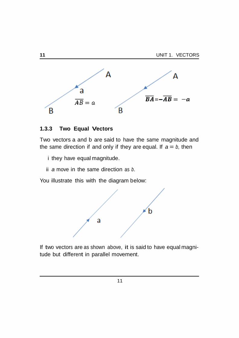
It is very important to note that BA would represent a vector

quantity of the same magnitude but of opposite direction with

AB

11

11 UNIT 1. VECTORS

1.3.3 Two Equal Vectors

Two vectors a and b are said to have the same magnitude and

the same direction if and only if they are equal. If a = b, then

i they have equal magnitude.

ii a move in the same direction as b.

You illustrate this with the diagram below:

If two vectors are as shown above, it is said to have equal magni-

tude but different in parallel movement.

12

12 UNIT 1. VECTORS

1.3.4 Types of Vectors

There are different types of vectors which are as follows:

i Position Vector: For position vector AB to occurs, point A

has to be fixed.

ii A Line Vector: A line vector is one that can shift or slide

along its line of action e.g. mechanical force acting on a

body.

iii Free Vector: It is a vector which is not restricted in any

way. It is defined by its magnitude and direction and can be

drawn as any one of a set of equal length parallel lines.

1.4 Conclusion

In this unit, you have studied the concept of vector quantities

and its diagrammatic representations. You were also introduced

to the the different types of vectors.

1.5 Summary

Having gone through this unit, you have learnt that:

i. Vectors are objects that has both magnitude and direction.

ii. A Scalar quantity has magnitude but no direction.

iii. Vector quantity can be represented by lines, drawn such that

the length of the line denotes the magnitude of the vector,

13

13 UNIT 1. VECTORS

while the direction of the line represent the direction of the

vector.

iv. Two vectors are said to be equal if and only if they have the

same magnitude and direction.

v. The types of vectors includes: position vector, line vector

and free vector.

1.6 Exercise

1. What is free and localized vector?

2. Briefly explain the term Zero Vector.

3. Write short notes on vectors in opposite direction.

4. What is Unit Vector?

1.7 References

Blitzer. Algebra and Trigonometry custom. 4th Edition

K.A Stroud. Engineering Mathematics. 5th Edition

Larson Edwards Calculus: An Applied Approach. Sixth Edition.

14

UNIT 2

Addition of Vectors

2.1 Introduction

Mathematically, the only operations that vectors posses are those

of addition and scalar multiplication.

Objectives


i. Addition of vectors

ii. Sum of a number of vectors

15

15 UNIT 2. ADDITION OF VECTORS

2.2 Main Content

The sum of two vector, AB and BC is defined as the single or

equivalent or resultant vector AC

i.e AB + BC = AC .

When finding the sum of two vectors a and b, we have to draw

them in chain, starting the second where the first ends: the sum

c is giving by the single vector joining the start of the end of the

second.

Example 2.2.1 If a = a force of 30N, acting in the east direction.

b =a force of 40N, acting in the north direction.

Then the magnitude of the vector sum r of these forces will be

50N.

Using the Pythagoras theorem of right angle triangle:

hypotenuse2 = opposite2 + adjacent2.

16


r2 + 402 + 302 = 1600 + 900 = 2500

r2 = 2500 =⇒ r = 50N

2.2.1 Sum of a Number of Vectors

The vector sum is given by single equivalent vector joining the

beginning of the first vector to the end of the last.

Hence, if vector diagram is a closed figure, the end of the last

vector join or meet with the beginning of the first, so the resultant

sum is a vector with no magnitude.

Example 2.2.2 Sum of numbers a, b, c, d, can be illustrated in

the diagram bellow:

a + b = AC

AC + c = AD

a + b + c = AD

AD + d = AE

a + b + c + d = AE

The sum of all vectors a, b, c, d is given by the single vector joining

the start of the first to the end of the last- in this case, AE. This

follows directly from our previous definition of the sum of two

vectors.

17


Example 2.2.3 Find AB + BC + C D + DE + EF

Solution

Without drawing a diagram, we can see that vectors are arranged

in chain, each beginning where the previous one left off. The sum

is therefore given by the vectors joining the beginning of the first

vectors to the end of the last. So that the sum is AF

Example 2.2.4 Find AK + K L + LP + P Q

Solution

Since it is arrange in chain, each beginning where the previous

one left off, you have that the Sum is AQ.

Example 2.2.5 Find the sum BC − DC + DE + F E i.e BC −

DC + DE − EF Solution

You must take notice of the negative vectors. Remember that

−DC = C D i.e they both have same magnitude and but direction in the opposite form. Also − F E = EF

Therefore, BC − DC + DE − F E = BC + C D + DE + EF = BF

2.3 Conclusion

In this unit, you have studied addition of vectors with examples.

2.4 Summary

Having gone through this unit, you have learnt the following:

18


i. The vector sum is given by single equivalent vector joining

the beginning of the first vector to the end of the last.

ii. If vector diagram is closed, then the end of the last vector,

join or meet with the beginning of the first, so that the re-

sultant sum is a vector with no magnitude.

2.5 Exercises

Find the sum of the following vectors.

a. P Q + QR + RS + ST

b. AC + C L − M L

c. GH + H J + J K + K L + LG

d. AB + BC + C D + DB

2.6 References




19

UNIT 3

Components of a Given Vector

3.1 Introduction

Components of a given vector deals with the resolution of a vector

with its direction (i.e. horizontal and vertical components) and

also using a single vector to replace any number of component

vector as long as they form chain in the vector diagram.

3.2 Objectives


i. Components of a given vector

ii. Proves and its applications

20

20 UNIT 3. COMPONENTS OF A GIVEN VECTOR

3.3 Main Content

3.3.1 Component of an given vector.

A single vector MN can be used to replace any number of com-

ponent vectors so long as they form a chain in the vector, as

shown above which begins with M and end with N, just like as

AB + BC + C D + DE is been replaced by AE.

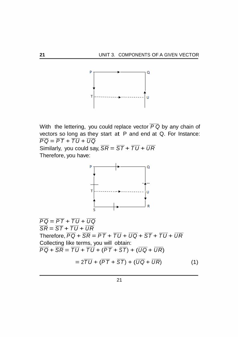
Example 3.3.1 ABCD is a square (quadrilateral) with T and U

the mid points of SP and QR respectively. Show that P Q + RS =

2T U

Solution

Consider the diagram bellow:

Reconstructing this diagram, you will have the following:

21


With the lettering, you could replace vector P Q by any chain of

vectors so long as they start at P and end at Q. For Instance:

P Q = P T + T U + U Q

Similarly, you could say, SR = ST + T U + U R

Therefore, you have:

P Q = P T + T U + U Q

SR = ST + T U + U R

Therefore, P Q + SR = P T + T U + U Q + ST + T U + U R

Collecting like terms, you will obtain:

P Q + SR = T U + T U + (P T + ST ) + (U Q + U R)

= 2T U + (P T + ST ) + (U Q + U R) (1)

22


From the diagram above, you have that P T and ST are equal in

length but of opposite sides or direction. This implies;

P T = −ST (2)

Similarly, you have that;

QU = −U R (3)

Substituting equation (2) and (3) into equation (1), you get that

P Q + ST = 2T U + (−ST + ST ) + (−U R + U R) P Q + ST = 2T U

Example 3.3.2 In triangle ABC, the points L, M, N are the

midpoints of the sides AB, BC and CA respectively. Show that:

2AB + 3BC + AC = 2LC

Solution

To prove this, you construct the diagram below;

23


With the lettering above, you have that

2AB + 3BC + C A (1)

Note that AB = 2AL, BC = BL + BC , C A = C L + LA (2)

Substituting (2) into (1), you have

2.2AL + 3(BL + LC ) + C L + LA

This implies 4AL + 3BL + 3LC + C L + LA (3)

Again, BL = −AL, C L = − LC , LA = −AL (4)

Substituting equation (4) into equation (3), you will obtain that:

2AB + 3BC + C A = 4AL − 3AL + 3LC − LC −

AL

Collecting like terms, you obtain that;

2AB + 3BC + C A = 4AL − 3AL − AL + 3LC −

LC

= LC − LC

= 2LC

3.4 Conclusion

In this unit, you have learnt the concept of vector components.

You also studied the examples in this unit.

3.5 Summary

Having gone through this unit, you have learnt that a single vector

24

can be used to replace any number of component vectors so long as

they form a chain in the vector. I.e., AB + BC + C D + DE = AE

25


3.6 Exercises

1. MNOP is quadrilateral in which C and D are the mid-point

of the diagonals MO and NP respectively. Show that M N +

M P + ON + OP = 4C D

2. Prove by vectors that the line joining the midpoint of two

sides of a triangle is parallel to third side and half its length.

3.7 References




25

UNIT 4

Components of a Vector in terms of Unit vectors and

Vectors in Space

4.1 Introduction

Component of a vector in terms of unit vector is a vector as a

way of determining the magnitude and direction in its coordinate

of x and y axis.

Vector in space is a collection of objects called vectors which may

be add together and multiplied by numbers. They are the subject

of linear algebra and are well characterized by their dimension.

4.2 Objectives


26

UNIT 4. COMPONENTS OF A VECTOR IN TERMS OF UNIT VECTORS

26 AND VECTORS IN SPACE

i Components of a vector in terms of unit vectors.

ii Vectors in Space

4.3 Main Contents

4.3.1 Components of a vector in terms of Unit Vectors

Vector AB is defined by its magnitude (r) and its angle (θ). From

the diagram, it is defined by two components in the AY (horizon-

tal) and AY (vertically) direction

i.e. AB is equivalent to a vector a in the AX direction + a vector

b in the AY direction.

AB = a + b (1)

If we now define i as a unit vector in horizontal direction.

a = ai (2)

27



Similarly, if we define j as a unit vector in the vertical direction,

then

b = bj (3)

So that the vector AB can be written as: AB = r

Substituting (2) and (3) into (1), yields;

r = ai + bj

Where i and j are unit vectors in the horizontal directions.

Example 4.3.1 If Z1 = 3i + 5j and Z2 = 7i + 3j. Find Z1 + Z2

Solution

Z1 + Z2 = 3i + 5j + 7i + 3j = (3 + 7)i + (5 + 3)j = 10i + 8j

Example 4.3.2 If Z1 = 2i − 4j, Z2 = 2i + 6j, Z3 = 3i − j. Find

a. Z1 + Z2 + Z3

b. Z1 − Z2 − Z3

Solution

a.

Z1 + Z2 + Z3 = 2i − 4j + 2i + 6j + 3i − j

= (2 + 2 + 3)i + (6 − 4 − 1)j

= 7i + j

28



b.

Z1 − Z2 − Z3 = (2i + 4j) − (2i + 6j) − (3 − j)

= (2 − 2 − 3)i + (− 4 − 6 + 1)j

= − 3i − 9j

4.3.2 Vectors in Space

According to the right hand rule, the axes, OC, OB, OA form a

right handed corkscrew action along the positive direction OA.

Similarly, rotation from OB to OA gives right-hand corkscrew

action along the positive direction of OC.

29



Vectors OP is defined by its components:

a. along OX

b. along OY

c. along OZ

Let i =unit vector in OX direction.

j = unit vector in OY direction.

k = unit vector in OZ direction.

So OP = ai + bj + ck.

Also OL2 = a2 + b2 and OP 2 = OL2 + C 2.

OP 2 = a2 + b2 + c2

So, if r = ai + bj + ck, then r = √

a2 + b2 +

c2

Example 4.3.3 Find the magnitude of a vector expressed in

terms of the unit vectors. That is, if P Q = 5i + 2j + 4k, then find

30

|P Q|.

31

52 2 2 2 4



Solution.

P Q = 5i + 2j + 4k

=⇒ |P Q| =

√ + 2 + 4 =

√ 5 + 4 + 16 =

√ 5 = 3

√5

4.4 Conclusion

In this unit, you have studied in depth, the notion of vector com-

ponents in terms of unit vectors and vector in space.

4.5 Summary


i. Vector AB is defined by its magnitude (r) and its angle (θ)

ii. If r is the Hypothenus of a right-angled triangle with sides a

and b, then r = ai + bj, where i and j are unit vectors in the

horizontal and vertical directions.

iii. The symbols i, j and k represent unit vector in the directions

OX, OY, OZ respectively. If OP = ai + bj + ck, then |OP | =

r = √

a2 + b2 + c2

4.6 Exercise

Determine the magnitude of a vector expressed in terms of a unit

vector in the following bellow:

32



a. AB = 3i + 4j − 2k

b. BC = 4i + 3j + 5k

c. P Q = 2i + 3j + 6k

4.7 References




32

UNIT 5

Direction Cosines

5.1 Introduction

Direction Cosines in analytic geometry of vector are the cosines

of angles between the vector and the three coordinate axes. Or

equivalently it is the component contributions of the basis to the

unit vector.

It refers to the cosine of the angle between any two vectors. They

are useful for forming direction cosine matrices that expresses

one set of orthonormal basis vector in terms of another set, or for

expressing a known vector in a different basis.

5.2 Objectives

In this unit, you shall study the following:

33

a

b

c

33 UNIT 5. DIRECTION COSINES

i. Direction cosines

ii. Application of direction cosines

5.3 Main Content

5.3.1 Direction Cosines

Direction cosines are the cosines of the angles between a line and

the coordinate axes. The direction of a vector in three dimensions

is determined by the angles which the vector makes with the three

axes of reference.

Let OP = r = ai + bj + ck

Then

r = cos α =⇒ a = r cos α

r = cos α =⇒ b = r cos β

r = cos γ =⇒ c = r cos γ

Also a2 + b2 + c2 = r2

=⇒ r2 cos2 α + r2 cos2 β + r2 cos2 γ = r2

34

=

22 2 2

r =

r =

r


Dividing both side by r2, you have: r2 (cos2 α+cos2 β+cos2 γ r2

r2 r2

cos2 α + cos2 β + cos2 r = 1

If l = cos x, m = cos β, n = cos γ

Then cos2 α + cos2 β + cos2 γ = 1 ⇐⇒ l2 + m2 + n2 = 1 Then [l,m,n] is called the direction cosines of the vector OP and

is the value of the cosines of the angles which the vector makes

with the three axes of reference.

Hence for vector r = ai + bj + ck

l = a , m = b , n = c and of course r = √

a2 + b2 + c2 r r r

Example 5.3.1 Find the direction cosine [l,m,n] of the vector

r = 2i + 4j − 3k Solution

Let a =2, b=4, c=-3, then

r = √

a

2 + b2 + c2 =

+ 4 + (− 3) = √

29

l = a 2 √

29

m = b 4 √

29

n = c = √−3 29

I 2

4

− 3 l

=⇒ [l, m, n] = √ 29 , √

29 , √

29

5.4 Summary


i. Direction cosines are the cosines of the angles between a line

and the coordinate axes.

35

√


ii. The direction cosines [l, m, n] are the cosines of the angles

between the vector and the axes OX, OY, OZ respectively.

iii. For the vector r = ai + bj + ck, where i, j, k are unit vectors,

you have that l = a , m = b , n = c , l2 + m2 + n2 = 1

and r r r

r = a2 + b2 + c2

5.5 Exercises

1. Find the direction cosines of the vector joining the two points

(4,2,2) and (7,6,14).

2. If A is the point (1,-1,2), B is the point (-1,2,2) and C is the

point (4,3,0), find the direction cosines of BA and BC .

3. If a = 3i − j + 2k, b = j + 3j − 2k, determine the magnitude

and direction cosines of the product vector (a x b)

5.6 References




36

UNIT 6

Scalar Product of two vectors

6.1 Introduction

A scalar quantity is one that has magnitude but no direction.

Scalar product is one of the two ways of multiplying vectors, which

has most applications in physics, engineering and astronomy.

6.2 Objectives

In this unit, you shall study the following

i. Scalar product of two vectors

ii. Expressing scalar product of two vectors in terms of the unit

vector i, j and k

37

37 UNIT 6. SCALAR PRODUCT OF TWO VECTORS

6.3 Main Content

6.3.1 Scalar product of two vectors

The scalar product of a and b is defined as the scalar (number)

ab cos θ. i.e a.b |a| x |b| cos θ. where |a| is the magnitude of the vector a. |b| is the magnitude of vector b. θ the angle between a and b.

So we multiply the length of a times the length of b, then multiply

by the cosine of the angle between a and b.

The scalar product is denoted a.b (called the dot product).

Example 6.3.1 Calculate the dot product of vectors a and b in

the diagram below:

38


Solution

a.b = |a| x |b| x cos θ

= 10 x 13 cos 59.5o

= 10 x 13 x 0.5075

= 65.98

Remark: When two vectors are at right angles to each other the

dot product is zero.

Example 6.3.2 Calculate the Dot product for the diagram be-

low:

39


Solution

a.b = |a| x |b| x cos θ

= 16 x 9 x cos 90o

= 16 x 9 x 0 = 0

Example 6.3.3 Uche has measured the end points of two poles

and wants to know the angle between them. What angle will he

get?

Solution

From the diagram above, you have three dimensions: a.b = ax.bx+

40

42 2 2


ay .by + az .bz = 9 x 4 + 2 x 8 + 7 x 10

=⇒ a.b = 122 You have to find |a| and |b| i.e the length or magnitude of the vector a and b respectively.

Using Pythagoras theorem, you will obtain:

|a| = √

+ 8 + 10 = √

180

Similarly, |b| = √

92 + 22 + 72 = √

134 You now apply the formula a.b = |a| x |b| x cos θ, to obtain θ

122 = √

180 x √

134 x cos θ

=⇒ cos θ = 122

√180√

134

=⇒ θ = cos− 1(0.7855) =⇒ θ = 38.2o

6.3.2 Expressing Scalar Product Of Two Vectors In Terms

Of The Unit Vector I, j, k.

If a = a1i + a2j + a3k

b = b1i + b2j + b3k

Then a.b = (a1i + a2j + a3k).(b1i + b2j + b3k) = a1b1i.i + a1b2i.j +

a1b3i.k + a2b1j.k + a2.b2j.j + a2b3j.k + a3b1k.i + a3b2k.j + a3k.k

Recall that i.i = (1)(1) cos 0o = 1.

Simplifying the above, you will obtain

i.i = 1, j.j = 1, k.k = 1 (a)

Similarly, i.j = (1)(1) cos 90o = 0. This implies that;

− i.j = 0, j.k = 0, k.i = 0 (b)

41

Now using the result (a) and (b), you get a.b = a1b1 + a2b2 + a3b3

42


Example 6.3.4 If a = 3i + 4j + 5k and b = 2i + j + 7k. Find a.b

Solution

a.b = 3 x 2+ 4 x 1+5 x 7 = 45

6.4 Conclusion

In this unit, you have learnt the concept of scalar product of two

vectors and its expression in terms of unit vectors.

6.5 Summary

Having through this unit, you have studied the following:

i. A scalar quantity is a quantity that has magnitude but no

direction.

ii. The scalar product (dot product) a.b, is equal to ab cos θ and

θ is the angle between a and b.

iii. If a = a1i + a2j + a3k and b = b1i + b2j + b3k, then a.b =

a1b1 + a2b2 + a3b3.

iv. The dot product of two vectors at right angle to each other

is zero.

6.6 Exercises

1. If a = 2i + 2j − k and b = 3i − 6j + 2k. Find the

scalar product of a and b

43


2. If a = 5i + 4j + 2k, b = 4i − 5j + 3k, c = 2i − j − 2k. Where i, j, k are unit vectors. Determine (a) the value of a.b (b)

the value of a.c (c) the value of b.c

3. If a = 2i + 4j − 3k and b = i + 3j + 2k, determine the scalar

product.

4. Find the scalar product (a.b) when:

(a) a = i + 2j − k, b = 2i + 3j + k

(b) a = 2i + 3j + 4k, b = 5i − 2j + k

6.7 References




43

UNIT 7

Vector Product of Two Vectors

7.1 Introduction

The vector product is one of the two ways of multiplying vectors

which has numerous applications in physics and astronomy.

Geometrically, the vector product is useful as a method for con-

structing a vector perpendicular to a plane if you have two vectors

in the plane.

Physically, it appears in the calculation of torque and in the cal-

culation of the force on a moving charge.

7.2 Objectives


i. Vector product of two vectors

44

44 UNIT 7. VECTOR PRODUCT OF TWO VECTORS

ii. Vector product in determinant form vector product calcula-

tion

7.3 Main Content

7.3.1 Vector Product of Two Vectors

Vector product of a and b is represented by a x b. It is also known

as the Cross Product of a and b. It is a vector having magnitude

|a||b| sin θ. Where |a| is the magnitude (length ) of vector a, |b| is the magnitude (length) of vector b, and θ is the angle between a

and b.

45


From the diagram above, when a and b start at the origin (0, 0

,0), the cross product will be: cx = ay bz − az by

cy = az bx − axbz

cz = axby − ay bx

Example 7.3.1 Find the cross product of a = (2, 3, 4) and b =

(5, 6, 7)

Solution

cx = ay bz − az by = 3 x 7 − 4 x 6 = −

3 cy = az bx − axbz = 4 x 5 − 2 x 7 =

6 cz = axby − ay bx = 2 x 6 − 3 x 5 = −

3 a x b = (− 3, 6, −

3)

46


7.3.2 Expressing Vector Product of two Vectors in Terms

of the Unit Vectors i,j and k.

If a = a1i + a2j + a3k and b = b1i + b2j + b3k

Then:

a x b = (a1i + a2j + a3k)(b1i + b2j + b3k) = a1b1i x i + a1b2i x

j + a1b3i x k + a2b1j x i + a2b2j x j + a2b3j x k + a3b1k x i + a3b2k

x j + a3b3k x k

But |i x i| = (1)(1)(sin 0o

=⇒ i x i = j x j = k x k = 0 (a)

Also |i x j| = (1)(1)(sin 90o) = 1

i x j = k j x k = i k x i = j (b)

Also remember that

i x j = − (j x i) j x k = − (k x j) k x i = − (i x k) =⇒ a x b = a1b1.0 + a1b2.k + a1b3(− j) + a − 2b1(− k) + a2b2.0 + a2b3.i + a3b1.j

+ a3b2(− i) + a3b3.0 =⇒ a x b = a1b2.k + a1b3(− j) + a − 2b1(− k) + a2b3.i + a3b1.j

+ a3b2(− i) = (a2b3 − a3b2)i + (a3b1 − a1b3)j + (a1b2 −

a2b1)k

OR

a x b = (a2b3 − a3b2)i − (a1b3 − a3b1)j + (a1b2 −

47

a2b1)k

Method 2

In this method, you have to put the vectors in a matrix, so that

the determinant of the matrix becomes the vector product (cross

48


product), as shown below

i j k

a x b = a1 a2 a3

= (a2b3 − a3b2)i− (a1b3 − a3b1)j + (a1b2 − a2b1)k

b1 b2 b3

This is the easiest way to write out the vector product of two vec-

tors.

Example 7.3.2 If a = 2i + 4j + 3k and b = i + 5j − 2k. Find

the vector product of a and b.

Solution i j k

a x b =

2 4 3

= i(− 8 − 15) − j(− 4 − 3) + k(10 − 4) =

1 5 − 2 − 23i + 7j + 6k

7.4 Conclusion

In this unit, you have studied the concept of vector product, also

known as the cross product. You also learnt the methods for

computing the vector product of any given two vectors.

7.5 Summary


i. Vector product, also known as cross product of a and b is

represented by a x b. Where a x b = |a||b| sin θ.

49


ii. If a = a1i + a2j + a3k and b = b1i + b2j + b3k, then a x b =

i j k

a1 a2 a3

b1 b2 b3

= (a2b3 − a3b2)i − (a1b3 − a3b1)j + (a1b2 − a2b1)k

7.6 Exercises

1. If a = 2i + 2j − k and b = 3i − 6j + 2k. Find a x b.

2. If a = 3i + 4k − 2k and b = 6i + 3k + 5k. Find the vector

product of a and b.

3. Find the vector product (a x b) when:

(a) a = 3i + 2j − k, b = 2i + 3j − k.

(b) a = 8i + 3j + 4k, b = 6i + 3j − k

7.7 References




49

UNIT 8

Loci

8.1 Introduction

In order to free geometry from the use of diagrams through the

use of algebraic expression, Descartes wished to give meaning to

algebraic operations by interpreting them geometrically.

The two basic ideas made up in the concept of Locus:

i. If the condition or description of a locus are given to find the

algebraic expression (equation) of the Locus .e.g. the Locus

of points at a distance of 3 from the point (0, 0) is given by

the equation x2 + y2 = 9.

ii. If an algebraic formula of a locus is given to find its geometric

(graphic) representation or the description in words. For

instance, the locus of a point that satisfies the equation x2 +

50

50 UNIT 8. LOCI

y2 = 9 lies on a circle with centre at (0, 0) and the radius of

3.

8.2 Objectives


i. The meaning of straight line

ii. The distance between two points and midpoint of two points

iii. The angle of slope, equation of a straight line

iv. Angle between two lines

8.3 Main Content

8.3.1 Straight Line

A line is said to be straight if and only if it has a constant gradient.

That is, if the gradients between any two points on the line are

equal.

8.3.2 Cartesian Coordinates

In Cartesian Coordinates, the coordinates is given by the position

of a point in a plane. That is, the sign distances of the points

from two perpendicular axes OX, OY. The x- coordinates is called

the Abscissa and the coordinate, the Ordinate. Figure 1 below

illustrates Cartesian coordinate abscissa and ordinates.

51

51 UNIT 8. LOCI

The diagram illustrate the abscissa and ordinate .i.e. (x, y) is (2,

3) respectively.

8.3.3 Distance between two Points and Midpoint of two

Points

8.3.3.1 Distance between two Points

Consider two points A and B with coordinate (x1, y1), (x2, y2)

respectively on Cartesian plane as shown figure 2:

52

2

2

52 UNIT 8. LOCI

Using Pythagoras theorem, you will have

AB = (x2 − x1)2 + (y2 − y1)2 (1) 2

Making AB subject of the formula, you will have

AB = (x2 − x1)2 + (y2 − y1)2

The equation shown above is the equation for distance between

two points.

Example 8.3.1 Find the distance between the points A(4, 3)

and B(6, 5).

Solution

Using the equation for distance between two points: Distance

= (x2 − x1)2 + (y2 − y1)2

If A(4, 3), B(6, 1) and A(x1, y1), B(x2, y2), then x1 = 4, y1 = 3

and x2 = 6, y2 = 5

Substituting the value of x1, x2, y1 and y2 into the equation of

distance between two points.

=⇒ Distance= (6 − 4)2 + (5 − 3)2 = 2√

2

53

53 UNIT 8. LOCI

8.3.3.2 Midpoint of two Points

In Analytical geometry, the midpoint of line segment, given the

coordinates of the endpoints is very important and useful.

54

AC =

2

2

M C

54 UNIT 8. LOCI

Let M be the midpoint of figure 4 above, so L:ABD/// L: AM C ,

so you have: AD BD = 2

AD = 2AC

x2 − x1 = 2x − 2x2 =⇒ 2x = 2x2 − x2 + x1 =⇒ x = 1 (x1 + x2) Similarly, BD = 2M C

y2 − y1 = 2(y − y1) =⇒ y2 − y1 = 2y − 2y1 =⇒ y = 1 (y1 + y2) The coordinates of the midpoint of a line segment is the average

of the coordinates of the endpoints .i.e. [ 1 (x1 + x2), 1 (y1 + y2)] 2 2

Example 8.3.2 If A is (3, 6) and B is (4, 8). Find the coordinate

of the midpoint of AB.

Solution

Using the midpoint of a line segment formula, [ 1 (x1 + x2), 1 (y1 +

2 2

y2)]. You have that, x1 = 3, x2 = 4, y1 = 6, y2 = 8

This implies that the coordinate of the midpoint of AB is

[ 1 1 1

2 (3 + 4),

2 (6 + 8)] = [3

2 , 7]

8.3.4 Gradient (gradient, angle of slope, and equation

of a straight line).

8.3.4.1 Gradient

The gradient of a line is defined as the ratio of the vertical distance

the line rises or falls to the horizontal distance. It is represented

by lettered m.

55

dx

55 UNIT 8. LOCI

Therefore, the gradient (m) = dy = y2 − y1

x2 − x1

8.3.4.2 Angle of Slope

The angle of slope as in figure 5 is represented by θ. It is deter-

mined by:

tan θ = sin θ

cos θ

(1)

Recall from the figure 5, that the diagram can be well represented

below and can be used to determine angle of the slope.

56

z

⇒ =

56 UNIT 8. LOCI

From the diagram above, you have that:

y sin θ =

z =

y2 − y1

z

(since y = dy) (1)

x Also cos θ = =

z

x2 − x1

z

(since x = dx) (2)

Substituting equation 2 and 3 into (1), you obtain that

tan θ = y2 − y1 x z

x2 − x1

= tan θ = y2 − y1 dy

x2 − x1 dx

=⇒ θ = tan− 1 I

y2 − y1

l = tan− 1

I dy l

= tan− 1(m) x2 − x1 dx

Hence the Angle of a slope is defined as the inverse of tangent of

the gradient (m) of a straight line.

Remark 8.3.3 If 0o < θ < 90o, tan θ is positive and the line has

a positive gradient.

If θ = 90o, the line has no gradient but perpendicular to the x-

axis.

57

dx =

⇒

5

dx

57 UNIT 8. LOCI

If 90o < θ < 180o, tan θ is negative and the line has a negative

gradient.

Example 8.3.4 Calculate:

1. The gradient of the line joining A(4,3) and B(9,7).

2. The angle of the slope

Solution

1. Using the formula

m = dy

y2 − y1

x2 − x1

From the above, you have that x1 = 4, x2 = 9, y1 = 3, y2 = 7

= m = 7− 3 4 9− 4 5

2. θ = tan− 1(m) = tan− 1

4 )

=⇒ θ = 38.66o

8.3.4.3 Equation of a Straight Line

A. Gradient-intercept form.

Using the diagram in figure 5, the equation of a straight line

in a gradient intercept form is: y = mx + c. Where m =

gradient= dy , and

c = intercept on real y-axis.

B. Gradient and one point form.

58

58 UNIT 8. LOCI

Using the diagram above, the equation of a straight line

of gradient and one point form when a straight line passes

through a given point p (x1, y1) is :

y − y1 = m(x − x1)

.

C. Gradient and two Points Form

If (x1, y1) and (x2, y2) are two points given on a line AB as

shown in figure 8, which is used to get the equation of a

straight line on a gradient and two point.

59

=⇒ y− y1

= .

59 UNIT 8. LOCI

The gradient (m) of the line AB above is:

m = y2 − y1

x2 − x1

(1)

From one point form: y − y1 = m(x − x1) (2)

Substituting equation (1) into equation (2), you have

(y2 − y1)(x − x1)

y2 − y1 =

y − y1 =

x− x1

x2 − x1

x2 − x1 (3)

Therefore, the equation of a line through the two points is: y− y1

y2 − y1

x− x1

x2 − x1

Example 8.3.5 A straight line has a gradient of 5/3 and it passes

through the point (1,3). Find its equation and its intercept on

the y axis.

60

3

3

3

60 UNIT 8. LOCI

Solution

Since the line passes through a gradient and one point, you will

make use of gradient and one point form equation. That is

y − y1 = m(x − x1) Given that (x1, y1) = (1, 4) and m = 5 , you have that

y − 4 = 5 (x − 4) =⇒ 3(y − 4) = 5 3(x − 4) 3 3

=⇒ 3y = 5x − 8

=⇒ 3y

5x 8

3 =

3 −

3

Hence the equation of the straight line at the point (x1, y1) =

(1, 4) and the gradient (m) = 5 is:

=⇒ y = 5 x − 8 . 3 3

To obtain the intercept, you have to use the equation: y = 5 x − 8 3 3

Comparing the above with the equation of straight line: y =

mx + c, you have that

c = − 8 .

8.3.5 Angle Between two Lines

The angle between two lines in a plane is defined to be:

i. 0, if the lines are parallel

ii. the smaller angle having as sides the half-lines starting from

the intersection point of the lines and lying on those two

lines, if the lines are not parallel.

61

1+tan β2 tan β1

1+m m

1+tan β2 tan β1

1+m m

61 UNIT 8. LOCI

If line A1 has a gradient m1 and line A2 has gradient m2 making

an angles of β1 and β2 respectively on the x- axis as shown in

figure 9. β is the acute angle between the lines.

Recalling that tan θ = m (gradient), this implies that m1 = tan θ

and m2 = tan θ. The exterior angle of the triangle, β2 = β1 + β

So β = β2 − β1

Therefore tan β = tan(β2 − β1) But tan β = tan β2 − tan β1

=⇒ tan(β2 − β1) = tan β2 − tan β1

Replacing back the values of β2 and β1, you have tan β = m2 −m1

2 1

Note: When the result is negative, an obtuse angle 180 − β is obtained. Hence the acute angle β between lines of gradient m1, m2

is given by: tan β = m2 −m1

2 1 Where m1m2 /= 1.

62

1+m m

m2

4

4

4 4

62 UNIT 8. LOCI

8.3.5.1 Parallel Lines

When tan β is zero, the lines are parallel and then m1 = m2.

8.3.5.2 Perpendicular Lines

When the lines are perpendicular, the angle β is 90o. Hence

tan 90= m2 −m1 2 2

which has no finite value. So 1 + m2m1 = 0.

Therefore, if two lines of gradients m1, m2 are perpendicular, then

m1m2 = − 1 or m1 = − 1

Example 8.3.6 Find the angle between the two lines − 3x+4y = 8 and − 2x − 8y − 14 = 0 Solution

Finding the slope (gradient) of each equation by comparing them

to y = mx + c, you have

3x + 4y − 3x = − 3x + 8 =⇒ 4y = − 3x + 8 =⇒ y = − 3 x + 2 =⇒ m1 = − 3

Similarly, you follow the same argument to obtain m2

− 2x − 8y − 14 = 0 =⇒ 8y = − 2x − 14 =⇒ y = − 2x − 1l4

8 8 − 1 m2 −m1

=⇒ m2 = two lines.

4 Now, using tan β = 1+m2 m1

to find angle between

Substituting the values of m1 and m2 to the equation, you have; −3 1

tan β = 4 − (−

4 )

1+(− 3 x −1 )

63

16

16

19

19

2

2

2

63 UNIT 8. LOCI

−3 1

tan β =

tan β =

4 + 4

1+( 3 ) −1

2

1+( 3 )

tan β = − 8

β = tan− 1 tan β = − 8 )

β = − 14.63o

Example 8.3.7 Find the equation of the line through the point

(− 1, 2) which is a) parallel to y = 2x + 1 b) perpendicular to y = 2x − 1 Solution

a) The gradient (m) = 3 and (x, y) = (− 1, 2) Now to obtain the equation, you make use of the formula: y − y1 = m(x − x1) y − 2 = 3(x − (− 1)) y − 2 = 3(x + 1) =⇒ y = 3x + 5

b) The gradient of the perpendicular line is − 1 .

Using y − 2 = − 1 (x − (− 1)) =⇒ y − 2 = − 1 (+1) =⇒ y − 2 = − 1 x − 1

2 2

=⇒ y = − 1 x + 3 2 2

64

dx

1+m m

64 UNIT 8. LOCI

8.4 Conclusion

In this unit, you have learnt the meaning of straight line and the

equation of straight line. You have also learnt the concept of angle

of slope and angle between a straight line. Finally, you were also

introduced to the distance between two points and midpoint of

two points.

8.5 Summary


i. Gradient (m) = dy = y2 − y1

x2 − x1

ii. Angle of slope θ = tan− 1 (

y2 − y1

\

x2 − x1

iii. Distance between (x1, y1) and (x2, y2) is (x2 − x1)2 + (y2 − y1)2

iv Midpoint of (x1, y1) and (x2, y2) is 1 (x1 + x2), 1 (y1 + y2))

2 2

v. Gradient and y-intercept form is y = mx + c

vi. Gradient and one point form is y − y1 = m(x − x1)

vii. Two point form is y− y1

y2 − y1 = x− x1

x2 − x1

viii. Acute angle β between lines of gradients m1, m2 is given by

tan β = m2 −m1

2 1

ix For parallel lines, m1 = m2. For perpendicular line, m1m2 =

− 1

65

2

65 UNIT 8. LOCI

8.6 Exercises

1. Find the distance between the points of the following:

(a) (1, -4) and (7,6)

(b) (-1,-3) and (5,4)

2. What are the coordinate of the midpoint of the line joining:

(a) (3, 5) and (6, 7)

(b) (-3,-9) and (6, 8)

3. Find the gradients of the line joining the points:

(a) (2,5) and (5,9)

(b) (1,3) and (5,3)

4. Find the equations of the line which passes through the fol-

lowing pairs of points:

(a) (-1,-2) and (3, 0)

(b) (3, -2) and (-5,-2)

5. State the gradient and the intercept of the following lines

(a) 3x − 2y − 8 = 0

(b) x + y = 1 4 3

6. A straight line has a gradient of − 5

and passes through the

point (2, 5). Find its equation and its intercept on y-axis.

66

1

66 UNIT 8. LOCI

7. Find the equation of a line AB which passes through (3, -3)

and (-4,-7). Hence find the equation of the straight line CD

parallel to AB, which passes through the point (4, 9).

8. Find the equation of the line which passes through (-6,7) and

is parallel to the line y = 3x + 7.

9. Find the equation of the line which is parallel to the line

2y + 3 = 3 and passes through the midpoint of (-2,3) and (4,

5).

10. Find the acute angle between the lines:

(a) 2y = 3x − 8 and 5y = x + 7

(b) 2x + y = 4 and y − 3x + 7 = 0

11. A line AB passes through the point P (3, -2) with gradient

− 2 . Find its equation and also the equation and also the equation of the line CD through P perpendicular to AB.

8.7 References

Blitzer. Algebra and Trigonometry Custom. 4th Edition

Godman and J.F Talbert. Additional Mathematics



67

UNIT 9

Coordinate Geometry (Circle)

9.1 Introduction

A circle is the locus of all points equidistant from a central point.

9.2 Objectives


i. Equation of a circle

ii. Parametric eqaution of a circle

iii. Points outside and inside a circle

iv. Touching circles

v. Tangents to a circle

68

68 UNIT 9. COORDINATE GEOMETRY (CIRCLE)

9.3 Main Content

9.3.1 Equation of a circle

9.3.1.1 Center at the Origin and a Radius r

Let us consider a simplest case of a circle with centre at the origin

and radius r as shown in figure 1. If the circle has a centre (0, 0)

and radius r.

Using Pythagoras theorem, the equation of the circle from the

figure above, becomes;

x2 + y2 = r2

9.3.1.2 Center and one point given

Equation of a circle by moving the centre to a new point (h, k)

which has a radius r as shown in figure 2.

69


The length (radius) of the hypotenuse of the right triangle is

determine by the Pythagoras formula:

X 2 + Y 2 = r2 (1)

Where Y = y − k and X = x − h. Substituting these values into

equation (1), you have

(x − h)2 + (y − k)2 = r2

Note: (h ,k) is the centre of the circle and r is the radius.

Example 9.3.1 Find the center and radius of the circle x2 +

y2 + 8x + 6y = 0. Sketch the circle.

70


Solution

The aim is to get the equation into the form: (x − h)2 + (y − k)2 = r2.

x2 + y2 + 8x + 6y = 0

=⇒ x2 + 8x + y2 + 6y = 0 (1)

Applying completing the square method to equation, you have

that:

x2 + 8x + 16 + y2 + 6y + 9 = 16 + 9

=⇒ x2 + 8x + 16 + y2 + 6y + 9 = 25

=⇒ (x + 4)2 + (y + 3)2 = 52 (2)

Hence, this is now in the form: (x − h)2 + (y − k)2 = r2 that

is required and you can determine the centre and the radius by

comparing it with equation (2). So the centre of the circle is:

h = − 4 and k = − 3 Thus the radius is r = 5

Note: that the circle passes through (0, 0). This is logical, since

(− 4)2 + (− 3)2 = (5)2.

71


9.3.1.3 General equation of a circle

The equation of a circle is x2 + y2 + 2gx + 2f y + c = 0, where the centre is the point (-g,-f ) and the radius r = g2 + f 2 − c

Note:

For a second degree equation to represent a circle:

a the coefficients of x2 and y2 must be identical

b there is no product term in xy.

Example 9.3.2 The equation of a circle is x2 +y2 +2x− 6y− 15 = 0. What are the center and the radius?

Solution

Comparing x2 +y2 +2x− 6x− 15 = 0 with x2 +y2 +2gx+2f y+c = 0

72

√


Taking the coefficient:

Coefficient of x: 2g = 2 =⇒ g = 1 Coefficient of y: 2f = − 6 =⇒ f = − 3 Coefficient of c: c = − 15 To get the radius, you apply the formula, r = g2 + f 2 − c

So that r = 12 + (− 3)2 − (− 15)2 = √

25 = 5 Hence, the center (− g, − f ) = (− 1, 3) and the radius r = 5.

Example 9.3.3 Find the equation of the circle with center (− 2, 3)

and radius 6.

Solution

Using the equation, (x − h)2 + (y − k)2 = r2.

Where h = − 2, k = 3, r = 6

You now have that,

[x − (− 2)]2 + [y − 3]2 = 62

=⇒ x2 + 4x + 4 + y2 − 6y + 9 = 36 =⇒ x2 + y2 + 4x − 6y − 23 = 0

Example 9.3.4 Find the equation of the circle with center (-3,4)

which passes through the point (2,5)

Solution

You first have to find the radius r, using the distance between two

points formula since radius r is the distance from (-3,4) to (2, 5).

r = (x2 − x1)2 + (y2 − y1)2 = =⇒ r2 = 26

[2 − (− 3)]2 + (5 − 4)2 = 52 + 12

Hence, using the equation, (x − h)2 + (y − k)2 = r2, where r2 = 26, h = − 3, k = 4 [x − (− 3)]2 + (y − 4)2 = 26

73


=⇒ x2 + 6x + 9 + y2 − 8y + 16 = 26

=⇒ x2 + y2 + 6x − 8y − 1 = 0

Example 9.3.5 Find the points of intersection of the circle x2 +

y2 − x − 3y = 0 with the line y = x − 1. Solution

Solving the equations simultaneously, you have;

x2 + y2 − x − 3y = 0 (1)

y = x − 1 (2)

Substituting equation (2) into equation (1), you will have;

x2 + (x − 1)2 − x − 3(x − 1) = 0 =⇒ x2 + x2 − 2x + 1 − x − 3x + 3 = 0 =⇒ 2x2 − 6x + 4 = 0 =⇒ x2 − 3x + 2 = 0 =⇒ (x − 1)(x − 2) x = 1 or x = 2

To get the corresponding y values, you make use of equation(2)

and substituting the values of x.

y = 1 − 1 or y = 2 − 1 =⇒ y = 0 or y = 1 So that the points of intersection are at (1, 0) and (2, 1).

74


9.3.2 Parametric Equation of a Circle

In Figure 3, the circle with centre C(a, b) and radius r. If P

is any point on the circle and the radius C P makes an angle

θ(0 ≤ θ ≤ 360o) with C N which is parallel to the axis. C N = r cos θ and P N = r sin θ. So the coordinate (x, y) of P will

be given by the two equations:

x = a + r cos θ, y = b + r sin θ (1)

These is called the parametric equations of the circle as they give

the coordinates of every point on the circle in terms of one variable

or parameter θ (where r is always greater than zero).

From these equations, you can deduce the ordinary x-y equation

by eliminating between them.

75

2 2


From equation (1), you have cos θ = x− a , sin θ = y− b .

r r

Recall that sin2 θ + cos2 θ = 1

Hence, (x− a)

+ (y− b)

r2 r2 = 1 =⇒ (x − a)2+)(y − b)2 = r2. This is still the usual form of the equation of a circle.

Example 9.3.6 a. State the parametric equations of a circle

with centre (2, -1) and radius 3.

b. State the centre and radius of a circle given by x4 = 2c cos θ, y+

3 = 2 sin θ

Solution

a. Using the formula of parametric equations of the circle, x =

a + r cos θ, y = b + r sin θ.

Then x = 2 + 3 cos θ

y = − 1 + 3 sin θ b. Rewriting the parametric equation:

x = 4 + 2 cos θ, y = − 3 + 2 sin θ. The center is (4, − 3) and the radius is 2.

9.3.3 Points Outside and Inside a Circle

Let the function f (x, y) = (xa)2 + (y − b)2 − r2. f (x, y) =

0= defines a circle, radius r and centre (a, b). When the point (h,

k) lies inside this circle as shown in the figure 4.

76


Then, (h − a)2 + (k − b)2 < r2 i.e. (h − a)2 + (k − b)2 − r2 < 0 or f (h, k) < 0.

So, if (h, k) lies inside the circle given by f (x, y) = 0, then

f (h, k) < 0. Similarly if (h, k) lies outside the circle, f (h, k) > 0.

Example 9.3.7 Are the points A(1,-1) B(5, 2) inside or outside the circle x2 + y2 − 3x + 4y = 12?

Solution

Take f (x, y) = x2 + y2 − 3x + 4y − 12 f (1, − 1) = 1 + 1 − 3 − 4 − 12 = − 17 < 0. So A is inside the circle. f (5, 2) = 25 + 4 − 15 + 8 − 12 = 10 > 0. So B is outside the circle.

9.3.4 Touching Circles

Two circles with centres A, B and radii r1, r2 can touch each other

internally or externally, as shown below.

77


Example 9.3.8 Find how the circles x2 + y2 + 2x + 6y = 39 and

x2 + y2 − 4x − 2y + 1 = 0 touch each other. Find the coordinates of their point of contact.

Solution

Comparing the two equations with x2 + y2 + 2gx + 2f y + c = 0

to find their respective centre and their respective radius.

First, you find the centre and radius at point A:

x2 + y2 + 2gx + 2f y + c = 0 (1)

x2 + y2 + 2x + 6y − 39 = 0 (2)

Comparing the coefficient of each other:

Coefficient of x: 2g = 2.

=⇒ g = 1 Coefficient of y: 2f = 6.

=⇒ f = 3 Coefficient of constant term: c = − 39. Hence, (− g, − f ) = (− 1, − 3). and

r = g2 + f 2 − c = 12 + 32 − (− 39) = √

49 = 7 Center A(− 1, − 3) and its radius r = 7.

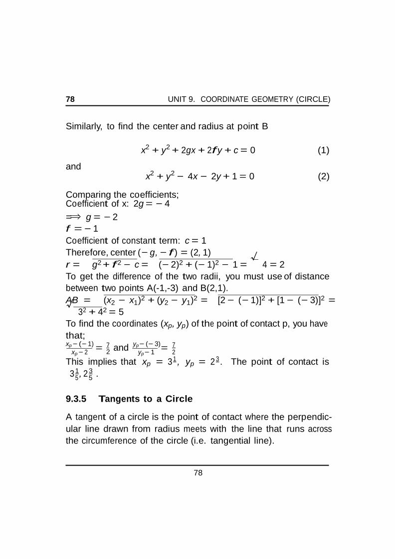
78

= 7 =


Similarly, to find the center and radius at point B

and

x2 + y2 + 2gx + 2f y + c = 0 (1)

x2 + y2 − 4x − 2y + 1 = 0 (2)

Comparing the coefficients; Coefficient of x: 2g = − 4

=⇒ g = − 2 f = − 1 Coefficient of constant term: c = 1

Therefore, center (− g, − f ) = (2, 1)

r = g2 + f 2 − c = (− 2)2 + (− 1)2 − 1 = √

4 = 2 To get the difference of the two radii, you must use of distance

between two points A(-1,-3) and B(2,1).

AB = (x2 − x1)2 + (y2 − y1)2 = [2 − (− 1)]2 + [1 − (− 3)]2 = √32 + 42 = 5

To find the coordinates (xp, yp) of the point of contact p, you have

that; xp − (− 1)

xp − 2 2 and

yp − (− 3) 7 yp − 1 2

This implies that xp = 3 1 , yp = 2 3 . The point of contact is 3 1 3

5 , 2

5

.

9.3.5 Tangents to a Circle

A tangent of a circle is the point of contact where the perpendic-

ular line drawn from radius meets with the line that runs across

the circumference of the circle (i.e. tangential line).

79

2


Example 9.3.9 Find the equation of the tangent to the circle

x2 + y2 − 2x + 4y = 15 at the point (-1, 2).

Solution

x2 + y2 − 2x + 4y = 15 Rearranging this equation of the circle and comparing with the

general equation of the circle, you will have

x2 + y2 − 2x + 4y − 15 = 0 (1)

x2 + y2 + 2gx + 2f y + c = 0 (2)

Coefficient of x: 2g = − 2 =⇒ g = − 1

Coefficient of y: 2f = 4 =⇒ f = 2 Therefore the centre (− g, − f ) = (1, − 2). The gradient of the radius to the point (− 1, 2) is -2. Hence, the gradient of the tangent is 1 . Its equation is therefore:

y − 2 = 1/2(x + 1) i.e 2y = x + 5.

9.4 Conclusion

In this unit, you have learnt the concept of circle. You were also

introduced to the equation and parametric equations of a circle.

9.5 Summary


80


i. The equation of a circle with center 0, radius r is: x2 + y2 =

r2.

ii. Circle, centre (a, b), radius r has equation : (x − h)2 + (y −

k)2 = r2.

iii. General equation of circle: x2 + y2 + 2gx + 2f y + c = 0.

9.6 Exercises

1. Given a circle with centre (-3,-4), which passes through the

point ( 2,-1). Find the equation.

2. If the circle centre (1, -3) passes through the origin, find its

equation.

3. Find the centre and radius of each of the following circles:

(a) x2 + y2 − 2x − 6y = 15.

(b) x2 + y2 − 6x + 14y = 49 = 0.

4. (a) State the parametric equations of a circle with centre

(-1,-3) and radius 5.

(b) State the centre and radius of the circle given by x =

2 + 4 cos θ, y = − 5 + 4 sin θ

5. . Show that the circle x2 + y2 − 2x − 4y + 4 = 0 lies

completely inside the circle x2 + y2 = 15.

6. Find the equation of the tangents to the circles:

(a) x2 + y2 + 4x − 10y − 12 = 0 at (3, 1).

81


(b) x2 + y2 − 6x − 4y − 16 = 0 at (-

2,0).

9.7 References


Godman and J.F Talbert. Additional Mathematics



82

UNIT 10

Parabola

10.1 Introduction

A parabola has many applications in real life situations where:

a. radiation needs to concentrated at one point(e.g. radio tele-

scope, pay TV dishes, solar radiation collectors) or

b. radiation needs to be transmitted from a single point into

wide parallel beam(e.g headlight reflectors).

10.2 Objectives


i. definition of a parabola

83

83 UNIT 10. PARABOLA

ii. the formula for a parabola vertical axis

iii. parabola with horizontal axis

iv. shifting the vertex of a parabola from the origin.

10.3 Main Content

10.3.1 Definition of Parabola

A parabola is defined as the locus of a point which moves so that

it is always the same distance from the fixed point (called the

focus) and a given line (called the directrix).

In the graph above:

84


i. The focus of the parabola is at (0, p)

ii. The line y = − p is the directrix.

iii. The focal distance is |p| (Distance from the origin to the

focus and from the origin to the directrix. You take absolute

value because distance is positive.)

iv. The point (x, y) represent any point on the curve.

v. The distance d from any point (x, y) to the focus (0, p) is

the distance from (x, y) to the directrix.

vi. The axis of symmetry (goes through the focus, at right angles

to the directrix).

vii. The vertex ( where the parabola makes its sharpest turn) is

halfway between the focus and directrix.

viii. Reflector is any ray parallel to the axis of symmetry which

gets reflected off the surface straight to the focus. This ex-

plains why that dot is called the focus, because that is where

all the rays get focused.

10.3.2 The formula for a parabola vertical axis.

From the diagram, in figure 1, If the distance d = y + p. Using

the distance formula on the general points (0, p) and (x, y), and

equating it to our value d = y + p, you have:

(x − 0)2 − (y − p)2 = y + p Squaring both sides gives;

(x − 0)2 − (y − p)2 = (y +

85

p)2

86

4p


Simplifying gives you the formula for a parabola:

x2 − (y2 − 2py + p2) = y+2py + p2

Collecting like terms of the equation above. x2 − y2 + 2py − p2 = y2 + 2py + p2.

x2 = y2 − y2 + 2py + 2py + p2 − p2.

x2 = 4py.

Making y subject of the formula: y = x2

Where p is the focal distance of the parabola.

Example 10.3.1 What is the equation of the directrix of the parabola whose equation is: x2 − 30y = 0.

Solution

x2 − 30y = 0. Rearranging this and making x2 subject of the formula, you will

obtain:

x2 = 30y (1)

Equating equation (1) with the general formula of parabola, you

will have;

30y = 4py =⇒ p = 7.5 The directrix is on the opposite side of the origin to the focus (0,

7.5).

So, the directrix of x2 − 30y = 0 is y = − 7.5.

Example 10.3.2 Where is the focus of the parabola whose equa-

tion is y2 + 32x = 0

Solution

y2 + 32x = 0.

Rearranging the terms and comparing with the general formula

y2 = 4px., you will obtain that

87


4px = − 32x =⇒ P = − 8 So the focus of y2 + 32x = 0 is F (− 8, 0).

10.3.3 Parabola with horizontal axis.

In this case as shown in figure 2, the parabola place on the Carte-

sian coordinate (x- y graph) with:

a. Its vertex at the origin 0 and

b. Its axis of symmetry lying on the x axis, then the curves is

defined by: y2 = 4px.

88

4

4

4


Example 10.3.3 Where is the focus in the equation y2 = 5x?

Solution

Comparing y2 = 5x with equation of a parabola on a horizontal

axis, you have that:

y2 = 5x (1)

y2 = 4px (2)

Equating equation (1) to equation(2), you will have:

5x = 4px =⇒ p = 5

Substituting the value of p into equation (2), you will obtain that

: y2 = 4 5 x =⇒ y2 = 5x

So that F (p, 0) = 5 , 0).

The equations of a parabola in different orientations are as fol-

lows:

89


10.3.4 Shifting the vertex of a parabola from the origin.

This is similar concept to the case when we shifted the centre of

a circle from the origin. To shift the vertex of a parabola from

(0, 0) to (h, k), each x in the equation becomes (y − k). So if the axis of a parabola is vertical and the vertex is at (h, k),

you have:

(x − h)2 = 4p(y − k).

90


If the axis of a parabola is horizontal and the vertex is at (h, k),

the equation becomes:

(y − k)2 = 4p(x − h) .

Example 10.3.4 Find the equation of the parabola having vertex (0, 0), axis along the x- axis and passing through (2, − 1).

Solution

91

8

8

2


The curve must have this orientation, since you know it has horizontal axis and passes through (2, − 1):

Using the general formula y2 = 4px. you need to find the value of

p since the curve goes through (2, − 1). Since x = 2 and y = − 1, then substituting the value of x and y into the general formula. (− 1)2 = 4(p)(2). =⇒ 1 = 8p =⇒ p = 1

Now substituting the value of p into the general equation to get

equation of the parabola.

y2 = 4 1 x

This implies that, the equation of the parabola is y2 = x

10.4 Conclusion

In this unit, you studied the concept of parabola. You were also

introduced to the equation of a parabola with vertical and hori-

zontal axis.

92


10.5 Summary


i. A parabola is defined as the locus of a point which moves

so that it is always the same distance from the fixed point

(called the focus) and a given line (called the directrix).

ii. The equation of a parabola with horizontal axis is: y2 = 4px

iii. The equation of a parabola with vertical axis is: x2 = 4py

iv. If the axis of a parabola is vertical and the vertex is at (h, k),

the the equation of the parabola is: (x − h)2 = 4p(y − k)

v. If the axis of a parabola is horizontal and the vertex is at

(h, k), the the equation of the parabola is: (y − h)2 = 4p(x − k)

10.6 References




92

UNIT 11

Ellipse and Hyperbola

11.1 Introduction

Ellipse and hyperbola take a huge rule curves and curves fittings

that devise reliable methods for establishing the relationship be-

tween two variables for minimizing errors.

11.2 Objectives

In this unit, you shall study the concept of ellipse and hyperbola,

together with their properties.

93

93 UNIT 11. ELLIPSE AND HYPERBOLA

11.3

Main Content

11.3.1

Ellipse

Definition 11.3.1 An Ellipse can be defined as the locus of all

points that satisfies the equation: x2

+ y2

= 1.

Where: a2 b2

x, y are the coordinates of any point on the ellipse,

a = radius on the x axis or the semi major axis , and

b = radius on the y axis or the semi minor axis.

This equation is very similar to the one used to define a circle.

The only difference between a circle and an ellipse, is that in an

ellipse, there are two radius measures, one horizontally along the

x- axis, the other vertically along the y axis as shown in figure 1.

94

a2 + y

a2 +

b2

2


Clearly, for a circle both of these have the same value. By con-

vention, the y radius is usually called b and the x - axis is called

a.

11.3.1.1 Ellipses Centred at the Origin.

If the ellipse is centred on the origin, (its centre at (0, 0)) the

equation is: x2 2

= 1, where: a = radius on the x- axis, this

implies that y = 0, x = ±a b = radius on the y- axis, this implies x = 0, y ± b. Note that the equations above are true only for ellipses that are aligned with the coordinate plane, that is, where

the major and minor axes are parallel to the coordinate system.

11.3.1.2 Ellipses not Centred at the Origin

Just as with the circle equations, we subtract offsets from the x

and y terms to translate (or move) the ellipse back to the origin.

So the full form of the equation is: (x− h)

(y− k)2

b2 = 1.

Where a is the radius along the x axis, b is the radius along the

y axis, h, k are the x, y coordinates of the ellipses center.

11.3.1.3 Derivation of Ellipse formula.

You recall the basic equation of a circle: x2 + y2 = r2

From the above equation, you have x2

+ y2

= 1 r2 r2

Replace the radius with the a separate radius for the x- axis and

b separate radius for the y- axis. x2 y2

a2 + r2 = 1.

95

2


With a > b > 0. The length of the major axis is 2a and the length

of the minor axis is 2b. The two foci (foci is the plural of focus)

are at (∼ ± ∼ c, 0) or at (∼ +mn ∼ c)

Example 11.3.2 Given that ellipse has an equation of 9x2 +

4y2 = 36.

a. Find the x and y intercepts of the graph of the equation.

b. Find the coordinates of the foci.

c. Find the length of the major and minor axis.

d. Sketch the graph of the equation.

Solution

a. Recall that the equation of ellipse is

x2

a2 +

y2

b2 = 1 (1)

Hence, rewrite the equation in the form of the ellipse equation:

9x2 + 4y2 = 36.

x2 y2

=⇒ 22

+ 32

= 1 (2)

Comparing equation (1) and equation (2) together.

Then a =3, and b =2 (where a > b).

Set y=0 in equation (2) obtained and find the x- intercepts.

Then equation (2) becomes: x2

+ 02

= 1

=⇒ x = 1 22 32

22

=⇒ x2 = 22

=⇒ x =∼ +mn ∼ 2

96

1

2


Set x = 0 in equation (2) obtained and find the y- intercepts.

Then equation (2) now becomes: 02

+ y2

= 1

=⇒ y = 1 22 32

32

=⇒ y2 = 32

=⇒ y =∼ +mn ∼ 3. Hence, x and y intercept is: (x, y) = (2, 3).

b. To find the coordinate of the foci, you need to find c first.

c2 = a2 − b2. Substituting a and b that was found in part (a) into the equation, you obtain:

c2 = a2 − b2 = 32 − 22 = 9 − 4 = 5.

=⇒ c2 = 5. =⇒ c =∼ +mn ∼ (5) 2

The foci are F1

I0, (5) 2

l and F2

I0, − (5) 2

l 1 1

c. The major axis length is given by 2a = 2 x 3 = 6

The minor axis length is given by 2b = 2 x 4 = 8

d. Locate the x and y intercepts, find the extra points if needed

and sketch.

97


11.3.2 Hyperbola

Hyperbola is a symmetrical open curve formed by the intersection

of a circular cone with a plane at a smaller angle with its axis than

the side of the cone.

Mathematically, it is defined as a curve where the distance of any

point from:

i. a fixed point (the focus).

ii. a fixed straight line (the directrix) are always in the same

98

a

a

2


ratio.

This ratio is called the eccentricity, and for the hyperbola it is

always greater than 1. The hyperbola is an open curve (has no

ends). Hyperbola is actually two separate curves in mirror image.

11.3.2.1 Equation of Hyperbola

By placing a hyperbola on an x- y graph (centred over the x- axis

and y axis), the equation of the curve is: x2 y = 1

Also: a2 −

b2

One vertex is at (a, 0), and the other is at (− a, 0).

The asymptotes are the straight lines: y = b x

y = − b ) x.

11.3.2.2 Eccentricity

Eccentricity (e) shows how uncurvy (varying from being a circle)

the hyperbola is.

99

P N


In the diagram above, you have that

a. P is the point on the curve

b. F is the focus and

c. N is the point on the directrix so that PN is perpendicular

to the directrix.

The ratio P F

is the eccentricity of the hyperbola ( for a hyperbola

the eccentricity is always greater than 1). It can also be given by √

the formula: e = a2 +b2

a

Example 11.3.3 Given the following equation 9x2 − 16y2 = 144

a. Find the x and y intercepts of the graph of the equation.

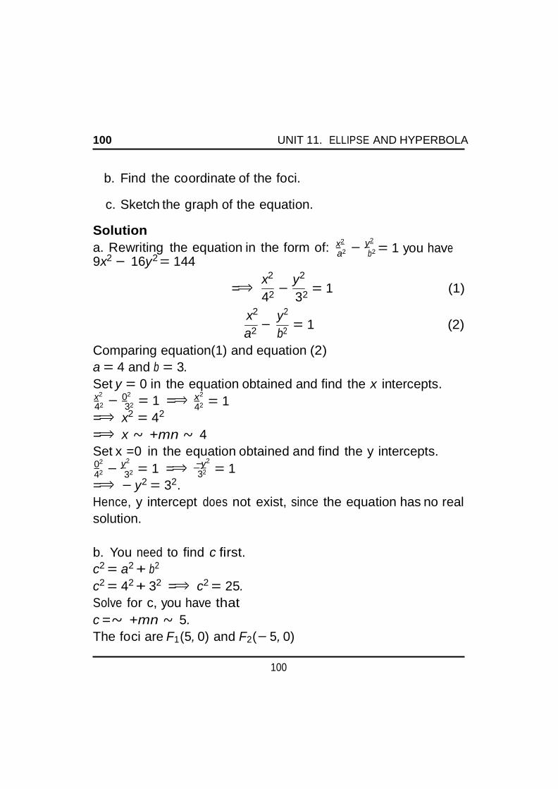
100

32

2


b. Find the coordinate of the foci.

c. Sketch the graph of the equation.

Solution

a. Rewriting the equation in the form of: x2

y = 1 you have

9x2 − 16y2 = 144

x2 y2

a2 − b2

=⇒ 42 −

32 = 1 (1)

x2 y2

a2 −

b2 = 1 (2)

Comparing equation(1) and equation (2)

a = 4 and b = 3.

Set y = 0 in the equation obtained and find the x intercepts. x2 02 x2

42 − 32 = 1 =⇒

=⇒ x2 = 42

42 = 1

=⇒ x ∼ +mn ∼ 4 Set x =0 in the equation obtained and find the y intercepts. 02 y2

y2

42 − 32 = 1 =⇒ − = 1

=⇒ − y2 = 32. Hence, y intercept does not exist, since the equation has no real

solution.

b. You need to find c first.

c2 = a2 + b2

c2 = 42 + 32 =⇒ c2 = 25. Solve for c, you have that

c =∼ +mn ∼ 5. The foci are F1(5, 0) and F2(− 5, 0)

101

4

2 and y = −

2 2

2 2

2


c. Find extra points (if necessary)

Set x = 6 and find y.

9(6)2 − 16y2 = 144 =⇒ − 16y2 = 144 − 324.

=⇒ y2 = 45

1

=⇒ y = 3(5) 2

1 3(5) 2

2

So the points

( 1

6, 3(5) 2

and

( 1

6, − 3(5) 2

are on the graph of

the hyperbola.

Also because of the symmetry of the graph of the hyperbola, the

points

( 1

− 6, 3(5) 2

and

( 1

− 6, − 3(5) 2

are also on the graph of the

hyperbola.

11.4 Conclusion

In this unit, you have studied the concept of ellipse and hyperbola.

You also learnt how to derive the formula for ellipse and the

equation of hyperbola.

11.5 Summary


i. An Ellipse can be defined as the locus of all points that

satisfy the equation: x2

+ y2

= 1 a2 b2

ii. By placing a hyperbola on an x- y graph (centred over the

x- axis and y axis), the equation of the curve is: x2 y = 1

a2 − b2

102

9

y =


11.6 Exercises

1. Given the following equation: x2 − y2 = 9.

(a) Find the x and y intercepts, if possible, of the graph of

the equation.

(b) Find the coordinate of the foci.

(c) Sketch the graph of the equation.

2. Given that ellipse has an equation of 9x2 + 16y2 = 144.

(a) Find the x and y intercepts of the graph of the equation.

(b) Find the coordinates of the foci.

(c) Find the length of the major and minor axis.

(d) Sketch d graph of the equation.

3. What is the major axis and length for the ellipse? 1 x2 + 9 2 1 25 25

4. ellipse is given by the equation 8x2 + 2y2 = 32. Find:

(a) the major axis and the minor axis of the ellipse and their

lengths.

(b) the vertices of the ellipse.

(c) the foci of this ellipse.

5. Find the equation of the ellipse whose centre is the origin of

the axes and has a focus at (0, 4) and a vertex at (0, -6).

6. Find the equation of the ellipse whose foci are at (0,-5) and

(0, 5) and the length of its major axis is 14.

103

5

9 +

2


7. An ellipse has the x axis as the major axis with a length of

10 and the origin as the center. Find the equation of this

ellipse if the point (3, 16 ) lies on the graph.

8. An ellipse has the following equation: 0.2x2 + 0.6y2 = 0.2.

(a) find the equation of part of the graph of the given ellipse

that is to the left of the axis.

(b) Find the equation of part of the graph of the given ellipse

that is below the x axis

9. ellipse is given by the equation: (x− 1)

(y+4)2

16

= 1. Find

(a) its center

(b) its major and minor axes.

(c) its vertices.

(d) and the foci

10. Find the equation of the ellipse whose foci are at (-1,0) and

(3, 0) and the length of its minor axis is 2.

11. An ellipse is defined by its parametric equations as follows:

x = 6 sin(t) and y = 4 cos(t). Find the centre, the major and

minor axes and their lengths of the ellipse.

11.7 References




Documents

NATIONAL OPEN UNIVERSITY OF NIGERIA SCHOOL OF …nouedu.net/sites/default/files/2017-03/MTH103.pdf · · 2017-03-09"Download for free at the National Open University of Nigeria