Embed Size (px)
Citation preview
NATIONAL OPEN UNIVERSITY OF NIGERIA
SCHOOL OF SCIENCE AND TECHNOLOGY
COURSE CODE: MTH382
COURSE TITLE: MATHEMATICAL METHODS IV
MTH382 COURSE GUIDE
ii
MTH382 MATHEMATICAL METHODS IV Course Team Dr. Bankole Abiola (Writer) - NOUN
Dr. S.O. Ajibola (Programme Leader/ Editor/Coordinator) - NOUN
NATIONAL OPEN UNIVERSITY OF NIGERIA
COURSE GUIDE
MTH 382 COURSE GUIDE
iii
National Open University of Nigeria Headquarters 14/16 Ahmadu Bello Way Victoria Island Lagos Abuja Office 5, Dar es Salaam Street Off Aminu Kano Crescent Wuse II, Abuja e-mail: [email protected] URL: www.noun.edu.ng Published By: National Open University of Nigeria First Printed 2012 ISBN: 978-058-407-2 All Rights Reserved CONTENTS PAGE Introduction………………………..…………………….………….. 1
MTH382 COURSE GUIDE
iv
Study Unit………………………………………………..……..…… 1 What you will Learn in This Course……………………….…....….. 1 Course Aim…………………………………………………..……... 2 Course Objectives…………………………………………...………. 2 Working through This Course…………………………..…………... 2 Presentation Schedule…………………………………..…………... 3 Assessment……………………………….………………………… 3 Tutor-Marked Assignment………………………..…….…………... 3 Final Examination and Grading……………………..……………... 4 Course Marking Scheme…………………………….…….………... 4 Facilitators/Tutors and Tutorials………………………..………….. 4 Summary………………………………………………………….... 5

Introduction Mathematical Methods IV is a continuation of MTH281, MTH381 and MTH302. It is a three -credit course. It is a compulsory course for any student majoring in mathematics at undergraduate level or B.Sc. (Education) Mathematics. It is also available to students offering Bachelor of Science (B.Sc.) Computer and Information Communication Technology. Any student with sufficient background in mathematics can also offer the course if he/she so wishes although it may not count as a credit towards graduation if it is not a required course in his/her field of study. The course is divided into three modules as listed below: Study Unit Module 1 Unit 1 Ordinary Differential Equation Unit 2 The Fixed Point Theorem Unit 3 The Method of Successive Approximation Module 2 Unit 1 Special Functions Unit 2 Hyper Geometric Function Unit 3 Bessel Function Module 3 Unit 1 Legendry Function Unit 2 Some Examples of Partial Different Equations What You Will Learn in This Course This Course Guide tells you briefly what the course is about, what course materials you will be using and how you can work with these materials. In addition, it advocates some general guidelines for the amount of time you are likely to spend on each unit of the course in order to complete it successfully. It gives you guidance in respect of your Tutor-Marked Assignment which will be made available in the assignment file. There will be regular tutorial classes that are related to the course. It is advisable for you to attend these tutorial sessions. The course will prepare you for the challenges you will meet in Mathematical Methods IV. Course Aim

MTH382 MATHEMATICAL METHODS IV
ii
The aim of the course is to provide you with an understanding of Mathematical Methods IV. It also aims to give you a modern way of solving complex problems in Mathematics, make clear distinctions on the ways we handle problems in Real Analysis, and provide you with solutions to some problems that may arise in Engineering and other areas of human endevour. Course Objectives To achieve the aims set out, the course has a set of objectives. Each unit has specific objectives which are included at the beginning of the unit. You should read these objectives before you study the unit. You may wish to refer to them during your study to check on your progress. You should always look at the unit objectives after completion of each unit. By doing so, you would have followed the instructions in the unit. Below are comprehensive objectives of the course as a whole. By meeting these objectives, you would have achieved the aims of the course as a whole. In addition to the aims above, this course sets to achieve some objectives. Thus, after going through the course, you should be able to: determine Existence and Uniqueness of Solutions solve Special Functions such as Gama Functions, Beta Functions,
and Legendry Functions etc solve Partial Differential Equations Working through This Course To complete this course, you are required to read each study unit, read the textbooks and read other materials which may be provided by the National Open University of Nigeria. Each unit contains Self-Assessment Exercises and at certain points in the course, you would be required to submit assignments for assessment purposes. At the end of the course there is a final examination. The course should take you about a total of 17 weeks to complete. Below you will find listed all the components of the course, what you have to do and how you should allocate your time to each unit in order to complete the course on time and successfully. This course entails that you spend a lot of time to read. I would advice that you avail yourself of the opportunities of the tutorial classes provided by the University.

MTH382 MATHEMATICAL METHODS IV
iii
Presentation Schedule Your course materials have important dates for the early and timely completion and submission of your TMAs and attending tutorials. You should remember that you are required to submit all your assignments by the stipulated time and date. You should guard against falling behind in your work. Assessment There are three aspects to the assessment of the course. The first is made up of Self-Assessment Exercises, the second consists of the Tutor-Marked Assignments and third is the written examination/end of course examination. You are advised to do the exercises. In tackling the assignments, you are expected to apply information, knowledge and technique you gathered during the course. The assignments must be submitted to your facilitator for formal assessment in accordance with deadlines stated in the presentation schedule and the assignment file. The work you submit to your tutor for assessment will count for 30% of your total course work. At the end of the course you will need to sit for a final or end of course examination of about three hours duration. This examination will count for 70% of your total course mark. Tutor-Marked Assignment The TMA is a continuous assessment component of your course. It accounts for 30% of the total score. You will be given four (4) TMAs to answer. Three of these must be answered before you are allowed to sit for the end of course examination. The TMA would be given to you by your facilitator and returned after you have done the assignment. Assignment questions for the units in this course are contained in your reading references and study units. However, it is desirable in all degree level of education to demonstrate that you have read and researched more into your references, which will give you a wider view point and may provide you with a deeper understanding of the subject. Make sure that each assignment reaches your facilitator on or before the deadline given in the presentation schedule and assignment file. If for any reason you can not complete your work on time, contact your facilitator before the assignment is due to discuss the possibility of an extension. Extension will not be granted after the due date. Final Examination and Grading

MTH382 MATHEMATICAL METHODS IV
iv
The end of course examination for Mathematical Methods IV is about 3 hour and has a value of 70% of the total course work. The examination will consist of questions, which will reflect the type of self-testing, practice exercise and tutor-marked assignment problems you have previously encountered. All areas of the course will be assessed. Use the time between finishing the last unit and sitting for the examination, to revise the whole course. You might find it useful to review your self-test, TMAs and comments on them before the examination. Course Marking Scheme Assignment Marks Assignment 1 - 4 Four assignments, best three marks
of the four count at 10% each – 30% of course marks
End of course examination 70% overall course marks. Total 100% Facilitators/Tutors and Tutorials There are 16 hours of tutorials provided in support of this course. You will be notified of the dates, times and location of these tutorials as well as the name and phone number of your facilitator, as soon as you are allocated a tutorial group. Your facilitator will mark and comment on your assignments, keep a close watch on you progress and any difficulties you might face and provide assistance to you during the course. You are expected to mail your Tutor-Marked Assignment to your facilitator before the schedule date (at least two working days are required). They will be marked by your tutor and returned to you as soon as possible. Do not delay to contact your facilitator by telephone or e-mail if you need assistance. The following might be circumstances in which you would find assistance necessary, hence you would have to contact your facilitator if: You do not understand any part of the study or the assigned
readings You have difficulty with the self-tests You have a question or problem with an assignment or with the
grading of an assignment.
MTH382 MATHEMATICAL METHODS IV
v
You should endeavour to attend the tutorials. This is the only chance to have face to face contact with your course facilitator and to ask questions which are answered instantly. You can raise any problem encountered in the course of your study. To gain much benefit from course tutorials, prepare a question list before attending them. You will learn a lot from participating actively in discussions. Summary MTH382: Mathematical Method IV is a course that intends to provide solutions to problems normally encountered by engineers and mathematicians in the course doing their normal jobs. It also enables mathematicians to widen the frontiers of their analytical concerns to issues that have significant mathematical implications.
MTH382 MATHEMATICAL METHODS IV
vi
Course Code MTH382 Course Title Mathematical Methods IV Course Team Dr. Bankole Abiola (Writer) - NOUN
Dr. S.O. Ajibola (Programme Leader/ Editor/Coordinator) - NOUN
NATIONAL OPEN UNIVERSITY OF NIGERIA
MTH382 MATHEMATICAL METHODS IV
vii
National Open University of Nigeria Headquarters 14/16 Ahmadu Bello Way Victoria Island Lagos Abuja Office 5, Dar es Salaam Street Off Aminu Kano Crescent Wuse II, Abuja e-mail: [email protected] URL: www.noun.edu.ng Published By: National Open University of Nigeria First Printed 2012 ISBN: 978-058-407-2 All Rights Reserved
MTH382 MATHEMATICAL METHODS IV
viii
CONTENTS PAGE Module 1 …………………………………………………….….. 1 Unit 1 Ordinary Differential Equation……………….….….. 1 Unit 2 The Fixed Point Theorem………………………..…… 5 Unit 3 The Method of Successive Approximation …………. 9 Module 2 ………………………………………………….…….. 14 Unit 1 Special Functions…………………………………….. 14 Unit 2 Hyper Geometric Function…………………………… 23 Unit 3 Bessel Function………………………………………. 28 Module 3 ……………………………………………………….. 38 Unit 1 Legendry Function…………………………………… 38 Unit 2 Some Examples of Partial Different Equations………. 47
MTH382 MATHEMATICAL METHODS IV
1
MODULE 1 EXISTENCE AND UNIQUENESS OF SOLUTIONS
Unit1 Ordinary Differential Equations Unit2 The Fixed Point Method Unit3 The Method of Successive Approximation UNIT 1 ORDINARY DIFFERENTIAL EQUATION CONTENTS 1.0 Introduction 2.0 Objectives 3.0 Main Content 3.1 Definitions and Examples 4.0 Conclusion 5.0 Summary 6.0 Tutor-Marked Assignment 7.0 References/Further Reading 1.0 INTRODUCTION In this unit, we shall study the theory of ordinary differential equations with a discussion on existence and uniqueness theorems which cover various types of equations. A differential equation is a functional equation where the unknown function or functions are present as derivatives with respect to a single variable in the case of an ordinary differential equation. The order of the highest derivative is called the order of the equation. Derivatives in a differential equation can occur in various ways and we do not admit equations where the unknown is subjected to other operations than algebraic and differential equations. 2.0 OBJECTIVES At the end of this unit, you should be able to: classify various types of differential equation answer correctly exercises on differential equations.

MTH382 MATHEMATICAL METHODS IV
2
3.0 MAIN CONTENT 3.1 Definitions and Examples A differential equation is a functional equation where the unknown function or functions are present as derivatives with respect to single variables in the case of an ordinary differential equation. Consider the following six examples of functional equations involving derivatives. Some are bona fide equations while some are not: Example (1): )()( xfxf Example (2): )1()( xfxf Example (3):
2210 )]()[()()()()( xfxaxfxaxaxf
Example (4): 2)]([6)( xfxxf
Example (5): dssfxfx 2/1
0
2})]([1{)(
Example (6): dsxfsfxf 2/121
0
2 })]([)]({[)( Examples 1 and 3 are ordinary and first order differential equations, while example 2 is a difference differential equation, not a differential equation in the usual sense. Example 4 is a second order differential equation. Example 5 is not a differential equation as it stands but on differentiating will yield 2/12})]([1{)( xfxf which is a second order differential equation equivalent to example 4. Finally, example 6 is not a differential equation and is not reducible to such an equation by elementary means. The normal form of a first order differential equation is given as ),( yxFy . . . (1) In the simplest case, x and y are real variables and ),( yxF is a function on
2R to 1R . We can also allow x and y to be complex variables and F to be a function on 2C to 1C . We can also let ),.......,,,,( 4321 nyyyyyy and F= ),......,,,( 321 nFFFF ……. (2) Where y and F are functions on 1nR to 1R . We then define the derivative of a vector as the vector of the derivatives: ),......,,,( 321 nyyyyy …… (3)
MTH382 MATHEMATICAL METHODS IV
3
With this notation, equation (1) becomes a condensed convenient way of writing a system of first order differential equations: njyyyyxFxy njj ,......,3,2,1),,.....,,,,()( 321 . . . (4) Conversely, every such system can be writing as a first order vector differential equation. The generalisation has the advantage of covering nth order equations. To convert nth order differential equation in y to a first order vector equation in y, we set ),......,,,( )1( nyyyyy …. (5) We can consider differential equations in more general spaces than the Euclidean. Here, the interpretation of the derivatives becomes a matter of concern, and convergence questions also arise if the space is of infinite dimension. Differential equations normally have infinite number of solutions. In order to find a particular one we have to impose some special conditions on the solution, usually an initial condition. The intent of an existence theorem is to show that there exists a function which satisfies the equation in some neighborhood of point ( ), 00 yx . A uniqueness theorem asserts that there is only one such function. We can, however, assert the existence of solution under much more general conditions than those which guarantee uniqueness. This is beyond the scope of this course. 4.0 CONCLUSION We have examined differential equations in a general setting in this unit. This unit is important to the understanding of other units that would follow subsequently. 5.0 SUMMARY In this unit, we have a general introduction to various forms of differential equations. This unit must be read carefully before proceeding to the other units. 6.0 TUTOR-MARKED ASSIGNMENT 1. If )(xf satisfies the integral equation
1
0
)](,[)( 0
x
xdssfsFyxf ,
Find a differential satisfied by ).(xf What initial condition does )(xf satisfy?

MTH382 MATHEMATICAL METHODS IV
4
2. Transform x
dssfxf0
2)]([)( into differential equation. Here 0)( xf is obviously a solution. Are there other solutions of the
functional equation? 3. The functional equation
xdssfxf
0)(1)( implies that f
satisfies a differential equation. Find the latter and find the common solution.
7.0 REFERENCES/FURTHER READING Earl, A. Coddington (nd). An Introduction to Ordinary Differential
Equations. India: Prentice-Hall. Einar, Hille (nd). Lectures on Ordinary Differential Equations. London:
Addison-Wesley Publishing Company. Francis, B. Hildebrand (nd). Advanced Calculus for Applications. New
Jersey: Prentice-Hall.
MTH382 MATHEMATICAL METHODS IV
5
UNIT 2 THE FIXED POINT METHOD CONTENTS 1.0 Introduction 2.0 Objectives 3.0 Main Content 3.1 The Fixed Point Method 4.0 Conclusion 5.0 Summary 6.0 Tutor-Marked Assignment 7.0 References/Further Reading 1.0 INTRODUCTION In this unit, we shall use a topological method based on the contraction fixed point theorem. To apply this theorem successfully we have to replace the differential equation by an equivalent integral equation that can be used to define a contraction operator on a suitably chosen metric space. 2.0 OBJECTIVES At the end of this unit, you should be able to: apply the contraction fixed point theorem determine the existence of solutions for a given differential
Equation solve correctly the tutor-marked assignment that follows. 3.0 MAIN CONTENT 3.1 The Fixed Point Method Consider the following differential equation defined by
00 )()],(,[)( yxfxfxFxf … (1) Here ),.....,,( 21 nFFFF is a vector valued function defined and continuous in ,: 0 axxB byy 0
MTH382 MATHEMATICAL METHODS IV
6
We may define the norm on nR as follows:
2/1
10 )(
n
jj yy or 0max jj yy
We impose two further conditions on :F MyxF ),( … (2) 2121 ),(),( yyKyxFyxF … (3) Conditions (1) and (2) are called boundedness and Lipschitz conditions respectively. We now replace the vector differential equation by a vector integral equation defined as:
x
xdssfsFyxf
0
)](,[)( 0 … (4)
We again impose the following property which follows from the definitions of integrals by Riemann as:
xxdsFFdsx
x
x
x 0,
00
… (5)
Theorem (1): Under the stated assumptions on F, the equation (1) has a unique solution defined in the interval ( ), 00 rxrx where
)1,,min(KM
bar
Proof: We consider the space N of all functions )(xg on toR1 nR continuous in x ),( 00 rxrx such that 00 )( yxg and byg
N 0
where
.)(sup 00 yxgyg xN . For such, a g(x) the function )](,[ xgxF
exists and is continuous. Furthermore, its N-norm does not exceed M. We now define the transformation:
x
xdssgsFyxgT
0
,)](,[)(: 0 rxxr 0 … (6)
MTH382 MATHEMATICAL METHODS IV
7
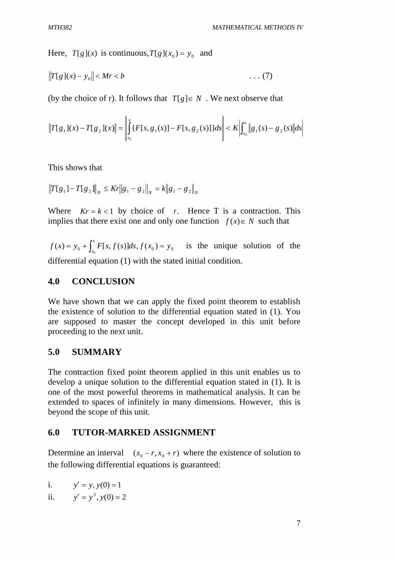
Here, )]([ xgT is continuous, 00 )]([ yxgT and
bMryxgT 0)]([ . . . (7)
(by the choice of r). It follows that NgT ][ . We next observe that
x
x
x
x
dssgsgKdssgsFsgsFxgTxgT0
0
)()()]}(,[)](,[{)]([)]([ 212121
This shows that
NNNggkggKrgTgT 212121 ][][
Where 1 kKr by choice of .r Hence T is a contraction. This implies that there exist one and only one function Nxf )( such that
000 )(,)](,[)(0
yxfdssfsFyxfx
x is the unique solution of the
differential equation (1) with the stated initial condition. 4.0 CONCLUSION We have shown that we can apply the fixed point theorem to establish the existence of solution to the differential equation stated in (1). You are supposed to master the concept developed in this unit before proceeding to the next unit. 5.0 SUMMARY The contraction fixed point theorem applied in this unit enables us to develop a unique solution to the differential equation stated in (1). It is one of the most powerful theorems in mathematical analysis. It can be extended to spaces of infinitely in many dimensions. However, this is beyond the scope of this unit. 6.0 TUTOR-MARKED ASSIGNMENT Determine an interval ),( 00 rxrx where the existence of solution to the following differential equations is guaranteed: i. 1)0(, yyy ii. 2)0(,3 yyy
MTH382 MATHEMATICAL METHODS IV
8
iii. 0)0(,2 yyxyy iv. 1)0(,1)0(, 21211 yyyyy 7.0 REFERENCES/FURTHER READING Earl, A. Coddington (nd). An Introduction to Ordinary Differential
Equations. India: Prentice-Hall. Francis, B. Hildebrand (nd). Advanced Calculus for Applications. New
Jersey: Prentice-Hall. Einar, Hille (nd). Lectures on Ordinary Differential Equations. London:
Addison-Wesley Publishing Company.
MTH382 MATHEMATICAL METHODS IV
9
UNIT 3 THE METHOD OF SUCCESSIVE APPROXIMATIONS
CONTENTS 1.0 Introduction 2.0 Objectives 3.0 Main Content 3.1 The Method of Successive Approximations 4.0 Conclusion 5.0 Summary 6.0 Tutor-Marked Assignment 7.0 References/Further Reading 1.0 INTRODUCTION The method of successive approximations is a refinement of the old device of trial and error. What has been added is control of the limiting process. We know how often the process must be repeated to bring the result with the desired limit of tolerance. The method of trial and error can be traced back to Isaac Newton who was the first to be concerned with approximate solution of algebraic equation. An infinite iteration process for the positive solution of the transcendental equation defined as:
,arctan xx 1< …….. (A) was given by Joseph Fourier in his Theorie Analytique de la Chaleur (1822). Fourier’s argument is geometrical and highly intuitive. It is not difficult to give a strict analytic convergence proof. The method of successive approximation was given by Emile Picard for differential equation in 1891. This method soon became the standard method for proving existence and uniqueness theorems for all sorts of functional equations. 2.0 OBJECTIVES At end of this unit, you should be able to: apply the method of successive approximation to determine existence and uniqueness of differential equation.
MTH382 MATHEMATICAL METHODS IV
10
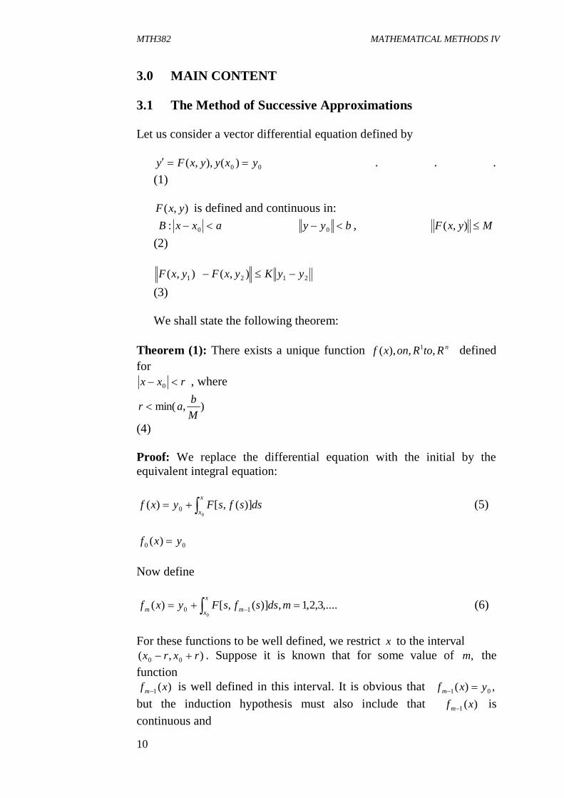
3.0 MAIN CONTENT 3.1 The Method of Successive Approximations Let us consider a vector differential equation defined by
00 )(),,( yxyyxFy . . .
(1)
),( yxF is defined and continuous in: axxB 0: byy 0 , MyxF ),( (2)
2121 ),(),( yyKyxFyxF (3)
We shall state the following theorem:
Theorem (1): There exists a unique function nRtoRonxf ,,),( 1 defined for
rxx 0 , where
),min(Mbar
(4) Proof: We replace the differential equation with the initial by the equivalent integral equation:
x
xdssfsFyxf
0
)](,[)( 0 (5)
00 )( yxf
Now define
,....3,2,1,)](,[)(0
10 mdssfsFyxfx
x mm (6)
For these functions to be well defined, we restrict x to the interval
),( 00 rxrx . Suppose it is known that for some value of ,m the function
)(1 xf m is well defined in this interval. It is obvious that ,)( 01 yxf m but the induction hypothesis must also include that )(1 xf m is continuous and
MTH382 MATHEMATICAL METHODS IV
11
.)( 01 bysf m We then see that )](,[ 1 sfsF m is well defined and continuous. Furthermore:
MsfsF m )](,[ 1 , Hence
x
x m dssfsF0
)](,[ 1 , exist as a continuous function of x and its norm does
not exceed bMrxxM 0 by the choice of .r This implies that )(xfm is also continuous and satisfies
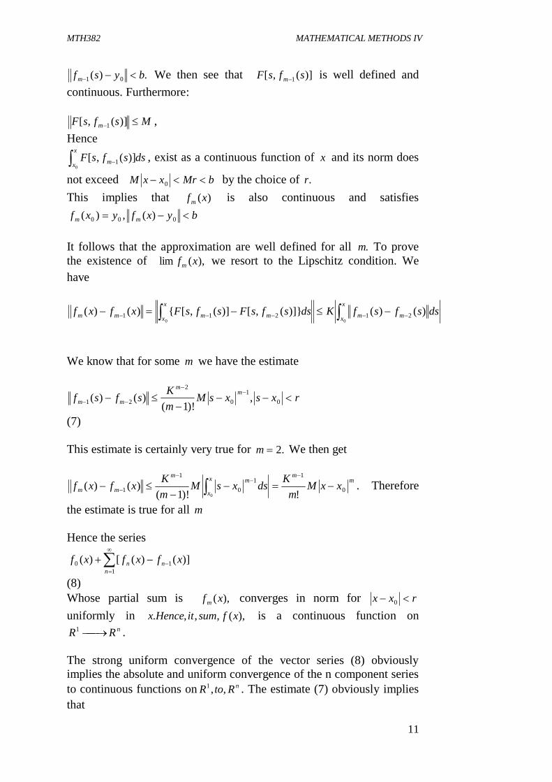
byxfyxf mm 000 )(,)( It follows that the approximation are well defined for all .m To prove the existence of ),(lim xfm we resort to the Lipschitz condition. We have
x
x mmm
x
x mmm dssfsfKdssfsFsfsFxfxf00
)()()]}(,[)](,[{)()( 21211
We know that for some m we have the estimate
rxsxsMmKsfsf m
m
mm
01
0
2
21 ,)!1(
)()(
(7) This estimate is certainly very true for .2m We then get
mmx
x
mm
mm xxMm
KdsxsMmKxfxf 0
11
0
1
1 !)!1()()(
0
. Therefore
the estimate is true for all m Hence the series
)]()([)( 11
0 xfxfxf nn
n
(8) Whose partial sum is ),(xf m converges in norm for rxx 0 uniformly in ),(,,,. xfsumitHencex is a continuous function on
nRR 1 . The strong uniform convergence of the vector series (8) obviously implies the absolute and uniform convergence of the n component series to continuous functions on nRtoR ,,1 . The estimate (7) obviously implies that
MTH382 MATHEMATICAL METHODS IV
12
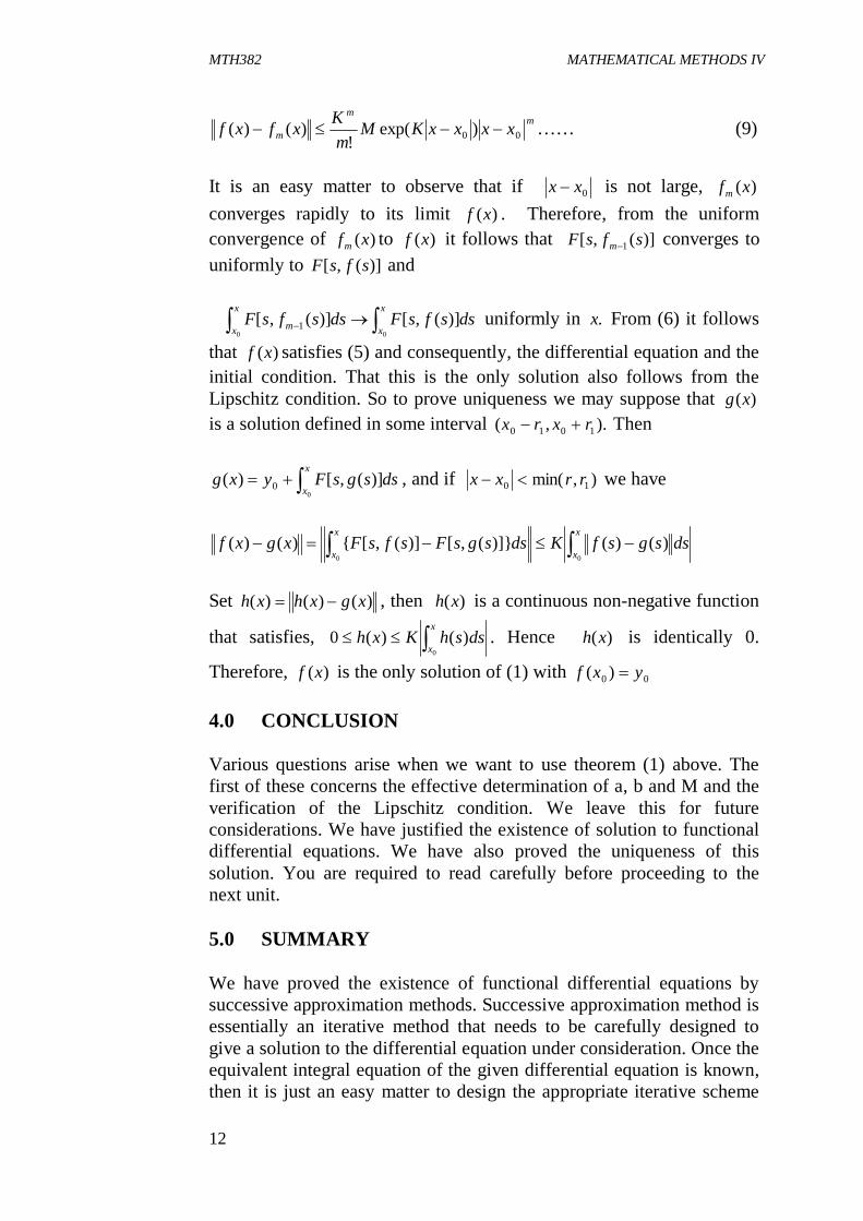
mm
m xxxxKMm
Kxfxf 00 )exp(!
)()( …… (9)
It is an easy matter to observe that if 0xx is not large, )(xfm converges rapidly to its limit )(xf . Therefore, from the uniform convergence of )(xfm to )(xf it follows that )](,[ 1 sfsF m converges to uniformly to )](,[ sfsF and
x
x
x
xm dssfsFdssfsF0 0
)](,[)](,[ 1 uniformly in .x From (6) it follows
that )(xf satisfies (5) and consequently, the differential equation and the initial condition. That this is the only solution also follows from the Lipschitz condition. So to prove uniqueness we may suppose that )(xg is a solution defined in some interval ).,( 1010 rxrx Then
x
xdssgsFyxg
0
)](,[)( 0 , and if ),min( 10 rrxx we have
x
x
x
xdssgsfKdssgsFsfsFxgxf
00
)()()]}(,[)](,[{)()(
Set )()()( xgxhxh , then )(xh is a continuous non-negative function
that satisfies, x
xdsshKxh
0
)()(0 . Hence )(xh is identically 0.
Therefore, )(xf is the only solution of (1) with 00 )( yxf 4.0 CONCLUSION Various questions arise when we want to use theorem (1) above. The first of these concerns the effective determination of a, b and M and the verification of the Lipschitz condition. We leave this for future considerations. We have justified the existence of solution to functional differential equations. We have also proved the uniqueness of this solution. You are required to read carefully before proceeding to the next unit. 5.0 SUMMARY We have proved the existence of functional differential equations by successive approximation methods. Successive approximation method is essentially an iterative method that needs to be carefully designed to give a solution to the differential equation under consideration. Once the equivalent integral equation of the given differential equation is known, then it is just an easy matter to design the appropriate iterative scheme
MTH382 MATHEMATICAL METHODS IV
13
for the equation, which will eventually converge to the solution of the equation. 6.0 TUTOR-MARKED ASSIGNMENT 1. Solve ,)0(, Cyxyy by method of successive
approximation 2. If )(xy is a solution of 0201
2 )0(,)0(,0 yyyyyxy , Show that
.)()()(0
20201 dssyssxxyyxy
x
Use the method of successive approximations to find )(sy in the special case ,0,1 0201 yy Take 1)( xf
3. The Thomas-Fermi equation defined by 2/32/1 yyx
arises in nuclear physics. Show that it has a solution of the form Cx . Show also that it can be transformed into a system to which method of successive approximation can be applied so that its solution in some interval [0,r] satisfies an initial condition of the form byay )0(,0)0( .
7.0 REFERENCES/FURTHER READING Earl, A. Coddington (nd). An Introduction to Ordinary Differential
Equations. India: Prentice-Hall. Francis, B. Hildebrand (nd). Advanced Calculus for Applications. New
Jersey: Prentice-Hall . Einar, Hille (nd). Lectures on Ordinary Differential Equations. London:
Addison-Wesley Publishing Company.
MTH382 MATHEMATICAL METHODS IV
14
MODULE 2 SPECIAL FUNCTIONS Unit 1 Special Functions Unit 2 Hyper Geometric Function Unit 3 Bessel Function UNIT 1 SPECIAL FUNCTIONS CONTENTS 1.0 Introduction 2.0 Objectives 3.0 Main Content 3.1 Special Functions
3.1.1 Gamma function 3.1.2 Beta function
3.1.3 Factorial Notation 4.0 Conclusion 5.0 Summary 6.0 Tutor-Marked Assignment 7.0 References/Further Reading 1.0 INTRODUCTION In this unit, we shall examine some special functions such as Beta function, Gamma function and Factorial function. These functions are of very useful mathematical importance in solving differential equations and other applied mathematics problems. 2.0 OBJECTIVES At the end of this unit, you should be able to: define beta function, gamma function, and factorial notations apply these functions to solve mathematical problems. 3.0 MAIN CONTENT 3.1 Special Functions Below are some of the special functions worthy of note.
MTH382 MATHEMATICAL METHODS IV
15
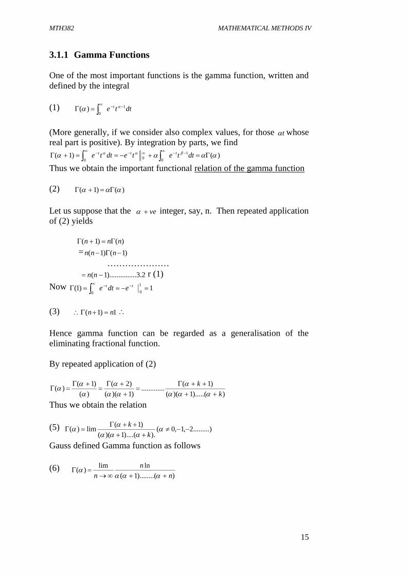
3.1.1 Gamma Functions One of the most important functions is the gamma function, written and defined by the integral (1) dtte t 1
0)(
(More generally, if we consider also complex values, for those t whose real part is positive). By integration by parts, we find
)()1( 1
000
dttetedtte ttt Thus we obtain the important functional relation of the gamma function (2) )()1( Let us suppose that the ve integer, say, n. Then repeated application of (2) yields )()1( nnn = )1()1( nnn ………………… 2.3......).........1( nn r (1) Now 1)1( 1
00
tt edte (3) 1)1( nn
Hence gamma function can be regarded as a generalisation of the eliminating fractional function. By repeated application of (2)
)).....(1)(()1(.............
)1)(()2(
)()1()(
kk
Thus we obtain the relation (5) .........)2,1,0(
).)....(1)(()1(lim)(
k
k
Gauss defined Gamma function as follows (6)
))........(1(lnlim)(
nn
n
MTH382 MATHEMATICAL METHODS IV
16
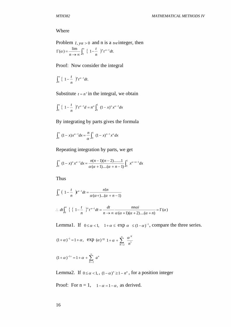
Where Problem 0, yI and n is a tve integer, then
.1lim)( 1
0dtt
nt
nnn
Proof: Now consider the integral
.1 1
0dtt
nt nn
Substitute xnt in the integral, we obtain
dxxxndtnt nnn 11
0
1
0)1(1
By integrating by parts gives the formula
dxxxndxxx nn
11
0
1
0)1()1(
Repeating integration by parts, we get
dxxn
nnndxxx nnn 11
0
1
0 )1)....(1(1).......2)(1()1(
Thus
)1)...((
11 1
0 n
nndttntn
)(
))....(2)(1(1 1
0
n
innn
dtdttntdt nn
Lemma1. If ,10 1 exp 1)1( , compare the three series.
,1)1( 1 exp )( = 1
21
n
N
N
n
Na
2
1 1)1(
Lemma2. If ,10 , nn 1)1( , for a position integer Proof: For n = 1, ,11 as derived.
MTH382 MATHEMATICAL METHODS IV
17
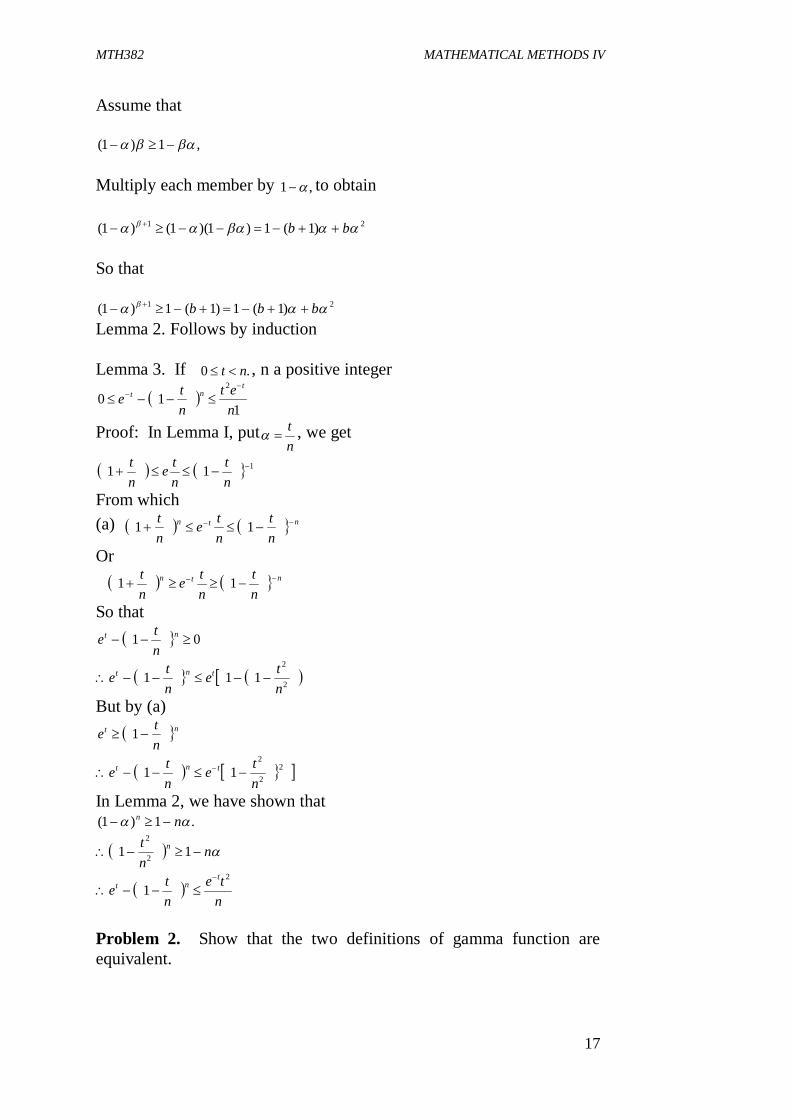
Assume that
,1)1( Multiply each member by ,1 to obtain
21 )1(1)1)(1()1( bb So that
21 )1(1)1(1)1( bbb Lemma 2. Follows by induction Lemma 3. If .0 nt , n a positive integer
1
102
net
nte
tnt
Proof: In Lemma I, putnt
, we get
111 nt
nte
nt
From which (a) ntn
nt
nte
nt 11
Or ntn
nt
nte
nt 11
So that 01 nt
nte
2
2
111nte
nte tnt
But by (a) nt
nte 1
22
2
11nte
nte tnt
In Lemma 2, we have shown that .1)1( nn
nnt n 11 2
2
nte
nte
tnt
2
1
Problem 2. Show that the two definitions of gamma function are equivalent.
MTH382 MATHEMATICAL METHODS IV
18
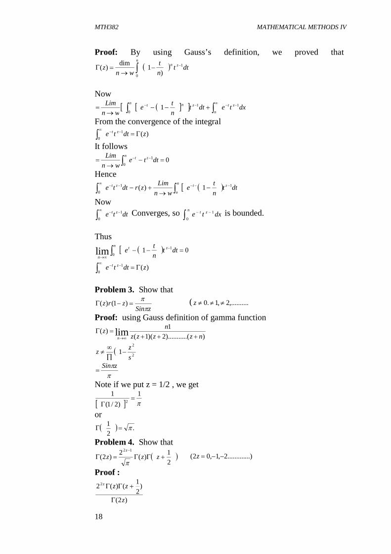
Proof: By using Gauss’s definition, we proved that
dttnt
wnz zn
n1
0 )1dim)(
Now
dxtedttnte
wnLim zt
n
zntn 11
01
From the convergence of the integral )(1
0zdtte zt
It follows
01
0
dtte
wnLim ztn
Hence dtt
nte
wnLimzrdtte ztn
o
zt 11
01)(
Now dtte zt 1
0
Converges, so dxte ztn 1
0
is bounded. Thus
01 1
0lim
dtt
nte ztn
n
)(1
0zdtte zt
Problem 3. Show that
zSinzrz
)1()( ( .,.........2,1.0 z
Proof: using Gauss definition of gamma function
)..().........2)(1(1)( lim nzzzz
nzn
2
2
1szz
zSin
Note if we put z = 1/2 , we get
1
)2/1(1
2
or .
21
Problem 4. Show that
21)(2)2(
12
zzzz
...)..........2,1,02( z
Proof :
)2(
)21()(2 2
z
zzz

MTH382 MATHEMATICAL METHODS IV
19
21(
....232(
21)()...(1(
212 22
lim
nzznzzz
ninnin zz
n
nnni n
n 1)2(2)( 122
lim
The last quantity is independent of z and must be finite since the left side exists.
Az
zzz
)2(
)21()(2 2
Put z = ½ We have
2A
21()(2
)2(
12
zzz
z
3.1.2 Beta-Function We define Beta-function ),( qpB by (1) ),( qpB 0)(,0)(,,1( 111
0 qRcRdxtt qp
Another useful form of this function can be obtained by putting t =
,2Sint thus arriving at (2) 0)(,0)(,2),( 1212
0 qRpRdCosSinqpB qpl
Next we establish the relation between gamma and beta-functions Problem: If .0)(,0)( qRpR Then
)()()(),(
qprqrprqpB
Proof: duuedtteqrpr quPt 1
0
1
0)()(
Substituting 22 yandUxt it gives dyyedxxeqrpr qypx 122
0
122
04)()(
dxdyyxyxqrpr qp 121222
00)exp(4)()(

MTH382 MATHEMATICAL METHODS IV
20
Next, turn to polar co-ordinate for the iterated integration over the first quadrant in xy-plan.
drdSinCosrqrpr qpqp 12122222200
)2exp(4)()(
dSinCosdrrr qplqp 12121222
02)exp(2
Take ,212 andr t we obtain
dCosSindtteqrpr qpqpt 121221
0
1
02exp()()(
= ),()( qpBqpr
)()()(),(
qprqrprqpB
.
3.1.3 Factorial Notations (1) )1()( k
lln
n
)1)......(1( n 0,1)( 0 The function 0)( is called the factorial notation Problem: Show that
nnn
n 21
22)( 2
2
Proof:- )12)......(3)(2)(1)(()( 2 nn )12).......(3)(1()22)......(2)(( nn =
222..........
24
22
222 nn
12
1............2
12
1
n
nnn
21
22 2
Similarly, we can show that
nnkn
kn kk
kkK 1...........1)(
Problem: show that
)()()(
nn
MTH382 MATHEMATICAL METHODS IV
21
Proof: )().........2)(1()( nnn )()1().........1)(( n )()()( nn
)()()(
nn
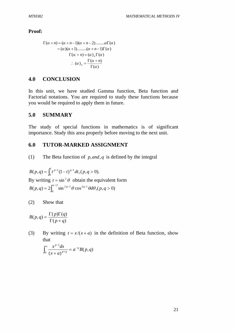
4.0 CONCLUSION In this unit, we have studied Gamma function, Beta function and Factorial notations. You are required to study these functions because you would be required to apply them in future. 5.0 SUMMARY The study of special functions in mathematics is of significant importance. Study this area properly before moving to the next unit. 6.0 TUTOR-MARKED ASSIGNMENT (1) The Beta function of qandp ,, is defined by the integral
).0,(,)1(),( 11
0
1 qpdtttqpB qp
By writing 2sint obtain the equivalent form )0,(,cossin2),(
2/
0
1212 qpdqpB qp
(2) Show that
),( qpB)()()(
qpqp
(3) By writing )/( axxt in the definition of Beta function, show
that
),()(0
1
qpBaax
dxx qqp
p

MTH382 MATHEMATICAL METHODS IV
22
7.0 REFERENCES/FURTHER READING Earl, A. Coddington (nd). An Introduction to Ordinary Differential
Equations. India: Prentice-Hall. Francis, B. Hildebrand (nd). Advanced Calculus for Applications. New
Jersey: Prentice-Hall. Einar, Hille (nd). Lectures on Ordinary Differential Equations. London:
Addison-Wesley Publishing Company.
MTH382 MATHEMATICAL METHODS IV
23
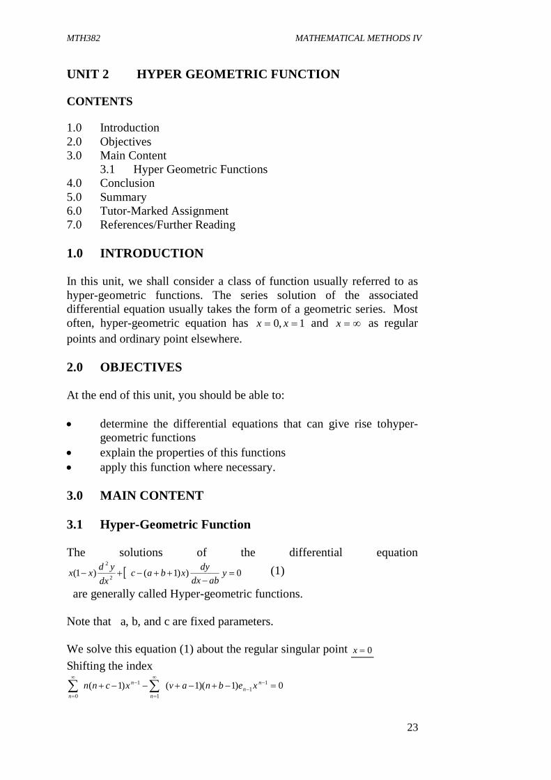
UNIT 2 HYPER GEOMETRIC FUNCTION CONTENTS 1.0 Introduction 2.0 Objectives 3.0 Main Content 3.1 Hyper Geometric Functions 4.0 Conclusion 5.0 Summary 6.0 Tutor-Marked Assignment 7.0 References/Further Reading 1.0 INTRODUCTION In this unit, we shall consider a class of function usually referred to as hyper-geometric functions. The series solution of the associated differential equation usually takes the form of a geometric series. Most often, hyper-geometric equation has 1,0 xx and x as regular points and ordinary point elsewhere. 2.0 OBJECTIVES At the end of this unit, you should be able to: determine the differential equations that can give rise tohyper-
geometric functions explain the properties of this functions apply this function where necessary. 3.0 MAIN CONTENT 3.1 Hyper-Geometric Function The solutions of the differential equation
0))1()1( 2
2
yabdx
dyxbacdx
ydxx (1)
are generally called Hyper-geometric functions. Note that a, b, and c are fixed parameters. We solve this equation (1) about the regular singular point 0x Shifting the index
0)1)(1()1( 11
1
1
0
n
nn
n
n
xebnavxcnn
MTH382 MATHEMATICAL METHODS IV
24
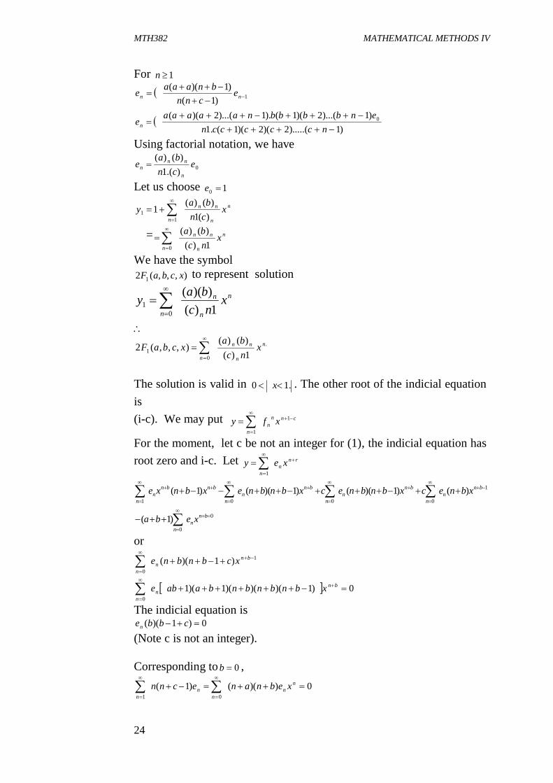
For 1n 1)1(
)1)((
nn e
cnnbnaaae
)1).....(2)(2)(1(.1
)1)...(2)(1().1)...(2)(( 0
ncccccn
enbbbbnaaaaaen
Using factorial notation, we have
0).(1)()(
ecnba
en
nnn
Let us choose 10 e n
n
nn
nx
cnba
y)(1)()(
11
1
= n
n
nn
nx
ncba
1)()()(
0
We have the symbol ),,,(2 1 xcbaF to represent solution
n
n
n
nx
ncbay
1)())((
01
The solution is valid in .10 x . The other root of the indicial equation is (i-c). We may put cnn
nn
xfy
1
1
For the moment, let c be not an integer for (1), the indicial equation has root zero and i-c. Let rn
nn
xey
1
0
0
1
0001
)1(
)()1)(()1)(()1(
bnn
n
bnn
n
bnn
n
bnn
n
bnbnn
n
xeba
xbnecxbnbnecxbnbnexbnxe
or 1
0
)1)((
bnn
n
xcbnbne
0)1)()()(1)(10
bn
nn
xbnbnbnbaabe
The indicial equation is 0)1)(( cbben
(Note c is not an integer). Corresponding to 0b ,
0))(()1(01
nn
nn
n
xebnanecnn
.
01 1)(
)()(),,,(2 n
n
nn
nx
ncba
xcbaF
MTH382 MATHEMATICAL METHODS IV
25
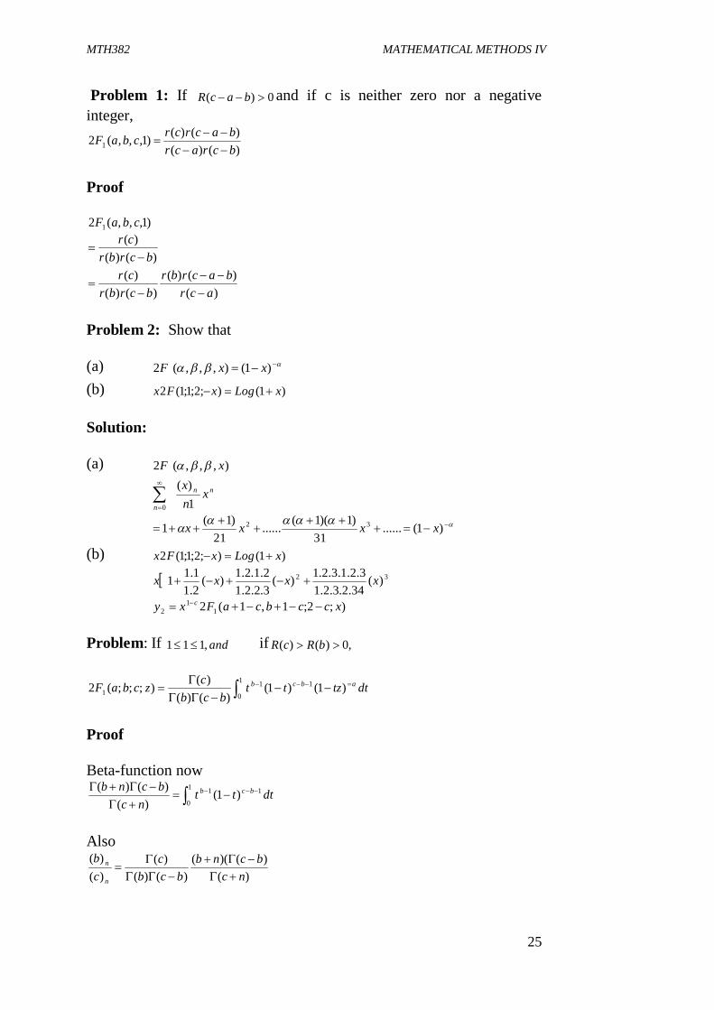
Problem 1: If 0)( bacR and if c is neither zero nor a negative integer,
)()()()()1,,,(2 1 bcracr
bacrcrcbaF
Proof
)1,,,(2 1 cbaF
)()()(
bcrbrcr
)()()(
)()()(
acrbacrbr
bcrbrcr
Problem 2: Show that (a) )1(),,,(2 xxF (b) )1();2;1;1(2 xLogxFx Solution: (a) ),,,(2 xF
nn
n
xnx1)(
0
)1(......
31)1)(1(......
21)1(1 32 xxxx
(b) )1();2;1;1(2 xLogxFx 32 )(
34.2.3.2.13.2.1.3.2.1)(
3.2.2.12.1.2.1)(
2.11.11 xxxx
);2;1,1(2 11
2 xccbcaFxy c Problem: If and,111 if ,0)()( bRcR
dttzttbcb
czcbaF abcb
)1()1(
)()()();;;(2 111
01
Proof Beta-function now
dtttnc
bcnb bcb 111
0)1(
)()()(
Also
)()()((
)()()(
)()(
ncbcnb
bcbc
cb
n
n
MTH382 MATHEMATICAL METHODS IV
26
Thus
)()()();;;(2 1 bcb
czcbaF
dtttN
za bcnbn
n
111
00
)1(1
)(
1))((
)()()(
0
11
0 ndtztat
bcbc n
n
b
dtzttbcb
c ab )1()()(
)( 111
0
Where
1)1)(1)...(1)(()1(
0 nynz
nn
n
a
1)1)...(1(
0 nyn n
n
1)1)...(1(
0 nyna n
n
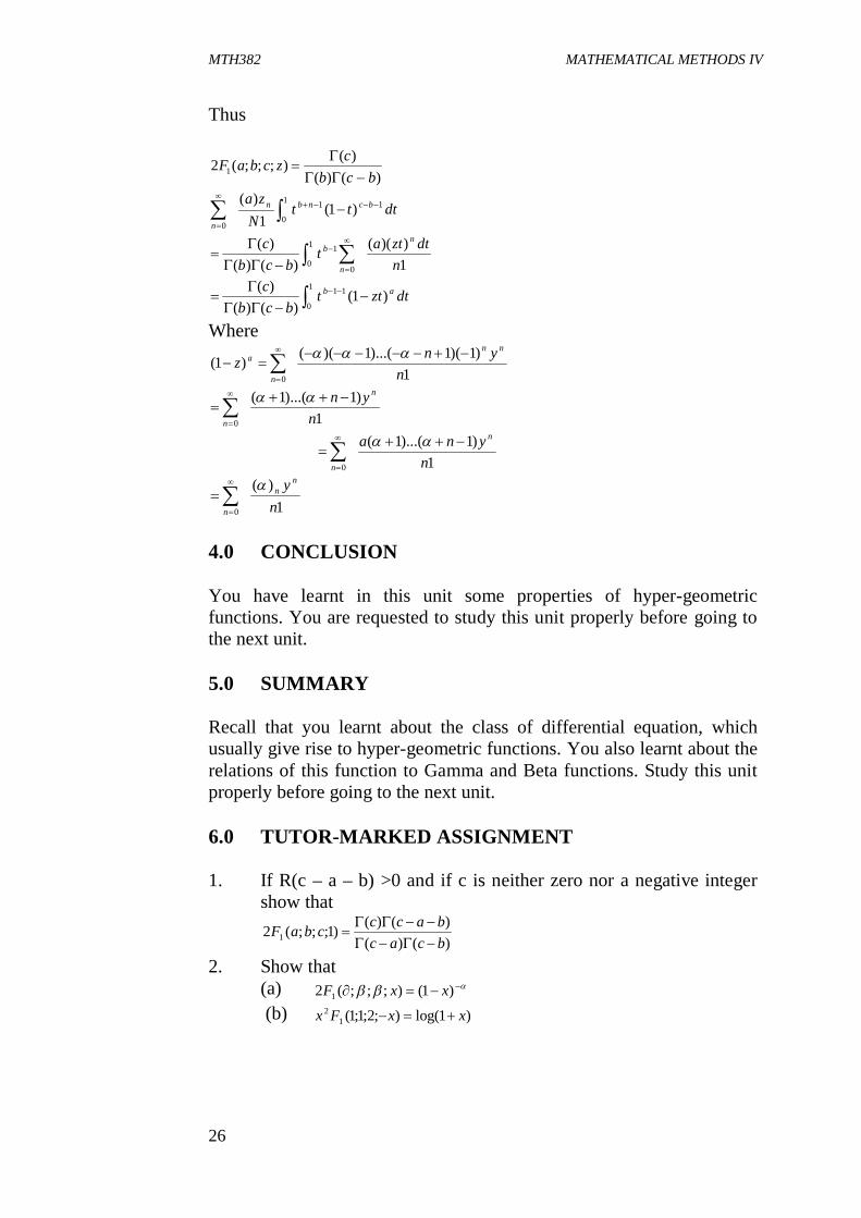
4.0 CONCLUSION You have learnt in this unit some properties of hyper-geometric functions. You are requested to study this unit properly before going to the next unit. 5.0 SUMMARY Recall that you learnt about the class of differential equation, which usually give rise to hyper-geometric functions. You also learnt about the relations of this function to Gamma and Beta functions. Study this unit properly before going to the next unit. 6.0 TUTOR-MARKED ASSIGNMENT 1. If R(c – a – b) >0 and if c is neither zero nor a negative integer
show that
)()()()()1;;;(2 1 bcac
bacccbaF
2. Show that (a) )1();;;(2 1 xxF (b) )1log();2;1;1(1
2 xxFx
1)(
0 ny n
n
n
MTH382 MATHEMATICAL METHODS IV
27
7.0 REFERENCES/FURTHER READING Earl, A. Coddington (nd). An Introduction to Ordinary Differential
Equations. India: Prentice-Hall. Francis, B. Hildebrand (nd). Advanced Calculus for Applications. New
Jersey: Prentice-Hall. Einar, Hille (nd). Lectures on Ordinary Differential Equations. London:
Addison-Wesley Publishing Company.
MTH382 MATHEMATICAL METHODS IV
28
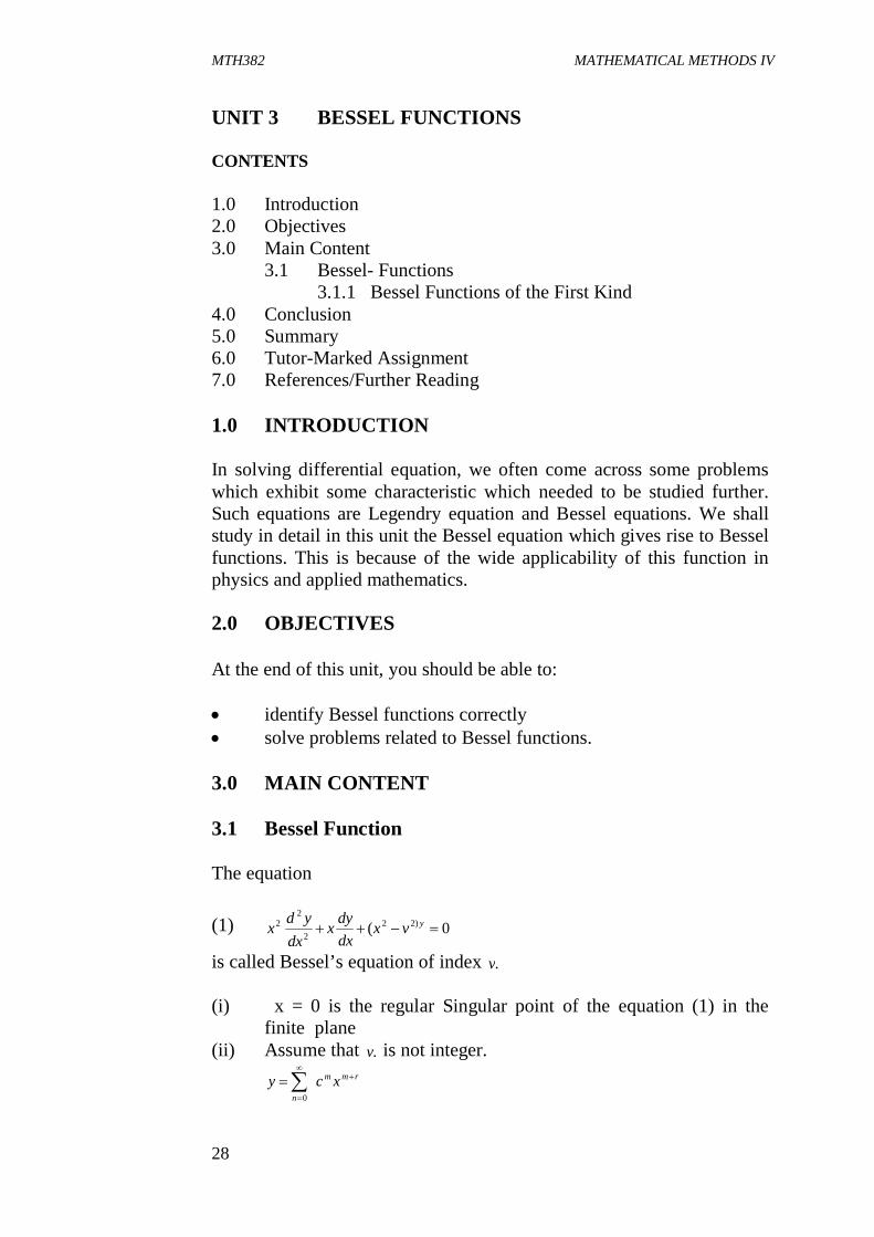
UNIT 3 BESSEL FUNCTIONS CONTENTS 1.0 Introduction 2.0 Objectives 3.0 Main Content 3.1 Bessel- Functions 3.1.1 Bessel Functions of the First Kind 4.0 Conclusion 5.0 Summary 6.0 Tutor-Marked Assignment 7.0 References/Further Reading 1.0 INTRODUCTION In solving differential equation, we often come across some problems which exhibit some characteristic which needed to be studied further. Such equations are Legendry equation and Bessel equations. We shall study in detail in this unit the Bessel equation which gives rise to Bessel functions. This is because of the wide applicability of this function in physics and applied mathematics. 2.0 OBJECTIVES At the end of this unit, you should be able to: identify Bessel functions correctly solve problems related to Bessel functions. 3.0 MAIN CONTENT 3.1 Bessel Function The equation (1) 0( )22
2
22 yvx
dxdyx
dxydx
is called Bessel’s equation of index .v (i) x = 0 is the regular Singular point of the equation (1) in the
finite plane (ii) Assume that .v is not integer. rmm
n
xcy
0

MTH382 MATHEMATICAL METHODS IV
29
Substituting this expression and its first and second derivatives into Bessel equation, we obtain
0)()1)((0
22
000
zm
mm
rmm
m
rmm
m
rmm
n
xcVxcxcrmxczmzm
(a) 0)1( 02
00 cvrccrr )0( m (b) 0)1())(1( 1
211 cvcrcrr )1( m
(c) 0)1)(( 2 mmm vcccrmrm ,....3,2( m Now ,00 c thus the indicial equation from (a) 0))(( vrvr The roots are 0 vvr vr 22 21 ,0v egerv int v2 integral multiply of v2 , i.e. v is zero or ve integer Now we obtain the solution corresponding to the value .vr From (b) we obtain 01 c (c) can be written
0))(( 2 mm ccvrmvrm Since 01 c , it follows that .0.......753 ccc Thus we put replace m by
.2m 0)2)(2( 22 mm ccvrmvrm
Now vr
0)2)(22( 222 mm ccmvm
mmvc
c zmm )(22
22
(but v is not integer) ,....)2,1( m
Assume
)1(1
20
vrvc
)2(1121
)1(2 220
2
vrvc
c v
)3(2121
)2(2.2 222
4
vrvc
c v
)1(12)1(
22
mvrm
cvm
m
m
Thus, the solution is
)(12)1(
2
2
0 mvrmxy vm
mm
m

MTH382 MATHEMATICAL METHODS IV
30
We denote this solution by the notation
1)1(2
)1()(2
2
0 mvmr
xxxJ vm
mm
m
vv
(2)
)(xJv is called the Bessel Function of the first kind of order .v
By Ratio test we know that the series converges for all values of x Replacing v by v , we have
1)11(2
)1()(2
2
0 mvmr
xxxJ vm
mm
m
vv
(3)
(2) and (3) are the independent solutions. Thus )()( 21 xJcxJcy vv (i) If ,0v then the solution )(xJ v and )(xJ v are identical. One can
verify from (2) and (3) (ii) If v is ve integer, then the second solution )(xJ v is not
independent of )(xJ v Say nv then the factor
11
1(1
nmnmr
in (3) is zero
When nm hence (3) is equivalent to Replace m by nm in 5, we get change the index
11
2)1(
)(
2
0 nmm
x
xJ
nmmm
mv
(6)
From (2), when nv integer, thus
1,12
)1()(
2
0 nmm
x
xxJ
nmm
m
vv
(7)
From (6) and (7), we get )()1()( xJxJ n
nv (8)
Further properties of Bessel functions of first bind From (2)
1)1(2
)1()(2
22
0 mvmr
xxJx vm
vmm
mv
v
Now we use the formula )1()( rr
1)(2)1(
2
122
0
1
mvmrxxx vm
vmm
m
vv
MTH382 MATHEMATICAL METHODS IV
31
)(12)1(
12
2
0
1
vmrmxxx vm
mm
m
vv
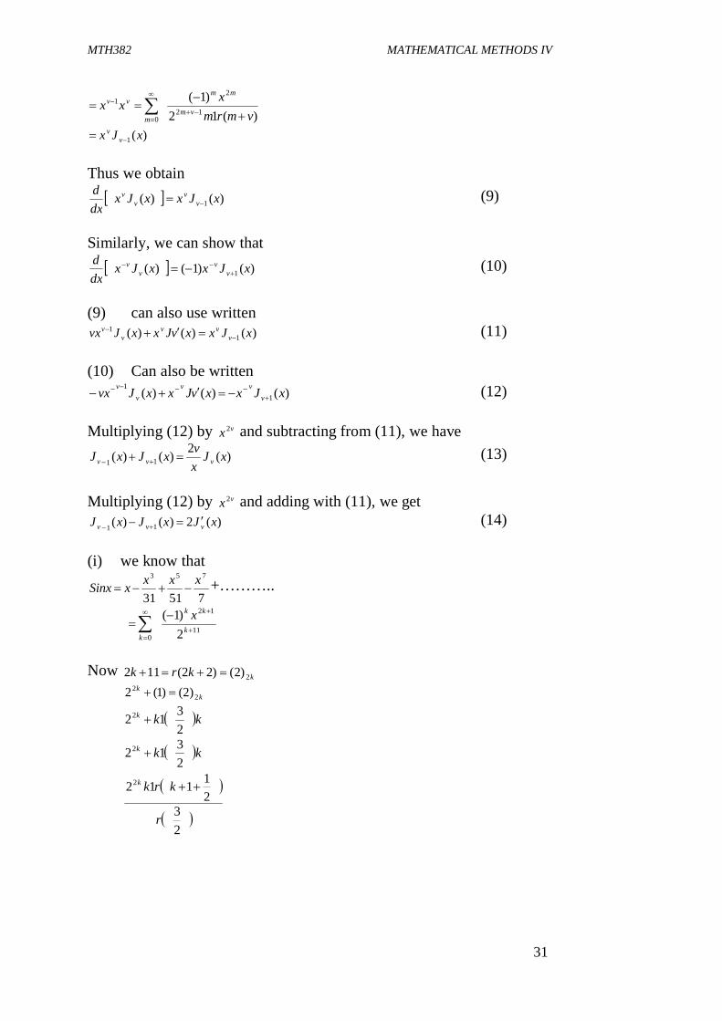
)(1 xJx vv
Thus we obtain
)()( 1 xJxxJxdxd
vv
vv
(9)
Similarly, we can show that
)()1()( 1 xJxxJxdxd
vv
vv
(10)
(9) can also use written
)()()( 11 xJxxvJxxJvx v
vvv
v
(11) (10) Can also be written
)()()( 11 xJxxvJxxJvx v
vvv
v
(12) Multiplying (12) by vx 2 and subtracting from (11), we have
)(2)()( 11 xJxvxJxJ vvv
(13)
Multiplying (12) by vx 2 and adding with (11), we get
)(2)()( 11 xJxJxJ vvv (14)
(i) we know that
75131
753 xxxxSinx +………..
11
12
0 2)1(
k
kk
k
x
Now kkrk 2)2()22(112 k
k2
2 )2()1(2
kkk
23122
kkk
23122
23
211122
r
krkk

MTH382 MATHEMATICAL METHODS IV
32
But 21
21
21
23
rr
21112
112
12
krkk
k
211(12
)1(12
12
0
krk
xSinxk
kk
k
(15) If we take
21
V , then from (2), we have
)21(2
)1(21)(
21
2
2
0
kr
xxxJvk
kk
k
(16) From (15) and (16), we have
xx
xJv sin)2)(
In similar manner, by considering the expansion
!)2(
)1(cos2
0 nzz
n
n
, we obtain
The formula
xx
xJ v cos)2)(2
Problems (i) )(1)( 1 xJxJ o (ii) )22(
41
2 nnnn JJJvJ
(iii) )(1)()( 101 xJx
xJxJ
(iv) )(2)()41()( 0122 xJx
xJx
xJ
(v) )()1()()( 11
1 xdxJxnmxJxdxxJx nm
nm
nm
Solution
dxxJxxdxxJx nnnm
nm )]([)( 11
dxxJxdxdx n
nnm )]([ 111
MTH382 MATHEMATICAL METHODS IV
33
Integrating by parts, we have dxxJxnmxJx n
mn
m )()1()( 11
1
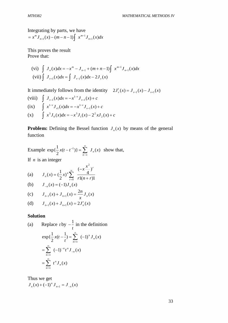
This proves the result Prove that: (vi) dxxJxnmJxdxxJ n
mn
mn )()1()( 1
11
(vii) )(2)()( 11 xJdxxJdxxJ vvv
It immediately follows from the identity )()()(2 11 xJxJxJ vvv (viii) cxJxdxxJ v
vv
)()( 1
11
(ix) cxJxdxxJx vv
vv
)()( 11
11
(x) cxxJxJxdxxJx )(2)()( 22
13
03
Problem: Defining the Bessel function )(xJ n by means of the general function
Example )()}(21exp{ 1 xJttx n
n
show that,
If n is an integer
(a) 1)(1
)4
()
21()(
2
0 rnr
xxxxJ
r
r
nn
(b) )()1()( xJxJ nn
(c) )(2)()( 11 xJxnxJxJ nnn
(d) )(2)()( 11 xJxJxJ nnn Solution
(a) Replace t by t1
in the definition
)()1()1(21exp{ xJ
ttx n
n
n
)()1( xJt nnn
n
)(xJt nn
n
Thus we get
)()1()( 1 xJJxJ nnn
n

MTH382 MATHEMATICAL METHODS IV
34
The exponential on the left can be expressed as a product of two exponential
nn
ntx
nttx
)2
(1
1)(2
exp[0
1
mm
mtx
m
)2
(1
10
Every product of a term of the first series by a term of the second contains a factor mnt . Let’s associate with each term of the second series the term of the first series corresponding to )0( pmpn . The product contains the factors pt . Therefore the series expansions of the coefficient )(xj p with ve p follow. By associating with each term of the first series the term of the second series which corresponds to 0( pnpm , the product contains now the factor pt . Thus )(xj p is obtained. Problem: Prove that
0)coscos(21)(
2
0dzzjo
Proof: We know that
nn
ntzjttz )()(
2exp[ 1
Put
iiet , take real parts of both sides and integrate between 0 and 2 ………..
)tan(cos)()]2
exp[
nn
n
ii izjieiez
)tan(cos)()(1
0
nn
nizjzj
)tan(cos)(1
nn
nizj
"")()cosexp[ 0 zJz Problem: Prove that
zzdzJ sincos)cos(0
20
MTH382 MATHEMATICAL METHODS IV
35
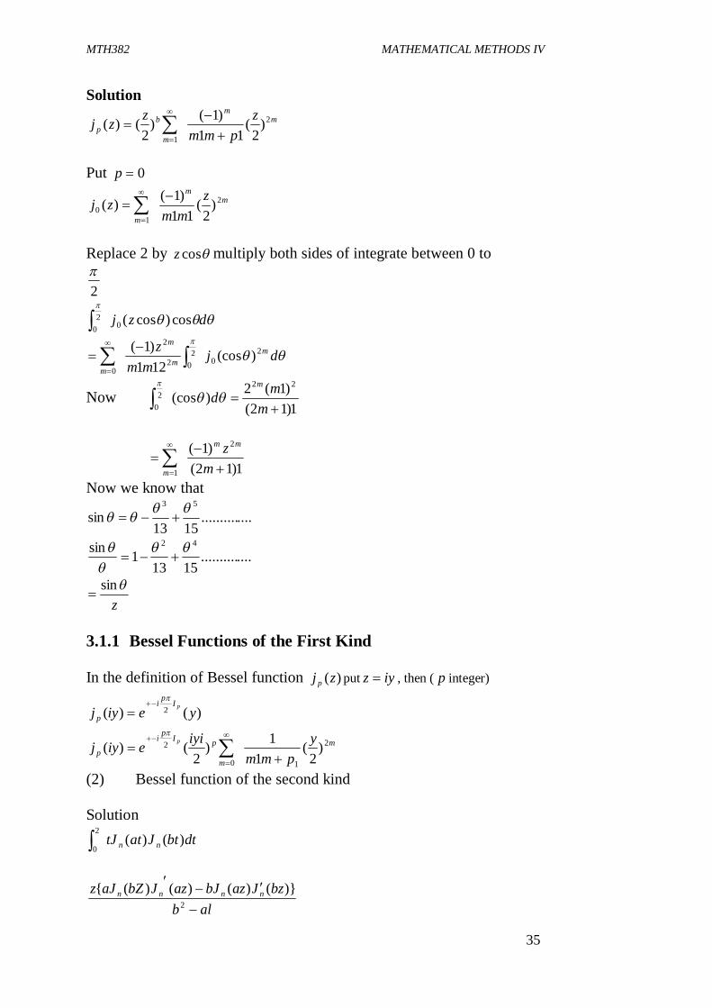
Solution m
m
m
bp
zpmm
zzj 2
1)
2(
11)1()
2()(
Put 0p
mm
m
zmm
zj 2
10 )
2(
11)1()(
Replace 2 by cosz multiply both sides of integrate between 0 to
2
dzj cos)cos(02
0
djmm
z mm
m
m
20
202
2
0)(cos
121)1(
Now 1)12(
)1(2)(cos22
20
mmd
m
1)12(
)1( 2
1
mz mm
m
Now we know that
..............1513
sin53
..............1513
1sin 42
zsin
3.1.1 Bessel Functions of the First Kind In the definition of Bessel function )(zj p put iyz , then ( p integer)
)()( 2 yeiyj pIpi
p
m
m
pIpi
py
pmmiyieiyj p 2
10
2 )2
(1
1)2
()(
(2) Bessel function of the second kind Solution
dtbtJattJ nn )()(2
0
albbzJazbJazJbZaJz nnnn
2
)}()()()({
MTH382 MATHEMATICAL METHODS IV
36
Solution
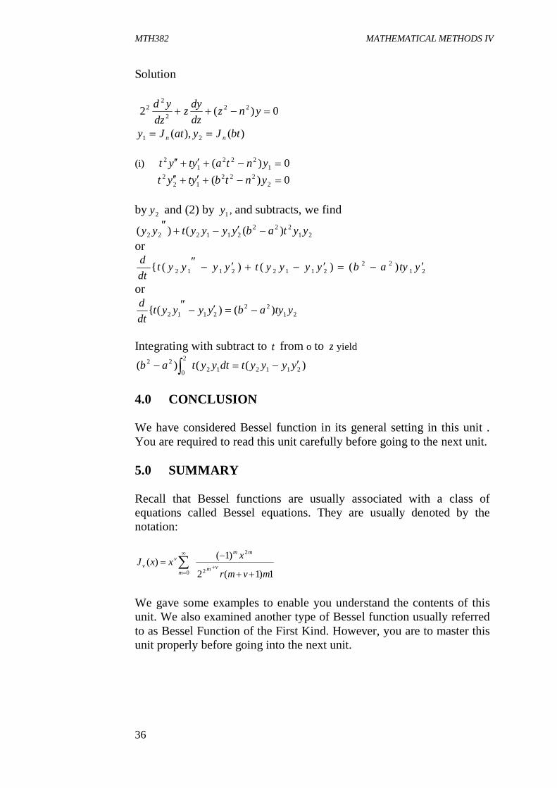
0)(2 222
22 ynz
dzdyz
dzyd
)(),( 21 btJyatJy nn (i) 0)( 1
2221
2 yntaytyt 0)( 2
22212
2 yntbytyt by 2y and (2) by 1y , and subtracts, we find
21222
211222 )(()( yytabyyyytyy or
2122
21122112 )()()({ ytyabyyyytyyyytdtd
or
2122
2112 )()({ ytyabyyyytdtd
Integrating with subtract to t from o to z yield
)(()( 211212
2
0
22 yyyytdtyytab
4.0 CONCLUSION We have considered Bessel function in its general setting in this unit . You are required to read this unit carefully before going to the next unit. 5.0 SUMMARY Recall that Bessel functions are usually associated with a class of equations called Bessel equations. They are usually denoted by the notation:
1)1(2
)1()(2
2
0 mvmr
xxxJ vm
mm
m
vv
We gave some examples to enable you understand the contents of this unit. We also examined another type of Bessel function usually referred to as Bessel Function of the First Kind. However, you are to master this unit properly before going into the next unit.

MTH382 MATHEMATICAL METHODS IV
37
6.0 TUTOR-MARKED ASSIGNMENT 1. Given that
)()1(
2 xJre nn
nrrx
Deduce that )]()([2
)()1( 21 xJxJxxJn nnn
2. Obtain the general solution of each of the following equations in terms of Bessel functions, or if possible in terms of elementary functions.
(a) 032
2
xydxdy
dxydx (b) 04 3
2
2
yxdxdy
dxydx (c) 02
2
24 ya
dxydx
7.0 REFERENCES/FURTHER READING Earl, A. Coddington (nd). An Introduction to Ordinary Differential
Equations. India: Prentice-Hall. Einar, Hille (nd). Lectures on Ordinary Differential Equations. London:
Addison – Wesley Publishing Company. Francis, B. Hildebrand (nd). Advanced Calculus for Applications. New
Jersey: Prentice-Hall.
MTH382 MATHEMATICAL METHODS IV
38
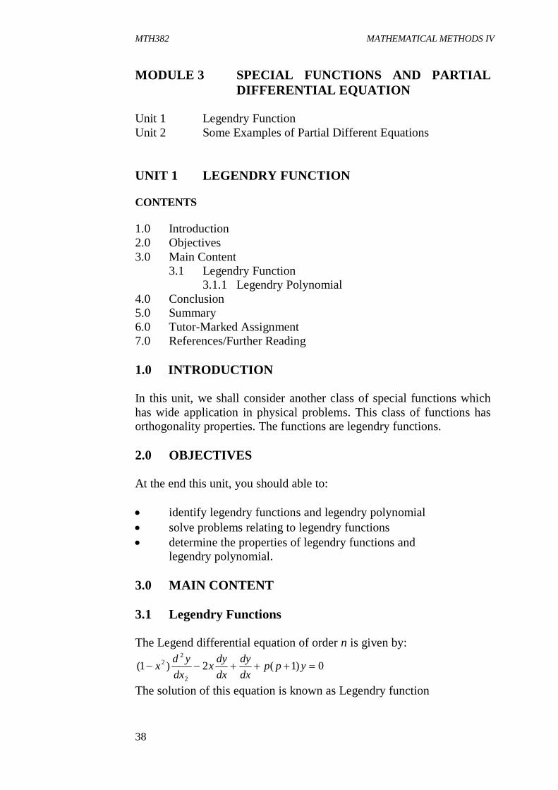
MODULE 3 SPECIAL FUNCTIONS AND PARTIAL DIFFERENTIAL EQUATION
Unit 1 Legendry Function Unit 2 Some Examples of Partial Different Equations UNIT 1 LEGENDRY FUNCTION CONTENTS 1.0 Introduction 2.0 Objectives 3.0 Main Content 3.1 Legendry Function 3.1.1 Legendry Polynomial 4.0 Conclusion 5.0 Summary 6.0 Tutor-Marked Assignment 7.0 References/Further Reading 1.0 INTRODUCTION In this unit, we shall consider another class of special functions which has wide application in physical problems. This class of functions has orthogonality properties. The functions are legendry functions. 2.0 OBJECTIVES At the end this unit, you should able to: identify legendry functions and legendry polynomial solve problems relating to legendry functions determine the properties of legendry functions and legendry polynomial. 3.0 MAIN CONTENT 3.1 Legendry Functions The Legend differential equation of order n is given by:
0)1(2)1(2
22 ypp
dxdy
dxdyx
dxydx
The solution of this equation is known as Legendry function
MTH382 MATHEMATICAL METHODS IV
39
0)1(2)1()1(0
1
1
2
2
2
nn
n
nn
n
nn
nxcppnxcxxnncx
0)]}1()1([)1)(2{( 22
n
nnn
xppnnccnn
Recurrence relation
)()1)(2( 2222 ppnnccnn n (2)
Thus
nn cnn
npnpc)1)(2(
)1)((2
Therefore
ocppc21
)1(2
ocppc
21)1(
2
ocppc31
)1(3
24 21)3)(2( cPppc
01.4)3)(1)()(2( cPppp
25 4.5)4)(3( cPpc
etccPppp01.4
)4)(2)(1)(3(
41
)3)(1()2(21
)1(142
1xppppxppy
51
)4)(2)(1)(3(31
)2)(1(53
2xppppxppxy
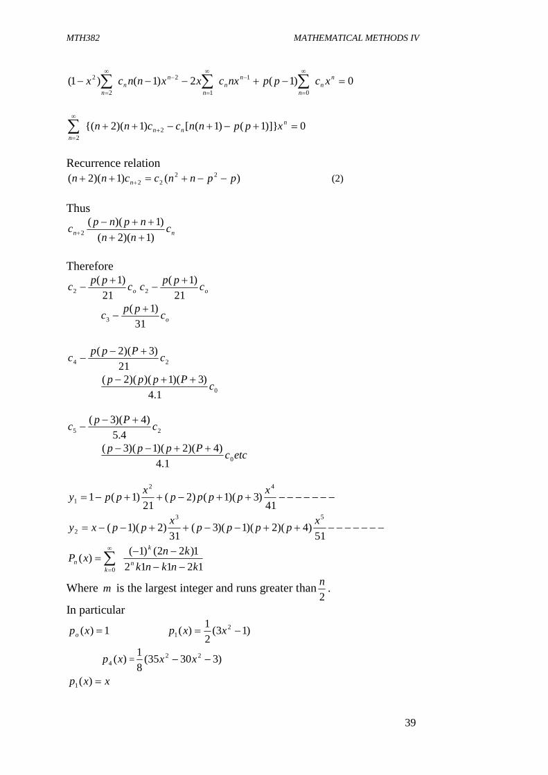
121121)22()1()(
0 knknkknxP n
k
kn
Where m is the largest integer and runs greater than2n .
In particular
1)( xpo )13(21)( 2
1 xxp
)(4 xp = )33035(81 22 xx
xxp )(1
MTH382 MATHEMATICAL METHODS IV
40
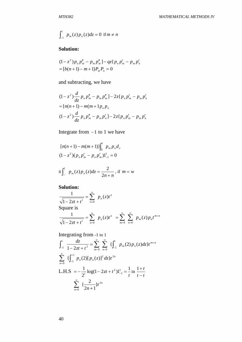
0)()(1
1 dzzpzp nm if nm
Solution:
nmmnmmmn ppppqzppppz {])1( 2 0)1)1([ nm PPmnb
and subtracting, we have
nmmnmmmn ppppzppppdzdz {2])1( 2
nn ppmmnn 1()1([
nmmnnmmn ppppzppppdzdz {2])1( 2
Integrate from 1 to 1 we have znm dppmmnn
1
0)]1()1([
01))(1( 11
2 mnmn ppppz
iinn
dzzpzp nm 2
2)()(1
`, if wm
Solution:
nn
nt
tzptzt
)(211
0
Square is n
nn
ttzp
tzt)(
211
0
nmnm
nmtpzp
)(
00
Integrating from -1 to 1
nmnm
nmtdzzpp
tztdz
})()2({
211
100
2
1
1
nnn
ntdzzpp 221
10
})]()[2({
L.H.S t
tztt
11)21log(21 1
12 in
ttt
1
n
nt
n2
0}
122{
MTH382 MATHEMATICAL METHODS IV
41
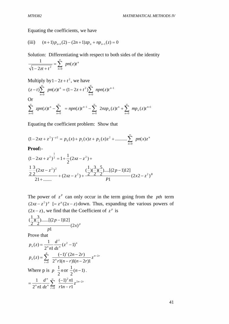
Equating the coefficients, we have (iii) 0)()12()2()1( 11 znpzpnpn nnn Solution: Differentiating with respect to both sides of the identity
n
ntzpn
tzt)(
211
02
Multiply by 221 tz , we have
1
0
2
0)()21()()(
n
n
n
ntznpntztzpntz
Or 1
00
1
00)()(2)()(
n
nn
nn
n
n
n
n
ntzmptznzptznpntzzpn
Equating the coefficient problem: Show that
..........)()()()21( 2210
22 zxpzxpxpzxz y n
nzxpn )(
0
Proof:-
)2(211)21( 22
12 zxzzxz
BzxP
pzxz
zxz)22(
1
]12)12)....[(25)(
23)(
21(
)2(.......21
)2(23
21
22
22
The power of Pz can only occur in the term going from the pth term
pzxz )2( 2 )2([ zxz p down. Thus, expanding the various powers of )2( zx , we find that the Coefficient of pz is
pxp
p)2(
1
]12)12)......[(23)(
21(
Prove that n
nnn zdzd
nzp )1(
121)( 2
rnn
rp
rn z
rnrnrrnzp 2
0 1)2(1)(12)22()1()(
Where p is p n21 or )1(
21
n .
rn
rn
n
n zrnrn
dzd
n22
2
0 111)1(
121
MTH382 MATHEMATICAL METHODS IV
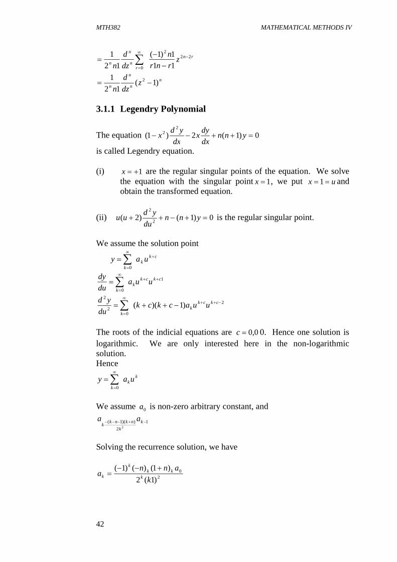
42
rn
rn
n
n zrnrn
dzd
n22
2
0 111)1(
121
nn
n
n zdzd
n)1(
121 2
3.1.1 Legendry Polynomial
The equation 0)1(2)1(2
2 ynndxdyx
dxydx
is called Legendry equation. (i) 1x are the regular singular points of the equation. We solve
the equation with the singular point 1x , we put ux 1 and obtain the transformed equation.
(ii) 0)1()2( 2
2
ynndu
yduu is the regular singular point.
We assume the solution point
ckk
kuay
0
1
0
ckckk
kuua
dudy
2
02
2
)1)((
ckckk
kuuackck
duyd
The roots of the indicial equations are 0,0c 0. Hence one solution is logarithmic. We are only interested here in the non-logarithmic solution. Hence
kk
kuay
0
We assume 0a is non-zero arbitrary constant, and
12
))(1(2
kk
nknkkaa
Solving the recurrence solution, we have
20
)1(2)1()()1(
kann
a kkk
k
k
MTH382 MATHEMATICAL METHODS IV
43
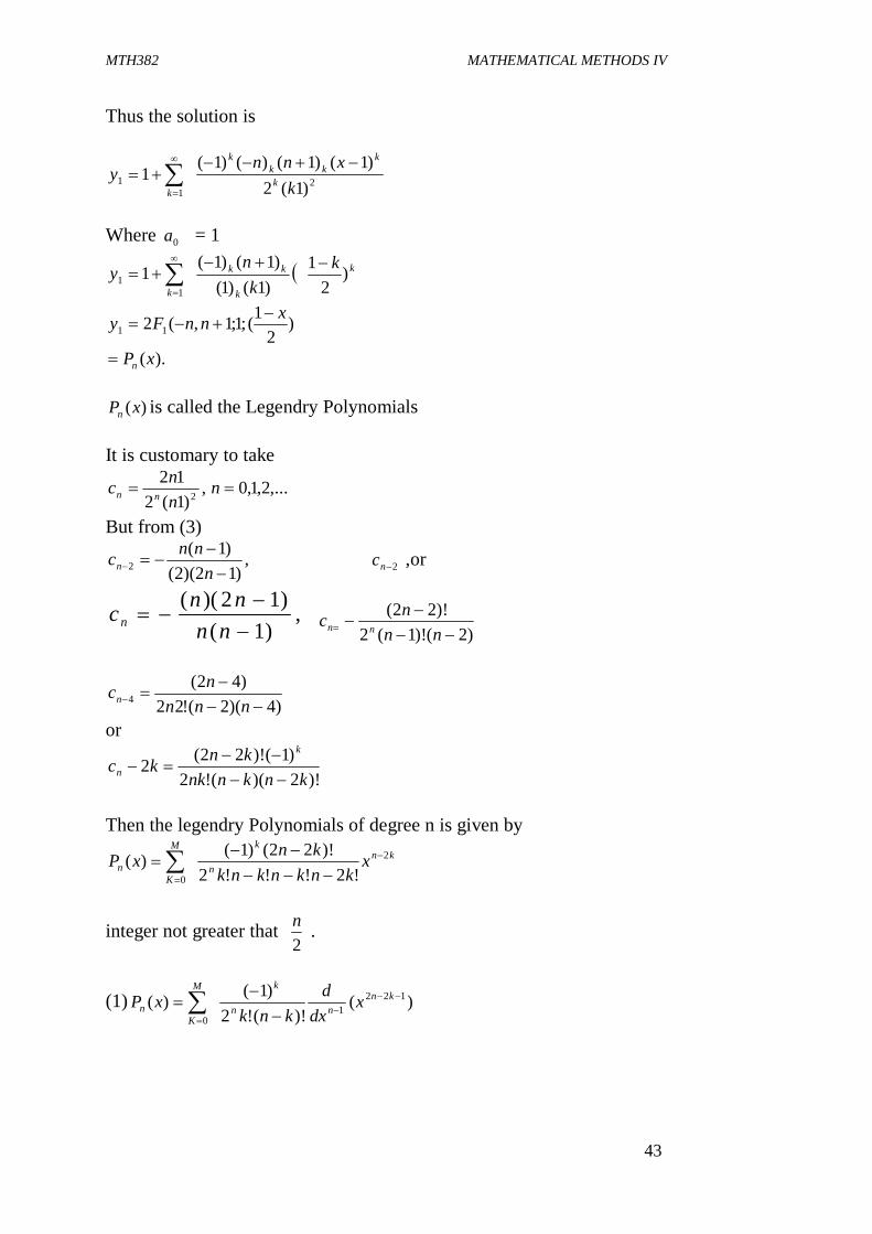
Thus the solution is
21
1 )1(2)1()1()()1(
1k
xnny k
kkk
k
k
Where 0a = 1
k
k
kk
k
kk
ny )2
1)1()1(
)1()1(1
11
)2
1(;1;1,(2 11xnnFy
).(xPn
)(xPn is called the Legendry Polynomials It is customary to take
,)1(2
122n
nc nn ,...2,1,0n
But from (3)
,)12)(2(
)1(2
n
nncn 2nc ,or
,)1(
)12)((
nn
nncn )2()!1(2
)!22(
nn
nc nn
)4)(2(!22)42(
4
nnnncn
or
)!2)((!2)1()!22(2
knknnkknkc
k
n
Then the legendry Polynomials of degree n is given by
knn
kM
Kn x
knknknkknxP 2
0 !2!!!2)!22()1()(
integer not greater that 2n .
(1) )()!(!2
)1()( 1221
0
knnn
kM
Kn x
dxd
knkxP
MTH382 MATHEMATICAL METHODS IV
44
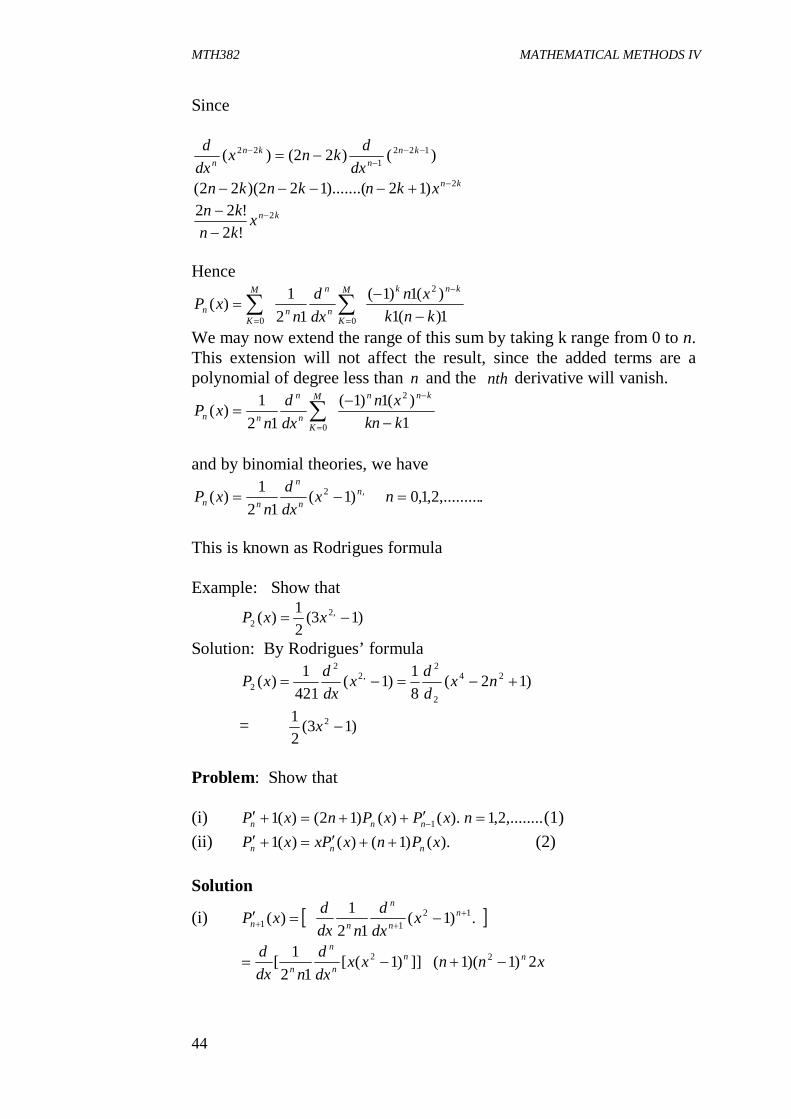
Since
)()22()( 1221
22
knn
knn dx
dknxdxd
knxknknkn 2)12).......(122)(22( knx
knkn 2
!2!22
Hence
1)(1)(1)1(
121)(
2
00 knkxn
dxd
nxP
knkM
Kn
n
n
M
Kn
We may now extend the range of this sum by taking k range from 0 to n. This extension will not affect the result, since the added terms are a polynomial of degree less than n and the nth derivative will vanish.
1)(1)1(
121)(
2
0 kknxn
dxd
nxP
knnM
Kn
n
nn
and by binomial theories, we have
,2 )1(12
1)( nn
n
nn xdxd
nxP .,.........2,1,0n
This is known as Rodrigues formula Example: Show that
)13(21)( ,2
2 xxP
Solution: By Rodrigues’ formula
)12(81)1(
4211)( 24
2
2,2
2
2 nxddx
dxdxP
= )13(21 2 x
Problem: Show that (i) ).()()12()(1 1 xPxPnxP nnn ,........2,1n (1) (ii) ).()1()()(1 xPnxPxxP nnn (2) Solution
(i) .)1(12
1)( 1211
n
n
n
nn xdxd
ndxdxP
]])1([12
1[ 2 nn
n
n xxdxd
ndxd
xnn n 2)1)(1( 2
MTH382 MATHEMATICAL METHODS IV
45
])1([21 2
1
1
1n
n
n
nn xxdxd
])([21 2
11n
n
n
nn xxdxd
])1(2)1)(12[(21 122
1 nn
n
n
nn xnxndxd
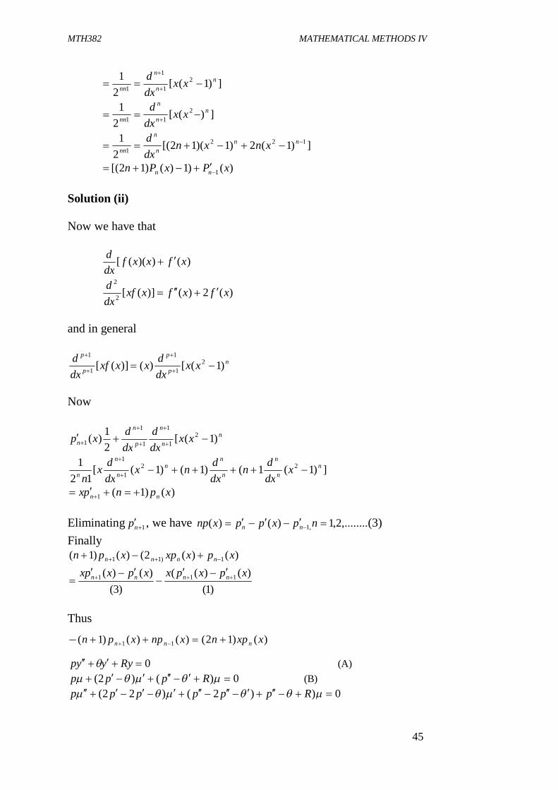
)()1)()12[( 1 xPxPn nn Solution (ii) Now we have that
)())(([ xfxxfdxd
)(2)()]([2
2
xfxfxxfdxd
and in general
np
p
p
p
xxdxdxxxf
dxd )1([)()]([ 2
1
1
1
1
Now
nn
n
p
n
n xxdxd
dxdxp )1([
21)( 2
1
1
1
1
1
])1(1()1()1([12
1 221
1n
n
n
n
nn
n
n
n xdxdn
dxdnx
dxdx
n
)()1(1 xpnpx nn Eliminating 1np , we have ,........2,1)()( ,1 npxppxnp nn (3) Finally
)()(2()()1( 1)11 xpxxpxpn nnnn
)1()()((
)3()()( 111 xpxpxxpxpx nnnn
Thus
0 Ryyyp (A) 0)()2( Rppp (B)
0))2()22( Rpppppp
)()12()()()1( 11 xxpnxnpxpn nnn

MTH382 MATHEMATICAL METHODS IV
46
4.0 CONCLUSION You have learnt about legendry polynomial and legendry functions in this unit. Read this unit properly before going to the next unit. 5.0 SUMMARY You will recall that the legendry polynomial is defined as:
knn
kM
Kn x
knknknkknxP 2
0 !2!!!2)!22()1()(
This polynomial has Orthogonality property which we have mentioned in this unit. 6.0 TUTOR-MARKED ASSIGNMENT 1. Show that the substitution xt 1 transform Legendre’s equation
to the form:
0)1()1(2)2( 2
2
yppdtdyt
dtydtt
2. Problem: Show that a. ).()()12()( 11 xPxPnxP nnn
,........2,1n b. ).()1()()(1 xPnxPxxP nnn
7.0 REFERENCES/FURTHER READING Earl, A. Coddington (nd). An Introduction to Ordinary Differential
Equations. India: Prentice-Hall. Einar, Hille (nd). Lectures on Ordinary Differential Equations. London:
Addison-Wesley Publishing Company. Francis, B. Hildebrand (nd). Advanced Calculus for Applications. New
Jersey: Prentice-Hall.
MTH382 MATHEMATICAL METHODS IV
47
UNIT 2 SOME EXAMPLES OF PARTIAL DIFFERENTIAL EQUATIONS
CONTENTS 1.0 Introduction 2.0 Objectives 3.0 Main Content 3.1 Some Examples of Partial Differential Equations 4.0 Conclusion 5.0 Summary 6.0 Tutor-Marked Assignment 7.0 References/Further Reading 1.0 INTRODUCTION A partial differential equation is an equation that contains one or more partial derivatives. Such equations occur frequently in application of mathematics. We shall only discuss certain partial differential equations which are used frequently in applied mathematics. In fact, we are going to discuss a kind of boundary value problems which enters modern applied mathematics at every turn. 2.0 OBJECTIVES At the end of this unit, you should be able to: recognise partial differential equations by type and character explain the methods of solving partial differential equations apply the knowledge in some other related field. 3.0 MAIN CONTENT 3.1 Some Examples of Partial Differential Equations in
Applied Mathematics Many linear problems in applied mathematics involve the solution of an equation obtained by specialising the form.
dtd
dtdf
2
22 (1)
Where f is a specified function of position and and are certain specified physical constant. Here, 2 is the Laplacian operator in one, two or dimension under consideration and is of the form.
MTH382 MATHEMATICAL METHODS IV
48
2
2
2
2
2
22
dzd
dyd
dxd
(2)
In rectangular co-coordinator of three space, the unknown function is the function of the position co-ordinates (x, y, z) and the tine t. (i) Laplace Equation
02 (3) It is satisfied by the velocity potential in an ideal incompressible fluid without vertical or continuously distributed sources; and by gravitational potential in free space; electrostatic potential in the steady flow of electric currents in solid conductors, and by the steady-state temperature distribution in solids. (ii) Poisson’s Equation
02 f (4) is satisfied, for example, by the velocity potential of an incompressible, irrotational, ideal fluid with continuously distributed sources or by steady temperature distribution due to distributed heat sources, and by a ‘sheds function’ involved in the elastic torsion of prismatic bars, with a suitably prescribed function .f (iii) Wave Equation
2
22 1
tc
(5)
This arises in the study of propagation of waves with velocity c, independent of the wave length. In particular, it is satisfied by the components of the electric or magnetic vector in electromagnetic theory, by suitably chosen component of displacement, in the theory of elastic vibrations, and by the velocity potential in the theory of sound (acoustics) for a perfect gas. (iv) The Equation of Heat Conduction
t
22 1 (6)
MTH382 MATHEMATICAL METHODS IV
49
This is satisfied, for example, by the temperature at a point of a homogeneous body and by the concentration of a diffused substance in the theory of diffusion, with a suitably prescribed constant . (v) The Telegraphic Equation
ttx
2
2
(7)
This is one dimensional specialisation of (1), and is satisfied by the potential in a telegraph cable, where Lc and ,Rc if the Leakage is neglected (L is inductance, c capacity and R resistance per unit length). (vi) Differential equation of higher order, involving the operator ,2
are rather frequently encountered, in particular, the bi-Laplacian equation in two dimensions.
02 22
2224
uu
u
yyxx
(8)
is involved in many two dimensional problem of the theory of elasticity. The solution of a given problem must satisfy the proper differential equation, together with similarly prescribed boundary condition or initial conditions (2 f time is involved). The above equation can be changed to cylindrical co-ordinates
,zr related to x, y and z by the equations
zzrSinyrCosx ,,
0121
21
2
2
2
2
22
22
zrrrr
(9) In spherical co-ordinates ,,P related to zyx ,, by the equations
PCoszPSinyCosPSinx ,, . Laplace’ equation is
.0cot22
2
2
2
2
2
2
2
v
pCosv
pv
ev
pdpv (10)
In what now follows we shall solution methods of partial differential equations: Method of separation of variables Consider the equation
dtu
dxv
2
22 , 0,0 tlx (a)
MTH382 MATHEMATICAL METHODS IV
50
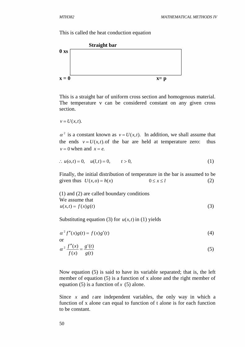
This is called the heat conduction equation Straight bar 0 xs x = 0 x= p This is a straight bar of uniform cross section and homogenous material. The temperature v can be considered constant on any given cross section.
).,( txUv
2 is a constant known as ).,( txUv In addition, we shall assume that the ends ).,( txUv of the bar are held at temperature zero: thus
0v when and .ex
,0),( tou ,0),( tlu ,0t (1) Finally, the initial distribution of temperature in the bar is assumed to be given thus )(),( xhoxU lx 0 (2) (1) and (2) are called boundary conditions We assume that
)()(),( tgxftxu (3) Substituting equation (3) for ),( txu in (1) yields
)()()()(2 tgxftgxf (4) or
)()('
)()(2
tgtg
xfxf
(5)
Now equation (5) is said to have its variable separated; that is, the left member of equation (5) is a function of x alone and the right member of equation (5) is a function of x (5) alone. Since x and t are independent variables, the only way in which a function of x alone can equal to function of t alone is for each function to be constant.
MTH382 MATHEMATICAL METHODS IV
51
bxfxf
)()( (6)
bxgxg
)()(2 (7)
In which b is arbitrary The partial differential equation (1) has now been replaced by two ordinary differential equations. This is the essence of the method of separation of variables. Boundary Conditions
0)()(),( tgoftoxv (8) by (1), if )(tg = 0 then tux, will be identically zero. It is not acceptable because it does not satisfy the equation (2). Thus it must satisfy the condition
0)( of (9) Similarly, the boundary condition at )(lx 0),( tlU requires
0)( lf (10) There are two possible values of the constant k i.e. 0k or .0k Values of the constant k : (i) 0k , then the general solution of equation (6) is 21)( ccxf (11) (11) Must satisfy the boundary value conditions (9) and (10). In order
to satisfy (9) 0)( 221 cccof (12) It is also satisfies the equation (10) 0)( 11 clclf Since .ol 01 c (13) Hence, )(xf is identically zero, and therefore 0,( txU is also identical zero
MTH382 MATHEMATICAL METHODS IV
52
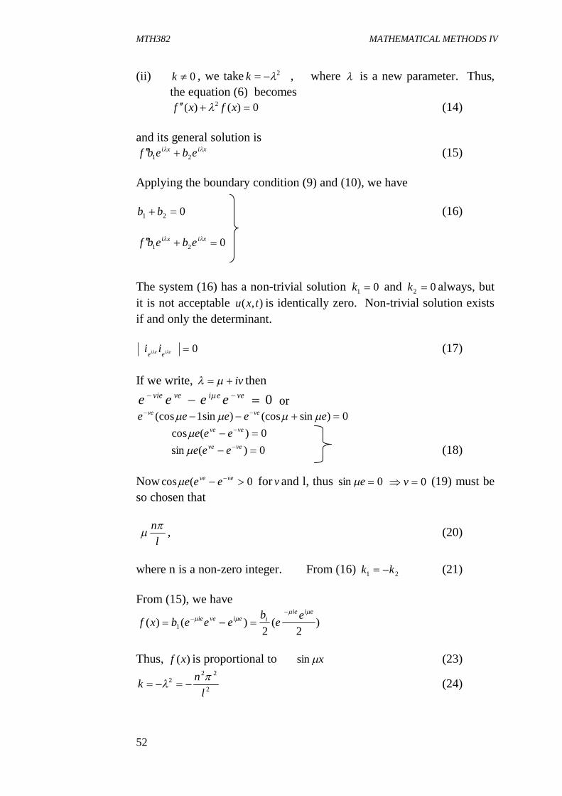
(ii) 0k , we take 2k , where is a new parameter. Thus, the equation (6) becomes
0)()( 2 xfxf (14) and its general solution is
xixi ebebf 21 (15)
Applying the boundary condition (9) and (10), we have
021 bb (16)
021 xixi ebebf The system (16) has a non-trivial solution 01 k and 02 k always, but it is not acceptable ),( txu is identically zero. Non-trivial solution exists if and only the determinant.
0eiei ee ii (17) If we write, iv then
0 veeivevie eeee or 0)sin(cos)sin1(cos eeeee veve
0)(cos veve eee 0)(sin veve eee (18) Now 0(cos veve eee for v and l, thus 0sin e 0 v (19) must be so chosen that
l
n , (20)
where n is a non-zero integer. From (16) 21 kk (21) From (15), we have
)2
(2
)()( 1
eiieieiveie eebeeebxf
Thus, )(xf is proportional to xsin (23)
2
222
lnk
(24)
MTH382 MATHEMATICAL METHODS IV
53
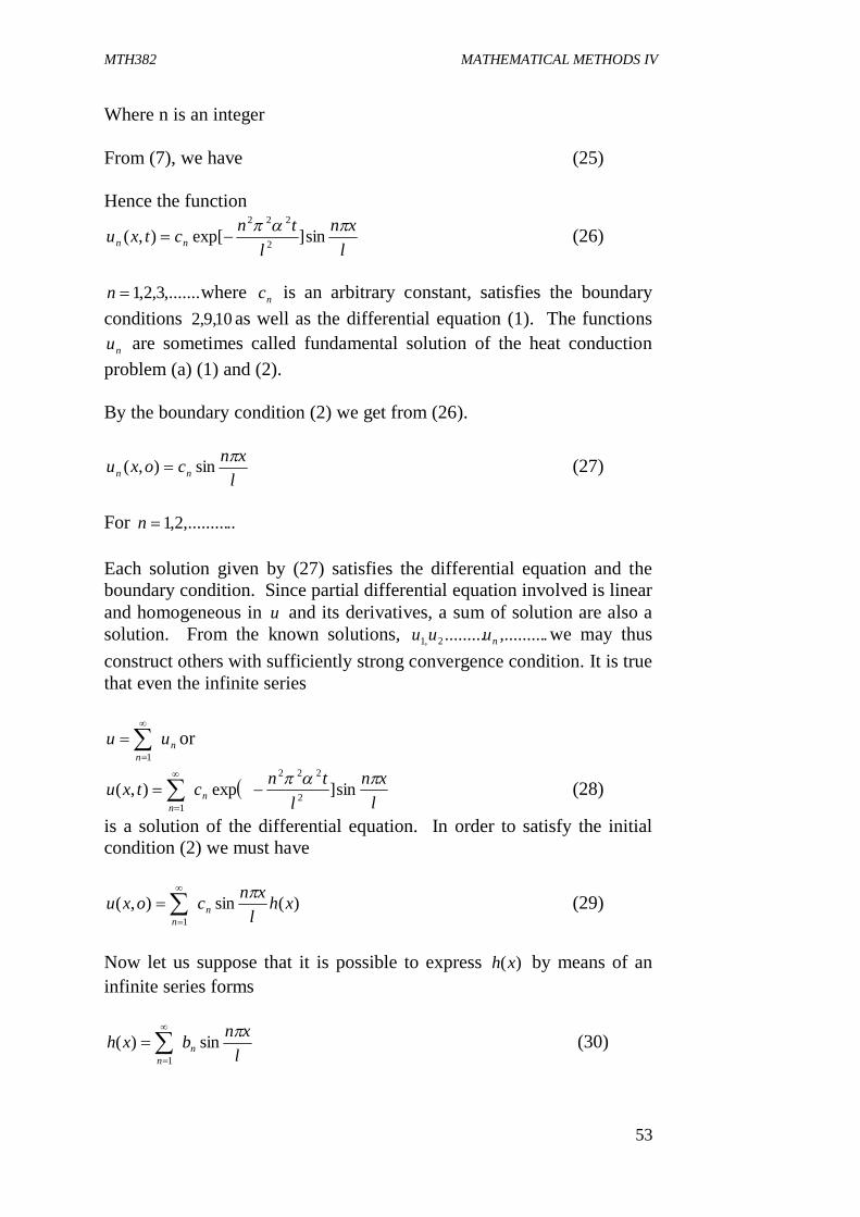
Where n is an integer From (7), we have (25) Hence the function
lxn
ltnctxu nn
sin]exp[),( 2
222
(26)
,.......3,2,1n where nc is an arbitrary constant, satisfies the boundary
conditions 10,9,2 as well as the differential equation (1). The functions nu are sometimes called fundamental solution of the heat conduction
problem (a) (1) and (2). By the boundary condition (2) we get from (26).
lxncoxu nnsin),( (27)
For ..,.........2,1n Each solution given by (27) satisfies the differential equation and the boundary condition. Since partial differential equation involved is linear and homogeneous in u and its derivatives, a sum of solution are also a solution. From the known solutions, .,..................2,1 nuuu we may thus construct others with sufficiently strong convergence condition. It is true that even the infinite series
nn
uu
1
or
lxn
ltnctxu n
n
sin]exp),( 2
222
1
(28)
is a solution of the differential equation. In order to satisfy the initial condition (2) we must have
)(sin),(1
xhlxncoxu n
n
(29)
Now let us suppose that it is possible to express )(xh by means of an infinite series forms
lxnbxh n
n
sin)(1
(30)
MTH382 MATHEMATICAL METHODS IV
54
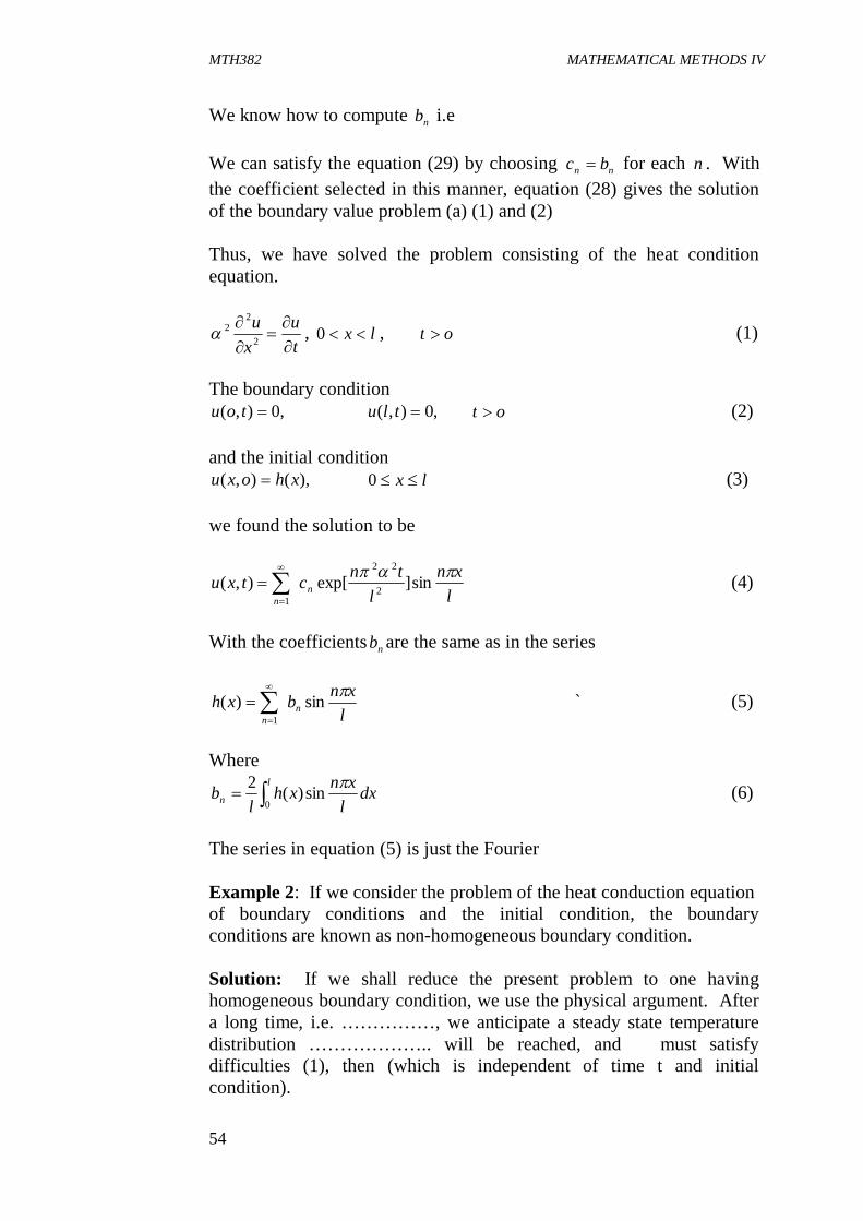
We know how to compute nb i.e We can satisfy the equation (29) by choosing nn bc for each n . With the coefficient selected in this manner, equation (28) gives the solution of the boundary value problem (a) (1) and (2) Thus, we have solved the problem consisting of the heat condition equation.
tu
xu
2
22 , lx 0 , ot (1)
The boundary condition
,0),( tou ,0),( tlu ot (2) and the initial condition
),(),( xhoxu lx 0 (3) we found the solution to be
lxn
ltnctxu n
n
sin]exp[),( 2
22
1
(4)
With the coefficients nb are the same as in the series
lxnbxh n
n
sin)(1
` (5)
Where
dxlxnxh
lb
l
n
0
sin)(2 (6)
The series in equation (5) is just the Fourier Example 2: If we consider the problem of the heat conduction equation of boundary conditions and the initial condition, the boundary conditions are known as non-homogeneous boundary condition. Solution: If we shall reduce the present problem to one having homogeneous boundary condition, we use the physical argument. After a long time, i.e. ……………, we anticipate a steady state temperature distribution ……………….. will be reached, and must satisfy difficulties (1), then (which is independent of time t and initial condition).

MTH382 MATHEMATICAL METHODS IV
55
…………. (4) and it satisfied the boundary condition …………. (5) Which apply even as …………….. The solution (4) with condition (5) ………….. (6) Hence the steady state temperature is a linear function of x. We shall express ),( txU as the sum of the steady state temperature and another distribution w(x, t). ),()(),( txxUtxU (7) (7) satisfies (1), we have twuxxwu )()(2 (8) It follows that txx WW 2 (9) Now boundary condition
0)(),(),( 11 TToutoutow (10)
0)(),(),( 22 TTlutlutlw (11) The initial condition
)()()(),((),( xuxfxuoxuoxw (12) Where u(x) is given by (6) The problem now becomes precisely the previous one and we have the solution
lxnSin
ltnbtxW n
n
222
1exp),(
(13)
Where
dxlxnSinxW
lb
l
n)0,(2
0 (14)
Where
lxnSin
ltnbT
lxTTtxU n
n
222
1112 exp)(),(
(15)

MTH382 MATHEMATICAL METHODS IV
56
Where
dxlxnSinT
lxTTxf
lb
l
n
1120)()(2
(16) Example 3: Now we consider the problem of the heat conduction equation with the boundary condition
xxx UU 2 (1)
0),0( tVx , 0),( tlVx , 0t (2) and the initial condition
)()0,( xfxv (3) Solution: We solve the equation by the method of separation of variables. [when the ends of the bar are insulated so that there is no passage of heat through them].
)()(),( tgxhtxV (4) (4) satisfies (1), we have
)()('1
)()('
2 tgtg
xhxh (5)
We assume that is real, we consider three cases = 0 and –ve. (i) If = 0 then equation (5) given
21),( KxKtxV (6) Applying boundary condition (2), we get
.01 K Hence corresponding 0)(' xh
21)( CCxh BCtgtg )(0)( (7)
Solution is (ii) If = 2 where is real and +ve
0)()( xhxh (8)
0)()( 2 xhtg (9) From (8) and (9), we have
).(),( 2122 xCoshkxSinhktxU
t
ex (10)
MTH382 MATHEMATICAL METHODS IV
57
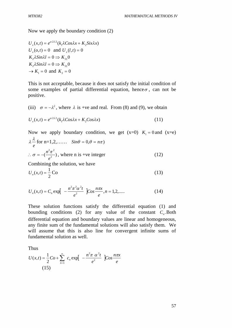
Now we apply the boundary condition (2)
)(),( 2122 xSixKxCosketxU x
0),( toU x and 0),( tlU x 00 122 KlSinK 00 122 KlSinK
01 K and 02 K This is not acceptable, because it does not satisfy the initial condition of some examples of partial differential equation, hence , can not be positive. (iii) 2 , where is +ve and real. From (8) and (9), we obtain
)(),( 2122 xCosKxCosketxU x (11)
Now we apply boundary condition, we get (x=0) 01 K and (x=e)
e
for n=1,2,…… ),0 nSin
)( 2
22
en
, where n is +ve integer (12)
Combining the solution, we have
21),( txUo Co (13)
,.....2,1,exp),( 2
222
ne
xnCose
tnCtxU nn (14)
These solution functions satisfy the differential equation (1) and bounding conditions (2) for any value of the constant .nC Both differential equation and boundary values are linear and homogeneous, any finite sum of the fundamental solutions will also satisfy them. We will assume that this is also line for convergent infinite sums of fundamental solution as well. Thus
e
xnCose
tncCotxU nn
2
22
1exp
21),(
(15)
MTH382 MATHEMATICAL METHODS IV
58
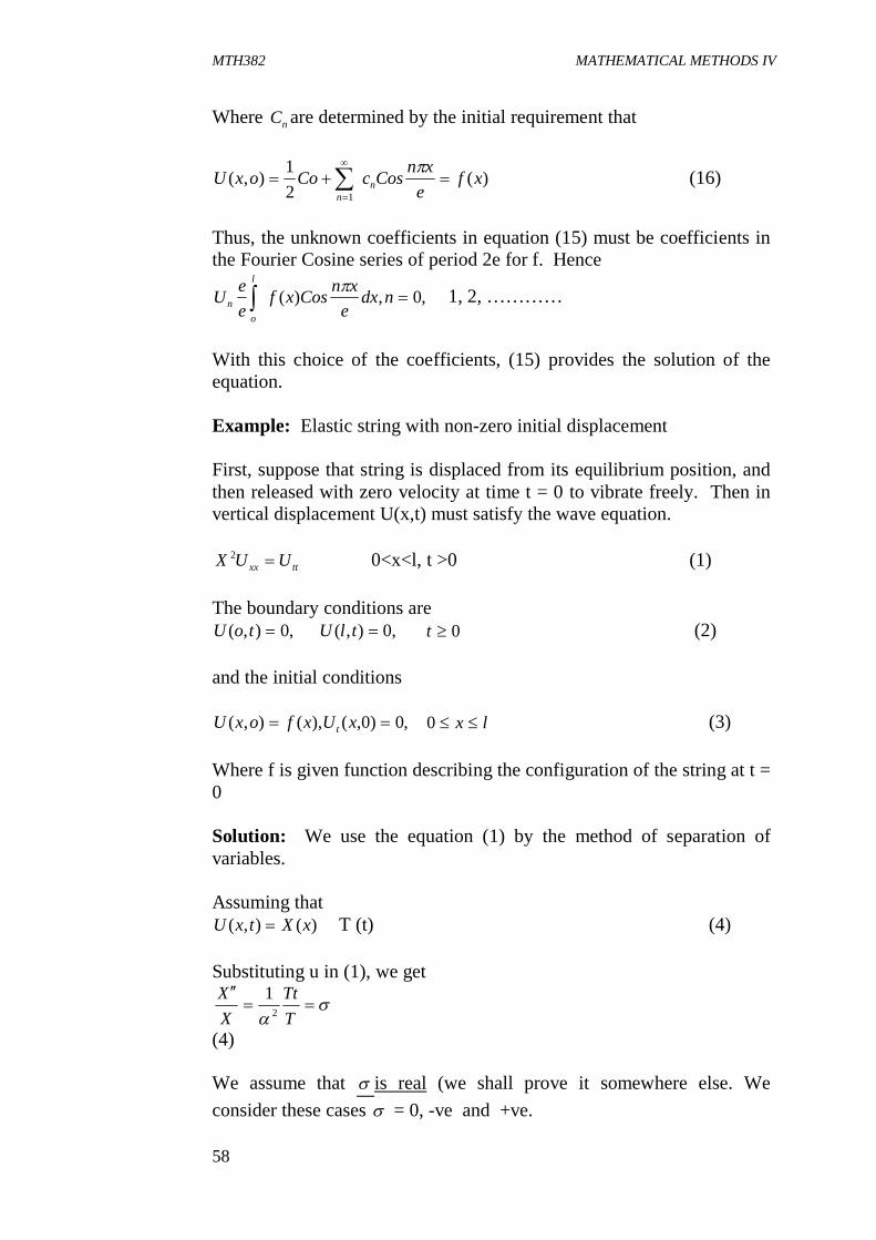
Where nC are determined by the initial requirement that
)(21
),(1
xfexnCoscCooxU n
n
(16)
Thus, the unknown coefficients in equation (15) must be coefficients in the Fourier Cosine series of period 2e for f. Hence
,0,)( ndxe
xnCosxfeeU
l
on
1, 2, …………
With this choice of the coefficients, (15) provides the solution of the equation. Example: Elastic string with non-zero initial displacement First, suppose that string is displaced from its equilibrium position, and then released with zero velocity at time t = 0 to vibrate freely. Then in vertical displacement U(x,t) must satisfy the wave equation.
ttxx UUX 2 0<x<l, t >0 (1) The boundary conditions are
,0),( toU ,0),( tlU 0t (2) and the initial conditions
,0)0,(),(),( xUxfoxU t lx 0 (3) Where f is given function describing the configuration of the string at t = 0 Solution: We use the equation (1) by the method of separation of variables. Assuming that
)(),( xXtxU T (t) (4) Substituting u in (1), we get
TTt
XX
2
1
(4) We assume that is real (we shall prove it somewhere else. We consider these cases = 0, -ve and +ve.
MTH382 MATHEMATICAL METHODS IV
59
(i) = 0, then ,0X and 21)( KxKxX (5) (ii) If ,0 then 02 xX and xCoshKxSinhKxX 21)( (6) Where Consider the solution given by (5)
)()(),( 21 tTKxKtxU By boundary conditions 0),( toU
,0)()0(),( 2 tTKtoU )(tT can not be zero, because U(x,t) will be identically zero. Thus, .02 K Next consider the second boundary condition 0),( tlU then 00)()(),( 11 KtTlKtlU Thus X(x) = 0, it is not acceptable. (iii) Similarly, we can show that for (6) under boundary condition
.0 21 KK Thus, 0 and ve real number are not acceptable. We now consider the last cast (ii) 0 x (7) 0 XX (8) 022 TT xCosKSinKxX 21)( (9) tCosKtSinKtT u 2)( (10) Thus
))((),( 431 tCosKtSinKtCosKxSinKtxU (11) Satisfies (1) for all values of 4321 ,,, KKKK and for and .0 Now we impose the boundary conditions
,0),( toU Thus
0)(),( 2432 KtCosKtSinKKtoU (12)
MTH382 MATHEMATICAL METHODS IV
60
Secondly, boundary condition ,0),( tlU
0))((),( 31 tCosKtSinKlSinKtlU u (13) If ,01 K then U (x,t) is zero identically, thus for non-trivial solution.
........2,1,0 nl
nlSin (14)
Hence the functions which satisfy the equation (1) and boundary condition (2) are of the form.
)(),(l
tnCosKl
tnSinClxnSintxU nnn
(15)
Where n=1,2,…….. nC and nK are arbitrary constants. Now we apply the principle of super position of solution and assume that
),(),(1
trUtxU nn
n
)(1 l
tnCosKl
tnSinClxnSin nn
n
(16) Further, we assume that (16) can be differentiated term by term with respect to t
0),( oxU t yields
0),(1
lxnSin
lanCoxU n
nn
(17)
0 nC for all values of n The other condition )(),( xfoxU Given
)(),(1
xflanSinKoxU n
nn
(18) Consequently, nK must be line coefficients in the Fourier Series of period 2 l for f and are given by
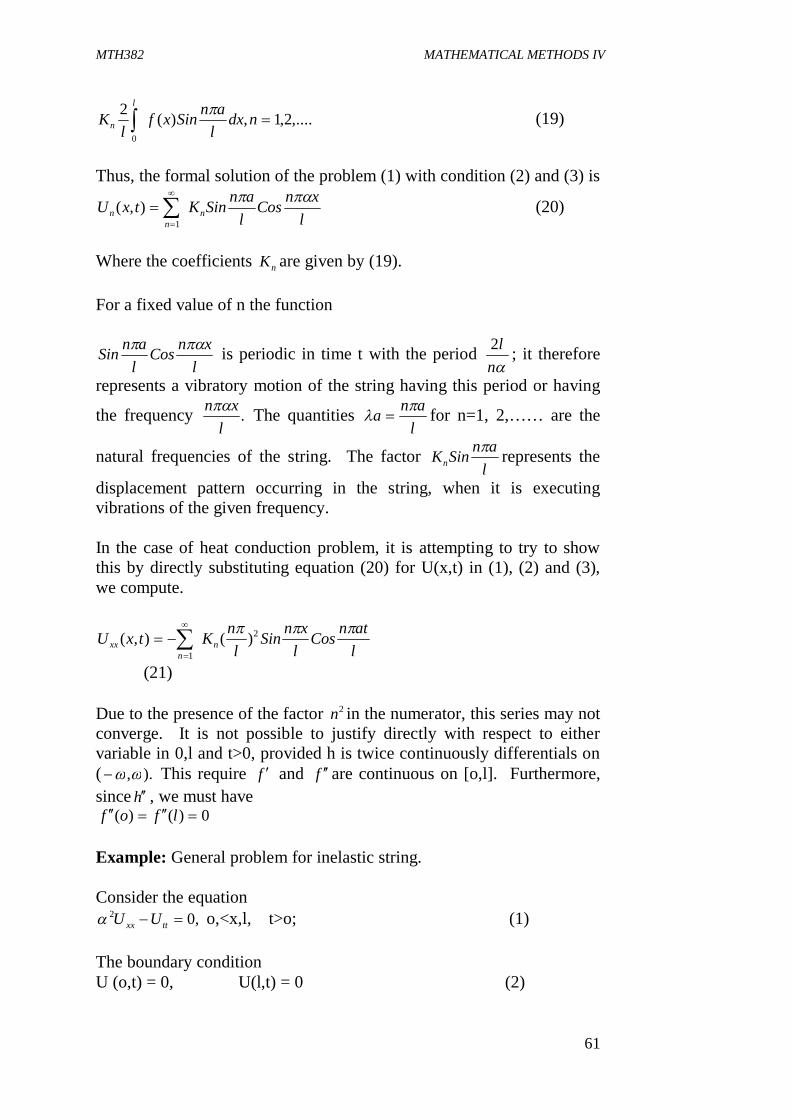
MTH382 MATHEMATICAL METHODS IV
61
,....2,1,)(2
0
ndxlanSinxf
lK
l
n (19)
Thus, the formal solution of the problem (1) with condition (2) and (3) is
lxnCos
lanSinKtxU n
nn
1
),( (20)
Where the coefficients nK are given by (19). For a fixed value of n the function
lxnCos
lanSin is periodic in time t with the period
nl2 ; it therefore
represents a vibratory motion of the string having this period or having
the frequency .l
xn The quantities lana
for n=1, 2,…… are the
natural frequencies of the string. The factor lanSinKn represents the
displacement pattern occurring in the string, when it is executing vibrations of the given frequency. In the case of heat conduction problem, it is attempting to try to show this by directly substituting equation (20) for U(x,t) in (1), (2) and (3), we compute.
latnCos
lxnSin
lnKtxU n
nxx
2
1)(),(
(21) Due to the presence of the factor 2n in the numerator, this series may not converge. It is not possible to justify directly with respect to either variable in 0,l and t>0, provided h is twice continuously differentials on ( )., This require f and f are continuous on [o,l]. Furthermore, since h , we must have
0)()( lfof Example: General problem for inelastic string. Consider the equation
,02 ttxx UU o,<x,l, t>o; (1) The boundary condition U (o,t) = 0, U(l,t) = 0 (2)
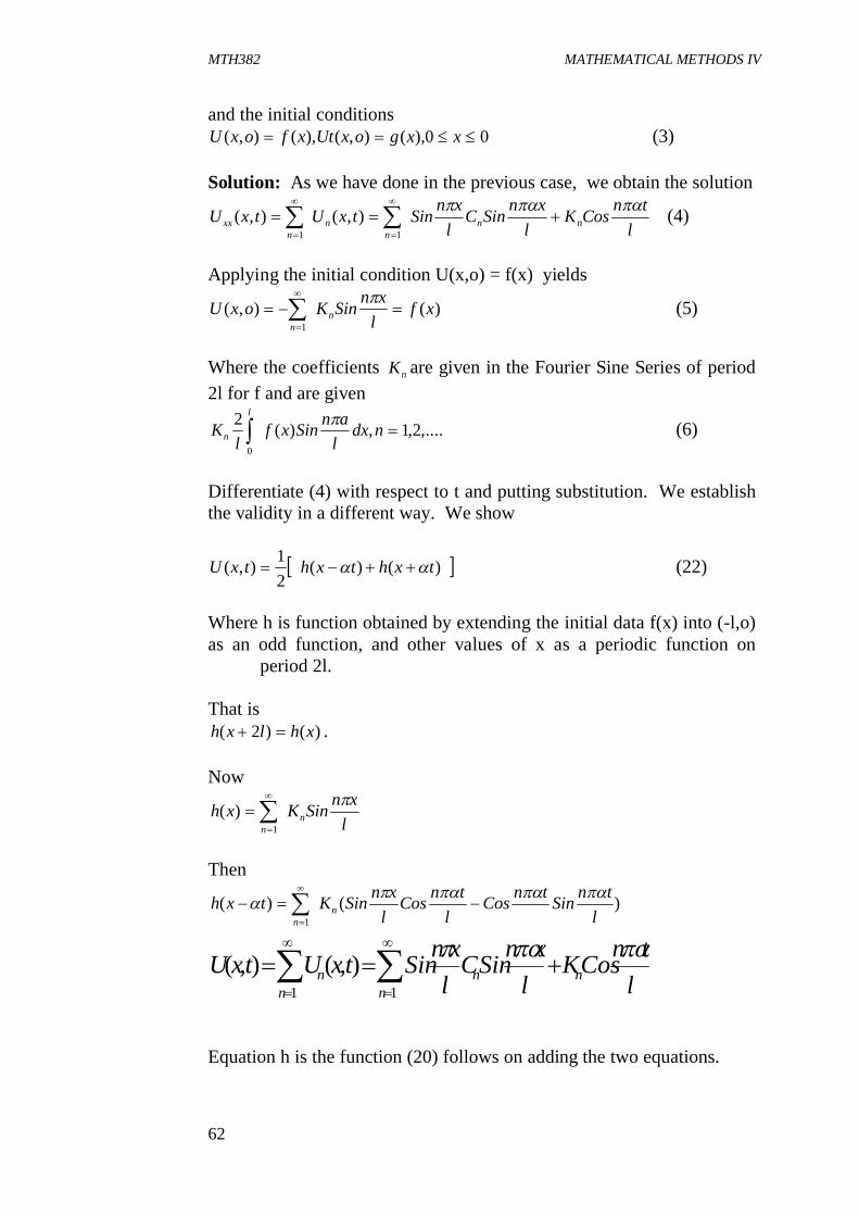
MTH382 MATHEMATICAL METHODS IV
62
and the initial conditions 00),(),(),(),( xxgoxUtxfoxU (3)
Solution: As we have done in the previous case, we obtain the solution
ltnCosK
lxnSinC
lxnSintxUtxU nn
nn
nxx
11),(),( (4)
Applying the initial condition U(x,o) = f(x) yields
)(),(1
xflxnSinKoxU n
n
(5)
Where the coefficients nK are given in the Fourier Sine Series of period 2l for f and are given
,....2,1,)(2
0
ndxlanSinxf
lK
l
n (6)
Differentiate (4) with respect to t and putting substitution. We establish the validity in a different way. We show
)()(21),( txhtxhtxU (22)
Where h is function obtained by extending the initial data f(x) into (-l,o) as an odd function, and other values of x as a periodic function on period 2l. That is
)()2( xhlxh . Now
lxnSinKxh n
n
1
)(
Then
)()(1 l
tnSintnCosl
tnCoslxnSinKtxh n
n
ltnCosK
lxnSinC
lxnSintxUtxU nn
nn
n
11
),(),(
Equation h is the function (20) follows on adding the two equations.
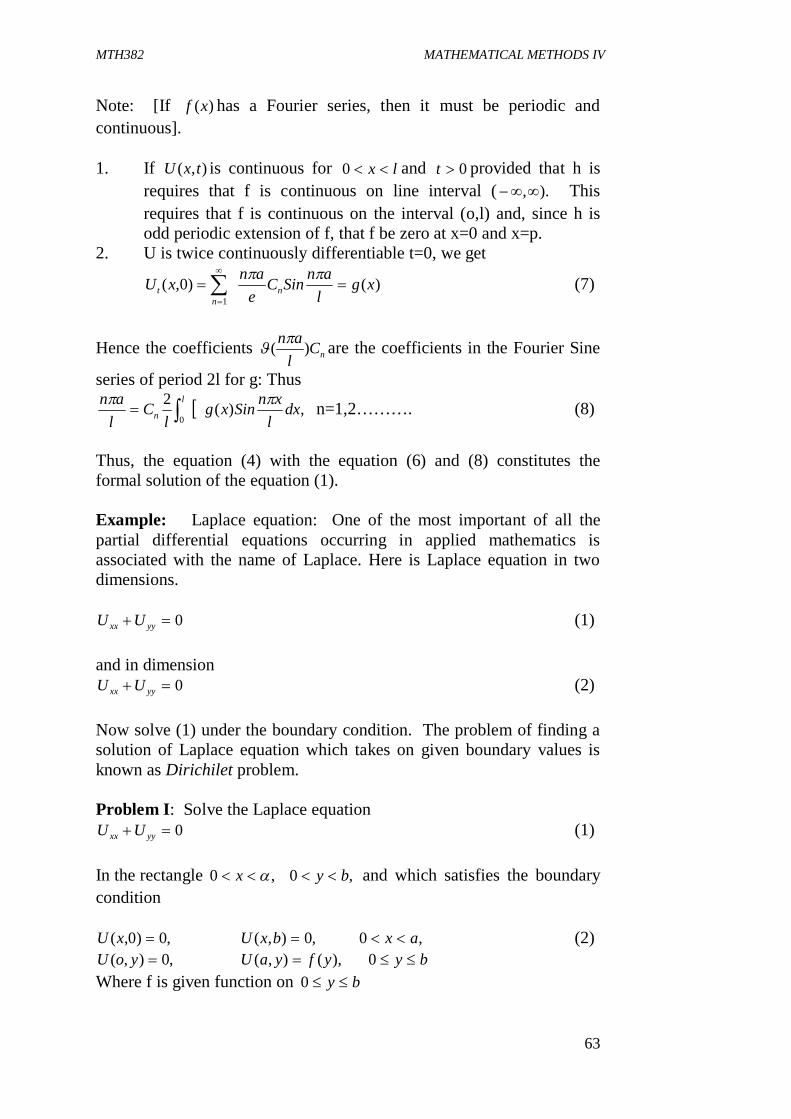
MTH382 MATHEMATICAL METHODS IV
63
Note: [If )(xf has a Fourier series, then it must be periodic and continuous]. 1. If ),( txU is continuous for lx 0 and 0t provided that h is
requires that f is continuous on line interval ( )., This requires that f is continuous on the interval (o,l) and, since h is odd periodic extension of f, that f be zero at x=0 and x=p.
2. U is twice continuously differentiable t=0, we get
)()0,(1
xglanSinC
eanxU n
nt
(7)
Hence the coefficients nClan )(
are the coefficients in the Fourier Sine
series of period 2l for g: Thus
,)(20
dxlxnSinxg
lC
lan l
n
n=1,2………. (8)
Thus, the equation (4) with the equation (6) and (8) constitutes the formal solution of the equation (1). Example: Laplace equation: One of the most important of all the partial differential equations occurring in applied mathematics is associated with the name of Laplace. Here is Laplace equation in two dimensions.
0 yyxx UU (1) and in dimension
0 yyxx UU (2) Now solve (1) under the boundary condition. The problem of finding a solution of Laplace equation which takes on given boundary values is known as Dirichilet problem. Problem I: Solve the Laplace equation
0 yyxx UU (1) In the rectangle ,0 x ,0 by and which satisfies the boundary condition
,0)0,( xU ,0),( bxU ,0 ax (2) ,0),( yoU ),(),( yfyaU by 0
Where f is given function on by 0
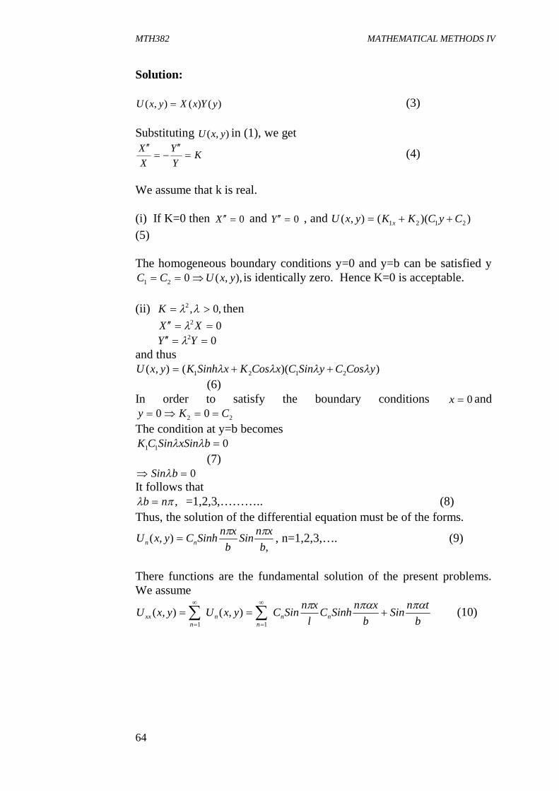
MTH382 MATHEMATICAL METHODS IV
64
Solution:
)()(),( yYxXyxU (3) Substituting ),( yxU in (1), we get
KYY
XX
(4)
We assume that k is real. (i) If K=0 then 0X and 0Y , and ))((),( 2121 CyCKKyxU x (5) The homogeneous boundary conditions y=0 and y=b can be satisfied y
),,(021 yxUCC is identically zero. Hence K=0 is acceptable. (ii) ,0,2 K then 02 XX 02 YY and thus
))((),( 2121 yCosCySinCxCosKxSinhKyxU (6) In order to satisfy the boundary conditions 0x and
22 00 CKy The condition at y=b becomes
011 bxSinSinCK (7)
0 bSin It follows that
, nb =1,2,3,……….. (8) Thus, the solution of the differential equation must be of the forms.
,),(
bxnSin
bxnSinhCyxU nn
, n=1,2,3,…. (9)
There functions are the fundamental solution of the present problems. We assume
btnSin
bxnSinhC
lxnSinCyxUyxU nn
nn
nxx
11),(),( (10)
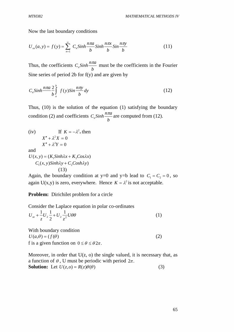
MTH382 MATHEMATICAL METHODS IV
65
Now the last boundary conditions
bynSin
bxnSinh
banSinhCyfyaU n
nxx
1
)(),( (11)
Thus, the coefficients b
anSinhCn must be the coefficients in the Fourier
Sine series of period 2b for f(y) and are given by
dyb
ynSinyfb
anSinhCb
on
)(2 (12)
Thus, (10) is the solution of the equation (1) satisfying the boundary
condition (2) and coefficients b
anSinhCn are computed from (12).
(iv) If nK 2 then 02 XX 02 YX and
)(),( 21 xCosKxSinhKyxU )),( 21 yCoshCySinhyxC (13) Again, the boundary condition at y=0 and y=b lead to 021 CC , so again U(x,y) is zero, everywhere. Hence 2K is not acceptable. Problem: Dirichilet problem for a circle Consider the Laplace equation in polar co-ordinates
Uz
UUz
U zz 2221
211 (1)
With boundary condition
)((),( faU (2) f is a given function on .20 Moreover, in order that U(z, o) the single valued, it is necessary that, as a function of , U must be periodic with period .2 Solution: Let )()(),( zRozU (3)

MTH382 MATHEMATICAL METHODS IV
66
We substitute (3) in (1)
0121
2 Rr
Rr
Or
KRRz
RRr
2 (4)
Again, we assume that the separation constant must be real. (1) Suppose K=0 02 RrRr 0
2(),( 21 LogKKrU 21)( CC )(2(),( 2121 CCLogKKrU (5) Since equation is periodic in , thus .02 C Further 0r the term log r is unbounded. This behaviour is unacceptable. Thus, we impose the condition that U (z, o) remains finite at all points of the circle and hence we must take
02 K
),(0 orU Constant = 021 c say (6)
(ii) If 2K then 02 (7) eCC 21)( (8) The function ),( orU is periodic thus .021 CC This makes )0,(rU identically zero. This is not acceptable. (iii) Finally, ,0,2 K yields 022 RRrRr (9) And 02 (10)
rKrKrR 21)(
CosCSinC 21)( (11) In order that be periodic with period 2 , it is necessary that be a positive integer.
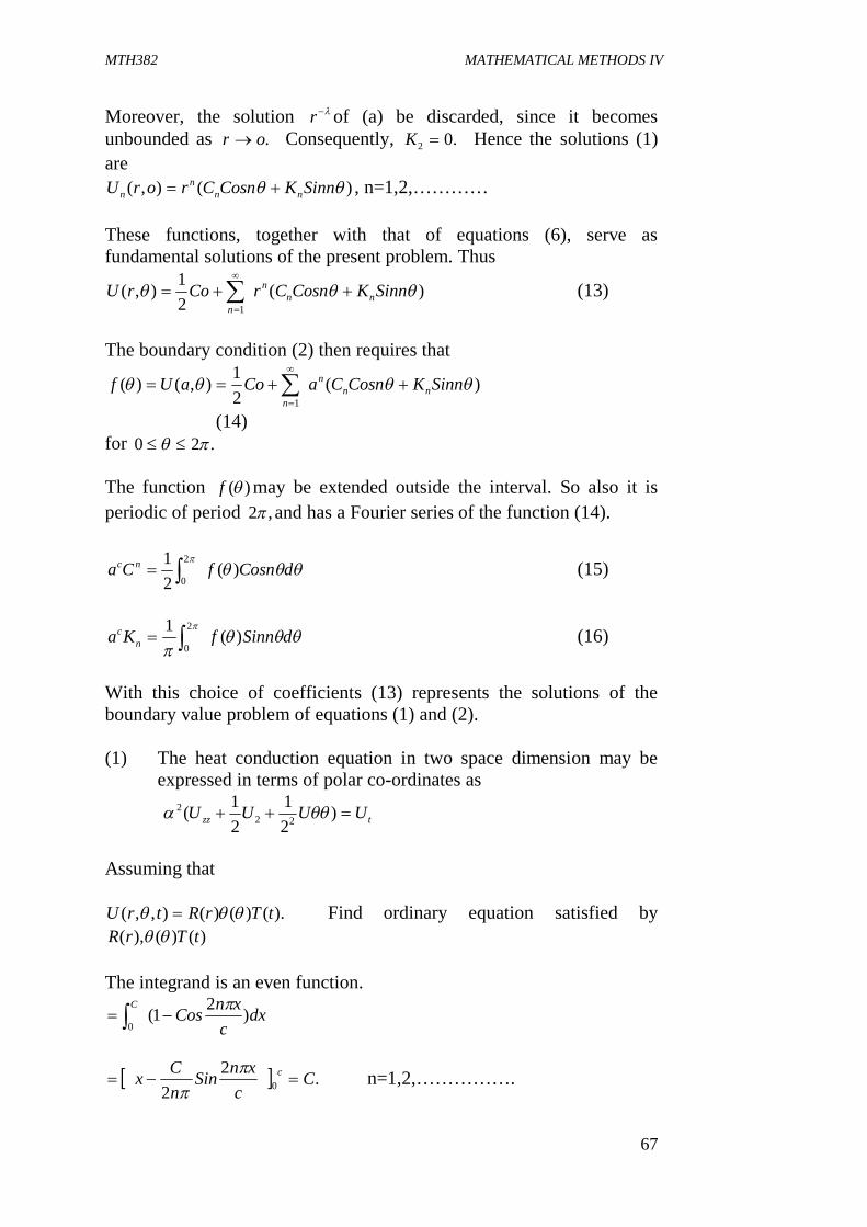
MTH382 MATHEMATICAL METHODS IV
67
Moreover, the solution r of (a) be discarded, since it becomes unbounded as .or Consequently, .02 K Hence the solutions (1) are
)(),( SinnKCosnCrorU nnn
n , n=1,2,………… These functions, together with that of equations (6), serve as fundamental solutions of the present problem. Thus
)(21
),(1
SinnKCosnCrCorU nnn
n
(13)
The boundary condition (2) then requires that
)(21
),()(1
SinnKCosnCaCoaUf nnn
n
(14) for .20 The function )(f may be extended outside the interval. So also it is periodic of period ,2 and has a Fourier series of the function (14).
dCosnfCa nc )(21 2
0 (15)
dSinnfKa n
c )(1 2
0 (16)
With this choice of coefficients (13) represents the solutions of the boundary value problem of equations (1) and (2). (1) The heat conduction equation in two space dimension may be
expressed in terms of polar co-ordinates as
tzz UUUU )21
21( 22
2
Assuming that
).()()(),,( tTrRtrU Find ordinary equation satisfied by )()(),( tTrR
The integrand is an even function.
dxc
xnCosC
)21(0
.22 0 C
cxnSin
nCx c
n=1,2,…………….
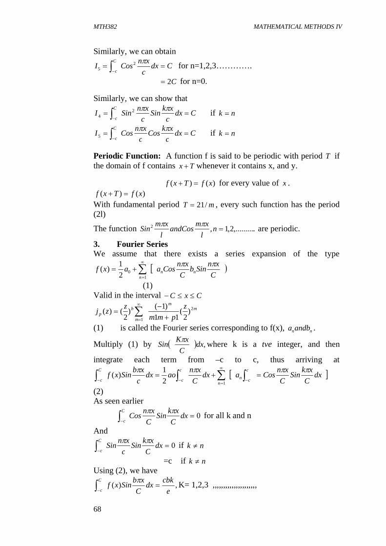
MTH382 MATHEMATICAL METHODS IV
68
Similarly, we can obtain
Cdxc
xnCosIC
c
25 for n=1,2,3………….
C2 for n=0. Similarly, we can show that
Cdxc
xkSinc
xnSinIC
c
24 if nk
Cdxc
xkCosc
xnCosIC
c
5 if nk
Periodic Function: A function f is said to be periodic with period T if the domain of f contains Tx whenever it contains x, and y. )()( xfTxf for every value of x .
)()( xfTxf With fundamental period mT /21 , every such function has the period (2l)
The function .,.........2,1,2 nl
xmandCosl
xmSin are periodic.
3. Fourier Series We assume that there exists a series expansion of the type
C
xnSinbC
xnCosaaxf nnn
1
021
)(
(1) Valid in the interval CxC
mm
m
bp
zpmm
zzj 2
1)
2(
11)1()
2()(
(1) is called the Fourier series corresponding to f(x), nnandba .
Multiply (1) by ,dxC
xKSin where k is a tve integer, and then
integrate each term from –c to c, thus arriving at
dxC
xkSinC
xnCosadxC
xnaodxcxbSinxf
c
cnn
c
c
C
c
121
)(
(2) As seen earlier
0 dxC
xkSinC
xnCosC
c
for all k and n
And
0 dxC
xkSinc
xnSinC
c
if nk
=c if nk Using (2), we have
,)(e
cbkdxC
xbSinxfC
c
K= 1,2,3 ,,,,,,,,,,,,,,,,,,,,,
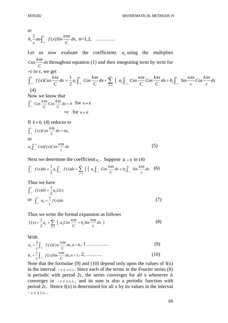
MTH382 MATHEMATICAL METHODS IV
69
or
,)(1 dxC
xnSinxfaoc
bc
cn
n=1,2, ………… Let us now evaluate the coefficients .na using the multiplies
dxC
xkCos throughout equation (1) and then integrating term by term for
–c to c, we get
dxcxkCos
cxnSinbdx
CxkCos
CxnCosadx
CxkCosadx
CxkCosxf
c
cncnn
c
co
C
c
12
1)(
(4) Now we know that
0 dxC
xkCosC
xnCosC
c
for kn
=c for kn If ,0k (4) reduces to
k
C
ceadx
CxkCosxf )(
or dx
cxnCosxCosfa
c
cn)(
(5)
Next we determine the coefficient na . Suppose 0K in (4)
dxc
xnSinbdxC
xnCosadxxfadxxfc
cncnn
c
co
C
c
1
)(21)( (6)
Thus we have
)2(21)( 0 cadxxf
C
c
or dxxfc
aC
c)(1
0 (7)
Thus we write the formal expansion as follows
dxc
xnSinbC
xnCosaaxf nnn
o
121)( (8)
With
0,)(1 ndx
CxnCosxf
ca
cn , 1 …………. (9)
1,)(1 ndx
CxnSinxf
cb
cn , 2, ………. (10)
Note that the formulae (9) and (10) depend only upon the values of f(x) in the interval .cxc Since each of the terms in the Fourier series (8) is periodic with period 2c, the series converges for all x whenever it converges in .cxc , and its sum is also a periodic function with period 2c. Hence f(x) is determined for all x by its values in the interval
.cxc .

MTH382 MATHEMATICAL METHODS IV
70
4.0 CONCLUSION You have been introduced to partial differential equation in this unit. The attempts here are just introductory. You are required to study this unit properly because you will refer to it in your subsequent courses in mathematics. 5.0 SUMMARY In this unit, various forms and types of partial differential equations were studied. These include (1) Wave equation (2) Laplace equation and (3) Heat equation. We also proposed various methods of solving these equations which include method of separation of variables and Fourier series applications. You are required to study this unit properly and attempt all the exercises at the end of the unit. 6.0 TUTOR-MARKED ASSIGNMENT 1. Show that the boundary-value problem
0)()0(,022
2
lyyykdx
yd cannot have a nontrivial solution for
real values of k 2. Determine those values of k for which the partial differential
equation
02
2
2
2
yT
xT possesses nontrivial solutions of the form
kyxfyxT sinh)(),( which vanish when lxwhenandx ,,,0 3. By considering the characteristic functions of the problem
,02)1( 2
22 y
dxdyx
dxydx
Show that 0)()(1
1 dxxPxP sr
7.0 REFERENCES/FURTHER READING Earl, A. Coddington (nd). An Introduction to Ordinary Differential
Equations. India: Prentice-Hall. Einar, Hille (nd). Lectures on Ordinary Differential Equations. London:
Addison-Wesley Publishing Company. Francis, B. Hildebrand (nd). Advanced Calculus for Applications. New
Jersey: Prentice-Hall.