Music Classification Using Kolmogorov Distance

Zehra Cataltepe, Abdullah Sonmez, Esref Adali

Istanbul Technical University

{zehra, adali}@cs.itu.edu.tr

Abstract. We evaluate the music composer classification using an approximation of the Kolmogorov distance be-

tween different music pieces. The distance approximation has recently been suggested by Vitanyi and his col-

leagues. They use a clustering method to evalute the distance metric. However the clustering is too slow for large

(>60) data sets. We suggest using the distance metric together with a k-nearest neighbor classifier. We measure the

performance of the distance metric based on the test classification accuracy of the classifier. A classification accu-

racy of 79% is achieved for a training data set of 57 midi files from three different classical composers. We find out

that the classification accuracy increases with training set size. The performance of the metric seems to also depend

on different pre-processing methods, hence domain knowledge and input representation could make a difference on

how the distance metric performs.

1 Introduction

Recently Vitanyi and his colleagues (Cilibrasi and Vitanyi, Cilibrasi et.al., Li et. al.) have suggested using an ap-

proximation to Kolmogorov distance between two musical pieces as a means to compute clusters of music. They first

process the MIDI representation (www.midi.org) of a music piece to turn it into a string from a finite alphabet. Then

they compute the distance between two music pieces using their Normalized Compression Distance (NCD). NCD

uses the compressed length of a string as an approximation to its Kolmogorov Complexity.

Although the Kolmogorov Complexity of a string is not computable, the compressed length approximation seems

to have given good results for musical genre and composer clustering in (Cilibrasi et.al.) and other data sets (Keogh

et.al.). (Cilibrasi et.al.) note that the clustering performance decreases as the data size increases. In this paper, we

investigate how the performance of the distance metric changes with data set size. In order to be able to quantify our

results better, instead of clustering, we use classification. We classify the composer of a new music piece based on a

set of training data from different composers. We use k-nearest neighbor (Bishop 57) as the classifier, since it only

requires the distance between feature vectors.

Like Vitanyi and colleagues, we also work on midi (see www.midi.org) files. Although there is loss of quality and

information from mp3 or wav to midi format and midi has its other limitations, this format takes a lot less space, is

widely accepted and allows for better comparison between music pieces played on different instruments. In this paper

we use different pre-processing methods of midi files and also report how pre-processing affects the performance of

the classifier. Polyphonic to monophonic conversions at different time two intervals and using the difference be-

tween notes at consecutive time intervals versus normalized notes with respect to the mathematical mode of the notes

in the piece are the four different pre-processing methods that we investigate.

In our data set, we use midi music pieces from 3 different classical composers (Bach, Chopin, Debussy). The midi

data we use was gathered from the internet.

2 Normalized Compression Distance (NCD)

For completeness of the paper, we repeat the derivation of the NCD (Cilibrasi et.al.) or K-metric (Ming and Sleep).

Please see the references for more information.

Given a string

!

x from a finite alphabet,

!

K(x) , the Kolmogorov Complexity of

!

x , is the length of the shortest

program that can output

!

x and halt (Cover 147).

!

K(x) can also be considered the length of the shortest compressed

binary version from which

!

x can be fully reproduced or the amount of information, number of bits in

!

x (Cilibrasi

et.al.).

!

K(x | y) can be considered the minimum number of bits to produce

!

x from string

!

y . We approximate

!

K(x) by the compressed length of

!

x . For

!

K(x | y)we use the approximation

!

K(x | y) " K(xy)#K(x) where

!

xy is the concatenation of strings

!

x and

!

y .

We approximate the distance between strings

!

x and

!

y using the Kolmogorov distance approximation as follows:

!

d(x,y) =max{K(x | y),K(y | x)}

max(K(x),K(y)} (1)

This distance metric approximates the distance between

!

x and

!

y well in the sense that

!

d(x,y) " f (x,y) +O(log(k) /k) where

!

k =max{K(x),K(y)}.

We should note that, even though this distance approximation seems to work well in practice (Keogh et.al), it needs

to be used carefully. Because, although the compressed length of

!

x is an upper bound on

!

K(x) , due to the subtrac-

tion and division operations,

!

d(x,y) may over or underestimate the distance between

!

x and

!

y . It should also be

noted that as the string

!

x becomes less complicated the error term

!

O(log(k) /k) becomes more pronounced. Hence

this distance approximation may work better for more dimensional/more complicated inputs

!

x and worse for less

dimensional/less complicated inputs.

3 Details of the Experiments

3.1 Midi Data

In order to compare our results with the original paper (Cilibrasi and Vitanyi), we included their 12 classical pieces in

our data set: J.S. Bach’s “Wohltemperierte Klavier II: Preludes and Fugues 1,2”, Chopin’s “Préludes op. 28: 1, 15,

22, 24 and Debussy’s “Suite Bergamasque,” four movements. In order to be able to compare the performance of the

classification algorithm as the data set size changes, we added 16 more pieces by each of the three composers into our

data set. Thus we experimented with a total of 60 midi files. The midi data we use was gathered from the internet.

3.2 Midi Pre-Processing

We first discard information about the instruments, composer, song name etc. from the midi file. Like (Cilibrasi

et.al.) we sample the music at 5 ms intervals. We also use 1 ms sampling intervals. Unlike them, though, we do a

polyphonic to monophonic music conversion and take the tempo variations into account. At each time interval, we

examine all the tracks and channels and determine which notes are on within that interval. Then, we use the note with

the maximum pitch as the note to represent that time interval (Doraisamy and Rüger, Uitdenbogerd and Zobel). We

convert each note to an integer. When there is no note in a certain time interval we denote that with a special integer.

After this, we output the string

!

x to represent the musical piece in two different ways:

1) Determine the (mathematical) mode (i.e. the note that sounds most often) among the monophonic notes for

the whole piece. Subtract the mode from each note. Output the mode followed by the normalized notes, us-

ing one byte per note in binary.

2) Use the difference between the notes at each consecutive time intervals. Output the first note, followed by

the note differences. Again we use one byte per note and the output is a binary string.

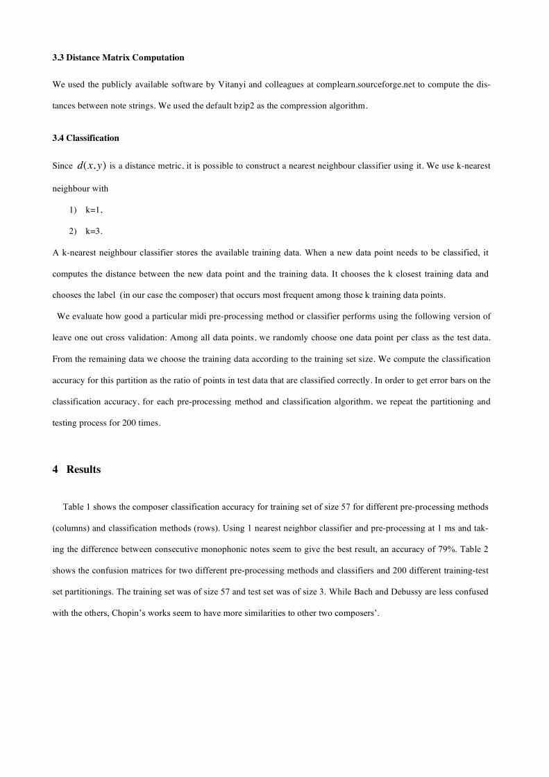
3.3 Distance Matrix Computation

We used the publicly available software by Vitanyi and colleagues at complearn.sourceforge.net to compute the dis-

tances between note strings. We used the default bzip2 as the compression algorithm.

3.4 Classification

Since

!

d(x,y) is a distance metric, it is possible to construct a nearest neighbour classifier using it. We use k-nearest

neighbour with

1) k=1,

2) k=3.

A k-nearest neighbour classifier stores the available training data. When a new data point needs to be classified, it

computes the distance between the new data point and the training data. It chooses the k closest training data and

chooses the label (in our case the composer) that occurs most frequent among those k training data points.

We evaluate how good a particular midi pre-processing method or classifier performs using the following version of

leave one out cross validation: Among all data points, we randomly choose one data point per class as the test data.

From the remaining data we choose the training data according to the training set size. We compute the classification

accuracy for this partition as the ratio of points in test data that are classified correctly. In order to get error bars on the

classification accuracy, for each pre-processing method and classification algorithm, we repeat the partitioning and

testing process for 200 times.

4 Results

Table 1 shows the composer classification accuracy for training set of size 57 for different pre-processing methods

(columns) and classification methods (rows). Using 1 nearest neighbor classifier and pre-processing at 1 ms and tak-

ing the difference between consecutive monophonic notes seem to give the best result, an accuracy of 79%. Table 2

shows the confusion matrices for two different pre-processing methods and classifiers and 200 different training-test

set partitionings. The training set was of size 57 and test set was of size 3. While Bach and Debussy are less confused

with the others, Chopin’s works seem to have more similarities to other two composers’.

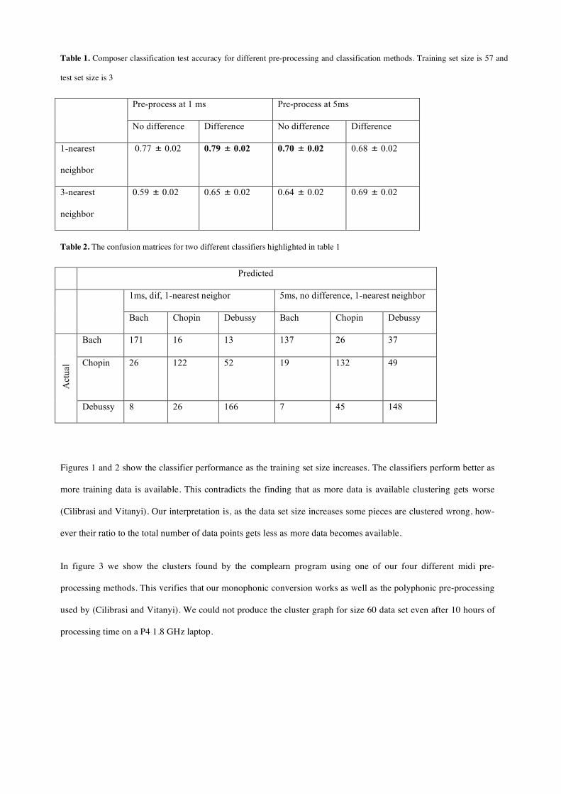
Table 1. Composer classification test accuracy for different pre-processing and classification methods. Training set size is 57 and

test set size is 3

Pre-process at 1 ms Pre-process at 5ms

No difference Difference No difference Difference

1-nearest

neighbor

0.77

!

± 0.02 0.79

!

± 0.02 0.70

!

± 0.02 0.68

!

± 0.02

3-nearest

neighbor

0.59

!

± 0.02 0.65

!

± 0.02 0.64

!

± 0.02 0.69

!

± 0.02

Table 2. The confusion matrices for two different classifiers highlighted in table 1

Predicted

1ms, dif, 1-nearest neighor 5ms, no difference, 1-nearest neighbor

Bach Chopin Debussy Bach Chopin Debussy

Bach 171 16 13 137 26 37

Chopin 26 122 52 19 132 49

Act

ual

Debussy 8 26 166 7 45 148

Figures 1 and 2 show the classifier performance as the training set size increases. The classifiers perform better as

more training data is available. This contradicts the finding that as more data is available clustering gets worse

(Cilibrasi and Vitanyi). Our interpretation is, as the data set size increases some pieces are clustered wrong, how-

ever their ratio to the total number of data points gets less as more data becomes available.

In figure 3 we show the clusters found by the complearn program using one of our four different midi pre-

processing methods. This verifies that our monophonic conversion works as well as the polyphonic pre-processing

used by (Cilibrasi and Vitanyi). We could not produce the cluster graph for size 60 data set even after 10 hours of

processing time on a P4 1.8 GHz laptop.

Fig. 1. The test classification accuracy for classical 60 data set at 1ms sampling. The classification accuracy

increases as the training set size increases. Using 1 nearest neighbor with difference pre-processing algorithm

performs best.

Fig. 2. The test classification accuracy for classical 60 data set at 5ms sampling. Again, the classification accu-

racy increases as the training set size increases. Using 1 nearest neighbor with difference pre-processing algo-

rithm still performs quite well. However the accuracy level is less than that of 1ms for all methods.

Fig. 3. The cluster produced by the complearn (complearn.sourceforge.net) program for the size 12 classical

data set using monophonic conversion and difference between time slices of 5ms.

5 Conclusion

In this paper we showed how the Kolmogorov distance measure and k-nearest neighbour classifier performs for

composer classification of midi files. We found out that the distance measure works better as more training data is

available. We also found out that, the distance metric may perform different with different input data pre-

processing methods.

Works Cited

Bishop, Christopher M., Neural Networks for Pattern Recognition, Oxford University Press, 1995.

Cilibrasi, Rudy, and P.M.B. Vitanyi, Clustering by compression, IEEE Trans. Inform. Th., 51:4(2005), 1523-1545.

Cilibrasi, Rudy, P.M.B Vitanyi and R. de Wolf, Algorithmic clustering of music based on string compression, Computer Music J.,

28:4(2004), 49-67.

Cover, Thomas. M., and J.A. Thomas, Elements of Information Theory, Wiley Interscience, 1991

Doraisamy, Shayamala, and S. Rüger, Robust Polyphonic Music Retrieval with N-grams, Journal of Intelligent Information

Systems, 21:1, 53–70, 2003.

Keogh, Eamonn, S. Lonardi, and C.A. Rtanamahatana, Toward parameter free data mining, Proc. 10th ACM SIGKDD Int. Conf.

Knowledge Discovery and Data Mining, Seattle, WA, Aug. 22–25, 2004, pp. 206–215.

Li, Ming, X. Chen, X. Li, B. Ma, and P.M.B. Vitanyi, The similarity metric, IEEE Trans. Inform. Th., 50:12(2004), 3250- 3264.

Li, Ming and R. Sleep, Melody classification using a similarity metric based on Kolmogorov Complexity, Sound and Music

Conference, 2004, Paris, France,

Uitdenbogerd, Alexandra L. and J. Zobel, Music Ranking Techniques Evaluated, Australian Computer Science Communications,

Vol 24, Issue 1, January-Fenruary 2002.