Embed Size (px)
Citation preview
MULTIVARIATE PRODUCTION SYSTEMS OPTIMIZATION
A REPORT
SUBMITTED TO THE DEPARTMENT OF PETROLEUM ENGINEERING
AND THE COMMITTEE ON GRADUATE STUDIES
OF STANFORD UNIVERSITY
IN PARTIAL FULFILLMENT OF THE REQUIREMENTS
FOR THE DEGREE OF
MASTER OF SCIENCE
By
James Aubrey Carroll, III
December, 1990

ii
Take heed you do not find what you do not seek.
[ English Proverb ]

iii
Approved for the Department:
Roland N. Horne
iv
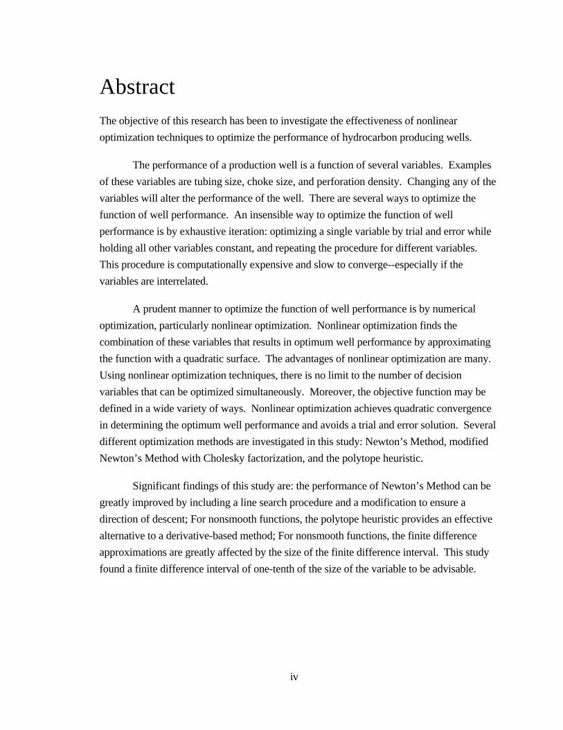
AbstractThe objective of this research has been to investigate the effectiveness of nonlinear
optimization techniques to optimize the performance of hydrocarbon producing wells.
The performance of a production well is a function of several variables. Examples
of these variables are tubing size, choke size, and perforation density. Changing any of the
variables will alter the performance of the well. There are several ways to optimize the
function of well performance. An insensible way to optimize the function of well
performance is by exhaustive iteration: optimizing a single variable by trial and error while
holding all other variables constant, and repeating the procedure for different variables.
This procedure is computationally expensive and slow to converge--especially if the
variables are interrelated.
A prudent manner to optimize the function of well performance is by numerical
optimization, particularly nonlinear optimization. Nonlinear optimization finds the
combination of these variables that results in optimum well performance by approximating
the function with a quadratic surface. The advantages of nonlinear optimization are many.
Using nonlinear optimization techniques, there is no limit to the number of decision
variables that can be optimized simultaneously. Moreover, the objective function may be
defined in a wide variety of ways. Nonlinear optimization achieves quadratic convergence
in determining the optimum well performance and avoids a trial and error solution. Several
different optimization methods are investigated in this study: Newton’s Method, modified
Newton’s Method with Cholesky factorization, and the polytope heuristic.
Significant findings of this study are: the performance of Newton’s Method can be
greatly improved by including a line search procedure and a modification to ensure a
direction of descent; For nonsmooth functions, the polytope heuristic provides an effective
alternative to a derivative-based method; For nonsmooth functions, the finite difference
approximations are greatly affected by the size of the finite difference interval. This study
found a finite difference interval of one-tenth of the size of the variable to be advisable.

v
AcknowledgementsI would like to thank Dr. Roland Horne for providing me with thoughtful guidance, sage
advice, and understanding patience. I also extend thanks to Dr. Khalid Aziz for providing
sound and judicious counsel and to Dr. Hank Ramey for his generous contributions.
I would like to thank Rafael Guzman for the time he invested proofreading several
drafts of this manuscript. I would also like to thank Cesar Palagi, Evandro Nacul,
Adalberto Rosa, Michael Riley, and Mariyamni Awang for providing a constant source of
quality advice. I would like to thank Russell Johns for providing experience in the drafting
of this manuscript. I would like to thank Suhail Qadeer and Daulat Mamora for helping me
with the computer hardware and David Brock and Chick Wattenbarger for being of
assistance with the computer graphics.
I would also like to express thanks to Dr. Walter Murray and Sam Eldersveld of the
Stanford Optimization Laboratory for their accessibility and helpfulness. I would like to
thank Dr. Jawahar Barua for writing a superb thesis that was instrumental in my fully
appreciating nonlinear concepts. I would like to thank Gunnar Borthne of the Norwegian
Institute of Technology and Godofredo Perez of the University of Tulsa for providing me
with computer programs that facilitated my work. I would also like to thank Joseph Gump
of Chevron, U.S.A., Gene Kouba of Chevron Exploration and Production Services, and
Dr. Rajesh Sachdeva of Simulation Sciences for providing me with a great deal of time and
help pertaining to system theory. I would like to thank Dr. Parvis Moin of NASA Ames
Research Center for inspiring my work by showing me the beauty and simplicity of
numerical methods.
I would like to express my sincere gratitude to Dr. Elias Schultzman and the
National Science Foundation for providing me with the financial capacity to pursue this
research. I would also like to thank the Stanford University Petroleum Research Institute
for providing resources and support.
Finally, I would like to thank the two most important people in the world, James
and Darlene Carroll, mom and dad, for giving me this opportunity.
vi
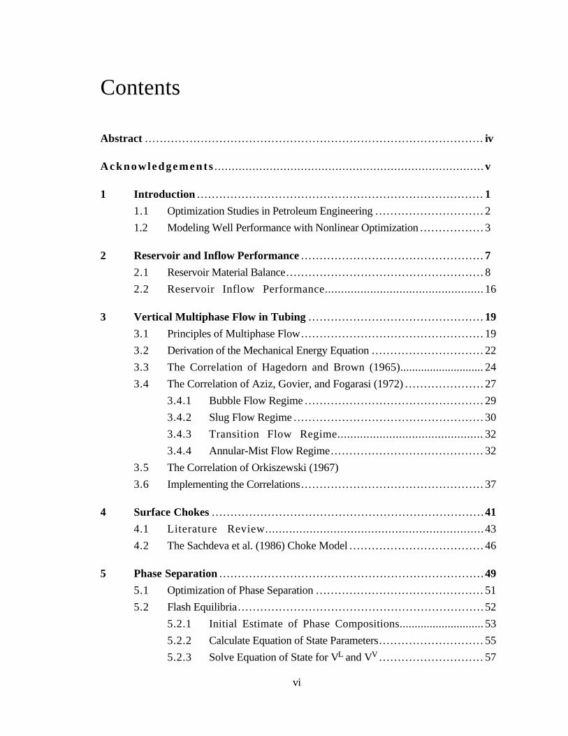
Contents
Abstract . . . . . . . . . . . . . . . . . . . . . . . . . . . . . . . . . . . . . . . . . . . . . . . . . . . . . . . . . . . . . . . . . . . . . . . . . . . . . . . . . . . . . . . . . . . iv
Acknowledgements .............................................................................. v
1 Introduction . . . . . . . . . . . . . . . . . . . . . . . . . . . . . . . . . . . . . . . . . . . . . . . . . . . . . . . . . . . . . . . . . . . . . . . . . . . . . 1
1.1 Optimization Studies in Petroleum Engineering .. . . . . . . . . . . . . . . . . . . . . . . . . . . . 2
1.2 Modeling Well Performance with Nonlinear Optimization .. . . . . . . . . . . . . . . . 3
2 Reservoir and Inflow Performance . . . . . . . . . . . . . . . . . . . . . . . . . . . . . . . . . . . . . . . . . . . . . . . . . 7
2.1 Reservoir Material Balance.. . . . . . . . . . . . . . . . . . . . . . . . . . . . . . . . . . . . . . . . . . . . . . . . . . . . 8
2.2 Reservoir Inflow Performance................................................. 16
3 Vertical Multiphase Flow in Tubing . . . . . . . . . . . . . . . . . . . . . . . . . . . . . . . . . . . . . . . . . . . . . . . 19
3.1 Principles of Multiphase Flow... . . . . . . . . . . . . . . . . . . . . . . . . . . . . . . . . . . . . . . . . . . . . . . 19
3.2 Derivation of the Mechanical Energy Equation .. . . . . . . . . . . . . . . . . . . . . . . . . . . . . 22
3.3 The Correlation of Hagedorn and Brown (1965)............................ 24
3.4 The Correlation of Aziz, Govier, and Fogarasi (1972) . . . . . . . . . . . . . . . . . . . . . 27
3.4.1 Bubble Flow Regime .. . . . . . . . . . . . . . . . . . . . . . . . . . . . . . . . . . . . . . . . . . . . . . . 29
3.4.2 Slug Flow Regime .. . . . . . . . . . . . . . . . . . . . . . . . . . . . . . . . . . . . . . . . . . . . . . . . . . 30
3.4.3 Transition Flow Regime............................................. 32
3.4.4 Annular-Mist Flow Regime.. . . . . . . . . . . . . . . . . . . . . . . . . . . . . . . . . . . . . . . . 32
3.5 The Correlation of Orkiszewski (1967)
3.6 Implementing the Correlations.. . . . . . . . . . . . . . . . . . . . . . . . . . . . . . . . . . . . . . . . . . . . . . . . 37
4 Surface Chokes . . . . . . . . . . . . . . . . . . . . . . . . . . . . . . . . . . . . . . . . . . . . . . . . . . . . . . . . . . . . . . . . . . . . . . . . . 41
4.1 Literature Review................................................................ 43
4.2 The Sachdeva et al. (1986) Choke Model . . . . . . . . . . . . . . . . . . . . . . . . . . . . . . . . . . . . 46
5 Phase Separation . . . . . . . . . . . . . . . . . . . . . . . . . . . . . . . . . . . . . . . . . . . . . . . . . . . . . . . . . . . . . . . . . . . . . . . 49
5.1 Optimization of Phase Separation .. . . . . . . . . . . . . . . . . . . . . . . . . . . . . . . . . . . . . . . . . . . . 51
5.2 Flash Equilibria.. . . . . . . . . . . . . . . . . . . . . . . . . . . . . . . . . . . . . . . . . . . . . . . . . . . . . . . . . . . . . . . . . 52
5.2.1 Initial Estimate of Phase Compositions............................ 53
5.2.2 Calculate Equation of State Parameters. . . . . . . . . . . . . . . . . . . . . . . . . . . . 55
5.2.3 Solve Equation of State for VL and VV .. . . . . . . . . . . . . . . . . . . . . . . . . . . 57
vii
5.2.4 Determine Partial Fugacities . . . . . . . . . . . . . . . . . . . . . . . . . . . . . . . . . . . . . . . . 58
5.2.5 Convergence Check.................................................. 58
5.2.6 Modify the Vapor and Liquid Compositions...................... 59
6 Nonlinear Optimization . . . . . . . . . . . . . . . . . . . . . . . . . . . . . . . . . . . . . . . . . . . . . . . . . . . . . . . . . . . . . . . 61
6.1 Newton’s Method .. . . . . . . . . . . . . . . . . . . . . . . . . . . . . . . . . . . . . . . . . . . . . . . . . . . . . . . . . . . . . . 63
6.2 Modifications to Newton’s Method .. . . . . . . . . . . . . . . . . . . . . . . . . . . . . . . . . . . . . . . . . . 68
6.2.1 The Method of Steepest Descent . . . . . . . . . . . . . . . . . . . . . . . . . . . . . . . . . . . 69
6.2.2 The Marquardt Modification .. . . . . . . . . . . . . . . . . . . . . . . . . . . . . . . . . . . . . . . 69
6.2.3 The Greenstadt Modification........................................ 70
6.3 Quasi-Newton Methods .. . . . . . . . . . . . . . . . . . . . . . . . . . . . . . . . . . . . . . . . . . . . . . . . . . . . . . . 71
6.4 The Polytope Algorithm ... . . . . . . . . . . . . . . . . . . . . . . . . . . . . . . . . . . . . . . . . . . . . . . . . . . . . . 72
7 Results . . . . . . . . . . . . . . . . . . . . . . . . . . . . . . . . . . . . . . . . . . . . . . . . . . . . . . . . . . . . . . . . . . . . . . . . . . . . . . . . . . . . 77
7.1 Model Development.. . . . . . . . . . . . . . . . . . . . . . . . . . . . . . . . . . . . . . . . . . . . . . . . . . . . . . . . . . . . 77
7.1.1 Developing a Well Model Prototype .. . . . . . . . . . . . . . . . . . . . . . . . . . . . . . 77
7.1.2 Developing the Reservoir Component. . . . . . . . . . . . . . . . . . . . . . . . . . . . . 81
7.1.3 Developing the Tubing Component. . . . . . . . . . . . . . . . . . . . . . . . . . . . . . . . 81
7.1.4 Developing the Choke Component................................. 88
7.1.5 Developing the Separation Component. . . . . . . . . . . . . . . . . . . . . . . . . . . . 89
7.2 Defining the Objective Criterion .. . . . . . . . . . . . . . . . . . . . . . . . . . . . . . . . . . . . . . . . . . . . . . 89
7.3 Results. . . . . . . . . . . . . . . . . . . . . . . . . . . . . . . . . . . . . . . . . . . . . . . . . . . . . . . . . . . . . . . . . . . . . . . . . . . . 94
7.3.1 The Surface of the Well Model . . . . . . . . . . . . . . . . . . . . . . . . . . . . . . . . . . . . . 94
7.3.2 Performing Optimization on the Well Model...................... 106
8 Conclusions . . . . . . . . . . . . . . . . . . . . . . . . . . . . . . . . . . . . . . . . . . . . . . . . . . . . . . . . . . . . . . . . . . . . . . . . . . . . . . 117
8.1 Conclusions.. . . . . . . . . . . . . . . . . . . . . . . . . . . . . . . . . . . . . . . . . . . . . . . . . . . . . . . . . . . . . . . . . . . . . 117
8.2 Suggestions for Future Work.. . . . . . . . . . . . . . . . . . . . . . . . . . . . . . . . . . . . . . . . . . . . . . . . . 118
N o m e n c l a t u r e ..................................................................................... 121
Bibliography . . . . . . . . . . . . . . . . . . . . . . . . . . . . . . . . . . . . . . . . . . . . . . . . . . . . . . . . . . . . . . . . . . . . . . . . . . . . . . . . . . . . . . 125
Appendix Source Code for Well Model . . . . . . . . . . . . . . . . . . . . . . . . . . . . . . . . . . . . . . . . . . . . . . . . 133

viii
List of Tables
Table 3.1 Correlating Functions of Hagedorn and Brown (1965). . . . . . . . . . . . . . . . . . . . 25
Table 4.1 Empirical Coefficients for Two-Phase Critical Flow Correlations. . . . . . . . 45
Table 5.1 Binary Interaction Parameters for the Soave Equation.. . . . . . . . . . . . . . . . . . . . . 56
ix
List of Figures
Figure 1.1 Graphical Examples of Nodal Analysis. . . . . . . . . . . . . . . . . . . . . . . . . . . . . . . . . . . . . . . . . . . . . . . . . . 4
Figure 1.2 Schematic of a Well Model. . . . . . . . . . . . . . . . . . . . . . . . . . . . . . . . . . . . . . . . . . . . . . . . . . . . . . . . . . . . . . . . 4
Figure 2.1 Phase Behavior Assumptions of Reservoir Material Balance Procedure............. 9
Figure 3.1 Flow Regimes of Aziz, Govier, and Fogarasi (1972).................................. 28
Figure 3.2 Flow-Pattern Map Proposed by Aziz, Govier, and Fogarasi (1972).. . . . . . . . . . . . . . . . 29
Figure 3.3 Flow-Pattern Map Proposed by Orkiszewski (1967). . . . . . . . . . . . . . . . . . . . . . . . . . . . . . . . . . 35
Figure 3.4 Pressure Traverse Flow Diagram... . . . . . . . . . . . . . . . . . . . . . . . . . . . . . . . . . . . . . . . . . . . . . . . . . . . . . . 39
Figure 4.1 Positive Choke.. . . . . . . . . . . . . . . . . . . . . . . . . . . . . . . . . . . . . . . . . . . . . . . . . . . . . . . . . . . . . . . . . . . . . . . . . . . . . 41
Figure 4.2 Mass Flow Rate versus Pressure Ratio. . . . . . . . . . . . . . . . . . . . . . . . . . . . . . . . . . . . . . . . . . . . . . . . . . 43
Figure 4.3 Real and Spurious Roots of the Mass Flux Residual................................... 48
Figure 5.1 Schematic of Horizontal Separator. . . . . . . . . . . . . . . . . . . . . . . . . . . . . . . . . . . . . . . . . . . . . . . . . . . . . . . 49
Figure 5.2 Stage Separation. . . . . . . . . . . . . . . . . . . . . . . . . . . . . . . . . . . . . . . . . . . . . . . . . . . . . . . . . . . . . . . . . . . . . . . . . . . . 50
Figure 5.3 Effect of Separator Pressure in a Two-Stage Separation Process..................... 52
Figure 6.1 A Maximum and a Minimum... . . . . . . . . . . . . . . . . . . . . . . . . . . . . . . . . . . . . . . . . . . . . . . . . . . . . . . . . . . . 62
Figure 6.2 Discretization Scheme Used for Finite Difference Approximations .. . . . . . . . . . . . . . . . . 67
Figure 6.3 Two-Dimensional Polytope. . . . . . . . . . . . . . . . . . . . . . . . . . . . . . . . . . . . . . . . . . . . . . . . . . . . . . . . . . . . . . . 75
Figure 7.1 Flow Rate Surface of Single-Phase Model, 3-D. . . . . . . . . . . . . . . . . . . . . . . . . . . . . . . . . . . . . . . . 78
Figure 7.2 Flow Rate Surface of Single-Phase Model, 2-D. . . . . . . . . . . . . . . . . . . . . . . . . . . . . . . . . . . . . . . . 79
Figure 7.3 Convergence Path of Single-Phase Model............................................... 80
Figure 7.4 Hagedorn and Brown Gradient Map, 2-D... . . . . . . . . . . . . . . . . . . . . . . . . . . . . . . . . . . . . . . . . . . . . 82
Figure 7.5 Hagedorn and Brown Gradient Map, 3-D... . . . . . . . . . . . . . . . . . . . . . . . . . . . . . . . . . . . . . . . . . . . . 83
Figure 7.6 Aziz, Govier, and Fogarasi Gradient Map, 2-D. .. . . . . . . . . . . . . . . . . . . . . . . . . . . . . . . . . . . . . . 84
Figure 7.7 Aziz, Govier, and Fogarasi Gradient Map, 3-D. .. . . . . . . . . . . . . . . . . . . . . . . . . . . . . . . . . . . . . . 85
Figure 7.8 Orkiszewski Gradient Map, 2-D... . . . . . . . . . . . . . . . . . . . . . . . . . . . . . . . . . . . . . . . . . . . . . . . . . . . . . . . 86
Figure 7.9 Orkiszewski Gradient Map, 3-D... . . . . . . . . . . . . . . . . . . . . . . . . . . . . . . . . . . . . . . . . . . . . . . . . . . . . . . . 87
Figure 7.10 Present Value Surface of Choke Diameter vs. Tubing Diameter.. . . . . . . . . . . . . . . . . . . . . 90
Figure 7.11 Constrained Present Value Surface of Choke Diameter vs. Tubing Diameter. . . . . . . 91
Figure 7.12 Revenue Stream is Discounted from Center of Time Step. . . . . . . . . . . . . . . . . . . . . . . . . . . . . 93
Figure 7.13 Present Value Surface of Separator Pressure vs. Tubing Diameter................... 95
Figure 7.14 Rough Features of Present Value Surface. . . . . . . . . . . . . . . . . . . . . . . . . . . . . . . . . . . . . . . . . . . . . . . 96
Figure 7.15 Profile of Tubing Diameter for Constant Separator Pressure.......................... 97
Figure 7.16 Close-up of Tubing Diameter Profile for Constant Separator Pressure. . . . . . . . . . . . . . 98

x
Figure 7.17 Close-up of Tubing Diameter Profile at Optimum. .. . . . . . . . . . . . . . . . . . . . . . . . . . . . . . . . . . . . 99
Figure 7.18 Profile of Separator Pressure for Constant Tubing Diameter.......................... 100
Figure 7.19 First Derivative of Separator Pressure. . . . . . . . . . . . . . . . . . . . . . . . . . . . . . . . . . . . . . . . . . . . . . . . . . . 101
Figure 7.20 Second Derivative of Separator Pressure. . . . . . . . . . . . . . . . . . . . . . . . . . . . . . . . . . . . . . . . . . . . . . . . 102
Figure 7.21 First Derivative of Tubing Diameter. . . . . . . . . . . . . . . . . . . . . . . . . . . . . . . . . . . . . . . . . . . . . . . . . . . . . . 103
Figure 7.22 Second Derivative of Tubing Diameter................................................... 104
Figure 7.23 Mixed-Partial Derivative of Tubing Diameter and Separator Pressure. . . . . . . . . . . . . . . 105
Figure 7.24 Minimum Eigenvalue of Hessian Matrix................................................. 107
Figure 7.25 Maximum Eigenvalue of Hessian Matrix. . . . . . . . . . . . . . . . . . . . . . . . . . . . . . . . . . . . . . . . . . . . . . . . 108
Figure 7.26 Curvature of Hessian Matrix. . . . . . . . . . . . . . . . . . . . . . . . . . . . . . . . . . . . . . . . . . . . . . . . . . . . . . . . . . . . . . 109
Figure 7.27 Convergence Path of Unmodified Newton’s Method.. . . . . . . . . . . . . . . . . . . . . . . . . . . . . . . . . 111
Figure 7.28 Convergence Path of Modified Newton’s Method. . . . . . . . . . . . . . . . . . . . . . . . . . . . . . . . . . . . . 112
Figure 7.29 Convergence Path of Polytope Heuristic, 2-D. .. . . . . . . . . . . . . . . . . . . . . . . . . . . . . . . . . . . . . . . . 113
Figure 7.30 Convergence Path of Polytope Heuristic, 3-D. .. . . . . . . . . . . . . . . . . . . . . . . . . . . . . . . . . . . . . . . . 114
Figure 7.31 Convergence Path of Triangular Polytopes.............................................. 115

1
Chapter 1
INTRODUCTION
The performance of a production well is a function of several variables.
Q = f Pres, Dtubing, Dchoke, Dflowline, Psep, ... (1.1)
A change in any one of the variables will cause a change in the performance of the well.
When designing a new well, or when analyzing an existing well, an engineer will attempt
to determine the combination of variables under his or her control that produces the “best”
performance of the well. A common procedure to determine the optimal combination of
these variables is to develop a model of the well and then use some form of trial and error
procedure until the engineer feels that the optimal mix of variables has been determined. In
addition to being quite expensive computationally, no certainty can be had that this is the
optimal mix of variables as opposed to just a good mix of variables. Fortunately,
mathematical techniques are available to determine the optimal mix of these variables
without performing a trial and error procedure.
Mathematically, optimization involves finding the extreme values of a function.
Given a function of several variables,
Z = f x1, x2, x3, , xn (1.2)
an optimization scheme will find the combination of these variables that produces an
extreme value in the function, be it a minimum value or a maximum value. There are many
examples of optimization. For example, if a function gives an investor’s expected return as
a function of different investments, numerical optimization of the function will determine
the mix of investments that will yield the maximum expected return. This is the basis of
modern portfolio theory. If a function gives the difference between a set of data and a
model of the data, numerical optimization of the function will produce the best fit of the
model to the data. This is the basis for nonlinear parameter estimation. Similar examples
can be given for network analysis, queueing theory, decision analysis, etc.
Optimization has historically been used in the petroleum industry to allocate
production through pipeline networks, to schedule transoceanic shipments of petroleum

2
from supply sites to demand sites, to model refinery throughput, and to determine the best
use of limited amounts of capital. Lasdon et al. (1986) point out that the production sector
of the petroleum industry has seen few successful applications of optimization methods.
The objective of this research has been to investigate the effectiveness of nonlinear
optimization techniques to optimize the performance of hydrocarbon producing wells.
The study consisted of two primary phases: 1) development of a well model that determines
well performance, and 2) optimization of well performance with nonlinear optimization
techniques.
1.1 Optimization Studies in Petroleum Engineering
Optimization methodologies are the focus of the field of Operations Research, a field that
has only been in existence since the 1940’s. Operations Research concepts were not
adopted by the petroleum industry until the early 1950’s. The bulk of the literature since
then has been on linear programming techniques applied to reservoir management on a
macro-level. For a detailed treatment of optimization methods in petroleum engineering,
see Aronofsky (1983).
Aronofsky and Lee (1958) developed a linear programming model to maximize
profit by scheduling production from multiple single-well reservoirs. Aronofsky and
Williams (1962) extended the same model to investigate the problems of scheduling
production for a fixed drilling program and also scheduling drilling for a fixed production
schedule. Charnes and Cooper (1961) used linear programming to develop a reservoir
model that minimized the cost of wells and facilities subject to a constant production
schedule. Attra et al. (1961) developed a linear programming model to maximize flow rate
subject to several production constraints. All of these models used linear reservoir models
based on material balance considerations, and the reservoirs were generally assumed
uniform and single phase.
Rowan and Warren (1967) demonstrated how to formulate the reservoir
management problem in terms of optimal control theory. Bohannon (1970) used a mixed-
integer linear programming model to optimize a pipeline network. O’Dell et al. (1973)
developed a linear programming model to optimize production scheduling from a
multireservoir system. Huppler (1974) developed a dynamic programming model to
optimize well and facility design given the delivery schedule and using a material balance
3
reservoir model. Kuller and Cummings (1974) developed an economic linear
programming model of production and investment for petroleum reservoirs.
Several investigators have attempted to couple numerical reservoir simulation with
linear programming models. The idea has been to use the reservoir simulator to generate a
linearized unit response matrix that could be used with linear programming models.
Wattenbarger (1970) developed a linear programming model to schedule production from a
gas storage reservoir using this technique. Rosenwald and Green (1974) also used
influence functions in a mixed-integer linear programming model that optimized well
placement. Murray and Edgar (1979) used influence functions in a mixed-integer linear
programming model that optimized well placement and production scheduling. See and
Horne (1983), extending on work performed by Coats (1969) and Crichlow (1977),
demonstrated how to refine the unit response matrix using nonlinear regression techniques.
This work was expanded by Lang and Horne (1983) to consider dynamic programming
techniques.
Asheim (1978) studied petroleum developments in the North Sea by coupling
reservoir simulation and optimization. Ali et al. (1983) used nonlinear programming to
study reservoir development and investment policies in Kuwait. McFarland et al. (1984)
used nonlinear optimization to optimize reservoir production scheduling.
Notice that virtually all of the previous research has attempted to model reservoir
performance by linearizing the reservoir performance and feeding this to some variation of
linear programming. The main focus in every case was to model the reservoir
performance. None of the models endeavored to optimize the well performance.
1.2 Modeling Well Performance with Nonlinear Optimization
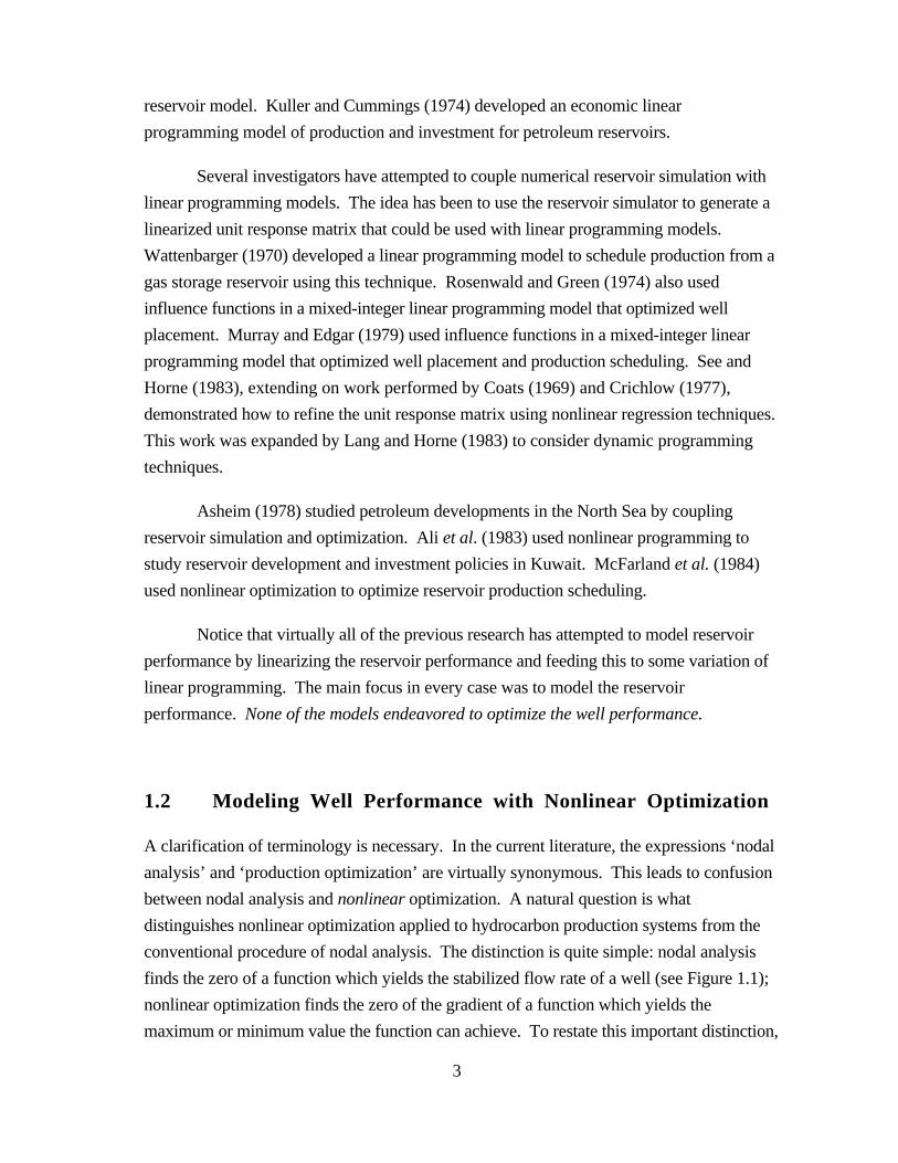
A clarification of terminology is necessary. In the current literature, the expressions ‘nodal
analysis’ and ‘production optimization’ are virtually synonymous. This leads to confusion
between nodal analysis and nonlinear optimization. A natural question is what
distinguishes nonlinear optimization applied to hydrocarbon production systems from the
conventional procedure of nodal analysis. The distinction is quite simple: nodal analysis
finds the zero of a function which yields the stabilized flow rate of a well (see Figure 1.1);
nonlinear optimization finds the zero of the gradient of a function which yields the
maximum or minimum value the function can achieve. To restate this important distinction,
4
Flow Rate Q*
PressureatSolutionNode
Reservoir Performance Curve
Tubing Performance Curve
PressureDifferentialatSolutionNode
0
Root ofFunction
Stabilized ConditionsP*
Flow Rate Q*
Figure 1.1: Graphical Examples of Nodal Analysis.
Reservoir Model
Tubing Model
ChokeModel
Separator Model
Input:Tubing Size
Input:Choke Size
Input:SeparatorPressure
Output:Oil Flow Rate
Figure 1.2: Schematic of a Well Model.
nodal analysis finds a solution by locating the zero of a function; nonlinear optimization
finds the optimum solution by locating the zero of the gradient of an objective function.
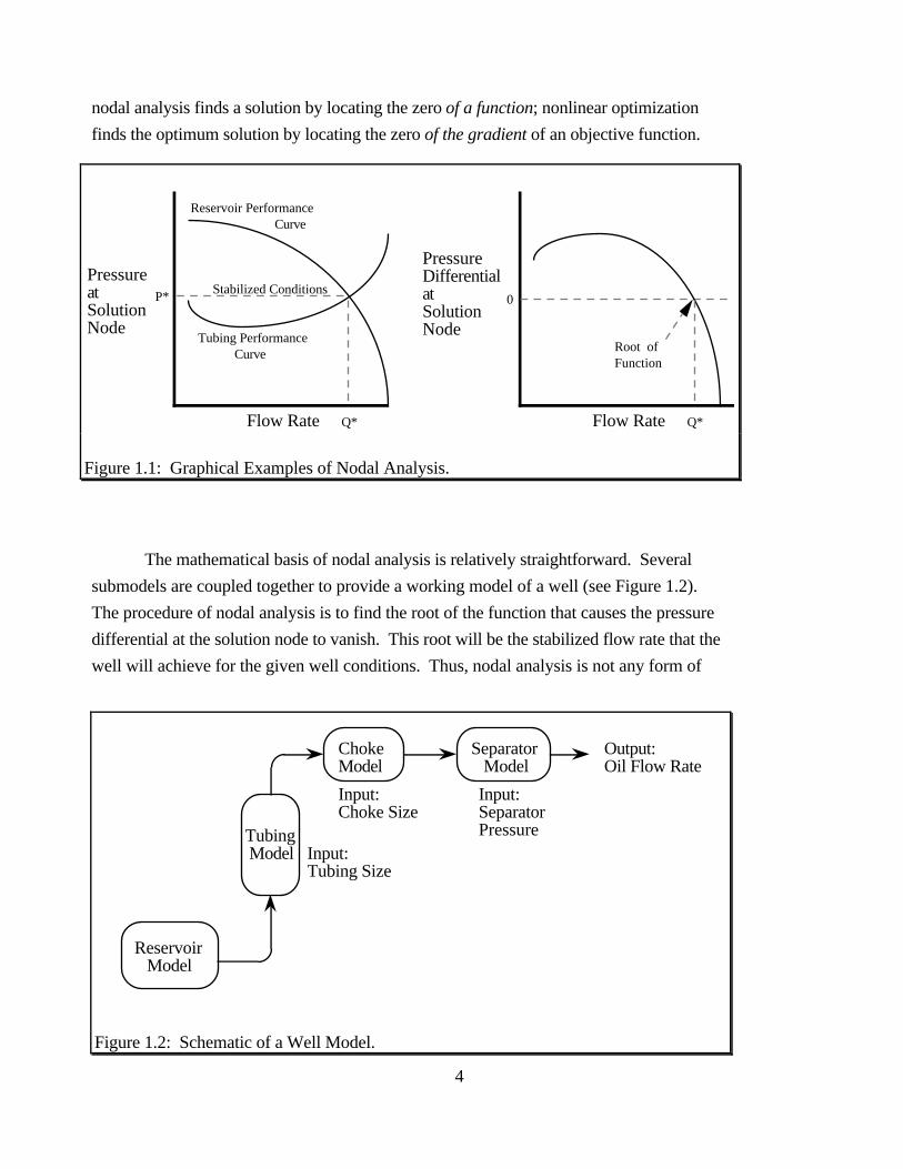
The mathematical basis of nodal analysis is relatively straightforward. Several
submodels are coupled together to provide a working model of a well (see Figure 1.2).
The procedure of nodal analysis is to find the root of the function that causes the pressure
differential at the solution node to vanish. This root will be the stabilized flow rate that the
well will achieve for the given well conditions. Thus, nodal analysis is not any form of
5
optimization, it is merely the procedure of finding the stabilized flow rate that satisfies the
function of well performance. The confusion with optimization arises because some people
will use nodal analysis in an exhaustive manner to optimize a single variable ( e.g., tubing
diameter). By holding all other parameters constant, a single parameter is varied to see
where the maximum stabilized flow rate will occur. For more information on nodal
analysis and ‘production systems optimization’, see Brown (1977), Chu (1983), Brown
and Lea (1985), Golan and Whitson (1986), Lea and Brown (1986), and Hunt (1988).
It is trivial to optimize a function of a single variable: simply plot the variable
against the objective criterion and take the extreme value. A single performance curve is all
that is required. Matters become complicated if a function of several variables is to be
optimized, particularly if the variables are interrelated. To optimize a function of two
variables, a performance curve of the first variable plotted against the objective criterion is
required for every discrete value of the second variable. The single performance curve
required to optimize one variable balloons into a family of performance curves when two
variables are optimized. If three variables are optimized, a family of performance curves is
required for every discrete value of the third variable. This manner of optimization rapidly
becomes intractable because it suffers from the curse of dimensionality--the work involved
increases rapidly as additional dimensions are added. This is when the potency of
numerical optimization becomes very obvious.
Using nonlinear optimization techniques, there is no limit to the number of decision
variables that can be optimized concurrently. All that is required is an objective function
that takes all of the decision variables as input and determines the objective variable.
Examples of different objective functions are numerous: to maximize the present value of
the production stream, to maximize the net present value of the well, to maximize
cumulative recovery on an equivalent barrel basis, to minimize the cumulative gas-oil ratio,
to minimize the cumulative water-oil ratio, to minimize total investment per equivalent
barrel produced, to maximize the rate-of-return of the well, and so on.
As previously mentioned, the study consisted of two primary phases: 1)
development of a well model that determines well performance, and 2) optimization of well
performance with nonlinear optimization techniques. Chapters 2 through 5 discuss the
intricacies involved in the design and development of the various components of the well
model as follows: Chapter 2 discusses reservoir material balance and inflow performance,
Chapter 3 discusses multiphase flow through vertical tubing, Chapter 4 discusses
multiphase flow through surface chokes, and Chapter 5 discusses the separation facilities.

6
Chapters 6 through 8 discuss the integration of the well model with the nonlinear
optimization methods and the conclusions that were drawn. Chapter 6 discusses the theory
and implementation of nonlinear optimization techniques. Chapter 7 describes the results
of optimizing the well model with various types of nonlinear optimization techniques.
Chapter 8 concludes the report by discussing significant findings and proposing ideas for
future research.
7
Chapter 2
RESERVOIR AND INFLOW PERFORMANCE
To replicate the reservoir and inflow performance of a hydrocarbon production system, this
study adopted a reservoir model developed by Borthne (1986) at the Norwegian Institute of
Technology. The model was originally designed with just this purpose in mind--to provide
a simple but functional reservoir component to be included in a larger model. The model
provides an accurate representation of constrained reservoir performance that requires
minimal computer processing. Since the model was to be used in an optimization study
that would require numerous function evaluations, the speed of the model was important.
Borthne’s (1986) model is a black-oil model that performs a generalized material
balance calculation in concert with an inflow performance relationship based on
pseudopressure. The model derives its processing speed from making several simplifying
assumptions. Some of the major assumptions are:
• The reservoir is homogeneous, isotropic, horizontal, cylindrical, and of
uniform thickness;
• The reservoir is a zero-dimensional single cell that is bounded by no-flow
boundaries;
• The reservoir is initially saturated with a single phase fluid--either oil
above the bubble point or gas above the dew point--and immobile connate
water;
• The reservoir drive mechanism is solution-gas drive for oil and depletion
drive for gas;
• The producing gas-oil ratio is constant throughout the reservoir;
• Production occurs under pseudosteady state conditions and at a constant
rate;
• Capillary pressure, gravity effects, and coning are negligible.
8
The reservoir model is constrained by both pressure and flowrate. In addition to specifying
a minimum flowing well pressure, two flowrates must be specified: a minimum flowrate
and a maximum target flowrate. The model attempts to satisfy the target flowrate without
violating the minimum flowing well pressure.
2.1 Reservoir Material Balance
Reproduced here is the theory and procedure of the “generalized” material balance method
as implemented in the reservoir model developed by Borthne (1986). For a more
exhaustive treatment on the subject, the reader is referred to Borthne’s thesis.
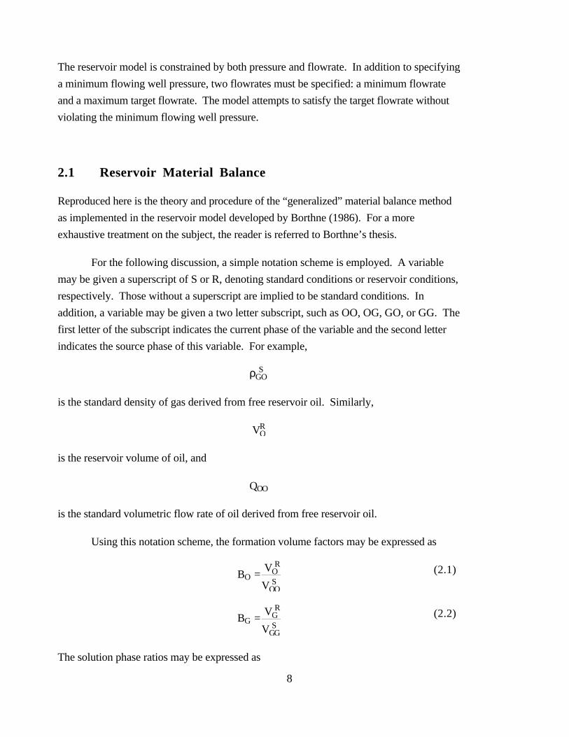
For the following discussion, a simple notation scheme is employed. A variable
may be given a superscript of S or R, denoting standard conditions or reservoir conditions,
respectively. Those without a superscript are implied to be standard conditions. In
addition, a variable may be given a two letter subscript, such as OO, OG, GO, or GG. The
first letter of the subscript indicates the current phase of the variable and the second letter
indicates the source phase of this variable. For example,
ρGOS
is the standard density of gas derived from free reservoir oil. Similarly,
VOR
is the reservoir volume of oil, and
QOO
is the standard volumetric flow rate of oil derived from free reservoir oil.
Using this notation scheme, the formation volume factors may be expressed as
BO = VO
R
VOOS
(2.1)
BG = VG
R
VGGS
(2.2)
The solution phase ratios may be expressed as
9
RS = VGO
S
VOOS
(2.3)
rS = VOG
S
VGGS
(2.4)
where
RS is the solution gas-oil ratio
rS is the solution oil-gas ratio
It should be made clear that the model allows both phases to contain the other phase in
solution as shown in Figure 2.1.
Surface Oil
Reservoir Oil
Surface Gas
Reservoir Gas
Figure 2.1: Phase Behavior Assumptions of Reservoir Material Balance Procedure.
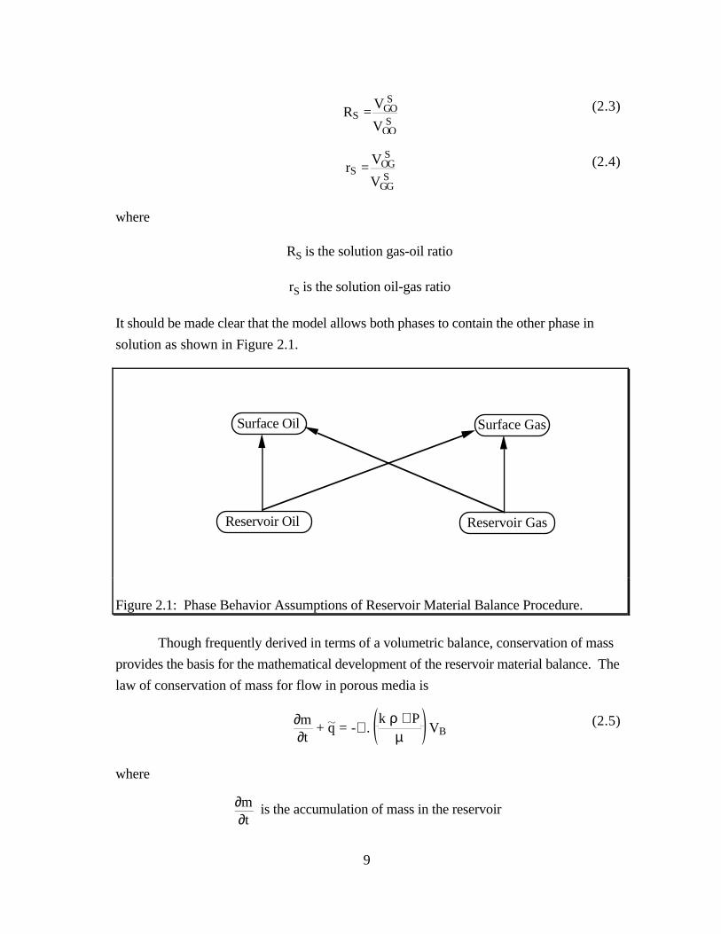
Though frequently derived in terms of a volumetric balance, conservation of mass
provides the basis for the mathematical development of the reservoir material balance. The
law of conservation of mass for flow in porous media is
∂m∂t
+ q = -∇ . k ρ ∇ P
µ VB
(2.5)
where
∂m∂t
is the accumulation of mass in the reservoir

10
q is the mass production rate from the reservoir, the source-sink term, and
∇ . k ρ ∇ P
µ VB
is the mass flux term across the reservoir boundaries.
A material balance considers the reservoir to be a single cell with no-flow boundaries.
Therefore the mass flux term is zero and the equation simplifies to
∂m∂t
+ q = 0 (2.6)
Discretizing and multiplying by a time interval ∆t yields
∆m + q ∆t = 0 (2.7)
which simply states that the change of fluid mass in the reservoir must be equivalent to the
mass of fluid that was produced or injected.
Equation 2.7 consists of a mass accumulation term and mass source-sink term. The
accumulation term consists of the change in the mass of the reservoir fluids over time. The
fluid mass in the reservoir at any given time (implied standard conditions) may be given as
mO = mOO + mOG (2.8)
mG = mGG + mGO
where
mOO = φ SO ρOO
S
BO VB
(2.9)
mOG = φ SG ρOG
S
BG VB
(2.10)
mGG = φ SG ρGG
S
BG VB
(2.11)
mGO = φ SO ρGO
S
BO VB
(2.12)
11
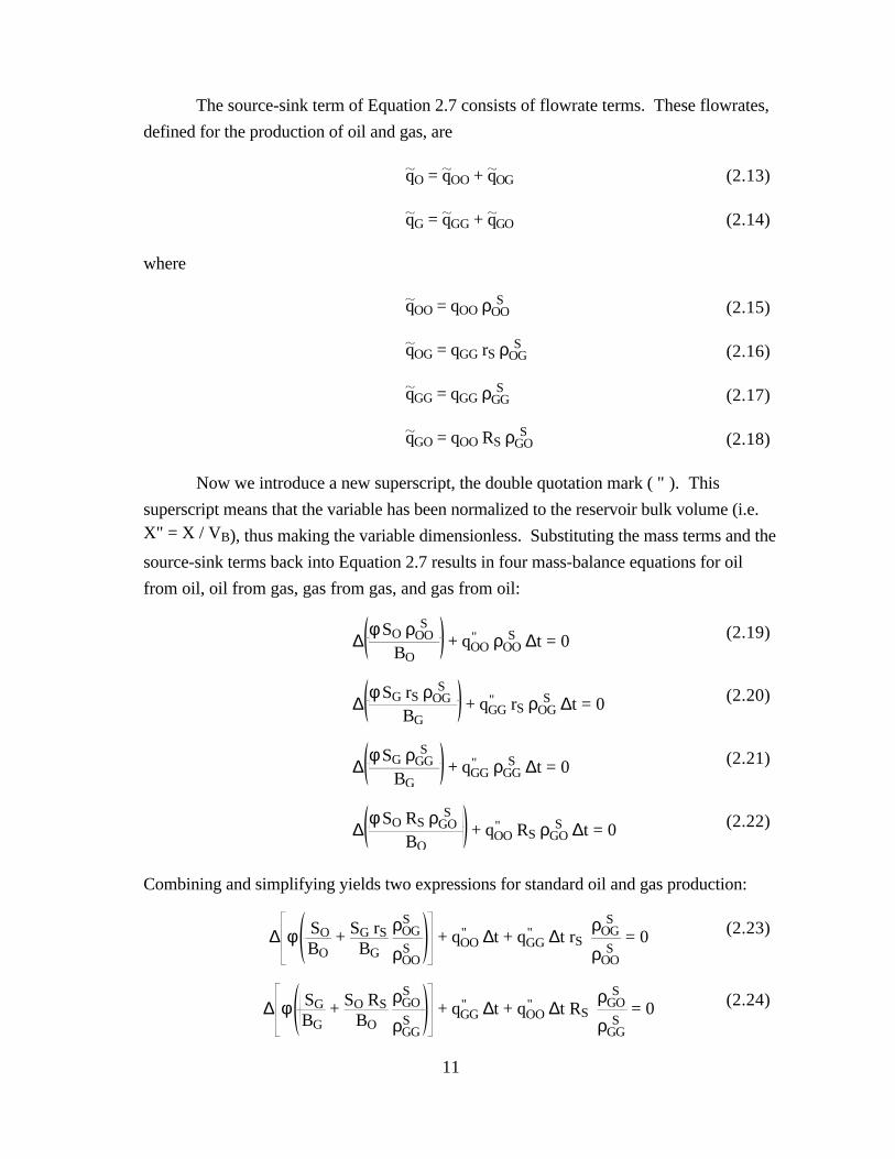
The source-sink term of Equation 2.7 consists of flowrate terms. These flowrates,
defined for the production of oil and gas, are
qO = qOO + qOG (2.13)
qG = qGG + qGO (2.14)
where
qOO = qOO ρOOS (2.15)
qOG = qGG rS ρOGS (2.16)
qGG = qGG ρGGS (2.17)
qGO = qOO RS ρGOS (2.18)
Now we introduce a new superscript, the double quotation mark ( " ). This
superscript means that the variable has been normalized to the reservoir bulk volume (i.e.X" = X / VB), thus making the variable dimensionless. Substituting the mass terms and the
source-sink terms back into Equation 2.7 results in four mass-balance equations for oil
from oil, oil from gas, gas from gas, and gas from oil:
∆φ SO ρOO
S BO
+ qOO" ρOO
S ∆t = 0 (2.19)
∆φ SG rS ρOG
S BG
+ qGG" rS ρOG
S ∆t = 0 (2.20)
∆φ SG ρGG
S BG
+ qGG" ρGG
S ∆t = 0 (2.21)
∆φ SO RS ρGO
S BO
+ qOO" RS ρGO
S ∆t = 0 (2.22)
Combining and simplifying yields two expressions for standard oil and gas production:
∆ φ SOBO
+ SG rSBG
ρOG
S
ρOOS
+ qOO" ∆t + qGG
" ∆t rS ρOG
S
ρOOS
= 0 (2.23)
∆ φ SGBG
+ SO RSBO
ρGO
S
ρGGS
+ qGG" ∆t + qOO
" ∆t RS ρGO
S
ρGGS
= 0 (2.24)
12
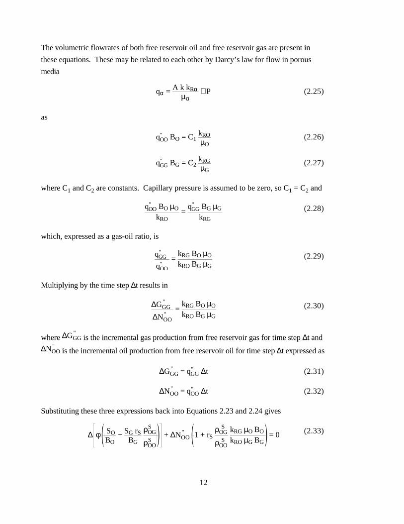
The volumetric flowrates of both free reservoir oil and free reservoir gas are present in
these equations. These may be related to each other by Darcy’s law for flow in porous
media
qα = A k kRαµα
∇ P (2.25)
as
qOO" BO = C1 kRO
µO(2.26)
qGG" BG = C2 kRG
µG(2.27)
where C1 and C2 are constants. Capillary pressure is assumed to be zero, so C1 = C2 and
qOO" BO µO
kRO =
qGG" BG µG
kRG
(2.28)
which, expressed as a gas-oil ratio, is
qGG"
qOO"
= kRG BO µO
kRO BG µG
(2.29)
Multiplying by the time step ∆t results in
∆GGG"
∆NOO"
= kRG BO µO
kRO BG µG
(2.30)
where ∆GGG"
is the incremental gas production from free reservoir gas for time step ∆t and
∆NOO"
is the incremental oil production from free reservoir oil for time step ∆t expressed as
∆GGG" = qGG
" ∆t (2.31)
∆NOO" = qOO
" ∆t (2.32)
Substituting these three expressions back into Equations 2.23 and 2.24 gives
∆ φ SOBO
+ SG rSBG
ρOG
S
ρOOS
+ ∆NOO" 1 + rS
ρOGS
ρOOS
kRG µO BO
kRO µG BG = 0 (2.33)
13
∆ φ SGBG
+ SO RSBO
ρGO
S
ρGGS
+ ∆NOO"
kRG µO BO
kRO µG BG + RS
ρGOS
ρGGS
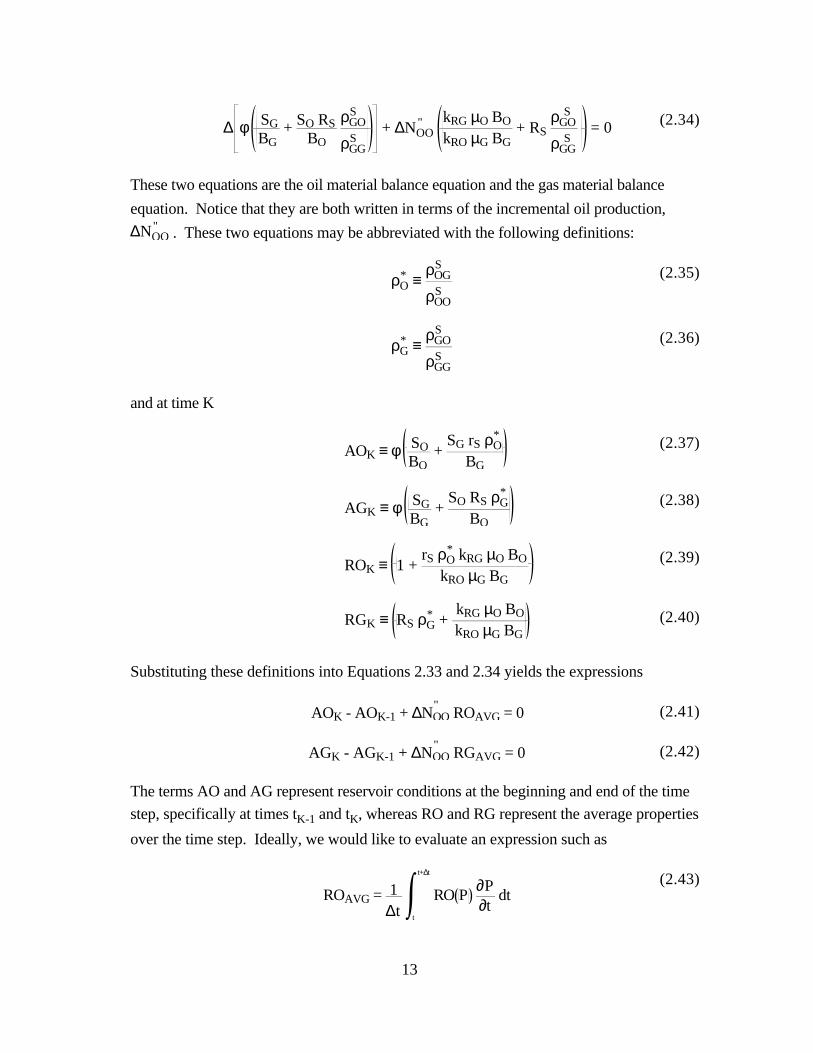
= 0 (2.34)
These two equations are the oil material balance equation and the gas material balance
equation. Notice that they are both written in terms of the incremental oil production,
∆NOO" . These two equations may be abbreviated with the following definitions:
ρO* ≡
ρOGS
ρOOS
(2.35)
ρG* ≡
ρGOS
ρGGS
(2.36)
and at time K
AOK ≡ φ SOBO
+ SG rS ρO
*
BG (2.37)
AGK ≡ φ SGBG
+ SO RS ρG
*
BO (2.38)
ROK ≡ 1 + rS ρO
* kRG µO BO
kRO µG BG
(2.39)
RGK ≡ RS ρG* +
kRG µO BO
kRO µG BG(2.40)
Substituting these definitions into Equations 2.33 and 2.34 yields the expressions
AOK - AOK-1 + ∆NOO"
ROAVG = 0 (2.41)
AGK - AGK-1 + ∆NOO"
RGAVG = 0 (2.42)
The terms AO and AG represent reservoir conditions at the beginning and end of the time
step, specifically at times tK-1 and tK, whereas RO and RG represent the average properties
over the time step. Ideally, we would like to evaluate an expression such as
ROAVG = 1∆t
RO Pt
t+∆t
∂P∂t
dt(2.43)
14
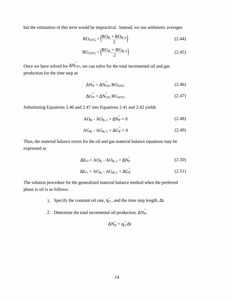
but the estimation of this term would be impractical. Instead, we use arithmetic averages
ROAVG = ROK + ROK-12
(2.44)
RGAVG = RGK + RGK-12
(2.45)
Once we have solved for ∆NOO"
, we can solve for the total incremental oil and gas
production for the time step as
∆NP" = ∆NOO
" ROAVG (2.46)
∆GP" = ∆NOO
" RGAVG (2.47)
Substituting Equations 2.46 and 2.47 into Equations 2.41 and 2.42 yields
AOK - AOK-1 + ∆NP" = 0 (2.48)
AGK - AGK-1 + ∆GP" = 0 (2.49)
Thus, the material balance errors for the oil and gas material balance equations may be
expressed as
∆EO = AOK - AOK-1 + ∆NP" (2.50)
∆EG = AGK - AGK-1 + ∆GP" (2.51)
The solution procedure for the generalized material balance method when the preferred
phase is oil is as follows:
1. Specify the constant oil rate, qO" , and the time step length, ∆t.
2. Determine the total incremental oil production, ∆NP".
∆NP" = qO
" ∆t
15
3. Estimate the average reservoir pressure at the end of the time step. Use
this in conjunction with the known average reservoir pressure at the
beginning of the time step to determine the average reservoir pressure
over the length of time step.
PR =
PRK + PR
K-1
2
Use this average reservoir pressure to determine the pressure dependent
properties BO, BG, RS, rS, µO, µG, ρO* , ρG
* , and φ.
4. Calculate oil saturation, SO, from Equation 2.41 which may be rewritten
as
φ SOBO
+ 1 - SW - SO rS ρO
*
BGK
- AOK-1 + ∆NP" = 0
Since AOK-1 was calculated at the last time step, SO is the only unknown.
5. Calculate the gas saturation
SG = 1 - SO - SW
6. Calculate the relative permeability ratio as a function of gas saturation.
This is done by linear interpolation of log(kRG / kRO) versus SG. If kRG
or kRO is zero, the logarithm is approximated by a large negative or
positive number, respectively.
7. Calculate the terms AOK, AGK, ROK, and RGK.
8. Calculate incremental oil production from free reservoir oil, ∆NOO"
, using
the oil material balance (Equation 2.41). The term, ∆NOO"
, links the oil
material balance (Equation 2.41) with the gas material balance (Equation
2.42).
9. Determine the total incremental oil production, ∆NP", and the total
incremental gas production, ∆GP", from Equations 2.46 and 2.47.
16
10. Calculate the material balance error, ∆EG, from the gas material balance
equation (Equation 2.42).
∆EG = AGK - AGK-1 + ∆GP"
Since the oil material balance equation was satisfied in step 8, it gives no
contribution to the error.
11. Proceed, beginning with step 3, until the material balance error converges
to within a specified tolerance.
2.2 Reservoir Inflow Performance
The purpose of the reservoir inflow performance component is to relate the average
reservoir pressure to the bottomhole flowing pressure according to the flowrate. Once
again, for a more exhaustive treatment on the theory and procedure of the inflow
performance as implemented in this model, the reader is referred to Borthne’s thesis
(1986).
Darcy’s law provides the fundamental relationship between the average reservoir
pressure, the flowing well pressure, and the production rate. For radial flow, Darcy’s law
is
qO BO
2 π r h = k kRO
µO ∂P∂r
(2.52)
Integrating from the wellbore radius to the radius of drainage
qO BO
2 π r hrw
re
dr = k kROµO
∂P∂r
rw
re
dr(2.53)
yields the equation
qo = 2 π k hln re rw
kROµO BO
Pw
Pe
dP(2.54)
17
which is valid for steady-state, radial flow, and constant production rate. The expression
may be modified for pseudosteady-state flow by the inclusion of a skin term
qo = 2 π k hln re rw - 0.75 + S +Dqo
kROµO BO
Pwf
PR
dP(2.55)
Using the concept of pseudopressure, defined as
m P = kROµO BO
dP0
P
(2.56)
the above expression may be written as
qo = 2 π k hln re rw - 0.75 + S +Dqo
m PR - m Pwf (2.57)
The oil flow rate in this expression refers to the oil flow rate in the reservoir. The flow rate
may be converted to a standard flowrate by expanding the pseudopressure integrand to
include a term that accounts for oil originating from the reservoir gas.
m P = kROµO BO
+ kRG rSµG BG
dP0
P
(2.58)
Notice that for a nonvolatile gas, where the oil-gas ratio, rS, is zero, the equation reduces to
Equation 2.56. The corresponding equation for gas with oil in solution is
m P = kRGµG BG
+ kRO RSµO BO
dP0
P
(2.59)
We now have a flow equation in terms of modified pseudopressure. The pseudopressure
is a function of both pressure and saturation. By assuming a constant producing gas-oil
ratio, a relationship may be found between saturation and pressure. In the preceding
discussion of the reservoir material balance, the producing gas-oil ratio, RP, was
approximated by
RP = ∆GP
∆NP
(2.60)
18
Substituting the gas material balance equation for ∆GP and the oil material balance equation
for ∆NP and defining the mobility ratio as
M = kRG µO BO kRO µG BG
(2.61)
Equation 2.60 may be rewritten as
RP = ∆NOO
" M + RS ρG*
∆NOO" 1 + rS ρO
* M
(2.62)
which solving for the mobility ratio yields
M = RP - RS ρG
*
1 - RP rS ρO*
(2.63)
Having calculated the mobility ratio from the material balance equations, we may use the
definition of the mobility ratio, Equation 2.61, to determine the relative permeability ratio.
Since the relative permeability ratio is a monotonic function of phase saturation, either oil or
gas, we may determine phase saturation as a function of pressure for each time step.
Subsequently, we may use the phase saturation to determine the individual relative
permeability values, kRO and kRG, to be used in the pseudopressure function.
The deliverability expression in its final form, in terms of pseudopressure, is
kROµO BO
+ kRG rSµG BG
Pwf
PR
dP = qoln re rw - 0.75 + S +Dqo
2 π k h
(2.64)
where the right-hand-side of the equation is a constant for each time step. A Newton-
Raphson procedure is implemented to find the flowing well pressure that sets the numerical
integration of the left-hand-side equal to the constant on the right-hand-side.

19
Chapter 3
VERTICAL MULTIPHASE FLOW IN TUBING
Multiphase flow is a complex phenomenon that is common in all facets of hydrocarbon
production systems. Multiphase flow occurs in the reservoir, in the production string, in
the surface pipeline, and throughout the refining process. Typically, an operator will
separate the phases at the earliest opportunity to avoid the difficulties associated with
flowing multiple phases in the same conduit. However, there are many instances where
multiphase flow cannot be eliminated and must be incorporated in the design. For instance,
hydrocarbon developments in the deep offshore environment may not have the luxury of
immediate separation facilities.
Multiphase flow analysis is used primarily to model the pressure loss that occurs
over a segment of conduit. However, it is also used in the design of phase separation
facilities to predict liquid slug sizes that the facilities must be able to accommodate.
No completely satisfactory correlations presently exist and, in the view of the
extreme complexity of the flow mechanism, it is unlikely there soon will be. Currently,
correlations are known to work acceptably under certain sets of conditions and are used
accordingly. For a good treatment of two-phase flow correlations, see Brill (1978).
The following is a discussion of the implementation of the multiphase flow
component of the well model used for the optimization.
3.1 Principles of Multiphase Flow
The flow of multiphase mixtures is much more difficult to model than single phase-flow.
Whereas single-phase flow may be characterized by laminar or turbulent flow, multiphase
flow analysis must consider the quantity of the phases, the flow pattern of the phases, the
interfacial tension between the phases, stratification between the phases, and the different
velocity of the phases. Typically the phases will move at different velocities due to
variation in phase densities and viscosities. The disparity in the phase velocities is referred
to as the slip velocity. Due to the phases “slipping” past each another, the relative
20
concentrations of the phases inside the system are distinct from the rates the phases are
crossing the system’s boundaries. Since the phases are not moving in tandem, the phase
volumes inside the system cannot be directly inferred from the phase flowrates. The
difference between the in situ concentrations inside the system and the concentrations of the
phases flowing though the system is known as the holdup phenomenon. Much of the
attention of multiphase flow research has been directed at predicting liquid holdup and
phase slippage.
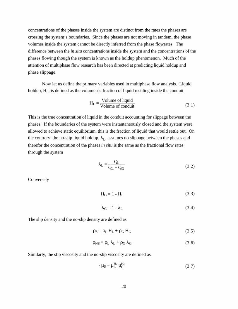
Now let us define the primary variables used in multiphase flow analysis. Liquid
holdup, HL, is defined as the volumetric fraction of liquid residing inside the conduit
HL = Volume of liquid
Volume of conduit (3.1)
This is the true concentration of liquid in the conduit accounting for slippage between the
phases. If the boundaries of the system were instantaneously closed and the system were
allowed to achieve static equilibrium, this is the fraction of liquid that would settle out. On
the contrary, the no-slip liquid holdup, λL, assumes no slippage between the phases and
therefor the concentration of the phases in situ is the same as the fractional flow rates
through the system
λL = QL
QL + QG (3.2)
Conversely
HG = 1 - HL (3.3)
λG = 1 - λL (3.4)
The slip density and the no-slip density are defined as
ρS = ρL HL + ρG HG (3.5)
ρNS = ρL λL + ρG λG (3.6)
Similarly, the slip viscosity and the no-slip viscosity are defined as
µS = µLHL µG
HG (3.7)
21
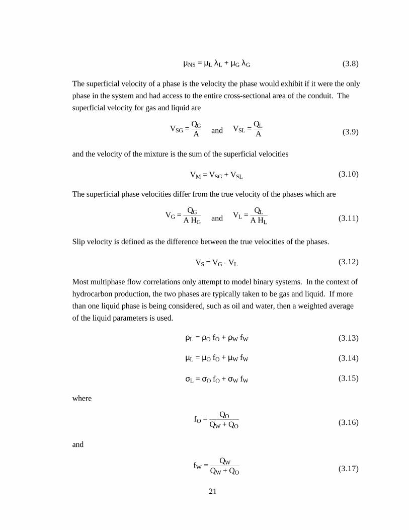
µNS = µL λL + µG λG (3.8)
The superficial velocity of a phase is the velocity the phase would exhibit if it were the only
phase in the system and had access to the entire cross-sectional area of the conduit. The
superficial velocity for gas and liquid are
VSG = QG
A and VSL =
QL
A (3.9)
and the velocity of the mixture is the sum of the superficial velocities
VM = VSG + VSL (3.10)
The superficial phase velocities differ from the true velocity of the phases which are
VG = QG
A HG and VL =
QL
A HL (3.11)
Slip velocity is defined as the difference between the true velocities of the phases.
VS = VG - VL (3.12)
Most multiphase flow correlations only attempt to model binary systems. In the context of
hydrocarbon production, the two phases are typically taken to be gas and liquid. If more
than one liquid phase is being considered, such as oil and water, then a weighted average
of the liquid parameters is used.
ρL = ρO fO + ρW fW (3.13)
µL = µO fO + µW fW (3.14)
σL = σO fO + σW fW (3.15)
where
fO = QO
QW + QO (3.16)
and
fW = QW
QW + QO (3.17)
22
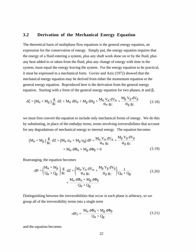
3.2 Derivation of the Mechanical Energy Equation
The theoretical basis of multiphase flow equations is the general energy equation, an
expression for the conservation of energy. Simply put, the energy equation requires that
the energy of a fluid entering a system, plus any shaft work done on or by the fluid, plus
any heat added to or taken from the fluid, plus any change of energy with time in the
system, must equal the energy leaving the system. For the energy equation to be practical,
it must be expressed in a mechanical form. Govier and Aziz (1972) showed that the
mechanical energy equation may be derived from either the momentum equation or the
general energy equation. Reproduced here is the derivation from the general energy
equation. Starting with a form of the general energy equation for two phases, α and β,
dζ = Mα + Mβ ggC
dZ + Mα dHα + Mβ dHβ + Mα Vα dVααα gC
+ Mβ Vβ dVβ
αβ gC(3.18)
we must first convert the equation to include only mechanical forms of energy. We do this
by substituting, in place of the enthalpy terms, terms involving irreversibilities that account
for any degradations of mechanical energy to internal energy. The equation becomes
Mα + Mβ ggC
dZ + Mα υα + Mβ υβ dP + Mα Vα dVααα gC
+ Mβ Vβ dVβ
αβ gC
+ Mα dΦα + Mβ dΦβ = 0 (3.19)
Rearranging, the equation becomes
-dP = Mα + Mβ
Qα + Qβ
ggC
dZ + Mα Vα dVααα gC
+ Mβ Vβ dVβ
αβ gC 1Qα + Qβ
+ Mα dΦα + Mβ dΦβ
Qα + Qβ
(3.20)
Distinguishing between the irreversibilities that occur in each phase is arbitrary, so we
group all of the irreversibility terms into a single term
-dPF = Mα dΦα + Mβ dΦβ
Qα + Qβ(3.21)
and the equation becomes
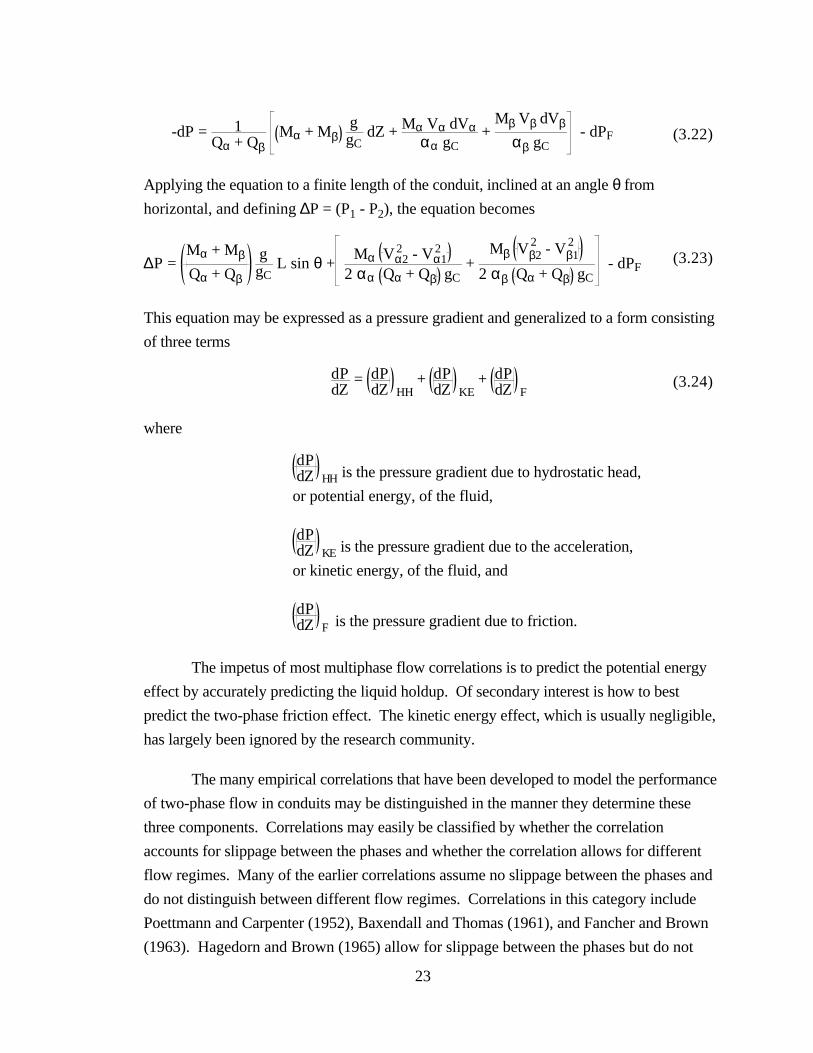
23
-dP = 1Qα + Qβ
Mα + Mβ ggC
dZ + Mα Vα dVααα gC
+ Mβ Vβ dVβ
αβ gC - dPF (3.22)
Applying the equation to a finite length of the conduit, inclined at an angle θ from
horizontal, and defining ∆P = (P1 - P2), the equation becomes
∆P = Mα + Mβ
Qα + Qβ ggC
L sin θ + Mα Vα2
2 - Vα12
2 αα Qα + Qβ gC +
Mβ Vβ22 - Vβ1
2
2 αβ Qα + Qβ gC - dPF
(3.23)
This equation may be expressed as a pressure gradient and generalized to a form consisting
of three terms
dPdZ
= dPdZ HH
+ dPdZ KE
+ dPdZ F
(3.24)
where
dPdZ HH is the pressure gradient due to hydrostatic head,
or potential energy, of the fluid,
dPdZ KE is the pressure gradient due to the acceleration,
or kinetic energy, of the fluid, and
dPdZ F is the pressure gradient due to friction.
The impetus of most multiphase flow correlations is to predict the potential energy
effect by accurately predicting the liquid holdup. Of secondary interest is how to best
predict the two-phase friction effect. The kinetic energy effect, which is usually negligible,
has largely been ignored by the research community.
The many empirical correlations that have been developed to model the performance
of two-phase flow in conduits may be distinguished in the manner they determine these
three components. Correlations may easily be classified by whether the correlation
accounts for slippage between the phases and whether the correlation allows for different
flow regimes. Many of the earlier correlations assume no slippage between the phases and
do not distinguish between different flow regimes. Correlations in this category include
Poettmann and Carpenter (1952), Baxendall and Thomas (1961), and Fancher and Brown
(1963). Hagedorn and Brown (1965) allow for slippage between the phases but do not
24
account for different flow regimes. The more recent correlations of Duns & Ros (1963),
Orkiszewski (1967), Aziz et al. (1972), and Beggs & Brill (1973) account for slippage
between the phases and provide different algorithms to model different flow regimes.
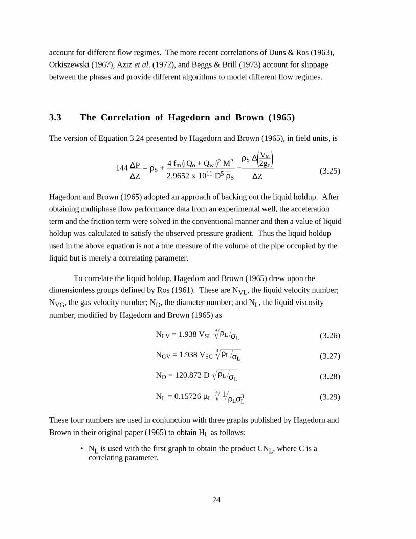
3.3 The Correlation of Hagedorn and Brown (1965)
The version of Equation 3.24 presented by Hagedorn and Brown (1965), in field units, is
144 ∆P∆Z
= ρS + 4 fm Qo + Qw 2 M2
2.9652 x 10¹¹ D5 ρS
+ρS ∆ VM
2gc
∆Z (3.25)
Hagedorn and Brown (1965) adopted an approach of backing out the liquid holdup. After
obtaining multiphase flow performance data from an experimental well, the acceleration
term and the friction term were solved in the conventional manner and then a value of liquid
holdup was calculated to satisfy the observed pressure gradient. Thus the liquid holdup
used in the above equation is not a true measure of the volume of the pipe occupied by the
liquid but is merely a correlating parameter.
To correlate the liquid holdup, Hagedorn and Brown (1965) drew upon the
dimensionless groups defined by Ros (1961). These are NVL, the liquid velocity number;
NVG, the gas velocity number; ND, the diameter number; and NL, the liquid viscosity
number, modified by Hagedorn and Brown (1965) as
NLV = 1.938 VSL ρL σL
4
(3.26)
NGV = 1.938 VSG ρL σL
4
(3.27)
ND = 120.872 D ρL σL (3.28)
NL = 0.15726 µL 1 ρLσL3
4
(3.29)
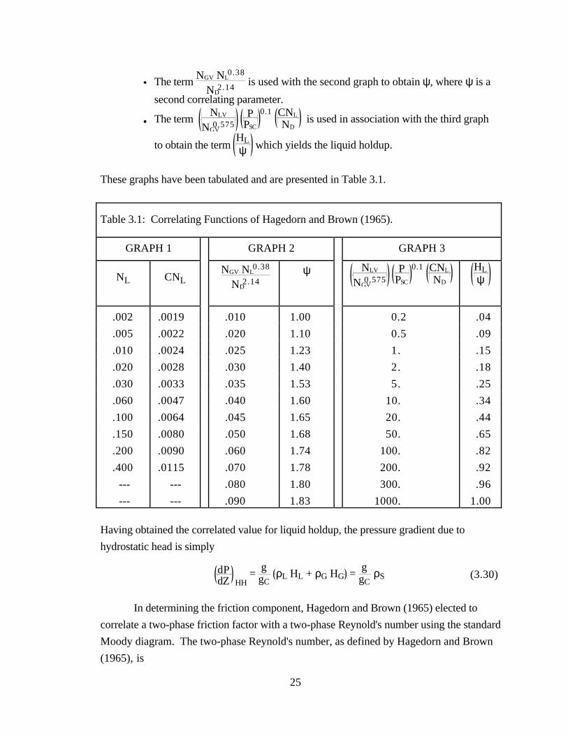
These four numbers are used in conjunction with three graphs published by Hagedorn and
Brown in their original paper (1965) to obtain HL as follows:
• NL is used with the first graph to obtain the product CNL, where C is acorrelating parameter.
25
• The term NGV NL
0.38
ND2.14 is used with the second graph to obtain ψ, where ψ is a
second correlating parameter.
• The term NLV
NGV0.575
PPSC
0.1 CNL
ND is used in association with the third graph
to obtain the term
HLψ
which yields the liquid holdup.
These graphs have been tabulated and are presented in Table 3.1.
Table 3.1: Correlating Functions of Hagedorn and Brown (1965).
GRAPH 1 GRAPH 2 GRAPH 3
NL CNL NGV NL
0.38
ND2.14
ψ NLV
NGV0.575
PPSC
0.1 CNL
ND HL
ψ
.002 .0019 .010 1.00 0.2 .04
.005 .0022 .020 1.10 0.5 .09
.010 .0024 .025 1.23 1. .15
.020 .0028 .030 1.40 2. .18
.030 .0033 .035 1.53 5. .25
.060 .0047 .040 1.60 10. .34
.100 .0064 .045 1.65 20. .44
.150 .0080 .050 1.68 50. .65
.200 .0090 .060 1.74 100. .82
.400 .0115 .070 1.78 200. .92
--- --- .080 1.80 300. .96
--- --- .090 1.83 1000. 1.00
Having obtained the correlated value for liquid holdup, the pressure gradient due to
hydrostatic head is simply
dPdZ HH
= ggC
ρL HL + ρG HG = ggC
ρS (3.30)
In determining the friction component, Hagedorn and Brown (1965) elected to
correlate a two-phase friction factor with a two-phase Reynold's number using the standard
Moody diagram. The two-phase Reynold's number, as defined by Hagedorn and Brown
(1965), is
26
ReHB = ρNS VM D
µS(3.31)
Having obtained the two-phase friction factor from a Moody diagram using the two-phase
Reynold’s number, the friction component of the total pressure gradient is given by
dPdZ F
= fM ρNS
2 VM2
2 gC ρSD(3.32)
We can account for the acceleration effects of the kinetic energy component by
defining EK as
EK = VM VSG ρNS
gC P (3.33)
The total pressure gradient is then given by
dPdZ
=
dPdZ HH
+ dPdZ F
1 - EK
(3.34)
Treating the acceleration component in this fashion requires caution: as the value of
EK approaches one, the total pressure gradient becomes indeterminant. This is physically
analogous to sonic or choked flow and is common for high gas velocities at low pressures.
Since numerical instabilities arise as you begin to approach one, the value of EK is typically
constrained below a certain ceiling value. In the model developed for this report, EK is not
allowed to exceed a conservative value of 0.6.
Many people employ a modified version of the Hagedorn and Brown (1965)
correlation, the modification being that the Griffith and Wallis (1961) method is used for
the bubble flow regime. The Griffith and Wallis (1961) modification is made if
VSGVM
< LB (3.35)
where
LB = 1.071 - 0.2218 VM
2
D ; LB ≥ 0.13 (3.36)
If the bubble flow regime is indicated, then the liquid holdup for bubble flow, as
determined by Griffith and Wallis (1961), is given by the expression
27
HL = 1 - 12
1 + VMVS
- 1 + VMVS
2 - 4 VSG
VS(3.37)
where the slip velocity, VS, is assumed to be constant at 0.8 ft/sec. The density component
of the total pressure gradient is determined from the expression
dPdZ HH
= ggC
ρs = ggC
ρL HL + ρG HG (3.38)
The friction component for the bubble flow region is based solely on the liquid phase and is
given by
dPdZ F
= fM ρL VSL
HL
2
2 gC D (3.39)
where the Moody friction factor is based on the Reynold’s number of the liquid
Re = ρL VSL D
HL µL(3.40)
The acceleration component was considered to be negligible in the bubble flow regime.
Therefore, the pressure gradient in the bubble flow regime is given by
dPdZ BUB
= dPdZ HH
+ dPdZ F
(3.41)
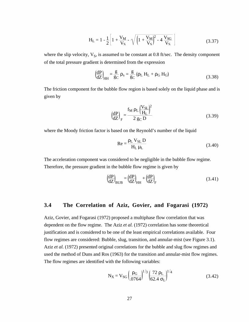
3.4 The Correlation of Aziz, Govier, and Fogarasi (1972)
Aziz, Govier, and Fogarasi (1972) proposed a multiphase flow correlation that was
dependent on the flow regime. The Aziz et al. (1972) correlation has some theoretical
justification and is considered to be one of the least empirical correlations available. Four
flow regimes are considered: Bubble, slug, transition, and annular-mist (see Figure 3.1).
Aziz et al. (1972) presented original correlations for the bubble and slug flow regimes and
used the method of Duns and Ros (1963) for the transition and annular-mist flow regimes.
The flow regimes are identified with the following variables:
NX = VSG ρG
.0764
1 3
72 ρL
62.4 σL
1 4(3.42)

28
NY = VSL 72 ρL
62.4 σL
1 4(3.43)
Bubble Slug Transition Mist
Figure 3.1: Flow Regimes of Aziz, Govier, and Fogarasi (1972).
NX and NY give the location within the flow map while the boundaries of the flow regimes
are given by
B12 = 0.51 100 NY0.172 (3.44)
B23 = 8.6 + 3.8 NY (3.45)
B34 = 70 100 NY-0.152 (3.46)
The flow regimes may be identified as follows:
Bubble Flow: NX < B12 (3.47)
Slug Flow: B12 ≤ NX < B23 (3.48)
Transition Flow: B23 ≤ NX < B34 ; NY < 4 (3.49)
Annular-Mist: B34 ≤ NX (3.50)
The Aziz et al. (1972) flow map is presented in Figure 3.2.

29
A paper by Hazim and Nimat (1989) proposed that the performance of the Aziz et
al. (1972) correlation could be improved by using other flow-pattern maps instead of the
map proposed by Aziz et al. (1972). For their specific data set, best performance was
attained when the Aziz et al. (1972) correlation was used in conjunction with the Duns and
Ros (1963) flow-pattern map.
Bubble
Slug
Transition
Annular-MistB23 B
34
B12
0.1 1.0 10. 100. 1000.
.01
0.1
1.0
10.
Ny
Nx
Figure 3.2: Flow-Pattern Map Proposed by Aziz, Govier, and Fogarasi (1972).
3.4.1 Bubble Flow Regime
To obtain the pressure gradient due to fluid density in the bubble flow regime, Aziz et al.
(1972) proposed to define the liquid holdup as
HL = 1 - VSGVBF (3.51)
where the absolute bubble rise velocity is
VBF = 1.2 VM + VBS (3.52)
and the bubble rise velocity is
VBS = 1.41 σL g ρL - ρG
ρL2
1 4(3.53)
30
The hydrostatic head component of the total pressure gradient is then
dPdZ HH
= ggC
ρL HL + ρG HG = ggC
ρS (3.54)
To determine the friction component, they proposed to use
dPdZ F
= fM ρS VM
2
2 gC D(3.55)
where the Moody friction factor is obtained using a Reynold’s number of
Re = ρL VM D
µL(3.56)
The acceleration component was considered to be negligible in the bubble flow regime.
Therefore, the total pressure gradient for the bubble flow regime is given by
dPdZ BUB
= dPdZ HH
+ dPdZ F
(3.57)
3.4.2 Slug Flow Regime
The density component in the slug flow regime uses the same definition for liquid holdup
and VBF employed in the bubble flow regime. However, VBS is defined as
VBS = C g D ρL - ρG
ρL
1 2(3.58)
where
C = 0.345 1 - exp -0.029 NV 1 - exp 3.37 - NEm (3.59)
NE = g D ρL - ρG
σL(3.60)
NV = g D3 ρL ρL - ρG
1 2
µL
(3.61)
where m in Equation 3.59 is evaluated as follows:
NV m
31
NV ≤ 18 25 (3.62)
18 < NV < 250 69 NV-0.35
(3.63)
250 ≤ NV 10 (3.64)
Having obtained the liquid holdup, the hydrostatic head component of the total pressure
gradient is
dPdZ HH
= ggC
ρL HL + ρG HG = ggC
ρS (3.65)
The friction component in slug flow is evaluated as
dPdZ F
= fM ρL HL VM
2
2 gC D(3.66)
where the Moody friction is obtained using a Reynold’s number of
Re = ρL VM D
µL(3.67)
As in the bubble flow regime, the acceleration component was considered to be negligible
in the slug flow regime. Therefore, the total pressure gradient for the slug flow regime is
given by
dPdZ SLUG
= dPdZ HH
+ dPdZ F
(3.68)
3.4.3 Transition Flow Regime
The transition flow region is, as the name indicates, a region of transition between the slug
flow region and the annular-mist flow region. When flow occurs within the transition
region, the pressure gradient is obtained by performing a linear interpolation between the
slug and annular-mist regions, as suggested by Duns and Ros (1963). The interpolation is
performed as follows:
dPdZ TRANS
= N3 - NXN3 - N2
dPdZ SLUG
+ NX - N2N3 - N2
dPdZ MIST (3.69)
32
3.4.4 Annular-Mist Flow Regime
For modeling the annular-mist flow regime, Aziz et al. (1972) used the procedure
developed by Duns and Ros (1963). Duns and Ros assumed that the high gas velocity of
the annular-mist region would allow no slippage to occur between the phases. The mixture
density used to calculate the density component is, therefore, the no-slip density, ρNS. The
expression for the density component is
dPdZ HH
= ggC
ρNS = ggC
ρL λL + ρG λG (3.70)
The friction component for the annular-mist region is based solely on the gas phase
and is given by
dPdZ F
= fM ρG VSG
2
2 gC D(3.71)
where the Moody friction factor is based on the Reynold’s number of the gas
Re = ρG VSG D
µG(3.72)
Duns and Ros (1963) gave special treatment to the manner that the relative
roughness was determined. They discovered that the pipe roughness was altered by the
thin layer of liquid on the wall of the pipe. Two variables are used to characterize this
effect. The first is a form of the Weber number
NWE = ρG VSG
2 εσL
(3.73)
and the second is dimensionless number based on liquid viscosity
Nµ = µL
ρL σL ε (3.74)
Duns and Ros (1963) proposed the following relationship to model the relative roughness:
NWE Nµ ≤ 0.005 εD
= 0.0749 σL
ρG VSG2 D (3.75)
33
NWE Nµ > 0.005 εD
= 0.3713 σL
ρG VSG2 D
NWE Nµ0.302
(3.76)
The value of the relative roughness is constrained to be no less than the actual relative
roughness of the pipe and no more than 0.5.
For values of relative roughness greater than 0.05, the limits of the Moody diagram
are approached. Duns and Ros (1963) proposed the following relation for the moody
friction factor for values of relative roughness greater than 0.05:
fM = 4 1
4 log 0.27 εD
2 + 0.067 ε
D1.73
(3.77)
We can account for the acceleration component by defining EK as
EK = VM VSG ρNS
gC P (3.78)
The total pressure gradient is then given by
dPdZ MIST
=
dPdZ HH
+ dPdZ F
1 - EK
(3.79)
As mentioned earlier, treating the kinetic energy term in this fashion requires care as the
term will become indeterminant as EK approaches one.
3.5 The Correlation of Orkiszewski (1967):
The work of Orkiszewski (1967) is a composite product: after testing the available
correlations for their accuracy, he selected the flow correlations he considered to be the
most accurate. These include the Griffith and Wallis (1961) method for bubble flow, the
Duns and Ros (1963) method for annular-mist flow and transition flow, and a method he
proposed for slug flow. The Griffith and Wallis (1961) method was previously discussed
with the Hagedorn and Brown (1965) correlation and the Duns and Ros (1963) method
was previously discussed with the Aziz et al. (1972) correlation. Discussion of these
methods will not be repeated here.

34
Orkiszewski's contribution was an original correlation to model slug flow. The
flow map of Orkiszewski (1967) is partitioned by the boundaries of
LB = 1.071 - 0.2218 VM
2
D ; LB ≥ 0.13 (3.80)
LS = 50 + 36 NLV (3.81)
LM = 75 + 84 NLV0.75 (3.82)
where the dimensionless numbers NLV and NGV, as proposed by Ros (1961), are
NLV = VSL ρL
g σ
4
(3.83)
NGV = VSG ρL
g σ
4
(3.84)
The flow regimes are identified by the following rules:
BubbleVSGVM
< LB
SlugVSGVM
> LB and NGV < LS
Transition LS < NGV < LM
Annular-Mist LM < NGV
The flow-pattern map suggested by Orkiszewski (1967) is shown in Figure 3.3.

35
BubbleGriffith & Wallis
SlugOrkeszewski
TransitionDuns & Ros Mist
Duns & Ros
0.1 10. 100. 1000.
0.1
1.0
10.
100.
NLV
NGV
1.0
VSG / VM = LBNGV = 36 NLV + 50 NGV = 84 NLV^0.75 + 75
Figure 3.3: Flow-Pattern Map Proposed by Orkiszewski (1967).
To model the slug flow regime, Orkiszewski (1967) defined two-phase density as
ρS = ρL VSL + VB + ρG VSG
VM + VB + ρL δ (3.85)
Two different Reynold’s numbers are required to find VB
NREB = ρL VB D
µL(3.86)
NREL = ρL VM D
µL(3.87)
The procedure to find VB is iterative:
1. Estimate VB. Orkiszewski (1967) recommends VB = 0.5 g D.
2. Calculate NREB using the value of VB from step 1.
3. Calculate VB according to the following rule set.
4. Repeat until convergence is achieved.

36
The rule-set to evaluate VB is
NREB ≤ 3000 VB = 0.546 + 8.74x10⁻⁶ NREL g D (3.88)
3000 < NREB < 8000ξ = 0.251 + 8.7x10⁻⁶ NREL g D
VB = 12
ξ + ξ2 +
13.59 µL
ρL D(3.89)
8000 ≤ NREBVB = 0.35 + 8.74x10⁻⁶ NREL g D (3.90)
The variable δ in the two-phase density expression is given by
WOR VMδ
> 3 < 10 0.013 log µL
D1.38 - 0.681 + 0.232 log VM - 0.428 log D
(3.91)
> 3 > 10 0.045 log µL
D0.799 - 0.709 - 0.162 log VM - 0.888 log D
(3.92)
< 3 < 10 0.0127 log µL + 1
D1.415 - 0.284 + 0.167 log VM - 0.113 log D
(3.93)
< 3 > 100.0274 log µL + 1
D1.371 + 0.161 + 0.569 log D
-log VM 0.01 log µL + 1
D1.571 + 0.397 + 0.63 log D
(3.94)
where the value of δ is constrained by
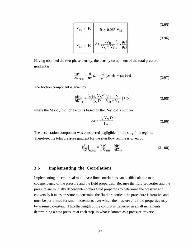
37
VM < 10 δ ≥ -0.065 VM
(3.95)
VM > 10 δ ≥ -VBVM + VB
1 - ρS
ρL
(3.96)
Having obtained the two-phase density, the density component of the total pressure
gradient is
dPdZ HH
= ggC
ρs = ggC
ρL HL + ρG HG (3.97)
The friction component is given by
dPdZ F
= fM ρL VM
2
2 gC DVSL + VBVM + VB
+ δ (3.98)
where the Moody friction factor is based on the Reynold’s number
Re = ρL VM D
µL(3.99)
The acceleration component was considered negligible for the slug flow regime.
Therefore, the total pressure gradient for the slug flow regime is given by
dPdZ SLUG
= dPdZ HH
+ dPdZ F
(3.100)
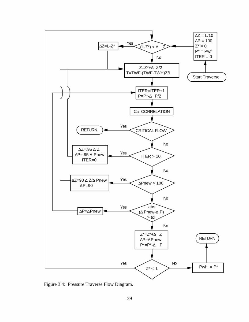
3.6 Implementing the Correlations
Implementing the empirical multiphase flow correlations can be difficult due to the
codependency of the pressure and the fluid properties. Because the fluid properties and the
pressure are mutually dependent--it takes fluid properties to determine the pressure and
conversely it takes pressure to determine the fluid properties--the procedure is iterative and
must be performed for small increments over which the pressure and fluid properties may
be assumed constant. Thus the length of the conduit is traversed in small increments,
determining a new pressure at each step, in what is known as a pressure traverse.
38
Although a pressure traverse may be performed by iterating on either length or on
pressure, iterating on pressure is the preferred method. By iterating on pressure, the sum
of the length intervals can be set to equal the length of the conduit and no interpolation is
required in the final step. Moreover, the scheme of iterating on length can have numerical
difficulties associated with downward flow due to the friction component and the density
component working against each other. The general procedure of performing the pressure
traverse is detailed in Figure 3.4.
Gregory et al. (1980) demonstrated that the pressure traverse is direction
dependent. They concluded that significantly higher accuracy is achieved when the
pressure traverse proceeds from the high pressure region (bottomhole) to the low pressure
region (wellhead).
39
Start Traverse
∆Z = L/10∆P = 100Z* = 0P* = PwfITER = 0
(L-Z*) < ∆ Z∆Z=L-Z*
Z=Z*+∆ Z/2T=TWF-(TWF-TWH)Z/L
ITER=ITER+1P=P*-∆ P/2
Call CORRELATION
CRITICAL FLOW
ITER > 10
∆Pnew > 100
abs(∆ Pnew-∆ P) > tol
Z*=Z*+∆ Z∆P=∆PnewP*=P*-∆ P
Z* < L Pwh = P*
RETURN
RETURN
∆Z=.95 ∆ Z∆P=.95 ∆ Pnew ITER=0
∆Z=90 ∆ Z/∆ Pnew ∆P=90
∆P=∆Pnew
Yes
No
Yes
No
Yes
No
Yes
No
Yes
No
NoYes
Figure 3.4: Pressure Traverse Flow Diagram.
41
FLOWP1
P2
WELLHEAD
POSITIVEFLOWBEAN
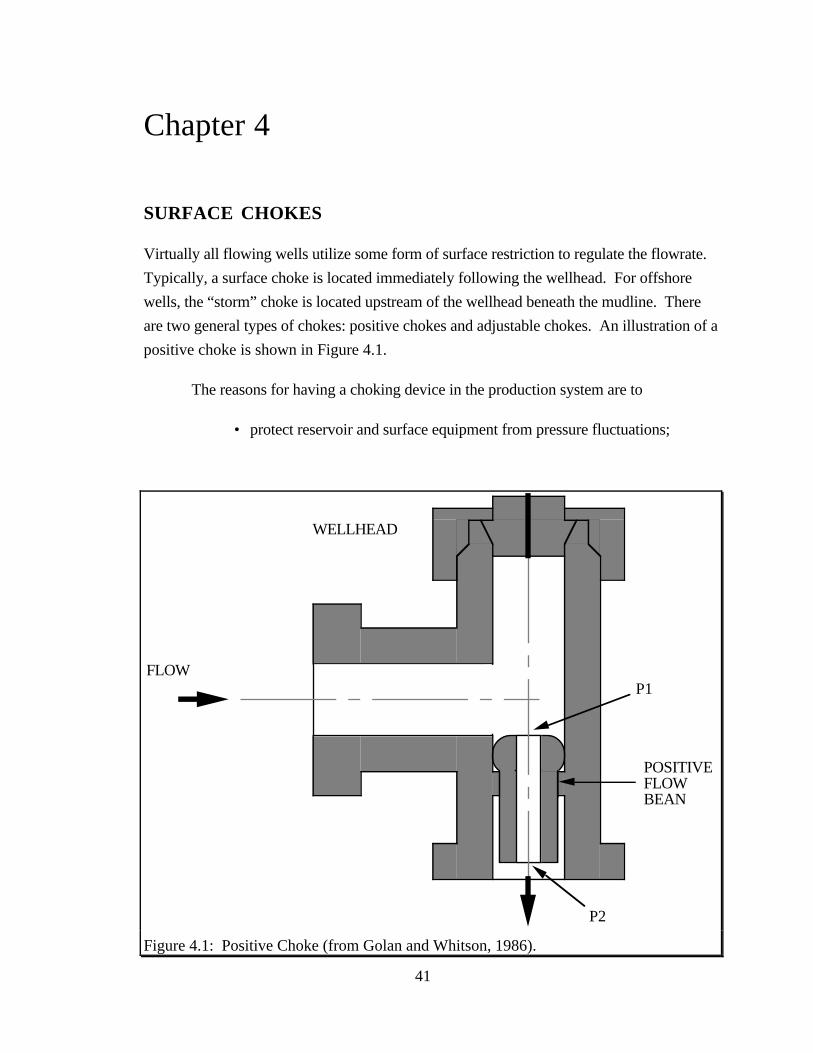
Figure 4.1: Positive Choke (from Golan and Whitson, 1986).
Chapter 4
SURFACE CHOKES
Virtually all flowing wells utilize some form of surface restriction to regulate the flowrate.
Typically, a surface choke is located immediately following the wellhead. For offshore
wells, the “storm” choke is located upstream of the wellhead beneath the mudline. There
are two general types of chokes: positive chokes and adjustable chokes. An illustration of a
positive choke is shown in Figure 4.1.
The reasons for having a choking device in the production system are to
• protect reservoir and surface equipment from pressure fluctuations;
42
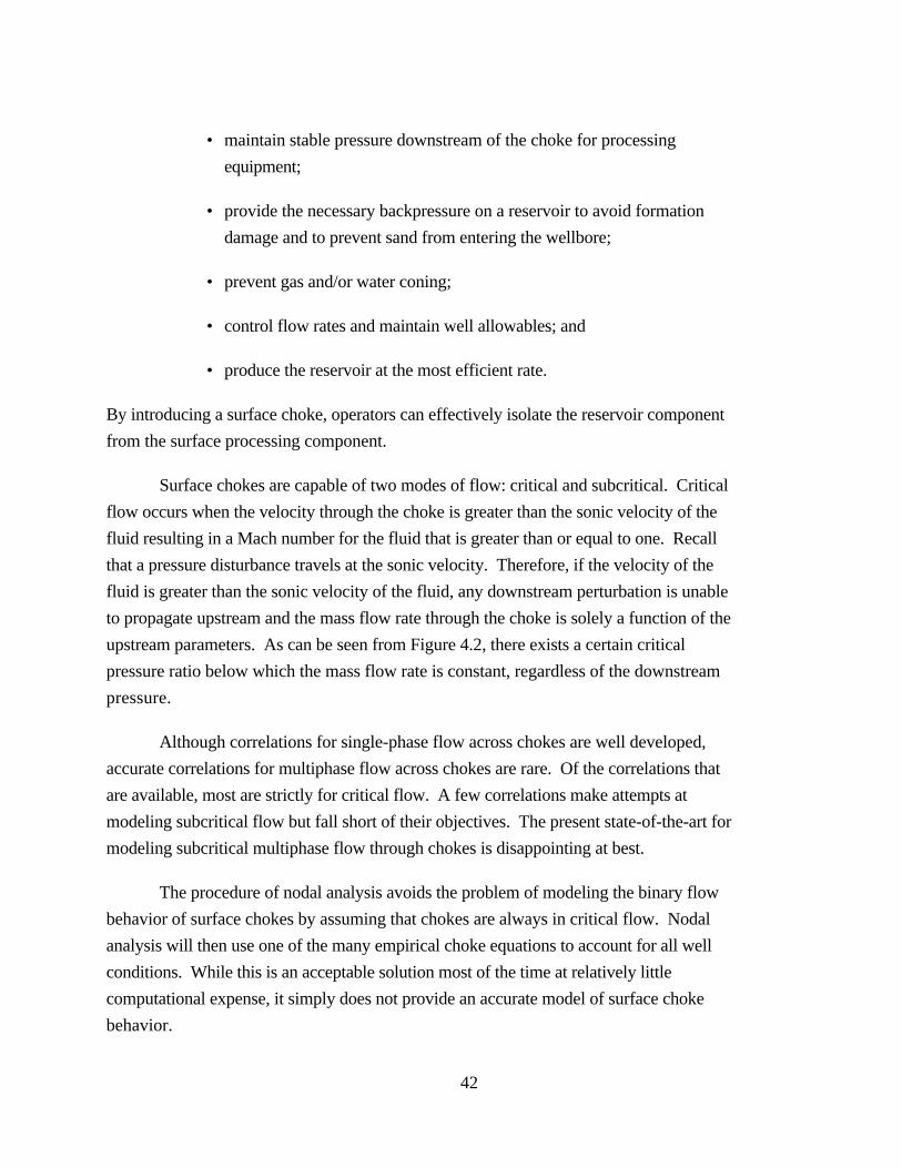
• maintain stable pressure downstream of the choke for processing
equipment;
• provide the necessary backpressure on a reservoir to avoid formation
damage and to prevent sand from entering the wellbore;
• prevent gas and/or water coning;
• control flow rates and maintain well allowables; and
• produce the reservoir at the most efficient rate.
By introducing a surface choke, operators can effectively isolate the reservoir component
from the surface processing component.
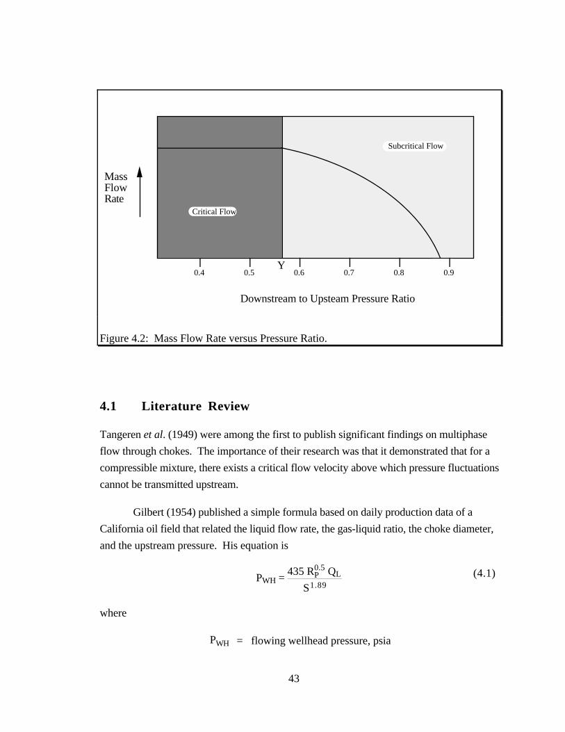
Surface chokes are capable of two modes of flow: critical and subcritical. Critical
flow occurs when the velocity through the choke is greater than the sonic velocity of the
fluid resulting in a Mach number for the fluid that is greater than or equal to one. Recall
that a pressure disturbance travels at the sonic velocity. Therefore, if the velocity of the
fluid is greater than the sonic velocity of the fluid, any downstream perturbation is unable
to propagate upstream and the mass flow rate through the choke is solely a function of the
upstream parameters. As can be seen from Figure 4.2, there exists a certain critical
pressure ratio below which the mass flow rate is constant, regardless of the downstream
pressure.
Although correlations for single-phase flow across chokes are well developed,
accurate correlations for multiphase flow across chokes are rare. Of the correlations that
are available, most are strictly for critical flow. A few correlations make attempts at
modeling subcritical flow but fall short of their objectives. The present state-of-the-art for
modeling subcritical multiphase flow through chokes is disappointing at best.
The procedure of nodal analysis avoids the problem of modeling the binary flow
behavior of surface chokes by assuming that chokes are always in critical flow. Nodal
analysis will then use one of the many empirical choke equations to account for all well
conditions. While this is an acceptable solution most of the time at relatively little
computational expense, it simply does not provide an accurate model of surface choke
behavior.
43
Downstream to Upsteam Pressure Ratio
MassFlowRate
Critical Flow
Subcritical Flow
0.4 0.5 0.6 0.7 0.8 0.9Y
Figure 4.2: Mass Flow Rate versus Pressure Ratio.
4.1 Literature Review
Tangeren et al. (1949) were among the first to publish significant findings on multiphase
flow through chokes. The importance of their research was that it demonstrated that for a
compressible mixture, there exists a critical flow velocity above which pressure fluctuations
cannot be transmitted upstream.
Gilbert (1954) published a simple formula based on daily production data of a
California oil field that related the liquid flow rate, the gas-liquid ratio, the choke diameter,
and the upstream pressure. His equation is
PWH = 435 RP
0.5 QL
S1.89(4.1)
where
PWH = flowing wellhead pressure, psia
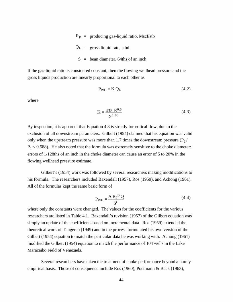
44
RP = producing gas-liquid ratio, Mscf/stb
QL = gross liquid rate, stbd
S = bean diameter, 64ths of an inch
If the gas-liquid ratio is considered constant, then the flowing wellhead pressure and the
gross liquids production are linearly proportional to each other as
PWH = K QL (4.2)
where
K = 435 R0.5
S1.89(4.3)
By inspection, it is apparent that Equation 4.3 is strictly for critical flow, due to the
exclusion of all downstream parameters. Gilbert (1954) claimed that his equation was valid
only when the upstream pressure was more than 1.7 times the downstream pressure (P2 /
P1 < 0.588). He also noted that the formula was extremely sensitive to the choke diameter:
errors of 1/128ths of an inch in the choke diameter can cause an error of 5 to 20% in the
flowing wellhead pressure estimate.
Gilbert’s (1954) work was followed by several researchers making modifications to
his formula. The researchers included Baxendall (1957), Ros (1959), and Achong (1961).
All of the formulas kept the same basic form of
PWH = A RP
B Q
SC(4.4)
where only the constants were changed. The values for the coefficients for the various
researchers are listed in Table 4.1. Baxendall’s revision (1957) of the Gilbert equation was
simply an update of the coefficients based on incremental data. Ros (1959) extended the
theoretical work of Tangeren (1949) and in the process formulated his own version of the
Gilbert (1954) equation to match the particular data he was working with. Achong (1961)
modified the Gilbert (1954) equation to match the performance of 104 wells in the Lake
Maracaibo Field of Venezuela.
Several researchers have taken the treatment of choke performance beyond a purely
empirical basis. Those of consequence include Ros (1960), Poetmann & Beck (1963),

45
Table 4.1: Empirical Coefficients for Two-Phase Critical Flow Correlations.
Correlation A B C
Gilbert (1954) 10.00 0.546 1.89
Baxendall (1957) 9.56 0.546 1.93
Ros (1959) 17.40 0.500 2.00
Achong (1961) 3.82 0.650 1.88
Omana et al. (1969), Fortunati (1972), Ashford & Pierce (1975), and Sachdeva et al.
(1986). It should be pointed out that only Fortunati (1972), Ashford & Pierce (1975), and
Sachdeva et al. (1986) have attempted to model both critical and subcritical flow.
Ros (1960) extended the work of Tangeren (1949) to account for mist flow where
gas is the continuous phase. Ros (1960) demonstrated that accelerational effects dominate
choke behavior and that slippage effects are negligible. Poetmann & Beck (1963)
converted the Ros (1960) equation to field units and presented it as a series of nomographs.
Omana et al. (1969) conducted experiments with water and natural gas flowing
through restrictions. They performed a dimensional analysis that yielded eight
dimensionless groups to characterize the flow. A regression analysis produced an
empirical correlation based on five of these dimensionless groups. The Omana (1969)
correlation was never widely accepted because it was based on small diameters (4 to 14 /
64ths of an inch), low flow rates (800 bpd maximum), low pressure (400 to 1000 psig),
and the correlation was developed for a water-gas mixture as opposed to an oil-gas
mixture.
Fortunati (1972) demonstrated how to apply the findings of Guzhov and
Medviediev (1962) to model the performance of a surface choke. Guzhov and Medviediev
(1962) developed a curve relating the velocity of the mixture, VM, to the pressure ratio of
downstream pressure to upstream pressure, P2 / P1, where P1 was constant at 19.8 psia.
Fortunati (1972) showed how to correct the the mixture velocity for the actual downstream
pressure. Having the corrected velocity of the mixture, the determination of the liquid
46
flowrate is straightforward. Fortunati’s (1972) work was one of the first to be applicable
to both critical and subcritical flow.
Ashford & Pierce (1975) presented an analytic method to determine critical and
subcritical flow rates in subsurface safety valves. Their model was based on actual field
tests and included oil and water flow, as well as free gas and solution gas. They derived an
expression to predict the pressure ratio of downstream to upstream pressure, P2 / P1, at the
critical-subcritical flow boundary. They assumed that the derivative of mass flow rate to
the pressure ratio is zero at critical flow conditions. One of the shortcomings of the
Ashford & Pierce (1975) model is their definition of the downstream pressure. Ideally, P2
is the lowest pressure reached in the choke. In practice, this pressure cannot be easily
measured and without uncertainty.
4.2 The Sachdeva et al. (1986) Choke Model
One of the most recent treatments of the choke problem was performed by Sachdeva et al.
(1986). The premise of their work is the determination of the critical pressure ratio and is
an extension of the work of Ashford & Pierce (1975). In their 1986 paper, Sachdeva et al.
(1986) outline a procedure to determine the critical pressure ratio as well as the actual
pressure ratio.
Although the Sachdeva et al. (1986) model is, perhaps, the best method we
currently have at our disposal, it nevertheless is rife with limiting assumptions. Some of
these assumptions are
• the gas phase contracts isentropically but expands polytropically;
• flow is one-dimensional;
• phase velocities are equal at the throat (no slippage occurs between the
phases);
• the predominant influence on pressure is accelerational;
• the quality of the mixture is constant across the choke (no mass transfer
between the phases);
• the liquid phase is incompressible.
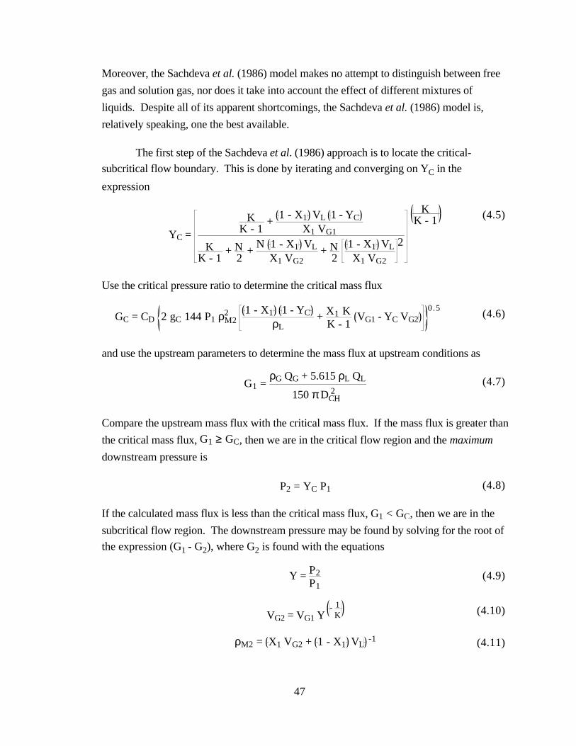
47
Moreover, the Sachdeva et al. (1986) model makes no attempt to distinguish between free
gas and solution gas, nor does it take into account the effect of different mixtures of
liquids. Despite all of its apparent shortcomings, the Sachdeva et al. (1986) model is,
relatively speaking, one the best available.
The first step of the Sachdeva et al. (1986) approach is to locate the critical-
subcritical flow boundary. This is done by iterating and converging on YC in the
expression
YC =
KK - 1
+ 1 - X1 VL 1 - YC
X1 VG1
KK - 1
+ N2
+ N 1 - X1 VL
X1 VG2 + N
2
1 - X1 VL
X1 VG2
2
KK - 1 (4.5)
Use the critical pressure ratio to determine the critical mass flux
GC = CD 2 gC 144 P1 ρM22
1 - X1 1 - YC
ρL + X1 K
K - 1 VG1 - YC VG2
0.5(4.6)
and use the upstream parameters to determine the mass flux at upstream conditions as
G1 = ρG QG + 5.615 ρL QL
150 π DCH2
(4.7)
Compare the upstream mass flux with the critical mass flux. If the mass flux is greater than
the critical mass flux, G1 ≥ GC, then we are in the critical flow region and the maximum
downstream pressure is
P2 = YC P1 (4.8)
If the calculated mass flux is less than the critical mass flux, G1 < GC, then we are in the
subcritical flow region. The downstream pressure may be found by solving for the root of
the expression (G1 - G2), where G2 is found with the equations
Y = P2P1
(4.9)
VG2 = VG1 Y- 1
K (4.10)
ρM2 = X1 VG2 + 1 - X1 VL-1 (4.11)
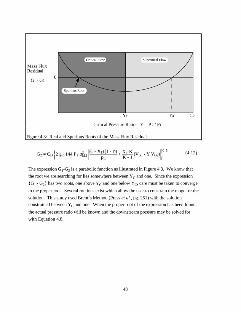
48
0
Yc Ya 1.0
Critical Pressure Ratio Y = P 2 / P1
Mass FluxResidual
G1 - G2
Spurious Root
Critical Flow Subcritical Flow
Figure 4.3: Real and Spurious Roots of the Mass Flux Residual.
G2 = CD 2 gC 144 P1 ρM22
1 - X1 1 - YρL
+ X1 KK - 1
VG1 - Y VG20.5
(4.12)
The expression G1-G2 is a parabolic function as illustrated in Figure 4.3. We know that
the root we are searching for lies somewhere between YC and one. Since the expression
G1 - G2 has two roots, one above YC and one below YC, care must be taken to converge
to the proper root. Several routines exist which allow the user to constrain the range for the
solution. This study used Brent’s Method (Press et al., pg. 251) with the solution
constrained between YC and one. When the proper root of the expression has been found,
the actual pressure ratio will be known and the downstream pressure may be solved for
with Equation 4.8.
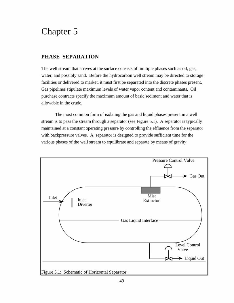
49
Gas Out
Liquid Out
Level Control Valve
Pressure Control Valve
Inlet InletDiverter
MistExtractor
Gas Liquid Interface
Figure 5.1: Schematic of Horizontal Separator.
Chapter 5
PHASE SEPARATION
The well stream that arrives at the surface consists of multiple phases such as oil, gas,
water, and possibly sand. Before the hydrocarbon well stream may be directed to storage
facilities or delivered to market, it must first be separated into the discrete phases present.
Gas pipelines stipulate maximum levels of water vapor content and contaminants. Oil
purchase contracts specify the maximum amount of basic sediment and water that is
allowable in the crude.
The most common form of isolating the gas and liquid phases present in a well
stream is to pass the stream through a separator (see Figure 5.1). A separator is typically
maintained at a constant operating pressure by controlling the effluence from the separator
with backpressure valves. A separator is designed to provide sufficient time for the
various phases of the well stream to equilibrate and separate by means of gravity

50
PC
PC
PC
Gas Out
Gas Out
Gas Out
Feed High PressureSeparator
Intermediate Pressure Separator
Low PressureSeparator
Stock Tank
1 psig
Figure 5.2: Stage Separation (from Arnold 1986).
segregation. The gas phase must exit from the top of the separator whereas the liquid
phase must exit from the bottom. The resulting gas may then be passed to a glycol
dehydrator for further removal of water vapor and contaminants before being delivered to a
pipeline. The liquid stream coming out of a separator may be passed through additional
separators operating at successively lower pressures before finally being delivered to the
stock tank (see Figure 5.2). Alternatively, the liquid stream may be passed through
gunbarrels, free water knock-outs, skim tanks, and heater treaters depending on the
specific treating requirements. Any solids present in the well stream are usually removed
by the force of gravity which may be augmented by hydrocyclones.
51
5.1 Optimization of Phase Separation
The optimization of phase separation practices is important because by varying the blend of
surface oil and gas produced per reservoir volume, an operator may markedly affect the
total value of the mix. The total value of the mix is affected by the fractional volumes
produced of each phase as well as the quality of each phase. The fractional volume of each
phase is important because traditionally the market has paid a significant premium for
hydrocarbons in the liquid phase. At times, the vapor phase was considered to be of no
economic value, prompting operators to flare the gas rather than attempt to find a market for
it. In addition to the gross volume produced of the oil and gas phases, the total value is
affected by the quality of the phases. A gas price is adjusted for the BTU content while the
price paid for crude varies with the API gravity of the oil.
An important concept in surface phase separation is that the fractional liquid
recovery will always be enhanced by adding more separators between the wellhead and the
stock tank. By increasing the number of separators, the liberation process between the
wellhead and the stock tank is essentially transformed from a flash liberation process to a
differential liberation process, thus improving the fractional liquid recovery. In a stage
separation process, the light hydrocarbons molecules that flash are removed at relatively
high pressure, keeping the partial pressure of the intermediate hydrocarbons lower at each
stage. As the number of stages approaches infinity, the lighter molecules are removed as
soon as they are formed and the partial pressure of the intermediate components is
maximized at each stage.
An equally important concept is that for a finite number of separators, there is an
optimal combination of discrete separator pressures that will maximize the fractional liquids
recovery. At the optimal combination of separator pressures, the API gravity of the crude
will be maximized and the gas-oil ratio will minimized (see Figure 5.3).
To mimic the behavior of surface facilities, this study elected to model the
performance of a two-stage separation process. A two-stage separation process involves
flashing the well stream initially at the separator operating conditions and then flashing the
resulting liquid stream at stock tank conditions. Assuming the temperatures of the two
stages to be constant and by setting the stock tank pressure to atmospheric pressure, the
separator pressure can be optimized to yield the most beneficial mix of oil and gas fractional
recoveries.
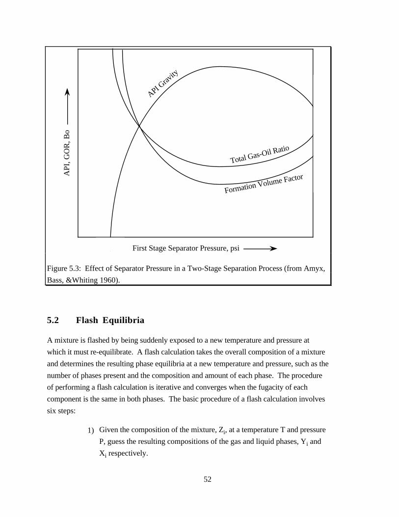
52
Total Gas-Oil Ratio
Formation Volume Factor
First Stage Separator Pressure, psi
API
, GO
R, B
o
API Grav
ity
Figure 5.3: Effect of Separator Pressure in a Two-Stage Separation Process (from Amyx,
Bass, &Whiting 1960).
5.2 Flash Equilibria
A mixture is flashed by being suddenly exposed to a new temperature and pressure at
which it must re-equilibrate. A flash calculation takes the overall composition of a mixture
and determines the resulting phase equilibria at a new temperature and pressure, such as the
number of phases present and the composition and amount of each phase. The procedure
of performing a flash calculation is iterative and converges when the fugacity of each
component is the same in both phases. The basic procedure of a flash calculation involves
six steps:
1) Given the composition of the mixture, Zi, at a temperature T and pressure
P, guess the resulting compositions of the gas and liquid phases, Yi and
Xi respectively.
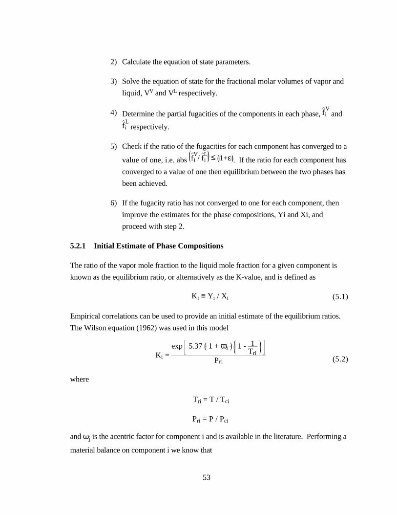
53
2) Calculate the equation of state parameters.
3) Solve the equation of state for the fractional molar volumes of vapor and
liquid, VV and VL respectively.
4) Determine the partial fugacities of the components in each phase, fiV and
fiL respectively.
5) Check if the ratio of the fugacities for each component has converged to a
value of one, i.e. abs fiV
/ fiL
≤ 1+ε . If the ratio for each component has
converged to a value of one then equilibrium between the two phases has
been achieved.
6) If the fugacity ratio has not converged to one for each component, then
improve the estimates for the phase compositions, Yi and Xi, and
proceed with step 2.
5.2.1 Initial Estimate of Phase Compositions
The ratio of the vapor mole fraction to the liquid mole fraction for a given component is
known as the equilibrium ratio, or alternatively as the K-value, and is defined as
Ki ≡ Yi / Xi (5.1)
Empirical correlations can be used to provide an initial estimate of the equilibrium ratios.
The Wilson equation (1962) was used in this model
Ki = exp 5.37 1 + ωi 1 - 1
Tri
Pri (5.2)
where
Tri = T / Tci
Pri = P / Pci
and ωi is the acentric factor for component i and is available in the literature. Performing a
material balance on component i we know that
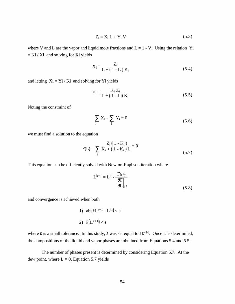
54
Zi = Xi L + Yi V (5.3)
where V and L are the vapor and liquid mole fractions and L = 1 - V. Using the relation Yi
= Ki / Xi and solving for Xi yields
Xi = ZiL + 1 - L Ki (5.4)
and letting Xi = Yi / Ki and solving for Yi yields
Yi = Ki ZiL + 1 - L Ki
(5.5)
Noting the constraint of
Xi - Yi = 0∑i
∑i
(5.6)
we must find a solution to the equation
F L = Zi 1 - Ki
Ki + 1 - Ki L = 0 ∑
i (5.7)
This equation can be efficiently solved with Newton-Raphson iteration where
Lk+1 = Lk - F Lk
∂F∂L Lk
(5.8)
and convergence is achieved when both
1)
2)
abs Lk+1 - Lk < ε
F Lk+1 < ε
where ε is a small tolerance. In this study, ε was set equal to 10-10. Once L is determined,
the compositions of the liquid and vapor phases are obtained from Equations 5.4 and 5.5.
The number of phases present is determined by considering Equation 5.7. At the
dew point, where L = 0, Equation 5.7 yields
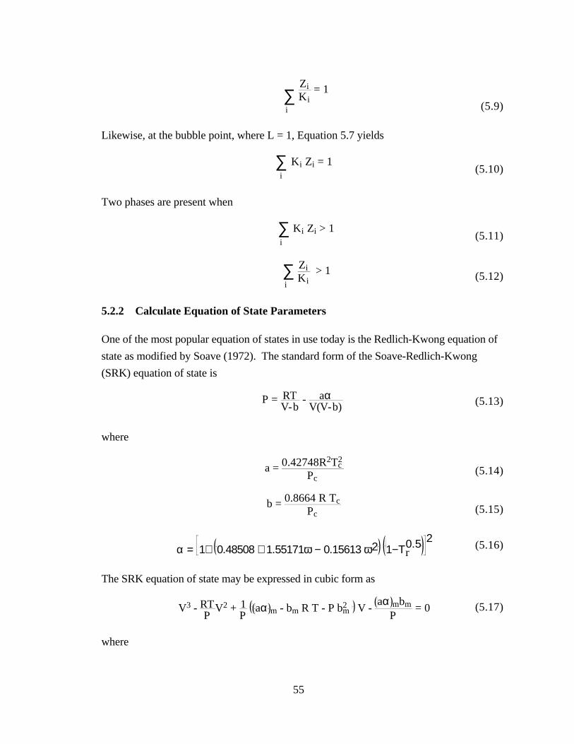
55
ZiKi
= 1 ∑i (5.9)
Likewise, at the bubble point, where L = 1, Equation 5.7 yields
Ki Zi∑i
= 1(5.10)
Two phases are present when
Ki Zi ∑i
> 1(5.11)
ZiKi
∑i
> 1 (5.12)
5.2.2 Calculate Equation of State Parameters
One of the most popular equation of states in use today is the Redlich-Kwong equation of
state as modified by Soave (1972). The standard form of the Soave-Redlich-Kwong
(SRK) equation of state is
P = RTV-b
- aαV(V-b)
(5.13)
where
a = 0.42748R2Tc2
Pc(5.14)
b = 0.8664 R TcPc (5.15)
α = 1+ 0.48508 + 1.55171ω − 0.15613 ω2 1−Τr0.5 2
(5.16)
The SRK equation of state may be expressed in cubic form as
V3 - RTP
V2 + 1P
aα m - bm R T - P bm2 V -
aα mbm
P = 0 (5.17)
where

56
aα m = YiYj aα i j∑j
∑i
(5.18)
bm = Yibi∑i
(5.19)
aα ij = 1 - Kij aα i aα j (5.20)
where Kij are the binary interaction parameters and may be obtained from Table 5.1.
Table 5.1: Binary Interaction Parameters for the Soave Equation
(Prausnitz 1986).H2S CO2 N2 CO
H2S --- 0.102 0.140 ---CO2 0.102 --- -0.022 -0.064N2 0.140 -0.022 --- 0.046
CO --- -0.064 0.046 ---
Methane 0.0850 0.0973 0.0319 0.03
Ethane 0.0829 0.1346 0.0388 0.00
n-Propane 0.0831 0.1018 0.0807 0.02
2-Methylpropane 0.0523 0.1358 0.1357 ---
n-Butane 0.0609 0.1474 0.1007 ---
2-Methylbutane --- 0.1262 --- ---
n-Pentane .0.697 0.1278 --- ---
n-Hexane --- --- 0.1444 ---
n-Heptane 0.0737 0.1136 --- ---
n-Octane --- --- --- 0.10
n-Nonane 0.0542 --- --- ---
n-Decane 0.0464 0.1377 0.1293 ---
Propylene --- 0.0914 --- ---
Cyclohexane --- 0.1087 --- ---
Isopropylcyclohexane 0.0562 --- --- 0.01
Benzene --- 0.0810 0.2131 ---
1,3,5-Trimethylbenzene 0.0282 --- --- ---
57
5.2.3 Solve Equation of State for VL and VV
The cubic form of the SRK equation of state must be solved for the liquid and vapor molar
volumes. An analytical solution was used to solve the cubic equation as follows. For a
cubic equation of the form
V3 + Α2 V2 + Α1 V + Α0 = 0 (5.21)
let
ψ = V + A2 / 3 (5.22)
Ω = 13
3 A1 - A2 (5.23)
δ = 127
2 A23 - 9 A2 A1 + 27 Ao (5.24)
µ = - δ2
- δ2
4 + Ω
3
27
1 3
(5.25)
λ = - δ2
+ δ2
4 + Ω
3
27
1 3
(5.26)
The roots of the cubic equation are
one real and two imaginary roots if δ2
4 + Ω
3
27 > 0
,
three real (two equal) roots if δ2
4 + Ω
3
27 = 0
,
or three real and nonequal roots if δ2
4 + Ω
3
27 < 0
.
For three real roots, let
cos θ = - δ
- 4 Ω27
(5.27)
Then
58
ψ1 = 2 cos θ3
- Ω3
(5.28)
ψ2 = 2 cos θ3
+ 2 π3
- Ω3
(5.29)
ψ3 = 2 cos θ3
+ 4 π3
- Ω3
(5.30)
5.2.4 Determine Partial Fugacities
For the Soave-Redlich-Kwong equation of state, the partial fugacity of component i is
given by
fi = P exp VV-bm
+ biV - bm
+ 2 Yi aij∑
R T bm ln V+bm
V
+ aα m bi
R T bm2
ln V + bV
- bmV + bm
- ln P VYi R T (5.31)
5.2.5 Convergence Check
A solution is found when the partial fugacity of each component is the same across all
phases.
fiV
fiL
= 1 for all i(5.32)
Since the algorithm is iterative, an exact solution is difficult if not impossible to achieve.
Instead, we must test if we are within some tolerance of this requirement. The convergence
criterion used in this study was whether the fugacity ratio for each component was within a
tolerance of ε of one:
abs fiV
/ fiL ≤ 1 + ε (5.33)
If the convergence criterion is met then the phase compositions and molar volumes are
known.

59
5.2.6 Modify the Vapor and Liquid Compositions
For the purposes of this study, a successive substitution scheme was used to estimate new
equilibrium ratios for successive iterations. The fugacity coefficient is defined as
φi
V = fi
V
Yi P (5.34)
φi
L = fi
L
Yi P (5.35)
It follows that
φi
L
φi
V = fi
L
fiV
YiXi
(5.36)
At equilibrium, the partial fugacities are equal. The equation simplifies to
φi
L
φi
V = Yi
Xi(5.37)
which is simply the definition of the equilibrium ratio. Therefore, we can used the fugacity
coefficients determined in the current unsuccessful iteration to estimate new K-values.
kik+1 = fi
L
fiV
kik
(5.38)
The new K-values are used to restart the procedure.
61
Chapter 6
NONLINEAR OPTIMIZATION
There are numerous problems for which people strive to find an optimal solution. These
problems might be minimizing the fuel consumption of an engine, maximizing the
efficiency of a process, or minimizing the volume occupied by a cluster of objects. It is
trivial to optimize a problem that depends on a single variable. It is when several variables
are optimized simultaneously that matters become complicated.
Mathematics can provide a powerful tool to optimize a problem, regardless of the
number of variables involved. Numerical optimization is the location of the extrema of a
mathematical model. The mathematical model, referred to as the objective function, accepts
multiple decision variables as input and returns a single value, the objective variable, as
output. Optimization strives to locate the minimum or maximum value of the objective
function.
Nonlinear optimization methods based on Newton’s technique locate the extrema by
approximating the objective function with a nonlinear quadratic model. Let the objective
function, F, be a nonlinear function of the vector of decision variables, x.
F = f x (6.1)
Newton’s method approximates the nonlinear objective function, F, with a quadratic
model, Q, which is also a function of the vector of decision variables, x.
Q x ≈ F x (6.2)
The quadratic approximation
Q x = cTx + 12
xT G x (6.3)
may be conceptualized, in two dimensions, as a bowl. If the matrix G is negative-definite,
the expression is bounded above and unbounded below (the bowl is upside-down) and will
therefore have a maximum (See Figure 6.1). Conversely, if the matrix G is positive
definite, the expression is bounded below and unbounded above (the bowl is right-side-up)
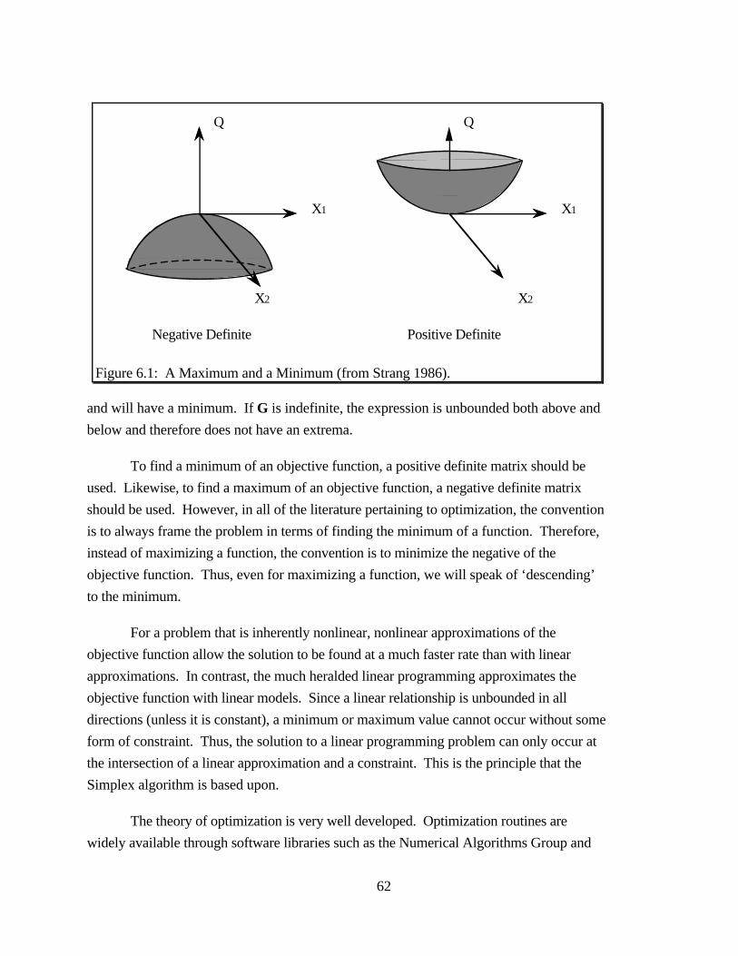
62
Q Q
X1 X1
X2X2
Negative Definite Positive Definite
Figure 6.1: A Maximum and a Minimum (from Strang 1986).
and will have a minimum. If G is indefinite, the expression is unbounded both above and
below and therefore does not have an extrema.
To find a minimum of an objective function, a positive definite matrix should be
used. Likewise, to find a maximum of an objective function, a negative definite matrix
should be used. However, in all of the literature pertaining to optimization, the convention
is to always frame the problem in terms of finding the minimum of a function. Therefore,
instead of maximizing a function, the convention is to minimize the negative of the
objective function. Thus, even for maximizing a function, we will speak of ‘descending’
to the minimum.
For a problem that is inherently nonlinear, nonlinear approximations of the
objective function allow the solution to be found at a much faster rate than with linear
approximations. In contrast, the much heralded linear programming approximates the
objective function with linear models. Since a linear relationship is unbounded in all
directions (unless it is constant), a minimum or maximum value cannot occur without some
form of constraint. Thus, the solution to a linear programming problem can only occur at
the intersection of a linear approximation and a constraint. This is the principle that the
Simplex algorithm is based upon.
The theory of optimization is very well developed. Optimization routines are
widely available through software libraries such as the Numerical Algorithms Group and
63
IMSL (1987). For a broad overview of numerical optimization techniques, see Gill,
Murray, & Wright (1981). For a more extensive treatment of numerical optimization
applied to petroleum engineering problems, see Barua (1989).
6.1 Newton’s Method
Newton’s Method is one of the most common techniques used in nonlinear optimization. It
is the standard against which all other algorithms are measured. If Newton’s Method is
provided with a good initial estimate of the solution, quadratic convergence is achieved.
Newton’s Method achieves this rate of convergence by approximating the objective
function with a quadratic model. The quadratic model is chosen so that, at a given point,
its first and second derivatives are identical to the first and second derivatives of the
objective function. Therefore, at the given point, the objective function and the quadratic
model are identical in value, slope, and curvature. The quadratic model is solved for the
stationary point where its gradient goes to zero. If the quadratic model is a good
approximation of the objective function, then the stationary point of the quadratic model
should be near a stationary point of the objective function. The stationary point of the
quadratic model is taken as the new estimate of the objective function’s stationary point and
the process is repeated until some form of convergence criteria is satisfied.
Taylor’s theorem provides the mathematical basis for Newton’s Method. Taylor’s
theorem states that if a function and its derivatives are known at a single point, then
approximations to the function can be made at all points in the immediate neighborhood of
the point. The Taylor series expansion of a general function F about x gives a simple
approximation to the function F in the immediate neighborhood of x as
F x+p = F x + g T p + 12
p T H p + O ||p||3 (6.4)
where x is the vector of variables,
x =
x1x2x3
xn
(6.5)

64
p is the vector of displacement from x,
p =
∆x1
∆x2
∆x3
∆xn
(6.6)
g is the gradient n-vector of x,
g =
∂F∂x1∂F∂x2∂F∂x3
∂F∂xn
(6.7)
and H is the Hessian matrix of x,
H =
∂2F
∂x1∂x1
∂2F
∂x1∂x2
∂2F
∂x1∂x3
∂2F
∂x1∂xn
∂2F
∂x2∂x1
∂2F
∂x2∂x2
∂2F
∂x2∂x3
∂2F
∂x2∂xn
∂2F
∂x3∂x1
∂2F
∂x3∂x2
∂2F
∂x3∂x3
∂2F
∂x3∂xn
∂2F
∂xn∂x1
∂2F
∂xn∂x2
∂2F
∂xn∂x3
∂2F
∂xn∂xn
(6.8)
Considering only the first and second order terms of the Taylor’s series expansion
(Equation 6.4) gives a quadratic approximation of the function F in the neighborhood of x
as
Q x+p = F x + g T p + 12
p T H p (6.9)
65
The minimum of a function can occur only where the gradient vector vanishes and the
gradient vector vanishes only at a stationary point. To find the stationary point of the
quadratic approximation, we take the gradient of Q
∂Q∂x
= g + H p (6.10)
and equate this to zero. The resulting equation
H p = - g (6.11)
can only be satisfied by a stationary point. To solve for the step-direction p that will lead to
the stationary point, the Hessian must be inverted
p = - H-1 g (6.12)
The step-direction p indicates the displacement from the point x that would give the
stationary point of the quadratic model. The Newton step is defined as the product (ρ p)
where ρ is the scalar step-length and p is the step-direction vector. We can update our
estimate of the point x by taking a Newton step
x ← x + ρ p (6.13)
Thus, the method takes a step of length ρ in the p direction. In unmodified Newton’s
Method, the length of the Newton step is implicitly taken as unity.
If the objective function is quadratic in form, then the quadratic approximation is
exact and Newton's Method will converge to the stationary point in a single iteration. In
the more likely event that the objective function is not quadratic in form, the higher-order
terms that were ignored in the Taylor series expansion will become negligible as Newton’s
Method begins to converge on the stationary point. As the higher-order terms go to zero,
the quadratic model will provide a very good approximation to the local surface and the
method will approach quadratic convergence.
A key insight to Newton’s Method can be obtained by investigating the eigensystem
of the Hessian matrix. By performing spectral decomposition of the Hessian
H = V Λ VT (6.14)
66
we obtain V, the matrix of eigenvectors, and Λ, the diagonal matrix of eigenvalues. Since
the Hessian is symmetric and V is unitary, the inverted Hessian is given as
H-1 = V Λ-1 VT (6.15)
Expressing the gradient as a linear combination of the eigenvectors,
g = V α (6.16)
the step-direction is given by
p = - H-1 g (6.12)
= - V Λ-1 VT V α (6.17)
= - V Λ-1 α (6.18)
= - v1
λ1
v2
λ2
v3
λ3
vn
λn
α (6.19)
Recall from linear algebra that an eigenvalue that is close to zero indicates that the function
is close to being singular and therefore will change very little along the corresponding
eigenvector. Equation 6.19 indicates that the smaller an eigenvalue is, the larger the step-
direction will be in the direction of the corresponding eigenvector. Therefore, Newton’s
Method will take the largest strides in the directions that the function is least sensitive.
While this feature is desirable with regard to convergence, it is extremely threatening to the
stability of the algorithm if left unchecked. Since Newton’s Method is only a quadratic
approximation to the local surface of the objective function, all steps should be somewhat
tentative.
The primary expense of Newton’s Method is not the matrix solution (Equation
6.12), but the evaluation of the derivatives required for the gradient and the Hessian. If
analytic expressions are unavailable for the derivatives, they must be evaluated using finite
difference approximations. For n decision variables, n2 + n
2 second partial derivatives are
necessary for the Hessian (recall that the Hessian is symmetric) and n first partial
derivatives are necessary for the gradient. If ei is the ith unit vector and hi is the finite
difference interval for the ith decision variable (see Figure 6.2), then the elements of the
gradient are given by the expression
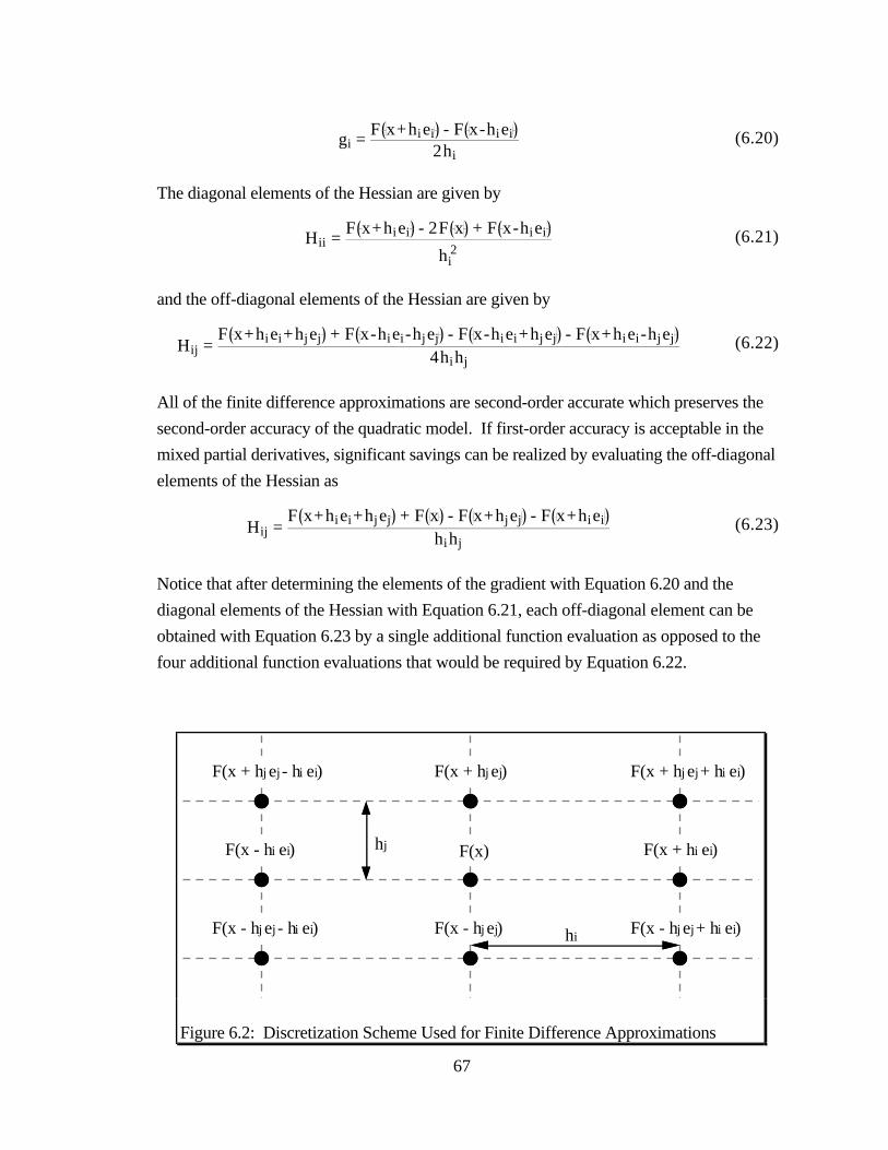
67
hj
hiF(x - hj ej) F(x - hj ej + hi ei)F(x - hj ej - hi ei)
F(x + hi ei)F(x)F(x - hi ei)
F(x + hj ej) F(x + hj ej + hi ei)F(x + hj ej - hi ei)
Figure 6.2: Discretization Scheme Used for Finite Difference Approximations
gi = F x+hiei - F x-hiei
2hi(6.20)
The diagonal elements of the Hessian are given by
Hii = F x+hiei - 2F x + F x-hiei
hi2
(6.21)
and the off-diagonal elements of the Hessian are given by
Hij = F x+hiei+hjej + F x-hiei-hjej - F x-hiei+hjej - F x+hiei-hjej
4hihj(6.22)
All of the finite difference approximations are second-order accurate which preserves the
second-order accuracy of the quadratic model. If first-order accuracy is acceptable in the
mixed partial derivatives, significant savings can be realized by evaluating the off-diagonal
elements of the Hessian as
Hij = F x+hiei+hjej + F x - F x+hjej - F x+hiei
hihj(6.23)
Notice that after determining the elements of the gradient with Equation 6.20 and the
diagonal elements of the Hessian with Equation 6.21, each off-diagonal element can be
obtained with Equation 6.23 by a single additional function evaluation as opposed to the
four additional function evaluations that would be required by Equation 6.22.
68
If used properly, Newton’s Method offers the fastest rate of convergence available.
However, this robust rate of convergence is achieved at the expense of the stability of the
algorithm. Some of the shortcomings of the method are
• A good initial starting point is required for convergence. A poor estimate
will result in divergence.
• If Newton’s Method does converge, it converges to the nearest stationary
point. No guarantee can be made that this is the desired stationary point.
It could be a local minimum, a maximum, or a saddlepoint.
• The Hessian matrix is subject to numerical instabilities during the matrix
solution.
• If the analytic derivatives are not available, the derivatives necessary to
construct the gradient and Hessian will have to be evaluated by very
costly finite difference approximations.
6.2 Modifications to Newton’s Method
In practice, the first modification made to Newton’s Method is to incorporate a one-
dimensional line search to obtain an improved step-length. Based largely on the credo of
“Look before you leap,” the line search is performed on the objective function in the
direction indicated by p. The line search locates, or approximates the location of, the
minimum in this single dimension. The distance to the minimum in this single dimension is
taken as the step-length ρ. This minimum is taken as the new estimate of x by taking a step
of length ρ in the p direction (Equation 6.13).
The next level of modifications made to Newton’s Method involve altering the
eigenvalues of the Hessian. The ideal modification will converge rapidly, with speed
approaching that of Newton’s Method, and will always be descending downhill towards
the minimum. A direction of descent is guaranteed if the Hessian is positive definite,
meaning that all of the eigenvalues are positive. Three methods are discussed that modify
Newton’s Method to produce a positive definite Hessian. These are the method of steepest
descent, the Marquardt (1963) modification, and the Greenstadt (1967) modification. The
method of steepest descent is included primarily for illustrative purposes and is not
recommended for practical usage.
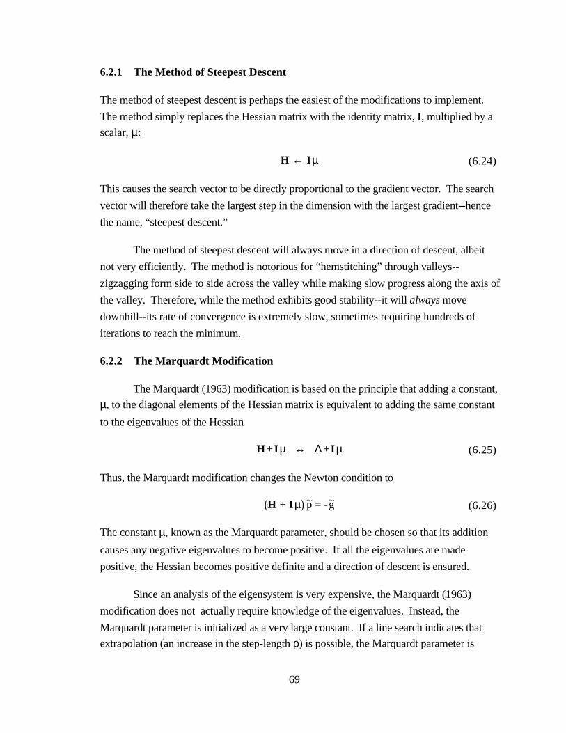
69
6.2.1 The Method of Steepest Descent
The method of steepest descent is perhaps the easiest of the modifications to implement.
The method simply replaces the Hessian matrix with the identity matrix, I, multiplied by a
scalar, µ:
H ← Iµ (6.24)
This causes the search vector to be directly proportional to the gradient vector. The search
vector will therefore take the largest step in the dimension with the largest gradient--hence
the name, “steepest descent.”
The method of steepest descent will always move in a direction of descent, albeit
not very efficiently. The method is notorious for “hemstitching” through valleys--
zigzagging form side to side across the valley while making slow progress along the axis of
the valley. Therefore, while the method exhibits good stability--it will always move
downhill--its rate of convergence is extremely slow, sometimes requiring hundreds of
iterations to reach the minimum.
6.2.2 The Marquardt Modification
The Marquardt (1963) modification is based on the principle that adding a constant,
µ, to the diagonal elements of the Hessian matrix is equivalent to adding the same constant
to the eigenvalues of the Hessian
H +Iµ ↔ Λ+Iµ (6.25)
Thus, the Marquardt modification changes the Newton condition to
H + Iµ p = -g (6.26)
The constant µ, known as the Marquardt parameter, should be chosen so that its addition
causes any negative eigenvalues to become positive. If all the eigenvalues are made
positive, the Hessian becomes positive definite and a direction of descent is ensured.
Since an analysis of the eigensystem is very expensive, the Marquardt (1963)
modification does not actually require knowledge of the eigenvalues. Instead, the
Marquardt parameter is initialized as a very large constant. If a line search indicates that
extrapolation (an increase in the step-length ρ) is possible, the Marquardt parameter is
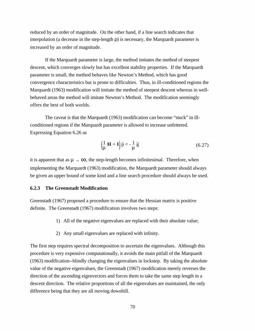
70
reduced by an order of magnitude. On the other hand, if a line search indicates that
interpolation (a decrease in the step-length ρ) is necessary, the Marquardt parameter is
increased by an order of magnitude.
If the Marquardt parameter is large, the method imitates the method of steepest
descent, which converges slowly but has excellent stability properties. If the Marquardt
parameter is small, the method behaves like Newton’s Method, which has good
convergence characteristics but is prone to difficulties. Thus, in ill-conditioned regions the
Marquardt (1963) modification will imitate the method of steepest descent whereas in well-
behaved areas the method will imitate Newton’s Method. The modification seemingly
offers the best of both worlds.
The caveat is that the Marquardt (1963) modification can become “stuck” in ill-
conditioned regions if the Marquardt parameter is allowed to increase unfettered.
Expressing Equation 6.26 as
1µ
H + I p = - 1µ
g (6.27)
it is apparent that as µ → ∞, the step-length becomes infinitesimal. Therefore, when
implementing the Marquardt (1963) modification, the Marquardt parameter should always
be given an upper bound of some kind and a line search procedure should always be used.
6.2.3 The Greenstadt Modification
Greenstadt (1967) proposed a procedure to ensure that the Hessian matrix is positive
definite. The Greenstadt (1967) modification involves two steps:
1) All of the negative eigenvalues are replaced with their absolute value;
2) Any small eigenvalues are replaced with infinity.
The first step requires spectral decomposition to ascertain the eigenvalues. Although this
procedure is very expensive computationally, it avoids the main pitfall of the Marquardt
(1963) modification--blindly changing the eigenvalues in lockstep. By taking the absolute
value of the negative eigenvalues, the Greenstadt (1967) modification merely reverses the
direction of the ascending eigenvectors and forces them to take the same step length in a
descent direction. The relative proportions of all the eigenvalues are maintained, the only
difference being that they are all moving downhill.
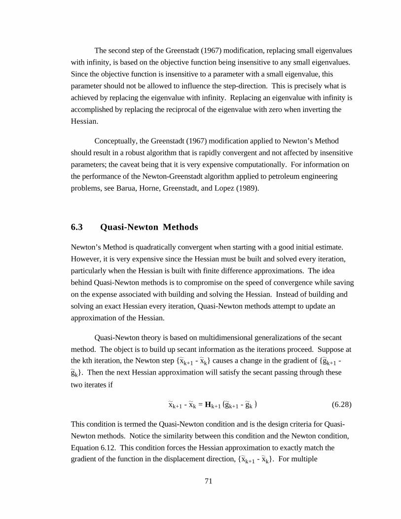
71
The second step of the Greenstadt (1967) modification, replacing small eigenvalues
with infinity, is based on the objective function being insensitive to any small eigenvalues.
Since the objective function is insensitive to a parameter with a small eigenvalue, this
parameter should not be allowed to influence the step-direction. This is precisely what is
achieved by replacing the eigenvalue with infinity. Replacing an eigenvalue with infinity is
accomplished by replacing the reciprocal of the eigenvalue with zero when inverting the
Hessian.
Conceptually, the Greenstadt (1967) modification applied to Newton’s Method
should result in a robust algorithm that is rapidly convergent and not affected by insensitive
parameters; the caveat being that it is very expensive computationally. For information on
the performance of the Newton-Greenstadt algorithm applied to petroleum engineering
problems, see Barua, Horne, Greenstadt, and Lopez (1989).
6.3 Quasi-Newton Methods
Newton’s Method is quadratically convergent when starting with a good initial estimate.
However, it is very expensive since the Hessian must be built and solved every iteration,
particularly when the Hessian is built with finite difference approximations. The idea
behind Quasi-Newton methods is to compromise on the speed of convergence while saving
on the expense associated with building and solving the Hessian. Instead of building and
solving an exact Hessian every iteration, Quasi-Newton methods attempt to update an
approximation of the Hessian.
Quasi-Newton theory is based on multidimensional generalizations of the secant
method. The object is to build up secant information as the iterations proceed. Suppose at
the kth iteration, the Newton step xk+1 - xk causes a change in the gradient of gk+1 -
gk. Then the next Hessian approximation will satisfy the secant passing through these
two iterates if
xk+1 - xk = Hk+1 gk+1 - gk (6.28)
This condition is termed the Quasi-Newton condition and is the design criteria for Quasi-
Newton methods. Notice the similarity between this condition and the Newton condition,
Equation 6.12. This condition forces the Hessian approximation to exactly match the
gradient of the function in the displacement direction, xk+1 - xk. For multiple
72
dimensions, it is impossible to uniquely solve for the Hessian approximation, since there
are an infinite number of solutions that will satisfy the Quasi-Newton condition. As there
are many different Hessian approximations that will satisfy the Quasi-Newton condition,
there are equally many Quasi-Newton methods. All of these attempt to update the current
Hessian approximation rather than build a new one from scratch.
The Broyden, Fletcher, Goldfarb, Shanno (BFGS) method (Broyden, 1970) is
particularly suitable for optimization. Using the notation
yk ≡ gk+1 - gk (6.29)
sk ≡ xk+1 - xk (6.30)
the BFGS update may be written as
Hk+1 = Hk + ykyk
T
ykTsk
- Hk sk skT Hk
skT Hk sk
(6.31)
Starting with the identity matrix, the Hessian approximation is built up as the iterations
proceed. This update maintains the symmetry and positive definiteness of the Hessian
approximation while satisfying the Quasi-Newton condition. Most importantly, the BFGS
update requires fewer function evaluations than Newton’s Method.
The drawback of using a Quasi-Newton method such as the BFGS update is that
the convergence is q-superlinear (somewhere in between linear and quadratic convergence).
The hope is that the reduced cost of each iteration makes up for the reduced rate of
convergence and the overall method is more efficient than Newton’s Method.
6.4 The Polytope Algorithm
All of the aforementioned methods are some variation of Newton’s Method. These
methods require a smooth, continuous function that is twice differentiable. Complications
arise if these derivative-based methods are used on nonsmooth functions. Fortunately,
there are alternative methods available that do not require derivative information. These
alternative methods are called direct search methods or function comparison methods.
They require nothing more than the value of the objective function at several different
points and are equally applicable to smooth and nonsmooth functions. The concept of the
73
direct search method is simple to understand but sometimes challenging to implement.
Furthermore, due to the heuristic nature of direct search methods, no guarantee can be
made of their convergence.
The polytope algorithm (Gill, 1983) is a good example of a function comparison
method. For a problem consisting of n decision variables, a polytope of n+1 points is
created. The objective function is evaluated at each point and then the polytope moves
away from the point with the largest value by replacing it with a new point on the opposite
side of the polytope. This is the reflected point. If the reflected point is a “good” point, the
polytope attempts to expand in this direction. If the reflected point is a “bad” point, the
polytope contracts in size. The polytope moves along, one new function evaluation at a
time, reflecting, expanding, and contracting. At the minimum of the function, it should
contract to a small enough size to satisfy convergence criteria.
For an n-dimensional problem, the polytope consists of n+1 points, x1, x2, ...,
xn+1. The objective function is evaluated at each of the points and the function values, F1,
F2, ..., Fn+1, are ranked such that Fn+1 ≥ Fn ≥ ... ≥ F2 ≥ F1. The maximum function
value, Fn+1, and its corresponding point, xn+1, are removed from the polytope set. The
centroid of the remaining n points is given by
c = 1n xj∑j =1
n(6.32)
The centroid is used to generate the trial reflection point (see Figure 6.3)
xr = c + α c - xn +1 (6.33)
where α is the reflection coefficient (α ≈ 1). Evaluating the function at xr yields Fr. There
are three possibilities for the reflected function value, Fr, when compared to the existing set
of function values: 1) it is the new low value, 2) it is the new high value, or 3 ) it is
somewhere in between:
1) Fr < F1. If the reflection function value is the new low value, then we
assume that this is a “good” direction and attempt to expand the polytope
even further along the reflection vector. The expansion point, xe, is
given by
xe = c + β xr - c (6.34)
74
where β is the expansion coefficient (β > 1). The expansion value, Fe, is
obtained at xe. If Fe < Fr then the expansion has been successful and xe
replaces xn+1. If the expansion failed then xr replaces xn+1.
2) Fr > Fn. If the reflection value is larger than the largest value in the
set, the polytope is assumed to be too large and is contracted. The
contraction point, xc, is given by
xc = c + γ xn+1 - c if Fr ≥ Fn+1 (6.35)
xc = c + γ xr - c if Fr < Fn+1 (6.36)
where γ is the contraction coefficient (0 < γ < 1). The contraction value,
Fc, is obtained at xc. If Fc < min Fr, Fn+1 then the contraction step
has succeeded and xn+1 is replaced by xc. Otherwise, an additional
contraction is performed.
3) F1 ≤ Fr ≤ Fn. If the reflected function value is not the new low value
or the new high value then the reflection point, xr, is added to the set of
points and replaces xn+1.
Thus, xn+1 is replaced with either xr, xe, or xc and a new iteration is commenced.
In addition to reflecting, contracting, and expanding, the polytope algorithm also
includes restarting and shrinking. Restarting involves creating a new polytope whose
vertices are equidistant from the current centroid. Restarting is necessary if the polytope
becomes unbalanced after several cycles of contracting and expanding in different
dimensions. Restarting is also necessary if the polytope begins to oscillate back and forth
between the same points, reflecting from one side of the polytope to the other. Shrinking
the polytope is necessary if a contraction step fails or if the best point remains unchanged
for too many iterations. Shrinking the polytope involves moving all of the vertices towards
the best point by some fraction.
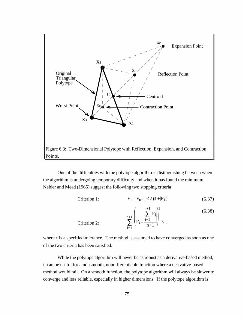
75
xe
xr
C
X1
X3X2
xcWorst Point
Expansion Point
Reflection Point
Centroid
Contraction Point
OriginalTriangularPolytope
Figure 6.3: Two-Dimensional Polytope with Reflection, Expansion, and Contraction
Points.
One of the difficulties with the polytope algorithm is distinguishing between when
the algorithm is undergoing temporary difficulty and when it has found the minimum.
Nelder and Mead (1965) suggest the following two stopping criteria
Criterion 1: F1 - Fn+1 ≤ ε 1+ F1 (6.37)
Criterion 2: Fi -
Fj∑j=1
n+1
n+1
2
∑i=1
n+1
≤ ε
(6.38)
where ε is a specified tolerance. The method is assumed to have converged as soon as one
of the two criteria has been satisfied.
While the polytope algorithm will never be as robust as a derivative-based method,
it can be useful for a nonsmooth, nondifferentiable function where a derivative-based
method would fail. On a smooth function, the polytope algorithm will always be slower to
converge and less reliable, especially in higher dimensions. If the polytope algorithm is

76
employed, significant enhancements can be made to the polytope algorithm on a case-by-
case basis.
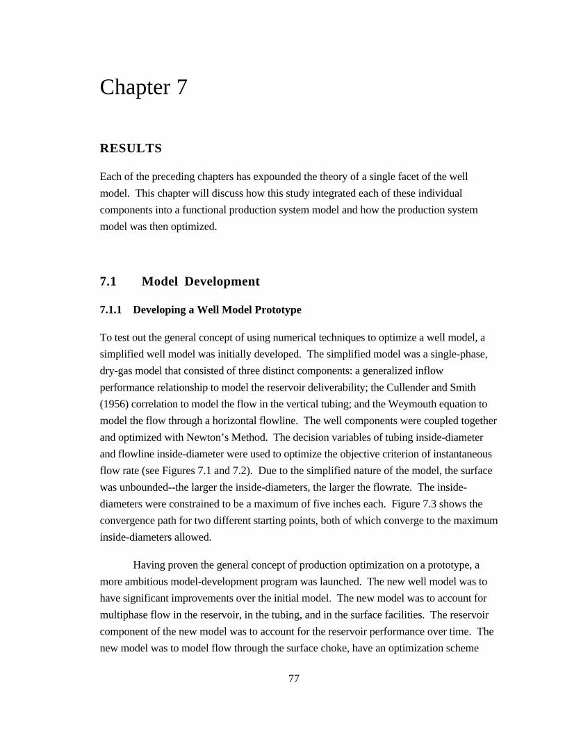
77
Chapter 7
RESULTS
Each of the preceding chapters has expounded the theory of a single facet of the well
model. This chapter will discuss how this study integrated each of these individual
components into a functional production system model and how the production system
model was then optimized.
7.1 Model Development
7.1.1 Developing a Well Model Prototype
To test out the general concept of using numerical techniques to optimize a well model, a
simplified well model was initially developed. The simplified model was a single-phase,
dry-gas model that consisted of three distinct components: a generalized inflow
performance relationship to model the reservoir deliverability; the Cullender and Smith
(1956) correlation to model the flow in the vertical tubing; and the Weymouth equation to
model the flow through a horizontal flowline. The well components were coupled together
and optimized with Newton’s Method. The decision variables of tubing inside-diameter
and flowline inside-diameter were used to optimize the objective criterion of instantaneous
flow rate (see Figures 7.1 and 7.2). Due to the simplified nature of the model, the surface
was unbounded--the larger the inside-diameters, the larger the flowrate. The inside-
diameters were constrained to be a maximum of five inches each. Figure 7.3 shows the
convergence path for two different starting points, both of which converge to the maximum
inside-diameters allowed.
Having proven the general concept of production optimization on a prototype, a
more ambitious model-development program was launched. The new well model was to
have significant improvements over the initial model. The new model was to account for
multiphase flow in the reservoir, in the tubing, and in the surface facilities. The reservoir
component of the new model was to account for the reservoir performance over time. The
new model was to model flow through the surface choke, have an optimization scheme
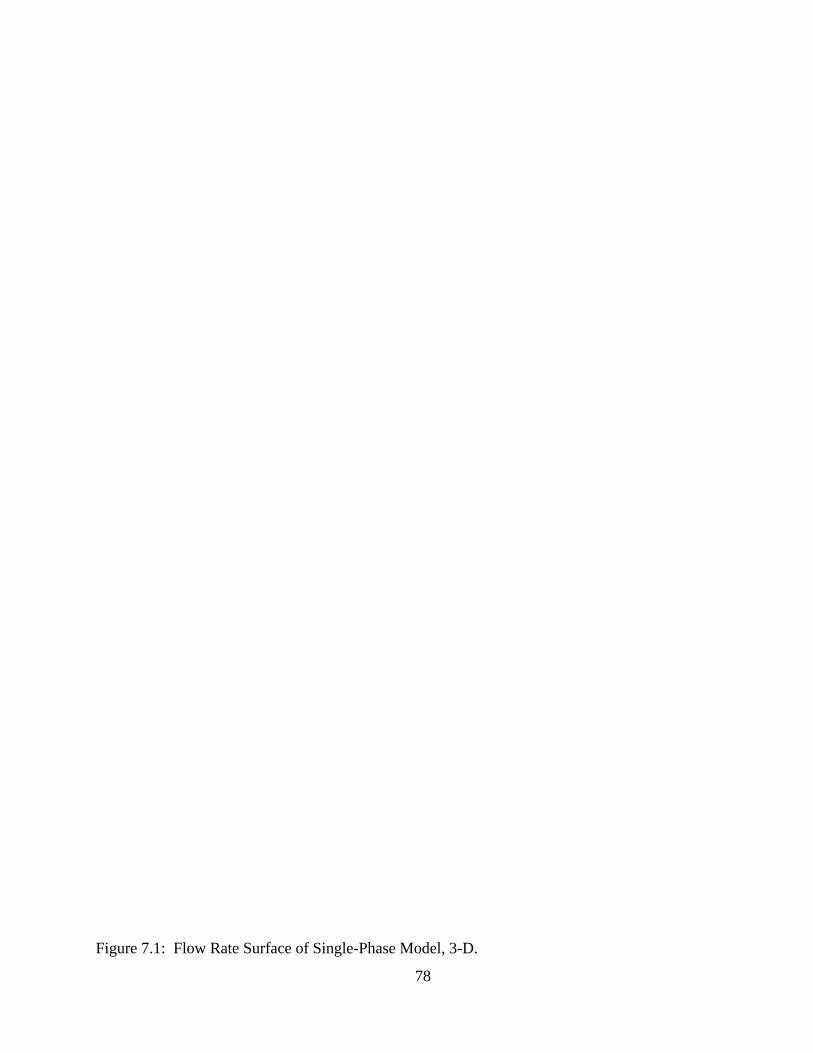
78
Figure 7.1: Flow Rate Surface of Single-Phase Model, 3-D.
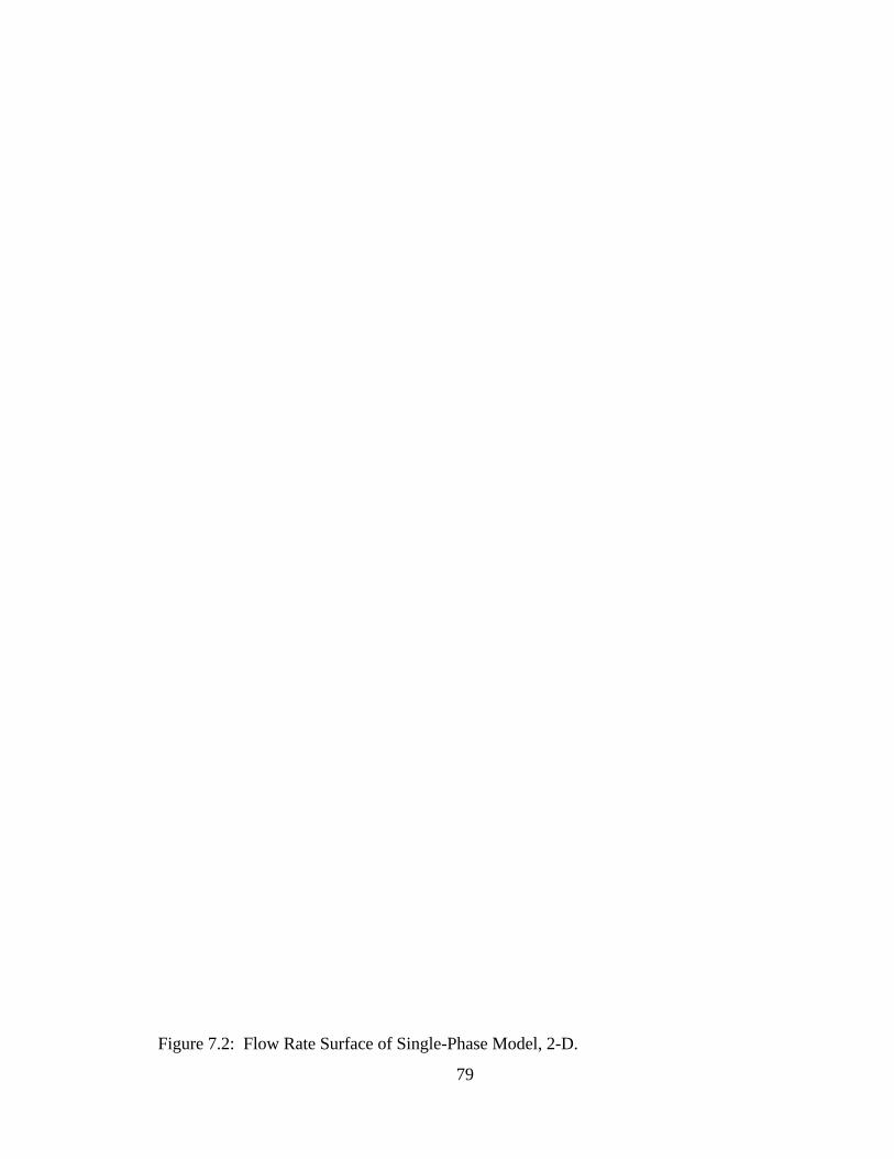
79
Figure 7.2: Flow Rate Surface of Single-Phase Model, 2-D.
80
Figure 7.3: Convergence Path of Single-Phase Model.

81
more stable than unmodified Newton’s Method, and was to optimize long-term financial
objectives.
7.1.2 Developing the Reservoir Component
To replicate the reservoir dynamics and inflow performance in the well model, this study
adopted a reservoir model developed by Borthne (1986) at the Norwegian Institute of
Technology, as discussed in Chapter 2. The reservoir model was originally designed with
just this purpose in mind--to provide a simple but functional reservoir component to be
included in a larger model. The model provides an accurate representation of constrained
reservoir performance that requires minimal computer processing. Borthne’s model is a
black-oil model that performs a generalized material balance calculation in concert with an
inflow performance relationship based on pseudopressure. The reservoir model is
constrained by both pressure and flowrate. In addition to specifying a minimum flowing
well pressure, two flowrates must be specified: a minimum flowrate and a maximum target
flowrate. The model attempts to satisfy the target flowrate without violating the minimum
flowing well pressure. For more details on the reservoir component used in the well
model, see Chapter 2.
7.1.3 Developing the Tubing Component
The next stage in the model development was to design and develop a component to model
the multiphase flow through the vertical flowstring. For this we relied on the many
empirical correlations that have been developed over the years. Three correlations were
selected to be included in the model. These were the modified Hagedorn & Brown
correlation (1965), the Orkiszewski correlation (1967), and the Aziz, Govier, and Fogarasi
correlation (1972). All three correlations are extensively used in the petroleum industry.
The Hagedorn and Brown (1965) correlation is one of the most empirical available, the
Aziz et al. (1972) correlation has the strongest theoretical basis.
Gradient maps of the three correlations were generated and are shown in Figures
7.4 through 7.9. Figures 7.4 and 7.5 show the gradient surface generated by the modified
Hagedorn and Brown (1965) correlation. The transition from the original Hagedorn and
Brown correlation, representing slug flow, to the Griffith & Wallis (1961) correlation,
representing bubble flow, is very distinct. Figures 7.6 and 7.7 show the Aziz et al. (1972)
correlation with their suggested flow map superimposed. Note theat the map appears
continuous everywhere except at the boundary between bubble flow and slug flow.
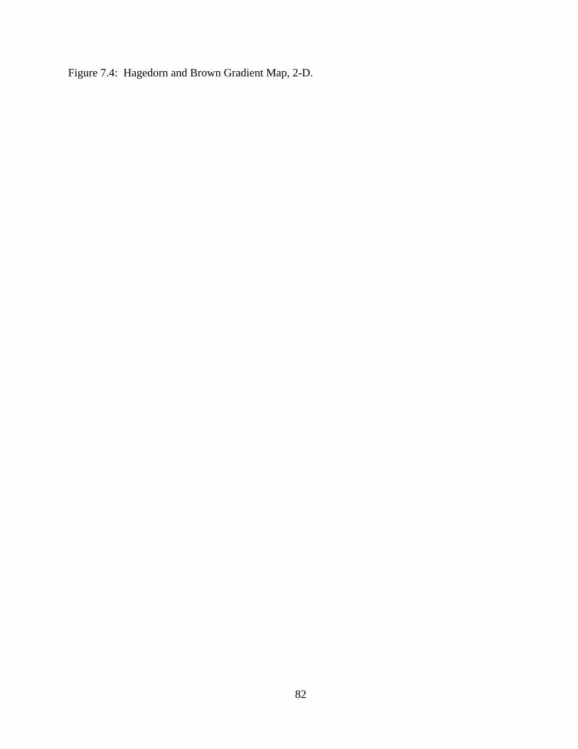
82
Figure 7.4: Hagedorn and Brown Gradient Map, 2-D.

83
Figure 7.5: Hagedorn and Brown Gradient Map, 3-D.

84
Figure 7.6: Aziz, Govier, and Fogarasi Gradient Map, 2-D.

85
Figure 7.7: Aziz, Govier, and Fogarasi Gradient Map, 3-D.

86
Figure 7.8: Orkeszewski Gradient Map, 2-D.

87
Figure 7.9: Orkeszewski Gradient Map, 3-D.
88
The Orkiszewski gradient maps appear in Figures 7.8 and 7.9. Here the boundaries
between all four flow regions are very distinct. For more information on the multiphase
flow component used in this well model, see Chapter 3.
7.1.4 Developing the Choke Component
After the reservoir and flowstring components were completed, we next developed a
component to model the surface choke. A surprising degree of difficulty was encountered
at this stage. Recall from Chapter 4 that a surface choke is a binary device: it operates in
either critical flow or subcritical flow. Also recall that in critical flow the flow rate through
the choke is independent of the downstream pressure. Thus a discontinuity occurs at the
critical-subcritical flow boundary. Since the well model was to be used in an iterative
fashion, the surface choke component would have to be applicable to all flow conditions,
both critical and subcritical. Much to our dismay, we discovered after researching the
techniques available that although good correlations are available for single phase flow
across chokes, good correlations for multiphase flow across chokes are rare. Of the
correlations that are available, most are strictly for critical flow.
Nodal analysis handles the surface choke discontinuity by avoiding it. In nodal
analysis, the separator pressure is specified and then related to the pressure downstream of
the choke by a horizontal flow correlation. Then the pressure drop across the choke is
obtained by assuming that the choke is always in critical flow and using an empirical
correlation. Notice that by specifying the downstream pressure and then calculating the
upstream pressure, this procedure manages to determine both the upstream and
downstream pressures in critical flow. If we specified the upstream pressure and tried to
determine the downstream pressure during critical flow, the best we can do is to ascertain
the maximum downstream pressure.
Assuming that the choke is always in critical flow was rejected as an option for this
well model. An attempt was made to devise a method to handle both critical and subcritical
flow. One of the few correlations to make an attempt at modeling both critical and
subcritical flow is the Sachdeva et al. (1986) choke model. With a few modifications to the
algorithm, the Sachdeva et al. (1986) model was able to be incorporated into the well
model. During critical flow through the choke, the downstream pressure was determined
by assuming the choke to be at the critical-subcritical boundary. This assumption allowed
the critical pressure ratio to determine the downstream pressure. See Chapter 4 for details.

89
The Sachdeva et al. (1986) model was developed and tested with the other
components of the well model. Figure 7.10 shows the present value surface generated by
the Sachdeva et al. (1986) model as a function of choke diameter and tubing diameter.
Notice that the critical-subcritical flow boundary occurs at a choke diameter of
approximately ten centimeters. Below this critical size, the surface is completely a function
of the choke diameter. Above the critical choke diameter, the surface is completely a
function of the tubing diameter. However, a physical constraint is required: the choke
diameter cannot be allowed to exceed the tubing diameter. This constraint is shown in
Figure 7.11.
Although we were able to successfully incorporate into the well model a choke
component that modeled both critical and subcritical flow, this was at great computational
expense. In addition, several of the assumptions in the choke model, such as no mass
transfer occurring between phases, were considered to be highly suspect. For these
reasons, we opted not to include a choke component in the well model.
7.1.5 Developing the Separation Component
The next stage was the development of a component to model surface facilities. We elected
to model the surface facilities with a two-stage separation process. A two-stage separation
process involves flashing the well stream initially at the separator operating conditions and
then flashing the resulting liquid stream at stock tank conditions. The flash calculation
implemented in this component is based on the Soave-Redlich-Kwong equation of state.
For more information on the phase separation component, see Chapter 5.
Thus, in its final state, the well model consists of a reservoir component, a
production string component, and a surface phase separation component. For any
combination of variables, the model will give the production profile for a given time step
and a given project life. In all examples cited here, a six-month time step and a 15 year
project life was used.
7.2 Defining the Objective Criterion
In order to perform optimization on the well model, the production profile had to be
transformed into an objective criterion. The objective criterion used in this research was the
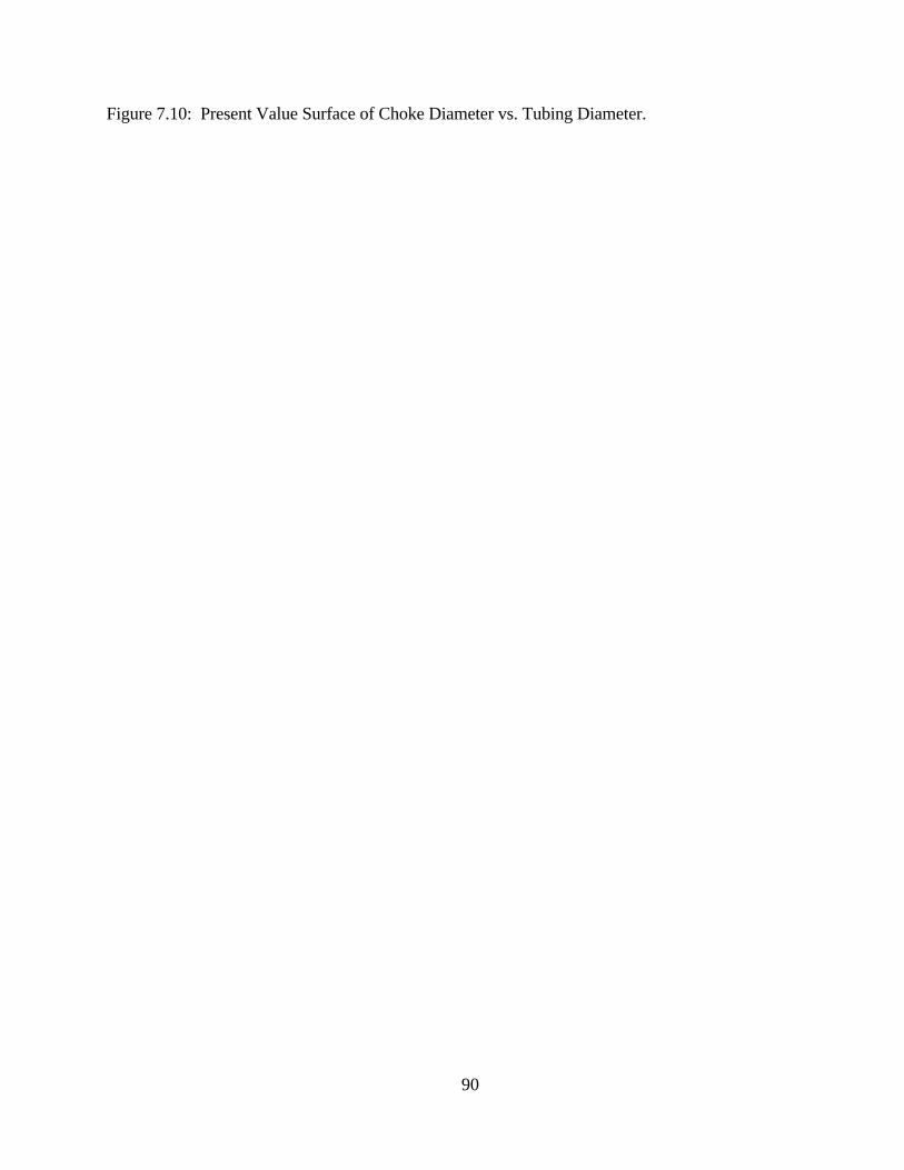
90
Figure 7.10: Present Value Surface of Choke Diameter vs. Tubing Diameter.

91
Figure 7.11: Constrained Present Value Surface of Choke Diameter vs. Tubing Diameter.
92
present value of the revenue stream generated over the life of the project. The present value
of the revenue stream is obtained by discounting the revenue stream over the life of the
project back to the present. The discounting scheme used in this model is relatively simple
and easy to follow. The model accounts for both the company’s cost of capital and the
expected inflation rate. Both of these parameters are assumed constant over the life of the
project.
A company has two primary means of securing capital from outside sources: the
issuance of equity in the company and the assumption of debt. A company’s cost of capital
is typically determined as a weighted average of the company’s cost of debt and the
company’s cost of equity. If we let
rD = interest rate of debt, fraction
rE = return on equity expected by shareholders, fraction
D = amount of long-term debt, $
E = amount of outstanding equity, $
TC = corporate tax rate, fraction
then the company’s cost of capital may be expressed as
r* = rD 1-TC DD+E
+ rE ED+E (7.1)
Typically a company’s executive management will specify the weighted-average cost of
capital to be used in financial calculations.
Knowing the cost of capital, r*, and the inflation rate, i, the discount rate, in real
terms, may be expressed as
R = 1+r*
1+i - 1 (7.2)
Thus both the effect of the cost of capital and the effect of inflation have been coupled into
one discount factor. Note that this discount factor, the real discount factor R, may only be
used with cash flow expressed in real terms.
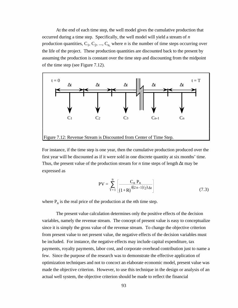
93
At the end of each time step, the well model gives the cumulative production that
occurred during a time step. Specifically, the well model will yield a stream of n
production quantities, C1, C2, ..., Cn, where n is the number of time steps occurring over
the life of the project. These production quantities are discounted back to the present by
assuming the production is constant over the time step and discounting from the midpoint
of the time step (see Figure 7.12).
t = T∆t ∆t ∆t ∆t ∆t
C1 C2 C3 Cn-1 Cn
t = 0
Figure 7.12: Revenue Stream is Discounted from Center of Time Step.
For instance, if the time step is one year, then the cumulative production produced over the
first year will be discounted as if it were sold in one discrete quantity at six months’ time.
Thus, the present value of the production stream for n time steps of length ∆t may be
expressed as
PV = Cn Pn
1+R 2 n -1 2 ∆t
∑T=1
n
(7.3)
where Pn is the real price of the production at the nth time step.
The present value calculation determines only the positive effects of the decision
variables, namely the revenue stream. The concept of present value is easy to conceptualize
since it is simply the gross value of the revenue stream. To change the objective criterion
from present value to net present value, the negative effects of the decision variables must
be included. For instance, the negative effects may include capital expenditure, tax
payments, royalty payments, labor cost, and corporate overhead contribution just to name a
few. Since the purpose of the research was to demonstrate the effective application of
optimization techniques and not to concoct an elaborate economic model, present value was
made the objective criterion. However, to use this technique in the design or analysis of an
actual well system, the objective criterion should be made to reflect the financial
94
ramifications as accurately as possible and therefore a criterion of net present value should
be used.
7.3 Results
7.3.1 The Surface of the Well Model
Once the well model was completed and the objective criterion was decided upon, a surface
map was generated of the objective criterion as a function of two decision variables.
Namely, the present value of the production stream was plotted as a function of the
separator pressure and the tubing diameter (see Figure 7.13). The surface appears to be a
textbook example of an optimization surface: nice, smooth contour lines bounding the
extreme value on all sides. However, closer inspection of the surface reveals a different
story. As shown in Figure 7.14, looking at a closer level reveals a surface that is very
rough and ill-behaved. The rough features were masked by the graphics software in Figure
7.13 but are plainly visible in Figure 7.14.
A better understanding of the surface can be obtained by examining several
unidimensional profiles. Figures 7.15 through 7.18 show four different profiles of the
surface. The first three figures keep the separator pressure constant while varying the
tubing diameter. It is clearly visible that the surface is very rough and discontinuous along
this dimension. Figure 7.17 shows the amount of noise present at the maximum of the
surface. Figure 7.18 is a profile of the other dimension. This profile was obtained by
holding the tubing diameter constant and varying the separator pressure. The figure shows
that in this dimension, the surface is a very smooth and continuous function. Thus, the
surface is rough as a function of tubing diameter and smooth as a function of separator
pressure.
This conclusion about the surface obtained from the profiles is reinforced by
investigating the derivatives of the function. Figures 7.19 and 7.20 show the first and
second derivatives of separator pressure. These derivatives clearly exhibit that the surface
is very smooth as a function of separator pressure (be advised that the two graphs are
shown from two different viewing angles). The smoothness of the function with respect to
separator pressure is very much in contrast to the roughness of the function with respect to
tubing diameter. Figures 7. 21 and 7.22 show the first and second derivatives of tubing
95
Figure 7.13: Present Value Surface of Separator Pressure vs. Tubing Diameter.

96
Figure 7.14: Rough Features of Present Value Surface.

97
Figure 7.15: Profile of Tubing Diameter for Constant Separator Pressure.
98
Figure 7.16: Close-up of Tubing Diameter Profile for Constant Separator Pressure.
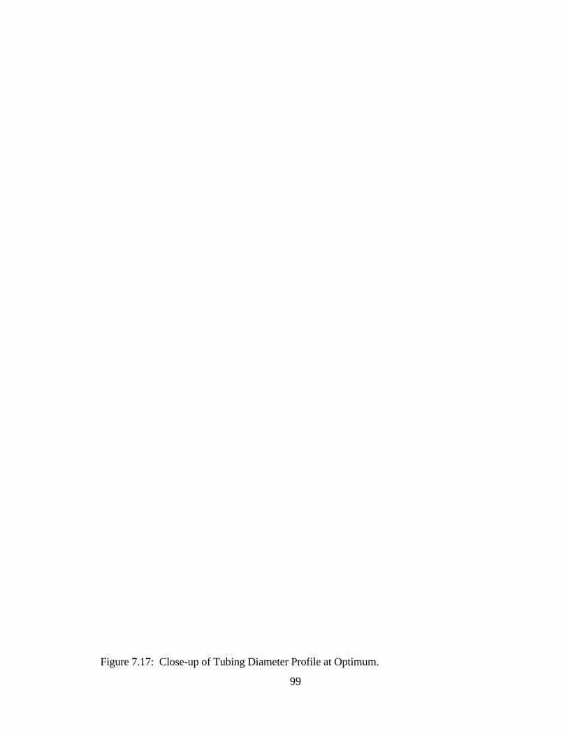
99
Figure 7.17: Close-up of Tubing Diameter Profile at Optimum.
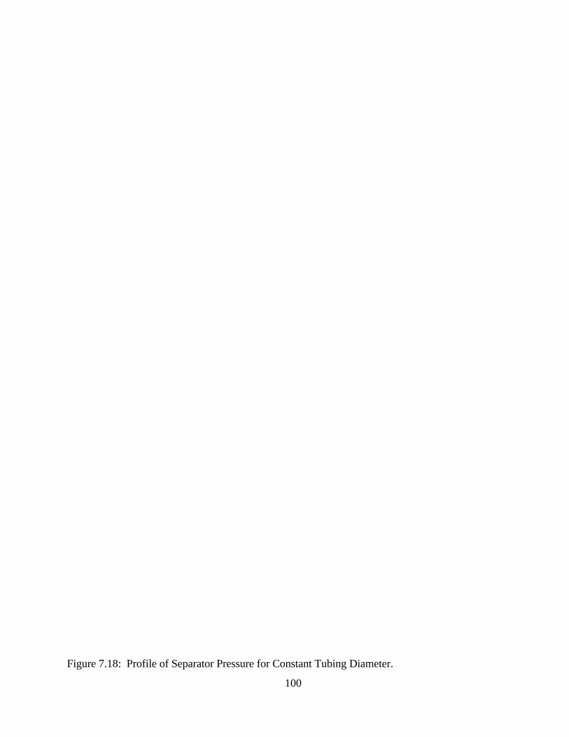
100
Figure 7.18: Profile of Separator Pressure for Constant Tubing Diameter.

101
Figure 7.19: First Derivative of Separator Pressure.
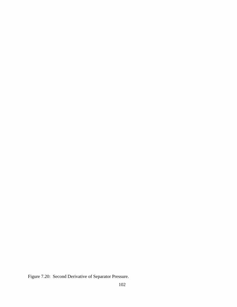
102
Figure 7.20: Second Derivative of Separator Pressure.
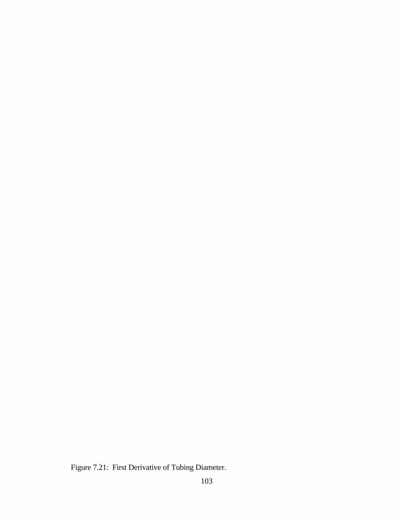
103
Figure 7.21: First Derivative of Tubing Diameter.

104
Figure 7.22: Second Derivative of Tubing Diameter.
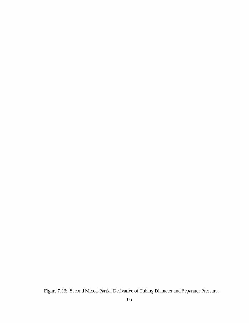
105
Figure 7.23: Second Mixed-Partial Derivative of Tubing Diameter and Separator Pressure.
106
diameter (again the graphs are shown from two different angles). The surface is very
discontinuous in the vicinity of the optimal tubing diameter. Figure 7.23 shows the second
mixed partial derivative. Note that the origin of this derivative coincides with the extreme
value of the surface.
Further insights to the function can be obtained by investigating the eigensystem of
the surface. Figures 7.24, 7.25, and 7.26 show the minimum eigenvalue of the surface,
the maximum eigenvalue of the surface, and the curvature of the surface. Notice that the
eigenvalues are negative. Going against the convention in optimization to always pose the
problem so that minimization is performed, this study has explicitly performed
maximization of the objective function by using a negative definite Hessian. Since the
Hessian is forced to be negative definite so that an ascent direction is assured, the
eigenvalues are negative in value. Since we are approximating the objective function with a
negative definite Hessian, regions of positive curvature indicate areas where Newton’s
Method may fail to converge. Note the similarity between these three graphs and the three
graphs of the second derivatives.
7.3.2 Performing Optimization on the Well Model
Having developed the well model and having analyzed the properties of the surface of the
decision variables, numerical optimization techniques were employed in an attempt to
maximize the function. Knowing that the surface is not smooth with respect to one of the
variables, we did not expect derivative-based optimization methods to perform very well on
the function.
Figure 7.27 shows the results of using unmodified Newton’s Method to optimize
the function. Shown on the figure are four different starting points that are all relatively
close to and equidistant from the desired solution. However, two of the starting points
resulted in convergence to the maximum value while two of the starting points resulted in
divergence. The difference between the four points becomes apparent by analyzing Figure
7.21, the graph showing the first derivative of the tubing diameter. Figure 7.21 shows a
trough occurring in the first derivative between a tubing diameter of eight to nine
centimeters. The trough in the first derivative of the tubing diameter represents an
inflection of the second-order surface. In essence this trough divides two distinct second
order surfaces. The two points that converged to the maximum were on one side of this
inflection while the two points that diverged were on the other side of the inflection. Recall
from Chapter 6 that unmodified Newton’s method simply makes a quadratic approximation

107
Figure 7.24: Minimum Eigenvalue of Hessian Matrix.

108
Figure 7.25: Maximum Eigenvalue of Hessian Matrix.

109
Figure 7.26: Curvature of Hessian Matrix.
110
to whatever the immediate second order surface happens to be. Since unmodified
Newton’s method does not force the solution to take a descent direction, the two points
which start at a tubing diameter of nine centimeters are attempting to converge to a
stationary point other than the desired stationary point. Thus, using unmodified Newton’s
Method, the initial guess must be on the proper side of this inflection to converge to the
desired stationary point.
We next tried optimizing the function with a modified form of Newton’s Method.
The algorithm employed was obtained from Dr. Walter Murray of the Stanford
Optimization Laboratory. The algorithm is described on pages 108-111 of Gill et al.
(1981) and is based on modified Cholesky factorization. The modification is very similar
to the Greenstadt modification discussed in Chapter 6 in that after it factors the Hessian to
obtain the diagonal, it forces the diagonal elements to be positive and greater than some
small value. The algorithm also employs a line search procedure to ensure that the optimal
step length is taken for a given search direction. As can be seen from Figure 7.28,
significant improvement was achieved in the convergence to the maximum value. Even
when the starting points were not near the solution, the method always converged to the
optimum solution.
Due to the unavailability of analytic derivatives, both of the Newton-based methods
determined the gradient and Hessian by using finite difference approximations. Since the
surface of the function is nonsmooth, obtaining meaningful derivatives was very difficult.
Critical in the performance of both methods was the size of the finite difference interval.
By taking relatively large finite difference intervals, we were able to mask the effects of the
nonsmooth surface. We found that taking finite differences of one-tenth of the size of the
decision variables produced good results.
As an alternative to derivative-based methods, the performance of the polytope
heuristic was investigated. As discussed in Chapter 6, the polytope heuristic is a direct
search method based on function comparisons and not on derivative information. The
performance of the polytope heuristic is shown in figures 7.29, 7.30, and 7.31. Measured
strictly on the number of function evaluations required to find the solution, the polytope
method took the equivalent of five iterations of Newton’s Method. Specifically, the
convergence path shown in Figure 7.29-7.31 required 45 function evaluations which is
equivalent to five iterations of a Newton-based method using a nine-point finite
differencing scheme.

111
Figure 7.27: Convergence Path of Unmodified Newton’s Method.

112
Figure 7.28: Convergence Path of Modified Newton’s Method.

113
Figure 7.29: Convergence Path of Polytope Heuristic, 2-D.
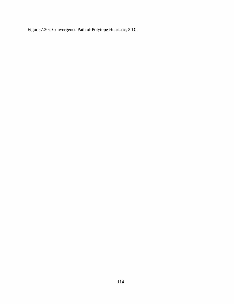
114
Figure 7.30: Convergence Path of Polytope Heuristic, 3-D.

115
Figure 7.31: Convergence Path of Triangular Polytopes.
117
Chapter 8
CONCLUSIONS
8.1 Conclusions
The emphasis of this study may be summarized by two key points:
1) Nonlinear optimization techniques can be successfully applied to
production system optimization.
2) Nonlinear optimization of a production system model is an intelligent
alternative to exhaustive iteration of a production system model.
The significant advantages of using nonlinear optimization in lieu of exhaustive iteration are
• Nonlinear optimization is not limited by the number of decision variables-
-an unlimited number of decision variables may be optimized
simultaneously. Exhaustive iteration is limited to one or two decision
variables and becomes intractable when three or more variables are
optimized, especially when the variables are interrelated.
• Nonlinear optimization may be used to optimize various objective criteria.
Examples of various objective criteria are: to maximize the present value
of the production stream, to maximize the net present value of the well,
to maximize cumulative recovery on an equivalent barrel basis, to
minimize the cumulative gas-oil ratio, to minimize the cumulative water-
oil ratio, to minimize total investment per equivalent barrel produced, to
maximize the rate-of-return of the well, etc.
118
• Nonlinear optimization may be used to optimize well conditions over a
span of time. This is best described by considering an example: for a ten-
year time span, nonlinear optimization will determine the optimal tubing
diameter to use each year--simply add ten decision variables, one for each
tubing size each year. As another example, if only three tubing changes
are allowed over the ten-year span, nonlinear optimization will determine
when the changes should be made and what size the tubing should be.
Attempting this with exhaustive iteration is ill-advised.
• Nonlinear optimization avoids the trial and error procedure of exhaustive
iteration. Nonlinear optimization based on Newton’s technique will
achieve quadratic convergence to the optimal solution.
This study investigated several different nonlinear optimization methods. The
significant findings are
• Unmodified Newton’s Method is not viable for optimization. This
technique is highly sensitive to the initial guess.
• The performance of Newton’s Method can be greatly improved by
including a line search procedure and a modification to ensure a direction
of descent.
• For nonsmooth functions, the polytope heuristic provides an effective
alternative to a derivative-based method.
• For nonsmooth functions, the finite difference approximations are greatly
affected by the size of the finite difference interval. This study found a
finite difference interval of one-tenth of the size of the variable to be
advisable.
8.2 Suggestions for Future Work
One idea that was flirted with briefly but is not included in this report is to revise the
implementation of classical nodal analysis. Current practitioners of nodal analysis use
exhaustive iteration to solve the system of equations that represents the well. Why not
119
formulate the problem to solve for the root of a system of nonlinear equations, namely by
using Newton’s Method? Simply set up the problem to contain a pressure residual at each
node and then use Newton’s Method to solve the equations for the stabilized flow rate.
Alternately, you could set up the problem to contain a flow rate residual at each node and
then use Newton’s Method to solve the equations for the stabilized pressure at the solution
node. Hence, you could use Newton’s Method for two different purposes in the
optimization of a production system: to solve for the zero of the function and then again to
solve for the zero of the gradient of the function.
Several improvements can be made to the current well model. Obviously, it would
be interesting to know why the model is nonsmooth with respect to tubing diameter. The
cause of this is not yet apparent. In addition, it would be nice to expand the model to
include a completion component that models the completion effects (perforations, gravel
pack, ....) and also a horizontal flow component that models the pressure loss and phase
segregation that occur in surface flowlines between the wellhead and the separator. It
would also be interesting to develop a well model based on a compositional equations
instead of black oil equations. In addition, one area where the current well model has
significant problems is with computational expense. A more efficient manner for solving
for the stabilized flow rate should be found.
Perhaps the biggest improvement would be to demonstrate the use of different
objective criteria in the optimization process. This would clearly demonstrate the inherent
advantages of nonlinear optimization over exhaustive iteration.
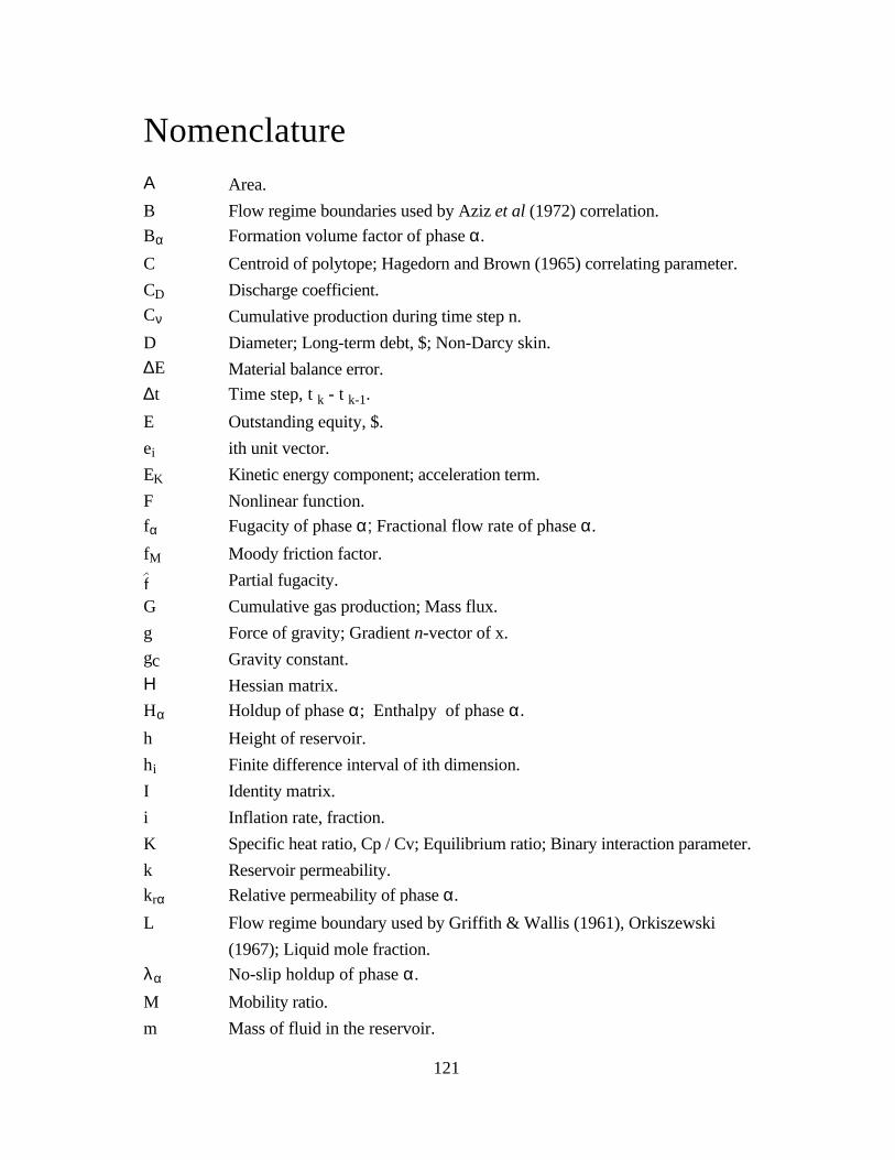
121
NomenclatureΑ Area.
B Flow regime boundaries used by Aziz et al (1972) correlation.
Bα Formation volume factor of phase α.
C Centroid of polytope; Hagedorn and Brown (1965) correlating parameter.
CD Discharge coefficient.
Cν Cumulative production during time step n.
D Diameter; Long-term debt, $; Non-Darcy skin.
∆E Material balance error.
∆t Time step, t k - t k-1.
E Outstanding equity, $.
ei ith unit vector.
EK Kinetic energy component; acceleration term.
F Nonlinear function.
fα Fugacity of phase α; Fractional flow rate of phase α.
fM Moody friction factor.
f Partial fugacity.
G Cumulative gas production; Mass flux.
g Force of gravity; Gradient n-vector of x.
gc Gravity constant.
Η Hessian matrix.
Hα Holdup of phase α; Enthalpy of phase α.h Height of reservoir.
hi Finite difference interval of ith dimension.
I Identity matrix.
i Inflation rate, fraction.
K Specific heat ratio, Cp / Cv; Equilibrium ratio; Binary interaction parameter.
k Reservoir permeability.
krα Relative permeability of phase α.
L Flow regime boundary used by Griffith & Wallis (1961), Orkiszewski
(1967); Liquid mole fraction.
λα No-slip holdup of phase α.
M Mobility ratio.
m Mass of fluid in the reservoir.

122
m(P) Gas pseudopressure.
N Cumulative oil production; Dimensionless groups defined by Ros (1961);
Flow regime parameter used by Aziz et al. (1972).
P Pressure; The n-vector of displacement from x; Newton search vector.
Pn Real price of the production at the nth time step
PV Present value.
Q Quadratic equation.
Q* Stabilized flow rate determined by nodal analysis.
q Volumetric flow rate.
q Mass flow rate.
R Universal gas constant; Real discount factor.
r* Cost of capital, fraction.
rD Interest rate of debt, fraction.
Re Reynold’s number.
rE Return on equity expected by shareholders, fraction.
re Radius of drainage.
RP Producing gas-liquid ratio.
RS Solution gas-oil ratio.
rS Solution oil-gas ratio.
rw Radius of wellbore.
S Darcy skin; Diameter of bean, 64ths of an inch.
Sα Saturation of phase α.
T Temperature.
TC Corporate tax rate, fraction.
V Volume; Velocity; Specific volume; Vapor mole fraction; Matrix of
eigenvectors.
Vα Velocity of phase α.
VΒ Bulk volume of the reservoir.
VBF Absolute bubble rise velocity.
VBS Bubble rise velocity.
VM Superficial velocity of the mix.
VSα Superficial velocity of phase α.
ωα Acentric factor of phase α.X Free gas quality; Oil composition.
x n-vector of decision variables.
xc Contraction point.

123
xe Expansion point.
xr Reflection point.
Y Pressure ratio, downstream to upstream pressure; Composition of gas.
Z Objective variable; depth in well; Composition of mixture.
Subscripts
1 Upstream.
2 Downstream.
BUB Bubble flow regime.
c Critical.
CH Choke.
F Friction.
G Gas.
GG Gas phase derived from gas phase.
GO Gas phase derived from oil phase.
HB Hagedorn and Brown.
HH Hydrostatic head.
i Gridblock position in x-direction.
j Gridblock position in y-direction.
K Iteration number.
KE Kinetic energy.
L Liquid.
M Mixture.
MIST Annular-mist flow regime.
NS No slip.
O Oil.
OG Oil phase derived from gas phase.
OO Oil phase derived from oil phase.
r Reduced.
S Slip.
SLUG Slug flow regime.
TRANS Transition flow regime.
W Water.
WE Weber.
WH Wellhead.
124
Superscript.“ Variable is normalized to reservoir bulk volume.L Liquid phase.R Reservoir conditions.S Standard conditions.T Transpose.V Vapor phase.
Greek Lettersα Reflection coefficient.
β Expansion coefficient .
ε Absolute pipe roughness; tolerance.
φ Reservoir porosity; Fugacity coefficient.
Φα Mechanical irreversibilities of phase α.
γ Contraction coefficient.
Λ Diagonal matrix of eigenvalues.
µ Marquardt parameter.
µα Viscosity of phase α.
ρ Newton step length.
ρα Density of phase α.
σ Interfacial tension.
ψ Hagedorn and Brown correlating parameter; Roots of cubic equation.
∇ Gradient.
∇ . Divergence.
125
Bibliography
[1] Achong, I.: “Revised Bean Performance Formula for Lake Maracaibo Wells,” Shell
Internal Report (Oct. 1961).
[2] Ali, H. M., Batchelor, A.S.J., Beale, E.M.L., and Beasley, J.F.: “Mathematical
Models to Help Manage the Oil Resources of Kuwait,” unpublished manuscript (1983).
[3] Amyx, J. W., Bass, D. M., and Whiting, R. L.: Petroleum Reservoir Engineering,
McGraw-Hill, New York (1960).
[4] Arnold, K., and Stewart, M.: Surface Production Operations: Design of Oil-Handling
Systems and Facilities, Gulf Publishing, Houston, 1 (1986).
[5] Aronofsky, J. S., and Lee, A. S.: “A Linear Programming Model for Scheduling
Crude Oil Production,” J. Petro. Tech. (July 1958) 51-54.
[6] Aronofsky, J. S., and Williams, A. C.: “The Use of Linear Programming and
Mathematical Models in Underground Oil Production,” Mgmt. Sci. 8 (1962) 394-407.
[7] Aronofsky, J. S.: “Optimization Methods in Oil and Gas Development,” paper
SPE12295, prepared for the J. Petro. Tech. (July 1983).
[8] Asheim, H. A.: “Offshore Petroleum Exploration Planning by Numerical Simulation
and Optimization,” Ph.D. dissertation, Dept. of Petro. Eng., University of Texas at Austin
(December 1978).
[9] Ashford, F. E., and Pierce, P. E.: “Determining Multiphase Pressure Drops and Flow
Capacities in Down-Hole Safety Valves,” J. Petro. Tech. (Sept. 1975) 1145-1152.
[10] Attra, H. D., Wise, H. B., and Black, W. M.: “Application of Optimizing Techniques
for Studying Field Producing Operations,” J. Petro. Tech. (January 1961) 82-86.
126
[11] Aziz, K., Govier, G.W., and Fogarasi, M.: “Pressure Drop in Wells Producing Oil
and Gas,” J. Canadian Petro. Tech. (July 1972) 38-48.
[12] Barua, J., Horne, R. N., Greenstadt, J. L., Lopez, L.: “Improved Estimation
Algorithms for Automated Type-Curve Analysis of Well Tests,” SPEFE (March 1988)
186-196.
[13] Barua, Jawahar.: A Study of Newton Related Nonlinear Methods in Well Test
Analysis, Production Schedule Optimization and Reservoir Simulation, PhD thesis,
Stanford University, (1989).
[14] Baxendall, P. B., and Thomas, R.: “The Calculation of Pressure Gradients in High-
Rate Flowing Wells,” J. Petro. Tech. (Oct. 1961) 1023-1028.
[15] Baxendall, P. B.: “Bean Performance--Lake Wells,” Internal Report (Oct. 1957).
[16] Beggs, H. D., and Brill, J. P.: “A Study of Two-Phase Flow in Inclined Pipes,” J.
Petro. Tech. (May 1973) 607-617.
[17] Bohannon, J. M.: “A Linear Programming Model for Optimum Development of Multi-
Reservoir Pipeline Systems,” J. Petro. Tech. (Nov. 1970) 1429-1436.
[18] Borthne, Gunnar.: A Simulation Model for Oil and Gas-condensate Production
Based on Material Balance and Inflow Performance Calculations, Norwegian Institute of
Technology (1986).
[19] Brill, J. P., and Beggs, H. D.: Two-Phase Flow in Pipes, Tulsa (1978).
[20] Brown, K. E., and Lea, James F.: “Nodal Systems Analysis of Oil and Gas Wells,”
J. Petro. Tech. (October 1985) 1751-63.
[21] Brown, K. E.: The Technology of Artificial Lift Methods, 1 and 4, Penwell Publishing
Co., Tulsa (1977).
[22] Broyden, C. G.: “The Convergence of a Class of Double Rank Minimization
Algorithms. 2. The New Algorithm,” J. Inst. Math. Appl. (1970) 6, 221-31.
127
[23] Charnes, A., and Cooper, W. W.: Management Models and Industrial Applications
of Linear Programming, Vol. II, John Wiley & Sons, NY (1961).
[24] Chu, M. H., and Evans, R. D.: “Production System Optimization for Natural Fowing
Water Drive Wells,” SPE Paper 11582, presented at the 1983 Production Operation
Symposium, Oklahoma City, Feb 27 - March 1.
[25] Coats, K. H.: “An Approach to Locating New Wells in Heterogeneous, Gas
Producing Fields,” J. Petro. Tech. (May 1969) 549-558.
[26] Crichlow, H. B.: Modern Reservoir Engineering--A Simulation Approach, Prentice-
Hall, Englewood Cliffs, NJ (1977).
[27] Cullender, M. H., and Smith, R. V.: “Practical Solution of Gas Flow Equations for
Wells and Pipelines with Large Temperature Gradients,” Trans. AIME (1956) 207.
[28] Duns, H., and Ros, N. C. J.: “Vertical Flow of Gas and Liquid Mixtures in Wells,”
Proc., 6th World Petro. Congress (1963) 451-465.
[29] Fancher, G. H., and Brown, K. E.: “Prediction of Pressure Gradients for Multiphase
Flow in Tubing,” SPEJ (March 1963) 59-69.
[30] Fortunati, F.: “Two Phase Flow Through Wellhead Chokes,” SPE Paper 3742
presented at the 1972 SPE European Meeting, Amsterdam, May 17-18.
[31] Gilbert, W. E.: “Flowing and Gas-lift Well Performance,” Drill. and Prod. Prac.,
API (1954) 126.
[32] Gill, Philip E., Murray, Walter, and Wright, Margaret H.: Practical Optimization,
Academic Press, New York (1981).
[33] Golan, M., and Whitson, C. H.: Well Performance, IHRDC, Boston (1986).
[34] Govier, G. W., and Aziz, K.: The Flow of Complex Mixtures in Pipes, Van Nostrand
Reinhold Co., New York City (1972).
128
[35] Greenstadt, J. L.: “On the Relative Efficiencies of Gradient Methods,” Mathematics of
Computation, 21 (1967) 360-67.
[36] Gregory, M., Aziz, K., and Fogarasi, M.: “Analysis of Vertical Two-Phase Flow
Calculations, Crude Oil, Gas Flow in Well Tubing,” J. Canad. Petro. Tech. (Jan 1980) 86-
92.
[37] Griffith, P., and Wallis, G. B.: “Two-Phase Slug Flow,” J. Heat Transfer, ASME
(Aug. 1961) 307-320.
[38] Guzhov, A. J., and Medeiediev, V. F.: “Critical Flow of Two-Phase Liquids Through
Wellhead Chokes,” Nieftianoie Xoziastva-Moskva No. 11 (1962) in Russian.
[39] Hagedorn, A. R., and Brown, K. E.: “Experimental Study of Pressure Gradients
Occurring During Continuous Two-Phase Flow in Small-Diameter Vertical Conduits,” J.
Petro. Tech. (April 1965) 475-484.
[40] Hazim, S. H. Al-Najjar, and Nimat, B. Abu Al-Soof: “Alternative Flow-Pattern Maps
Can Improve Pressure-Drop Calculations of the Aziz et al. Multiphase-Flow Correlation,”
SPEPE (August 1989) 327-334.
[41] Hunt, J. L.: “Production-Systems Analysis for Fractured Wells,” SPEPE (Nov.
1988) 608-614.
[42] Huppler, J. D.: “Scheduling Gas Field Production for Maximum Profit,” SPEJ (June
1974) 274-279.
[43] IMSL Inc., IMSL MATH/LIBRARY User’s Manual, 3, Chapter 8, IMSL, Houston
(1987).
[44] Kuller, R. G., and Cummings, R. G.: “An Economic Model for Investment and
Production for Petroleum Reservoirs,” Am. Econ. Rev. 64 (1974) 66-79.
[45] Lang, Z. X., and Horne, R. N.: “Optimum Production Scheduling Using Reservoir
Simulators: A Comparison of Linear Programming and Dynamic Programming

129
Techniques,” SPE Paper 12159, presented at the 1983 SPE Annual Technical Conference
and Exhibition, San Francisco, October 5-8.
[46] Lasdon, L., Coffman, P. E., MacDonald, R., McFarland, J. W., and Sepehrnoori,
K.: “Optimal Hydrocarbon Reservoir Production Policies,” Operations Research (Jan.
1986) 34, 40-54.
[47] Lea, J. F., and Brown, K. E.: “Production Optimization Using a Computerized Well
Model,” SPE Paper 14121, presented at the SPE 1986 International Meeting on Petroleum
Engineering, Beijing (March 1986).
[48] Marquardt, D. W.: “An Algorithm for Least-Squares Estimation of Nonlinear
Parameters,” J. SIAM (June 1963) 11, No. 2, 431-41.
[49] McFarland, J. W., Lasdon, L., and Loose, V.: “Development Planning and
Management of Petroleum Reservoirs Using Tank Models and Nonlinear Programming,”
Operations Research (Mar. 1984) 32, 270-289.
[50] Murray, J. E., III, and Edgar, T. F.: “Optimal Scheduling of Production and
Compression in Gas Fields,” J. Petro. Tech. (Jan. 1979) 109-116.
[51] Nelder, J. A., and Mead, R.: “A Simplex Method for Function Minimization,”
Computer Journal 7, 308-313.
[52] O’Dell, P. M., Steubing, N. W., and Gray, J. W.: “Optimization of Gas Field
Operation,” J. Petro. Tech. (April 1973) 419-425.
[53] Omana, R. et al.: “Multiphase Flow Through Chokes,” SPE Paper 2682 presented at
the 1969 SPE Annual Meeting, Denver, Sept. 28 - Oct. 1.
[54] Orkiszewski, J.: “Predicting Two-Phase Pressure Drops in Vertical Pipes,” J. Petro.
Tech. (June 1967) 829-838.
[55] Poettman, F. H., and Carpenter, P. G.: “The Multiphase Flow of Gas, Oil and Water
Through Vertical Flow Strings with Application to the Design of Gas Lift Installations,”
Drill. and Prod. Prac., API (1952) 257-317.
130
[56] Poettmann, F. H., and Beck, R. L.: “New Charts Developed to Predict Gas-Liquid
Flow Through Chokes,” World Oil (March 1963) 95-101.
[57] Prausnitz, John M., Lichtenthaler, Ruediger N., and Gomes, Edmundo.: Molecular
Thermodynamics of Fluid-Phase Equilibria, Prentice Hall, Englewood Cliffs (1986).
[58] Press, W. H., Flannery, B. P., Teukolsky, S. A., and Vetterling, W. T.: Numerical
Recipes: The Art of Scientific Computing, Cambridge Press, Cambridge (1989).
[59] Ros, N. C. J.: “Simultaneous Flow of Gas and Liquid as Encountered in Well
Tubing,” J. Petro. Tech. (Oct. 1961) 1037.
[60] Ros, N. C. J.: “An Analysis of Critical Simultaneous Gas-Liquid Flow Through a
Restriction and its Application to Flow Metering,” Applied Sci. Research, 2 (1960) 374.
[61] Ros, N. C. J.: “Theoretical Approach to the Study of Critical Gas Flow through
Beans,” Shell Internal Report (Feb. 1959).
[62] Rosenwald, G. W., and Green, D. W.: “A Method for Determining the Optimal
Location of Wells in a Reservoir Using Mixed-Integer Programming,” SPEJ (Feb. 1974)
44-54.
[63] Rowan, G., and Warren, J. E.: “A Systems Approach to Reservoir Engineering,
Optimum Development Planning,” J. Canad. Petro. Tech. (July 1967) 84-94.
[64] Sachdeva, R., Schmidt, Z., Brill, J. P., and Blais, R. M.: “Two-Phase Flow
Through Chokes,” SPE Paper 15657, presented at the 1986 SPE Annual Technical
Conference and Exhibition, New Orleans, October 5-8.
[65] See, B. A., and Horne, R. N.: “Improved Application of Linear Programming
Optimization to Nonlinear Reservoir Simulations Using a Least-Squares Determination of
the Influence Functions,” SPEJ (Oct. 1983) 717-726.
[66] Soave, G.: Chem. Eng. Sci., 27, 1197 (1972).
131
[67] Strang, G.: Introduction to Applied Mathematics, Wellesley-Cambridge Press,
Wellesley, Mass. (1986).
[68] Tangeren, R. E. et al.: “Compressibility Effects of Two-Phase Flow,” J. App.
Physics, 20 (1949).
[69] Wattenbarger, R. A.: “Maximizing Seasonal Withdrawals from Gas Storage
Reservoirs,” J. Petro. Tech. (August 1970) 994-998.
[70] Weymouth equation
[71] Wilson, G. M., and Deal, C. H.: Ind. Eng. Chem. Fundam., 1: 20 (1962).

133
APPENDIX
Source Code for Well Model
![Simulated annealing type algorithms for multivariate ...mitter/publications/63_simulated_multi_ALG.pdf · Simulated Annealing Type Algorithms for Multivariate Optimization 421 [8],](https://img.dokumen.tips/doc/110x75/5e95c4db6a3a5365dd7475c5/simulated-annealing-type-algorithms-for-multivariate-mitterpublications63simulatedmultialgpdf.jpg)