Embed Size (px)
Citation preview
Example 1: Optimization Problem
a1
a 2
−5 −4 −3 −2 −1 0 1 2 3 4 5−5
0
5
J. McNames Portland State University ECE 4/557 Multivariate Optimization Ver. 1.14 3
Overview of Multivariate Optimization Topics
• Problem definition
• Algorithms
– Cyclic coordinate method
– Steepest descent
– Conjugate gradient algorithms
– PARTAN
– Newton’s method
– Levenberg-Marquardt
• Concise, subjective summary
J. McNames Portland State University ECE 4/557 Multivariate Optimization Ver. 1.14 1
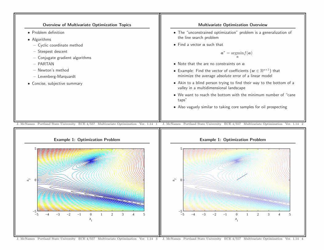
Example 1: Optimization Problem
a1
a 2
−5 −4 −3 −2 −1 0 1 2 3 4 5−5
0
5
J. McNames Portland State University ECE 4/557 Multivariate Optimization Ver. 1.14 4
Multivariate Optimization Overview
• The “unconstrained optimization” problem is a generalization ofthe line search problem
• Find a vector a such that
a∗ = argmina
f(a)
• Note that the are no constraints on a
• Example: Find the vector of coefficients (w ∈ Rp×1) that
minimize the average absolute error of a linear model
• Akin to a blind person trying to find their way to the bottom of avalley in a multidimensional landscape
• We want to reach the bottom with the minimum number of “canetaps”
• Also vaguely similar to taking core samples for oil prospecting
J. McNames Portland State University ECE 4/557 Multivariate Optimization Ver. 1.14 2
Example 1: Optimization Problem
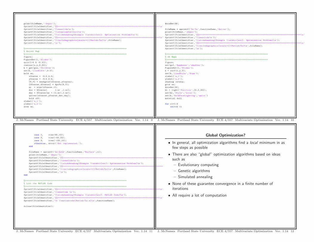
J. McNames Portland State University ECE 4/557 Multivariate Optimization Ver. 1.14 7
Example 1: Optimization Problem
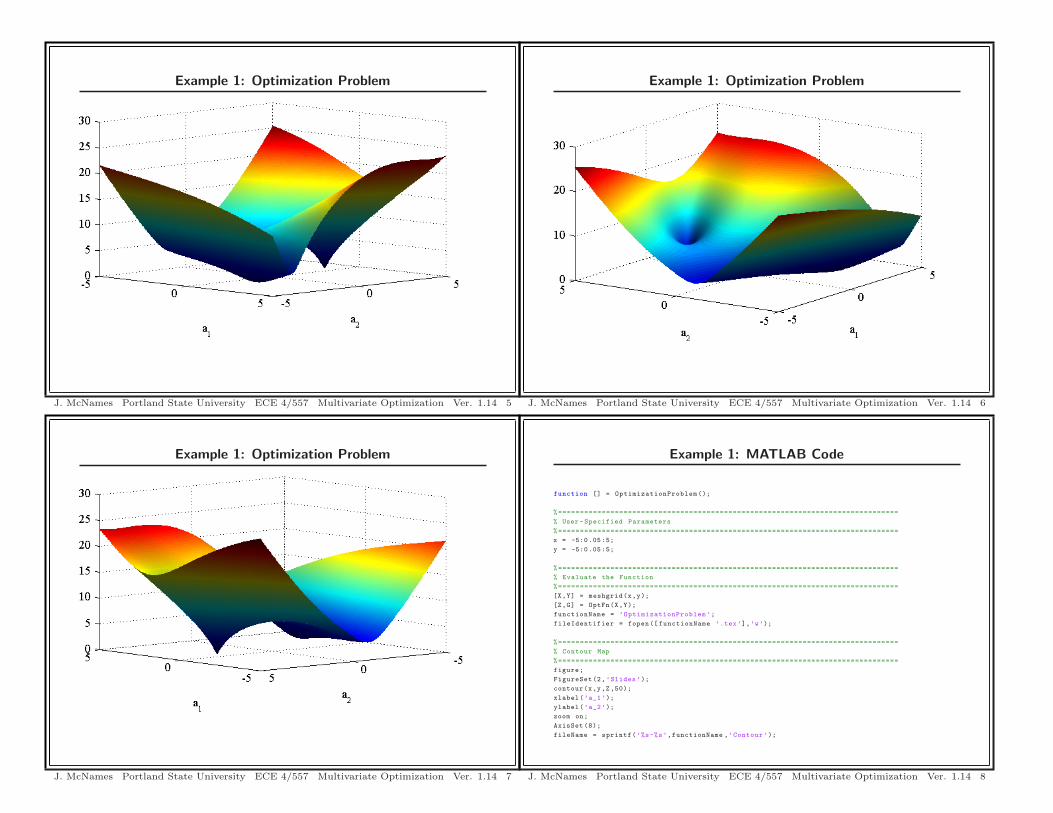
J. McNames Portland State University ECE 4/557 Multivariate Optimization Ver. 1.14 5
Example 1: MATLAB Code
function [] = OptimizationProblem ();
%==============================================================================
% User -Specified Parameters
%==============================================================================
x = -5:0.05 :5;
y = -5:0.05 :5;
%==============================================================================
% Evaluate the Function
%==============================================================================
[X,Y] = meshgrid(x,y);
[Z,G] = OptFn(X,Y);
functionName = ’OptimizationProblem ’;
fileIdentifier = fopen([ functionName ’.tex’],’w’);
%==============================================================================
% Contour Map
%==============================================================================
figure;
FigureSet(2,’Slides’);
contour(x,y,Z ,50);
xlabel(’a_1’);
ylabel(’a_2’);
zoom on;
AxisSet (8);
fileName = sprintf(’%s-%s’,functionName ,’Contour ’);
J. McNames Portland State University ECE 4/557 Multivariate Optimization Ver. 1.14 8
Example 1: Optimization Problem
J. McNames Portland State University ECE 4/557 Multivariate Optimization Ver. 1.14 6
case 1, view (45 ,10);
case 2, view ( -55 ,22);
case 3, view ( -131 ,10);
otherwise , error(’Not implemented. ’);
end
fileName = sprintf(’%s-%s%d’,functionName ,’Surface ’,c1);
print(fileName ,’-depsc’);
fprintf(fileIdentifier ,’%%=============================================================================
fprintf(fileIdentifier ,’\\ newslide\n’);
fprintf(fileIdentifier ,’\\ slideheading{Example \\ arabic{exc}: Optimization Problem }\n’);
fprintf(fileIdentifier ,’%%=============================================================================
fprintf(fileIdentifier ,’\\ includegraphics[scale =1]{ Matlab/%s}\n’,fileName );
fprintf(fileIdentifier ,’\n’);
end
%==============================================================================
% List the MATLAB Code
%==============================================================================
fprintf(fileIdentifier ,’%%==============================================================================\ n’
fprintf(fileIdentifier ,’\\ newslide \n’);
fprintf(fileIdentifier ,’\\ slideheading{Example \\ arabic{exc}: MATLAB Code}\n’);
fprintf(fileIdentifier ,’%%==============================================================================\ n’
fprintf(fileIdentifier ,’\t \\ matlabcode{Matlab/%s.m}\n’,functionName );
fclose(fileIdentifier );
J. McNames Portland State University ECE 4/557 Multivariate Optimization Ver. 1.14 11
print(fileName ,’-depsc’);
fprintf(fileIdentifier ,’%%==============================================================================\ n’
fprintf(fileIdentifier ,’\\ newslide\n’);
fprintf(fileIdentifier ,’\\ stepcounter{exc}\n’);
fprintf(fileIdentifier ,’\\ slideheading{Example \\ arabic{exc}: Optimization Problem }\n’);
fprintf(fileIdentifier ,’%%==============================================================================\ n’
fprintf(fileIdentifier ,’\\ includegraphics[scale =1]{ Matlab/%s}\n’,fileName );
fprintf(fileIdentifier ,’\n’);
%==============================================================================
% Quiver Map
%==============================================================================
figure;
FigureSet(1,’Slides’);
axis([-5 5 -5 5]);
contour(x,y,Z ,50);
h = get(gca ,’Children ’);
set(h,’LineWidth ’,0.2);
hold on;
xCoarse = -5:0.5:5;
yCoarse = -5:0.5:5;
[X,Y] = meshgrid(xCoarse ,yCoarse );
[ZCoarse ,GCoarse] = OptFn(X,Y);
nr = size(xCoarse ,1);
dzx = GCoarse( 1:nr ,1:nr);
dzy = GCoarse(nr + (1:nr),1:nr);
quiver(xCoarse ,yCoarse ,dzx ,dzy);
hold off;
xlabel(’a_1’);
ylabel(’a_2’);
zoom on;
J. McNames Portland State University ECE 4/557 Multivariate Optimization Ver. 1.14 9
Global Optimization?
• In general, all optimization algorithms find a local minimum in asfew steps as possible
• There are also “global” optimization algorithms based on ideassuch as
– Evolutionary computing
– Genetic algorithms
– Simulated annealing
• None of these guarantee convergence in a finite number ofiterations
• All require a lot of computation
J. McNames Portland State University ECE 4/557 Multivariate Optimization Ver. 1.14 12
AxisSet (8);
fileName = sprintf(’%s-%s’,functionName ,’Quiver’);
print(fileName ,’-depsc’);
fprintf(fileIdentifier ,’%%==============================================================================\ n’
fprintf(fileIdentifier ,’\\ newslide\n’);
fprintf(fileIdentifier ,’\\ slideheading{Example \\ arabic{exc}: Optimization Problem }\n’);
fprintf(fileIdentifier ,’%%==============================================================================\ n’
fprintf(fileIdentifier ,’\\ includegraphics[scale =1]{ Matlab/%s}\n’,fileName );
fprintf(fileIdentifier ,’\n’);
%==============================================================================
% 3D Maps
%==============================================================================
figure;
set(gcf ,’Renderer ’,’zbuffer ’);
FigureSet(1,’Slides’);
h = surf(x,y,Z);
set(h,’LineStyle ’,’None’);
xlabel(’a_1’);
ylabel(’a_2’);
shading interp;
grid on;
AxisSet (8);
hl = light(’Position ’ ,[0,0,30]);
set(hl ,’Style’,’Local’);
set(h,’BackFaceLighting ’,’unlit’)
material dull
for c1=1:3
switch c1
J. McNames Portland State University ECE 4/557 Multivariate Optimization Ver. 1.14 10

Cyclic Coordinate Method
1. For i = 1 to p,
ai := argminα
f([a1, a2, . . . , ai−1, α, ai+1, . . . , ap])
2. Loop to 1 until convergence
+ Simple to implement
+ Each line search can be performed semi-globally to avoid shallowlocal minima
+ Can be used with nominal variables
+ f(a) can be discontinuous
+ No gradient required
− Very slow compared to gradient-based optimization algorithms
− Usually only practical when the number of parameters, p, is small
• There are modified versions with faster convergence
J. McNames Portland State University ECE 4/557 Multivariate Optimization Ver. 1.14 15
Optimization Comments
• Ideally, when we construct models we should favor those whichcan be optimized with few shallow local minima and reasonablecomputation
• Graphically you can think of the function to be minimized as theelevation in a complicated high-dimensional landscape
• The problem is to find the lowest point
• The most common approach is to go downhill
• The gradient points in the most “uphill” direction
• The steepest downhill direction is the opposite of the gradient
• Most optimization algorithms use a line search algorithm
• The methods mostly differ only in the way that the “direction ofdescent” is generated
J. McNames Portland State University ECE 4/557 Multivariate Optimization Ver. 1.14 13
Example 2: Cyclic Coordinate Method
−5 0 5−5
−4
−3
−2
−1
0
1
2
3
4
5
X
Y
J. McNames Portland State University ECE 4/557 Multivariate Optimization Ver. 1.14 16
Optimization Algorithm Outline
• The basic steps of these algorithms is as follows
1. Pick a starting vector a
2. Find the direction of descent, d
3. Move in that direction until a minimum is found:
α∗ := argminα
f(a + αd)
a := a + α∗d
4. Loop to 2 until convergence
• Most of the theory of these algorithms is based on quadraticsurfaces
• Near local minima, this is a good approximation
• Note that the functions should (must) have continuous gradients(almost) everywhere
J. McNames Portland State University ECE 4/557 Multivariate Optimization Ver. 1.14 14

Example 2: Cyclic Coordinate Method
0 5 10 15 20 250
1
2
3
4
5
6
Iteration
Euc
lidea
n Po
sitio
n E
rror
J. McNames Portland State University ECE 4/557 Multivariate Optimization Ver. 1.14 19
Example 2: Cyclic Coordinate Method
−3 −2 −1 0−3.5
−3
−2.5
−2
−1.5
−1
−0.5
0
0.5
X
Y
J. McNames Portland State University ECE 4/557 Multivariate Optimization Ver. 1.14 17
Example 2: Relevant MATLAB Code
function [] = CyclicCoordinate ();
%clear all;
close all;
ns = 26;
x = -3;
y = 1;
b0 = -1;
ls = 30;
a = zeros(ns ,2);
f = zeros(ns ,1);
[z,dzx ,dzy] = OptFn(x,y);
a(1,:) = [x y];
f(1) = z;
for cnt = 2:ns,
if rem(cnt ,2)==1 ,
d = [1 0]’; % Along x direction
else
d = [0 1]’; % Along y direction
end;
[b,fmin] = LineSearch ([x y]’,d,b0 ,ls);
x = x + b*d(1);
y = y + b*d(2);
J. McNames Portland State University ECE 4/557 Multivariate Optimization Ver. 1.14 20
Example 2: Cyclic Coordinate Method
0 5 10 15 20 250
1
2
3
4
5
6
7
Iteration
Func
tion
Val
ue
J. McNames Portland State University ECE 4/557 Multivariate Optimization Ver. 1.14 18
print -depsc CyclicCoordinateContourB;
figure;
FigureSet (2,4.5 ,2.75);
k = 1:ns;
xerr = (sum (((a-ones(ns ,1)*[ xopt2 yopt2])’).^2)’).^(1/2);
h = plot(k-1,xerr ,’b’);
set(h(1),’Marker’,’.’);
set(h,’MarkerSize ’ ,6);
xlabel(’Iteration ’);
ylabel(’Euclidean Position Error’);
xlim ([0 ns -1]);
ylim ([0 xerr (1)]);
grid on;
set(gca ,’Box’,’Off’);
AxisSet (8);
print -depsc CyclicCoordinatePositionError;
figure;
FigureSet (2,4.5 ,2.75);
k = 1:ns;
h = plot(k-1,f,’b’ ,[0 ns],zopt *[1 1],’r’ ,[0 ns],zopt2 *[1 1],’g’);
set(h(1),’Marker’,’.’);
set(h,’MarkerSize ’ ,6);
xlabel(’Iteration ’);
ylabel(’Function Value’);
ylim ([0 f(1)]);
xlim ([0 ns -1]);
grid on;
set(gca ,’Box’,’Off’);
AxisSet (8);
J. McNames Portland State University ECE 4/557 Multivariate Optimization Ver. 1.14 23
a(cnt ,:) = [x y];
f(cnt) = fmin;
end;
[x,y] = meshgrid (0+( -0 .01:0.001:0.01),3+(-0.01:0 .001:0.01 ));
[z,dzx ,dzy] = OptFn(x,y);
[zopt ,id1] = min(z);
[zopt ,id2] = min(zopt);
id1 = id1(id2);
xopt = x(id1 ,id2);
yopt = y(id1 ,id2);
[x,y] = meshgrid (1 .883+(-0.02:0.001:0.02),-2.963+(-0.02:0.001:0.02 ));
[z,dzx ,dzy] = OptFn(x,y);
[zopt2 ,id1] = min(z);
[zopt2 ,id2] = min(zopt2);
id1 = id1(id2);
xopt2 = x(id1 ,id2);
yopt2 = y(id1 ,id2);
figure;
FigureSet (1,4.5 ,2.75);
[x,y] = meshgrid (-5:0.1:5,-5:0.1 :5);
z = OptFn(x,y);
contour(x,y,z ,50);
h = get(gca ,’Children ’);
set(h,’LineWidth ’,0.2);
axis(’square’);
hold on;
h = plot(a(:,1),a(:,2),’k’,a(:,1),a(:,2),’r’);
J. McNames Portland State University ECE 4/557 Multivariate Optimization Ver. 1.14 21
print -depsc CyclicCoordinateErrorLinear;
J. McNames Portland State University ECE 4/557 Multivariate Optimization Ver. 1.14 24
set(h(1),’LineWidth ’,1.2);
set(h(2),’LineWidth ’,0.6);
h = plot(xopt ,yopt ,’kx’,xopt ,yopt ,’rx’);
set(h(1),’LineWidth ’,1.5);
set(h(2),’LineWidth ’,0.5);
set(h(1),’MarkerSize ’ ,5);
set(h(2),’MarkerSize ’ ,4);
hold off;
xlabel(’X’);
ylabel(’Y’);
zoom on;
AxisSet (8);
print -depsc CyclicCoordinateContourA;
figure;
FigureSet (1,4.5 ,2.75);
[x,y] = meshgrid (-1.5 + (-2:0.05:2),-1.5 + (-2:0.05 :2));
[z,dzx ,dzy] = OptFn(x,y);
contour(x,y,z ,75);
h = get(gca ,’Children ’);
set(h,’LineWidth ’,0.2);
axis(’square’);
hold on;
h = plot(a(:,1),a(:,2),’k’,a(:,1),a(:,2),’r’);
set(h(1),’LineWidth ’,1.2);
set(h(2),’LineWidth ’,0.6);
hold off;
xlabel(’X’);
ylabel(’Y’);
zoom on;
AxisSet (8);
J. McNames Portland State University ECE 4/557 Multivariate Optimization Ver. 1.14 22

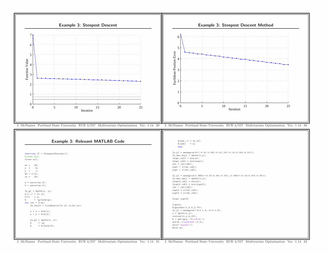
Example 3: Steepest Descent
−5 0 5−5
−4
−3
−2
−1
0
1
2
3
4
5
X
Y
J. McNames Portland State University ECE 4/557 Multivariate Optimization Ver. 1.14 27
Steepest Descent
The gradient of the function f(a) is defined as the vector of partialderivatives:
∇af(a) ≡[
∂f(a)∂a1
∂f(a)∂a2
. . . ∂f(a)∂ap
]T
• It can be shown that the gradient, ∇af(a), “points” in thedirection of maximum ascent
• The negative of the gradient, −∇af(a), “points” in the directionof maximum descent
• A vector d is a direction of descent if there exists a ε such thatf(a + λd) < f(a) for all 0 < λ < ε
• It can also be shown that d is a direction of descent iff(∇af(a))
T
d < 0
• The algorithm of steepest descent uses d = −∇af(a)
• The most fundamental of all algorithms for minimizing acontinuously differentiable function
J. McNames Portland State University ECE 4/557 Multivariate Optimization Ver. 1.14 25
Example 3: Steepest Descent
−2 −1.8 −1.6 −1.4 −1.2−2.2
−2.1
−2
−1.9
−1.8
−1.7
−1.6
−1.5
−1.4
−1.3
−1.2
X
Y
J. McNames Portland State University ECE 4/557 Multivariate Optimization Ver. 1.14 28
Steepest Descent
+ Very stable algorithm
− Can converge very slowly once near the local minima where thesurface is approximately quadratic
J. McNames Portland State University ECE 4/557 Multivariate Optimization Ver. 1.14 26
Example 3: Relevant MATLAB Code
function [] = SteepestDescent ();
%clear all;
close all;
ns = 26;
x = -3;
y = 1;
b0 = 0.01;
ls = 30;
a = zeros(ns ,2);
f = zeros(ns ,1);
[z,g] = OptFn(x, y);
a(1,:) = [x y];
f(1) = z;
d = -g/norm(g);
for cnt = 2:ns,
[b,fmin] = LineSearch ([x y]’,d,b0 ,ls);
x = x + b*d(1);
y = y + b*d(2);
[z,g] = OptFn(x, y);
d = -g;
d = d/norm(d);
J. McNames Portland State University ECE 4/557 Multivariate Optimization Ver. 1.14 31
Example 3: Steepest Descent
0 5 10 15 20 250
1
2
3
4
5
6
7
Iteration
Func
tion
Val
ue
J. McNames Portland State University ECE 4/557 Multivariate Optimization Ver. 1.14 29
a(cnt ,:) = [x y];
f(cnt) = z;
end;
[x,y] = meshgrid (0+( -0 .01:0.001:0.01),3+(-0.01:0 .001:0.01 ));
[z,dzx ,dzy] = OptFn(x,y);
[zopt ,id1] = min(z);
[zopt ,id2] = min(zopt);
id1 = id1(id2);
xopt = x(id1 ,id2);
yopt = y(id1 ,id2);
[x,y] = meshgrid (1 .883+(-0.02:0.001:0.02),-2.963+(-0.02:0.001:0.02 ));
[z,dzx ,dzy] = OptFn(x,y);
[zopt2 ,id1] = min(z);
[zopt2 ,id2] = min(zopt2);
id1 = id1(id2);
xopt2 = x(id1 ,id2);
yopt2 = y(id1 ,id2);
[zopt zopt2]
figure;
FigureSet (1,4.5 ,2.75);
[x,y] = meshgrid (-5:0.1:5,-5:0.1 :5);
z = OptFn(x,y);
contour(x,y,z ,50);
h = get(gca ,’Children ’);
set(h,’LineWidth ’,0.2);
axis(’square’);
hold on;
J. McNames Portland State University ECE 4/557 Multivariate Optimization Ver. 1.14 32
Example 3: Steepest Descent Method
0 5 10 15 20 250
1
2
3
4
5
6
Iteration
Euc
lidea
n Po
sitio
n E
rror
J. McNames Portland State University ECE 4/557 Multivariate Optimization Ver. 1.14 30
AxisSet (8);
print -depsc SteepestDescentErrorLinear ;
J. McNames Portland State University ECE 4/557 Multivariate Optimization Ver. 1.14 35
h = plot(a(:,1),a(:,2),’k’,a(:,1),a(:,2),’r’);
set(h(1),’LineWidth ’,1.2);
set(h(2),’LineWidth ’,0.6);
h = plot(xopt ,yopt ,’kx’,xopt ,yopt ,’rx’);
set(h(1),’LineWidth ’,1.5);
set(h(2),’LineWidth ’,0.5);
set(h(1),’MarkerSize ’ ,5);
set(h(2),’MarkerSize ’ ,4);
hold off;
xlabel(’X’);
ylabel(’Y’);
zoom on;
AxisSet (8);
print -depsc SteepestDescentContourA;
figure;
FigureSet (1,4.5 ,2.75);
[x,y] = meshgrid (-1.6 + (-0.5:0.01:0.5),-1.7 + (-0.5:0.01:0.5));
z = OptFn(x,y);
contour(x,y,z ,75);
h = get(gca ,’Children ’);
set(h,’LineWidth ’,0.2);
axis(’square’);
hold on;
h = plot(a(:,1),a(:,2),’k’,a(:,1),a(:,2),’r’);
set(h(1),’LineWidth ’,1.2);
set(h(2),’LineWidth ’,0.6);
hold off;
xlabel(’X’);
ylabel(’Y’);
zoom on;
J. McNames Portland State University ECE 4/557 Multivariate Optimization Ver. 1.14 33
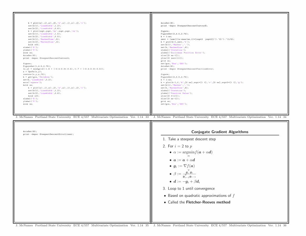
Conjugate Gradient Algorithms
1. Take a steepest descent step
2. For i = 2 to p
• α := argminα
f(a + αd)
• a := a + αd
• gi := ∇f(a)
• β := gTi gi
gTi−1gi−1
• d := −gi + βdi
3. Loop to 1 until convergence
• Based on quadratic approximations of f
• Called the Fletcher-Reeves method
J. McNames Portland State University ECE 4/557 Multivariate Optimization Ver. 1.14 36
AxisSet (8);
print -depsc SteepestDescentContourB;
figure;
FigureSet (2,4.5 ,2.75);
k = 1:ns;
xerr = (sum (((a-ones(ns ,1)*[ xopt2 yopt2])’).^2)’).^(1/2);
h = plot(k-1,xerr ,’b’);
set(h(1),’Marker’,’.’);
set(h,’MarkerSize ’ ,6);
xlabel(’Iteration ’);
ylabel(’Euclidean Position Error’);
xlim ([0 ns -1]);
ylim ([0 xerr (1)]);
grid on;
set(gca ,’Box’,’Off’);
AxisSet (8);
print -depsc SteepestDescentPositionError;
figure;
FigureSet (2,4.5 ,2.75);
k = 1:ns;
h = plot(k-1,f,’b’ ,[0 ns],zopt *[1 1],’r’ ,[0 ns],zopt2 *[1 1],’g’);
set(h(1),’Marker’,’.’);
set(h,’MarkerSize ’ ,6);
xlabel(’Iteration ’);
ylabel(’Function Value’);
ylim ([0 f(1)]);
xlim ([0 ns -1]);
grid on;
set(gca ,’Box’,’Off’);
J. McNames Portland State University ECE 4/557 Multivariate Optimization Ver. 1.14 34

Example 4: Fletcher-Reeves Conjugate Gradient
0 5 10 15 20 250
1
2
3
4
5
6
7
Iteration
Func
tion
Val
ue
J. McNames Portland State University ECE 4/557 Multivariate Optimization Ver. 1.14 39
Example 4: Fletcher-Reeves Conjugate Gradient
−5 0 5−5
−4
−3
−2
−1
0
1
2
3
4
5
X
Y
J. McNames Portland State University ECE 4/557 Multivariate Optimization Ver. 1.14 37
Example 4: Fletcher-Reeves Conjugate Gradient
0 5 10 15 20 250
1
2
3
4
5
6
Iteration
Euc
lidea
n Po
sitio
n E
rror
J. McNames Portland State University ECE 4/557 Multivariate Optimization Ver. 1.14 40
Example 4: Fletcher-Reeves Conjugate Gradient
1.5 2 2.5−3.5
−3.4
−3.3
−3.2
−3.1
−3
−2.9
−2.8
−2.7
−2.6
−2.5
X
Y
J. McNames Portland State University ECE 4/557 Multivariate Optimization Ver. 1.14 38

h = plot(a(:,1),a(:,2),’k’,a(:,1),a(:,2),’r’);
set(h(1),’LineWidth ’,1.2);
set(h(2),’LineWidth ’,0.6);
h = plot(xopt ,yopt ,’kx’,xopt ,yopt ,’rx’);
set(h(1),’LineWidth ’,1.5);
set(h(2),’LineWidth ’,0.5);
set(h(1),’MarkerSize ’ ,5);
set(h(2),’MarkerSize ’ ,4);
hold off;
xlabel(’X’);
ylabel(’Y’);
zoom on;
AxisSet (8);
print -depsc FletcherReevesContourA;
figure;
FigureSet (1,4.5 ,2.75);
[x,y] = meshgrid (1.5:0.01:2.5 ,-3.5:0.01:-2.5);
z = OptFn(x,y);
contour(x,y,z ,75);
h = get(gca ,’Children ’);
set(h,’LineWidth ’,0.2);
axis(’square’);
hold on;
h = plot(a(:,1),a(:,2),’k’,a(:,1),a(:,2),’r’);
set(h(1),’LineWidth ’,1.2);
set(h(2),’LineWidth ’,0.6);
hold off;
xlabel(’X’);
ylabel(’Y’);
zoom on;
J. McNames Portland State University ECE 4/557 Multivariate Optimization Ver. 1.14 43
Example 4: Relevant MATLAB Code
function [] = FletcherReeves ();
%clear all;
close all;
ns = 26;
x = -3;
y = 1;
b0 = 0.01;
ls = 30;
a = zeros(ns ,2);
f = zeros(ns ,1);
[z,g] = OptFn(x, y);
a(1,:) = [x y];
f(1) = z;
d = -g/norm(g); % First direction
for cnt = 2:ns,
[b,fmin] = LineSearch ([x y]’,d,b0 ,ls);
x = x + b*d(1);
y = y + b*d(2);
go = g; % Old gradient
[z,g] = OptFn(x, y);
beta = (g’*g)/(go ’*go);
J. McNames Portland State University ECE 4/557 Multivariate Optimization Ver. 1.14 41
AxisSet (8);
print -depsc FletcherReevesContourB;
figure;
FigureSet (2,4.5 ,2.75);
k = 1:ns;
xerr = (sum (((a-ones(ns ,1)*[ xopt2 yopt2])’).^2)’).^(1/2);
h = plot(k-1,xerr ,’b’);
set(h(1),’Marker’,’.’);
set(h,’MarkerSize ’ ,6);
xlabel(’Iteration ’);
ylabel(’Euclidean Position Error’);
xlim ([0 ns -1]);
ylim ([0 xerr (1)]);
grid on;
set(gca ,’Box’,’Off’);
AxisSet (8);
print -depsc FletcherReevesPositionError;
figure;
FigureSet (2,4.5 ,2.75);
k = 1:ns;
h = plot(k-1,f,’b’ ,[0 ns],zopt *[1 1],’r’ ,[0 ns],zopt2 *[1 1],’g’);
set(h(1),’Marker’,’.’);
set(h,’MarkerSize ’ ,6);
xlabel(’Iteration ’);
ylabel(’Function Value’);
ylim ([0 f(1)]);
xlim ([0 ns -1]);
grid on;
set(gca ,’Box’,’Off’);
J. McNames Portland State University ECE 4/557 Multivariate Optimization Ver. 1.14 44
d = -g + beta*d;
a(cnt ,:) = [x y];
f(cnt) = z;
end;
[x,y] = meshgrid (0+( -0 .01:0.001:0.01),3+(-0.01:0 .001:0.01 ));
[z,dzx ,dzy] = OptFn(x,y);
[zopt ,id1] = min(z);
[zopt ,id2] = min(zopt);
id1 = id1(id2);
xopt = x(id1 ,id2);
yopt = y(id1 ,id2);
[x,y] = meshgrid (1 .883+(-0.02:0.001:0.02),-2.963+(-0.02:0.001:0.02 ));
[z,dzx ,dzy] = OptFn(x,y);
[zopt2 ,id1] = min(z);
[zopt2 ,id2] = min(zopt2);
id1 = id1(id2);
xopt2 = x(id1 ,id2);
yopt2 = y(id1 ,id2);
figure;
FigureSet (1,4.5 ,2.75);
[x,y] = meshgrid (-5:0.1:5,-5:0.1 :5);
z = OptFn(x,y);
contour(x,y,z ,50);
h = get(gca ,’Children ’);
set(h,’LineWidth ’,0.2);
axis(’square’);
hold on;
J. McNames Portland State University ECE 4/557 Multivariate Optimization Ver. 1.14 42

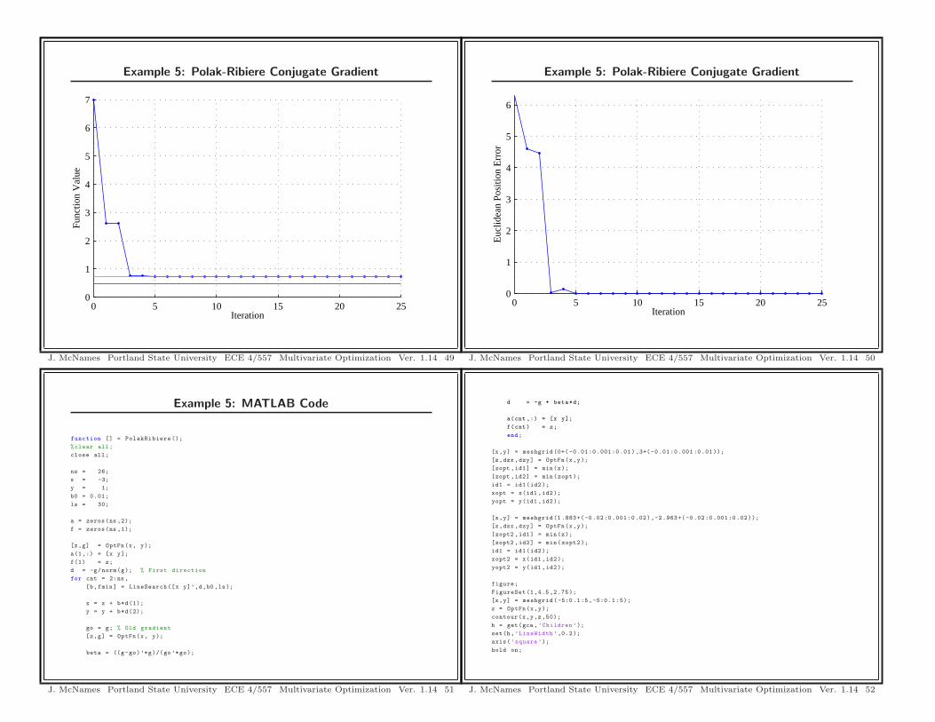
Example 5: Polak-Ribiere Conjugate Gradient
−5 0 5−5
−4
−3
−2
−1
0
1
2
3
4
5
X
Y
J. McNames Portland State University ECE 4/557 Multivariate Optimization Ver. 1.14 47
AxisSet (8);
print -depsc FletcherReevesErrorLinear;
J. McNames Portland State University ECE 4/557 Multivariate Optimization Ver. 1.14 45
Example 5: Polak-Ribiere Conjugate Gradient
1.5 2 2.5−3.5
−3.4
−3.3
−3.2
−3.1
−3
−2.9
−2.8
−2.7
−2.6
−2.5
X
Y
J. McNames Portland State University ECE 4/557 Multivariate Optimization Ver. 1.14 48
Conjugate Gradient Algorithms Continued
• There is also a variant called Polak-Ribiere where
β :=(gi − gi−1)
Tgi
gT
i−1gi−1
+ Only requires the gradient
+ Converges in a finite No. steps when f(a) is quadratic and perfectline searches are used
− Less stable numerically than steepest descent
− Sensitive to inexact line searches
J. McNames Portland State University ECE 4/557 Multivariate Optimization Ver. 1.14 46
Example 5: MATLAB Code
function [] = PolakRibiere ();
%clear all;
close all;
ns = 26;
x = -3;
y = 1;
b0 = 0.01;
ls = 30;
a = zeros(ns ,2);
f = zeros(ns ,1);
[z,g] = OptFn(x, y);
a(1,:) = [x y];
f(1) = z;
d = -g/norm(g); % First direction
for cnt = 2:ns,
[b,fmin] = LineSearch ([x y]’,d,b0 ,ls);
x = x + b*d(1);
y = y + b*d(2);
go = g; % Old gradient
[z,g] = OptFn(x, y);
beta = ((g-go)’*g)/(go ’*go);
J. McNames Portland State University ECE 4/557 Multivariate Optimization Ver. 1.14 51
Example 5: Polak-Ribiere Conjugate Gradient
0 5 10 15 20 250
1
2
3
4
5
6
7
Iteration
Func
tion
Val
ue
J. McNames Portland State University ECE 4/557 Multivariate Optimization Ver. 1.14 49
d = -g + beta*d;
a(cnt ,:) = [x y];
f(cnt) = z;
end;
[x,y] = meshgrid (0+( -0 .01:0.001:0.01),3+(-0.01:0 .001:0.01 ));
[z,dzx ,dzy] = OptFn(x,y);
[zopt ,id1] = min(z);
[zopt ,id2] = min(zopt);
id1 = id1(id2);
xopt = x(id1 ,id2);
yopt = y(id1 ,id2);
[x,y] = meshgrid (1 .883+(-0.02:0.001:0.02),-2.963+(-0.02:0.001:0.02 ));
[z,dzx ,dzy] = OptFn(x,y);
[zopt2 ,id1] = min(z);
[zopt2 ,id2] = min(zopt2);
id1 = id1(id2);
xopt2 = x(id1 ,id2);
yopt2 = y(id1 ,id2);
figure;
FigureSet (1,4.5 ,2.75);
[x,y] = meshgrid (-5:0.1:5,-5:0.1 :5);
z = OptFn(x,y);
contour(x,y,z ,50);
h = get(gca ,’Children ’);
set(h,’LineWidth ’,0.2);
axis(’square’);
hold on;
J. McNames Portland State University ECE 4/557 Multivariate Optimization Ver. 1.14 52
Example 5: Polak-Ribiere Conjugate Gradient
0 5 10 15 20 250
1
2
3
4
5
6
Iteration
Euc
lidea
n Po
sitio
n E
rror
J. McNames Portland State University ECE 4/557 Multivariate Optimization Ver. 1.14 50

AxisSet (8);
print -depsc PolakRibiereErrorLinear;
J. McNames Portland State University ECE 4/557 Multivariate Optimization Ver. 1.14 55
h = plot(a(:,1),a(:,2),’k’,a(:,1),a(:,2),’r’);
set(h(1),’LineWidth ’,1.2);
set(h(2),’LineWidth ’,0.6);
h = plot(xopt ,yopt ,’kx’,xopt ,yopt ,’rx’);
set(h(1),’LineWidth ’,1.5);
set(h(2),’LineWidth ’,0.5);
set(h(1),’MarkerSize ’ ,5);
set(h(2),’MarkerSize ’ ,4);
hold off;
xlabel(’X’);
ylabel(’Y’);
zoom on;
AxisSet (8);
print -depsc PolakRibiereContourA;
figure;
FigureSet (1,4.5 ,2.75);
[x,y] = meshgrid (1.5:0.01:2.5 ,-3.5:0.01:-2.5);
z = OptFn(x,y);
contour(x,y,z ,75);
h = get(gca ,’Children ’);
set(h,’LineWidth ’,0.2);
axis(’square’);
hold on;
h = plot(a(:,1),a(:,2),’k’,a(:,1),a(:,2),’r’);
set(h(1),’LineWidth ’,1.2);
set(h(2),’LineWidth ’,0.6);
hold off;
xlabel(’X’);
ylabel(’Y’);
zoom on;
J. McNames Portland State University ECE 4/557 Multivariate Optimization Ver. 1.14 53
Parallel Tangents (PARTAN)
1. First gradient step
• d := ∇f(a)
• α := argminα f(a + αd)
• sp := αd
• a := a + sp
2. Gradient Step
• dg := ∇f(a)
• α := argminα f(a + αd)
• sg := αd
• a := a + sg
3. Conjugate Step
• dp := sp + sg
• α := argminα f(a + αd)
• sp := αd
• a := a + sp
4. Loop to 2 until convergence
J. McNames Portland State University ECE 4/557 Multivariate Optimization Ver. 1.14 56
AxisSet (8);
print -depsc PolakRibiereContourB;
figure;
FigureSet (2,4.5 ,2.75);
k = 1:ns;
xerr = (sum (((a-ones(ns ,1)*[ xopt2 yopt2])’).^2)’).^(1/2);
h = plot(k-1,xerr ,’b’);
set(h(1),’Marker’,’.’);
set(h,’MarkerSize ’ ,6);
xlabel(’Iteration ’);
ylabel(’Euclidean Position Error’);
xlim ([0 ns -1]);
ylim ([0 xerr (1)]);
grid on;
set(gca ,’Box’,’Off’);
AxisSet (8);
print -depsc PolakRibierePositionError;
figure;
FigureSet (2,4.5 ,2.75);
k = 1:ns;
h = plot(k-1,f,’b’ ,[0 ns],zopt *[1 1],’r’ ,[0 ns],zopt2 *[1 1],’g’);
set(h(1),’Marker’,’.’);
set(h,’MarkerSize ’ ,6);
xlabel(’Iteration ’);
ylabel(’Function Value’);
ylim ([0 f(1)]);
xlim ([0 ns -1]);
grid on;
set(gca ,’Box’,’Off’);
J. McNames Portland State University ECE 4/557 Multivariate Optimization Ver. 1.14 54

Example 6: PARTAN
1.5 2 2.5−3.5
−3.4
−3.3
−3.2
−3.1
−3
−2.9
−2.8
−2.7
−2.6
−2.5
X
Y
J. McNames Portland State University ECE 4/557 Multivariate Optimization Ver. 1.14 59
PARTAN Concept
a0
a1
a2a3
a4
a5
a6 a7
• First two steps are steepest descent
• Thereafter, each iteration consists of two steps
1. Search along the direction
di = ai − ai−2
where ai is the current point and ai−2 is the point from twosteps ago
2. Search in the direction of the negative gradient
di = −∇f(ai)
J. McNames Portland State University ECE 4/557 Multivariate Optimization Ver. 1.14 57
Example 6: PARTAN
0 5 10 15 20 250
1
2
3
4
5
6
7
Iteration
Func
tion
Val
ue
J. McNames Portland State University ECE 4/557 Multivariate Optimization Ver. 1.14 60
Example 6: PARTAN
−5 0 5−5
−4
−3
−2
−1
0
1
2
3
4
5
X
Y
J. McNames Portland State University ECE 4/557 Multivariate Optimization Ver. 1.14 58

cnt = 2;
while cnt <ns ,
% Gradient step
[z,g] = OptFn(x,y);
d = -g/norm(g); % Direction
[bg ,fmin] = LineSearch ([x y]’,d,b0 ,ls);
xg = x + bg*d(1);
yg = y + bg*d(2);
cnt = cnt + 1;
a(cnt ,:) = [xg yg];
f(cnt) = OptFn(xg ,yg);
fprintf(’G : %d %5.3f\n’,cnt ,f(cnt ));
if cnt==ns,
break;
end;
% Conjugate
d = [xg -xa yg -ya]’;
if norm(d)�=0,
d = d/norm(d);
[bp ,fmin] = LineSearch ([xg yg]’,d,b0 ,ls);
else
bp = 0;
end;
if bp >0, % Line search in conjugate direction was successful
fprintf(’P :’);
x = xg + bp*d(1);
y = yg + bp*d(2);
J. McNames Portland State University ECE 4/557 Multivariate Optimization Ver. 1.14 63
Example 6: PARTAN
0 5 10 15 20 250
1
2
3
4
5
6
Iteration
Euc
lidea
n Po
sitio
n E
rror
J. McNames Portland State University ECE 4/557 Multivariate Optimization Ver. 1.14 61
else % Could not move - do another gradient update
cnt = cnt + 1;
a(cnt ,:) = a(cnt -1 ,:);
f(cnt) = f(cnt -1);
if cnt==ns ,
break;
end;
fprintf(’G2:’);
[z,g] = OptFn(xg,yg);
d = -g/norm(g); % Direction
[bp ,fmin] = LineSearch ([xg yg]’,d,b0 ,ls);
x = xg + bp*d(1);
y = yg + bp*d(2);
end;
% Update anchor point
xa = xg;
ya = yg;
cnt = cnt + 1;
a(cnt ,:) = [x y];
f(cnt) = OptFn(x,y);
fprintf(’ %d %5.3f\n’,cnt ,f(cnt ));
end;
[x,y] = meshgrid (0+( -0 .01:0.001:0.01),3+(-0.01:0 .001:0.01 ));
[z,dzx ,dzy] = OptFn(x,y);
[zopt ,id1] = min(z);
[zopt ,id2] = min(zopt);
id1 = id1(id2);
xopt = x(id1 ,id2);
J. McNames Portland State University ECE 4/557 Multivariate Optimization Ver. 1.14 64
Example 6: MATLAB Code
function [] = Partan ();
%clear all;
close all;
ns = 26;
x = -3;
y = 1;
b0 = 0.01;
ls = 30;
a = zeros(ns ,2);
f = zeros(ns ,1);
[z,g] = OptFn(x,y);
a(1,:) = [x y];
f(1) = z;
xa = x;
ya = y;
% First step - substitute for a Conjugate step
d = -g/norm(g); % First direction
[bp,fmin] = LineSearch ([x y]’,d,b0 ,100);
x = x + bp*d(1); % Standin for a conjugate step
y = y + bp*d(2);
a(2,:) = [x y];
f(2) = fmin;
J. McNames Portland State University ECE 4/557 Multivariate Optimization Ver. 1.14 62

xlim ([0 ns -1]);
ylim ([0 xerr (1)]);
grid on;
set(gca ,’Box’,’Off’);
AxisSet (8);
print -depsc PartanPositionError;
figure;
FigureSet (2,4.5 ,2.75);
k = 1:ns;
h = plot(k-1,f,’b’ ,[0 ns],zopt *[1 1],’r’ ,[0 ns],zopt2 *[1 1],’g’);
set(h(1),’Marker’,’.’);
set(h,’MarkerSize ’ ,6);
xlabel(’Iteration ’);
ylabel(’Function Value’);
ylim ([0 f(1)]);
xlim ([0 ns -1]);
grid on;
set(gca ,’Box’,’Off’);
AxisSet (8);
print -depsc PartanErrorLinear;
J. McNames Portland State University ECE 4/557 Multivariate Optimization Ver. 1.14 67
yopt = y(id1 ,id2);
[x,y] = meshgrid (1 .883+(-0.02:0.001:0.02),-2.963+(-0.02:0.001:0.02 ));
[z,dzx ,dzy] = OptFn(x,y);
[zopt2 ,id1] = min(z);
[zopt2 ,id2] = min(zopt2);
id1 = id1(id2);
xopt2 = x(id1 ,id2);
yopt2 = y(id1 ,id2);
figure;
FigureSet (1,4.5 ,2.75);
[x,y] = meshgrid (-5:0.1:5,-5:0.1 :5);
z = OptFn(x,y);
contour(x,y,z ,50);
h = get(gca ,’Children ’);
set(h,’LineWidth ’,0.2);
axis(’square’);
hold on;
h = plot(a(:,1),a(:,2),’k’,a(:,1),a(:,2),’r’);
set(h(1),’LineWidth ’,1.2);
set(h(2),’LineWidth ’,0.6);
h = plot(xopt ,yopt ,’kx’,xopt ,yopt ,’rx’);
set(h(1),’LineWidth ’,1.5);
set(h(2),’LineWidth ’,0.5);
set(h(1),’MarkerSize ’ ,5);
set(h(2),’MarkerSize ’ ,4);
hold off;
xlabel(’X’);
ylabel(’Y’);
zoom on;
J. McNames Portland State University ECE 4/557 Multivariate Optimization Ver. 1.14 65
PARTAN Pros and Cons
a0
a1
a2a3
a4
a5
a6 a7
+ For quadratic functions, converges in a finite number of steps
+ Easier to implement than 2nd order methods
+ Can be used with large number of parameters
+ Each (composite) step is at least as good as steepest descent
+ Tolerant of inexact line searches
− Each (composite) step requires two line searches
J. McNames Portland State University ECE 4/557 Multivariate Optimization Ver. 1.14 68
AxisSet (8);
print -depsc PartanContourA;
figure;
FigureSet (1,4.5 ,2.75);
[x,y] = meshgrid (1.5:0.01:2.5 ,-3.5:0.01:-2.5);
z = OptFn(x,y);
contour(x,y,z ,75);
h = get(gca ,’Children ’);
set(h,’LineWidth ’,0.2);
axis(’square’);
hold on;
h = plot(a(:,1),a(:,2),’k’,a(:,1),a(:,2),’r’);
set(h(1),’LineWidth ’,1.2);
set(h(2),’LineWidth ’,0.6);
hold off;
xlabel(’X’);
ylabel(’Y’);
zoom on;
AxisSet (8);
print -depsc PartanContourB;
figure;
FigureSet (2,4.5 ,2.75);
k = 1:ns;
xerr = (sum (((a-ones(ns ,1)*[ xopt2 yopt2])’).^2)’).^(1/2);
h = plot(k-1,xerr ,’b’);
set(h(1),’Marker’,’.’);
set(h,’MarkerSize ’ ,6);
xlabel(’Iteration ’);
ylabel(’Euclidean Position Error’);
J. McNames Portland State University ECE 4/557 Multivariate Optimization Ver. 1.14 66

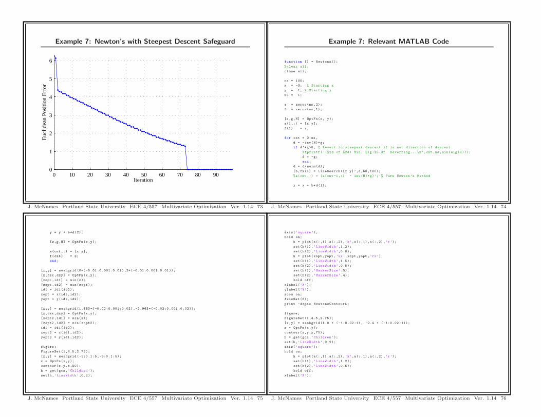
Example 7: Newton’s with Steepest Descent Safeguard
0 0.5 1 1.5 2
−3
−2.5
−2
−1.5
X
Y
J. McNames Portland State University ECE 4/557 Multivariate Optimization Ver. 1.14 71
Newton’s Method
ak+1 = ak − H(ak)−1 ∇f(ak)
where ∇f(ak) is the gradient and H(ak) is the hessian of f(a),
H(ak) ≡
⎡⎢⎢⎢⎢⎢⎣
∂2f(a)∂a2
1
∂2f(a)∂a1 ∂a2
. . . ∂2f(a)∂a1 ∂ap
∂2f(a)∂a2 ∂a1
∂2f(a)∂a2
2. . . ∂2f(a)
∂a2 ∂ap
......
. . ....
∂2f(a)∂ap ∂a1
∂2f(a)∂ap ∂a2
. . . ∂2f(a)∂a2
p
⎤⎥⎥⎥⎥⎥⎦
• Based on a quadratic approximation of the function f(a)
• If f(a) is quadratic, converges in one step
• If H(a) is positive-definite, the problem is well defined near localminima where f(a) is nearly quadratic
J. McNames Portland State University ECE 4/557 Multivariate Optimization Ver. 1.14 69
Example 7: Newton’s with Steepest Descent Safeguard
0 10 20 30 40 50 60 70 80 900
1
2
3
4
5
6
7
Iteration
Func
tion
Val
ue
J. McNames Portland State University ECE 4/557 Multivariate Optimization Ver. 1.14 72
Example 7: Newton’s with Steepest Descent Safeguard
−5 0 5−5
−4
−3
−2
−1
0
1
2
3
4
5
X
Y
J. McNames Portland State University ECE 4/557 Multivariate Optimization Ver. 1.14 70
y = y + b*d(2);
[z,g,H] = OptFn(x,y);
a(cnt ,:) = [x y];
f(cnt) = z;
end;
[x,y] = meshgrid (0+( -0 .01:0.001:0.01),3+(-0.01:0 .001:0.01 ));
[z,dzx ,dzy] = OptFn(x,y);
[zopt ,id1] = min(z);
[zopt ,id2] = min(zopt);
id1 = id1(id2);
xopt = x(id1 ,id2);
yopt = y(id1 ,id2);
[x,y] = meshgrid (1 .883+(-0.02:0.001:0.02),-2.963+(-0.02:0.001:0.02 ));
[z,dzx ,dzy] = OptFn(x,y);
[zopt2 ,id1] = min(z);
[zopt2 ,id2] = min(zopt2);
id1 = id1(id2);
xopt2 = x(id1 ,id2);
yopt2 = y(id1 ,id2);
figure;
FigureSet (1,4.5 ,2.75);
[x,y] = meshgrid (-5:0.1:5,-5:0.1 :5);
z = OptFn(x,y);
contour(x,y,z ,50);
h = get(gca ,’Children ’);
set(h,’LineWidth ’,0.2);
J. McNames Portland State University ECE 4/557 Multivariate Optimization Ver. 1.14 75
Example 7: Newton’s with Steepest Descent Safeguard
0 10 20 30 40 50 60 70 80 900
1
2
3
4
5
6
Iteration
Euc
lidea
n Po
sitio
n E
rror
J. McNames Portland State University ECE 4/557 Multivariate Optimization Ver. 1.14 73
axis(’square’);
hold on;
h = plot(a(:,1),a(:,2),’k’,a(:,1),a(:,2),’r’);
set(h(1),’LineWidth ’,1.2);
set(h(2),’LineWidth ’,0.6);
h = plot(xopt ,yopt ,’kx’,xopt ,yopt ,’rx’);
set(h(1),’LineWidth ’,1.5);
set(h(2),’LineWidth ’,0.5);
set(h(1),’MarkerSize ’ ,5);
set(h(2),’MarkerSize ’ ,4);
hold off;
xlabel(’X’);
ylabel(’Y’);
zoom on;
AxisSet (8);
print -depsc NewtonsContourA;
figure;
FigureSet (1,4.5 ,2.75);
[x,y] = meshgrid (1.0 + (-1:0.02:1), -2.4 + (-1:0.02 :1));
z = OptFn(x,y);
contour(x,y,z ,75);
h = get(gca ,’Children ’);
set(h,’LineWidth ’,0.2);
axis(’square’);
hold on;
h = plot(a(:,1),a(:,2),’k’,a(:,1),a(:,2),’r’);
set(h(1),’LineWidth ’,1.2);
set(h(2),’LineWidth ’,0.6);
hold off;
xlabel(’X’);
J. McNames Portland State University ECE 4/557 Multivariate Optimization Ver. 1.14 76
Example 7: Relevant MATLAB Code
function [] = Newtons ();
%clear all;
close all;
ns = 100;
x = -3; % Starting x
y = 1; % Starting y
b0 = 1;
a = zeros(ns ,2);
f = zeros(ns ,1);
[z,g,H] = OptFn(x, y);
a(1,:) = [x y];
f(1) = z;
for cnt = 2:ns,
d = -inv(H)*g;
if d’*g>0, % Revert to steepest descent if is not direction of descent
%fprintf (’(%2d of %2d) Min. Eig :%5 .3f Reverting...\n’,cnt ,ns,min(eig(H)));
d = -g;
end;
d = d/norm(d);
[b,fmin] = LineSearch ([x y]’,d,b0 ,100);
%a(cnt ,:) = (a(cnt -1,:)’ - inv(H)*g)’; % Pure Newton ’s Method
x = x + b*d(1);
J. McNames Portland State University ECE 4/557 Multivariate Optimization Ver. 1.14 74
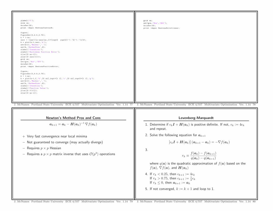
Newton’s Method Pros and Cons
ak+1 = ak − H(ak)−1 ∇f(ak)
+ Very fast convergence near local minima
− Not guaranteed to converge (may actually diverge)
− Requires p × p Hessian
− Requires a p × p matrix inverse that uses O(p3) operations
J. McNames Portland State University ECE 4/557 Multivariate Optimization Ver. 1.14 79
ylabel(’Y’);
zoom on;
AxisSet (8);
print -depsc NewtonsContourB;
figure;
FigureSet (2,4.5 ,2.75);
k = 1:ns;
xerr = (sum (((a-ones(ns ,1)*[ xopt2 yopt2])’).^2)’).^(1/2);
h = plot(k-1,xerr ,’b’);
set(h(1),’Marker’,’.’);
set(h,’MarkerSize ’ ,6);
xlabel(’Iteration ’);
ylabel(’Euclidean Position Error’);
xlim ([0 ns -1]);
ylim ([0 xerr (1)]);
grid on;
set(gca ,’Box’,’Off’);
AxisSet (8);
print -depsc NewtonsPositionError;
figure;
FigureSet (2,4.5 ,2.75);
k = 1:ns;
h = plot(k-1,f,’b’ ,[0 ns],zopt *[1 1],’r’ ,[0 ns],zopt2 *[1 1],’g’);
set(h(1),’Marker’,’.’);
set(h,’MarkerSize ’ ,6);
xlabel(’Iteration ’);
ylabel(’Function Value’);
ylim ([0 f(1)]);
xlim ([0 ns -1]);
J. McNames Portland State University ECE 4/557 Multivariate Optimization Ver. 1.14 77
Levenberg-Marquardt
1. Determine if εkI + H(ak) is positive definite. If not, εk := 4εk
and repeat.
2. Solve the following equation for ak+1
[εkI + H(ak)] (ak+1 − ak) = −∇f(ak)
3.
rk ≡ f(ak) − f(ak+1)q(ak) − q(ak+1)
where q(a) is the quadratic approximation of f(a) based on thef(a), ∇f(a), and H(ak)
4. If rk < 0.25, then εk+1 := 4εk
If rk > 0.75, then εk+1 := 12εk
If rk ≤ 0, then ak+1 := ak
5. If not converged, k := k + 1 and loop to 1.
J. McNames Portland State University ECE 4/557 Multivariate Optimization Ver. 1.14 80
grid on;
set(gca ,’Box’,’Off’);
AxisSet (8);
print -depsc NewtonsErrorLinear;
J. McNames Portland State University ECE 4/557 Multivariate Optimization Ver. 1.14 78
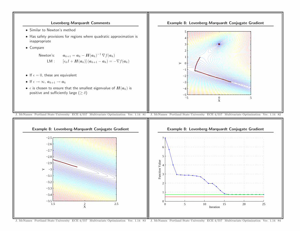
Example 8: Levenberg-Marquardt Conjugate Gradient
1.5 2 2.5−3.5
−3.4
−3.3
−3.2
−3.1
−3
−2.9
−2.8
−2.7
−2.6
−2.5
X
Y
J. McNames Portland State University ECE 4/557 Multivariate Optimization Ver. 1.14 83
Levenberg-Marquardt Comments
• Similar to Newton’s method
• Has safety provisions for regions where quadratic approximation isinappropriate
• Compare
Newton’s: ak+1 = ak − H(ak)−1 ∇f(ak)LM : [εkI + H(ak)] (ak+1 − ak) = −∇f(ak)
• If ε = 0, these are equivalent
• If ε → ∞, ak+1 → ak
• ε is chosen to ensure that the smallest eigenvalue of H(ak) ispositive and sufficiently large (≥ δ)
J. McNames Portland State University ECE 4/557 Multivariate Optimization Ver. 1.14 81
Example 8: Levenberg-Marquardt Conjugate Gradient
0 5 10 15 20 250
1
2
3
4
5
6
7
Iteration
Func
tion
Val
ue
J. McNames Portland State University ECE 4/557 Multivariate Optimization Ver. 1.14 84
Example 8: Levenberg-Marquardt Conjugate Gradient
−5 0 5−5
−4
−3
−2
−1
0
1
2
3
4
5
X
Y
J. McNames Portland State University ECE 4/557 Multivariate Optimization Ver. 1.14 82

y = a(cnt ,2);
zo = zn; % Old function value
zn = OptFn(x,y);
xd = (a(cnt ,:)’-ap);
qo = zo;
qn = zn + g’*xd + 0.5*xd ’*H*xd;
if qo==qn , % Test for convergence
x = a(cnt ,1);
y = a(cnt ,2);
a(cnt:ns ,:) = ones(ns -cnt +1 ,1)*[x y];
f(cnt:ns ,:) = OptFn(x,y);
break;
end;
r = (zo -zn)/(qo-qn);
if r<0.25 ,
eta = eta * 4;
elseif r>0.50 , % 0.75 is recommended , but much slower
eta = eta / 2;
end;
if zn>zo , % Back up
a(cnt ,:) = a(cnt -1 ,:);
else
ap = a(cnt ,:)’;
end;
x = a(cnt ,1);
J. McNames Portland State University ECE 4/557 Multivariate Optimization Ver. 1.14 87
Example 8: Levenberg-Marquardt Conjugate Gradient
0 5 10 15 20 250
1
2
3
4
5
6
Iteration
Euc
lidea
n Po
sitio
n E
rror
J. McNames Portland State University ECE 4/557 Multivariate Optimization Ver. 1.14 85
y = a(cnt ,2);
a(cnt ,:) = [x y];
f(cnt) = OptFn(x,y);
%disp([cnt a(cnt ,:) f(cnt) r eta])
end;
[x,y] = meshgrid (0+( -0 .01:0.001:0.01),3+(-0.01:0 .001:0.01 ));
[z,dzx ,dzy] = OptFn(x,y);
[zopt ,id1] = min(z);
[zopt ,id2] = min(zopt);
id1 = id1(id2);
xopt = x(id1 ,id2);
yopt = y(id1 ,id2);
[x,y] = meshgrid (1 .883+(-0.02:0.001:0.02),-2.963+(-0.02:0.001:0.02 ));
[z,dzx ,dzy] = OptFn(x,y);
[zopt2 ,id1] = min(z);
[zopt2 ,id2] = min(zopt2);
id1 = id1(id2);
xopt2 = x(id1 ,id2);
yopt2 = y(id1 ,id2);
figure;
FigureSet (1,4.5 ,2.75);
[x,y] = meshgrid (-5:0.1:5,-5:0.1 :5);
z = OptFn(x,y);
contour(x,y,z ,50);
h = get(gca ,’Children ’);
set(h,’LineWidth ’,0.2);
axis(’square’);
J. McNames Portland State University ECE 4/557 Multivariate Optimization Ver. 1.14 88
Example 8: Relevant MATLAB Code
function [] = LevenbergMarquardt ();
%clear all;
close all;
ns = 26;
x = -3; % Starting x
y = 1; % Starting y
eta = 0.0001;
a = zeros(ns ,2);
f = zeros(ns ,1);
[zn,g,H] = OptFn(x, y);
a(1,:) = [x y];
f(1) = zn;
ap = [x y]’; % Previous point
for cnt = 2:ns,
[zn ,g,H] = OptFn(x,y);
while min(eig(eta*eye (2)+H))<0,
eta = eta * 4;
end;
a(cnt ,:) = (ap - inv(eta*eye (2)+H)*g )’;
x = a(cnt ,1);
J. McNames Portland State University ECE 4/557 Multivariate Optimization Ver. 1.14 86

set(gca ,’Box’,’Off’);
AxisSet (8);
print -depsc LevenbergMarquardtErrorLinear;
J. McNames Portland State University ECE 4/557 Multivariate Optimization Ver. 1.14 91
hold on;
h = plot(a(:,1),a(:,2),’k’,a(:,1),a(:,2),’r’);
set(h(1),’LineWidth ’,1.2);
set(h(2),’LineWidth ’,0.6);
h = plot(xopt ,yopt ,’kx’,xopt ,yopt ,’rx’);
set(h(1),’LineWidth ’,1.5);
set(h(2),’LineWidth ’,0.5);
set(h(1),’MarkerSize ’ ,5);
set(h(2),’MarkerSize ’ ,4);
hold off;
xlabel(’X’);
ylabel(’Y’);
zoom on;
AxisSet (8);
print -depsc LevenbergMarquardtContourA ;
figure;
FigureSet (1,4.5 ,2.75);
[x,y] = meshgrid (1.5:0.01:2.5 ,-3.5:0.01:-2.5);
z = OptFn(x,y);
contour(x,y,z ,75);
h = get(gca ,’Children ’);
set(h,’LineWidth ’,0.2);
axis(’square’);
hold on;
h = plot(a(:,1),a(:,2),’k’,a(:,1),a(:,2),’r’);
set(h(1),’LineWidth ’,1.2);
set(h(2),’LineWidth ’,0.6);
hold off;
xlabel(’X’);
ylabel(’Y’);
J. McNames Portland State University ECE 4/557 Multivariate Optimization Ver. 1.14 89
Levenberg-Marquardt Pros and Cons
[εkI + H(ak)] (ak+1 − ak) = −∇f(ak)
• Many equivalent formulations
+ No line search required
+ Can be used with approximations to the hessian
+ Extremely fast convergence (2nd order)
− Requires gradient and hessian (or approximate hessian)
− Requires O(p3) operations for each solution to the key equation
J. McNames Portland State University ECE 4/557 Multivariate Optimization Ver. 1.14 92
zoom on;
AxisSet (8);
print -depsc LevenbergMarquardtContourB ;
figure;
FigureSet (2,4.5 ,2.75);
k = 1:ns;
xerr = (sum (((a-ones(ns ,1)*[ xopt2 yopt2])’).^2)’).^(1/2);
h = plot(k-1,xerr ,’b’);
set(h(1),’Marker’,’.’);
set(h,’MarkerSize ’ ,6);
xlabel(’Iteration ’);
ylabel(’Euclidean Position Error’);
xlim ([0 ns -1]);
ylim ([0 xerr (1)]);
grid on;
set(gca ,’Box’,’Off’);
AxisSet (8);
print -depsc LevenbergMarquardtPositionError;
figure;
FigureSet (2,4.5 ,2.75);
k = 1:ns;
h = plot(k-1,f,’b’ ,[0 ns],zopt *[1 1],’r’ ,[0 ns],zopt2 *[1 1],’g’);
set(h(1),’Marker’,’.’);
set(h,’MarkerSize ’ ,6);
xlabel(’Iteration ’);
ylabel(’Function Value’);
ylim ([0 f(1)]);
xlim ([0 ns -1]);
grid on;
J. McNames Portland State University ECE 4/557 Multivariate Optimization Ver. 1.14 90

Optimization Algorithm Summary
Algorithm Convergence Stable ∇f(a) H(a) LSCyclic Coordinate Slow Y N N YSteepest Descent Slow Y Y N YConjugate Gradient Fast N Y N YPARTAN Fast Y Y N YNewton’s Method Very Fast N Y Y NLevenberg-Marquardt Very Fast Y Y Y N
J. McNames Portland State University ECE 4/557 Multivariate Optimization Ver. 1.14 93