Embed Size (px)
Citation preview

Multivariate Statistics
Old School
Mathematical and methodological introduction to multivariate statisticalanalytics, including linear models, principal components, covariance
structures, classification, and clustering, providing background for machinelearning and big data study, with R
John I. Marden
Department of Statistics
University of Illinois at Urbana-Champaign

© 2015 by John I. Marden
Email: [email protected]
URL: http://stat.istics.net/Multivariate
Typeset using the memoir package [Madsen and Wilson, 2015] with LATEX [LaTeXProject Team, 2015]. The faces in the cover image were created using the faces routinein the R package aplpack [Wolf, 2014].

Preface
This text was developed over many years while teaching the graduate course in mul-tivariate analysis in the Department of Statistics, University of Illinois at Urbana-Champaign. Its goal is to teach the basic mathematical grounding that Ph. D. stu-dents need for future research, as well as cover the important multivariate techniquesuseful to statisticians in general.
There is heavy emphasis on multivariate normal modeling and inference, both the-ory and implementation. Several chapters are devoted to developing linear models,including multivariate regression and analysis of variance, and especially the “both-sides models” (i.e., generalized multivariate analysis of variance models), which al-low modeling relationships among variables as well as individuals. Growth curveand repeated measure models are special cases.
Inference on covariance matrices covers testing equality of several covariance ma-trices, testing independence and conditional independence of (blocks of) variables,factor analysis, and some symmetry models. Principal components is a useful graph-ical/exploratory technique, but also lends itself to some modeling.
Classification and clustering are related areas. Both attempt to categorize indi-viduals. Classification tries to classify individuals based upon a previous sample ofobserved individuals and their categories. In clustering, there is no observed catego-rization, nor often even knowledge of how many categories there are. These must beestimated from the data.
Other useful multivariate techniques include biplots, multidimensional scaling,and canonical correlations.
The bulk of the results here are mathematically justified, but I have tried to arrangethe material so that the reader can learn the basic concepts and techniques whileplunging as much or as little as desired into the details of the proofs. Topic- andlevel-wise, this book is somewhere in the convex hull of the classic book by Anderson[2003] and the texts by Mardia, Kent, and Bibby [1979] and Johnson and Wichern[2007], probably closest in spirit to Mardia, Kent and Bibby.
The material assumes the reader has had mathematics up through calculus andlinear algebra, and statistics up through mathematical statistics, e.g., Hogg, McKean,and Craig [2012], and linear regression and analysis of variance, e.g., Weisberg [2013].
In a typical semester, I would cover Chapter 1 (introduction, some graphics, andprincipal components); go through Chapter 2 fairly quickly, as it is a review of mathe-matical statistics the students should know, but being sure to emphasize Section 2.3.1on means and covariance matrices for vectors and matrices, and Section 2.5 on condi-
iii

iv Preface
tional probabilities; go carefully through Chapter 3 on the multivariate normal, andChapter 4 on setting up linear models, including the both-sides model; cover mostof Chapter 5 on projections and least squares, though usually skipping 5.7.1 on theproofs of the QR and Cholesky decompositions; cover Chapters 6 and 7 on estimationand testing in the both-sides model; skip most of Chapter 8, which has many technicalproofs, whose results are often referred to later; cover most of Chapter 9, but usu-ally skip the exact likelihood ratio test in a special case (Section 9.4.1), and Sections9.5.2 and 9.5.3 with details about the Akaike information criterion; cover Chapters10 (covariance models), 11 (classifications), and 12 (clustering) fairly thoroughly; andmake selections from Chapter 13, which presents more on principal components, andintroduces singular value decompositions, multidimensional scaling, and canonicalcorrelations.
A path through the book that emphasizes methodology over mathematical theorywould concentrate on Chapters 1 (skip Section 1.8), 4, 6, 7 (skip Sections 7.2.5 and7.5.2), 9 (skip Sections 9.3.4, 9.5.1. 9.5.2, and 9.5.3), 10 (skip Section 10.4), 11, 12(skip Section 12.4), and 13 (skip Sections 13.1.5 and 13.1.6). The more data-orientedexercises come at the end of each chapter’s set of exercises.
One feature of the text is a fairly rigorous presentation of the basics of linear al-gebra that are useful in statistics. Sections 1.4, 1.5, 1.6, and 1.8 and Exercises 1.9.1through 1.9.13 cover idempotent matrices, orthogonal matrices, and the spectral de-composition theorem for symmetric matrices, including eigenvectors and eigenval-ues. Sections 3.1 and 3.3 and Exercises 3.7.6, 3.7.12, 3.7.16 through 3.7.20, and 3.7.24cover positive and nonnegative definiteness, Kronecker products, and the Moore-Penrose inverse for symmetric matrices. Chapter 5 covers linear subspaces, linearindependence, spans, bases, projections, least squares, Gram-Schmidt orthogonaliza-tion, orthogonal polynomials, and the QR and Cholesky decompositions. Section13.1.3 and Exercise 13.4.3 look further at eigenvalues and eigenspaces, and Section13.3 and Exercise 13.4.12 develop the singular value decomposition.
Practically all the calculations and graphics in the examples are implementedusing the statistical computing environment R [R Development Core Team, 2015].Throughout the text we have scattered some of the actual R code we used. Many ofthe data sets and original R functions can be found in the R package msos [Mardenand Balamuta, 2014], thanks to the much appreciated efforts of James Balamuta. Forother material we refer to available R packages.
I thank Michael Perlman for introducing me to multivariate analysis, and hisfriendship and mentorship throughout my career. Most of the ideas and approachesin this book got their start in the multivariate course I took from him forty years ago.I think they have aged well. Also, thanks to Steen Andersson, from whom I learneda lot, including the idea that one should define a model before trying to analyze it.
This book is dedicated to Ann.

Contents
Preface iii
Contents v
1 A First Look at Multivariate Data 11.1 The data matrix . . . . . . . . . . . . . . . . . . . . . . . . . . . . . . . . . 1
1.1.1 Example: Planets data . . . . . . . . . . . . . . . . . . . . . . . . . 21.2 Glyphs . . . . . . . . . . . . . . . . . . . . . . . . . . . . . . . . . . . . . . 21.3 Scatter plots . . . . . . . . . . . . . . . . . . . . . . . . . . . . . . . . . . . 3
1.3.1 Example: Fisher-Anderson iris data . . . . . . . . . . . . . . . . . 51.4 Sample means, variances, and covariances . . . . . . . . . . . . . . . . . 61.5 Marginals and linear combinations . . . . . . . . . . . . . . . . . . . . . . 8
1.5.1 Rotations . . . . . . . . . . . . . . . . . . . . . . . . . . . . . . . . 101.6 Principal components . . . . . . . . . . . . . . . . . . . . . . . . . . . . . 10
1.6.1 Biplots . . . . . . . . . . . . . . . . . . . . . . . . . . . . . . . . . . 131.6.2 Example: Sports data . . . . . . . . . . . . . . . . . . . . . . . . . 13
1.7 Other projections to pursue . . . . . . . . . . . . . . . . . . . . . . . . . . 151.7.1 Example: Iris data . . . . . . . . . . . . . . . . . . . . . . . . . . . 17
1.8 Proofs . . . . . . . . . . . . . . . . . . . . . . . . . . . . . . . . . . . . . . . 181.9 Exercises . . . . . . . . . . . . . . . . . . . . . . . . . . . . . . . . . . . . . 20
2 Multivariate Distributions 272.1 Probability distributions . . . . . . . . . . . . . . . . . . . . . . . . . . . . 27
2.1.1 Distribution functions . . . . . . . . . . . . . . . . . . . . . . . . . 272.1.2 Densities . . . . . . . . . . . . . . . . . . . . . . . . . . . . . . . . 282.1.3 Representations . . . . . . . . . . . . . . . . . . . . . . . . . . . . 292.1.4 Conditional distributions . . . . . . . . . . . . . . . . . . . . . . . 30
2.2 Expected values . . . . . . . . . . . . . . . . . . . . . . . . . . . . . . . . . 322.3 Means, variances, and covariances . . . . . . . . . . . . . . . . . . . . . . 33
2.3.1 Vectors and matrices . . . . . . . . . . . . . . . . . . . . . . . . . . 342.3.2 Moment generating functions . . . . . . . . . . . . . . . . . . . . 35
2.4 Independence . . . . . . . . . . . . . . . . . . . . . . . . . . . . . . . . . . 352.5 Additional properties of conditional distributions . . . . . . . . . . . . . 372.6 Affine transformations . . . . . . . . . . . . . . . . . . . . . . . . . . . . . 40
v

vi Contents
2.7 Exercises . . . . . . . . . . . . . . . . . . . . . . . . . . . . . . . . . . . . . 41
3 The Multivariate Normal Distribution 493.1 Definition . . . . . . . . . . . . . . . . . . . . . . . . . . . . . . . . . . . . 493.2 Some properties of the multivariate normal . . . . . . . . . . . . . . . . . 513.3 Multivariate normal data matrix . . . . . . . . . . . . . . . . . . . . . . . 523.4 Conditioning in the multivariate normal . . . . . . . . . . . . . . . . . . 553.5 The sample covariance matrix: Wishart distribution . . . . . . . . . . . . 573.6 Some properties of the Wishart . . . . . . . . . . . . . . . . . . . . . . . . 593.7 Exercises . . . . . . . . . . . . . . . . . . . . . . . . . . . . . . . . . . . . . 60
4 Linear Models on Both Sides 694.1 Linear regression . . . . . . . . . . . . . . . . . . . . . . . . . . . . . . . . 694.2 Multivariate regression and analysis of variance . . . . . . . . . . . . . . 72
4.2.1 Examples of multivariate regression . . . . . . . . . . . . . . . . . 724.3 Linear models on both sides . . . . . . . . . . . . . . . . . . . . . . . . . 77
4.3.1 One individual . . . . . . . . . . . . . . . . . . . . . . . . . . . . . 774.3.2 IID observations . . . . . . . . . . . . . . . . . . . . . . . . . . . . 784.3.3 The both-sides model . . . . . . . . . . . . . . . . . . . . . . . . . 81
4.4 Exercises . . . . . . . . . . . . . . . . . . . . . . . . . . . . . . . . . . . . . 82
5 Linear Models: Least Squares and Projections 875.1 Linear subspaces . . . . . . . . . . . . . . . . . . . . . . . . . . . . . . . . 875.2 Projections . . . . . . . . . . . . . . . . . . . . . . . . . . . . . . . . . . . . 895.3 Least squares . . . . . . . . . . . . . . . . . . . . . . . . . . . . . . . . . . 905.4 Best linear unbiased estimators . . . . . . . . . . . . . . . . . . . . . . . . 915.5 Least squares in the both-sides model . . . . . . . . . . . . . . . . . . . . 935.6 What is a linear model? . . . . . . . . . . . . . . . . . . . . . . . . . . . . 945.7 Gram-Schmidt orthogonalization . . . . . . . . . . . . . . . . . . . . . . . 95
5.7.1 The QR and Cholesky decompositions . . . . . . . . . . . . . . . 975.7.2 Orthogonal polynomials . . . . . . . . . . . . . . . . . . . . . . . 99
5.8 Exercises . . . . . . . . . . . . . . . . . . . . . . . . . . . . . . . . . . . . . 101
6 Both-Sides Models: Estimation 1096.1 Distribution of β . . . . . . . . . . . . . . . . . . . . . . . . . . . . . . . . 1096.2 Estimating the covariance . . . . . . . . . . . . . . . . . . . . . . . . . . . 109
6.2.1 Multivariate regression . . . . . . . . . . . . . . . . . . . . . . . . 1096.2.2 Both-sides model . . . . . . . . . . . . . . . . . . . . . . . . . . . . 111
6.3 Standard errors and t-statistics . . . . . . . . . . . . . . . . . . . . . . . . 1116.4 Examples . . . . . . . . . . . . . . . . . . . . . . . . . . . . . . . . . . . . . 112
6.4.1 Mouth sizes . . . . . . . . . . . . . . . . . . . . . . . . . . . . . . . 1126.4.2 Using linear regression routines . . . . . . . . . . . . . . . . . . . 1146.4.3 Leprosy data . . . . . . . . . . . . . . . . . . . . . . . . . . . . . . 1156.4.4 Covariates: Leprosy data . . . . . . . . . . . . . . . . . . . . . . . 1156.4.5 Histamine in dogs . . . . . . . . . . . . . . . . . . . . . . . . . . . 117
6.5 Submodels of the both-sides model . . . . . . . . . . . . . . . . . . . . . 1186.6 Exercises . . . . . . . . . . . . . . . . . . . . . . . . . . . . . . . . . . . . . 120
7 Both-Sides Models: Hypothesis Tests on β 1257.1 Approximate χ2 test . . . . . . . . . . . . . . . . . . . . . . . . . . . . . . 125

Contents vii
7.1.1 Example: Mouth sizes . . . . . . . . . . . . . . . . . . . . . . . . . 1267.2 Testing blocks of β are zero . . . . . . . . . . . . . . . . . . . . . . . . . . 126
7.2.1 Just one column: F test . . . . . . . . . . . . . . . . . . . . . . . . 1287.2.2 Just one row: Hotelling’s T2 . . . . . . . . . . . . . . . . . . . . . 1287.2.3 General blocks . . . . . . . . . . . . . . . . . . . . . . . . . . . . . 1297.2.4 Additional test statistics . . . . . . . . . . . . . . . . . . . . . . . . 1297.2.5 The between and within matrices . . . . . . . . . . . . . . . . . . 130
7.3 Examples . . . . . . . . . . . . . . . . . . . . . . . . . . . . . . . . . . . . . 1327.3.1 Mouth sizes . . . . . . . . . . . . . . . . . . . . . . . . . . . . . . . 1327.3.2 Histamine in dogs . . . . . . . . . . . . . . . . . . . . . . . . . . . 133
7.4 Testing linear restrictions . . . . . . . . . . . . . . . . . . . . . . . . . . . 1347.5 Model selection: Mallows’ Cp . . . . . . . . . . . . . . . . . . . . . . . . . 135
7.5.1 Example: Mouth sizes . . . . . . . . . . . . . . . . . . . . . . . . . 1377.5.2 Mallows’ Cp verification . . . . . . . . . . . . . . . . . . . . . . . 139
7.6 Exercises . . . . . . . . . . . . . . . . . . . . . . . . . . . . . . . . . . . . . 141
8 Some Technical Results 1458.1 The Cauchy-Schwarz inequality . . . . . . . . . . . . . . . . . . . . . . . 1458.2 Conditioning in a Wishart . . . . . . . . . . . . . . . . . . . . . . . . . . . 1468.3 Expected value of the inverse Wishart . . . . . . . . . . . . . . . . . . . . 147
8.4 Distribution of Hotelling’s T2 . . . . . . . . . . . . . . . . . . . . . . . . . 148
8.4.1 A motivation for Hotelling’s T2 . . . . . . . . . . . . . . . . . . . 1498.5 Density of the multivariate normal . . . . . . . . . . . . . . . . . . . . . . 1508.6 The QR decomposition for the multivariate normal . . . . . . . . . . . . 1518.7 Density of the Wishart . . . . . . . . . . . . . . . . . . . . . . . . . . . . . 1538.8 Exercises . . . . . . . . . . . . . . . . . . . . . . . . . . . . . . . . . . . . . 154
9 Likelihood Methods 1619.1 Likelihood . . . . . . . . . . . . . . . . . . . . . . . . . . . . . . . . . . . . 1619.2 Maximum likelihood estimation . . . . . . . . . . . . . . . . . . . . . . . 1619.3 The MLE in the both-sides model . . . . . . . . . . . . . . . . . . . . . . 162
9.3.1 Maximizing the likelihood . . . . . . . . . . . . . . . . . . . . . . 1629.3.2 Examples . . . . . . . . . . . . . . . . . . . . . . . . . . . . . . . . 1649.3.3 Calculating the estimates . . . . . . . . . . . . . . . . . . . . . . . 1669.3.4 Proof of the MLE for the Wishart . . . . . . . . . . . . . . . . . . 168
9.4 Likelihood ratio tests . . . . . . . . . . . . . . . . . . . . . . . . . . . . . . 1689.4.1 The LRT in the both-sides model . . . . . . . . . . . . . . . . . . 169
9.5 Model selection: AIC and BIC . . . . . . . . . . . . . . . . . . . . . . . . 1709.5.1 BIC: Motivation . . . . . . . . . . . . . . . . . . . . . . . . . . . . 1719.5.2 AIC: Motivation . . . . . . . . . . . . . . . . . . . . . . . . . . . . 1739.5.3 AIC: Multivariate regression . . . . . . . . . . . . . . . . . . . . . 1749.5.4 Example: Skulls . . . . . . . . . . . . . . . . . . . . . . . . . . . . 1759.5.5 Example: Histamine . . . . . . . . . . . . . . . . . . . . . . . . . . 179
9.6 Exercises . . . . . . . . . . . . . . . . . . . . . . . . . . . . . . . . . . . . . 181
10 Models on Covariance Matrices 18710.1 Testing equality of covariance matrices . . . . . . . . . . . . . . . . . . . 188
10.1.1 Example: Grades data . . . . . . . . . . . . . . . . . . . . . . . . . 18910.1.2 Testing the equality of several covariance matrices . . . . . . . . 190
10.2 Testing independence of two blocks of variables . . . . . . . . . . . . . . 190

viii Contents
10.2.1 Example: Grades data . . . . . . . . . . . . . . . . . . . . . . . . . 19110.2.2 Example: Testing conditional independence . . . . . . . . . . . . 192
10.3 Factor analysis . . . . . . . . . . . . . . . . . . . . . . . . . . . . . . . . . 19410.3.1 Estimation . . . . . . . . . . . . . . . . . . . . . . . . . . . . . . . . 19510.3.2 Describing the factors . . . . . . . . . . . . . . . . . . . . . . . . . 19710.3.3 Example: Grades data . . . . . . . . . . . . . . . . . . . . . . . . . 198
10.4 Some symmetry models . . . . . . . . . . . . . . . . . . . . . . . . . . . . 20210.4.1 Some types of symmetry . . . . . . . . . . . . . . . . . . . . . . . 20310.4.2 Characterizing the structure . . . . . . . . . . . . . . . . . . . . . 20510.4.3 Maximum likelihood estimates . . . . . . . . . . . . . . . . . . . 20510.4.4 Hypothesis testing and model selection . . . . . . . . . . . . . . 20710.4.5 Example: Mouth sizes . . . . . . . . . . . . . . . . . . . . . . . . . 207
10.5 Exercises . . . . . . . . . . . . . . . . . . . . . . . . . . . . . . . . . . . . . 210
11 Classification 21511.1 Mixture models . . . . . . . . . . . . . . . . . . . . . . . . . . . . . . . . . 21511.2 Classifiers . . . . . . . . . . . . . . . . . . . . . . . . . . . . . . . . . . . . 21711.3 Fisher’s linear discrimination . . . . . . . . . . . . . . . . . . . . . . . . . 21911.4 Cross-validation estimate of error . . . . . . . . . . . . . . . . . . . . . . 221
11.4.1 Example: Iris data . . . . . . . . . . . . . . . . . . . . . . . . . . . 22211.5 Fisher’s quadratic discrimination . . . . . . . . . . . . . . . . . . . . . . . 225
11.5.1 Example: Iris data, continued . . . . . . . . . . . . . . . . . . . . 22611.6 Modifications to Fisher’s discrimination . . . . . . . . . . . . . . . . . . . 22711.7 Conditioning on X: Logistic regression . . . . . . . . . . . . . . . . . . . 227
11.7.1 Example: Iris data . . . . . . . . . . . . . . . . . . . . . . . . . . . 22911.7.2 Example: Spam . . . . . . . . . . . . . . . . . . . . . . . . . . . . . 230
11.8 Trees . . . . . . . . . . . . . . . . . . . . . . . . . . . . . . . . . . . . . . . 23311.8.1 CART . . . . . . . . . . . . . . . . . . . . . . . . . . . . . . . . . . 235
11.9 Exercises . . . . . . . . . . . . . . . . . . . . . . . . . . . . . . . . . . . . . 240
12 Clustering 24512.1 K-means . . . . . . . . . . . . . . . . . . . . . . . . . . . . . . . . . . . . . 246
12.1.1 Example: Sports data . . . . . . . . . . . . . . . . . . . . . . . . . 24612.1.2 Silhouettes . . . . . . . . . . . . . . . . . . . . . . . . . . . . . . . 24712.1.3 Plotting clusters in one and two dimensions . . . . . . . . . . . . 24812.1.4 Example: Sports data, using R . . . . . . . . . . . . . . . . . . . . 250
12.2 K-medoids . . . . . . . . . . . . . . . . . . . . . . . . . . . . . . . . . . . . 25212.3 Model-based clustering . . . . . . . . . . . . . . . . . . . . . . . . . . . . 254
12.3.1 Example: Automobile data . . . . . . . . . . . . . . . . . . . . . . 25412.3.2 Some of the models in mclust . . . . . . . . . . . . . . . . . . . . 257
12.4 An example of the EM algorithm . . . . . . . . . . . . . . . . . . . . . . . 25912.5 Soft K-means . . . . . . . . . . . . . . . . . . . . . . . . . . . . . . . . . . 260
12.5.1 Example: Sports data . . . . . . . . . . . . . . . . . . . . . . . . . 26112.6 Hierarchical clustering . . . . . . . . . . . . . . . . . . . . . . . . . . . . . 261
12.6.1 Example: Grades data . . . . . . . . . . . . . . . . . . . . . . . . . 26212.6.2 Example: Sports data . . . . . . . . . . . . . . . . . . . . . . . . . 263
12.7 Exercises . . . . . . . . . . . . . . . . . . . . . . . . . . . . . . . . . . . . . 265
13 Principal Components and Related Techniques 26713.1 Principal components, redux . . . . . . . . . . . . . . . . . . . . . . . . . 267
Contents ix
13.1.1 Example: Iris data . . . . . . . . . . . . . . . . . . . . . . . . . . . 26813.1.2 Choosing the number of principal components . . . . . . . . . . 27013.1.3 Estimating the structure of the component spaces . . . . . . . . . 27113.1.4 Example: Automobile data . . . . . . . . . . . . . . . . . . . . . . 27313.1.5 Principal components and factor analysis . . . . . . . . . . . . . 27613.1.6 Justification of the principal component MLE . . . . . . . . . . . 278
13.2 Multidimensional scaling . . . . . . . . . . . . . . . . . . . . . . . . . . . 28013.2.1 ∆ is Euclidean: The classical solution . . . . . . . . . . . . . . . . 28013.2.2 ∆ may not be Euclidean: The classical solution . . . . . . . . . . 28213.2.3 Non-metric approach . . . . . . . . . . . . . . . . . . . . . . . . . 28313.2.4 Examples: Grades and sports . . . . . . . . . . . . . . . . . . . . 283
13.3 Canonical correlations . . . . . . . . . . . . . . . . . . . . . . . . . . . . . 28413.3.1 Example: Grades . . . . . . . . . . . . . . . . . . . . . . . . . . . . 28713.3.2 How many canonical correlations are positive? . . . . . . . . . . 28813.3.3 Partial least squares . . . . . . . . . . . . . . . . . . . . . . . . . . 290
13.4 Exercises . . . . . . . . . . . . . . . . . . . . . . . . . . . . . . . . . . . . . 290
A Extra R Routines 295A.1 Entropy . . . . . . . . . . . . . . . . . . . . . . . . . . . . . . . . . . . . . . 295
A.1.1 negent: Estimate negative entropy . . . . . . . . . . . . . . . . . . 296A.1.2 negent2D: Maximize negentropy for two dimensions . . . . . . . 296A.1.3 negent3D: Maximize negentropy for three dimensions . . . . . . 297
A.2 Both-sides model . . . . . . . . . . . . . . . . . . . . . . . . . . . . . . . . 297A.2.1 bothsidesmodel: Calculate the least squares estimates . . . . . . . 298A.2.2 reverse.kronecker: Reverse the matrices in a Kronecker product . 299A.2.3 bothsidesmodel.mle: Calculate the maximum likelihood estimates 299A.2.4 bothsidesmodel.chisquare: Test subsets of β are zero . . . . . . . . 300A.2.5 bothsidesmodel.hotelling: Test blocks of β are zero . . . . . . . . . 300A.2.6 bothsidesmodel.lrt: Test subsets of β are zero . . . . . . . . . . . . 301A.2.7 Helper functions . . . . . . . . . . . . . . . . . . . . . . . . . . . . 302
A.3 Classification . . . . . . . . . . . . . . . . . . . . . . . . . . . . . . . . . . 302A.3.1 lda: Linear discrimination . . . . . . . . . . . . . . . . . . . . . . . 302A.3.2 qda: Quadratic discrimination . . . . . . . . . . . . . . . . . . . . 302A.3.3 predict_qda: Quadratic discrimination prediction . . . . . . . . . 303
A.4 Silhouettes for K-means clustering . . . . . . . . . . . . . . . . . . . . . . 303A.4.1 silhouette.km: Calculate the silhouettes . . . . . . . . . . . . . . . 303A.4.2 sort_silhouette: Sort the silhouettes by group . . . . . . . . . . . 303
A.5 Patterns of eigenvalues . . . . . . . . . . . . . . . . . . . . . . . . . . . . . 304A.5.1 pcbic: BIC for a particular pattern . . . . . . . . . . . . . . . . . . 304A.5.2 pcbic.stepwise: Choose a good pattern . . . . . . . . . . . . . . . 304A.5.3 Helper functions . . . . . . . . . . . . . . . . . . . . . . . . . . . . 305
A.6 Function listings . . . . . . . . . . . . . . . . . . . . . . . . . . . . . . . . 305
Bibliography 317
Author Index 325
Subject Index 329


Chapter 1
A First Look at Multivariate Data
In this chapter, we try to give a sense of what multivariate data sets look like, andintroduce some of the basic matrix manipulations needed throughout these notes.Chapters 2 and 3 lay down the distributional theory. Linear models are probably themost popular statistical models ever. With multivariate data, we can model relation-ships between individuals or between variables, leading to what we call “both-sidesmodels,” which do both simultaneously. Chapters 4 through 8 present these modelsin detail. The linear models are concerned with means. Before turning to modelson covariances, Chapter 9 briefly reviews likelihood methods, including maximumlikelihood estimation, likelihood ratio tests, and model selection criteria (Bayes andAkaike). Chapter 10 looks at a number of models based on covariance matrices, in-cluding equality of covariances, independence and conditional independence, factoranalysis, and other structural models. Chapter 11 deals with classification, in whichthe goal is to find ways to classify individuals into categories, e.g., healthy or un-healthy, based on a number of observed variable. Chapter 12 has a similar goal,except that the categories are unknown and we seek to group individuals based onjust the observed variables. Finally, Chapter 13 explores principal components, whichwe first see in Section 1.6. It is an approach for reducing the number of variables,or at least find a few interesting ones, by searching through linear combinations ofthe observed variables. Multidimensional scaling has a similar objective, but tries toexhibit the individual data points in a low-dimensional space while preserving theoriginal inter-point distances. Canonical correlations has two sets of variables, andfinds linear combinations of the two sets to explain the correlations between them.
On to the data.
1.1 The data matrix
Data generally will consist of a number of variables recorded on a number of individ-uals, e.g., heights, weights, ages, and sexes of a sample of students. Also, generally,there will be n individuals and q variables, and the data will be arranged in an n × q
1

2 Chapter 1. Multivariate Data
data matrix, with rows denoting individuals and the columns denoting variables:
Y =
Var 1 Var 2 · · · Var qIndividual 1Individual 2
...Individual n
y11 y12 . . . y1q
y21 y22 . . . y2q
......
. . ....
yn1 yn2 . . . ynq
.
(1.1)
Then yij is the value of the variable j for individual i. Much more complex datastructures exist, but this course concentrates on these straightforward data matrices.
1.1.1 Example: Planets data
Six astronomical variables are given on each of the historical nine planets (or eightplanets, plus Pluto). The variables are (average) distance in millions of miles fromthe Sun, length of day in Earth days, length of year in Earth days, diameter in miles,temperature in degrees Fahrenheit, and number of moons. The data matrix:
Dist Day Year Diam Temp MoonsMercury 35.96 59.00 88.00 3030 332 0Venus 67.20 243.00 224.70 7517 854 0Earth 92.90 1.00 365.26 7921 59 1Mars 141.50 1.00 687.00 4215 −67 2Jupiter 483.30 0.41 4332.60 88803 −162 16Saturn 886.70 0.44 10759.20 74520 −208 18Uranus 1782.00 0.70 30685.40 31600 −344 15Neptune 2793.00 0.67 60189.00 30200 −261 8Pluto 3664.00 6.39 90465.00 1423 −355 1
(1.2)
The data can be found in Wright [1997], for example.
1.2 Glyphs
Graphical displays of univariate data, that is, data on one variable, are well-known:histograms, stem-and-leaf plots, pie charts, box plots, etc. For two variables, scat-ter plots are valuable. It is more of a challenge when dealing with three or morevariables.
Glyphs provide an option. A little picture is created for each individual, with char-acteristics based on the values of the variables. Chernoff’s faces [Chernoff, 1973] maybe the most famous glyphs. The idea is that people intuitively respond to character-istics of faces, so that many variables can be summarized in a face.
Figure 1.1 exhibits faces for the nine planets. We use the faces routine by H. P.Wolf in the R package aplpack, Wolf [2014]. The distance the planet is from the sunis represented by the height of the face (Pluto has a long face), the length of theplanet’s day by the width of the face (Venus has a wide face), etc. One can thencluster the planets. Mercury, Earth and Mars look similar, as do Saturn and Jupiter.These face plots are more likely to be amusing than useful, especially if the numberof individuals is large. A star plot is similar. Each individual is represented by aq-pointed star, where each point corresponds to a variable, and the distance of the

1.3. Scatter plots 3
Mercury Venus Earth
Mars Jupiter Saturn
Uranus Neptune Pluto
Figure 1.1: Chernoff’s faces for the planets. Each feature represents a variable. Forthese data, distance = height of face, day = width of face, year = shape of face, diameter =height of mouth, temperature = width of mouth, moons = curve of smile.
point from the center is based on the variable’s value for that individual. See Figure1.2.
1.3 Scatter plots
Two-dimensional scatter plots can be enhanced by using different symbols for theobservations instead of plain dots. For example, different colors could be used fordifferent groups of points, or glyphs representing other variables could be plotted.Figure 1.2 plots the planets with the logarithms of day length and year length as theaxes, where the stars created from the other four variables are the plotted symbols.Note that the planets pair up in a reasonable way. Mercury and Venus are close, bothin terms of the scatter plot and in the look of their stars. Similarly, Earth and Marspair up, as do Jupiter and Saturn, and Uranus and Neptune. See Listing 1.1 for the Rcode.
A scatter plot matrix arranges all possible two-way scatter plots in a q × q matrix.These displays can be enhanced with brushing, in which individual points or groupsof points can be selected in one plot, and be simultaneously highlighted in the otherplots.

4 Chapter 1. Multivariate Data
Listing 1.1: R code for the star plot of the planets, Figure 1.2. The data are in thematrix planets. The first statement normalizes the variables to range from 0 to 1. Theep matrix is used to place the names of the planets. Tweaking is necessary, dependingon the size of the plot.
p <− apply(planets,2,function(z) (z−min(z))/(max(z)−min(z)))x <− log(planets[,2])y <− log(planets[,3])ep <− rbind(c(−.3,.4),c(−.5,.4),c(.5,0),c(.5,0),c(.6,−1),c(−.5,1.4),
c(1,−.6),c(1.3,.4),c(1,−.5))symbols(x,y,stars=p[,−(2:3)],xlab=’log(day)’,ylab=’log(year)’,inches=.4)text(x+ep[,1],y+ep[,2],labels=rownames(planets),cex=.7)
0 2 4 6
46
810
12
Mercury
VenusEarth
Mars
Jupiter
Saturn
Uranus
Neptune
Pluto
log(day)
log(
year
)
Figure 1.2: Scatter plot of log(day) versus log(year) for the planets, with plottingsymbols being stars created from the other four variables: distance, diameter, tem-perature, moons.
1.3. Scatter plots 5
Sepal.Length
sssss
s
ss
ss
sss
s
s ssssss s
ssss ssssss ssssss
sss
s ss ss s
sss
vvv
v
v
vv
v
v
vv
vv vv
v
vvv
v vvv vvvvv
vvvv vvv
vv
vvvvvv
vv vv
v
vv
gg
g
gg
g
g
gg
ggg
g
g ggg
gg
g
g
g
g
gg
g
ggg
ggg
ggg
g
ggg
ggg
g
gggg g gg
ssssss
sssssss
s
ssssssss
ssssssssssssssssssssssssssss
vvv
v
v
vv
v
v
vv
vv vv
v
vvv
v vv vvvvvv
vvvvvv
vvv
vvvv
vv
vvvvv
vv
gg
g
gg
g
g
ggg
ggg
gggg
gg
g
g
g
g
ggg
gg g
ggg
ggg
g
ggg
ggg
g
ggggggg
sssss
s
ssssssss
ssssssss
sssssss
sssssss
sssssss
sssssss
vvv
v
v
vv
v
v
vv
vv vv
v
vvv
v vvvvvvv vvvvvv vvvv
vvvvvv
vvvvv
vv
gg
g
g g
g
g
gg
gggg
g ggg
gg
g
g
g
g
gg
g
gg g
g gg
ggg
g
ggg
g gg
g
ggggg gg
sssss
ss s
s s
ssss
ss
ss
sss
ssssssssss
s
ss
ssss
sss
s
sss
s
s
ss
s vv v
vvv
v
vvv
v
v
v
vv vvv
vv
vvv
vvvvvvvvvvv
vv
v
v
vvv
vv
vvvv v
vv
g
gggg g
gg
g
ggg
ggg
gg
g
gg
gg gg
g gggg gg
g
gggg
ggg ggg
gggg
gg
gg Sepal.Width
ssssss
ssss
ssss
ssssssssssssssssss
ss
ssss
sss
s
sss
s
s
sss vvv
vvvv
vvv
v
v
v
vv vvvv
v
vv
vvvvvvv
vvvv v
vvv
v
vvv
vv
vvvvv
vv
g
gggg g
gg
g
gggg
gggg
g
gg
gg gg
gggg ggg
g
gggg
gggggg
gggg
ggg
gsssss
sss
ss
ssss
sss
sss
sssss
sssssss
ss
ssss
sss
s
ss
s
s
s
sss vvv
vvvv
vvv
v
v
v
vvvvvv
v
vv
vvvvv vv
vvvv v
vvv
v
vvvv
vv
vvvv
vv
g
ggg gg
ggg
ggg
gg
ggg
g
gg
gggg
gggg gg g
g
ggggg
gg g ggg
ggg
gg
gg
ssss s ss ss s ssss ssss sssssssssssss sssss sss ssss sssss ss
vv vv
vv v
v
vvv
vvv
vvvv v
vvvvvvvv
vvvvvv
vv v vvvvv
vv
vvvv v
vv
gg
gggg
g
gg ggg ggg gg
gg
gg
g
g
gg g
ggg gg
gggg
gggg
ggggggggggg
ssss s sssss ssss s sss sss sssss sssss s ssss sss sss s s ss ss ss
vvvvvv v
v
vvv
vvvv
vvvvv
vv
v vvvvvvvvv vv
v vvv vvvv
vv
v vvv
vv
gg
gggg
g
gg ggg gg g gg
gg
gg
g
g
ggg
ggggg gggg g gg
ggggggggg g gg
Petal.Length
sssssssssssssssssssssssssssssssssssssssssss sssssss
vvvvvv v
v
vvvvv
vvvvv v
vv
vvvvvv
vvvvvv
vvvvvvvv
vv
vvvvv
vv
gg
gg gg
g
gg ggggg ggg
gg
gg
g
g
ggg
gggg ggggg
gggg
g gggggggg gg
ssss s ss ss s ssss ssss ssssss
sssssss sssss sss ssss
sssss ss
vv vv vvv
vvv
vvvvv vv
vv
v
vvvvvvv
vvvvvv
vv v vvvvv vvvvvv vv v
g
g ggg g
g gg
ggg gg
g gg
gg
g
gg gg
gggg
ggg gg
gg
gg
ggg
ggg
gggggg
g
ssss s sssss ssss s sss sss sssss sssss s
ssss sss sss ss ss ss ss
vvvv vvv
vvv
vv
vvvvv
vv
v
vvvvvvv
vvvvv vv v vvv vvv vvvv vvvv v
g
g gggg
g gg
ggg gg
g gg
gg
g
gggg
gggg
gg
g gg
gg
g g
ggggg
gggg
g gg
g
sssssssssssssssssssssssssssssssssssssssssss
sssssss
vvvv vvv
vvv
vvv
vv vvvv
v
vv v
vvvvvv
vvvvvvvvvvvvvvv
vvvvv v
g
g ggg g
g gg
gggggggg
gg
g
gg gg
gggg
gggg
g
gg
gg
ggggg
gggg
ggg
g
Petal.Width
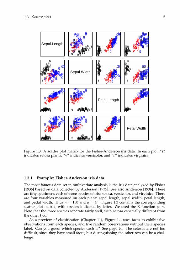
Figure 1.3: A scatter plot matrix for the Fisher-Anderson iris data. In each plot, “s”indicates setosa plants, “v” indicates versicolor, and “r” indicates virginica.
1.3.1 Example: Fisher-Anderson iris data
The most famous data set in multivariate analysis is the iris data analyzed by Fisher[1936] based on data collected by Anderson [1935]. See also Anderson [1936]. Thereare fifty specimens each of three species of iris: setosa, versicolor, and virginica. Thereare four variables measured on each plant: sepal length, sepal width, petal length,and pedal width. Thus n = 150 and q = 4. Figure 1.3 contains the correspondingscatter plot matrix, with species indicated by letter. We used the R function pairs.Note that the three species separate fairly well, with setosa especially different fromthe other two.
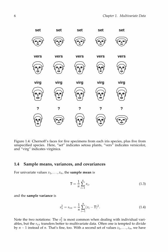
As a preview of classification (Chapter 11), Figure 1.4 uses faces to exhibit fiveobservations from each species, and five random observations without their specieslabel. Can you guess which species each is? See page 20. The setosas are not toodifficult, since they have small faces, but distinguishing the other two can be a chal-lenge.
6 Chapter 1. Multivariate Data
set set set set set
vers vers vers vers vers
virg virg virg virg virg
? ? ? ? ?
Figure 1.4: Chernoff’s faces for five specimens from each iris species, plus five fromunspecified species. Here, “set” indicates setosa plants, “vers” indicates versicolor,and “virg” indicates virginica.
1.4 Sample means, variances, and covariances
For univariate values x1, . . . , xn, the sample mean is
x =1
n
n
∑i=1
xi, (1.3)
and the sample variance is
s2x = sxx =
1
n
n
∑i=1
(xi − x)2. (1.4)
Note the two notations: The s2x is most common when dealing with individual vari-
ables, but the sxx transfers better to multivariate data. Often one is tempted to divideby n − 1 instead of n. That’s fine, too. With a second set of values z1, . . . , zn, we have

1.4. Sample means, variances, and covariances 7
the sample covariance between the xi’s and zi’s to be
sxz =1
n
n
∑i=1
(xi − x)(zi − z). (1.5)
So the covariance between the xi’s and themselves is the variance, which is to say that
s2x = sxx. The sample correlation coefficient is a normalization of the covariance that
ranges between −1 and +1, defined by
rxz =sxz
sxsz(1.6)
provided both variances are positive. (See Corollary 8.1.) In a scatter plot of x versusz, the correlation coefficient is +1 if all the points lie on a line with positive slope,and −1 if they all lie on a line with negative slope.
For a data matrix Y (1.1) with q variables, there are q means:
yj =1
n
n
∑i=1
yij. (1.7)
Placing them in a row vector, we have
y = (y1, . . . , yq). (1.8)
The n × 1 one vector is 1n = (1, 1, . . . , 1)′, the vector of all 1’s. Then the mean vector(1.8) can be written
y =1
n1′nY. (1.9)
To find the variances and covariances, we first have to subtract the means from theindividual observations in Y: change yij to yij − yj for each i, j. That transformation
can be achieved by subtracting the n × q matrix 1ny from Y to get the matrix ofdeviations. Using (1.9), we can write
Y − 1ny = Y − 1n1
n1′nY = (In −
1
n1n1′n)Y ≡ HnY. (1.10)
There are two important matrices in that formula: The n × n identity matrix In,
In =
1 0 . . . 00 1 . . . 0...
.... . .
...0 0 . . . 1
, (1.11)
and the n × n centering matrix Hn,
Hn = In − 1
n1n1′n =
1 − 1n − 1
n . . . − 1n
− 1n 1 − 1
n . . . − 1n
......
. . ....
− 1n − 1
n . . . 1 − 1n
. (1.12)

8 Chapter 1. Multivariate Data
The identity matrix leaves any vector or matrix alone, so if A is n × m, then A =InA = AIm, and the centering matrix subtracts the column mean from each elementin HnA. Similarly, AHm results in the row mean being subtracted from each element.
For an n × 1 vector x with mean x, and n × 1 vector z with mean z, we can write
n
∑i=1
(xi − x)2 = (x − x1n)′(x − x1n) (1.13)
andn
∑i=1
(xi − x)(zi − z) = (x − x1n)′(z − z1n). (1.14)
Thus taking the deviations matrix in (1.10), (HnY)′(HnY) contains all the ∑(yij −yj)(yik − yk)’s. We will call that matrix the sum of squares and cross-products matrix.
Notice that(HnY)′(HnY) = Y′H′
nHnY = Y′HnY. (1.15)
What happened to the Hn’s? First, Hn is clearly symmetric, so that H′n = Hn. Then
notice that HnHn = Hn. Such a matrix is called idempotent, that is, a square matrix
A is idempotent if AA = A. (1.16)
Dividing the sum of squares and cross-products matrix by n gives the samplevariance-covariance matrix, or more simply sample covariance matrix:
S =1
nY′HnY =
s11 s12 . . . s1q
s21 s22 . . . s2q
......
. . ....
sq1 sq2 . . . sqq
, (1.17)
where sjj is the sample variance of the jth variable (column), and sjk is the sample
covariance between the jth and kth variables. (When doing inference later, we maydivide by n − df instead of n for some “degrees-of-freedom” integer df.)
1.5 Marginals and linear combinations
A natural first stab at looking at data with several variables is to look at the vari-ables one at a time, so with q variables, one would first make q histograms, or boxplots, or whatever suits one’s fancy. Such techniques are based on marginals, thatis, based on subsets of the variables rather than all variables at once as in glyphs.One-dimensional marginals are the individual variables, two-dimensional marginalsare the pairs of variables, three-dimensional marginals are the sets of three variables,etc.
Consider one-dimensional marginals. It is easy to construct the histograms, say.But why be limited to the q variables? Functions of the variables can also be his-togrammed, e.g., weight÷ height. The number of possible functions one could imag-ine is vast. One convenient class is the set of linear transformations, that is, for someconstants b1, . . . , bq, a new variable is W = b1Y1 + · · ·+ bqYq, so the transformed dataconsist of w1, . . . , wn, where
wi = b1yi1 + · · ·+ bqyiq. (1.18)
1.5. Marginals and linear combinations 9
Placing the coefficients into a column vector b = (b1, . . . , bq)′, we can write
W ≡
w1w2...
wn
= Yb, (1.19)
transforming the original data matrix to another one, albeit with only one variable.Now there is a histogram for each vector b. A one-dimensional grand tour runs
through the vectors b, displaying the histogram for Yb as it goes. (See Asimov [1985]and Buja and Asimov [1986] for general grand tour methodology.) Actually, one doesnot need all b, e.g., the vectors b = (1, 2, 5)′ and b = (2, 4, 10)′ would give the samehistogram. Just the scale of the horizontal axis on the histograms would be different.One simplification is to look at only the b’s with norm 1. That is, the norm of avector x = (x1, . . . , xq)′ is
‖x‖ =√
x21 + · · ·+ x2
q =√
x′x, (1.20)
so one would run through the b’s with ‖b‖ = 1. Note that the one-dimensionalmarginals are special cases: take
b′ = (1, 0, . . . , 0), (0, 1, 0, . . . , 0), . . . , or (0, 0, . . . , 1). (1.21)
Scatter plots of two linear combinations are more common. That is, there are twosets of coefficients (b1j’s and b2j’s), and two resulting variables:
wi1 = b11yi1 + b21yi2 + · · ·+ bq1yiq, and
wi2 = b12yi1 + b22yi2 + · · ·+ bq2yiq. (1.22)
In general, the data matrix generated from p linear combinations can be written
W = YB, (1.23)
where W is n × p, and B is q × p with column k containing the coefficients for the kth
linear combination. As for one linear combination, the coefficient vectors are taken tohave norm 1, i.e., ‖(b1k, . . . , bqk)‖ = 1, which is equivalent to having all the diagonals
of B′B being 1.Another common restriction is to have the linear combination vectors be orthogo-
nal, where two column vectors b and c are orthogonal if b′c = 0. Geometrically, or-thogonality means the vectors are perpendicular to each other. One benefit of restrict-ing to orthogonal linear combinations is that one avoids scatter plots that are highlycorrelated but not meaningfully so, e.g., one might have w1 be Height + Weight, andw2 be .99 × Height + 1.01 × Weight. Having those two highly correlated does not tellus anything about the data set. If the columns of B are orthogonal to each other, aswell as having norm 1, then
B′B = Ip. (1.24)
A set of norm 1 vectors that are mutually orthogonal are said to be orthonormal.Return to q = 2 orthonormal linear combinations. A two-dimensional grand tour
plots the two variables as the q × 2 matrix B runs through all the matrices with a pairof orthonormal columns.

10 Chapter 1. Multivariate Data
1.5.1 Rotations
If the B in (1.24) is q × q, i.e., there are as many orthonormal linear combinations asvariables, then B is an orthogonal matrix.
.
Definition 1.1. A q × q matrix G is orthogonal if
G′G = GG′ = Iq. (1.25)
Note that the definition says that the columns are orthonormal, and the rows areorthonormal. In fact, the rows are orthonormal if and only of the columns are (if thematrix is square), since then G′ is the inverse of G. Hence the middle equality in(1.25) is not strictly needed in the definition.
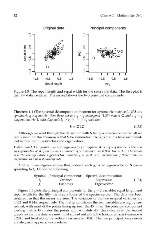
Think of the data matrix Y being the set of n points in q-dimensional space. Fororthogonal matrix G, what does the set of points W = YG look like? It looks ex-actly like Y, but rotated or flipped. Think of a pinwheel turning, or a chicken on arotisserie, or the earth spinning around its axis or rotating about the sun. Figure 1.5illustrates a simple rotation of two variables. In particular, the norms of the points inY are the same as in W, so each point remains the same distance from 0.
Rotating point clouds for three variables work by first multiplying the n × 3 datamatrix by a 3 × 3 orthogonal matrix, then making a scatter plot of the first two re-sulting variables. By running through the orthogonal matrices smoothly, one gets theillusion of three dimensions. See the discussion immediately above Exercise 1.9.23for some suggestions on software for real-time rotations.
1.6 Principal components
The grand tours and rotating point clouds described in the last two subsections donot have mathematical objectives, that is, one just looks at them to see if anythinginteresting pops up. In projection pursuit [Huber, 1985], one looks for a few (oftenjust one or two) (orthonormal) linear combinations that maximize a given objectivefunction. For example, if looking at just one linear combination, one may wish to findthe one that maximizes the variance of the data, or the skewness or kurtosis, or onewhose histogram is most bimodal. With two linear combinations, one may be afterclusters of points, high correlation, curvature, etc.
Principal components are the orthonormal combinations that maximize the vari-ance. They predate the term projection pursuit by decades [Pearson, 1901], and are themost commonly used. The idea behind them is that variation is information, so ifone has several variables, one wishes the linear combinations that capture as muchof the variation in the data as possible. You have to decide in particular situationswhether variation is the important criterion. To find a column vector b to maximizethe sample variance of W = Yb, we could take b infinitely large, which yields infinitevariance. To keep the variance meaningful, we restrict to vectors b of unit norm.
For q variables, there are q principal components: The first has the maximal vari-ance any one linear combination (with norm 1) can have, the second has the maximalvariance among linear combinations orthogonal to the first, etc. The technical defi-nition for a data matrix is below. First, we note that for a given q × p matrix B, themean and variance of the elements in the linear transformation W = YB are easily

1.6. Principal components 11
obtained from the mean and covariance matrix of Y using (1.8) and (1.15):
w =1
n1′nW =
1
n1′nYB = yB, (1.26)
by (1.9), and
SW =1
nW′HnW =
1
nB′Y′HnYB = B′SB, (1.27)
where S is the covariance matrix of Y in (1.17). In particular, for a column vector b,the sample variance of Yb is b′Sb. Thus the principal components aim to maximizeg′Sg for g’s of unit length.
Definition 1.2. Suppose S is the sample covariance matrix for the n × q data matrix Y. Letg1, . . . , gq be an orthonormal set of q × 1 vectors such that
g1 is any g that maximizes g′Sg over ‖g‖ = 1;
g2 is any g that maximizes g′Sg over ‖g‖ = 1, g′g1 = 0;
g3 is any g that maximizes g′Sg over ‖g‖ = 1, g′g1 = g′g2 = 0;
...
gq is any g that maximizes g′Sg over ‖g‖ = 1, g′g1 = · · · = g′gq−1 = 0. (1.28)
Then Ygi is the ith sample principal component, gi is its loading vector, and li ≡ g′iSgi
is its sample variance.
Because the function g′Sg is continuous in g, and the maximizations are overcompact sets, these principal components always exist. They may not be unique,although for sample covariance matrices, if n ≥ q, they almost always are unique, upto sign. See Section 13.1 and Exercise 13.4.3 for further discussion.
By the construction in (1.28), we have that the sample variances of the principalcomponents are ordered as
l1 ≥ l2 ≥ · · · ≥ lq. (1.29)
What is not as obvious, but quite important, is that the principal components areuncorrelated, as in the next lemma, proved in Section 1.8.
Lemma 1.1. The S and g1, . . . , gq in Definition 1.2 satisfy
g′iSgj = 0 for i 6= j. (1.30)
Now G ≡ (g1, . . . , gq) is an orthogonal matrix, and the matrix of principal com-ponents is
W = YG. (1.31)
Equations (1.29) and (1.30) imply that the sample covariance matrix, say L, of W isdiagonal, with the li’s on the diagonal. Hence by (1.27),
SW = G′SG = L =
l1 0 · · · 00 l2 · · · 0...
.... . .
...0 0 · · · lq
⇒ S = GLG′. (1.32)
Thus we have the following.
12 Chapter 1. Multivariate Data
−1.5 −0.5 0.5 1.5
−1.
5−
0.5
0.5
1.5
Sepal length
Sep
al w
idth
Original data
−1.5 −0.5 0.5 1.5
−1.
5−
0.5
0.5
1.5
PC1
PC
2
Principal components
Figure 1.5: The sepal length and sepal width for the setosa iris data. The first plot isthe raw data, centered. The second shows the two principal components.
Theorem 1.1 (The spectral decomposition theorem for symmetric matrices). If S is asymmetric q × q matrix, then there exists a q × q orthogonal (1.25) matrix G and a q × qdiagonal matrix L with diagonals l1 ≥ l2 ≥ · · · ≥ lq such that
S = GLG′. (1.33)
Although we went through the derivation with S being a covariance matrix, all wereally need for this theorem is that S be symmetric. The gi’s and li’s have mathemat-ical names, too: Eigenvectors and eigenvalues.
Definition 1.3 (Eigenvalues and eigenvectors). Suppose A is a q × q matrix. Then λ isan eigenvalue of A if there exists a nonzero q × 1 vector u such that Au = λu. The vectoru is the corresponding eigenvector. Similarly, u 6= 0 is an eigenvector if there exists aneigenvalue to which it corresponds.
A little linear algebra shows that, indeed, each gi is an eigenvector of S corre-sponding to li. Hence the following:
Symbol Principal components Spectral decompositionli Variance Eigenvaluegi Loadings Eigenvector
(1.34)
Figure 1.5 plots the principal components for the q = 2 variables sepal length andsepal width for the fifty iris observations of the species setosa. The data has beencentered, so that the means are zero. The variances of the two original variables are0.124 and 0.144, respectively. The first graph shows the two variables are highly cor-related, with most of the points lining up near the 45 line. The principal componentloading matrix G rotates the points approximately 45 clockwise as in the secondgraph, so that the data are now most spread out along the horizontal axis (variance is0.234), and least along the vertical (variance is 0.034). The two principal componentsare also, as it appears, uncorrelated.
1.6. Principal components 13
Best K components
In the process above, we found the principal components one by one. It may bethat we would like to find the rotation for which the first K variables, say, have themaximal sum of variances. That is, we wish to find the orthonormal set of q × 1vectors b1, . . . , bK to maximize
b′1Sb1 + · · ·+ b′
KSbK. (1.35)
Fortunately, the answer is the same, i.e., take bi = gi for each i, the principal com-ponent loadings. See Proposition 1.1 in Section 1.8. Section 13.1 explores principalcomponents further.
1.6.1 Biplots
When plotting observations using the first few principal component variables, therelationship between the original variables and principal components is often lost.An easy remedy is to rotate and plot the original axes as well. Imagine in the originaldata space, in addition to the observed points, one plots arrows of length λ along theaxes. That is, the arrows are the line segments
ai = (0, . . . , 0, c, 0, . . . , 0)′ | 0 < c < λ (the c is in the ith slot), (1.36)
where an arrowhead is added at the non-origin end of the segment. If Y is the matrixof observations, and G1 the matrix containing the first p loading vectors, then
X = YG1. (1.37)
We also apply the transformation to the arrows:
A = (a1, . . . , aq)G1. (1.38)
The plot consisting of the points X and the arrows A is then called the biplot. See
Gabriel [1981]. The points of the arrows in A are just
λIqG1 = λG1, (1.39)
so that in practice all we need to do is for each axis, draw an arrow pointing from
the origin to λ× (the ith row of G1). The value of λ is chosen by trial-and-error, sothat the arrows are amidst the observations. Notice that the components of thesearrows are proportional to the loadings, so that the length of the arrows representsthe weight of the corresponding variables on the principal components.
1.6.2 Example: Sports data
Louis Roussos asked n = 130 people to rank seven sports, assigning #1 to the sportthey most wish to participate in, and #7 to the one they least wish to participate in.The sports are baseball, football, basketball, tennis, cycling, swimming and jogging.Here are a few of the observations:

14 Chapter 1. Multivariate Data
Obs i BaseB FootB BsktB Ten Cyc Swim Jog1 1 3 7 2 4 5 62 1 3 2 5 4 7 63 1 3 2 5 4 7 6...
......
......
......
...129 5 7 6 4 1 3 2130 2 1 6 7 3 5 4
(1.40)
E.g., the first person likes baseball and tennis, but not basketball or jogging (too muchrunning?).
We find the principal components. The data is in the matrix sportsranks. It is easierto interpret the plot if we reverse the ranks, so that 7 is best and 1 is worst, then centerthe variables. The function eigen calculates the eigenvectors and eigenvalues of itsargument, returning the results in the components vectors and values, respectively:
y <− 8−sportsranksy <− scale(y,scale=F) # Centers the columnseg <− eigen(var(y))
The function prcomp can also be used. The eigenvalues (variances) are
j 1 2 3 4 5 6 7lj 10.32 4.28 3.98 3.3 2.74 2.25 0
(1.41)
The first eigenvalue is 10.32, quite a bit larger than the second. The second throughsixth are fairly equal, so it may be reasonable to look at just the first component.(The seventh eigenvalue is 0, but that follows because the rank vectors all sum to1 + · · ·+ 7 = 28, hence exist in a six-dimensional space.)
We create the biplot using the first two dimensions. We first plot the people:
ev <− eg$vectorsw <− y%∗%ev # The principal componentsr <− range(w)plot(w[,1:2],xlim=r,ylim=r,xlab=expression(’PC’[1]),ylab=expression(’PC’[2]))
The biplot adds in the original axes. Thus we want to plot the seven (q = 7) points asin (1.39), where G1 contains the first two eigenvectors. Plotting the arrows and labels:
arrows(0,0,5∗ev[,1],5∗ev[,2])text(7∗ev[,1:2],labels=colnames(y))
The constants “5” (which is the λ) and “7” were found by trial and error so that thegraph, Figure 1.6, looks good. We see two main clusters. The left-hand cluster ofpeople is associated with the team sports’ arrows (baseball, football and basketball),and the right-hand cluster is associated with the individual sports’ arrows (cycling,swimming, jogging). Tennis is a bit on its own, pointing south.

1.7. Other projections to pursue 15
−4 −2 0 2 4
−4
−2
02
4BaseB
FootB
BsktB
Ten
Cyc
Swim
Jog
PC1
PC
2
Figure 1.6: Biplot of the sports data, using the first two principal components.
1.7 Other projections to pursue
Principal components can be very useful, but you do have to be careful. For one, theydepend crucially on the scaling of your variables. For example, suppose the data sethas two variables, height and weight, measured on a number of adults. The variance
of height, in inches, is about 9, and the variance of weight, in pounds, is 900 (= 302).One would expect the first principal component to be close to the weight variable,because that is where the variation is. On the other hand, if height were measured inmillimeters, and weight in tons, the variances would be more like 6000 (for height)and 0.0002 (for weight), so the first principal component would be essentially theheight variable. In general, if the variables are not measured in the same units, it canbe problematic to decide what units to use for the variables. See Section 13.1.1. Onecommon approach is to divide each variable by its standard deviation, so that theresulting variables all have variance 1.
Another caution is that the linear combination with largest variance is not neces-sarily the most interesting, e.g., you may want one that is maximally correlated withanother variable, or that distinguishes two populations best, or that shows the mostclustering.
Popular objective functions to maximize, other than variance, are skewness, kur-tosis, and negative entropy. The idea is to find projections that are not normal (in thesense of the normal distribution). The hope is that these will show clustering or someother interesting feature.
Skewness measures a certain lack of symmetry, where one tail is longer than theother. For a sample x1, . . . , xn , it is measured by the normalized sample third central
16 Chapter 1. Multivariate Data
(meaning subtract the mean) moment:
Skewness =∑
ni=1(xi − x)3/n
(∑ni=1(xi − x)2/n)3/2
. (1.42)
Positive values indicate a longer tail to the right, and negative to the left. Kurtosis isthe normalized sample fourth central moment:
Kurtosis =∑
ni=1(xi − x)4/n
(∑ni=1(xi − x)2/n)2
− 3. (1.43)
The “−3” is there so that exactly normal data will have kurtosis 0. A variable withlow kurtosis is more “boxy” than the normal. One with high kurtosis tends to havethick tails and a pointy middle. (A variable with low kurtosis is platykurtic, and onewith high kurtosis is leptokurtic, from the Greek: kyrtos = curved, platys = flat, like aplatypus, and lepto = thin.) Bimodal distributions often have low kurtosis.
Entropy
(You may wish to look through Section 2.1 before reading this section.) The entropyof a random variable Y with pdf f (y) is
Entropy( f ) = −E f [log( f (Y))]. (1.44)
Entropy is supposed to measure lack of structure, so that the larger the entropy, themore diffuse the distribution is. For the normal, we have that
Entropy(N(µ, σ2)) = EN(µ,σ2)
[log(
√2πσ2) +
(Y − µ)2
2σ2
]=
1
2(1 + log(2πσ2)).
(1.45)Note that it does not depend on the mean µ, and that it increases without bound as σ2
increases. Thus maximizing entropy unrestricted is not an interesting task. However,one can imagine maximizing entropy for a given mean and variance, which leads tothe next lemma, to be proved in Section 1.8.
Lemma 1.2. The N(µ, σ2) uniquely maximizes the entropy among all pdf’s with mean µ and
variance σ2.
Thus a measure of non-normality of g is its entropy subtracted from that of thenormal with the same variance. Since there is a negative sign in front of the entropyof g, this difference is called negentropy defined for any g as
Negent(g) =1
2(1 + log(2πσ2))− Entropy(g), where σ2 = Varg [Y]. (1.46)
This value is known as the Kullback-Leibler distance, or discrimination information,from g to the normal density. See Kullback and Leibler [1951]. With data, the pdf gis unknown, so that the negentropy must be estimated.

1.7. Other projections to pursue 17
s
sss
s
s
ss
s
s
s
s
ss
s
s
s
s
ss
ss
sss
s
sss
ss
s
ss
ss
s s
s
ss
s
s
s
s
s
s
s
s
s
vvv
v
vv
v
v
v
v
v
v
v
vv
v
vv
vv
v
vv
vvv
vv
v
vvv
vvv
vv
v
v
vv
v
v
v
v
vvv
v
v
g
g
gg
gg
g
g
g
g
g
g
g
g
g
gg
g
g
g
g
g
g
g
gg
ggg
gg
g
ggg
g gg
g
ggg
g
ggg
g
g
g
g
3 2 1 0 −1 −2
21
0−
1−
2
PC1
PC
2
Variance
sssssssssssssss
sssss
s
ss
ss
sssssss
ss
sss
ssss
s
sss
s
ssss
vvvvv
vvv
v
v
v
v
v
vv
v
vv
v
v
v
v
vvvvvv
vvvvv v
vv
v
v
v
vvvvv v
vvv
v v gg
ggg
g
g
gg
gg
gggggg g
g
g
gg
g
ggg
gg
ggg
gggg
g
ggg
gggg ggggg
gg
3 2 1 0 −1 −2
21
0−
1−
2
Ent1E
nt2
Entropy
Figure 1.7: Projection pursuit for the iris data. The first plot is based on maximizingthe variances of the projections, i.e., principal components. The second plot maxi-mizes estimated entropies.
1.7.1 Example: Iris data
Consider the first three variables of the iris data (sepal length, sepal width, and petallength), normalized so that each variable has mean zero and variance one. We findthe first two principal components, which maximize the variances, and the first twocomponents that maximize the estimated entropies, defined as in Definition 1.28,but with estimated entropy of Yg substituted for the variance g′Sg. The table (1.47)contains the loadings for the variables. Note that the two objective functions doproduce different projections. The first principal component weights equally on thetwo length variables, while the first entropy variable is essentially petal length.
Variance Entropyg1 g2 g∗
1 g∗2
Sepal length 0.63 0.43 0.08 0.74Sepal width −0.36 0.90 0.00 −0.68Petal length 0.69 0.08 −1.00 0.06
(1.47)
Figure 1.7 graphs the results. The plots both show separation between setosa andthe other two species, but the principal components plot has the observations morespread out, while the entropy plot shows the two groups much tighter.
The matrix iris has the iris data, with the first four columns containing the mea-surements, and the fifth specifying the species. The observations are listed with thefifty setosas first, then the fifty versicolors, then the fifty virginicas. To find the prin-cipal components for the first three variables, we use the following:
y <− scale(as.matrix(iris[,1:3]))g <− eigen(var(y))$vectorspc <− y%∗%g

18 Chapter 1. Multivariate Data
The first statement centers and scales the variables. The plot of the first two columnsof pc is the first plot in Figure 1.7. The procedure we used for entropy is negent3D inListing A.3, explained in Appendix A.1. The code is
gstar <− negent3D(y,nstart=10)$vectorsent <−y%∗%gstar
To create plots like the ones in Figure 1.7, use
par(mfrow=c(1,2))sp <− rep(c(’s’,’v’,’g’),c(50,50,50))plot(pc[,1:2],pch=sp) # pch specifies the characters to plot.plot(ent[,1:2],pch=sp)
1.8 Proofs
Proof of the principal components result, Lemma 1.1
The idea here is taken from Davis and Uhl [1999]. Consider the g1, . . . , gq as definedin (1.28). Take i < j, and for angle θ, let
h(θ) = g(θ)′Sg(θ) where g(θ) = cos(θ)gi + sin(θ)gj. (1.48)
Because the gi’s are orthogonal,
‖g(θ)‖ = 1 and g(θ)′g1 = · · · = g(θ)′gi−1 = 0. (1.49)
According to the ith stage in (1.28), h(θ) is maximized when g(θ) = gi, i.e., whenθ = 0. The function is differentiable, hence its derivative must be zero at θ = 0. Toverify (1.30), differentiate:
0 =d
dθh(θ)|θ=0
=d
dθ(cos2(θ)g′
iSgi + 2 sin(θ) cos(θ)g′iSgj + sin2(θ)g′
jSgj)|θ=0
= 2g′iSgj. (1.50)
Best K components
We next consider finding the set b1, . . . , bK of orthonormal vectors to maximize the
sum of variances, ∑Ki=1 b′
iSbi, as in (1.35). It is convenient here to have the nextdefinition.
Definition 1.4 (Trace). The trace of an m × m matrix A is the sum of its diagonals,trace(A) = ∑
mi=1 aii.
Thus if we let B = (b1, . . . , bK), we have that
K
∑i=1
b′iSbi = trace(B′SB). (1.51)
1.8. Proofs 19
Proposition 1.1. Best K components. Suppose S is a q × q covariance matrix, and defineBK to be the set of q × K matrices with orthonormal columns, 1 ≤ K ≤ q. Then
maxB∈BK
trace(B′SB) = l1 + · · ·+ lK, (1.52)
which is achieved by taking B = (g1, . . . , gK), where gi is the ith principal component loadingvector for S, and li is the corresponding variance.
Proof. Let GLG′ be the spectral decomposition of S as in (1.33). Set A = G′B, so thatA is also in BK . Then B = GA, and
trace(B′SB) = trace(A′G′SGA)
= trace(A′LA)
=q
∑i=1
[(K
∑j=1
a2ij)li]
=q
∑i=1
cili, (1.53)
where the aij’s are the elements of A, and ci = ∑Kj=1 a2
ij. Because the columns of A
have norm one, and the rows of A have norms less than or equal to one,
q
∑i=1
ci =K
∑j=1
[q
∑i=1
a2ij] = K and ci ≤ 1. (1.54)
Since l1 ≥ l2 ≥ · · · ≥ lq, to maximize (1.53) under those constraints on the ci’s, we tryto make the earlier ci’s as large as possible. Thus we set c1 = · · · = cK = 1 and cK+1 =· · · = cq = 0. The resulting value of (1.53) is then l1 + · · ·+ lK. Note that taking Awith aii = 1, i = 1, . . . , K, and 0 elsewhere (so that A consists of the first K columnsof Iq), achieves that maximum. With that A, we have that B = (g1, . . . , gK).
Proof of the entropy result, Lemma 1.2
Let f be the N(µ, σ2) density, and g be any other pdf with mean µ and variance σ2.Then
Entropy( f )− Entropy(g) =−∫
f (y) log( f (y))dy +∫
g(y) log(g(y))dy
=∫
g(y) log(g(y))dy −∫
g(y) log( f (y))dy
+∫
g(y) log( f (y))dy −∫
f (y) log( f (y))dy
=−∫
g(y) log( f (y)/g(y))dy
+ Eg
[log(
√2πσ2) +
(Y − µ)2
2σ2
]
− E f
[log(
√2πσ2) +
(Y − µ)2
2σ2
](1.55)
=Eg[− log( f (Y)/g(Y))]. (1.56)
20 Chapter 1. Multivariate Data
The last two terms in (1.55) are equal, since Y has the same mean and variance underf and g.
At this point we need an important inequality about convexity, to whit, whatfollows is a definition and lemma.
Definition 1.5 (Convexity). The real-valued function h, defined on an interval I ⊂ R, isconvex if for each x0 ∈ I, there exists an a0 and b0 such that
h(x0) = a0 + b0x0 and h(x) ≥ a0 + b0x for x 6= x0. (1.57)
The function is strictly convex if the inequality is strict in (1.57).
The line a0 + b0x is the tangent line to h at x0. Convex functions have tangentlines that are below the curve, so that convex functions are “bowl-shaped.” The nextlemma is proven in Exercise 1.9.15.
Lemma 1.3 (Jensen’s inequality). Suppose W is a random variable with finite expectedvalue. If h(w) is a convex function, then
E[h(W)] ≥ h(E[W]), (1.58)
where the left-hand expectation may be infinite. Furthermore, the inequality is strict if h(w)is strictly convex and W is not constant, that is, P[W = c] < 1 for any c.
One way to remember the direction of the inequality is to imagine h(w) = w2,
in which case (1.58) states that E[W2] ≥ E[W]2, which we already know because
Var[X] = E[W2]− E[W]2 ≥ 0.Now back to (1.56). The function h(w) = − log(w) is strictly convex, and if g is
not equivalent to f , W = f (Y)/g(Y) is not constant. Jensen’s inequality thus showsthat
Eg[− log( f (Y)/g(Y))] > − log (E[ f (Y)/g(Y)])
= − log
(∫( f (y)/g(y))g(y)dy
)
= − log
(∫f (y)dy
)= − log(1) = 0. (1.59)
Putting (1.56) and (1.59) together yields
Entropy(N(0, σ2))− Entropy(g) > 0, (1.60)
which completes the proof of Lemma 1.2.
Answers: The question marks in Figure 1.4 are, respectively, virginica, setosa,virginica, versicolor, and setosa.
1.9 Exercises
Exercise 1.9.1. Let Hn be the centering matrix in (1.12). (a) What is Hn1n? (b) Supposex is an n × 1 vector whose elements sum to zero. What is Hnx? (c) Show that Hn isidempotent (1.16).

1.9. Exercises 21
Exercise 1.9.2. Define the matrix Jn = (1/n)1n1′n, so that Hn = In − Jn. (a) Whatdoes Jn do to a vector? (That is, what is Jna?) (b) Show that Jn is idempotent. (c) Findthe spectral decomposition (1.33) for Jn explicitly when n = 3. [Hint: In G, the firstcolumn (eigenvector) is proportional to 13. The remaining two eigenvectors can beany other vectors such that the three eigenvectors are orthonormal. Once you have aG, you can find the L.] (d) Find the spectral decomposition for H3. [Hint: Use thesame eigenvectors as for J3, but in a different order.] (e) What do you notice aboutthe eigenvalues for these two matrices?
Exercise 1.9.3. A covariance matrix has intraclass correlation structure if all the vari-ances are equal, and all the covariances are equal. So for n = 3, it would look like
A =
a b bb a bb b a
. (1.61)
Find the spectral decomposition for this type of matrix. [Hint: Use the G in Exercise1.9.2, and look at G′AG. You may have to reorder the eigenvectors depending on thesign of b.]
Exercise 1.9.4. Show (1.24): if the q × p matrix B has orthonormal columns, thenB′B = Ip.
Exercise 1.9.5. Suppose Y is an n × q data matrix, and W = YG, where G is a q × qorthogonal matrix. Let y1, . . . , yn be the rows of Y, and similarly wi’s be the rows ofW. (a) Show that the corresponding points have the same length: ‖yi‖ = ‖wi‖. (b)Show that the distances between the points have not changed: ‖yi − yj‖ = ‖wi − wj‖,for any i, j.
Exercise 1.9.6. Show that the construction in Definition 1.1 implies that the variancessatisfy (1.30): l1 ≥ l2 ≥ · · · ≥ lq.
Exercise 1.9.7. Suppose that the columns of G constitute the principal componentloading vectors for the sample covariance matrix S. Show that g′
iSgi = li and g′iSgj =
0 for i 6= j, as in (1.30), implies (1.32): G′SG = L.
Exercise 1.9.8. Verify (1.49) and (1.50).
Exercise 1.9.9. In (1.53), show that trace(A′LA) = ∑qi=1[(∑
Kj=1 a2
ij)li].
Exercise 1.9.10. This exercise is to show that the eigenvalue matrix of a covariancematrix S is unique. Suppose S has two spectral decompositions, S = GLG′ = HMH′,where G and H are orthogonal matrices, and L and M are diagonal matrices withnonincreasing diagonal elements. Use Proposition 1.1 on both decompositions of Sto show that for each K = 1, . . . , q, l1 + · · ·+ lK = m1 + · · ·+ mK. Thus L = K.
Exercise 1.9.11. Suppose Y is a data matrix, and Z = YF for some orthogonal matrixF, so that Z is a rotated version of Y. Show that the variances of the principal com-ponents are the same for Y and Z. (This result should make intuitive sense.) [Hint:Find the spectral decomposition of the covariance of Z from that of Y, then note thatthese covariance matrices have the same eigenvalues.]
Exercise 1.9.12. Show that in the spectral decomposition (1.33), each li is an eigen-value, with corresponding eigenvector gi, i.e., Sgi = ligi.

22 Chapter 1. Multivariate Data
Exercise 1.9.13. Suppose λ is an eigenvalue of the covariance matrix S. Show thatλ must equal one of the li’s in the spectral decomposition of S. [Hint: Let u bean eigenvector corresponding to λ. Show that λ is also an eigenvalue of L, withcorresponding eigenvector v = G′u, so that livi = λvi for each i. Why does that factlead to the desired result?]
Exercise 1.9.14. Verify the expression for∫
g(y) log( f (y))dy in (1.55).
Exercise 1.9.15. Consider the setup in Jensen’s inequality, Lemma 1.3. (a) Show thatif h is convex, E[h(W)] ≥ h(E[W]). [Hint: Set x0 = E[W] in Definition 1.5.] (b)Suppose h is strictly convex. Give an example of a random variable W for whichE[h(W)] = h(E[W]). (c) Show that if h is strictly convex and W is not constant, thatE[h(W)] > E[W].
Exercise 1.9.16 (Spam). In the Hewlett-Packard spam data, n = 4601 emails wereclassified according to whether they were spam, where “0” means not spam, “1”means spam. Fifty-seven explanatory variables based on the content of the emailswere recorded, including various word and symbol frequencies. The emails weresent to George Forman (not the boxer) at Hewlett-Packard labs, hence emails withthe words “George” or “hp” would likely indicate non-spam, while “credit” or “!”would suggest spam. The data were collected by Hopkins et al. [1999], and are in thedata matrix Spam. (They are also in the R data frame spam from the ElemStatLearnpackage [Halvorsen, 2012], as well as at the UCI Machine Learning Repository [Lich-man, 2013].)
Based on an email’s content, is it possible to accurately guess whether it is spamor not? Here we use Chernoff’s faces. Look at the faces of some emails known tobe spam and some known to be non-spam (the “training data”). Then look at somerandomly chosen faces (the “test data”). E.g., to have twenty observations knownto be spam, twenty known to be non-spam, and twenty test observations, use thefollowing R code:
x0 <− Spam[Spam[,’spam’]==0,] # The non−spamx1 <− Spam[Spam[,’spam’]==1,] # The spamtrain0 <− x0[1:20,]train1 <− x1[1:20,]test <− rbind(x0[−(1:20),],x1[−(1:20),])[sample(1:4561,20),]
Based on inspecting the training data, try to classify the test data. How accurate areyour guesses? The faces program uses only the first fifteen variables of the inputmatrix, so you should try different sets of variables. For example, for each variablefind the value of the t-statistic for testing equality of the spam and email groups, thenchoose the variables with the largest absolute t’s.
Exercise 1.9.17 (Spam). Continue with the spam data from Exercise 1.9.16. (a) Plot thevariances of the explanatory variables (the first 57 variables) versus the index (i.e., thex-axis has (1, 2, . . . , 57), and the y-axis has the corresponding variances.) You mightnot see much, so repeat the plot, but taking logs of the variances. What do you see?Which three variables have the largest variances? (b) Find the principal componentsusing just the explanatory variables. Plot the eigenvalues versus the index. Plot thelog of the eigenvalues versus the index. What do you see? (c) Look at the loadings forthe first three principal components. (E.g., if spamload contains the loadings (eigen-vectors), then you can try plotting them using matplot(1:57,spamload[,1:3]).) Whatis the main feature of the loadings? How do they relate to your answer in part (a)?

1.9. Exercises 23
(d) Now scale the explanatory variables so each has mean zero and variance one:spamscale <− scale(Spam[,1:57]). Find the principal components using this matrix.Plot the eigenvalues versus the index. What do you notice, especially compared tothe results of part (b)? (e) Plot the loadings of the first three principal componentsobtained in part (d). How do they compare to those from part (c)? Why is there sucha difference?
Exercise 1.9.18 (Sports data). Consider the Louis Roussos sports data described inSection 1.6.2. Use faces to cluster the observations. Use the raw variables, or the prin-cipal components, and try different orders of the variables (which maps the variablesto different sets of facial features). After clustering some observations, look at howthey ranked the sports. Do you see any pattern? Were you able to distinguish be-tween people who like team sports versus individual sports? Those who like (dislike)tennis? Jogging?
Exercise 1.9.19 (Election). The data set election has the results of the first three USpresidential races of the 2000’s (2000, 2004, 2008). The observations are the 50 statesplus the District of Columbia, and the values are the (D − R)/(D + R) for each stateand each year, where D is the number of votes the Democrat received, and R is thenumber the Republican received. (a) Without scaling the variables, find the principalcomponents. What are the first two principal component loadings measuring? Whatis the ratio of the standard deviation of the first component to the second’s? (c) Plotthe first versus second principal components, using the states’ two-letter abbrevia-tions as the plotting characters. (They are in the vector stateabb.) Make the plot sothat the two axes cover the same range. (d) There is one prominent outlier. Whatis it, and for which variable is it mostly outlying? (e) Comparing how states aregrouped according to the plot and how close they are geographically, can you makeany general statements about the states and their voting profiles (at least for thesethree elections)?
Exercise 1.9.20 (Painters). The data set painters has ratings of 54 famous painters. Itis in the MASS package [Venables and Ripley, 2002]. See Davenport and Studdert-Kennedy [1972] for a more in-depth discussion. The R help file says
The subjective assessment, on a 0 to 20 integer scale, of 54 classical paint-ers. The painters were assessed on four characteristics: composition,drawing, colour and expression. The data is due to the Eighteenth centuryart critic, de Piles.
The fifth variable gives the school of the painter, using the following coding:
A: Renaissance; B: Mannerist; C: Seicento; D: Venetian; E: Lombard; F:Sixteenth Century; G: Seventeenth Century; H: French
Create the two-dimensional biplot for the data. Start by turning the data into a matrix,then centering both dimensions, then scaling:
x <− scale(as.matrix(painters[,1:4]),scale=F)x <− t(scale(t(x),scale=F))x <− scale(x)
Use the fifth variable, the painters’ schools, as the plotting character, and the fourrating variables as the arrows. Interpret the two principal component variables. Canyou make any generalizations about which schools tend to rate high on which scores?
24 Chapter 1. Multivariate Data
Exercise 1.9.21 (Cereal). Chakrapani and Ehrenberg [1981] analyzed people’s atti-tudes towards a variety of breakfast cereals. The data matrix cereal is 8 × 11, withrows corresponding to eight cereals, and columns corresponding to potential at-tributes about cereals. The attributes: Return (a cereal one would come back to),tasty, popular (with the entire family), digestible, nourishing, natural flavor, afford-able, good value, crispy (stays crispy in milk), fit (keeps one fit), and fun (for children).The original data consisted of the percentage of subjects who thought the given ce-real possessed the given attribute. The present matrix has been doubly centered, sothat the row means and columns means are all zero. (The original data can be found
in the S-Plus® [TIBCO Software Inc., 2009] data set cereal.attitude.) Create the two-dimensional biplot for the data with the cereals as the points (observations), and theattitudes as the arrows (variables). What do you see? Are there certain cereals/at-tributes that tend to cluster together? (You might want to look at the Wikipedia entry[Wikipedia, 2015] on breakfast cereals.)
Exercise 1.9.22 (Decathlon). The decathlon data set has scores on the top 24 men inthe decathlon (a set of ten events) at the 2008 Olympics. The scores are the numbersof points each participant received in each event, plus each person’s total points. See[Wikipedia, 2014a]. Create the biplot for these data based on the first ten variables(i.e., do not use their total scores). Doubly center, then scale, the data as in Exercise1.9.20. The events should be the arrows. Do you see any clustering of the events? Theathletes?
The remaining questions require software that will display rotating point clouds ofthree dimensions, and calculate some projection pursuit objective functions. The Spinprogram at http://istics.net/Spin is sufficient for our purposes. GGobi [Cookand Swayne, 2007] has an excellent array of graphical tools for interactively exploringmultivariate data. See also Wickham et al. [2011] and the spin3R routine in the Rpackage aplpack [Wolf, 2014].
Exercise 1.9.23 (Iris). Consider the three variables X = sepal length, Y = petal length,and Z = petal width in the Fisher-Anderson iris data. (a) Look at the data whilerotating. What is the main feature of these three variables? (b) Scale the data so thatthe variables all have the same sample variance. (The Spin program automaticallyperforms the scaling.) For various objective functions (variance, skewness, kurtosis,negative kurtosis, negentropy), find the rotation that maximizes the function. (Thatis, the first component of the rotation maximizes the criterion over all rotations. Thesecond then maximizes the criterion for components orthogonal to the first. The thirdcomponent is then whatever is orthogonal to the first two.) Which criteria are mosteffective in yielding rotations that exhibit the main feature of the data? Which areleast effective? (c) Which of the original variables are most prominently representedin the first two components of the most effective rotations?
Exercise 1.9.24 (Automobiles). The data set cars [Consumers’ Union, 1990] containsq = 11 size measurements on n = 111 models of automobile. The original data can be
found in the S-Plus® [TIBCO Software Inc., 2009] data frame cu.dimensions. In cars,the variables have been normalized to have medians of 0 and median absolute devi-ations (MAD) of 1.4826 (the MAD for a N(0, 1)). Inspect the three-dimensional dataset consisting of the variables length, width, and height. (In the Spin program, thedata set is called “Cars.”) (a) Find the linear combination with the largest variance.
1.9. Exercises 25
What is the best linear combination? (Can you interpret it?) What is its variance?Does the histogram look interesting? (b) Now find the linear combination to maxi-mize negentropy. What is the best linear combination, and its entropy? What is themain feature of the histogram? (c) Find the best two linear combinations for entropy.What are they? What feature do you see in the scatter plot?
Exercise 1.9.25 (RANDU). RANDU [IBM, 1970] is a venerable, fast, efficient, and veryflawed random number generator. See Dudewicz and Ralley [1981] for a thorough re-view of old-time random number generators. For given “seed” x0, RANDU producesxi+1 from xi via
xi+1 = (65539 xi) mod 231. (1.62)
The “random” Uniform(0,1) values are then ui = xi/231. The R data set randu isbased on a sequence generated using RANDU, where each of n = 400 rows is a setof p = 3 consecutive ui’s. Rotate the data, using objective criteria if you wish, to lookfor significant nonrandomness in the data matrix. If the data are really random, thepoints should uniformly fill up the three-dimensional cube. What feature do you seethat reveals the nonrandomness?
The data sets Example 1, Example 2, . . ., Example 5 are artificial three-dimensionalpoint clouds. The goal is to rotate the point clouds to reveal their structures.
Exercise 1.9.26. Consider the Example 1 data set. (a) Find the first two principalcomponents for these data. What are their variances? (b) Rotate the data. Are theprincipal components unique? (c) Find the two-dimensional plots based on maximiz-ing the skewness, kurtosis, negative kurtosis, and negentropy criteria. What do yousee? What does the histogram for the linear combination with the largest kurtosislook like? Is it “pointy”? What does the histogram for the linear combination withthe most negative kurtosis look like? Is it “boxy”? (d) Describe the three-dimensionalstructure of the data points. Do the two-dimensional plots in part (c) give a goodidea of the three-dimensional structure?
Exercise 1.9.27. This question uses the Example 2 data set. (a) What does the his-togram for the linear combination with the largest variance look like? (b) What doesthe histogram for the linear combination with the largest negentropy look like? (c)Describe the three-dimensional object.
Exercise 1.9.28. For each of Example 3, 4, and 5, try to guess the shape of the cloudof data points based on just the 2-way scatter plots. Then rotate the points enough toconvince yourself of the actual shape.


Chapter 2
Multivariate Distributions
This chapter reviews the elements of distribution theory that we need, especially forvectors and matrices. (Classical multivariate analysis is basically linear algebra, soeverything we do eventually gets translated into matrix equations.) See any goodmathematical statistics book such as Hogg, McKean, and Craig [2012], Bickel andDoksum [2000], or Lehmann and Casella [2003] for a more comprehensive treatment.
2.1 Probability distributions
We will deal with random variables and finite collections of random variables. Arandom variable X has range or space X ⊂ R, the real line. A collection of ran-dom variables is a finite set of random variables. They could be arranged in anyconvenient way, such as a row or column vector, matrix, triangular array, or three-dimensional array, and will often be indexed to match the arrangement. The defaultarrangement will be to index the random variables by 1, . . . , N, so that the collec-
tion is X = (X1, . . . , XN), considered as a row vector. The space of X is X ⊂ RN ,N-dimensional Euclidean space. A probability distribution P for a random variableor collection of random variables specifies the chance that the random object will fallin a particular subset of its space. That is, for A ⊂ X , P[A] is the probability thatthe random X is in A, also written P[X ∈ A]. In principle, to describe a probabilitydistribution, one must specify P[A] for all subsets A. (Technically, all “measurable”subsets, but we will not worry about measurability.) Fortunately, there are easierways. We will use densities, but the main method will be to use representations, bywhich we mean describing a collection of random variables Y in terms of anothercollection X for which we already know the distribution, usually through a function,i.e., Y = g(X).
2.1.1 Distribution functions
The distribution function for the probability distribution P for the collection X =(X1, . . . , XN) of random variables is the function
F : RN → [0, 1]
F(x1, x2, . . . , xN) = P[X1 ≤ x1, X2 ≤ x2, . . . , XN ≤ xN ]. (2.1)
27

28 Chapter 2. Multivariate Distributions
Note that it is defined on all of RN , not just the space of X. It is nondecreasing, andcontinuous from the right, in each xi. The limit as all xi → −∞ is zero, and as allxi → ∞, the limit is one. The distribution function uniquely defines the distribution,though we will not find much use for it.
2.1.2 Densities
A collection of random variables X is said to have a density with respect to Lebesguemeasure on RN , if there is a nonnegative function f (x),
f : X −→ [0, ∞), (2.2)
such that for any A ⊂ X ,
P[A] =∫
Af (x)dx
=∫ ∫
· · ·∫
Af (x1, . . . , xN)dx1 · · · dxN . (2.3)
The second line is there to emphasize that we have a multiple integral. (The Lebesgue
measure of a subset A of RN is the integral∫
A dx, i.e., as if f (x) = 1 in (2.3). Thus ifN = 1, the Lebesgue measure of a line segment is its length. In two dimensions, theLebesgue measure of a set is its area. For N = 3, it is the volume.)
We will call a density f as in (2.3) the “pdf,” for “probability density function.”(Densities can also be defined with respect to other measures than Lebesgue, butfor our purposes, pdf means the dominating measure is Lebesgue.) Because P[X ∈X ] = 1, the integral of the pdf over the entire space X must be 1. Random variables orcollections that have pdf’s are continuous in the sense that their distribution functionsare continuous in x. (There are continuous distributions that do not have pdf’s, suchas the uniform distribution on the unit circle.)
If X does have a pdf, then it can be obtained from the distribution function in (2.1)by differentiation:
f (x1, . . . , xN) =∂N
∂x1 · · · ∂xNF(x1, . . . , xN). (2.4)
If the space X is a countable (which includes finite) set, then its probability can begiven by specifying the probability of each individual point. The probability massfunction f , or “pmf,” with
f : X −→ [0, 1], (2.5)
is given byf (x) = P[X = x] = P[x]. (2.6)
The probability of any subset A is the sum of the probabilities of the individual pointsin A,
P[A] = ∑x∈A
f (x). (2.7)
Such an X is called discrete. (A pmf is also a density, but with respect to countingmeasure on X , not Lebesgue measure.)
Not all random variables are either discrete or continuous, and especially a collec-tion of random variables could have some discrete and some continuous members. In

2.1. Probability distributions 29
such cases, the probability of a set is found by integrating over the continuous partsand summing over the discrete parts. For example, suppose our collection is a 1 × Nvector combining two other collections, i.e.,
W = (X, Y) has space W , X is 1 × Nx and Y is 1 × Ny, N = Nx + Ny. (2.8)
For a subset A ⊂ W , define the marginal space by
X A = x ∈ RNx | (x, y) ∈ A for some y, (2.9)
and the conditional space given X = x by
YAx = y ∈ RNy | (x, y) ∈ A. (2.10)
Suppose X is discrete and Y is continuous. Then f (x, y) is a mixed-type density forthe distribution of W if for any A ⊂ W ,
P[A] = ∑x∈X A
∫
YAx
f (x, y)dy. (2.11)
We will use the generic term “density” to mean pdf, pmf, or the mixed type of densityin (2.11). There are other types of densities, but we will not need to deal with them.
2.1.3 Representations
Representations are very useful, especially when no pdf exists. For example, supposeY = (Y1, Y2) is uniform on the unit circle, by which we mean Y has space Y = y ∈R2 | ‖y‖ = 1, and it is equally likely to be any point on that circle. There is no
pdf, because the area of the circle in R2 is zero, so the integral over any subset ofY of any function is zero. The distribution can be thought of in terms of the angley makes with the x-axis, that is, y is equally likely to be at any angle. Thus we canlet X ∼ Uniform(0, 2π]: X has space (0, 2π] and pdf fX(x) = 1/(2π). Then we candefine
Y = (cos(X), sin(X)). (2.12)
In general, suppose we are given the distribution for X with space X and functiong,
g : X −→ Y . (2.13)
Then for any B ⊂ Y , we can define the probability of Y by
P[Y ∈ B] = P[g(X) ∈ B] = P[X ∈ g−1(B)]. (2.14)
We know the final probability because g−1(B) ⊂ X .One special type of function yields marginal distributions, analogous to the mar-
ginals in Section 1.5, that picks off some of the components. Consider the setup in(2.8). The marginal function for X simply chooses the X components:
g(x, y) = x. (2.15)
The space of X is then given by (2.9) with A = W , i.e.,
X ≡ XW = x ∈ RNx | (x, y) ∈ W for some y. (2.16)
30 Chapter 2. Multivariate Distributions
If f (x, y) is the density for (X, Y), then the density of X can be found by “integrating(or summing) out” the y. That is, if f is a pdf, then fX(x) is the pdf for X, where
fX(x) =∫
Yx
f (x, y)dy, (2.17)
andYx = YW
x = y ∈ RNy | (x, y) ∈ W (2.18)
is the conditional space (2.10) with A = W . If y has some discrete components, thenthey are summed in (2.17).
Note that we can find the marginals of any subset, not just sets of consecutiveelements. E.g., if X = (X1, X2, X3, X4, X5), we can find the marginal of (X2, X4, X5)by integrating out the X1 and X3.
Probability distributions can also be represented through conditioning, discussedin the next section.
2.1.4 Conditional distributions
The conditional distribution of one or more variables given another set of variablesis central to multivariate analysis. E.g., what is the distribution of health measuresgiven diet, smoking, and ethnicity? We start with the two collections of variables Yand X, each of which may be a random variable, vector, matrix, etc. We want to makesense of the notion
Conditional distribution of Y given X = x, written Y |X = x. (2.19)
What this means is that for each fixed value x, there is a possibly different distributionfor Y.
Very generally, such conditional distributions will exist, though they may be hardto figure out, even what they mean. In the discrete case, the concept is straightfor-ward, and by analogy the case with densities follows. For more general situations,we will use properties of conditional distributions rather than necessarily specifyingthem.
We start with the (X, Y) as in (2.8), and assume we have their joint distributionP. The word “joint” is technically unnecessary, but helps to emphasize that we areconsidering the two collections together. The joint space is W , and let X denote themarginal space of X as in (2.16), and for each x ∈ X , the conditional space of Y givenX = x, Yx, is given in (2.18). For example, if the space W = (x, y) | 0 < x < y < 1,then X = (0, 1), and for x ∈ X , Yx = (x, 1).
Next, given the joint distribution of (X, Y), we define the conditional distribution(2.19) in the discrete, then pdf, cases.
Discrete case
For sets A and B, the conditional probability of A given B is defined as
P[A | B] =P[A ∩ B]
P[B]if B 6= ∅. (2.20)
If B is empty, then the conditional probability is not defined since we would have 00 .
For a discrete pair (X, Y), let f (x, y) be the pmf. Then the conditional distribution of

2.1. Probability distributions 31
Y given X = x can be specified by
P[Y = y | X = x], for x ∈ X , y ∈ Yx, (2.21)
at least if P[X = x] > 0. The expression in (2.21) is, for fixed x, the conditional pmffor Y:
fY|X(y | x) = P[Y = y | X = x]
=P[Y = y and X = x]
P[X = x]
=f (x, y)
fX(x), y ∈ Yx, (2.22)
if fX(x) > 0, where fX(x) is the marginal pmf of X from (2.17) with sums.
Pdf case
In the discrete case, the restriction that P[X = x] > 0 is not worrisome, since thechance is 0 we will have an x with P[X = x] = 0. In the continuous case, we cannotfollow the same procedure, since P[X = x] = 0 for all x ∈ X . However, if we havepdf’s, or general densities, we can analogize (2.22) and declare that the conditionaldensity of Y given X = x is
fY|X(y | x) =f (x, y)
fX(x), y ∈ Yx, (2.23)
if fX(x) > 0. In this case, as in the discrete one, the restriction that fX(x) > 0 is notworrisome, since the set on which X has density zero has probability zero. It turnsout that the definition (2.23) is mathematically legitimate.
The Y and X can be very general. Often, both will be functions of a collectionof random variables, so that we may be interested in conditional distributions of thetype
g(Y) | h(X) = z (2.24)
for some functions g and h.
Reconstructing the joint distribution
Note that if we are given the marginal space and density for X, and the conditionalspaces and densities for Y given X = x, then we can reconstruct the joint space andjoint density:
W = (x, y) | y ∈ Yx, x ∈ X and f (x, y) = fY|X(y | x) fX(x). (2.25)
Thus another way to represent a distribution for Y is to specify the conditionaldistribution given each X = x, and the marginal of X. The marginal distribution of Yis then found by first finding the joint as in (2.25), then integrating out the x:
fY(y) =∫
Xy
fY|X(y | x) fX(x)dx. (2.26)

32 Chapter 2. Multivariate Distributions
2.2 Expected values
Means, variances, and covariances (Section 1.4) are key sample quantities in describ-ing data. Similarly, they are important for describing random variables. These are allexpected values of some function, defined next.
Definition 2.1 (Expected value). Suppose X has space X , and consider the real-valuedfunction g,
g : X −→ R. (2.27)
If X has pdf f , then the expected value of g(X), E[g(X)], is
E[g(X)] =∫
Xg(x) f (x)dx (2.28)
if the integral converges. If X has pmf f , then
E[g(X)] = ∑x∈X
g(x) f (x) (2.29)
if the sum converges.
As in (2.11), if the collection is (X, Y), where X is discrete and Y is continuous, andf (x, y) is its mixed-type density, then for function g(x, y),
E[g(X, Y)] = ∑x∈X
∫
Yx
g(x, y) f (x, y)dy. (2.30)
if everything converges. (The spaces are defined in (2.16) and (2.18).)Expected values for representations cohere is the proper way, that is, if Y is a
collection of random variables such that Y = h(X), then for a function g,
E[g(Y)] = E[g(h(X))], (2.31)
if the latter exists. Thus we often can find the expected values of functions of Y basedon the distribution of X. See Exercise 2.7.5 for the discrete case.
Conditioning
If (X, Y) has a joint distribution, then we can define the conditional expectation ofg(Y) given X = x to be the regular expected value of g(Y), but we use the conditionaldistribution Y | X = x. In the pdf case, we write
E[g(Y) | X = x] =∫
Yx
g(y) fY|X(y|x)dy ≡ eg(x). (2.32)
Note that the conditional expectation is a function of x. We can then take the expectedvalue of that, using the marginal distribution of X. We end up with the same result(if we end up with anything) as taking the usual expected value of g(Y). That is,
E[g(Y)] = E[E[g(Y) |X = x]]. (2.33)
There is a bit of a notational glitch in the formula, since the inner expected value is afunction of x, a constant, and we really want to take the expected value over X. Wecannot just replace x with X, however, because then we would have the undesired
2.3. Means, variances, and covariances 33
E[g(Y) | X = X]. So a more precise way to express the result is to use the eg(x) in(2.32), so that
E[g(Y)] = E[eg(X)]. (2.34)
This result holds in general. It is not hard to see in the pdf case:
E[eg(X)] =∫
Xeg(x) fX(x)dx
=∫
X
∫
Yx
g(y) fY|X(y|x)dy fX(x)dx by (2.32)
=∫
X
∫
Yx
g(y) f (x, y)dydx by (2.25)
=∫
Wg(y) f (x, y)dxdy by (2.25)
= E[g(Y)]. (2.35)
A useful corollary is the total probability formula: For B ⊂ Y , if X has a pdf,
P[Y ∈ B] =∫
XP[Y ∈ B | X = x] fX(x)dx. (2.36)
If X has a pmf, then we sum. The formula follows by taking g to be the indicatorfunction IB, given as
IB(y) =
1 if y ∈ B,0 if y 6∈ B.
(2.37)
2.3 Means, variances, and covariances
Means, variances, and covariances are particular expected values. For a collectionof random variables X = (X1, . . . , XN), the mean of Xj is its expected value, E[Xj].
(Throughout this section, we will be acting as if the expected values exist. So if E[Xj]doesn’t exist, then the mean of Xj doesn’t exist, but we might not explicitly mention
that.) Often the mean is denoted by µ, so that E[Xj] = µj.
The variance of Xj, often denoted σ2j or σjj, is
σjj = Var[Xj ] = E[(Xj − µj)2]. (2.38)
The covariance between Xj and Xk is defined to be
σjk = Cov[Xj, Xk] = E[(Xj − µj)(Xk − µk)]. (2.39)
Their correlation coefficient is
Corr[Xj, Xk] = ρjk =σjk√σjjσkk
, (2.40)
if both variances are positive. Compare these definitions to those of the sampleanalogs, (1.3), (1.4), (1.5), and (1.6). So, e.g., Var[Xj] = Cov[Xj, Xj].
The mean of the collection X is the corresponding collection of means. That is,
µ = E[X] = (E[X1], . . . , E[XN ]). (2.41)
34 Chapter 2. Multivariate Distributions
2.3.1 Vectors and matrices
If a collection has a particular structure, then its mean has the same structure. Thatis, if X is a row vector as in (2.41), then E[X] = (E[X1], . . . , E[XN ]). If X is a columnvector, so is its mean. Similarly, if W is an n × p matrix, then so is its mean. That is,
E[W] = E
W11 W12 · · · W1p
W21 W22 · · · W2p
......
. . ....
Wn1 Wn2 · · · Wnp
=
E[W11] E[W12] · · · E[W1p]E[W21] E[W22] · · · E[W2p]
......
. . ....
E[Wn1] E[Wn2] · · · E[Wnp]
. (2.42)
Turning to variances and covariances, first suppose that X is a vector (row or
column). There are N variances and (N2 ) covariances among the Xj’s to consider,
recognizing that Cov[Xj, Xk] = Cov[Xk, Xj]. By convention, we will arrange them intoa matrix, the variance-covariance matrix, or simply covariance matrix of X:
Σ = Cov[X]
=
Var[X1] Cov[X1, X2] · · · Cov[X1, XN ]Cov[X2, X1] Var[X2] · · · Cov[X2, XN ]
......
. . ....
Cov[XN, X1] Cov[XN , X2] · · · Var[XN ]
, (2.43)
so that the elements of Σ are the σjk’s. Compare this arrangement to that of the
sample covariance matrix (1.17). If X is a row vector, and µ = E[X], a convenientexpression for its covariance is
Cov[X] = E[(X −µ)′(X −µ)
]. (2.44)
Similarly, if X is a column vector, Cov[X] = E[(X −µ)(X −µ)′].Now suppose X is a matrix as in (2.42). Notice that individual components have
double subscripts: Xij. We need to decide how to order the elements in order todescribe its covariance matrix. We will use the convention that the elements arestrung out by row, so that row(X) is the 1 × N vector, N = np, given by
row(X) =(X11, X12, · · · , X1p,
X21, X22, · · · , X2p,
· · ·Xn1, Xn2, · · · , Xnp). (2.45)
Then Cov[X] is defined to be Cov[row(X)], which is an (np)× (np) matrix.One more covariance: The covariance between two vectors is defined to be the
matrix containing all the individual covariances of one variable from each vector.

2.4. Independence 35
That is, if X is 1 × p and Y is 1 × q , then the p × q matrix of covariances is
Cov[X, Y] = E[(X − E[X])′(Y − E[Y])]
=
Cov[X1, Y1] Cov[X1, Y2] · · · Cov[X1, Yq]Cov[X2, Y1] Cov[X2, Y2] · · · Cov[X2, Yq]
......
. . ....
Cov[Xp, Y1] Cov[Xp, Y2] · · · Cov[Xp, Yq]
. (2.46)
2.3.2 Moment generating functions
The moment generating function (mgf for short) of X is a function from RN → [0, ∞]given by
MX(t) = MX(t1, . . . , tN) = E[et1 X1+···+tN XN
]= E
[eXt′]
(2.47)
for t = (t1, . . . , tN). It is very useful in distribution theory, especially convolutions(sums of independent random variables), asymptotics, and for generating moments.The main use we have is that the mgf determines the distribution:
Theorem 2.1 (Uniqueness of mgf). If for some ǫ > 0,
MX(t) < ∞ and MX(t) = MY(t) for all t such that ‖t‖ < ǫ, (2.48)
then X and Y have the same distribution.
See Ash [1970] for an approach to proving this result. The mgf does not alwaysexist, that is, often the integral or sum defining the expected value diverges. Thatis ok, as long as it is finite for t in a neighborhood of 0. If one knows complexvariables, the characteristic function is handy because it always exists. It is definedas φX(t) = E[exp(iXt′)].
If a distribution’s mgf is finite when ‖t‖ < ǫ for some ǫ > 0, then all of its momentsare finite, and can be calculated via differentiation:
E[Xk1
1 · · · XkN
N ] =∂K
∂tk1
1 · · · ∂tkN
N
MX(t)∣∣∣t=0
, (2.49)
where the ki are nonnegative integers, and K = k1 + · · ·+ kN . See Exercise 2.7.22.
2.4 Independence
Two sets of random variables are independent if the values of one set do not affectthe values of the other. More precisely, suppose the collection is (X, Y) as in (2.8),with space W . Let X and Y be the marginal spaces (2.16) of X and Y, respectively.First, we need the following:
Definition 2.2. If A ⊂ RK and B ⊂ RL, then A × B is a rectangle, the subset of RK+L
given by
A × B = (x, y) ∈ RK+L | x ∈ A and y ∈ B. (2.50)

36 Chapter 2. Multivariate Distributions
Now for the main definition.
Definition 2.3. Given the setup above, the collections X and Y are independent if W =X × Y , and for every A ⊂ X and B ⊂ Y ,
P[(X, Y) ∈ A × B] = P[X ∈ A]P[Y ∈ B]. (2.51)
In the definition, the left-hand side uses the joint probability distribution for (X, Y),and the right-hand side uses the marginal probabilities for X and Y, respectively.
If the joint collection (X, Y) has density f , then X and Y are independent if andonly if W = X × Y , and
f (x, y) = fX(x) fY(y) for all x ∈ X and y ∈ Y , (2.52)
where fX and fY are the marginal densities (2.17) of X and Y, respectively. (Techni-cally, (2.52) only has to hold with probability one. Also, except for sets of probabilityzero, the requirements (2.51) or (2.52) imply that W = X ×Y , so that the requirementwe place on the spaces is redundant. But we keep it for emphasis.)
A useful result is that X and Y are independent if and only if
E[g(X)h(Y)] = E[g(X)]E[h(Y)] (2.53)
for all functions g : X → R and h : Y → R with finite expectation.The last expression can be used to show that independent variables have covari-
ance equal to 0. If X and Y are independent random variables with finite expectations,then
Cov[X, Y] = E[(X − E[X])(Y − E[Y])]
= E[(X − E[X])] E[(Y − E[Y])]
= 0. (2.54)
The second equality uses (2.53), and the final equality uses that E[X − E[X]] = E[X]−E[X] = 0. Be aware that the reverse is not true, that is, variables can have 0 covariancebut still not be independent.
If the collections X and Y are independent, then Cov[Xk, Yl ] = 0 for all k, l, so that
Cov[(X, Y)] =
(Cov[X] 0
0 Cov[Y]
), (2.55)
at least if the covariances exist. (Throughout this book, “0” represents a matrix ofzeroes, its dimension implied by the context.)
Collections Y and X are independent if and only if the conditional distribution ofY given X = x does not depend on x. If (X, Y) has a pdf or pmf, this property is easyto see. If X and Y are independent, then Yx = Y since W = X ×Y , and by (2.23) and(2.52),
fY|X(y | x) =f (x, y)
fX(x)=
fY(y) fX(x)
fX(x)= fY(y), (2.56)
so that the conditional distribution does not depend on x. On the other hand, ifthe conditional distribution does not depend on x, then the conditional space and

2.5. Conditional distributions 37
pdf cannot depend on x, in which case they are the marginal space and pdf, so thatW = X × Y and
f (x, y)
fX(x)= fY(y) =⇒ f (x, y) = fX(x) fY(y). (2.57)
So far, we have treated independence of just two sets of variables. Everythingcan be easily extended to any finite number of sets. That is, suppose X1, . . . , XS arecollections of random variables, with Ns and Xs being the dimension and space forXs, and X = (X1, . . . , XS), with dimension N = N1 + · · ·+ NS and space X .
Definition 2.4. Given the setup above, the collections X1, . . . , XS are mutually indepen-dent if X = X1 × · · · × XS, and for every set of subsets As ⊂ Xs,
P[(X1, . . . , XS) ∈ A1 × · · · × AS] = P[X1 ∈ A1] · · · P[XS ∈ AS]. (2.58)
In particular, X1, . . . , XS being mutually independent implies that every pair Xi, Xj(i 6= j) is independent. The reverse need not be true, however, that is, each pair couldbe independent without having all mutually independent. Analogs of the equiva-lences in (2.52) to (2.53) hold for this case, too. E.g., X1, . . . , XS are mutually indepen-dent if and only if
E[g1(X1) · · · gS(XS)] = E[g1(X1)] · · · E[gS(XS)] (2.59)
for all functions gs : Xs → R, s = 1, . . . , S, with finite expectation.A common situation is that the individual random variables Xi’s in X are mutually
independent. Then, e.g., if there are densities,
f (x1, . . . , xN) = f1(x1) · · · fN(xN), (2.60)
where f j is the density of Xj. Also, if the variances exist, the covariance matrix isdiagonal:
Cov[X] =
Var[X1] 0 · · · 00 Var[X2] · · · 0...
.... . .
...0 · · · 0 Var[XN ]
. (2.61)
2.5 Additional properties of conditional distributions
The properties that follow are straightforward to prove in the discrete case. They stillhold for the continuous and more general cases, but are not always easy to prove.
Plug-in formula
Suppose the collection of random variables is given by (X, Y), and we are interestedin the conditional distribution of the function g(X, Y) given X = x. Then
g(X, Y) | X = x =D g(x, Y) | X = x. (2.62)

38 Chapter 2. Multivariate Distributions
That is, the conditional distribution of g(X, Y) given X = x is the same as that of
g(x, Y) given X = x. (The “=D” means “equal in distribution.”) Furthermore, if Yand X are independent, we can take off the conditional part at the end of (2.62):
X and Y independent =⇒ g(X, Y) |X = x =D g(x, Y). (2.63)
Exercise 2.7.6 considers the discrete case.
This property may at first seem so obvious to be meaningless, but it can be veryuseful. For example, suppose X and Y are independent N(0, 1)’s, and g(X, Y) =X + Y, so we wish to find X + Y | X = x. The official way is to let W = X + Y, andZ = X, and use the transformation of variables to find the space and pdf of (W, Z).One can then figure out Wz, and use the formula (2.23). Instead, using the plug-informula with independence (2.63), we have that
X + Y | X = x =D x + Y, (2.64)
which we immediately realize is N(x, 1).
Conditional independence
Given a set of three collections, (X, Y, Z), X are Y are said to be conditionally indepen-dent given Z = z if
P[(X, Y) ∈ A × B | Z = z] = P[X ∈ A | Z = z]P[Y ∈ B | Z = z], (2.65)
for sets A ⊂ Xz and B ⊂ Yz as in (2.51). If further X is independent of Z, then X isindependent of the combined (Y, Z). See Exercise 2.7.7.
Dependence on x only through a function
If the conditional distribution of Y given X = x depends on x only through the func-tion h(x), then that conditional distribution is the same as the conditional distributiongiven h(X) = h(x). Symbolically, if v = h(x),
Y |X = x =D Y | h(X) = v. (2.66)
As an illustration, suppose (X, Y) is uniformly distributed over the unit disk, so
that the pdf is f (x, y) = 1/π for x2 + y2< 1. Then it can be shown (Exercise 2.7.8)
that
Y | X = x ∼ Uniform(−√
1 − x2,√
1 − x2). (2.67)
Note that the distribution depends on x only through h(x) = x2, so that, e.g., condi-tioning on X = 1/2 is the same as conditioning on X = −1/2. The statement (2.66)then yields
Y | X2 = v ∼ Uniform(−√
1 − v,√
1 − v). (2.68)
That is, we have managed to turn a statement about conditioning on X to one about
conditioning on X2.
2.5. Conditional distributions 39
Variance decomposition
The formula (2.34) shows that the expected value of g(Y) is the expected value of theconditional expected value, eg(X). A similar formula holds for the variance, but it isnot simply that the variance is the expected value of the conditional variance. Using
the well-known identity Var[Z] = E[Z2] − E[Z]2 on Z = g(Y), as well as (2.34) on
g(Y) and g(Y)2, we have
Var[g(Y)] = E[g(Y)2]− E[g(Y)]2
= E[eg2(X)]− E[eg(X)]2. (2.69)
The identity holds conditionally as well, i.e.,
vg(x) = Var[g(Y) | X = x] = E[g(Y)2 |X = x]− E[g(Y) | X = x]2
= eg2(x)− eg(x)2. (2.70)
Taking expected value over X in (2.70), we have
E[vg(X)] = E[eg2(X)]− E[eg(X)2]. (2.71)
Comparing (2.69) and (2.71), we see the difference lies in where the square is in thesecond terms. Thus
Var[g(Y)] = E[vg(X)] + E[eg(X)2]− E[eg(X)]
2
= E[vg(X)] + Var[eg(X)], (2.72)
now using the identity on eg(X). Thus the variance of g(Y) equals the variance of theconditional expected value plus the expected value of the conditional variance.
For a collection Y of random variables, where
eY(x) = E[Y | X = x] and vY(x) = Cov[Y | X = x], (2.73)
(2.72) extends toCov[Y] = E[vY(X)] + Cov[eY(X)]. (2.74)
See Exercise 2.7.12.
Bayes theorem
Bayes formula reverses conditional distributions, that is, it takes the conditional dis-tribution of Y given X, and the marginal of X, and returns the conditional distributionof X given Y. Bayesian inference is based on this formula, starting with the distri-bution of the data given the parameters, and a marginal (“prior”) distribution ofthe parameters, and producing the conditional distribution (“posterior”) of the pa-rameters given the data. Inferences are then based on this posterior, which is thedistribution one desires because the data are observed while the parameters are not.
Theorem 2.2 (Bayes). In the setup of (2.8), suppose that the conditional density of Y givenX = x is fY|X(y | x), and the marginal density of X is fX(x). Then for (x, y) ∈ W , the
conditional density of X given Y = y is
fX|Y(x | y) =fY|X(y | x) fX(x)∫
XyfY|X(y | z) fX(z)dz
. (2.75)

40 Chapter 2. Multivariate Distributions
Proof. From (2.23) and (2.25),
fX|Y(x | y) =f (x, y)
fY(y)
=fY|X(y | x) fX(x)
fY(y). (2.76)
By (2.26), using z for x, to avoid confusion with the x in (2.76),
fY(y) =∫
Xy
fY|X(y | z) fX(z)dz, (2.77)
which, substituted in the denominator of (2.76), shows (2.75).
2.6 Affine transformations
In Section 1.5, linear combinations of the data were used heavily. Here we considerthe distributional analogs of linear functions, or their extensions, affine transforma-tions. For a single random variable X, an affine transformation is a+ bX for constantsa and b. Equation (2.82) is an example of an affine transformation with two randomvariables.
More generally, an affine transformation of a collection of N random variables Xis a collection of M random variables Y where
Yj = aj + bj1X1 + · · ·+ bjNXN , j = 1, . . . , M, (2.78)
the aj’s and bjk’s being constants. Note that marginals are examples of affine trans-formations: the aj’s are 0, and most of the bjk’s are 0, and a few are 1. Depending onhow the elements of X and Y are arranged, affine transformations can be written as amatrix equation. For example, if X and Y are row vectors, and B is M × N, then
Y = a + XB′, (2.79)
where B is the matrix of bjk’s, and a = (a1, . . . , aM). If X and Y are column vectors,
then the equation is Y = a′ + BX. For an example using matrices, suppose X is n × p,C is m × n, D is q × p, and A is m × q, and
Y = A + CXD′. (2.80)
Then Y is an m × q matrix, each of whose elements is some affine transformation ofthe elements of X. The relationship between the bjk’s and the elements of C and D issomewhat complicated but could be made explicit, if desired. Look ahead to (3.32d),if interested.
Expectations are linear, that is, for any random variables (X, Y), and constant c,
E[cX] = cE[X] and E[X + Y] = E[X] + E[Y], (2.81)
which can be seen from (2.28) and (2.29) by the linearity of integrals and sums. Con-sidering any constant a as a (nonrandom) random variable, with E[a] = a, (2.81) canbe used to show, e.g.,
E[a + bX + cY] = a + bE[X] + cE[Y]. (2.82)
2.7. Exercises 41
The mean of an affine transformation is the affine transformation of the mean.This property follows from (2.81) as in (2.82), i.e., for (2.78),
E[Yj] = aj + bj1E[X1] + · · ·+ bjNE[XN ], j = 1, . . . , M. (2.83)
If the collections are arranged as vectors or matrices, then so are the means, so thatfor the row vector (2.79) and matrix (2.80) examples, one has, respectively,
E[Y] = a + E[X]B′ and E[Y] = A + CE[X]D′. (2.84)
The covariance matrix of Y can be obtained from that of X. It is a little moreinvolved than for the means, but not too bad, at least in the vector case. Suppose Xand Y are row vectors, and (2.79) holds. Then from (2.44),
Cov[Y] = E[(Y − E[Y])′(Y − E[Y])
]
= E[(a + XB′ − (a + E[X]B′))′(a + XB′ − (a + E[X]B′))
]
= E[(XB′ − E[X]B′)′(XB′ − E[X]B′)
]
= E[B(X − E[X])′(X − E[X])B′]
= BE[(X − E[X])′(X − E[X])
]B′ by second part of (2.84)
= BCov[X]B′. (2.85)
Compare this formula to the sample version in (1.27). Though modest looking, theformula Cov[XB′] = BCov[X]B′ is extremely useful. It is often called a “sandwich”formula, with the B as the slices of bread. The formula for column vectors is thesame. Compare this result to the familiar one from univariate analysis: Var[a+ bX] =b2Var[X].
For matrices, we again will wait. (We are waiting for Kronecker products as inDefinition 3.5, in case you are wondering.)
2.7 Exercises
Exercise 2.7.1. Consider the pair of random variables (X, Y), where X is discrete andY is continuous. Their space is
W = (x, y) | x ∈ 1, 2, 3 & 0 < y < x, (2.86)
and their mixed-type density is
f (x, y) =x + y
21. (2.87)
Let A = (x, y) ∈ W | y ≤ x/2. (It is a good idea to sketch W and A.) (a) Find X A.
(b) Find YAx for each x ∈ X A. (c) Find P[A]. (d) Find the marginal density and space
of X. (e) Find the marginal space of Y. (f) Find the conditional space of X given Y,Xy, for each y. (Do it separately for y ∈ (0, 1), y ∈ [1, 2) and y ∈ [2, 3).) (g) Find themarginal density of Y.
Exercise 2.7.2. Given the setup in (2.8) through (2.10), show that for A ∈ W ,
A = (x, y) | x ∈ X A and y ∈ YAx = (x, y) | y ∈ YA and x ∈ X A
y . (2.88)
42 Chapter 2. Multivariate Distributions
Exercise 2.7.3. Verify (2.17), that is, given B ⊂ X , show that
P[X ∈ B] =∫
B
[∫
Yx
f (x, y)dy
]dx. (2.89)
[Hint: Show that for A = (x, y) | x ∈ B and y ∈ Yx, x ∈ B if and only if(x, y) ∈ A, so that P[X ∈ B] = P[(X, Y) ∈ A]. Then note that the latter probabil-ity is
∫A f (x, y)dxdy, which with some interchanging equals the right-hand side of
(2.89).]
Exercise 2.7.4. Show that X and Y are independent if and only if E[g(X)h(Y)] =E[g(X)]E[h(Y)] as in (2.53) for all g and h with finite expectations. You can assumedensities exist, i.e., (2.52). [Hint: To show independence implies (2.53), write out thesums/integrals. For the other direction, consider indicator functions for g and h as in(2.37).]
Exercise 2.7.5. Prove (2.31), E[g(Y)] = E[g(h(X))] for Y = h(X), in the discrete case.[Hint: Start by writing
fY(y) = P[Y = y] = P[h(X) = y] = ∑x∈Xy
fX(x), (2.90)
where Xy = x ∈ X | h(x) = y. Then
E[g(Y)] = ∑y∈Y
g(y) ∑x∈Xy
fX(x) = ∑y∈Y
∑x∈Xy
g(y) fX(x). (2.91)
In the inner summation in the final expression, h(x) is always equal to y. (Why?) Sub-stitute h(x) for y in the g, then. Now the summand is free of y. Argue that the dou-ble summation is the same as summing over x ∈ X , yielding ∑x∈X g(h(x)) fX(x) =E[g(h(X))].]
Exercise 2.7.6. (a) Prove the plugin formula (2.62) in the discrete case. [Hint: For zin the range of g, write P[g(X, Y) = z | X = x] = P[g(X, Y) = z and X = x]/P[X = x],then note that in the numerator, the X can be replaced by x.] (b) Prove (2.63). [Hint:Follow the proof in part (a), then note the two events g(x, Y) = z and X = x areindependent.]
Exercise 2.7.7. Suppose (X, Y, Z) has a discrete distribution, X and Y are conditionallyindependent given Z (as in (2.65)), and X and Z are independent. Show that X isindependent of (Y, Z). [Hint: Use the total probability formula (2.36) on P[X ∈A and (Y, Z) ∈ B], conditioning on Z. Then argue that the summand can be written
P[X ∈ A and (Y, Z) ∈ B | Z = z] = P[X ∈ A and (Y, z) ∈ B | Z = z]
= P[X ∈ A | Z = z]P[(Y, z) ∈ B | Z = z]. (2.92)
Use the independence of X and Z on the first probability in the final expression, andbring it out of the summation.]
Exercise 2.7.8. Prove (2.67). [Hint: Find Yx and the marginal fX(x).]
2.7. Exercises 43
Exercise 2.7.9. Suppose Y = (Y1, Y2, Y3, Y4) is multinomial with parameters n andp = (p1, p2, p3, p4). Thus n is a positive integer, the pi’s are positive and sum to 1,and the Yi’s are nonnegative integers that sum to n. The pmf is
f (y) =
(n
y1, y2, y3, y4
)p
y1
1 · · · py4
4 , (2.93)
where ( ny1,y2,y3,y4
) = n!/(y1! · · · y4!). Consider the conditional distribution of (Y1, Y2)
given (Y3, Y4) = (c, d). (a) What is the conditional space of (Y1, Y2) given (Y3, Y4) =(c, d)? Give Y2 as a function of Y1, c, and d. What is the conditional range of Y1? (b)Write the conditional pmf of (Y1, Y2) given (Y3, Y4) = (c, d), and simplify noting that
(n
y1, y2, c, d
)=
(n
n − c − d, c, d
)(n − c − d
c, d
)(2.94)
What is the conditional distribution of Y1 | (Y3, Y4) = (c, d)? (c) What is the condi-tional distribution of Y1 given Y3 + Y4 = a?
Exercise 2.7.10. Prove (2.44). [Hint: Write out the elements of the matrix (X−µ)′(X−µ), then use (2.42).]
Exercise 2.7.11. Suppose X, 1 × N, has finite covariance matrix. Show that Cov[X] =E[X′X]− E[X]′E[X].
Exercise 2.7.12. (a) Prove the variance decomposition holds for the 1 × q vector Y, asin (2.74). (b) Write Cov[Yi, Yj] as a function of the conditional quantities
Cov[Yi, Yj | X = x], E[Yi | X = x], and E[Yj | X = x]. (2.95)
Exercise 2.7.13. The Beta-binomial(n, α, β) distribution is a mixture of binomial dis-tributions. That is, suppose Y given P = p is Binomial(n, p) ( fY(y) = (n
y)py(1− p)n−y
for y = 0, 1, . . . , n), and P is (marginally) Beta(α, β):
fP(p) =Γ(α + β)
Γ(α)Γ(β)pα−1(1 − p)β−1, p ∈ (0, 1), (2.96)
where Γ is the gamma function,
Γ(α) =∫ ∞
0uα−1e−udu, α > 0. (2.97)
(a) The conditional mean and variance of Y are np and np(1 − p). (Right?) The
unconditional mean and variance of P are α/(α + β) and αβ/(α + β)2(α + β + 1).What are the unconditional mean and variance of Y? (b) Compare the variance ofa Binomial(n, q) to that of a Beta-binomial(n, α, β), where q = α/(α + β). (c) Findthe joint density of (P, Y). (d) Find the pmf of the beta-binomial. [Hint: Notice thatthe part of the joint density depending on p looks like a beta pdf, but without theconstant. Thus integrating out p yields the reciprocal of the constant.]
Exercise 2.7.14 (Bayesian inference). This question develops Bayesian inference for abinomial. Suppose
Y | P = p ∼ Binomial(n, p) and P ∼ Beta(α0, β0), (2.98)

44 Chapter 2. Multivariate Distributions
that is, the probability of success P has a beta prior. (a) Show that the posteriordistribution is
P |Y = y ∼ Beta(α0 + y, β0 + n − y). (2.99)
The beta prior is called the conjugate prior for the binomial p, meaning the posteriorhas the same form, but with updated parameters. [Hint: Exercise 2.7.13 (d) has thejoint density of (P, Y).] (b) Find the posterior mean, E[P |Y = y]. Show that it can bewritten as a weighted mean of the sample proportion p = y/n and the prior meanp0 = α0/(α0 + β0).
Exercise 2.7.15. Do the mean and variance formulas (2.33) and (2.72) work if g is afunction of X and Y? [Hint: Consider the collection (X, W), where W = (X, Y).]
Exercise 2.7.16. Suppose h(y) is a histogram with K equal-sized bins. That is, wehave bins (bi−1, bi], i = 1, . . . , K, where bi = b0 + d × i, d being the width of each bin.Then
h(y) =
pi/d if bi−1 < y ≤ bi, i = 1, . . . , K
0 if y 6∈ (b0, bK],(2.100)
where the pi’s are probabilities that sum to 1. Suppose Y is a random variable withpdf h. For y ∈ (b0, bK], let I(y) be y’s bin, i.e., I(y) = i if bi−1 < y ≤ bi. (a) What isthe distribution of the random variable I(Y)? Find its mean and variance. (b) Findthe mean and variance of bI(Y) = b0 + dI(Y). (c) What is the conditional distribution
of Y given I(Y) = i, for each i = 1, . . . , K? [It is uniform. Over what range?] Find theconditional mean and variance. (d) Show that unconditionally,
E[Y] = b0 + d(E[I ]− 1/2) and Var[Y] = d2(Var[I ] + 1/12). (2.101)
(e) Recall the entropy in (1.44). Note that for our pdf, h(Y) = pI(Y)/d. Show that
Entropy(h) = −K
∑i=1
pi log(pi) + log(d), (2.102)
and for the negentropy in (1.46),
Negent(h) =1
2(1 + log (2π (Var[I ] + 1/12))) +
K
∑i=1
pi log(pi). (2.103)
Exercise 2.7.17. Suppose Y is a random variable with finite variance, and one wishesto guess the value of Y by the constant c, using the least squares criterion. That is,
we want to choose c to minimize E[(Y − c)2]. (a) What is the minimizing constant c?
(b) Using that c, what is the value of E[(Y − c)2]?
Exercise 2.7.18. Suppose for random vector (X, Y), one observes X = x, and wishesto guess the value of Y by h(x), say, using the least squares criterion: Choose h to
minimize E[q(X, Y)], where q(X, Y) = (Y − h(X))2. This h is called the regressionfunction of Y on X. Assume all the relevant means and variances are finite. (a)Write E[q(X, Y)] as the expected value of the conditional expected value conditioningon X = x, eq(x). For fixed x, note that h(x) is a scalar, hence one can minimizeeq(x) over h(x) using differentiation. What h(x) achieves the minimum conditionalexpected value of q? (b) Show that the h found in part (a) minimizes the unconditionalexpected value E[q(X, Y)]. (c) Find the value of E[q(X, Y)] for the minimizing h.

2.7. Exercises 45
Exercise 2.7.19. Continue with Exercise 2.7.18, but this time restrict h to be a linearfunction, h(x) = α + βx. Thus we wish to find α and β to minimize E[(Y− α − βX)2].The minimizing function is the linear regression function of Y on X. (a) Find the
α and β to minimize E[(Y − α − βX)2]. [You can differentiate that expected value
directly, without worrying about conditioning.] (b) Find the value of E[(Y− α− βX)2]for the minimizing α and β.
Exercise 2.7.20. Suppose Y is 1 × q and X is 1 × p, E[X] = 0, Cov[X] = Ip, E[Y | X =x] = µ + xβ for some p × q matrix β, and Cov[Y | X = x] = Ψ for some q × qdiagonal matrix Ψ. Thus the Yi’s are conditionally uncorrelated given X = x. Findthe unconditional E[Y] and Cov[Y]. (The covariance matrix of Y has a factor-analyticstructure, which we will see in Section 10.3. The Xi’s are factors that explain thecorrelations among the Yi’s. Typically, the factors are not observed.)
Exercise 2.7.21. Suppose Y1, . . . , Yq are independent 1 × p vectors, where Yi hasmoment generating function Mi(t), i = 1, . . . , q, all of which are finite for ‖t‖ < ǫfor some ǫ > 0. Show that the moment generating function of Y1 + · · · + Yq isM1(t) · · · Mq(t). For which t is this moment generating function finite?
Exercise 2.7.22. Prove (2.49). It is legitimate to interchange the derivatives and ex-pectation, and to set t = 0 within the expectation, when ‖t‖ < ǫ. [Extra credit: Provethat those operations are legitimate.]
Exercise 2.7.23. The cumulant generating function of X is defined to be cX(t) =log(MX(t)), and, if the function is finite for t in a neighborhood of zero, then the
(k1, . . . , kN)th mixed cumulant is the corresponding mixed derivative of cX(t) evalu-ated at zero. (a) For N = 1, find the first four cumulants, κ1, . . . , κ4, where
κi =∂
∂tcX(t)
∣∣∣t=0
. (2.104)
Show that κ3/κ3/22 is the population analog of skewness (1.42), and κ4/κ2
2 is thepopulation analog of kurtosis (1.43), i.e.,
κ3
κ3/22
=E[(X − µ)3]
σ3and
κ4
κ22
=E[(X − µ)4]
σ4− 3, (2.105)
where µ = E[X] and σ2 = Var[X]. [Write everything in terms of E[Xk]’s by expanding
the E[(X − µ)k]’s.] (b) For general N, find the second mixed cumulants, i.e.,
∂2
∂ti∂tjcX(t)
∣∣∣t=0
, i 6= j. (2.106)
Exercise 2.7.24. Suppose X is 1 × p, Y is 1 × q, A is k × p, and B is l × q. Usecalculations as in (2.85) to show that
Cov[XA′, YB′] = ACov[X, Y]B′, (2.107)
where Cov[X, Y] is given in (2.46).
46 Chapter 2. Multivariate Distributions
Exercise 2.7.25. A study was conducted on people near Newcastle on Tyne in 1972-74 [Appleton et al., 1996], and followed up twenty years later. We will focus on 1314women in the study. The three variables we will consider are Z: age group (threevalues); X: whether they smoked or not (in 1974); and Y: whether they were stillalive in 1994. Here are the frequencies:
Age group Young (18 − 34) Middle (35 − 64) Old (65+)Smoker? Yes No Yes No Yes No
Died 5 6 92 59 42 165Lived 174 213 262 261 7 28
(2.108)
(a) Treating proportions in the table as probabilities, find
P[Y = Lived | X = Smoker] and P[Y = Lived | X = Nonsmoker]. (2.109)
Who were more likely to live, smokers or nonsmokers? (b) Find P[X = Smoker | Z =z] for z= Young, Middle, and Old. What do you notice? (c) Find
P[Y = Lived | X = Smoker & Z = z] (2.110)
andP[Y = Lived | X = Nonsmoker & Z = z] (2.111)
for z= Young, Middle, and Old. Adjusting for age group, who were more likely tolive, smokers or nonsmokers? (d) Conditionally on age, the relationship betweensmoking and living is negative for each age group. Is it true that marginally (notconditioning on age), the relationship between smoking and living is negative? Whatis the explanation? (Simpson’s Paradox.)
Exercise 2.7.26. Suppose in a large population, the proportion of people who areinfected with the HIV virus is ǫ = 1/100, 000. People can take a blood test to seewhether they have the virus. The test is 99% accurate: The chance the test is positivegiven the person has the virus is 99%, and the chance the test is negative given theperson does not have the virus is also 99%. Suppose a randomly chosen person takesthe test. (a) What is the chance that this person does have the virus given that the testis positive? Is this close to 99%? (b) What is the chance that this person does have thevirus given that the test is negative? Is this close to 1%? (c) Do the probabilities in (a)and (b) sum to 1?
Exercise 2.7.27. Suppose Z1, Z2, Z3 are iid with P[Zi = −1] = P[Zi = +1] = 12 . Let
X1 = Z1Z2, X2 = Z1Z3, X3 = Z2Z3. (2.112)
(a) Find the conditional distribution of (X1, X2) | Z1 = +1. Are X1 and X2 con-ditionally independent given Z1 = +1? (b) Find the conditional distribution of(X1, X2) | Z1 = −1. Are X1 and X2 conditionally independent given Z1 = −1? (c) Is(X1, X2) independent of Z1? Are X1 and X2 independent (unconditionally)? (d) AreX1 and X3 independent? Are X2 and X3 independent? Are X1, X2 and X3 mutuallyindependent? (e) What is the space of (X1, X2, X3)? (f) What is the distribution ofX1X2X3?
Exercise 2.7.28. Yes/no questions: (a) Suppose X1 and X2 are independent, X1 andX3 are independent, and X2 and X3 are independent. Are X1, X2 and X3 mutuallyindependent? (b) Suppose X1, X2 and X3 are mutually independent. Are X1 and X2conditionally independent given X3 = x3?

2.7. Exercises 47
Exercise 2.7.29. (a) Let U ∼Uniform(0, 1), so that it has space (0, 1) and pdf fU(u) =1. Find its distribution function (2.1), FU(u). (b) Suppose X is a random variable withspace (a, b) and pdf fX(x), where fX(x) > 0 for x ∈ (a, b). [Either or both of a and
b may be infinite.] Thus the inverse function F−1X (u) exists for u ∈ (0, 1). (Why?)
Show that the distribution of Y = FX(X) is Uniform(0, 1). [Hint: For y ∈ (0, 1), write
P[Y ≤ y] = P[FX(X) ≤ y] = P[X ≤ F−1X (y)], then use the definition of FX.] (c)
Suppose U ∼ Uniform(0, 1). For the X in part (b), show that F−1X (U) has the same
distribution as X. [Note: This fact provides a way of generating random variables Xfrom random uniforms.]
Exercise 2.7.30. Suppose Y is 1 × 2 with covariance matrix
Σ =
(2 11 2
). (2.113)
Let W = YB′, for
B =
(1 11 c
)(2.114)
for some c. Find c so that the covariance between the two variables in W is zero.What are the variances of the resulting two variables?
Exercise 2.7.31. Let Y be a 1 × 4 vector with
Yj = µj + B + Ej,
where the µj are constants, B has mean zero and variance σ2B, the Ej’s are independent,
each with mean zero and variance σ2E, and B is independent of the Ej’s. (a) Find the
mean and covariance matrix of
X ≡(
B E1 E2 E3 E4
). (2.115)
(b) Write Y as an affine transformation of X. (c) Find the mean and covariance matrixof Y. (d) Cov[Y] can be written as
Cov[Y] = aI4 + b141′4. (2.116)
Give a and b in terms of σ2B and σ2
E. (e) What are the mean and covariance matrix of
Y = (Y1 + · · ·+ Y4)/4?
Exercise 2.7.32. Suppose Y is a 5 × 4 data matrix, and
Yij = µ + Bi + γ + Eij for j = 1, 2, (2.117)
Yij = µ + Bi − γ + Eij for j = 3, 4, (2.118)
where the Bi’s are independent, each with mean zero and variance σ2B, the Eij are
independent, each with mean zero and variance σ2E’s, and the Bi’s are independent
of the Eij’s. (Thus each row of Y is distributed as the vector in Extra 2.7.31, for someparticular values of µj’s.) [Note: This model is an example of a randomized blockmodel, where the rows of Y represent the blocks. For example, a farm might bebroken into 5 blocks, and each block split into four plots, where two of the plots

48 Chapter 2. Multivariate Distributions
(Yi1, Yi2) get one fertilizer, and two of the plots (Yi3, Yi4) get another fertilizer.] (a)E[Y] = xβz′, where β = (µ, γ). Give x and z′. [The x and z contain known constants.](b) Are the rows of Y uncorrelated? (c) Find Cov[Y]. (d) Setting which parameterequal to zero guarantees that all elements of Y have the same mean? (e) Settingwhich parameter equal to zero guarantees that all elements of Y are uncorrelated?

Chapter 3
The Multivariate Normal Distribution
3.1 Definition
There are not very many commonly used multivariate distributions to model a datamatrix Y. The multivariate normal is by far the most common, at least for contin-uous data. Which is not to say that all data are distributed normally, nor that alltechniques assume such. Rather, typically one either assumes normality, or makesfew assumptions at all and relies on asymptotic results.
The multivariate normal arises from the standard normal:
Definition 3.1. The random variable Z is standard normal, written Z ∼ N(0, 1), if it hasspace R and pdf
φ(z) =1√2π
e−12 z2
. (3.1)
It is not hard to show that if Z ∼ N(0, 1),
E[Z] = 0, Var[Z] = 1, and MZ(t) = e12 t2
. (3.2)
Definition 3.2. The collection of random variables Z = (Z1, . . . , ZM) is a standard normalcollection if the Zi’s are mutually independent standard normal random variables.
Because the variables in a standard normal collection are independent, by (3.2),(2.61) and (2.59),
E[Z] = 0, Cov[Z] = IM, and MZ(t) = e12 (t2
1+···+t2M) = e
12 ‖t‖2
. (3.3)
The mgf is finite for all t.A general multivariate normal distribution can have any (legitimate) mean and
covariance, achieved through the use of affine transformations. Here is the definition.
Definition 3.3. The collection Y is multivariate normal if it is an affine transformation ofa standard normal collection.
The mean and covariance of a multivariate normal can be calculated from thecoefficients in the affine transformation. In particular, suppose Z is a standard normalcollection represented as an 1 × M row vector, and Y is a 1 × N row vector
Y = µ+ ZB′, (3.4)
49

50 Chapter 3. Multivariate Normal
where B is N × M and µ is 1 × N. From (3.3), (2.84) and (2.85),
µ = E[Y] and Σ = Cov[Y] = BB′. (3.5)
The mgf is calculated, for 1 × N vector s, as
MY(s) = E[exp(Ys′)]
= E[exp ((µ+ ZB′)s′)]
= exp(µs′)E[exp(Z(sB)′)]
= exp(µs′)MZ(sB)
= exp(µs′) exp(1
2‖sB‖2) by (3.3)
= exp(µs′ +1
2sBB′s′)
= exp(µs′ +1
2sΣs′) (3.6)
The mgf depends on B through only Σ = BB′. Because the mgf determines thedistribution (Theorem 2.1), two different B’s can produce the same distribution. Thatis, as long as BB′ = CC′, the distributions of µ+ ZB′ and µ+ ZC′ are the same.Which is to say that the distribution of the multivariate normal depends on only themean and covariance. Thus it is legitimate to write
Y ∼ NN(µ, Σ), (3.7)
which is read “Y has N-dimensional multivariate normal distribution with mean µand covariance Σ.”
For example, consider the two matrices
B =
(1 2 10 3 4
)and C =
( √2 2
0 5
). (3.8)
It is not hard to show that
BB′ = CC′ =(
6 1010 25
)≡ Σ. (3.9)
Thus if the Zi’s are independent N(0, 1),
(Z1, Z2, Z3)B′ = (Z1 + 2Z2 + Z3, 3Z2 + 4Z3)
=D (√
2Z1 + 2Z2, 5Z2)
= (Z1, Z2)C′, (3.10)
i.e., both vectors are N(0, Σ). Note that the two expressions are based on differingnumbers of standard normals, not just different linear combinations.
Which µ and Σ are legitimate parameters in (3.7)? Any µ ∈ RN is. The covariancematrix Σ can be BB′ for any N × M matrix B. Any such matrix B is considered asquare root of Σ. Clearly, Σ must be symmetric, but we already knew that. It mustalso be nonnegative definite, which we define now.
3.2. Properties 51
Definition 3.4. A symmetric q × q matrix A is nonnegative definite if
bAb′ ≥ 0 for all 1 × q vectors b. (3.11)
Also, A is positive definite if
bAb′> 0 for all 1 × q vectors b 6= 0. (3.12)
Note that bBB′b′ = ‖bB‖2 ≥ 0, which means that Σ must be nonnegative definite.But from (2.85),
bΣb′ = Cov[Yb′] = Var[Yb′] ≥ 0, (3.13)
because all variances are nonnegative. That is, any covariance matrix has to be non-negative definite, not just multivariate normal ones.
So we know that Σ must be symmetric and nonnegative definite. Are there anyother restrictions, or for any symmetric nonnegative definite matrix is there a corre-sponding B? In fact, there are potentially many square roots of Σ. These follow fromthe spectral decomposition theorem, Theorem 1.1. Because Σ is symmetric, we canwrite
Σ = ΓΛΓ′, (3.14)
where Γ is orthogonal, and Λ is diagonal with diagonal elements λ1 ≥ λ2 ≥ · · · ≥λN . Because Σ is nonnegative definite, the eigenvalues are nonnegative (Exercise3.7.12), hence they have square roots. Consider
B = ΓΛ1/2, (3.15)
where Λ1/2 is the diagonal matrix with diagonal elements the λ1/2
j ’s. Then, indeed,
BB′ = ΓΛ1/2
Λ1/2
Γ′ = ΓΛΓ
′ = Σ. (3.16)
That is, in (3.7), µ is unrestricted, and Σ can be any symmetric nonnegative definite
matrix. Note that C = ΓΛ1/2
Ψ for any N × N orthogonal matrix Ψ is also a square
root of Σ. If we take Ψ = Γ′, then we have the symmetric square root, ΓΛ
1/2Γ′.
If N = 1, then we have a normal random variable, say Y, and Y ∼ N(µ, σ2)signifies that it has mean µ and variance σ2. If Y is a multivariate normal collectionrepresented as an n × q matrix, we write
Y ∼ Nn×q(µ, Σ) ⇐⇒ row(Y) ∼ Nnq(row(µ), Σ). (3.17)
3.2 Some properties of the multivariate normal
Affine transformations of multivariate normals are also multivariate normal, becauseany affine transformation of a multivariate normal collection is an affine transfor-mation of an affine transformation of a standard normal collection, and an affinetransformation of an affine transformation is also an affine transformation. That is,suppose Y ∼ Nq(µ, Σ), and W = c + YD′ for p × q matrix D and 1× p vector c. Then
we know that for some B with BB′ = Σ, Y = µ+ ZB′, where Z is a standard normalvector. Hence
W = c + YD′ = c + (µ+ ZB′)D′ = c +µD′ + Z(B′D′), (3.18)

52 Chapter 3. Multivariate Normal
and as in (3.4),
W ∼ Np(c +µD′, DBB′D′) = Np(c +µD′, DΣD′). (3.19)
Of course, the mean and covariance result we already knew from (2.84) and (2.85).Because marginals are special cases of affine transformations, marginals of multi-
variate normals are also multivariate normal. One needs just to pick off the appro-priate means and covariances. So if Y = (Y1, . . . , Y5) is N5(µ, Σ), and W = (Y2, Y5),then
W ∼ N2
((µ2, µ5),
(σ22 σ25σ52 σ55
)). (3.20)
In Section 2.4, we showed that independence of two random variables means thattheir covariance is 0, but that a covariance of 0 does not imply independence. But,with multivariate normals, it does. That is, if X is a multivariate normal collection,and Cov[Xj, Xk] = 0, then Xj and Xk are independent. The next theorem generalizesthis independence to sets of variables.
Theorem 3.1. If W = (X, Y) is a multivariate normal collection, then Cov[X, Y] = 0 (seeEquation 2.46) implies that X and Y are independent.
Proof. For simplicity, we will assume the mean of W is 0. Let B (p × M1) and C(q × M2) be matrices such that BB′ = Cov[X] and CC′ = Cov[Y], and Z = (Z1, Z2)be a standard normal collection of M1 + M2 variables, where Z1 is 1 × M1 and Z2 is1 × M2. By assumption on the covariances between the Xk’s and Yl’s, and propertiesof B and C,
Cov[W] =
(Cov[X] 0
0 Cov[Y]
)=
(BB′ 0
0 CC′
)= AA′, (3.21)
where
A =
(B 00 C
). (3.22)
Which shows that W has distribution given by ZA′. With that representation, wehave that X = Z1B′ and Y = Z2C′. Because the Zi’s are mutually independent, andthe subsets Z1 and Z2 do not overlap, Z1 and Z2 are independent, which means thatX and Y are independent.
The theorem can also be proved using mgf’s or pdf’s. See Exercises 3.7.15 and8.8.12.
3.3 Multivariate normal data matrix
Here we connect the n × q data matrix Y (1.1) to the multivariate normal. Each row ofY represents the values of q variables for an individual. Often, the data are modeledconsidering the rows of Y as independent observations from a population. Letting Yi
be the ith row of Y, we would say that
Y1, . . . , Yn are independent and identically distributed (iid). (3.23)

3.3. Data matrix 53
In the iid case, the vectors all have the same mean µ and covariance matrix Σ. Thusthe mean of the entire matrix M = E[Y] is
M =
µ
µ...µ
. (3.24)
For the covariance of the Y, we need to string all the elements out, as in (2.45),as (Y1, . . . , Yn). By independence, the covariance between variables from differentindividuals is 0, that is, Cov[Yij, Ykl] = 0 if i 6= k. Each group of q variables from a
single individual has covariance Σ, so that Cov[Y] is block diagonal:
Ω = Cov[Y] =
Σ 0 · · · 00 Σ · · · 0...
.... . .
...0 0 · · · Σ
. (3.25)
Patterned matrices such as (3.24) and (3.25) can be more efficiently represented asKronecker products.
Definition 3.5. If A is a p × q matrix and B is an n × m matrix, then the Kroneckerproduct is the (np)× (mq) matrix A ⊗ B given by
A ⊗ B =
a11B a12B · · · a1qBa21B a22B · · · a2qB
......
. . ....
ap1B ap2B · · · apqB
. (3.26)
Thus the mean in (3.24) and covariance matrix in (3.25) can be written as follows:
M = 1n ⊗µ and Ω = In ⊗ Σ. (3.27)
Recall that 1n is the n × 1 vector of all 1’s, and In is the n × n identity matrix. Now ifthe rows of Y are iid multivariate normal, we write
Y ∼ Nn×q(1n ⊗µ, In ⊗ Σ). (3.28)
Often the rows are independent with common covariance Σ, but not necessarily hav-ing the same means. Then we have
Y ∼ Nn×q(M, In ⊗ Σ). (3.29)
We have already seen examples of linear combinations of elements in the datamatrix. In (1.9) and (1.10), we had combinations of the form CY, where the matrixmultiplied Y on the left. The linear combinations are of the individuals within thevariable, so that each variable is affected in the same way. In (1.23), and for principalcomponents, the matrix is on the right: YD′. In this case, the linear combinations areof the variables, with the variables for each individual affected the same way. Moregenerally, we have affine transformations of the form (2.80),
W = A + CYD′. (3.30)
Because W is an affine transformation of Y, it is also multivariate normal. WhenCov[Y] has the form as in (3.26), then so does Cov[W].

54 Chapter 3. Multivariate Normal
Proposition 3.1. If Y ∼ Nn×q(M, H ⊗ Σ) and W = A + CYD′, where C is m × n, D isp × q, A is m × p, H is n × n, and Σ is q × q, then
W ∼ Nm×p(A + CMD′, CHC′ ⊗ DΣD′). (3.31)
The mean part follows directly from the second part of (2.84). For the covari-ance, we need some facts about Kronecker products, proofs of which are tedious butstraightforward. See Exercises 3.7.17 to 3.7.19.
Proposition 3.2. Presuming the matrix operations make sense and the inverses exist,
(A ⊗ B)′ = A′ ⊗ B′ (3.32a)
(A ⊗ B)(C ⊗ D) = (AC)⊗ (BD) (3.32b)
(A ⊗ B)−1 = A−1 ⊗ B−1 (3.32c)
row(CYD′) = row(Y)(C ⊗ D)′ (3.32d)
trace(A ⊗ B) = trace(A) trace(B) (3.32e)
|A ⊗ B| = |A|b|B|a, (3.32f)
where in the final equation, A is a × a and B is b × b. If Cov[U] = A ⊗ B, then
Var[Uij] = aiibjj, more generally, (3.33a)
Cov[Uij, Ukl ] = aikbjl (3.33b)
Cov[ith row of U] = aii B (3.33c)
Cov[jth column of U] = bjj A. (3.33d)
To prove the covariance result in Proposition 3.1, write
Cov[CYD′] = Cov[row(Y)(C ⊗ D)′] by (3.32d)
= (C ⊗ D)Cov[row(Y)](C ⊗ D)′ by (2.85)
= (C ⊗ D)(H ⊗ Σ)(C′ ⊗ D′) by (3.32a)
= CHC′ ⊗ DΣD′ by (3.32b), twice. (3.34)
One direct application of the proposition is the sample mean in the iid case (3.28),so that Y ∼ Nn×q(1n ⊗µ, In ⊗ Σ). Then from (1.9),
Y =1
n1′nY, (3.35)
so we can use Proposition 3.1 with C = 1n 1′n, D′ = Iq, and A = 0. Thus
Y ∼ Nq((1
n1′n1n)⊗µ, (
1
n1′n)In(
1
n1′n)
′ ⊗ Σ) = Nq(µ,1
nΣ), (3.36)
since (1/n)1′n1n = 1, and c ⊗ A = cA if c is a scalar. This result should not besurprising because it is the analog of the univariate result that Y ∼ N(µ, σ2/n).
3.4. Conditioning in the multivariate normal 55
3.4 Conditioning in the multivariate normal
We start here with X being a 1 × p vector and Y being a 1 × q vector, then specializeto the data matrix case at the end of this section. If (X, Y) is multivariate normal, thenthe conditional distributions of Y given X = x are multivariate normal as well. Let
(X, Y) ∼ Np+q
((µX ,µY),
(ΣXX ΣXYΣYX ΣYY
)). (3.37)
Rather than diving in to joint densities, as in (2.23), we start by predicting the vectorY from X with an affine transformation. That is, we wish to find α, 1 × q, and β,p × q, so that
Y ≈ α+ Xβ. (3.38)
We use the least squares criterion, which is to find (α,β) to minimize
q(α,β) = E[‖Y −α− Xβ‖2]. (3.39)
We start by noting that if the 1 × q vector W has finite covariance matrix, then
E[‖W − c‖2] is uniquely minimized over c ∈ Rq by c = E[W]. See Exercise (3.7.21).Letting W = Y − Xβ, we have that fixing β, q(α,β) is minimized over α by taking
α = E[Y − Xβ] = µY −µXβ. (3.40)
Using that α in (3.39), we now want to minimize
q(µY −µXβ,β) = E[‖Y − (µY −µXβ)− Xβ‖2] = E[‖(Y −µY)− (X −µX)β‖2](3.41)
over β. Using the trick that for a row vector z, ‖z‖2 = trace(z′z), and letting X∗ =X −µX and Y∗ = Y −µY, we can write (3.41) as
E[trace((Y∗ − X∗β)′(Y∗ − X∗β))] = trace(E[(Y∗ − X∗β)′(Y∗ − X∗β))])
= trace(E[Y∗′Y∗]− E[Y∗′X∗]β
−β′E[X∗′Y∗] + β′E[X∗′X∗]β)
= trace(ΣYY − ΣYXβ− β′ΣXY + β′
ΣXXβ). (3.42)
Now we complete the square. That is, we want to find β∗ so that
ΣYY − ΣYXβ− β′ΣXY + β′
ΣXXβ = (β− β∗)′ΣXX(β − β∗) + ΣYY − β∗′ΣXXβ
∗.(3.43)
Matching, we must have that β′ΣXXβ
∗ = β′ΣXY, so that if ΣXX is invertible, we need
that β∗ = Σ−1XXΣXY. Then the trace of the expression in (3.43) is minimized by taking
β = β∗, since that sets to 0 the part depending on β, and you can’t do better thanthat. Which means that (3.39) is minimized with
β = Σ−1XXΣXY, (3.44)
and α in (3.40). The minimum of (3.39) is the trace of
ΣYY − β′ΣXXβ = ΣYY − ΣYXΣ
−1XXΣXY. (3.45)

56 Chapter 3. Multivariate Normal
The prediction of Y is then α + Xβ. Define the residual to be the error in theprediction:
R = Y −α− Xβ. (3.46)
Next step is to find the joint distribution of (X, R). Because it is an affine transforma-tion of (X, Y), the joint distribution is multivariate normal, hence we just need to findthe mean and covariance matrix. The mean of X we know is µX , and the mean of Ris 0, from (3.40). The transform is
(X R
)=(
X Y) ( Ip −β
0 Iq
)+(
0 −α)
, (3.47)
hence
Cov[(
X R)] =
(Ip 0
−β′ Iq
)(ΣXX ΣXYΣYX ΣYY
)(Ip −β0 Iq
)
=
(ΣXX 0
0 ΣYY·X
)(3.48)
where
ΣYY·X = ΣYY − ΣYXΣ−1XXΣXY, (3.49)
the minimizer in (3.45).Note the zero in the covariance matrix. Because we have multivariate normality, X
and R are independent, and
R ∼ Nq(0, ΣYY·X). (3.50)
Use the plug-in formula with independence, (2.63), on Y = g(X, R) = α + xβ + R toobtain
Y | X = x =D α+ xβ + R, (3.51)
which leads to the next result.
Proposition 3.3. If (X, Y) is multivariate normal as in (3.37), and ΣXX invertible, then
Y | X = x ∼ N(α+ xβ, ΣYY·X), (3.52)
where α is given in (3.40), β is given in (3.44), and the conditional covariance matrix isgiven in (3.49).
The conditional distribution is particularly nice:
• It is multivariate normal;
• The conditional mean is an affine transformation of x;
• It is homoscedastic, that is, the conditional covariance matrix does not depend onx.
These properties are the typical assumptions in linear regression. See Exercise 3.7.24for the case that ΣXX is not invertible.
3.5. Wishart 57
Conditioning in a multivariate normal data matrix
So far we have looked at just one X/Y vector, whereas data will have a number ofsuch vectors. Stacking these vectors into a data matrix, we have the distribution as in(3.29), but with an X matrix as well. That is, let X be n × p and Y be n × q, where
(X Y
)∼ Nn×(p+q)
((MX MY
), In ⊗
(ΣXX ΣXYΣYX ΣYY
)). (3.53)
The conditional distribution of Y given X = x can be obtained by applying Proposi-tion 3.3 to (row(X), row(Y)), whose distribution can be written
(row(X) row(Y)
)∼ Nnp+nq
((row(MX) row(MY)
),
(In ⊗ ΣXX In ⊗ ΣXYIn ⊗ ΣYX In ⊗ ΣYY
)). (3.54)
See Exercise 3.7.23. We again have the same β, but α is a bit expanded (it is n × q):
α = MY − MXβ, β = Σ−1XXΣXY. (3.55)
With R = Y −α− Xβ, we obtain that X and R are independent, and
Y | X = x ∼ Nn×q(α+ xβ, In ⊗ ΣYY·X). (3.56)
3.5 The sample covariance matrix: Wishart distribution
Consider the iid case (3.28), Y ∼ Nn×q(1n ⊗µ, In ⊗ Σ). The sample covariance matrixis given in (1.17) and (1.15),
S =1
nW, W = Y′HnY, Hn = In −
1
n1n1′n. (3.57)
See (1.12) for the centering matrix, Hn. Here we find the joint distribution of the
sample mean Y and W. The marginal distribution of the sample mean is given in(3.36). Start by looking at the mean and the deviations together:
(Y
HnY
)=
(1n 1′nHn
)Y. (3.58)
Thus they are jointly normal. The mean of the sample mean is µ, and the mean ofthe deviations HnY is Hn1n ⊗ µ = 0. (Recall Exercise 1.9.1.) The covariance is givenby
Cov
[(Y
HnY
)]=
(1n 1′nHn
) (1n 1n Hn
)⊗ Σ
=
(1n 00 Hn
)⊗ Σ. (3.59)

58 Chapter 3. Multivariate Normal
The zeroes in the covariance show that Y and HnY are independent (as they are in
the familiar univariate case), implying that Y and W are independent. Also,
U ≡ HnY ∼ N(0, Hn ⊗ Σ). (3.60)
Because Hn is idempotent, W = Y′HnY = U′U. At this point, instead of trying tofigure out the distribution of W, we define it to be what it is. Actually, Wishart [1928]did this a while ago. Next is the formal definition.
Definition 3.6 (Wishart distribution). If Z ∼ Nν×p(0, Iν ⊗ Σ), then Z′Z is Wishart on νdegrees of freedom, with parameter Σ, written
Z′Z ∼ Wishartp(ν, Σ). (3.61)
The difference between the distribution of U and the Z in the definition is theformer has Hn where we would prefer an identity matrix. We can deal with this issueby rotating the Hn. We need its spectral decomposition. More generally, suppose J isan n × n symmetric and idempotent matrix, with spectral decomposition (Theorem1.1) J = ΓΛΓ
′, where Γ is orthogonal and Λ is diagonal with nondecreasing diagonalelements. Because it is idempotent, JJ = J, hence
ΓΛΓ′ = ΓΛΓ
′ΓΛΓ
′ = ΓΛΛΓ′, (3.62)
so that Λ = Λ2, or λi = λ2
i for the eigenvalues i = 1, . . . , n. That means that each ofthe eigenvalues is either 0 or 1. If matrices A and B have the same dimensions, then
trace(AB′) = trace(B′A). (3.63)
See Exercise 3.7.6. Thus
trace(J) = trace(ΛΓ′Γ) = trace(Λ) = λ1 + · · ·+ λn, (3.64)
which is the number of eigenvalues that equal 1. Because the eigenvalues are orderedfrom largest to smallest, λ1 = · · · = λtrace(J) = 1, and the rest are 0. Hence the
following result.
Lemma 3.1. Suppose J, n × n, is symmetric and idempotent. Then its spectral decompositionis
J =(
Γ1 Γ2) ( Ik 0
0 0
)(Γ′1
Γ′2
)= Γ1Γ
′1, (3.65)
where k = trace(J), Γ1 is n × k, and Γ2 is n × (n − k).
Now supposeU ∼ N(0, J ⊗ Σ), (3.66)
for J as in the lemma. Letting Γ = (Γ1, Γ2) in (3.65), we have E[Γ′U] = 0 and
Cov[Γ′U] = Cov
[(Γ′1U
Γ′2U
)]=
(Ik 00 0
)⊗ Σ. (3.67)
Thus Γ′2U has mean and covariance zero, hence must be zero itself (with probability
one), which yields
U′U = U′ΓΓ
′U = U′Γ1Γ
′1U + U′
Γ2Γ′2U = U′
Γ1Γ′1U. (3.68)
3.6. Properties of the Wishart 59
By (3.66), and since J = Γ1Γ′1 in (3.65),
Γ′1U ∼ N(0, Γ
′1Γ1Γ
′1Γ1 ⊗ Σ) = N(0, Ik ⊗ Σ). (3.69)
Now we can apply the Wishart definition (3.61) to Γ′1U, to obtain the next result.
Corollary 3.1. If U ∼ Nn×p(0, J ⊗ Σ) for idempotent J, then
U′U ∼ Wishartp(trace(J), Σ). (3.70)
To apply the corollary to W = Y′HnY in (3.57), by (3.60), we need only the traceof Hn:
trace(Hn) = trace(In)−1
ntrace(1n1′n) = n − 1
n(n) = n − 1. (3.71)
ThusW ∼ Wishartq(n − 1, Σ). (3.72)
3.6 Some properties of the Wishart
In this section we present some useful properties of the Wishart. The density isderived later in Section 8.7, and a conditional distribution is presented in Section 8.2.
Mean
Letting Z1, . . . , Zν be the rows of Z in Definition 3.6, we have that
Z′Z = Z′1Z1 + · · ·+ Z′
νZν ∼ Wishartq(ν, Σ). (3.73)
Each Zi ∼ N1×q(0, Σ), so E[Z′iZi] = Cov[Zi] = Σ. Thus
E[W] = νΣ. (3.74)
In particular, for the S in (3.57), because ν = n − 1, E[S] = ((n − 1)/n)Σ, so that anunbiased estimator of Σ is
Σ =1
n − 1Y′HnY. (3.75)
Sum of independent Wisharts
IfW1 ∼ Wishartq(ν1, Σ) and W2 ∼ Wishartq(ν2, Σ), (3.76)
and W1 and W2 are independent, then W1 + W2 ∼ Wishartq(ν1 + ν2, Σ). This factcan be easily shown by writing each as in (3.73), then summing.
Chi-squares
If Z1, . . . , Zν are independent N(0, σ2)’s, then
W = Z21 + · · ·+ Z2
ν (3.77)
is said to be “chi-squared on ν degrees of freedom with scale σ2,” written W ∼ σ2χ2ν.
(If σ2 = 1, we call it just “chi-squared on ν degrees of freedom.”) If q = 1 in the
Wishart (3.73), the Zi’s in (3.73) are one-dimensional, i.e., N(0, σ2)’s, hence
Wishart1(ν, σ2) = σ2χ2ν. (3.78)

60 Chapter 3. Multivariate Normal
Linear transformations
If Z ∼ Nν×q(0, Iν ⊗ Σ), then for p × q matrix A, ZA′ ∼ Nν×p(0, Iν ⊗ AΣA′). Usingthe definition of Wishart (3.61),
AZ′ZA′ ∼ Wishartp(ν, AΣA′), (3.79)
i.e.,
AWA′ ∼ Wishartp(ν, AΣA′). (3.80)
Marginals
Because marginals are special cases of linear transformations, central blocks of aWishart are Wishart. E.g., if W11 is the upper-left p × p block of W, then W11 ∼Wishartp(ν, Σ11), where Σ11 is the upper-left block of Σ. See Exercise 3.7.36. A special
case of such marginal is a diagonal element, Wii, which is Wishart1(ν, σii), i.e., σiiχ2ν.
Furthermore, if Σ is diagonal, then the diagonals of W are independent because thecorresponding normals are.
3.7 Exercises
Exercise 3.7.1. Verify the calculations in (3.9).
Exercise 3.7.2. Find the matrix B for which W ≡ (Y2, Y5) = (Y1, . . . , Y5)B, and verify(3.20).
Exercise 3.7.3. Verify (3.42).
Exercise 3.7.4. Suppose Y ∼ N(µ, Σ), where Y is 1 × q. Let r be the number ofnonzero eigenvalues of Σ. Show that we can write Y = µ+ ZB′ as in (3.4), where Zis 1 × r. [Hint: Using the spectral decomposition theorem, write
Σ = (Γ1, Γ2)
(Λ1 00 0
)(Γ′1
Γ′2
)= Γ1Λ1Γ
′1, (3.81)
where Λ1 is the r × r diagonal matrix with the positive eigenvalues, Γ1 contains theeigenvectors for the positive eigenvalues (so is q × r), and Γ2 is q × (q − r). Show that
B′ = Λ1/21 Γ
′1 works.]
Exercise 3.7.5. Verify the covariance calculation in (3.59).
Exercise 3.7.6. Suppose that A and B are both n × p matrices. Denote the elementsof A by aij, and of B by bij. (a) Give the following in terms of those elements: (AB′)ii
(the ith diagonal element of the matrix AB′); and (B′A)jj (the jth diagonal element of
the matrix B′A). (b) Using the above, show that trace(AB′) = trace(B′A).
Exercise 3.7.7. Show that in (3.69), Γ′1Γ1 = Ik.
Exercise 3.7.8. Explicitly write the sum of W1 and W2 as in (3.76) as a sum of Z′iZi’s
as in (3.73).

3.7. Exercises 61
Exercise 3.7.9. Suppose W ∼ σ2χ2ν from (3.77), that is, W = Z2
1 + · · ·+ Z2ν , where the
Zi’s are independent N(0, σ2)’s. This exercise shows that W has pdf
fW(w | ν, σ2) =1
Γ( ν2 )(2σ2)ν/2
wν2 −1e−w/(2σ2), w > 0. (3.82)
It will help to know that U has the Gamma(α, λ) density if α > 0, λ > 0, and
fU(u | α, λ) =1
Γ(α)λαxα−1e−x/λ for x > 0. (3.83)
The Γ function is defined in (2.97). (It is the constant needed to have the pdf integrateto one.) We’ll use moment generating functions. Working directly with convolutionsis another possibility. (a) Show that the moment generating function of U in (3.83) is
(1− λt)−α when it is finite. For which t is the mgf finite? (b) Let Z ∼ N(0, σ2), so that
Z2 ∼ σ2χ21. Find the moment generating function for Z2. [Hint: Write E[exp(tZ2)] as
an integral using the pdf of Z, then note the exponential term in the integrand lookslike a normal with mean zero and some variance, but without the constant. Thus theintegral over that exponential is the reciprocal of the constant.] (c) Find the momentgenerating function for W. (See Exercise 2.7.21.) (d) W has a gamma distribution.What are the parameters? Does this gamma pdf coincide with (3.82)? (e) [Aside] The
density of Z2 can be derived by writing
P[Z2 ≤ w] =∫ √
w
−√w
fZ(z)dz, (3.84)
then taking the derivative. Match the result with the σ2χ21 density found above. What
is Γ( 12 )?
Exercise 3.7.10. The balanced one-way random effects model in analysis of variancehas
Yij = µ + Ai + eij, i = 1, . . . , g; j = 1, . . . , r, (3.85)
where the Ai’s are iid N(0, σ2A) and the eij’s are iid N(0, σ2
e ), and the eij’s are inde-pendent of the Ai’s. Let Y be the g × r matrix of the Yij’s. Show that
Y ∼ Ng×r(M, Ig ⊗ Σ), (3.86)
and give M and Σ in terms of the µ, σ2A and σ2
e .
Exercise 3.7.11. The double exponential random variable U has density
f (u) =1
2e−|u|, u ∈ R. (3.87)
It has mean 0, variance 2, and moment generating function M(t) = 1/(1 − t2) for|t| < 1. Suppose U = (U1, U2), where U1 and U2 are independent double exponen-tials, and let
X = U
(5 40 2
). (3.88)
(a) Find the covariance matrix of X. (b) Find a lower triangular 2× 2 matrix A (mean-
ing a12 = 0) for which Cov[X] = A′A. Let Y = UA/√
2. (c) Do X and Y have the

62 Chapter 3. Multivariate Normal
same mean? (d) Do X and Y have the same covariance matrix? (e) Are X and Y bothlinear combinations of independent double exponentials? (f) Do X and Y have thesame distribution? [Look at their moment generating functions.] (g) [Extra credit]Derive the mgf of the double exponential.
Exercise 3.7.12. Suppose Ω is a q × q symmetric matrix with spectral decomposition(Theorem 1.1) ΓΛΓ
′. (a) Show that Ω is nonnegative definite if and only if λi ≥ 0 for
all i = 1, . . . , q. [Hint: Suppose it is nonnegative definite. Let γi be the ith column ofΓ, and look at γ ′i Ωγi. What can you say about λi? The other way, suppose all λi ≥ 0.
Consider bΩb′, and let w = bΓ. Write bΩb′ in terms of w and the λi.] (b) Showthat Ω is positive definite if and only if λi > 0 for all i = 1, . . . , q. (c) Show that Ω isinvertible if and only if λi 6= 0 for all i = 1, . . . , q. What is the spectral decomposition
of Ω−1 if the inverse exists?
Exercise 3.7.13. Extend Theorem 3.1: Show that if W = (Y1, . . . , Yg) is a multivariatenormal collection, then Cov[Yi, Yj] = 0 for each i 6= j implies that Y1, . . . , Yg aremutually independent.
Exercise 3.7.14. Given the random vector (X, Y, Z), answer true or false to the fol-lowing questions: (a) Pairwise independence implies mutual independence. [Thisquestion is the same as Exercise 2.7.28(a).] (b) Pairwise independence and multi-variate normality implies mutual independence. (c) Conditional independence of Xand Y given Z implies that X and Y are unconditionally independent. (d) (X, Y, Z)multivariate normal implies (1, X, Y, Z) is multivariate normal.
Exercise 3.7.15. Let X be 1 × p and Y be 1 × q, where
(X, Y) ∼ N1×(p+q)
((µX ,µY),
(ΣXX 0
0 ΣYY
)), (3.89)
so that Cov[X] = ΣXX, Cov[Y] = ΣYY, and Cov[X, Y] = 0. Using moment generatingfunctions, show that X and Y are independent.
Exercise 3.7.16. True/false questions: (a) If A and B are identity matrices, then A⊗ Bis an identity matrix. (b) If A and B are orthogonal, then A ⊗ B is orthogonal. (c)If A is orthogonal and B is not orthogonal, then A ⊗ B is orthogonal. (d) If A andB are diagonal, then A ⊗ B is diagonal. (e) If A and B are idempotent, then A ⊗ Bis idempotent. (f) If A and B are permutation matrices, then A ⊗ B is a permutationmatrix. (A permutation matrix is a square matrix with exactly one 1 in each row, one1 in each column, and 0’s elsewhere.) (g) If A and B are upper triangular, then A ⊗ Bis upper triangular. (An upper triangular matrix is a square matrix whose elementsbelow the diagonal are 0. I.e., if A is upper triangular, then aij = 0 if i > j.) (h) If A isupper triangular and B is not upper triangular, then A ⊗ B is upper triangular. (i) IfA is not upper triangular and B is upper triangular, then A ⊗ B is upper triangular.(j) If A and C have the same dimensions, and B and D have the same dimensions,then A ⊗ B + C ⊗ D = (A + C)⊗ (B + D). (k) If A and C have the same dimensions,then A ⊗ B + C ⊗ B = (A + C)⊗ B. (l) If B and D have the same dimensions, thenA ⊗ B + A ⊗ D = A ⊗ (B + D).
Exercise 3.7.17. Prove (3.32a), (3.32b), and (3.32c).
Exercise 3.7.18. Take C, Y, and D to all be 2 × 2. Show (3.32d) explicitly.

3.7. Exercises 63
Exercise 3.7.19. Suppose A is a × a and B is b × b. (a) Show that (3.32e) for the traceof A ⊗ B holds. (b) Show that (3.32f) for the determinant of A ⊗ B holds. [Hint: WriteA ⊗ B = (A ⊗ Ib)(Ia ⊗ B). You can use the fact that the determinant of a product isthe product of the determinants. For |Ia ⊗ B|, permutate the rows and columns so itlooks like |B ⊗ Ia|.]Exercise 3.7.20. Suppose the spectral decompositions of A and B are A = GLG′ andB = HKH′. Is the equation
A ⊗ B = (G ⊗ H)(L ⊗ K)(G ⊗ H)′ (3.90)
the spectral decomposition of A ⊗ B? If not, what may be wrong, and how can it befixed?
Exercise 3.7.21. Suppose W is a 1 × q vector with finite covariance matrix. Show that
q(c) = ‖W − c‖2 is minimized over c ∈ Rq by c = E[W], and the minimum value isq(E[W]) = trace(Cov[W]). [Hint: Write
q(c) = E[‖(W − E[W])− (E[W]− c)‖2]
= E[‖W − E[W]‖2] + 2E[(W − E[W])(E[W]− c)′] + E[‖E[W]− c‖2] (3.91)
= E[‖W − E[W]‖2] + E[‖E[W]− c‖2]. (3.92)
Show that the middle (cross-product) term in line (3.91) is zero (E[W] and c areconstants), and argue that the second term in line (3.92) is uniquely minimized byc = E[W]. (No need to take derivatives.)]
Exercise 3.7.22. Verify the matrix multiplication in (3.48).
Exercise 3.7.23. Suppose (X, Y) is as in (3.53). (a) Show that (3.54) follows. [Becareful about the covariance, since row(X, Y) 6= (row(X), row(Y)) if n > 1.] (b)Apply Proposition 3.3 to (3.54) to obtain
row(Y) | row(X) = row(x) ∼ Nnq(α∗ + row(x)β∗, Σ
∗YY·X), (3.93)
where
α∗ = row(µY)− row(µX)β∗, β∗ = In ⊗ β, Σ
∗YY·X = In ⊗ ΣYY·X. (3.94)
What are β and ΣYY·X? (c) Use Proposition 3.2 to derive (3.56) from part (b).
Exercise 3.7.24. Suppose
(X, Y) ∼ Np+q
((µX ,µY),
(ΣXX ΣXYΣYX ΣYY
)), (3.95)
as in (3.37), but with ΣXX not invertible. We wish to find the conditional distributionof Y given X = x. Let r be the number of positive eigenvalues for ΣXX. As in (3.81),write the spectral decomposition
ΣXX = ΓΛΓ′ = (Γ1, Γ2)
(Λ1 00 0
)(Γ′1
Γ′2
)= Γ1Λ1Γ
′1, (3.96)
where Λ1 is r × r with the positive eigenvalues on its diagonal. (a) Let U = XΓ. Parti-tion U = (U1, U2), where Ui = XΓi. Find the distribution of U. Show that U2 equals

64 Chapter 3. Multivariate Normal
the constant µXΓ2, hence we can write X as a function of U1: X = (U1,µXΓ2)Γ′. (b)
Note that if x is in the space of X, then part (a) shows that xΓ2 = µXΓ2. Argue that,for x in the space of X,
[Y | X = x] =D [Y | (U1,µXΓ2) = (xΓ1, xΓ2)] =D [Y | U1 = xΓ1]. (3.97)
(c) Show that the joint distribution of (U1, Y) is
(U1, Y) ∼ N
((µXΓ1,µY),
(Λ1 Γ
′1ΣXY
ΣYXΓ1 ΣYY
)), (3.98)
and the conditional distribution of Y given U1 = u1 is
Y | U1 = u1 ∼ N(α+ u1β∗, ΣYY·U1
). (3.99)
(Is the covariance matrix of U1 invertible?) Give the parameters α,β∗, and ΣYY·U1.
(d) Use parts (b) and (c) to show that
Y | X = x ∼ N(α+ xβ, ΣYY·U1), (3.100)
where β = Γ1β∗. (e) The Moore-Penrose inverse of a matrix is a “pseudoinverse” in
that it acts somewhat like an inverse for noninvertible matrices. For a symmetricmatrix like ΣXX, the Moore-Penrose inverse is given by
Σ+XX = Γ1Λ
−11 Γ
′1. (3.101)
Show that we can write the parameters in (3.100) as
α = µY −µXβ, β = Σ+XXΣXY, and ΣYY·U1
= ΣYY − ΣYXΣ+XXΣXY, (3.102)
which look very much like the parameters in (3.40), (3.44), and (3.45) for the invertiblecase.
Exercise 3.7.25. Suppose (X, Y, Z) is multivariate normal with covariance matrix
(X, Y, Z) ∼ N
(0, 0, 0),
5 1 21 5 22 2 3
(3.103)
(a) What is the correlation of X and Y? Consider the conditional distribution of(X, Y)|Z = z. (b) Give the conditional covariance matrix, Cov[(X, Y)|Z = z]. (c)The correlation from that matrix is the condition correlation of X and Y given Z = z,sometimes called the partial correlation. What is the conditional correlation in thiscase? (d) If the conditional correlation between two variables given a third variable isnegative, is the marginal correlation between those two necessarily negative?
Exercise 3.7.26. Now suppose
(X, Y, Z) ∼ N
(0, 0, 0),
5 1 c1 5 2c 2 3
. (3.104)
Find c so that the conditional correlation between X and Y given Z = z is 0 (so thatX and Y are conditionally independent, because of their normality).

3.7. Exercises 65
Exercise 3.7.27. Let Y | X = x ∼ N(0, x2) and X ∼ N(2, 1). (a) Find E[Y] and Var[Y].(b) Let Z = Y/X. What is the conditional distribution of Z | X = x? Is Z independentof X? What is the marginal distribution of Z? (c) What is the conditional distributionof Y | |X| = r?
Exercise 3.7.28. Suppose that conditionally, (Y1, Y2) | X = x are iid N(α + βx, 10),and that marginally, E[X] = Var[X] = 1. (The X is not necessarily normal.) (a) FindVar[Yi], Cov[Y1, Y2], and the (unconditional) correlation between Y1 and Y2. (b) Whatis the conditional distribution of Y1 + Y2 | X = x? Is Y1 + Y2 independent of X? (c)What is the conditional distribution of Y1 − Y2 | X = x? Is Y1 − Y2 independent of X?
Exercise 3.7.29. This question reverses the conditional distribution in a multivariatenormal, without having to use Bayes’ formula. Suppose conditionally Y |X = x ∼N(α+ xβ, Σ), and marginally X ∼ N(µX , ΣXX), where Y is 1 × q and X is 1 × p. (a)Show that (X, Y) is multivariate normal, and find its mean vector, and show that
Cov[(X Y)] =
(ΣXX ΣXXβ
β′ΣXX Σ + β′
ΣXXβ
). (3.105)
[Hint: Show that X and Y − α − Xβ are independent normals, and find the A sothat (X, Y) = (X, Y −α− Xβ)A + (0,α).] (b) Show that the conditional distributionX | Y = y is multivariate normal with mean
E[X | Y = y] = µX + (y −α−µXβ)(Σ + β′ΣXXβ)
−1β′ΣXX, (3.106)
andCov[X | Y = y] = ΣXX − ΣXXβ(Σ + β′
ΣXXβ)−1β′
ΣXX . (3.107)
(You can assume any covariance that needs to be invertible is invertible.)
Exercise 3.7.30 (Bayesian inference). A Bayesian approach to estimating the normalmean vector, when the covariance matrix is known, is to set
Y |µ = m ∼ N1×q(m, Σ) and µ ∼ N1×q(µ0, Σ0), (3.108)
where Σ, µ0, and Σ0 are known. That is, the mean vector µ is a random variable,with a multivariate normal prior. (a) Use Exercise 3.7.29 to show that the posteriordistribution of µ, i.e., µ given Y = y, is multivariate normal with
E[µ | Y = y] = µ0 + (y −µ0)(Σ + Σ0)−1
Σ0, (3.109)
andCov[µ | Y = y] = Σ0 − Σ0(Σ + Σ0)
−1Σ0. (3.110)
[Hint: What are the α and β in this case?] (b) [Extra credit] Show that the quantitiesfound in part (a) can be written
E[µ | Y = y] = (yΣ−1 +µ0Σ
−10 )(Σ−1 + Σ
−10 )−1, (3.111)
and
Cov[µ | Y = y] = (Σ−1 + Σ−10 )−1. (3.112)

66 Chapter 3. Multivariate Normal
Thus the posterior mean is a weighted average of the data y and the prior mean, withweights inversely proportional to their respective covariance matrices. (c) Show thatthe marginal distribution of Y is
Y ∼ N1×q(µ0, Σ + Σ0). (3.113)
[Hint: See (3.105).][Note that the inverse of the posterior covariance is the sum ofthe inverses of the conditional covariance of Y and the prior covariance, while themarginal covariance of the Y is the sum of the conditional covariance of Y and the
prior covariance.] (d) Replace Y with Y, the sample mean of n iid vectors, so that
Y |µ = m ∼ N(m, Σ/n). Keep the same prior on µ. Find the posterior distribution of
µ given the Y = y. (e) For the situation in part (d), consider the posterior distribution
of√
n(µ− y) given Y = y. What are the limits as n → ∞ of the the posterior meanand covariance matrix?
Exercise 3.7.31 (Bayesian inference). Consider a matrix version of Exercise 3.7.30, i.e.,
Y |µ = m ∼ Np×q(m, K−1 ⊗ Σ) and µ ∼ Np×q(µ0, K−10 ⊗ Σ), (3.114)
where K, Σ, µ0, and K0 are known, and the covariance matrices are invertible. [Soif Y is a sample mean vector, K would be n, and, looking ahead to Chapter 6, if Y is
β from multivariate regression, K would be x′x. See (6.4) with z = Iq. ] Notice thatthe Σ is the same in the conditional distribution of Y and in the prior. Show that theposterior distribution of µ is multivariate normal, with
E[µ | Y = y] = (K + K0)−1(Ky + K0µ0), (3.115)
andCov[µ | Y = y] = (K + K0)
−1 ⊗ Σ. (3.116)
[Hint: Use (3.111) and (3.112) on row(Y) and row(µ), then use properties of Kro-necker products, e.g., (3.32d) and Exercise 3.7.16 (l).]
Exercise 3.7.32. Suppose X is n × p, Y is n × q, and
(X Y
)∼ N
((MX MY
), In ⊗
(ΣXX ΣXYΣYX ΣYY
)). (3.117)
LetR = Y − XC′ − D (3.118)
for some matrices C and D. Instead of using least squares as in Section 3.4, herewe try to find C and D so that the residuals have mean zero and are independentof X. (a) What are the dimensions of R, C and D? (b) Show that (X, R) is an affinetransformation of (X, Y). That is, find A and B so that
(X, R) = A + (X, Y)B′. (3.119)
(c) Find the distribution of (X, R). (d) What must C be in order for X and R to beindependent? (You can assume ΣXX is invertible.) (e) Using the C found in part (d),find Cov[R]. (It should be In ⊗ ΣYY·X.) (f) Sticking with the C from parts (d) and (e),find D so that E[R] = 0. (g) Using the C and D from parts (d), (e), (f), what is thedistribution of R? The distribution of R′R?

3.7. Exercises 67
Exercise 3.7.33. Let Y ∼ Nn×p(M, In ⊗ Σ). Suppose K is an n × n symmetric idem-
potent matrix with trace(K) = k, and that KM = 0. Show that Y′KY is Wishart, andgive the parameters.
Exercise 3.7.34. Suppose Y ∼ N(xβz′, In ⊗ Σ), where x is n × p, and
z =
1 −1 11 0 −21 1 1
. (3.120)
(a) Find C so that E[YC′] = xβ. (b) Assuming that x′x is invertible, what is the dis-
tribution of QxYC′, where Qx = In − x(x′x)−1x′? (Is Qx idempotent? Such matriceswill appear again in equation 5.20.) (c) What is the distribution of CY′QxYC′?
Exercise 3.7.35. Here, W ∼ Wishartp(n, Σ). (a) Is E[trace(W)] = n trace(Σ)? (b)
Are the diagonal elements of W independent? (c) Suppose Σ = σ2Ip. What is thedistribution of trace(W)?
Exercise 3.7.36. Suppose W ∼ Wishartp+q(ν, Σ), where W and Σ are partitioned as
W =
(W11 W12W21 W22
)and Σ =
(Σ11 Σ12Σ21 Σ22
)(3.121)
with W11 and Σ11 being p × p, etc. (a) What matrix A in (3.80) is used to showthat W11 ∼ Wishartp(ν, Σ11)? (b) Argue that if Σ12 = 0, then W11 and W22 areindependent.
Exercise 3.7.37. Suppose Z = (Z1, Z2) ∼ N1×2(0, I2). Let (θ, R) be the polar coordi-nates, so that
Z1 = R cos(θ) and Z2 = R sin(θ). (3.122)
In order for the transformation to be one-to-one, remove 0 from the space of Z. Thenthe space of (θ, R) is [0, 2π) × (0, ∞). The question is to derive the distribution of(θ, R). (a) Write down the density of Z. (b) Show that the Jacobian of the transforma-tion is r. (c) Find the density of (θ, R). What is the marginal distribution of θ? Whatis the marginal density of R? Are R and θ independent? (d) Find the distributionfunction FR(r) for R. (e) Find the inverse function of FR. (f) Argue that if U1 and U2are independent Uniform(0, 1) random variables, then
√−2 log(U2)×
(cos(2πU1) sin(2πU1)
)∼ N1×2(0, I2). (3.123)
Thus we can generate two random normals from two random uniforms. Equation(3.123) is called the Box-Muller transformation [Box and Muller, 1958]. [Hint: SeeExercise 2.7.29.] (g) Find the pdf of W = R2. What is the distribution of W? Does itcheck with (3.82)?


Chapter 4
Linear Models on Both Sides
This chapter presents some basic types of linear model. We start with the usuallinear model, with just one Y-variable. Multivariate regression extends the idea toseveral variables, placing the same model on each variable. We then introduce linearmodels that model the variables within the observations, basically reversing the rolesof observations and variables. Finally, we introduce the both-sides model, whichsimultaneously models the observations and variables. Subsequent chapters presentestimation and hypothesis testing for these models.
4.1 Linear regression
Section 3.4 presented conditional distributions in the multivariate normal. Interestwas in the effect of one set of variables, X, on another set, Y. Conditional on X = x,the distribution of Y was normal with the mean being a linear function of x, andthe covariance being independent of x. The normal linear regression model doesnot assume that the joint distribution of (X, Y) is normal, but only that given x, Yis multivariate normal. Analysis is carried out considering x to be fixed. In fact, xneed not be a realization of a random variable, but could be a quantity fixed by theresearcher, such as the dose of a drug or the amount of fertilizer.
The multiple regression model uses the data matrix (x, Y), where x is n × p and islower case to emphasize that those values are fixed, and Y is n × 1. That is, there arep variables in x and a single variable in Y. In Section 4.2, we allow Y to contain morethan one variable.
The model is
Y = xβ+ R, where β is p × 1 and R ∼ Nn×1(0, σ2RIn). (4.1)
Compare this to (3.51). The variance σ2R plays the role of σYY·X. The model (4.1)
assumes that the residuals Ri are iid N(0, σ2R).
Some examples follow. There are thousands of books on linear regression andlinear models. Scheffé [1999] is the classic theoretical reference, and Christensen[2011] provides a more modern treatment. A fine applied reference is Weisberg [2013].
69

70 Chapter 4. Linear Models
Simple and multiple linear regression
One may wish to assess the relation between height and weight, or between choles-terol level and percentage of fat in the diet. A linear relation would be cholesterol =α + β( f at) + residual, so one would typically want both an intercept α and a slope β.Translating this model to (4.1), we would have p = 2, where the first column containsall 1’s. That is, if x1, . . . , xn are the values of the explanatory variable (fat), the modelwould be
Y1Y2...
Yn
=
1 x11 x2...
...1 xn
(αβ
)+
R1R2...
Rn
. (4.2)
This model is called a simple linear regression because there is just one explanatoryvariable.
Multiple linear regression would add more explanatory variables, e.g., age, bloodpressure, amount of exercise, etc., each one being represented by its own column inthe x matrix. If z1, . . . , zn are the values of a second variable, we would have themodel
Y1Y2...
Yn
=
1 x1 z11 x2 z2...
......
1 xn zn
αβγ
+
R1R2...
Rn
. (4.3)
Analysis of variance
In analysis of variance, observations are classified into different groups, and onewishes to compare the means of the groups. If there are three groups, with twoobservations in each group, the model could be
Y1Y2Y3
Y4Y5Y6
=
1 0 01 0 00 1 00 1 00 0 10 0 1
µ1µ2µ3
+ R. (4.4)
Other design matrices x yield the same model (See Section 5.6), e.g., we could just aswell write
Y1Y2Y3Y4Y5Y6
=
1 2 −11 2 −11 −1 21 −1 21 −1 −11 −1 −1
µαβ
+ R, (4.5)
where µ is the grand mean, and α and β represent differences among the means.More complicated models arise when observations are classified in multiple ways,e.g., sex, age, and ethnicity.
4.1. Linear regression 71
Analysis of covariance
It may be that the main interest is in comparing the means of groups as in analysisof variance, but there are other variables that potentially affect the Y. For example, ina study comparing three drugs’ effectiveness in treating leprosy, there were bacterialmeasurements before and after treatment. The Y is the “after” measurement, and onewould expect the “before” measurement, in addition to the drugs, to affect the aftermeasurement. Letting xi’s represent the before measurements, the model would be
Y1Y2Y3
Y4Y5Y6
=
1 0 0 x11 0 0 x20 1 0 x3
0 1 0 x40 0 1 x50 0 1 x6
µ1µ2
µ3β
+ R. (4.6)
The actual experiment had ten observations in each group. See Section 6.4.4.
Polynomial and cyclic models
The “linear” in linear models refers to the linearity of the mean of Y in the parameterβ for fixed values of x. Within the matrix x, there can be arbitrary nonlinear functionsof variables. For example, in growth curves, one may be looking at Yi’s over time
which grow as a quadratic in xi , i.e., E[Yi] = β0 + β1xi + β2x2i . Such a model is still
considered a linear model because the βj’s come in linearly. The full model would be
Y1Y2...
Yn
=
1 x1 x21
1 x2 x22
......
...1 xn x2
n
β0β1β2
+
R1R2...
Rn
. (4.7)
Higher-order polynomials add on columns of x3i ’s, x4
i ’s, etc.
Alternatively, the Yi’s might behave cyclically, such as temperature over the courseof a year, or the circadian (daily) rhythms of animals. If the cycle is over 24 hours,and measurements are made at each hour, the model could be
Y1Y2...
Y24
=
1 cos(2π · 1/24) sin(2π · 1/24)1 cos(2π · 2/24) sin(2π · 2/24)...
......
1 cos(2π · 24/24) sin(2π · 24/24)
αγ1γ2
+
R1R2...
R24
.
(4.8)
Based on the data, typical objectives in linear regression are to estimate β, testwhether certain components of β are 0, or predict future values of Y based on its x’s.In Chapters 6 and 7, such formal inferences will be handled. In this chapter, we areconcentrating on setting up the models.

72 Chapter 4. Linear Models
4.2 Multivariate regression and analysis of variance
Consider (x, Y) to be a data matrix where x is again n × p, but now Y is n × q. Thelinear model analogous to the conditional model in (3.56) is
Y = xβ + R, where β is p × q and R ∼ Nn×q(0, In ⊗ ΣR). (4.9)
This model looks very much like the linear regression model in (4.1), and it is. It isactually just a concatenation of q linear models, one for each variable (column) of Y.Note that (4.9) places the same model on each variable, in the sense of using the samex’s, but allows different coefficients represented by the different columns of β. Thatis, (4.9) implies
Y1 = xβ1 + R1, . . . , Yq = xβq + Rq, (4.10)
where the subscript i indicates the ith column of the matrix.The x matrix is the same as in the previous section, so rather than repeating
the examples, just imagine them with extra columns of Y and β, and prepend theword “multivariate” to the models, e.g., multivariate analysis of variance, multivari-ate polynomial regression, etc.
One might ask what the advantage is of doing all q regressions at once ratherthan doing q separate ones. Good question. The main reason is to gather strengthfrom having several variables. For example, suppose one has an analysis of variancecomparing drugs on a number of health-related variables. It may be that no singlevariable shows significant differences between drugs, but the variables together showstrong differences. Using the overall model can also help deal with multiple compar-isons, e.g., when one has many variables, there is a good chance at least one showssignificance even when there is nothing going on.
These models are more compelling when they are expanded to model dependen-cies among the means of the variables, which is the subject of Section 4.3.
4.2.1 Examples of multivariate regression
Example: Grades
The data are the grades (in the data set grades), and sex (0=male, 1=female), of 107students, a portion of which is below:
Obs i Gender HW Labs InClass Midterms Final Total1 0 30.47 0.00 0 60.38 52 43.522 1 37.72 20.56 75 69.84 62 59.343 1 65.56 77.33 75 68.81 42 63.184 0 65.50 75.83 100 58.88 56 64.045 1 72.36 65.83 25 74.93 60 65.92...
......
......
......
...105 1 93.18 97.78 100 94.75 92 94.64106 1 97.54 99.17 100 91.23 96 94.69107 1 94.17 97.50 100 94.64 96 95.67
(4.11)
Consider predicting the midterms and final exam scores from gender and thehomework, labs, and inclass scores. The model is Y = xβ + R, where Y is 107 × 2
4.2. Multivariate regression 73
(the midterms and finals), x is 107 × 5 (with gender, homework, labs, inclass, plus thefirst column of 1107), and β is 5 × 2:
β =
β0M β0FβGM βGFβHM βHFβLM βLFβI M βIF
. (4.12)
Chapter 6 shows how to estimate the βij’s. In this case the estimates are
Midterms FinalIntercept 56.472 43.002Gender −3.044 −1.922HW 0.244 0.305Labs 0.052 0.005InClass 0.048 0.076
(4.13)
Note that the largest slopes (not counting the intercepts) are the negative ones forgender, but to truly assess the sizes of the coefficients, we will need to find theirstandard errors, which we will do in Chapter 6.
Mouth sizes
Measurements were made on the size of mouths of 27 children at four ages: 8, 10,12, and 14. The measurement is the distance from the “center of the pituitary to the
pteryomaxillary fissure”1 in millimeters. These data can be found in Potthoff andRoy [1964]. There are 11 girls (sex=1) and 16 boys (sex=0). See Table 4.1. Figure 4.1contains a plot of the mouth sizes over time. These curves are generally increasing.There are some instances where the mouth sizes decrease over time. The measure-ments are between two defined locations in the mouth, and as people age, the mouthshape can change, so it is not that people mouths are really getting smaller. Note thatgenerally the boys have bigger mouths than the girls, as they are generally biggeroverall.
For the linear model, code x where the first column is 1=girl, 0=boy, and the secondcolumn is 0=girl, 1=boy:
Y = xβ+ R =
(111 011016 116
)(β11 β12 β13 β14β21 β22 β23 β24
)+ R. (4.14)
Here, Y and R are 27 × 4. So now the first row of β has the (population) means of thegirls for the four ages, and the second row has the means for the boys. The samplemeans are
Age8 Age10 Age12 Age14Girls 21.18 22.23 23.09 24.09Boys 22.88 23.81 25.72 27.47
(4.15)
The lower plot in Figure 4.1 shows the sample mean vectors. The boys’ curve ishigher than the girls’, and the two are reasonably parallel, and linear.
1Actually, I believe it is the pterygomaxillary fissure. See Wikipedia [2014b] for an illustration and somereferences.
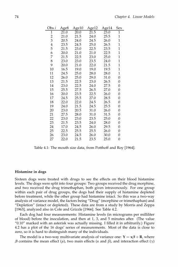
74 Chapter 4. Linear Models
Obs i Age8 Age10 Age12 Age14 Sex1 21.0 20.0 21.5 23.0 12 21.0 21.5 24.0 25.5 13 20.5 24.0 24.5 26.0 14 23.5 24.5 25.0 26.5 15 21.5 23.0 22.5 23.5 16 20.0 21.0 21.0 22.5 17 21.5 22.5 23.0 25.0 18 23.0 23.0 23.5 24.0 19 20.0 21.0 22.0 21.5 110 16.5 19.0 19.0 19.5 111 24.5 25.0 28.0 28.0 112 26.0 25.0 29.0 31.0 013 21.5 22.5 23.0 26.5 014 23.0 22.5 24.0 27.5 015 25.5 27.5 26.5 27.0 016 20.0 23.5 22.5 26.0 017 24.5 25.5 27.0 28.5 018 22.0 22.0 24.5 26.5 019 24.0 21.5 24.5 25.5 020 23.0 20.5 31.0 26.0 021 27.5 28.0 31.0 31.5 022 23.0 23.0 23.5 25.0 023 21.5 23.5 24.0 28.0 024 17.0 24.5 26.0 29.5 025 22.5 25.5 25.5 26.0 026 23.0 24.5 26.0 30.0 027 22.0 21.5 23.5 25.0 0
Table 4.1: The mouth size data, from Potthoff and Roy [1964].
Histamine in dogs
Sixteen dogs were treated with drugs to see the effects on their blood histaminelevels. The dogs were split into four groups: Two groups received the drug morphine,and two received the drug trimethaphan, both given intravenously. For one groupwithin each pair of drug groups, the dogs had their supply of histamine depletedbefore treatment, while the other group had histamine intact. So this was a two-wayanalysis of variance model, the factors being “Drug” (morphine or trimethaphan) and“Depletion” (intact or depleted). These data are from a study by Morris and Zeppa[1963], analyzed also in Cole and Grizzle [1966]. See Table 4.2.
Each dog had four measurements: Histamine levels (in micrograms per milliliterof blood) before the inoculation, and then at 1, 3, and 5 minutes after. (The value“0.10” marked with an asterisk was actually missing. I filled it in arbitrarily.) Figure4.2 has a plot of the 16 dogs’ series of measurements. Most of the data is close tozero, so it is hard to distinguish many of the individuals.
The model is a two-way multivariate analysis of variance one: Y = xβ + R, whereβ contains the mean effect (µ), two main effects (α and β), and interaction effect (γ)
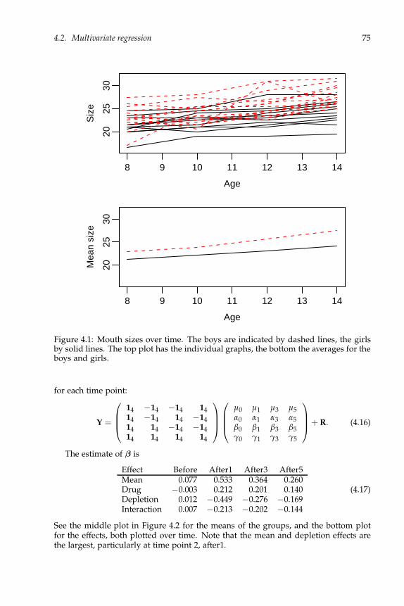
4.2. Multivariate regression 75
8 9 10 11 12 13 14
2025
30
Age
Siz
e
8 9 10 11 12 13 14
2025
30
Age
Mea
n si
ze
Figure 4.1: Mouth sizes over time. The boys are indicated by dashed lines, the girlsby solid lines. The top plot has the individual graphs, the bottom the averages for theboys and girls.
for each time point:
Y =
14 −14 −14 1414 −14 14 −1414 14 −14 −1414 14 14 14
µ0 µ1 µ3 µ5α0 α1 α3 α5β0 β1 β3 β5γ0 γ1 γ3 γ5
+ R. (4.16)
The estimate of β is
Effect Before After1 After3 After5Mean 0.077 0.533 0.364 0.260Drug −0.003 0.212 0.201 0.140Depletion 0.012 −0.449 −0.276 −0.169Interaction 0.007 −0.213 −0.202 −0.144
(4.17)
See the middle plot in Figure 4.2 for the means of the groups, and the bottom plotfor the effects, both plotted over time. Note that the mean and depletion effects arethe largest, particularly at time point 2, after1.

76 Chapter 4. Linear Models
1.0 1.5 2.0 2.5 3.0 3.5 4.0
0.0
1.0
2.0
3.0
Time
His
tam
ine
1.0 1.5 2.0 2.5 3.0 3.5 4.0
0.0
1.0
2.0
3.0
Time
Mea
n hi
stam
ine MI
MDTITD
1.0 1.5 2.0 2.5 3.0 3.5 4.0
−0.
40.
00.
20.
4
Time
Effe
cts
MeanDrugDepletionInteraction
Figure 4.2: Plots of the dogs over time. The top plot has the individual dogs, themiddle plot has the means of the groups, and the bottom plot has the effects in theanalysis of variance. The groups: MI = morphine, intact; MD = morphine, depleted;TI = trimethaphan, intact; TD = trimethaphan, depleted.

4.3. Both sides models 77
Drug×Depletion Obs i Before After1 After3 After5Morphine 1 0.04 0.20 0.10 0.08Intact 2 0.02 0.06 0.02 0.02
3 0.07 1.40 0.48 0.244 0.17 0.57 0.35 0.24
Morphine 5 0.10 0.09 0.13 0.14Depleted 6 0.12 0.11 0.10 ∗0.10
7 0.07 0.07 0.07 0.078 0.05 0.07 0.06 0.07
Trimethaphan 9 0.03 0.62 0.31 0.22Intact 10 0.03 1.05 0.73 0.60
11 0.07 0.83 1.07 0.8012 0.09 3.13 2.06 1.23
Trimethaphan 13 0.10 0.09 0.09 0.08Depleted 14 0.08 0.09 0.09 0.10
15 0.13 0.10 0.12 0.1216 0.06 0.05 0.05 0.05
Table 4.2: The data on histamine levels in dogs. The value with the asterisk is missing,but for illustration purposes I filled it in. The dogs are classified according to thedrug administered (morphine or trimethaphan), and whether the dog’s histaminewas artificially depleted.
4.3 Linear models on both sides
The regression and multivariate regression models in the previous sections modeldifferences between the individuals: The rows of x are different for different indi-viduals, but the same for each variable. Models on the variables switch the roles ofvariable and individual.
4.3.1 One individual
Start with just one individual, so that Y = (Y1, . . . , Yq) is a 1 × q row vector. A linearmodel on the variables is
Y = βz′ + R, where β is 1 × l, R ∼ N1×q(0, ΣR), (4.18)
and z is a fixed q × l matrix. The model (4.18) looks like just a transpose of model(4.1), but (4.18) does not have iid residuals, because the observations are all on thesame individual. Simple repeated measures models and growth curve models are specialcases. (Simple because there is only one individual. Actual models would have morethan one.)
A repeated measure model is used if the Yj’s represent replications of the samemeasurement. E.g., one may measure blood pressure of the same person severaltimes, or take a sample of several leaves from the same tree. If no systematic differ-ences are expected in the measurements, the model would have the same mean µ foreach variable:
Y = µ(1, . . . , 1) + R = µ1′q + R. (4.19)

78 Chapter 4. Linear Models
It is common in this setting to assume ΣR has the intraclass correlation structure, asin (1.61), i.e., the variances are all equal, and the covariances are all equal.
Growth curve models are used when the measurements are made over time, andgrowth (polynomial or otherwise) is expected. A quadratic model turns (4.7) on itsside:
Y = (β0, β1, β2)
1 1 · · · 1x1 x2 · · · xq
x21 x2
2 · · · x2q
+ R. (4.20)
Similarly one can transpose cyclic models akin to (4.8).
4.3.2 IID observations
Now suppose we have a sample of n independent individuals, so that the n × q datamatrix is distributed
Y ∼ Nn×q(1n ⊗µ, In ⊗ ΣR), (4.21)
which is the same as (3.28) with slightly different notation. Here, µ is 1 × q, so themodel says that the rows of Y are independent with the same mean µ and covariancematrix ΣR. The simplest type of a repeated measure model assumes in addition thatthe elements of µ are equal to µ, so that the linear model takes the mean in (4.21) andcombines it with the mean in (4.19) to obtain
Y = 1nµ1′q + R, R ∼ Nn×q(0, In ⊗ ΣR). (4.22)
This model makes sense if one takes a random sample of n individuals, and makesrepeated measurements from each. More generally, a growth curve model as in (4.20),but with n individuals measured, is
Y = 1n(β0, β1, β2)
1 · · · · · · 1z1 z2 · · · zq
z21 z2
2 · · · z2q
+ R. (4.23)
Example: Births
The average births for each hour of the day for four different hospitals is given inTable 4.3. The data matrix Y here is 4 × 24, with the rows representing the hospitalsand the columns the hours. Figure 4.3 plots the curves.
One might wish to fit sine waves (Figure 4.4) to the four hospitals’ data, presumingone day reflects one complete cycle. The model is
Y = βz′ + R, (4.24)
where
β =
β10 β11 β12β20 β21 β22β30 β31 β32β40 β41 β42
(4.25)
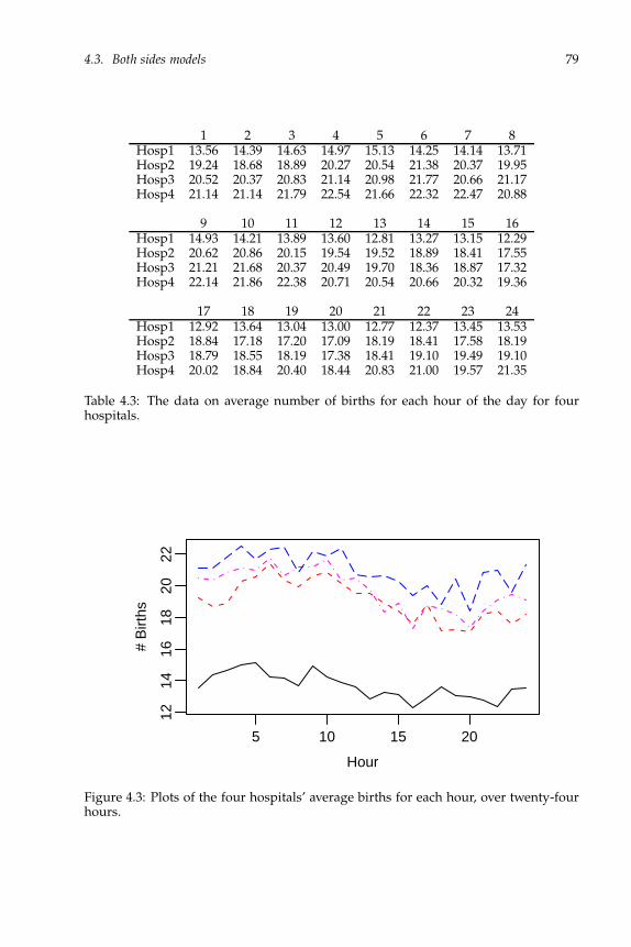
4.3. Both sides models 79
1 2 3 4 5 6 7 8Hosp1 13.56 14.39 14.63 14.97 15.13 14.25 14.14 13.71Hosp2 19.24 18.68 18.89 20.27 20.54 21.38 20.37 19.95Hosp3 20.52 20.37 20.83 21.14 20.98 21.77 20.66 21.17Hosp4 21.14 21.14 21.79 22.54 21.66 22.32 22.47 20.88
9 10 11 12 13 14 15 16Hosp1 14.93 14.21 13.89 13.60 12.81 13.27 13.15 12.29Hosp2 20.62 20.86 20.15 19.54 19.52 18.89 18.41 17.55Hosp3 21.21 21.68 20.37 20.49 19.70 18.36 18.87 17.32Hosp4 22.14 21.86 22.38 20.71 20.54 20.66 20.32 19.36
17 18 19 20 21 22 23 24Hosp1 12.92 13.64 13.04 13.00 12.77 12.37 13.45 13.53Hosp2 18.84 17.18 17.20 17.09 18.19 18.41 17.58 18.19Hosp3 18.79 18.55 18.19 17.38 18.41 19.10 19.49 19.10Hosp4 20.02 18.84 20.40 18.44 20.83 21.00 19.57 21.35
Table 4.3: The data on average number of births for each hour of the day for fourhospitals.
5 10 15 20
1214
1618
2022
Hour
# B
irths
Figure 4.3: Plots of the four hospitals’ average births for each hour, over twenty-fourhours.

80 Chapter 4. Linear Models
0 5 10 15 20
−1.
00.
00.
51.
0
Hour
Sin
e/C
osin
e
Figure 4.4: Sine and cosine waves, where one cycle spans twenty-four hours.
and
z′ =
1 1 · · · 1cos(1 · 2π/24) cos(2 · 2π/24) · · · cos(24 · 2π/24)sin(1 · 2π/24) sin(2 · 2π/24) · · · sin(24 · 2π/24)
, (4.26)
the z here being the same as the x in (4.8).
The estimate of β is
Mean Cosine SineHosp1 13.65 0.03 0.93Hosp2 19.06 −0.69 1.46Hosp3 19.77 −0.22 1.70Hosp4 20.93 −0.12 1.29
(4.27)
Then the “fits” are Y = βz′, which is also 4 × 24. See Figure 4.5.
Now try the model with same curve for each hospital, Y = xβ∗z′ + R, wherex = 14 (the star on the β∗ is to distinguish it from the previous β):
Y = xβ∗z′ + R =
1111
(
β∗0 β∗1 β∗2)
z′ + R. (4.28)
The estimates of the coefficients are now β∗ = (18.35,−0.25, 1.34), which is the aver-
age of the rows of β. The fit is graphed as the thick line in Figure 4.5

4.3. Both sides models 81
5 10 15 20
1214
1618
2022
Hour
# B
irths
Figure 4.5: Plots of the four hospitals’ births, with the fitted sign waves. The thickline fits one curve to all four hospitals.
4.3.3 The both-sides model
Note that the last two models, (4.20) and (4.23), have means with fixed matrices onboth sides of the parameter. Generalizing, we have the model
Y = xβz′ + R, (4.29)
where x is n × p, β is p × l, and z is q × l. The x models differences between indi-viduals, and the z models relationships between the variables. This formulation is byPotthoff and Roy [1964].
For example, consider the mouth size example in Section 4.2. A growth curvemodel seems reasonable, but one would not expect the iid model to hold. In particu-lar, the mouths of the eleven girls would likely be smaller on average than those of thesixteen boys. An analysis of variance model, with two groups, models the differencesbetween the individuals, while a growth curve models the relationship among thefour time points. With Y being the 27 × 4 data matrix of measurements, the model is
Y =
(111 011016 116
)(βg0 βg1 βg2
βb0 βb1 βb2
)
1 1 1 18 10 12 1482 102 122 142
+ R. (4.30)
The “0m”’s are m × 1 vectors of 0’s. Thus (βg0, βg1, βg2) contains the coefficients for
the girls’ growth curve, and (βb0, βb1, βb2) the boys’. Some questions that can beaddressed include
• Does the model fit, or are cubic terms necessary?
• Are the quadratic terms necessary (is βg2 = βb2 = 0)?
• Are the girls’ and boys’ curves the same (are βgj = βbj for j = 0, 1, 2)?

82 Chapter 4. Linear Models
• Are the girls’ and boys’ curves parallel (are βg1 = βb1 and βg2 = βb2, but maybenot βg0 = βb0)?
See also Ware and Bowden [1977] for a circadian application and Zerbe and Jones[1980] for a time-series context. The model is often called the generalized multivari-ate analysis of variance, or GMANOVA, model. Extensions are many. For examples,see Gleser and Olkin [1970], Chinchilli and Elswick [1985], and the book by Kariya[1985].
4.4 Exercises
Exercise 4.4.1 (Prostaglandin). Below are data from Ware and Bowden [1977] taken atsix four-hour intervals (labelled T1 to T6) over the course of a day for 10 individuals.The measurements are prostaglandin contents in their urine.
Person T1 T2 T3 T4 T5 T61 146 280 285 215 218 1612 140 265 289 231 188 693 288 281 271 227 272 1504 121 150 101 139 99 1035 116 132 150 125 100 866 143 172 175 222 180 1267 174 276 317 306 139 1208 177 313 237 135 257 1529 294 193 306 204 207 148
10 76 151 333 144 135 99
(4.31)
(a) Write down the “xβz′" part of the model that fits a separate sine wave to eachperson. (You don’t have to calculate the estimates or anything. Just give the x, β andz matrices.) (b) Do the same but for the model that fits one sine wave to all people.
Exercise 4.4.2 (Skulls). The data concern the sizes of Egyptian skulls over time, fromThomson and Randall-MacIver [1905]. There are 30 skulls from each of five timeperiods, so that n = 150 all together. There are four skull size measurements, all inmillimeters: maximum length, basibregmatic height, basialveolar length, and nasalheight. The model is multivariate regression, where x distinguishes between the timeperiods, and we do not use a z. Use polynomials for the time periods (code them as1, 2, 3, 4, 5), so that x = w ⊗ 130. Find w.
Exercise 4.4.3. Suppose Yb and Ya are n × 1 with n = 4, and consider the model
(Yb Ya) ∼ N(xβ, In ⊗ Σ), (4.32)
where
x =
1 1 11 1 −11 −1 11 −1 −1
. (4.33)
(a) What are the dimensions of β and Σ? The conditional distribution of Ya givenYb = (4, 2, 6, 3)′ is
Ya | Yb = (4, 2, 6, 3)′ ∼ N(x∗β∗, In ⊗ Ω) (4.34)

4.4. Exercises 83
for some fixed matrix x∗, parameter matrix β∗, and covariance matrix Ω. (b) What arethe dimensions of β∗ and Ω? (c) What is x∗? (d) What is the most precise descriptionof the conditional model?
Exercise 4.4.4 (Caffeine). Henson et al. [1996] performed an experiment to see ifcaffeine has a negative effect on short-term visual memory. High school studentswere randomly chosen: 9 from eighth grade, 10 from tenth grade, and 9 from twelfthgrade. Each person was tested once after having caffeinated Coke, and once afterhaving decaffeinated Coke. After each drink, the person was given ten seconds totry to memorize twenty small, common objects, then allowed a minute to write downas many as could be remembered. The main question of interest is whether peopleremembered more objects after the Coke without caffeine than after the Coke withcaffeine. The data are
Grade 8 Grade 10 Grade 12Without With Without With Without With
5 6 6 3 7 79 8 9 11 8 66 5 4 4 9 68 9 7 6 11 77 6 6 8 5 56 6 7 6 9 48 6 6 8 9 76 8 9 8 11 86 7 10 7 10 9
10 6
(4.35)
“Grade" is the grade in school, and the “Without" and “With" entries are the numbersof items remembered after drinking Coke without or with caffeine. Consider themodel
Y = xβz′ + R, (4.36)
where the Y is 28 × 2, the first column being the scores without caffeine, and thesecond being the scores with caffeine. The x is 28 × 3, being a polynomial (quadratic)matrix in the three grades. (a) The z has two columns. The first column of z representsthe overall mean (of the number of objects a person remembers), and the secondcolumn represents the difference between the number of objects remembered withcaffeine and without caffeine. Find z. (b) What is the dimension of β? (c) Whateffects do the βij’s represent? (Choices: overall mean, overall linear effect of grade,overall quadratic effect of grade, overall difference in mean between caffeinated anddecaffeinated coke, linear effect of grade in the difference between caffeinated anddecaffeinated coke, quadratic effect of grade in the difference between caffeinatedand decaffeinated coke, interaction of linear and quadratic effects of grade.)
Exercise 4.4.5 (Histamine in dogs). In Table 4.2, we have the data for the model,
Y = xβz′ + R, (4.37)
where x (n × 4) describes a balanced two-way analysis of variance, as in (4.16). Thecolumns represent, respectively, the overall mean, the drug effect, the depletion effect,and the drug × depletion interaction. For the z, the first column is the effect of the“before” measurement (at time 0), and the last three columns represent polynomial

84 Chapter 4. Linear Models
effects (constant, linear, and quadratic) for just the three “after” time points (times 1,3, 5). (a) What is z? (b) Which of the βij’s represents each of the following effects? (i)Overall drug effect for the after measurements, (ii) overall drug effect for the beforemeasurement, (iii) average after measurement, (iv) drug × depletion interaction forthe before measurement, (v) linear effect in after time points for the drug effect.
Exercise 4.4.6 (Leprosy). Below are data on leprosy patients, found in Snedecor andCochran [1989]. There were 30 patients, randomly allocated to three groups of 10.The first group received drug A, the second drug D, and the third group received aplacebo. Each person had their bacterial count taken before and after receiving thetreatment.
Drug A Drug D PlaceboBefore After Before After Before After
11 6 6 0 16 138 0 6 2 13 105 2 7 3 11 18
14 8 8 1 9 519 11 18 18 21 236 4 8 4 16 12
10 13 19 14 12 56 1 8 9 12 16
11 8 5 1 7 13 0 15 9 12 20
(4.38)
(a) Consider the model Y = xβ + R for the multivariate analysis of variance withthree groups and two variables (so that Y is 30 × 2), where R ∼ N30×2(0, I30 ⊗ ΣR).The x has vectors for the overall mean, the contrast between the drugs and theplacebo, and the contrast between drug A and drug D. Because there are ten peo-ple in each group, x can be written as w ⊗ 110. Find w. (b) Because the beforemeasurements were taken before any treatment, the means for the three groups onthat variable should be the same. Describe that constraint in terms of the β. (c) WithY = (Yb Ya), find the model for the conditional distribution
Ya | Yb = yb ∼ N(x∗β∗, In ⊗ Ω). (4.39)
Give the x∗ in terms of x and yb, and give Ω in terms of the elements of ΣR. (Hint:Write down what it would be with E[Y] = (µb µa) using the conditional formula,then see what you get when µb = xβb and µa = xβa.)
Exercise 4.4.7 (Parity). Johnson and Wichern [2007] present data (in their Exercise6.17) on an experiment. Each of 32 subjects was given several sets of pairs of inte-gers, and had to say whether the two numbers had the same parity (i.e., both odd orboth even), or different parity. So (1, 3) have the same parity, while (4, 5) have dif-ferent parity. Some of the integer pairs were given numerically, like (2, 4), and somewere written out, i.e., (two, f our). The time it took to decide the parity for each pairwas measured. Each person had a little two-way analysis of variance, where the twofactors are parity, with levels different and same, and format, with levels word and nu-meric. The measurements were the median time for each parity/format combinationfor that person. Person i then had observation vector yi = (yi1, yi2, yi3, yi4), which in

4.4. Exercises 85
the ANOVA could be arranged as
FormatParity Word Numeric
Different yi1 yi2Same yi3 yi4
(4.40)
The model is of the formY = xβz′ + R. (4.41)
(a) What are x and z for the model where each person has a possibly differentANOVA, and each ANOVA has effects for overall mean, parity effect, format effect,and parity/format interaction? How many, and which, elements of β must be set tozero to model no-interaction? (b) What are x and z for the model where each personhas the same mean vector, and that vector represents the ANOVA with effects foroverall mean, parity effect, format effect, and parity/format interaction? How many,and which, elements of β must be set to zero to model no-interaction?
Exercise 4.4.8 (Sine waves). Let θ be an angle running from 0 to 2π, so that a sine/-cosine wave with one cycle has the form
g(θ) = A + B cos(θ + C) (4.42)
for parameters A, B, and C. Suppose we observe the wave at the q equally-spacedpoints
θj =2π
qj, j = 1, . . . , q, (4.43)
plus error, so that the model is
Yj = g(θj) + Rj = A + B cos
(2π
qj + C
)+ Rj, j = 1, . . . , q, (4.44)
where the Rj are the residuals. (a) Is the model linear in the parameters A, B, C? Whyor why not? (b) Show that the model can be rewritten as
Yj = β1 + β2 cos
(2π
qj
)+ β3 sin
(2π
qj
)+ Rj, j = 1, . . . , q, (4.45)
and give the βk’s in terms of A, B, C. [Hint: What is cos(a + b)?] (c) Write this modelas a linear model, Y = βz′ + R, where Y is 1 × q. What is the z? (d) Waves withm ≥ 1 cycles can be added to the model by including cosine and sine terms with θreplaced by mθ:
cos
(2πm
qj
), sin
(2πm
qj
). (4.46)
If q = 6, then with the constant term, we can fit in the cosine and sign terms forthe wave with m = 1 cycle, and the cosine and sine terms for the wave with m = 2cycles. The x cannot have more than 6 columns (or else it won’t be invertible). Findthe cosine and sine terms for m = 3. What do you notice? Which one should you putin the model?

Chapter 5
Linear Models: Least Squares and Projections
In this chapter, we briefly review linear subspaces and projections onto them. Most ofthe chapter is abstract, in the sense of not necessarily tied to statistics. The main resultwe need for the rest of the book is the least squares estimate given in Theorem 5.2.Further results can be found in Chapter 1 of Rao [1973], an excellent compendium offacts on linear subspaces and matrices that are useful in statistics.
5.1 Linear subspaces
We start with the space RN . The elements v ∈ RN may be considered row vectors, orcolumn vectors, or matrices, or any other configuration. We will generically call them“vectors.” This space could represent vectors for individuals, in which case N = q,the number of variables, or it could represent vectors for variables, so N = n, thenumber of individuals, or it could represent the entire data matrix, so that N = nq.
A linear subspace is a subset of RN closed under addition and multiplication by ascalar. Because we will deal with Euclidean space, everyone knows what additionand multiplication mean. Here is the definition.
Definition 5.1. A subset W ⊂ RN is a linear subspace of RN if
u, v ∈ W =⇒ u + v ∈ W , and (5.1)
c ∈ R, u ∈ W =⇒ cu ∈ W . (5.2)
We often shorten “linear subspace” to “subspace,” or even “space.” Note that
RN is itself a linear (sub)space, as is the set 0. Because c in (5.2) can be 0, anysubspace must contain 0. Any line through 0, or plane through 0, is a subspace.One convenient representation of subspaces is the set of linear combinations of someelements:
Definition 5.2. The span of the set of vectors d1, . . . , dK ⊂ RN is
spand1, . . . , dK = γ1d1 + · · ·+ γKdK |γ = (γ1, . . . , γK) ∈ RK. (5.3)
By convention, the span of the empty set is just 0. It is not hard to show thatany span is a linear subspace. Some examples: For K = 2, span(1, 1) is the set
87

88 Chapter 5. Least Squares
of vectors of the form (a, a), that is, the equiangular line through 0. For K = 3,span(1, 0, 0), (0, 1, 0) is the set of vectors of the form (a, b, 0), which is the x/yplane, considering the axes to be x, y, z.
We will usually write the span in matrix form. Let D be the N × K matrix withcolumns d1, . . . , dK. We have the following representations of subspace W :
W = spand1, . . . , dK= spancolumns of D= Dγ |γ ∈ RK (γ is K × 1)= spanrows of D′= γD′ |γ ∈ RK (γ is 1 × K). (5.4)
Not only is any span a subspace, but any subspace is a span of some vectors. In
fact, any subspace of RN can be written as a span of at most N vectors, although notnecessarily in a unique way. For example, for N = 3,
span(1, 0, 0), (0, 1, 0) = span(1, 0, 0), (0, 1, 0), (1, 1, 0)= span(1, 0, 0), (1, 1, 0)= span(2, 0, 0), (0,−7, 0), (33, 2, 0). (5.5)
Any invertible transformation of the vectors yields the same span, as in the nextlemma. See Exercise 5.8.4 for the proof.
Lemma 5.1. Suppose W is the span of the columns of the N × K matrix D as in (5.4), andA is an invertible K × K matrix. Then W is also the span of the columns of DA, i.e.,
spancolumns of D = spancolumns of DA. (5.6)
Note that the space in (5.5) can be a span of two or three vectors, or a span of anynumber more than three as well. It cannot be written as a span of only one vector.In the two sets of three vectors, there is a redundancy, that is, one of the vectors canbe written as a linear combination of the other two: (1, 1, 0) = (1, 0, 0) + (0, 1, 0) and
(2, 0, 0) = ( 433×7 (0,−7, 0) + 2
33 × (33, 2, 0). Such sets are called linearly dependent.We first define the opposite.
Definition 5.3. The vectors d1, . . . , dK in RN are linearly independent if
γ1d1 + · · ·+ γKdK = 0 =⇒ γ1 = · · · = γK = 0. (5.7)
The vectors are linearly dependent if and only if they are not linearly indepen-dent. Equivalently, the vectors are linearly dependent if and only if one of them canbe written as a linear combination of the others. That is, they are linearly dependentiff there is a di and set of coefficients γj such that
di = γ1d1 + · · ·+ γi−1di−1 + γi+1di+1 + . . . + γKdK. (5.8)
In (5.5), the sets with three vectors are linearly dependent, and those with twovectors are linearly independent. To see that latter fact for (1, 0, 0), (1, 1, 0), supposethat γ1(1, 0, 0) + γ2(1, 1, 0) = (0, 0, 0). Then
γ1 + γ2 = 0 and γ2 = 0 =⇒ γ1 = γ2 = 0, (5.9)

5.2. Projections 89
which verifies (5.7).If a set of vectors is linearly dependent, then one can remove one of the redundant
vectors (5.8), and still have the same span. A basis is a set of vectors that has the samespan but no dependencies.
Definition 5.4. The set of vectors d1, . . . , dK is a basis for the subspace W if the vectorsare linearly independent and W = spand1, . . . , dK.
Although a (nontrivial) subspace has many bases, each basis has the same numberof elements, which is the dimension. See Exercise 5.8.47.
Definition 5.5. The dimension of a subspace is the number of vectors in any of its bases.
5.2 Projections
In linear models, the mean of the data matrix is presumed to lie in a linear subspace,and an aspect of fitting the model is to find the point in the subspace closest to thedata. This closest point is called the projection. Before we get to the formal definition,we need to define orthogonality. Recall from Section 1.5 that two column vectors vand w are orthogonal if v′w = 0 (or vw′ = 0 if they are row vectors).
Definition 5.6. The vector v ∈ RN is orthogonal to the subspace W ⊂ RN if v is orthogonal
to w for all w ∈ W . Also, subspace V ⊂ RN is orthogonal to W if v and w are orthogonalfor all v ∈ V and w ∈ W .
Geometrically, two objects are orthogonal if they are perpendicular. For example,
in R3, the z-axis is orthogonal to the x/y-plane. Exercise 5.8.6 is to prove the nextresult.
Lemma 5.2. Suppose W = spand1, . . . , dK. Then v is orthogonal to W if and only if vis orthogonal to each dj.
Definition 5.7. The orthogonal projection of v onto W is the v that satisfies
v ∈ W and v − v is orthogonal to W . (5.10)
In statistical parlance, the projection v is the fit and v − v is the residual. Becauseof the orthogonality, we have the decomposition of squared norms,
‖v‖2 = ‖v‖2 + ‖v − v‖2, (5.11)
which is Pythagoras’ Theorem. In a regression setting, the left-hand side is the total
sum-of-squares, and the right-hand side is the regression sum-of-squares (‖v‖2) plus theresidual sum-of-squares, although usually the sample mean of the vi’s is subtractedfrom v and v. See Section 7.2.5.
Because the only projections we will be dealing with directly are orthogonal pro-jections, we will drop the “orthogonal” modifier. So, e.g., the matrix P in part (e) ofthe theorem below is actually the orthogonal projection matrix. Exercises 5.8.8, 5.8.48and 5.8.49 prove the following.
Theorem 5.1 (Projection). Suppose v ∈ RK , W is a subspace of RK , and v is the projectionof v onto W . Then

90 Chapter 5. Least Squares
(a) The projection is unique: If v1 and v2 are both in W , and v − v1 and v − v2 are bothorthogonal to W , then v1 = v2.
(b) If v ∈ W , then v = v.
(c) If v is orthogonal to W , then v = 0.
(d) The projection v uniquely minimizes the Euclidean distance between v and W , that is,
‖v − v‖2< ‖v − w‖2 for all w ∈ W , w 6= v. (5.12)
(e) There exists a unique N × N matrix P, called the projection matrix, such that
vP = v for all v ∈ RN . (5.13)
The final equation is assuming v is a row vector. If it is a column vector, then wehave Pv = v. We present an explicit formula for the projection matrix in (5.20).
5.3 Least squares
In this section, we explicitly find the projection of v (1 × N) onto W . Supposed1, . . . , dK, the columns of the N × K matrix D, form a basis for W , so that the fi-nal expression in (5.4) holds. Consider the linear model
V = γD′ + R, (5.14)
where γ is 1 × K. Our objective is to find a vector γ so that v ≈ γD′. One approachis least squares.
Definition 5.8. A least squares estimate of γ in the equation (5.14) is any γ such that
‖v − γD′‖2 = minγ∈RK
‖v − γD′‖2. (5.15)
Part (d) of Theorem 5.1 implies that a least squares estimate of γ is any γ forwhich γD′ is the projection of v onto the subspace W . Thus v − γD′ is orthogonalto W , and by Lemma 5.2, is orthogonal to each dj. These orthogonality conditionsresult in the normal equations:
(v − γD′)dj = 0 for each j = 1, . . . , K. (5.16)
We then have
(5.16) =⇒ (v − γD′)D = 0
=⇒ γD′D = vD (5.17)
=⇒ γ = vD(D′D)−1, (5.18)
where the final equation holds if D′D is invertible, which occurs if and only if thecolumns of D constitute a basis of W . See Exercise 5.8.46. (If D′D is not invertible,then we can substitute its Moore-Penrose inverse for (D′D)−1 in (5.18) to obtain oneof the solutions to (5.17). See Exercise 3.7.24.) Summarizing:

5.4. Best linear unbiased estimators 91
Theorem 5.2 (Least squares). Any solution γ to the least squares equation (5.15) satisfiesthe normal equations (5.17). The solution is unique if and only if D′D is invertible, in whichcase (5.18) holds.
If D′D is invertible, the projection of v onto W can be written
v = γD′ = vD(D′D)−1D′ ≡ vPD, (5.19)
wherePD = D(D′D)−1D′ (5.20)
is the projection matrix for W as in part (e) of Theorem 5.1. The residual vector isthen
v − v = v − vPD = v(IN − PD) = vQD, (5.21)
whereQD = IN − PD. (5.22)
The minimum value in (5.15) can be written
‖v − v‖2 = vQDv′. (5.23)
Exercises 5.8.12 to 5.8.14 prove the following properties of projection matrices.
Proposition 5.1 (Projection matrices). Suppose PD is defined as in (5.20), where D′D isinvertible. Then the following hold.
(a) PD is symmetric and idempotent, with trace(PD) = K, the dimension of W ;
(b) Any symmetric idempotent matrix is a projection matrix for some subspace W ;
(c) QD = IN − PD is also a projection matrix, and is orthogonal to PD in the sense thatPDQD = QDPD = 0;
(d) PDD = D and QDD = 0.
The matrix QD is the projection matrix onto the orthogonal complement of W ,
where the orthogonal complement contains all vectors in RN that are orthogonal toW .
5.4 Best linear unbiased estimators
One might wonder whether the least squares estimate is a good one. We add momentconditions on R to the model in (5.14):
V = γD′ + R, where E[R] = 0 and Cov[R] = Ω. (5.24)
We also assume that D′D is invertible. The goal in this section is to find the “bestlinear unbiased estimator” of γ.
An estimator γ is linear in v ifγ = vL (5.25)
for some N × K constant matrix L. Because (5.24) implies that E[V] = γD′, theestimator (5.25) is unbiased if and only if
E[γ] = γD′L = γ for all γ ∈ RK ⇐⇒ D′L = IK. (5.26)

92 Chapter 5. Least Squares
(See Exercise 5.8.17.) From (5.18), the least squares estimator is linear,
γLS = vLLS with LLS = D(D′D)−1, (5.27)
and because D′LLS = D′D(D′D)−1 = IK as in (5.26), the estimator is unbiased.We are interested in finding the linear unbiased estimator with the smallest co-
variance matrix. In general, Cov[VL] = L′ΩL, but we will initially assume that Ω is
the identity matrix, so that
Ω = IN =⇒ Cov[VL] = L′L and Cov[VLLS] = L′LSLLS = (D′D)−1. (5.28)
The main result is next.
Theorem 5.3. Gauss-Markov Theorem. In model (5.24) with Ω = IN , the least squaresestimator γLS is the best linear unbiased estimator (BLUE) of γ in the sense that it islinear and unbiased, and for any other linear unbiased estimator γ = vL,
Cov[γ]− Cov[γLS] is nonnegative definite. (5.29)
Proof. Let M = L − LLS. Then by (5.26) and assumption of unbiasedness,
IK = D′L = D′(LLS + M) = D′LLS + D′M = IK + D′M, (5.30)
hence D′M = 0. Then
Cov[VL] = (LLS + M)′(LLS + M)
= L′LSLLS + M′M + L′
LSM + M′LLS
= Cov[VLLS] + M′M, (5.31)
sinceL′
LSM = (D′D)−1D′M = 0. (5.32)
The matrix M′M is nonnegative definite, hence we have (5.29).
The conclusion in the theorem means that for any linear combination γa, where ais K × 1,
Var[γa] ≥ Var[γLSa], (5.33)
so that the least squares estimate has the lowest variance of any linear unbiasedestimator. In particular, it is best for each component of γi.
Theorem 5.3 holds also if Cov[R] = σ2IN for scalar σ2> 0 in (5.24), but not
necessarily for Cov[R] = Ω for arbitrary positive definite Ω. But it is easy to rewritethe model to find the BLUE. Let
V∗ = VΩ- ½, D∗ = Ω
- ½D, R∗ = RΩ- ½. (5.34)
Then we have the situation in (5.24), where V∗ = γD∗′ + R∗ and Cov[R∗] = IN . Thusthe least squares estimate in this new model is BLUE, where here
γWLS = v∗D∗(D∗′D∗)−1
= vΩ−1D(D′
Ω−1D)−1. (5.35)
5.5. Least squares in the both-sides model 93
The “WLS” in the subscript of the estimator stands for “weighted least squares,”because this estimator minimizes the weighted objective function
(v − γD′)Ω−1(v − γD′)′. (5.36)
See Exercise 5.8.18. The covariance matrix for the BLUE in (5.35) is by (5.28)
Cov[γWLS] = (D∗′D∗)−1
= (D′Ω
−1D)−1. (5.37)
5.5 Least squares in the both-sides model
We now specialize to the both-sides model as defined in (4.29), i.e.,
Y = xβz′ + R, R ∼ N(0, In ⊗ ΣR), (5.38)
where Y is n × q, x is n × p, β is p × l, and z is q × l. We assume x′x, z′z, and ΣRare invertible. In order to find the best linear unbiased estimator of β, we make thefollowing identifications between (5.24) and (5.38):
V = row(Y), γ = row(β), D = x ⊗ z, Ω = In ⊗ ΣR. (5.39)
Also, in (5.24), R is 1 × N, while in (5.38), it is n × q.Theorem 5.3 shows that the BLUE of β, assuming ΣR is known, is the weighted
least squares estimate in (5.35). Using Proposition 3.2, we translate the formula to
row(β)WLS = vΩ−1D(D′
Ω−1D)−1
= row(y)(In ⊗ ΣR)−1(x ⊗ z)((x ⊗ z)′(In ⊗ ΣR)
−1(x ⊗ z))−1
= row(y)(x ⊗ Σ−1R z)(x′x ⊗ z′Σ−1
R z)−1
= row(y)(x(x′x)−1 ⊗ Σ−1R z(z′Σ−1
R z)−1). (5.40)
Thus, unrowing,
βWLS = (x′x)−1x′yΣ−1R z(z′Σ−1
R z)−1. (5.41)
By (5.37),
Cov[βWLS] = ((x ⊗ z)′(In ⊗ ΣR)−1(x ⊗ z))−1
= (x′x)−1 ⊗ (z′Σ−1R z)−1. (5.42)
Because ΣR is typically not known, its presence in the estimator of β can be prob-lematic. Thus we often instead use the unweighted least squares estimator, which isas in (5.41) but with Iq instead of ΣR:
βLS = (x′x)−1x′Yz(z′z)−1. (5.43)
This estimator is not necessarily BLUE. By (3.34), its covariance is
Cov[βLS] = (D′D)−1D′ΩD(D′D)−1
= ((x′x)−1x′)((x′x)−1x′)′ ⊗ (z(z′z)−1)′ΣRz(z′z)−1
= Cx ⊗ Σz, (5.44)

94 Chapter 5. Least Squares
where we define
Cx = (x′x)−1and Σz = (z′z)−1z′ΣRz(z′z)−1. (5.45)
But in the multivariate regression case (4.9), where z = Iq, or in fact whenever z
is square (hence invertible, since z′z is assumed invertible), the dependence on ΣRdisappears:
z is q × q =⇒ βWLS = (x′x)−1x′yΣ−1R z(Σ−1
R z)−1(z′)−1
= (x′x)−1x′y(z′)−1
= βLS. (5.46)
Chapter 6 treats estimation of ΣR and standard errors of the βij’s for the leastsquares estimator. Consideration of the weighted least squares estimator appears inSection 9.3.1 on maximum likelihood estimates.
5.6 What is a linear model?
We have been working with linear models for a while, so perhaps it is time to formallydefine them. Basically, a linear model for Y is one for which the mean of Y lies in agiven linear subspace. A model itself is a set of distributions. The linear model doesnot describe the entire distribution, thus the actual distribution, e.g., multivariatenormal with a particular covariance structure, needs to be specified as well. In theboth-sides model (6.1), with the identifications in (5.39), we have
E[row(Y)] = row(β)(x ⊗ z)′. (5.47)
Letting β range over all the p × l matrices, we have the restriction
E[row(Y)] ∈ W ≡ row(β)(x ⊗ z)′ | row(β) ∈ Rpl. (5.48)
Is W a linear subspace? Indeed, as in Definition 5.2, it is the span of the columnsof x ⊗ z, the columns being xi ⊗ zj, where xi and zj are the columns of x and z,respectively. That is,
row(β)(x ⊗ z)′ =p
∑i=1
l
∑j=1
βij(xi ⊗ zj)′. (5.49)
The linear model is then the set of distributions
M = N(M, In ⊗ ΣR) | M ∈ W and ΣR ∈ S+q , (5.50)
denoting
S+q = The set of q × q positive definite symmetric matrices. (5.51)
Other linear models can have different distributional assumptions, e.g., covariancerestrictions, but do have to have the mean lie in a linear subspace.

5.7. Gram-Schmidt orthogonalization 95
There are many different parametrizations of a given linear model, for the samereason that there are many different bases for the mean space W . For example, itmay not be obvious, but
x =
(1 00 1
), z =
1 1 11 2 41 3 9
(5.52)
and
x∗ =
(1 −11 1
), z∗ =
1 −1 11 0 −21 1 1
(5.53)
lead to exactly the same model, though different interpretations of the parameters.In fact, with x being n × p and z being q × l,
x∗ = xA and z∗ = zB (5.54)
yields the same model as long as A (p × p) and B (l × l) are invertible:
xβz′ = x∗β∗z∗′ with β∗ = A−1β(B′)−1. (5.55)
The representation in (5.53) has the advantage that the columns of the x∗ ⊗ z∗ areorthogonal, which makes it easy to find the least squares estimates as the D′D matrixis diagonal, hence easy to invert. Note the z is the matrix for a quadratic. The z∗ isthe corresponding set of orthogonal polynomials, as discussed in Section 5.7.2.
5.7 Gram-Schmidt orthogonalization
We have seen polynomial models in (4.7), (4.23), and (4.30). Note that, especiallyin the latter case, one can have a design matrix (x or z) whose entries have widelyvarying magnitudes, as well as highly correlated column vectors, which can lead tonumerical difficulties in calculation. Orthogonalizing the vectors, without changingtheir span, can help both numerically and for interpretation. Gram-Schmidt orthogo-nalization is a well-known constructive approach. It is based on the following lemma.
Lemma 5.3. Suppose (D1, D2) is N × K, where D1 is N × K1, D2 is N × K2, and W isthe span of the combined columns:
W = spancolumns of (D1, D2). (5.56)
Suppose D′1D1 is invertible, and let
D2·1 = QD1D2, (5.57)
for QD1defined in (5.22) and (5.20). Then the columns of D1 and D2·1 are orthogonal,
D′2·1D1 = 0, (5.58)
and
W = spancolumns of (D1, D2·1). (5.59)

96 Chapter 5. Least Squares
Proof. D2·1 is the residual matrix for the least squares model D2 = D1β + R, i.e., D1is the x and D2 is the Y in the multivariate regression model (4.9). Equation (5.58)then follows from part (d) of Proposition 5.1: D′
2·1D1 = D′2QD1
D1 = 0. For (5.59),
(D1 D2·1
)=(
D1 D2
) ( IK1−(D′
1D1)−1D′
1D20 IK2
). (5.60)
The final matrix is invertible, hence by Lemma 5.1, the spans of the columns of(D1, D2) and (D1, D2·1) are the same.
Now let d1, . . . dK be the columns of the N × K matrix D, and W their span.The Gram-Schmidt process starts by applying Lemma 5.3 with D1 = d1 and D2 =(d2, . . . , dK). Write the resulting columns of D2·1 as the vectors
d2·1, · · · , dK·1, where dj·1 = dj −d′
jd1
‖d1‖2d1. (5.61)
In other words, dj·1 is the residual of the projection of dj onto spand1. Thus d1 is
orthogonal to all the dj·1’s in (5.61), and W = spand1, d2·1, . . . , dK·1 by (5.59).Second step is to apply the lemma again, this time with D1 = d2·1, and D2 =
(d3·1, . . . , dK·1), leaving aside the d1 for the time being. Now write the columns ofthe new D2·1 dotting out the “1” and “2”:
d3·12, · · · , dK·12, where dj·12 = dj·1 −d′
j·1d2·1‖d2·1‖2
d2·1. (5.62)
Now d2·1, as well as d1, are orthogonal to the vectors in (5.62), and
W = spand1, d2·1, d3·12, . . . , dK·12. (5.63)
We continue until we have the set of vectors
d1, d2·1, d3·12, . . . , dK·1:(K−1), (5.64)
which are mutually orthogonal and span W . Here, we are using the R-based notation
a : b = a, a + 1, . . . , b for integers a < b. (5.65)
It is possible that one or more of the vectors we use for D1 will be zero. In suchcases, we just leave the vectors in D2 alone, i.e., D2·1 = D2, because the projectionof any vector on the space 0 is 0, hence the residual equals the original vector.We can describe the entire resulting process iteratively, for i = 1, . . . , K − 1 and j =i + 1, . . . , K, as setting
dj·1:i = dj·1:(i−1)− γij di·1:(i−1), (5.66)
where
γij =d′
j·1:(i−1)di·1:(i−1)‖di·1:(i−1)‖2
(5.67)
if its denominator is nonzero. Otherwise, set γij = 0, although any value will do.

5.7. Gram-Schmidt orthogonalization 97
Optionally, one can multiply any of these vectors by a nonzero constant, e.g., sothat it has a norm of one, or for esthetics, so that the entries are small integers. Anyzero vectors left in the set can be eliminated without affecting the span.
Note that by the stepwise nature of the algorithm, we have that the spans of thefirst k vectors from each set are equal, that is,
spand1, d2 = spand1, d2·1spand1, d2, d3 = spand1, d2·1, d3·12
...
spand1, d2, . . . , dK = spand1, d2·1, d3·12, . . . , dK·1:(K−1). (5.68)
The next section derives some important matrix decompositions based on theGram-Schmidt orthogonalization. Section 5.7.2 applies the orthogonalization to poly-nomials.
5.7.1 The QR and Cholesky decompositions
We can write the Gram-Schmidt process in matrix form. The first step is
(d1 d2·1 · · · dK·1
)= D
1 −γ12 · · · −γ1K0 1 · · · 0...
.... . .
...0 0 · · · 1
. (5.69)
The γij’s are defined in (5.67). Next,
(d1 d2·1 d3·12 · · · dK·12
)
=(
d1 d2·1 · · · dK·1)
1 0 0 · · · 00 1 −γ23 · · · −γ2K0 0 1 · · · 0...
......
. . ....
0 0 0 · · · 1
. (5.70)
We continue, so that the final result is
D∗ ≡(
d1 d2·1 d3·12 · · · dK·1:(K−1))= DB(1)B(2) · · · B(K−1), (5.71)
where B(k) is the identity except for the elements kj, j > k:
B(k)ij =
1 if i = j
−γkj if j > k = i
0 otherwise.
(5.72)
These matrices are upper unitriangular, meaning they are upper triangular (i.e.,all elements below the diagonal are zero), and all diagonal elements are one. We willuse the notation
T 1q = T | T is q × q, tii = 1 for all i, tij = 0 for i > j. (5.73)
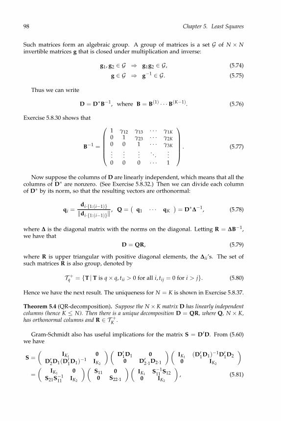
98 Chapter 5. Least Squares
Such matrices form an algebraic group. A group of matrices is a set G of N × Ninvertible matrices g that is closed under multiplication and inverse:
g1, g2 ∈ G ⇒ g1g2 ∈ G , (5.74)
g ∈ G ⇒ g−1 ∈ G . (5.75)
Thus we can write
D = D∗B−1, where B = B(1) · · · B(K−1). (5.76)
Exercise 5.8.30 shows that
B−1 =
1 γ12 γ13 · · · γ1K0 1 γ23 · · · γ2K0 0 1 · · · γ3K...
......
. . ....
0 0 0 · · · 1
. (5.77)
Now suppose the columns of D are linearly independent, which means that all thecolumns of D∗ are nonzero. (See Exercise 5.8.32.) Then we can divide each columnof D∗ by its norm, so that the resulting vectors are orthonormal:
qi =di·1:(i−1)
‖di·1:(i−1)‖, Q =
(q1 · · · qK
)= D∗
∆−1, (5.78)
where ∆ is the diagonal matrix with the norms on the diagonal. Letting R = ∆B−1,we have that
D = QR, (5.79)
where R is upper triangular with positive diagonal elements, the ∆ii’s. The set ofsuch matrices R is also group, denoted by
T +q = T | T is q × q, tii > 0 for all i, tij = 0 for i > j. (5.80)
Hence we have the next result. The uniqueness for N = K is shown in Exercise 5.8.37.
Theorem 5.4 (QR-decomposition). Suppose the N × K matrix D has linearly independentcolumns (hence K ≤ N). Then there is a unique decomposition D = QR, where Q, N × K,has orthonormal columns and R ∈ T +
K .
Gram-Schmidt also has useful implications for the matrix S = D′D. From (5.60)we have
S =
(IK1
0
D′2D1(D
′1D1)
−1 IK2
)(D′
1D1 00 D′
2·1D2·1
)(IK1
(D′1D1)
−1D′1D2
0 IK2
)
=
(IK1
0
S21S−111 IK2
)(S11 00 S22·1
)(IK1
S−111 S12
0 IK2
), (5.81)

5.7. Gram-Schmidt orthogonalization 99
where S22·1 = S22 − S21S−111 S12 as in (3.49). See Exercise 5.8.38. Then using steps as
in Gram-Schmidt, we have
S = (B−1)′
S11 0 0 · · · 00 S22·1 0 · · · 00 0 S33·12 · · · 0...
......
. . ....
0 0 0 · · · SKK·1:(K−1)
B−1
= R′R, (5.82)
because the inner matrix is ∆2. Also, note that
γij = Sij·1:(i−1)/Sii·1:(i−1) for j > i, (5.83)
and R is given by
Rij =
√Sii·1:(i−1) if j = i,
Sij·1:(i−1)/√
Sii·1:(i−1) if j > i,
0 if j < i.
(5.84)
Exercise 5.8.43 shows this decomposition works for any positive definite symmetricmatrix. It is then called the Cholesky decomposition:
Theorem 5.5 (Cholesky decomposition). If S ∈ S+q (5.51), then there exists a unique
R ∈ T +q such that S = R′R.
Note that this decomposition yields a particular square root of S.
5.7.2 Orthogonal polynomials
Turn to polynomials. We will illustrate with the example on mouth sizes in (4.30).Here K = 4, and we will consider the cubic model, so that the vectors are
(d1 d2 d3 d4
)=
1 8 82 83
1 10 102 103
1 12 122 123
1 14 142 143
. (5.85)
Note that the ages (values 8, 10, 12, 14) are equally spaced. Thus we can just as wellcode the ages as (0,1,2,3), so that we actually start with
(d1 d2 d3 d4
)=
1 0 0 01 1 1 11 2 4 81 3 9 27
. (5.86)

100 Chapter 5. Least Squares
Dotting d1 out of vector w is equivalent to subtracting the mean of the elementsof w for each element. Hence
d2·1 =
−3/2−1/2
1/23/2
→
−3−1
13
, d3·1 =
−7/2−5/2
1/211/2
→
−7−5
111
, d4·1 =
−9−8−118
.
(5.87)
We multiplied the first two vectors in (5.87) by 2 for simplicity. Next, we dot d2·1 outof the last two vectors. So for d3·1, we have
d3·12 =
−7−5
111
− (−7,−5, 1, 11)(−3,−1, 1, 3)′
‖(−3,−1, 1, 3)‖2
−3−1
13
=
2−2−2
2
→
1−1−1
1
(5.88)and, similarly, d4·12 = (4.2,−3.6,−5.4, 4.8)′ → (7,−6,−9, 8)′. Finally, we dot d3·12out of d4·12 to obtain d4·123 = (−1, 3,−3, 1)′. Then our final orthogonal polynomialmatrix is the very nice
(d1 d2·1 d3·12 d4·123
)=
1 −3 1 −11 −1 −1 31 1 −1 −31 3 1 1
. (5.89)
Some older statistics books (e.g., Snedecor and Cochran [1989]) contain tables of or-thogonal polynomials for small K, and statistical packages will calculate them foryou. In R, the function is poly.
A key advantage to using orthogonal polynomials over the original polynomialvectors is that, by virtue of the sequence in (5.68), one can estimate the parametersfor models of all degrees at once. For example, consider the mean of the girls’ mouthsizes in (4.15) as the V, and the matrix in (5.89) as the D, in the model (5.24):
(21.18, 22.23, 23.09, 24.09) ≈ (γ1, γ2, γ3, γ4)
1 1 1 1−3 −1 1 3
1 −1 −1 1−1 3 −3 1
. (5.90)
Because D′D is diagonal, the least squares estimates of the coefficients are found via
γj =vdj·1:(j−1)‖dj·1:(j−1)‖2
, (5.91)
which here yields
γ = (22.6475, 0.4795, −0.0125, 0.0165). (5.92)
These are the coefficients for the cubic model. The coefficients for the quadratic modelset γ4 = 0, but the other three are as for the cubic. Likewise, the linear model has γequalling (22.6475, 0.4795, 0, 0), and the constant model has (22.6475, 0, 0, 0).

5.8. Exercises 101
In contrast, if one uses the original vectors in either (5.85) or (5.86), one has to recal-culate the coefficients separately for each model. Using (5.86), we have the followingestimates:
Model γ∗1 γ∗
2 γ∗3 γ∗
4Cubic 21.1800 1.2550 −0.2600 0.0550Quadratic 21.1965 0.9965 −0.0125 0Linear 21.2090 0.9590 0 0Constant 22.6475 0 0 0
(5.93)
Note that the nonzero values in each column are not equal.
5.8 Exercises
Exercise 5.8.1. Show that the span in (5.3) is indeed a linear subspace.
Exercise 5.8.2. Verify that the four spans given in (5.5) are the same.
Exercise 5.8.3. Show that for matrices C (N × J) and D (N × K),
spancolumns of D ⊂ spancolumns of C ⇒ D = CA, (5.94)
for some J × K matrix A. [Hint: Each column of D must be a linear combination ofthe columns of C.]
Exercise 5.8.4. Here, D is an N × K matrix, and A is K × L. (a) Show that
spancolumns of DA ⊂ spancolumns of D. (5.95)
[Hint: Any vector in the left-hand space equals DAγ for some L × 1 vector γ. Forwhat vector γ∗ is DAγ = Dγ∗?] (b) Prove Lemma 5.1. [Use part (a) twice, once for
A and once for A−1.] (c) Show that if the columns of D are linearly independent,and A is K × K and invertible, then the columns of DA are linearly independent.[Hint: Suppose the columns of DA are linearly dependent, so that for some γ 6= 0,DAγ = 0. Then there is a γ∗ 6= 0 with Dγ∗ = 0. What is it?]
Exercise 5.8.5. Let d1, . . . , dK be vectors in RN . (a) Suppose (5.8) holds. Show thatthe vectors are linearly dependent. [That is, find γj’s, not all zero, so that ∑ γidi = 0.](b) Suppose the vectors are linearly dependent. Find an index i and constants γj sothat (5.8) holds.
Exercise 5.8.6. Prove Lemma 5.2.
Exercise 5.8.7. Suppose the set of M × 1 vectors g1, . . . , gK are nonzero and mutuallyorthogonal. Show that they are linearly independent. [Hint: Suppose they are linearlydependent, and let gi be the vector on the left-hand side in (5.8). Then take g′
i timeseach side of the equation, to arrive at a contradiction.]
Exercise 5.8.8. Prove part (a) of Theorem 5.1. [Hint: Show that the difference of v− v1and v − v2 is orthogonal to W , as well as in W . Then show that such a vector must bezero.] (b) Prove part (b) of Theorem 5.1. (c) Prove part (c) of Theorem 5.1. (d) Prove
part (d) of Theorem 5.1. [Hint: Start by writing ‖v − w‖2 = ‖(v − v)− (w − v)‖2,then expand. Explain why v − v and w − v are orthogonal.]
102 Chapter 5. Least Squares
Exercise 5.8.9. Suppose D1 is N × K1, D2 is N × K2, and D′1D2 = 0. Let Vi =
spancolumns of Di for i = 1, 2. (a) Show that V1 and V2 are orthogonal spaces. (b)Define W = spancolumns of (D1, D2). (The subspace W is called the direct sumof the subspaces V1 and V2.) Show that u is orthogonal to V1 and V2 if and only if it
is orthogonal to W . (c) For v ∈ RN , let vi be the projection onto Vi, i = 1, 2. Showthat v1 + v2 is the projection of v onto W . [Hint: Show that v − v1 − v2 is orthogonalto V1 and V2, then use part (b).]
Exercise 5.8.10. Derive the normal equations (5.16) by differentiating ‖v − γD′‖2
with respect to the γi’s.
Exercise 5.8.11. Suppose A and B are both n × q matrices. Exercise 3.7.6 showed thattrace(AB′) = trace(B′A). Show further that
trace(AB′) = trace(B′A) = row(A) row(B)′. (5.96)
Exercise 5.8.12. This exercise proves part (a) of Proposition 5.1. Suppose W =spancolumns of D, where D is N × K and D′D is invertible. (a) Show that the
projection matrix PD = D(D′D)−1D′ as in (5.20) is symmetric and idempotent. (b)Show that trace(PD) = K. [Use Exercise 5.8.11.]
Exercise 5.8.13. This exercise proves part (b) of Proposition 5.1. Suppose P is a sym-metric and idempotent N × N matrix. Find a set of linearly independent vectorsd1, . . . , dK, where K = trace(P), so that spand1, . . . , dK has projection matrix P.[Hint: Write P = Γ1Γ
′1 where Γ1 has orthonormal columns, as in Lemma 3.1. Show
that P is the projection matrix onto the span of the columns of the Γ1, and use Exercise5.8.7 to show that those columns are a basis. What is D, then?]
Exercise 5.8.14. (a) Prove part (c) of Proposition 5.1. (b) Prove part (d) of Proposition5.1. (c) Prove (5.23).
Exercise 5.8.15. Consider the projection of v ∈ RN onto span1′N. (a) Find theprojection. (b) Find the residual. What does it contain? (c) Find the projection matrixP. What is Q = IN − P? Have we seen it before?
Exercise 5.8.16. Suppose D is N × K and D∗ is N × L, where spancolumns of D ⊂spancolumns of D∗. (a) Show that PDPD∗ = PD∗PD = PD. [Hint: What is PD∗D?](b) Show that QDQD∗ = QD∗QD = QD∗ .
Exercise 5.8.17. Suppose A is a K × K matrix such that γA = γ for all 1 × K vectorsγ. Show that A = IK.
Exercise 5.8.18. Show that the quadratic form in (5.36) equals ‖v∗ − γD∗′‖2 for v∗
and D∗ in (5.34). Conclude that the weighted least squares estimator (5.35) doesminimize (5.34).
Exercise 5.8.19. Show that the weighted least squares estimate (5.35) is the same as
the regular least squares estimate (5.18) when in (5.24) the covariance Ω = σ2IN for
some σ2> 0.
Exercise 5.8.20. Verify the steps in (5.40), (5.41), and (5.42), detailing which parts ofProposition 3.2 are used at each step.
Exercise 5.8.21. Verify (5.44).
5.8. Exercises 103
Exercise 5.8.22. Verify (5.60).
Exercise 5.8.23. Show that for any K1 × K2 matrix A,
(IK1
A0 IK2
)−1
=
(IK1
−A0 IK2
). (5.97)
Exercise 5.8.24. Suppose D = (D1, D2), where D1 is N × K1, D2 is N × K2, andD′
1D2 = 0. Use Exercise 5.8.9 to show that PD = PD1+ PD2
.
Exercise 5.8.25. Suppose D = (D1, D2), where D1 is N × K1, D2 is N × K2 (butD′
1D2 6= 0, maybe). (a) Use Exercise 5.8.24 and Lemma 5.3 to show that PD =PD1
+ PD2·1 , where D2·1 = QD1D2 as in (5.57). (b) Show that QD1
= QD + PD2·1 .
Exercise 5.8.26. Show that the equation for dj·1 in (5.61) does follow from the deriva-tion of D2·1.
Exercise 5.8.27. Give an argument for why the set of equations in (5.68) follows fromthe Gram-Schmidt algorithm.
Exercise 5.8.28. Given that a subspace is a span of a set of vectors, explain how onewould obtain an orthogonal basis for the space.
Exercise 5.8.29. Let Z1 be a N × K matrix with linearly independent columns. (a)How would you find a N × (N − K) matrix Z2 so that (Z1, Z2) is an invertible N × Nmatrix, and Z′
1Z2 = 0 (i.e., the columns of Z1 are orthogonal to those of Z2). [Hint:Start by using Lemma 5.3 with D1 = Z1 and D2 = IN . (What is the span of thecolumns of (Z1, IN)?) Then use either Gram-Schmidt or Exercise 5.8.13 on D2·1 tofind a set of vectors to use as the Z2. Do you recognize D2·1?] (b) Suppose thecolumns of Z1 are orthonormal. How would you modify the Z2 obtained in part (a)so that (Z1, Z2) is an orthogonal matrix?
Exercise 5.8.30. Consider the matrix B(k) defined in (5.72). (a) Use Exercise 5.8.23 to
show that the inverse of B(k) is of the same form, but with the −bkj’s changed to bkj’s.
That is, the inverse is the K × K matrix C(k), where
C(k)ij =
1 if i = j
bkj if j > k = i
0 otherwise.
(5.98)
Thus C is the inverse of the B in (5.76), where C = C(K−1) · · · C(1). (b) Show thatC is unitriangular, where the bij’s are in the upper triangular part, i.e, Cij = bij forj > i, as in (5.77). (c) The R in (5.79) is then ∆C, where ∆ is the diagonal matrix withdiagonal elements being the norms of the columns of D∗. Show that R is given by
Rij =
‖di·1:(i−1)‖ if j = i
d′j·1:(i−1)di·1:(i−1)/‖di·1:(i−1)‖ if j > i
0 if j < i.
(5.99)
Exercise 5.8.31. Verify (5.83).
104 Chapter 5. Least Squares
Exercise 5.8.32. Suppose d1, . . . , dK are vectors in RN , and d∗1 , . . . , d∗
K are the corre-sponding orthogonal vectors resulting from the Gram-Schmidt algorithm, i.e., d∗
1 =d1, and for i > 1, d∗
i = di·1:(i−1) in (5.66). (a) Show that the d∗1 , . . . , d∗
K are linearly
independent if and only if they are all nonzero. Why? [Hint: Recall Exercise 5.8.7.](b) Show that d1, . . . , dK are linearly independent if and only if all the d∗
j are nonzero.
Exercise 5.8.33. Suppose D is N × K, with linearly independent columns, and D =QR is its QR decomposition. Show that spancolumns of D = spancolumns of Q.
Exercise 5.8.34. Suppose D is an N × N matrix whose columns are linearly indepen-dent. Show that D is invertible. [Hint: Use the QR decomposition in Theorem 5.4.What kind of a matrix is the Q here? Is it invertible?]
Exercise 5.8.35. (a) Show that spancolumns of Q = RN if Q is an N × N orthogonalmatrix. (b) Suppose the N × 1 vectors d1, . . . , dN are linearly independent, and W =spand1, . . . , dN. Show that W = RN . [Hint: Use Theorem 5.4, Lemma 5.1, and part(a).]
Exercise 5.8.36. Show that if d1, . . . , dK are vectors in RN with K > N, that the di’sare linearly dependent. (This fact should make sense, since there cannot be more axesthan there are dimensions in Euclidean space.) [Hint: Use Exercise 5.8.35 on the firstN vectors, then show how dN+1 is a linear combination of them.]
Exercise 5.8.37. Show that the QR decomposition in Theorem 5.4 is unique whenN = K. That is, suppose Q1 and Q2 are K × K orthogonal matrices, and R1 andR2 are K × K upper triangular matrices with positive diagonals, and Q1R1 = Q2R2.
Show that Q1 = Q2 and R1 = R2. [Hint: Show that Q ≡ Q′2Q1 = R2R−1
1 ≡ R,so that the orthogonal matrix Q equals the upper triangular matrix R with positivediagonals. Show that therefore Q = R = IK .] [Extra credit: Show the uniquenesswhen M > K.]
Exercise 5.8.38. Verify (5.81). [Exercise 5.8.23 helps.] In particular: (a) Argue thatthe 0’s in the middle matrix on the left-hand side of (5.81) are correct. (b) ShowS22·1 = D′
2·1D2·1.
Exercise 5.8.39. Suppose
S =
(S11 S12S21 S22
), (5.100)
where S11 is K1 × K1 and S22 is K2 × K2, and S11 is invertible. (a) Show that
|S| = |S11| |S22·1|. (5.101)
[Hint: Use (5.81).] (b) Show that
S−1 =
S−111 + S−1
11 S12S−122·1S21S−1
11 −S−111 S12S−1
22·1
−S−122·1S21S−1
11 S−122·1
. (5.102)
[Hint: Use (5.81) and (5.97).] (c) Use part (b) to show that
[S−1]22 = S−122·1, (5.103)
where [S−1]22 is the lower-right K2 × K2 block of S−1. Under what condition on S12
is [S−1]22 = S−122 ?

5.8. Exercises 105
Exercise 5.8.40. For S ∈ S+K , show that
|S| = S11S22·1S33·12 · · · SKK·1:(K−1). (5.104)
[Hint: Use (5.82). What is the determinant of a unitriangular matrix?]
Exercise 5.8.41. Consider the multivariate regression model, as in (5.38) with z = Iq.Partition x and β:
Y = xβ + R = (x1 x2)
(β1β2
)+ R, (5.105)
where x1 is n × p1 and x2 is n × p2. Let x2·1 = Qx1 x2. (a) Show that
[Cx]22 = (x′2·1x2·1)−1, (5.106)
where [Cx]22 is the lower-right p2 × p2 part of Cx in (5.45). (See 5.103.) (b) Show that
βLS2, the lower p2 × q part of βLS in (5.43), satisfies
βLS2 = (x′2·1x2·1)−1x′2·1Y. (5.107)
Exercise 5.8.42. Consider the model (5.38) where z is the q × l matrix
z =
(Il0
), (5.108)
with l < q, and partition ΣR as
ΣR =
(Σ11 Σ12Σ21 Σ22
), Σ11 is l × l, Σ22 is (q − l)× (q − l). (5.109)
Show that in (5.45), Σz = Σ11, and use (5.103) to show that in (5.42),
(z′Σ−1R z)−1 = Σ11·2. (5.110)
Then find an explicit equation for Cov[βLS]−Cov[βWLS] from(5.42) and (5.44). Whichestimator has a better covariance? [We already know that Gauss-Markov answers thislast question.]
Exercise 5.8.43. Suppose S ∈ S+K . Prove Theorem 5.5, i.e., show that we can write
S = R′R, where R is upper triangular with positive diagonal elements. [Hint: Use
the spectral decomposition S = GLG′ from (1.33). Then let D = L½G′ in (5.79). Arethe columns of this D linearly independent?]
Exercise 5.8.44. Show that if W = R′R is the Cholesky decomposition of W (K × K),then
|W| =K
∏j=1
r2jj. (5.111)
Exercise 5.8.45. Show that the Cholesky decomposition in Theorem 5.5 is unique.That is, if R1 and R2 are K × K upper triangular matrices with positive diagonals,
that R′1R1 = R′
2R2 implies that R1 = R2. [Hint: Let R = R1R−12 , and show that
R′R = IK. Then show that this R must be IK, just as in Exercise 5.8.37.]
106 Chapter 5. Least Squares
Exercise 5.8.46. Show that the N × K matrix D has linearly independent columns ifand only if D′D is invertible. [Hint: If D has linearly independent columns, thenD′D = R′R as Theorem 5.5, and R is invertible. If the columns are linearly depen-dent, there is a γ 6= 0 with D′Dγ = 0. Why does that equation imply D′D has noinverse?]
Exercise 5.8.47. Suppose D is N × K and C is N × J, K > J, and both matrices havelinearly independent columns. Furthermore, suppose
spancolumns of D = spancolumns of C. (5.112)
Thus this space has two bases with differing numbers of elements. (a) Let A be theJ × K matrix such that D = CA, guaranteed by Exercise 5.8.3. Show that the columnsof A are linearly independent. [Hint: Note that Dγ 6= 0 for any K × 1 vector γ 6= 0.Hence Aγ 6= 0 for any γ 6= 0.] (b) Use Exercise 5.8.36 to show that such an A cannotexist. (c) What do you conclude?
Exercise 5.8.48. This exercise is to show that any linear subspace W in RN has a basis.If W = 0, the basis is the empty set. So you can assume W has more than just the
zero vector. (a) Suppose d1, . . . , dJ are linearly independent vectors in RN . Show that
d ∈ RN but d 6∈ spand1, . . . , dJ implies that d1, . . . , dJ , d are linearly independent.[Hint: If they are not linearly independent, then some linear combination of themequals zero. The coefficient of d in that linear combination must be nonzero. (Why?)Thus d must be in the span of the others.] (b) Take d1 ∈ W , d1 6= 0. [I guess we areassuming the Axiom of Choice.] If spand1 = W , then we have the basis. If not,there must be a d2 ∈ W − spand1. If spand1, d2 = W , we are done. Explainhow to continue. (Also, explain why part (a) is important here.) How do you knowthis process stops? (c) Argue that any linear subspace has a corresponding projectionmatrix.
Exercise 5.8.49. Suppose P and P∗ are projection matrices for the linear subspace
W ⊂ RN . Show that P = P∗, i.e., the projection matrix is unique to the subspace.[Hint: Because the projection of any vector is unique, Pv = P∗v for all v. Consider vbeing each of the columns of IN .]
Exercise 5.8.50. Find the orthogonal polynomial matrix (up to cubic) for the four timepoints 1, 2, 4, 5.
Exercise 5.8.51 (Skulls). For the model on skull measurements described in Exercise4.4.2, replace the polynomial matrix w with that for orthogonal polynomials.
Exercise 5.8.52 (Caffeine). In Exercise 4.4.4, the x is a quadratic polynomial matrixin grade (8, 10, 12). Replace it with the orthogonal polynomial matrix (also 28 × 3),where the first column is all ones, the second is the linear vector (−1′9, 0′10, 1′9)
′, andthe third is the quadratic vector (1′9,−c1′10, 1′9)
′ for some c. Find c.
Exercise 5.8.53 (Leprosy). Consider again the model for the leprosy data in Exercise4.4.6. An alternate expression for x is w∗ ⊗ 110, where the first column of w∗ rep-resents the overall mean, the second tells whether the treatment is one of the drugs,and the third whether the treatment is Drug A, so that
w∗ =
1 1 11 1 01 0 0
. (5.113)

5.8. Exercises 107
Use Gram-Schmidt to orthogonalize the columns of w∗. How does this matrix differfrom w? How does the model using w∗ differ from that using w?

Chapter 6
Both-Sides Models: Distribution of the Least
Squares Estimator
6.1 Distribution of β
The both-sides model as defined in (4.29) is
Y = xβz′ + R, R ∼ N(0, In ⊗ ΣR), (6.1)
where Y is n × q, x is n × p, β is p × l, and z is q × l. Assuming that x′x and z′z areinvertible, the least squares estimate of β is given in (5.43) to be
β = (x′x)−1x′Yz(z′z)−1. (6.2)
From (5.27) we have seen that β is unbiased, and (5.44) gives the covariance ma-
trix. Because in (6.1), Y is multivariate normal, and β is a linear function of Y, β ismultivariate normal. Thus we have that its distribution is
β ∼ Np×l(β, Cx ⊗ Σz), (6.3)
where from (5.45),
Cx = (x′x)−1 and Σz = (z′z)−1z′ΣRz(z′z)−1. (6.4)
In order to find confidence intervals and hypothesis tests for the coefficients, weneed to estimate Σz.
6.2 Estimating the covariance
6.2.1 Multivariate regression
We start with the multivariate regression model, i.e., z = Iq:
Y = xβ + R, R ∼ N(0, In ⊗ ΣR). (6.5)
109

110 Chapter 6. Both-Sides Models: Estimation
As in (5.19), the fit of the model to the data is given by
Y = xβ = x(x′x)−1x′Y = PxY, (6.6)
where Px = x(x′x)−1x′, the projection matrix onto the span of the columns of x, as in(5.20). The residual vector is then
R = Y − Y = Y − PxY = QxY, (6.7)
where Qx = In − Px as in (5.22).
The joint distribution of Y and R is multivariate normal because the collection is alinear transformation of Y. The means are straightforward:
E[Y] = xE[β] = xβ (6.8)
because β is unbiased from (6.3), hence
E[R] = E[Y]− E[Y] = xβ− xβ = 0. (6.9)
For the joint covariance of the fit and residual, write(
Y
R
)=
(Px
Qx
)Y. (6.10)
Using Proposition 3.1 on the covariance in (6.1), we have
Cov
[(Y
R
)]=
(PxP′
x PxQ′x
QxP′x QxQ′
x
)⊗ ΣR
=
(Px 00 Qx
)⊗ ΣR, (6.11)
where we use Proposition 5.1, parts (a) and (c), on the projection matrices. Notethat the fit and residual are independent because they are uncorrelated and jointly
multivariate normal. Furthermore, we can write β as a function of the fit,
β = (x′x)−1x′Y = (x′x)−1x′PxY = (x′x)−1x′Y, (6.12)
because x′Px = x′. Thus β and R are independent.From (6.9) and (6.11), we have that
R = QxY ∼ N(0, Qx ⊗ ΣR). (6.13)
Because Qx is idempotent, Corollary 3.1 shows that
R′R = Y′QxY ∼ Wishartq(n − p, ΣR), (6.14)
where by Proposition 5.1 (a), trace(Qx) = trace(In − Px) = n − p. We collect theseresults.
Theorem 6.1. In the model (6.5), β in (6.12) and Y′QxY are independent, with distributionsgiven in (6.3) and (6.14), respectively.
The Wishart result in (6.14) implies that an unbiased estimate of ΣR is
ΣR =1
n − pY′QxY. (6.15)

6.3. SE’s and t-statistics 111
6.2.2 Both-sides model
Now consider the general both-sides model (6.1). We start by using just the z part ofthe estimate (6.2), that is, define the n × l matrix
Yz = Yz(z′z)−1. (6.16)
Exercise 6.6.2 shows that
Yz = xβ+ Rz, Rz ∼ N(0, In ⊗ Σz) (6.17)
for Σz in (6.4). Notice that Yz follows a multivariate regression model (6.5). Theorem
6.1 can be applied to show that β and Y′zQxYz are independent, with
Y′zQxYz ∼ Wishartl(n − p, Σz). (6.18)
Also, as in (6.15),
Σz =1
n − pY′
zQxYz (6.19)
is an unbiased estimator of Σz. Thus an unbiased estimator of the covariance of β is
Cov[β] = Cx ⊗ Σz. (6.20)
6.3 Standard errors and t-statistics
In order to find confidence intervals and perform hypothesis tests of the individualβij’s, we need to find the standard errors of the estimates. From (6.3), the individualcoefficients satisfy
βij ∼ N(βij, Cxiiσzjj), (6.21)
where Cxii is the ith diagonal element of Cx, and σzjj is the jth diagonal element of
Σz. Let σzjj be the jth diagonal of Σz, and define the (estimated) standard error by
se(βij) =√
Cxiiσzjj. (6.22)
Inference is based on the t-statistic
T =βij − βij
se(βij). (6.23)
We now need the Student’s t distribution:
Definition 6.1. If Z ∼ N(0, 1) and U ∼ χ2ν, and Z and U are independent, then
T ≡ Z√U/ν
(6.24)
has the Student’s t distribution on ν degrees of freedom, written T ∼ tν.

112 Chapter 6. Both-Sides Models: Estimation
To see that T in (6.23) has a Student’s t distribution, note that since (n − p)Σz isWishart as in (6.18), by the marginals discussion in Section 3.6,
U ≡ (n − p)σzjj/σzjj ∼ χ2n−p. (6.25)
Also, from (6.21),
Z = (βij − βij)/√
Cxiiσzjj ∼ N(0, 1). (6.26)
Theorem 6.1 guarantees that U and Z are independent, hence Definition 6.1 can beused to show that T in (6.23) has the distribution of that in (6.24) with ν = n − p. SeeExercise 6.6.3.
Thus a 100 × (1 − α)% confidence interval for βij is
βij ± tn−p,α/2 se(βij), (6.27)
where tn−p,α/2 is the cutoff point for which P[|T| > tn−p,α/2] = α for T ∼ tn−p. Alevel α test of the null hypothesis H0 : βij = 0 rejects the null if
|βij|se(βij)
> tn−p,α/2. (6.28)
6.4 Examples
6.4.1 Mouth sizes
Section 4.2.1 contains data on the size of mouths of 11 girls (sex=1) and 16 boys(sex=0) at four ages, so n = 27 and q = 4. The model where the x matrix comparesthe boys and girls, and the z matrix specifies orthogonal polynomial growth curves(Section 5.7.2), is
Y = xβz′ + R
=
(111 111116 016
)(β0 β1 β2 β3δ0 δ1 δ2 δ3
)
1 1 1 1−3 −1 1 3
1 −1 −1 1−1 3 −3 1
+ R, (6.29)
Compare this model to that in (4.14). Here the βj’s are the boys’ coefficients, and the
(βj + δj)’s are the girls’ coefficients, hence the δj’s are the girls’ minus the boys’.In this case, z is square, hence invertible, so that we have
z is q × q =⇒ z(z′z)−1 = (z′)−1
=⇒ Yz = Yz(z′z)−1 = Y(z′)−1 (6.30)
for Yz from (6.16). The rows of the Y contain the individuals’ original mouth-sizemeasurements over time. By contrast, the rows of Yz contain the coefficients for theindividuals’ growth curves. The following table exhibits a few of the rows of Yz:

6.4. Examples 113
Observation Constant Linear Quadratic Cubic1 21.375 0.375 0.625 −0.125
Yz : 2 23.000 0.800 0.250 −0.150· · ·
27 23.000 0.550 0.500 −0.150
(6.31)
The first element “21.375” of Yz is the average mouth size for the first observation (agirl), the next element “0.375” is the linear coefficient for her growth curve, and thenext two elements are her quadratic and cubic terms, respectively.
The data are in the 27 × 5 R matrix mouths, where the first four columns containthe mouth size measurements, and the fifth is the indicator for sex. We first createthe x, y, and z matrices, then find β:
x <− cbind(1,mouths[,5])y <− mouths[,1:4]z <− cbind(c(1,1,1,1),c(−3,−1,1,3),c(1,−1,−1,1),c(−1,3,−3,1))yz <− y%∗%solve(t(z))cx <− solve(t(x)%∗%x)betahat <− cx%∗%t(x)%∗%yz
In R, solve(a) finds the inverse of the matrix a, and the symbol for matrix multiplica-tion is “%∗%.” Note that if z is not square, then the Yz is calculated via
yz <− y%∗%z%∗%solve(t(z)%∗%z)
The estimate β is
Intercept Linear Quadratic CubicBoys 24.969 0.784 0.203 −0.056Girls− Boys −2.321 −0.305 −0.214 0.072
(6.32)
Next we find the estimated covariance Σz in (6.19):
resid <− yz−x%∗%betasigmaz <− t(resid)%∗%resid/(27−2) # n=27, p=2
We now have
Cx =
(0.0625 −0.0625
−0.0625 0.1534
), (6.33)
and
Σz =
3.7791 0.0681 −0.0421 −0.15550.0681 0.1183 −0.0502 0.0091
−0.0421 −0.0502 0.2604 −0.0057−0.1555 0.0091 −0.0057 0.1258
. (6.34)
By (6.22), the standard errors of the βij’s are estimated by multiplying the ith
diagonal of Cx and jth diagonal of Σz, then taking the square root. We can obtain thematrix of standard errors using the command
se <− sqrt(outer(diag(cx),diag(sigmaz),"∗"))

114 Chapter 6. Both-Sides Models: Estimation
The t-statistics then divide the estimates by their standard errors, betahat/se:
Standard ErrorsIntercept Linear Quadratic Cubic
Boys 0.4860 0.0860 0.1276 0.0887Girls−Boys 0.7614 0.1347 0.1999 0.1389
t-statisticsIntercept Linear Quadratic Cubic
Boys 51.376 9.121 1.592 −0.634Girls−Boys −3.048 −2.262 −1.073 0.519
(6.35)
It looks like the quadratic and cubic terms are unnecessary, so that straight linesfor each sex fit well. It is clear that the linear term for boys is necessary, and theintercepts for the boys and girls are different (the p-value for t = 3.048 with 25 df is0.005). The p-value for the girls−boys slope is 0.033, which is borderline significant.
The function bothsidesmodel in Section A.2.1 organizes these calculations, whichcan be invoked using bothsidesmodel(x,y,z), or simply bothsidesmodel(x,y) for themultivariate regression model.
6.4.2 Using linear regression routines
In the previous section, we used explicit matrix calculations. It turns out that theestimates and standard errors can be found using any software that will performmultiple linear regression. In R, the lm function will accept matrices Y and x, andcalculate one multiple regression for each column of Y, each time using the same x.It is invoked by lm(y∼x−1). The function by default adds the 1n vector to the model,but that addition can be prevented by using the “−1” after the x.
For the both-sides model, we need two steps. The first finds the Yz = Yz(z′z)−1.Note that this matrix looks like the estimate of β in the multivariate regression modelin (6.6), but with z in place of x, and the z parts on the wrong side. Thus we need totranspose the Y, using lm(t(y)∼z−1). The Yz is then in the coefficients component ofthe regression, again transposed. So to find Yz, we use
yz <− t(lm(t(y)∼z−1)$coef)
Step two is to put the Yz into the function for the regression (6.17):
regr <− lm(yz∼x−1)summary(regr)
The summary function prints out the estimates, standard errors, and t-statistics, aswell as other quantities, though not in a very compact form. The covariance matrix
of the β is found using the vcov function, though it gives Σz ⊗ Cx rather than the
Cx ⊗ Σz in (6.20). The function reverse.kronecker in Section A.2.2 will turn the formerinto the latter:
covbeta <− reverse.kronecker(vcov(regr),ncol(z),ncol(z))
The function takes the Kronecker product, as well as the dimensions of the left-hand
matrix Σz, which in this case is 4 × 4.

6.4. Examples 115
6.4.3 Leprosy data
Recall the Leprosy example described in Exercise 4.4.6. There are three groups often observations each, corresponding to the three treatments of drug A, drug D, andplacebo. The people were randomly assigned to the treatments. Each observationconsists of a bacterial count before treatment, and another bacterial count after treat-ment. The x matrix has columns representing the overall mean, the drug vs. placeboeffect, and the drug A vs. drug D effect. Thus the multivariate analysis of variancemodel, with the before and after counts as the two Y variables, is
Y =(
Yb Ya)= xβ + R
=
1 1 11 1 −11 −2 0
⊗ 110
µb µa
αb αa
βb βa
+ R, (6.36)
where
Cov[R] = I30 ⊗ ΣR = I30 ⊗(
σbb σbaσab σaa
). (6.37)
The R matrix leprosy is 30 × 3, with the first two columns consisting of the beforeand after bacterial counts, and the final column indicating the group. Because this isa multivariate regression problem, i.e., z = Iq, we need to use the linear regressionfunction in Section 6.4.2 just once:
y <− leprosy[,1:2]x <− kronecker(cbind(1,c(1,1,−2),c(1,−1,0)),rep(1,10))summary(lm(y∼x−1))
The results for β:
Estimates Standard errors t-statisticsBefore After Before After Before After
Mean 10.733 7.900 0.856 1.108 12.544 7.127Drug effect −1.083 −2.200 0.605 0.784 −1.791 −2.807Drugs A vs. D −0.350 −0.400 1.048 1.357 −0.334 −0.295
(6.38)The degrees of freedom for the t-statistics are n − p = 30 − 3 = 27. The main
interest is the effect of the treatments on the after-treatment bacterial counts. Thet for the drug effect on the after counts (αa) is −2.807, which yields a p-value of0.009, suggesting that indeed the drugs are effective. The t for the drug A vs. drugD after-effect (βa) is only about −.3, which is not significant at all. Interestingly,the before counts for the drug effect (drugs versus placebo) show a p-value of 0.08,which is almost significant. What this means is that the randomization, by chance,assigned less healthy people to the placebo group than to the drug groups. Thus onemay wonder whether the positive effect we see for the drugs is due to the favorablerandomization. This question we take up in the next section.
6.4.4 Covariates: Leprosy data
A covariate is a variable that is of (possibly) secondary importance, but is recorded be-cause it might help adjust some estimates in order to make them more precise. In theleprosy example above, the before-treatment bacterial counts constitute the covariate.
116 Chapter 6. Both-Sides Models: Estimation
These measurements are indications of health of the subjects before treatment, thehigher the less healthy.
Note that the before counts should not be affected by the treatments, becausethey were measured before the treatment, and the people were randomly assignedto treatments. The implication for the model (6.37) is that the before parametersindicating drug effects, αb and βb, are zero in the population. That is,
β =
µb µa
0 αa
0 βa
. (6.39)
To take into account the before counts, we condition on them, that is, consider theconditional distribution of the after counts (Ya) given the before counts (Yb). Usingequation 3.56 (with Y there being Ya here, and X there being Yb here), we obtain
Ya | Yb = yb ∼ N30×1(α+ ybη, I30 × σaa·b), (6.40)
where η = σab/σbb, and recalling (3.40),
α+ ybη = E[Ya]− E[Yb]η + ybη
= x
µa
αa
βa
− x
µb00
η + ybη
= x
µ∗
αa
βa
+ ybη
= (x yb)
µ∗
αa
βa
η
, (6.41)
where µ∗ = µa − µbη. Thus conditionally we have another linear model, this onewith one Y vector and four X variables, instead of two Y’s and three X’s:
Ya = (x yb)
µ∗
αa
βa
η
+ R∗, where R∗ | Yb = yb ∼ N(0, In ⊗ σaa·b). (6.42)
A key point here is that the parameters of interest, αa and βa, are still estimable inthis model. The µa and µb are not estimable in this conditional model, though if weestimate µb by yb, we can estimate µa by µ∗ + yb η.
The calculations proceed as for any (multivariate) regression model, as in Theorem6.1 but with (x, yb) in place of x, and ya in place of y. The first column of leprosy hasthe before bacterial counts (yb), and the second column has the after counts (ya). Thefollowing code finds the estimates:
ya <− leprosy[,2]xyb <− cbind(x,leprosy[,1])summary(lm(ya∼xyb−1))

6.4. Examples 117
Note that we have lost a degree of freedom, because there are now 4 columns in(x, yb).
The next tables have the comparisons of the original estimates and the covariate-adjusted estimates for αa and βa:
OriginalEstimate se t
αa −2.200 0.784 −2.807βa −0.400 1.357 −0.295
Covariate-adjustedEstimate se t
αa −1.131 0.547 −2.067βa −0.054 0.898 −0.061
(6.43)
The covariates helped the precision of the estimates, lowering the standard errorsby about 30%. Also, the p-value for the after-treatment drug effect is 0.049, stillsignificant, but just barely. Thus using the covariate presented a more defensible,though not necessarily more publishable, result.
6.4.5 Histamine in dogs
Turn to the example in Section 4.2.1 where sixteen dogs were split into four groups,and each had four histamine levels measured over the course of time.
In the model (4.16), the x part of the model is for a 2 × 2 ANOVA with interaction.We add a matrix z to obtain a both-sides model. The z we will take has a separatemean for the “before” measurements, because these are taken before any treatment,and a quadratic model for the three “after” time points:
Y = xβz′ + R
=
1 −1 −1 11 −1 1 −11 1 −1 −11 1 1 1
⊗ 14
µb µ0 µ1 µ2
αb α0 α1 α2βb β0 β1 β2γb γ0 γ1 γ2
×
1 0 0 00 1 1 10 −1 0 10 1 −2 1
+ R. (6.44)
The µ’s are for the overall mean of the groups, the α’s for the drug effects, the β’sfor the depletion effect, and the γ’s for the interactions. The “b” subscript indicatesthe before means, and the 0, 1, and 2 subscripts indicate the constant, linear, andquadratic terms of the growth curves. We first set up the design matrices, then usethe two steps from Section 6.4.2, where the Y is the R matrix histamine.
x <− kronecker(cbind(1,c(−1,−1,1,1),c(−1,1,−1,1),c(1,−1,−1,1)),rep(1,4))z <− cbind(c(1,0,0,0),c(0,1,1,1),c(0,−1,0,1),c(0,1,−2,1))yz <− t(lm(t(histamine)∼z−1)$coef)summary(lm(yz∼x−1))

118 Chapter 6. Both-Sides Models: Estimation
The coefficients’ estimates, standard errors, and t-statistics are below.
EstimatesBefore Intercept Linear Quadratic
Mean 0.0769 0.3858 −0.1366 0.0107Drug −0.0031 0.1842 −0.0359 −0.0082Depletion 0.0119 −0.2979 0.1403 −0.0111Interaction 0.0069 −0.1863 0.0347 0.0078
Standard ErrorsBefore Intercept Linear Quadratic
Mean 0.0106 0.1020 0.0607 0.0099Drug 0.0106 0.1020 0.0607 0.0099Depletion 0.0106 0.1020 0.0607 0.0099Interaction 0.0106 0.1020 0.0607 0.0099
t-statisticsBefore Intercept Linear Quadratic
Mean 7.252 3.156 −2.248 1.086Drug −0.295 1.805 −0.592 −0.833Depletion 1.120 −2.920 2.310 −1.128Interaction 0.649 −1.826 0.571 0.791
(6.45)
Here n = 16 and p = 4, so the degrees of freedom in the t-statistics are 12. Itlooks like the quadratic terms are not needed, and that the basic assumption thatthe treatment effects for the before measurements is 0 is reasonable. The statisticallysignificant effects are the intercept and linear effects for the mean and depletion ef-fects, as well as possibly the intercept terms for the drug and interaction effects, withp-values of 0.08 and 0.07, respectively. See Figure 4.2 (bottom plot) for a plot of theseeffects. Chapter 7 deals with testing blocks of βij’s equal to zero, which may be moreappropriate for these data. Exercise 6.6.13 considers using the before measurementsas covariates.
6.5 Submodels of the both-sides model
As with any linear regression, we often wish to consider submodels of the mainmodel, that is, set some of the βij’s to zero. For example, in the model (6.29) for themouth sizes, the quadratic and cubic parts of the growth curves appear unnecessary,hence we could imagine setting β2 = β3 = δ2 = δ3 = 0. The model can then bewritten
Y =
(111 111116 016
)(β0 β1δ0 δ1
)(1 1 1 1
−3 −1 1 3
)+ R. (6.46)
This is again a both-sides model. The x is the same as before, but the last two columnsof the original z have been dropped, as well as the corresponding last two columnsof β. The calculations proceed as before. (In this case, because the columns of z areorthogonal, redoing the calculations is unnecessary, because they yield the same oneswe saw in (6.32) through (6.35), dropping the quadratic and cubic quantities.)
In the histamine in dogs example of Section 6.4.5, it would be reasonable to try themodel without the drug and interaction effects, which involves dropping the second
6.5. Submodels of the both-sides model 119
and fourth columns of the x, and the second and fourth rows of the β. Furthermore,we might wish to drop the quadratic terms from the z. In either case, we are left witha straightforward both-sides model.
In the above submodels, the nonzero βij’s formed a rectangle. Other submodels donot leave a rectangle, hence the model cannot be defined simply by dropping columnsfrom the x and or z. For example, in the mouth size data, consider the model wherethe two growth curves are parallel straight lines. Then δ1 = 0 in (6.46), so that
β =
(β0 β1δ0 0
). (6.47)
The usual formula (6.2) will not give us the least squares estimate of β, even if we set
the δ1 = 0. Instead, we first find Yz = Yz(z′z)−1 as in (6.16) and (6.17), then calculatea separate regression for each column, where for the second column we use only thefirst column of x, so that
Yz1 =
(111 111116 016
)(β0δ0
)+ Rz1 and Yz2 =
(111116
)β1 + Rz2. (6.48)
Then to find the estimates, use the x and y from Section 6.4.1, and
x <− cbind(1,mouths[,5])y <− mouths[,1:4]z <− cbind(1,c(−3,−1,1,3))yz <− t(lm(t(y)∼z−1)$coef)regr1 <− lm(yz[,1]∼x−1)regr2 <− lm(yz[,2]∼x[,1]−1) # or lm(yz[,2]∼1)beta <− matrix(0,ncol=2,nrow=2) # blank betabeta[,1] <− regr1$coef # fill in the first columnbeta[1,2] <− regr2$coef #fill in the second column, first row
The result is
β =
(24.969 0.660−2.321 0
). (6.49)
The standard errors can also be found in the regression structures, using the vcovfunction, which extracts the covariance matrix of the coefficients. We just need to takethe square roots of the diagonals, then find the t-statistics:
tt <− se <− matrix(0,ncol=2,nrow=2)se[,1] <− sqrt(diag(vcov(regr1)))se[1,2] <− sqrt(diag(vcov(regr2)))tt[,1] <− beta[,1]/se[,1]tt[1,2] <− beta[1,2]/se[1,2]
The answers are
Standard errors t-statisticsConstant Linear Constant Linear
Boys 0.4860 0.0713 51.38 9.27Girls−Boys 0.7614 −3.05
(6.50)
The results for the first column of coefficients are the same as in (6.35), but theestimate and standard error of β1 have changed slightly. In either case, the t is
120 Chapter 6. Both-Sides Models: Estimation
strongly significant, which just means that the slopes are not zero. Note that thedegrees of freedom for the t are different for the two columns. For the first columnof coefficients they are n − 2 = 25, and for the second column they are n − 1 = 26.
In general, we consider submodels of the both-sides model that set a subset of theβij’s to zero. To specify such restrictions on the p × l matrix β, we define a “pattern”P, which is also a p × l matrix, but with just 0’s and 1’s as entries indicating whichelements are allowed to be nonzero. That is, for given pattern P, the set of such β’sis defined to be
B(P) = β ∈ Rp×l | βij = 0 if pij = 0, βij ∈ R if pij = 1. (6.51)
Then given the pattern P, the model is
Y = xβz′ + R, β ∈ B(P), (6.52)
where R ∼ N(0, In ⊗ ΣR) as usual. For example, the model (6.46) can be obtainedfrom the big model in (6.29) with
P =
(1 1 0 01 1 0 0
). (6.53)
Other examples, paralleling the β’s in (6.41) and (6.47), respectively, are
P =
1 10 10 1
and P =
(1 11 0
). (6.54)
The model (6.52) can be fit as above, where each column of Yz is fit using some
submatrix of x. The jth column uses
lm(yz[,j]∼x[,pattern[,j]==1]−1)
where here pattern has the pattern. This approach is fine for obtaining the coeffi-cients’ estimates and standard errors, but it takes some extra work to find an unbi-ased estimator of Σz and the entire Cov[β]. See Exercises 6.6.7 and 6.6.8. Or, justuse the bothsidesmodel function in Section A.2.1, including the pattern in the list ofarguments. So the model in (6.47) can be fit using
pattern <− cbind(c(1,1),c(1,0))bothsidesmodel(x,y,z,pattern)
6.6 Exercises
Exercise 6.6.1. Verify the calculations in (6.11).
Exercise 6.6.2. Show (6.17).
Exercise 6.6.3. Use (6.25) and (6.26) in (6.24) to show that the T in (6.23) has theStudent’s t distribution..
Exercise 6.6.4. Prove (6.30).
Exercise 6.6.5. Verify the equations in (6.41).

6.6. Exercises 121
Exercise 6.6.6 (Bayesian inference). This exercise extends the Bayesian results in Exer-cises 3.7.30 and 3.7.31 to the β in multivariate regression. We start with the estimator
β in (6.3), where the z = Iq, hence Σz = ΣR. The model is then
β |β = b ∼ Np×q(b, (x′x)−1 ⊗ ΣR) and β ∼ Np×q(β0, K−10 ⊗ ΣR), (6.55)
where ΣR, β0, and K0 are known. Note that the ΣR matrix appears in the prior,which makes the posterior tractable. (a) Show that the posterior distribution of β ismultivariate normal, with
E[β | β = b] = (x′x + K0)−1((x′x)b + K0β0), (6.56)
andCov[β | β = b] = (x′x + K0)
−1 ⊗ ΣR. (6.57)
[Hint: Same hint as in Exercise 3.7.31.] (b) Set the prior parameters β0 = 0 andK0 = k0Ip for some k0 > 0. Show that
E[β | β = b] = (x′x + k0Ip)−1x′y. (6.58)
This conditional mean is the ridge regression estimator of β. See Hoerl and Kennard[1970]. This estimator can be better than the least squares estimator (a little biased, butmuch less variable) when x′x is nearly singular, that is, one or more of its eigenvaluesare close to zero.
Exercise 6.6.7. Consider the submodel (6.52) in the multivariate regression case, i.e.,
z = Iq. Write the model for the jth column of Y as Yj = x(j)βj + Rj, where βj contains
just the nonzero coefficients in the jth column of β, and x(j) has the corresponding
columns of x. For example, suppose β is 4 × 3,
P =
1 1 01 0 11 0 10 1 0
and x = (x1 x2 x3 x4). (6.59)
Then
x(1) = (x1 x2 x3) and β1 =
β11β21β31
;
x(2) = (x1 x4) and β2 =
(β12β42
);
x(3) = (x2 x3) and β3 =
(β23β33
). (6.60)
With βj = (x′(j)
x(j))−1x′
(j)yj, show that
Cov[βj, βk] = σjk (x′(j)x(j))
−1x′(j)x(k)(x′(k)x(k))
−1, (6.61)
where σjk is the (jk)th element of ΣR. [Hint: Recall (2.107).]

122 Chapter 6. Both-Sides Models: Estimation
Exercise 6.6.8. Continue with the setup in Exercise 6.6.7. The residual for the jth
column of yj is Rj = Qx(j)yj as in (6.6) and (6.7). (a) Show that
Cov[Rj, Rk] = σjk Qx(j)Qx(k)
. (6.62)
(b) Show that consequently
E[R′jRk] = σjk trace(Qx(j)
Qx(k)). (6.63)
(c) What does the (jk)th element of the matrix R′R have to be divided by in order toobtain an unbiased estimator of ΣR? To answer the question, let pj be the number ofcomponents of βj. Show that
trace(Qx(j)Qx(k)
) = n − pj − pk + trace((x′(j)x(j))−1x′(j)x(k)(x
′(k)x(k))
−1x′(k)x(j)). (6.64)
[Hint: Write the Q’s as In − P’s, then multiply out the matrices.]
Exercise 6.6.9 (Prostaglandin). Continue with the data described in Exercise 4.4.1.The data are in the R matrix prostaglandin. Consider the both-sides model (6.1),where the ten people have the same mean, so that x = 110, and z contains the cosineand sine vectors for m = 1, 2 and 3, as in Exercise 4.4.8. (Thus z is 6 × 6.) (a) What isz? (b) Are the columns of z orthogonal? What are the squared norms of the columns?
(c) Find β. (d) Find Σz. (e) Find the (estimated) standard errors of the βj’s. (f) Findthe t-statistics for the βj’s. (g) Based on the t-statistics, which model appears mostappropriate? Choose from the constant model; the one-cycle model (just m=1); themodel with one cycle and two cycles; the model with one, two and three cycles.
Exercise 6.6.10 (Skulls). This question continues with the data described in Exercise4.4.2. The data are in the R matrix skulls, obtained from http://lib.stat.cmu.
edu/DASL/Datafiles/EgyptianSkulls.html at DASL Project [1996]. The Y ∼N(xβ, In ⊗ ΣR), where the x represents the orthogonal polynomials over time periods
(from Exercise 5.8.51). (a) Find β. (b) Find (x′x)−1. (c) Find ΣR. What are the degrees
of freedom? (d) Find the standard errors of the βij’s. (e) Which of the βij’s havet-statistic larger than 2 in absolute value? (Ignore the first row, since those are theoverall means.) (f) Explain what the parameters with |t| > 2 are measuring. (g)There is a significant linear trend for which measurements? (h) There is a significantquadratic trend for which measurements?
Exercise 6.6.11 (Caffeine). Consider the caffeine data (in the R matrix caffeine) and themodel from Exercise 5.8.52. (a) Fit the model, and find the relevant estimates. (b) Find
the t-statistics for the βij’s. (c) What do you conclude? (Choose as many conclusionsas appropriate from the following: On average the students do about the same with orwithout caffeine; on average the students do significantly better without caffeine; onaverage the students do significantly better with caffeine; the older students do aboutthe same as the younger ones on average; the older students do significantly betterthan the younger ones on average; the older students do significantly worse thanthe younger ones on average; the deleterious effects of caffeine are not significantlydifferent for the older students than for the younger; the deleterious effects of caffeineare significantly greater for the older students than for the younger; the deleteriouseffects of caffeine are significantly greater for the younger students than for the older;the quadratic effects are not significant.)

6.6. Exercises 123
Exercise 6.6.12 (Grades). Consider the grades data in (4.11). Let Y be the 107 × 5matrix consisting of the variables homework, labs, inclass, midterms, and final. Thex matrix indicates gender. Let the first column of x be 1n. There are 70 women and37 men in the class, so let the second column have 0.37 for the women and −0.70for the men. (That way, the columns of x are orthogonal.) For the z, we want theoverall mean score; a contrast between the exams (midterms and final) and otherscores (homework, labs, inclass); a contrast between (homework, labs) and inclass; acontrast between homework and labs; and a contrast between midterms and final.Thus
z′ =
1 1 1 1 12 2 2 −3 −31 1 −2 0 01 −1 0 0 00 0 0 1 −1
. (6.65)
Let
β =
(β1 β2 β3 β4 β5δ1 δ2 δ3 δ4 δ5
). (6.66)
(a) Briefly describe what each of the parameters represents. (b) Find β. (c) Find the
standard errors of the βij’s. (d) Which of the parameters have |t| over 2? (e) Basedon the results in part (d), discuss whether there is any difference between the gradeprofiles of the men and women.
Exercise 6.6.13 (Histamine). Continue with the histamine in dogs example in Section6.4.5. Redo the analysis, but using the before measurements (the first column of Y) asa covariate. (a) Find the standard errors of the (αi, βi , γi), i = 0, 1, 2, in the covariatemodel, and compare them to the corresponding standard errors in (6.45). (b) Whichof those effects are statistically significant? Is the overall conclusion different than inSection 6.4.5?


Chapter 7
Both-Sides Models: Hypothesis Tests on β
Once again the model for this section is the both-sides model, Y = xβz′ + R, whichwe transform to a multivariate regression by shifting the z to the Y as in (6.16) and
(6.17). That is, Yz = Yz(z′z)−1, and
Yz = xβ + Rz, Rz ∼ N(0, In ⊗ Σz), (7.1)
where Yz is n × l, x is n × p, and β is p × l.Testing a single βij = 0 is easy using the t-test as in Section 6.3. It is often informa-
tive to test a set of βij’s is 0, e.g., a row from β, or a column, or a block, or some other
configuration. In Section 7.1, we present a general test statistic and its χ2 approxima-tion for testing any set of parameters equals zero. Section 7.2 refines the test statisticwhen the set of βij’s of interest is a block. Likelihood ratio tests are covered in Section9.4. Section 7.5 covers Mallows’ Cp statistic, which yields an approach to choosingamong several models, rather than just two models as in traditional hypothesis tests.Some likelihood-based selection procedures are presented in Section 9.5.
7.1 Approximate χ2 test
Start by placing the parameters of interest in the 1 × K vector θ. We assume we have
a vector of estimates θ such that
θ ∼ N(θ, Ω), (7.2)
and we wish to testH0 : θ = 0. (7.3)
We could test whether the vector equals a fixed nonzero vector, but then we cansubtract that hypothesized value from θ and return to the case (7.3). Assuming Ω isinvertible, we have that under H0,
θΩ−1/2 ∼ N(0, IK), (7.4)
hence
θΩ−1θ′ ∼ χ2
K . (7.5)
125
126 Chapter 7. Both-Sides Models: Testing
Typically, Ω will have to be estimated, in which case we use
T2 ≡ θΩ−1θ′, (7.6)
where under appropriate conditions (e.g., large sample size relative to K), under H0,
T2 ≈ χ2K. (7.7)
7.1.1 Example: Mouth sizes
In the mouth size example in Section 6.4.1, consider testing the fit of the model spec-ifying parallel straight lines for the boys and girls, with possibly differing intercepts.Then in the model (6.29), only β0, β1, and δ0 would be nonzero, so we would betesting whether the other five are zero. Place those in the vector θ:
θ = (β2, β3, δ1, δ2, δ3). (7.8)
The estimate isθ = (0.203,−0.056,−0.305,−0.214, 0.072). (7.9)
To find the estimated covariance matrix Ω, we need to pick off the relevant elements
of the matrix Cx ⊗ Σz using the values in (6.34). In terms of row(β), we are interestedin elements 3, 4, 6, 7, and 8. Continuing the R work from Section 6.4.1, we have
omegahat <− kronecker(cx,sigmaz)[c(3,4,6,7,8),c(3,4,6,7,8)]
so that
Ω =
0.01628 −0.00036 0.00314 −0.01628 0.00036−0.00036 0.00786 −0.00057 0.00036 −0.00786
0.00314 −0.00057 0.01815 −0.00770 0.00139−0.01628 0.00036 −0.00770 0.03995 −0.00088
0.00036 −0.00786 0.00139 −0.00088 0.01930
. (7.10)
The statistic (7.7) is
T2 = θΩ−1θ′ = 10.305. (7.11)
The degrees of freedom K = 5, which yields an approximate p-value of 0.067, border-
line significant. Judging from the individual t-statistics, the β22 element, indicating adifference in slopes, may be the reason for the almost-significance.
7.2 Testing blocks of β are zero
In this section, we focus on blocks in the both-sides model, for which we can find abetter approximation to the distribution of T2, or in some cases the exact distribution.A block β∗ of the p × l matrix β is a p∗ × l∗ rectangular (though not necessarilycontiguous) submatrix of β. For example, if β is 5× 4, we might have β∗ be the 3 × 2submatrix
β∗ =
β11 β13β41 β43β51 β53
, (7.12)
7.2. Tests for blocks 127
which uses the rows 1, 4, and 5, and the columns 1 and 3. Formally, a block is definedusing a subset of the row indices for β, I ⊂ 1, 2, . . . , p, and a subset of the columnindices, J ⊂ 1, 2, . . . , l. Then β∗ is the #I × #J matrix containing elements βij, fori ∈ I , j ∈ J .
Consider testing the hypothesis
H0 : β∗ = 0. (7.13)
Using (6.20) for the covariance, the corresponding estimate of β∗ has distribution
β∗ ∼ Np∗×l∗(β∗, C∗
x ⊗ Σ∗z), (7.14)
where C∗x and Σ
∗z are the appropriate p∗ × p∗ and l∗ × l∗ submatrices of, respectively,
Cx and Σz. In the example (7.12),
C∗x =
Cx11 Cx14 Cx15Cx41 Cx44 Cx45Cx51 Cx54 Cx55
and Σ
∗z =
(σz11 σz13σz31 σz33
). (7.15)
Also, letting Σ∗z be the corresponding submatrix of (6.19), we have
W ≡ ν Σ∗z ∼ Wishartl∗ (ν, Σ
∗z), ν = n − p. (7.16)
We takeθ = row(β∗) and Ω = C∗
x ⊗ Σ∗z, (7.17)
and θ, Ω as the obvious estimates. Then using (3.32c) and (3.32d), we have that
T2 = row(β∗)(C∗x ⊗ Σ
∗z)
−1 row(β∗)′
= row(β∗)(C∗x−1 ⊗ Σ
∗z−1) row(β∗)′
= row(C∗x−1β∗
Σ∗z−1) row(β∗)′
= trace(β∗′C∗x−1β∗
Σ∗z−1), (7.18)
where the final equation uses (5.96).To clean up the notation a bit, we write
T2 = ν trace(W−1B), (7.19)
where W is given in (7.16), and
B = β∗′C∗x−1β∗. (7.20)
Thus by Theorem 6.1, B and W are independent, and by (7.14) and (7.16), under H0,
B ∼ Wishartl∗(p∗ , Σ∗z) and W ∼ Wishartl∗(ν, Σ
∗z). (7.21)
In multivariate analysis of variance, we usually call B the “between-group” sum ofsquares and cross-products matrix, and W the “within-group” matrix. See Section
7.2.5. The test based on T2 in (7.19) is called the Lawley-Hotelling trace test, wherethe statistic is usually defined to be T2/ν.

128 Chapter 7. Both-Sides Models: Testing
We could use the chi-squared approximation (7.7) with K = p∗l∗, but we do a littlebetter with the approximation
F ≡ ν − l∗ + 1
νp∗l∗T2 ≈ Fp∗l∗ ,ν−l∗+1. (7.22)
Recall the following definition of Fµ,ν.
Definition 7.1. If B ∼ χ2µ and W ∼ χ2
ν, and B and W are independent, then
F =ν
µ
B
W, (7.23)
an F distribution with degrees of freedom µ and ν.
When p∗ = 1 or l∗ = 1, so that we are testing elements within a single row orcolumn, the distribution in (7.22) is exact. In fact, when we are testing just one βij
(p∗ = l∗ = 1), the T2 is the square of the usual t-statistic, hence distributed F1,ν. Inother cases, at least the mean of the test statistic matches that of the F. The rest ofthis section verifies these statements.
7.2.1 Just one column: F test
Suppose l∗ = 1, so that B and W are independent scalars, and from (7.21),
B ∼ σ∗2z χ2
p∗ and W ∼ σ∗2z χ2
ν. (7.24)
Then T2 = νB/W, and the constant multiplying T2 in (7.22) is simply 1/p∗, so that
F =ν
p∗B
W∼ Fp∗,ν. (7.25)
This is the classical problem in multiple (univariate) regression, and this test is theregular F test.
7.2.2 Just one row: Hotelling’s T2
Now p∗ = 1, so that β∗ is 1 × l∗ and C∗x is a scalar. Thus we can write
B = Z′Z, Z ∼ N1×l∗(0, Σ∗z ), (7.26)
whereZ = β∗/
√C∗
x . (7.27)
From (7.19), T2 can be variously written
T2 = ν trace(W−1Z′Z) = ν ZW−1Z′ =β∗
Σ∗−1z β∗′
C∗x
. (7.28)
In this situation, the statistic is called Hotelling’s T2. The next proposition shows that
the distribution of the F version of Hotelling’s T2 in (7.22) is exact, setting p∗ = 1.The proof of the proposition is in Section 8.4.

7.2. Tests for blocks 129
Proposition 7.1. Suppose W and Z are independent, W ∼ Wishartl∗(ν, Σ) and Z ∼N1×l∗(0, Σ), where ν ≥ l∗ and Σ is invertible. Then
ν − l∗ + 1
l∗ZW−1Z′ ∼ Fl∗,ν−l∗+1. (7.29)
7.2.3 General blocks
In this section we verify that the expected values of the two sides of (7.22) are the
same. It is not hard to show that E[χ2µ] = µ and E[1/χ2
ν] = 1/(ν − 2) if ν > 2. Thus
by the definition of F in (7.23), independence yields
E[Fµ,ν] =ν
ν − 2(7.30)
if ν > 2. Otherwise, the expected value is +∞. For T2 in (7.19) and (7.21), again byindependence of B and W,
E[T2] = ν trace(E[W−1] E[B]) = νp∗ trace(E[W−1] Σ∗z), (7.31)
because E[B] = p∗Σ∗z by (3.74). To finish, we need the following lemma, which
extends the results on E[1/χ2ν].
Lemma 7.1. If W ∼ Wishartl∗ (ν, Σ), ν > l∗ + 1, and Σ is invertible,
E[W−1] =1
ν − l∗ − 1Σ−1. (7.32)
The proof is in Section 8.3. Continuing from (7.31),
E[T2] =νp∗
ν − l∗ − 1trace(Σ∗−1
z Σ∗z) =
νp∗ l∗
ν − l∗ − 1. (7.33)
Using (7.33) and (7.30) on (7.22), we have
ν − l∗ + 1
νp∗l∗E[T2] =
ν − l∗ + 1
ν − l∗ − 1= E[Fp∗l∗,ν−l∗+1]. (7.34)
7.2.4 Additional test statistics
In addition to the Lawley-Hotelling trace statistic T2 (7.19), other popular test statis-tics for testing blocks based on W and B in (7.19) include the following.
Wilks’ Λ
The statistic is based on the likelihood ratio statistic (see Section 9.4.1), and is definedas
Λ =|W|
|W + B| . (7.35)
Its distribution under the null hypothesis has the Wilks’ Λ distribution, which is ageneralization of the beta distribution.

130 Chapter 7. Both-Sides Models: Testing
Definition 7.2 (Wilks’ Λ). Suppose W and B are independent Wishart’s, with distributionsas in (7.21). Then Λ has the Wilks’ Λ distribution with dimension l∗ and degrees of freedom(p∗, ν), written
Λ ∼ Wilksl∗ (p∗, ν). (7.36)
Bartlett [1954] has a number of approximations for multivariate statistics, includ-ing one for Wilks’ Λ:
−(
ν − l∗ − p∗ + 1
2
)log(Λ) ≈ χ2
p∗l∗ . (7.37)
Pillai trace
This one is the locally most powerful invariant test. (Don’t worry about what thatmeans exactly, but it has relatively good power if in the alternative the β∗ is not farfrom 0.) The statistic is
trace((W + B)−1B). (7.38)
Asymptotically, as ν → ∞,
ν trace((W + B)−1B) → χ2l∗p∗ , (7.39)
which is the same limit as for the Lawley-Hotelling T2.
Roy’s maximum root
This test is based on the largest root, i.e., largest eigenvalue of (W + B)−1B.
If p∗ = 1 or l∗ = 1, these statistics are all equivalent to T2. In general, Lawley-Hotelling, Pillai, and Wilks’ have similar operating characteristics. Each of these fourtests is admissible in the sense that there is no other test of the same level that alwayshas better power. See Anderson [2003] for discussions of these statistics, includingsome asymptotic approximations and tables.
7.2.5 The between and within matrices
In this section, we explain the “between” and “within” appellations given to the ma-trices B and W, respectively. To keep the notation clean, we consider the multivariateregression setup (z = Iq) in Exercise 5.8.41, i.e.,
Y = xβ + R = (x1 x2)
(β1β2
)+ R, (7.40)
where xi is n × pi and βi is pi × q, i = 1, 2. We wish to test
H0 : β2 = 0 versus HA : β2 6= 0. (7.41)
Thus β2 is playing the role of β∗ in (7.13). The W in (7.16) can be written
W = Y′Q(x1,x2)Y, (7.42)

7.2. Tests for blocks 131
the residual sum of squares and crossproduct matrix (residual SSCP). From (5.106)and (5.107), where x2·1 = Qx1 x2, we have that
β∗ = β2 = (x′2·1x2·1)−1x′2·1Y and C∗
x = (x′2·1x2·1)−1. (7.43)
Thus for B in (7.20), we find that
B = Y′x2·1(x′2·1x2·1)
−1x′2·1Y
= Y′Px2·1Y. (7.44)
By Exercise 5.8.25, Qx1 = Q(x1,x2) + Px2·1, hence
W + B = Y′Qx1 Y, (7.45)
which is the residual SSCP for the smaller model Y = x1β1 + R. This sum is calledthe total SSCP.
Now specialize to the one-way multivariate analysis of variance with K groups.Suppose there are nk observations in group k, and the rows of Y are arranged sothat those in group 1 come first, then group 2, etc. We wish to test whether thegroups all have the same mean. Here, x1 = 1n, and x2 is any n × (K − 1) matrix thatdistinguishes the groups. E.g.,
x2 =
1n1 0 · · · 00 1n2 · · · 0
...0 0 · · · 1nK−1
0 0 · · · 0
. (7.46)
Since the big model fits a separate mean to each group, the residual SSCP sums thesample SSCP’s within each group, i.e,
W =K
∑k=1
∑i∈Group k
(Yi − Yk)′(Yi − Yk), (7.47)
where Yi is the ith row of Y, and Yk is the average of the observations in group k. Thetotal SSCP is the residual SSCP for the model with just the 1n vector as the x, henceis the usual deviation SSCP:
B + W =n
∑i=1
(Yi − Y)′(Yi − Y), (7.48)
where Y is the overall average of the Yi’s. It can be shown (Exercise 7.6.6) that
B =K
∑k=1
∑i∈Group k
(Yk − Y)′(Yk − Y)
=K
∑k=1
nk(Yk − Y)′(Yk − Y). (7.49)
The final summation measures the differences between the group means. Thus
Total SSCP = Between SSCP + Within SSCP. (7.50)

132 Chapter 7. Both-Sides Models: Testing
7.3 Examples
In this section we further analyze the mouth size and histamine data. The book Handand Taylor [1987] contains a number of other nice examples.
7.3.1 Mouth sizes
We will use the model from (6.29) with orthogonal polynomials for the four agevariables and the second row of the β representing the differences between the girlsand boys:
Y = xβz′ + R
=
(111 111116 016
)(β0 β1 β2 β3δ0 δ1 δ2 δ3
)
1 1 1 1−3 −1 1 3
1 −1 −1 1−1 3 −3 1
+ R.
(7.51)
See Section 6.4.1 for calculation of estimates of the parameters.We start by testing equality of the boys’ and girls’ curves. Consider the last row of
β:
H0 : (δ0, δ1, δ2, δ3) = (0, 0, 0, 0). (7.52)
The estimate is
(δ0, δ1, δ2, δ3) = (−2.321,−0.305,−0.214, 0.072). (7.53)
Because p∗ = 1, the T2 is Hotelling’s T2 from Section 7.2.2, where l∗ = l = 4 and
ν = n − p = 27 − 2 = 25. Here C∗x = Cx22 = 0.1534 and Σ
∗z = Σz from (6.34). We
calculate T2 = 16.5075, using
t2 <− betahat[2,]%∗%solve(sigmaz,betahat[2,])/cx[2,2]
By (7.22), under the null,
ν − l∗ + 1
νl∗T2 ∼ Fl∗,ν−l∗+1;
22
10016.5075 = 3.632, (7.54)
which, compared to a F4,22, has p-value 0.02. So we reject H0, showing there is adifference in the sexes.
Next, consider testing that the two curves are actually linear, that is, the quadraticand cubic terms are 0 for both curves:
H0 :
(β2 β3δ2 δ3
)= 0. (7.55)
Now p∗ = l∗ = 2, C∗x = Cx, and Σ
∗z is the lower right 2 × 2 submatrix of Σz. Calcu-
lating:
7.3. Examples 133
sigmazstar <− sigmaz[3:4,3:4]betastar <− betahat[,3:4]b <− t(betastar)%∗%solve(cx)%∗%betastar # Note that solve(cx) = t(x)%∗%x heret2 <− tr(solve(sigmazstar)%∗%b)
The function tr is a simple function that finds the trace of a square matrix defined by
tr <− function(x) sum(diag(x))
This T2 = 2.9032, and the F form in (7.22) is (24/100) × T2 = 0.697, which is notat all significant for an F4,24.
The other tests in Section 7.2.4 are also easy to implement, where here W = 25 Σ∗z .
Wilks’ Λ (7.35) is
w <− 25∗sigmazstarlambda <− det(w)/det(b+w)
The Λ = 0.8959. For the large-sample approximation (7.37), the factor is 24.5, and the
statistic is −24.5 log(Λ) = 2.693, which is not significant for a χ24. Pillai’s trace test
statistic (7.38) is
tr(solve(b+w)%∗%b)
which equals 0.1041, and the statistic (7.39) is 2.604, similar to Wilks’ Λ. The final oneis Roy’s maximum root test. The eigenvalues are found using
eigen(solve(b+w)%∗%b)$values
being 0.1036 and 0.0005. Thus the statistic here is 0.1036. Anderson [2003] has tablesand other information about these tests. For this situation, (ν + p∗)/p∗ times thestatistic, which is (27/2) × 0.1036 = 1.40, has 0.05 cutoff point of 5.75. The function
bothsidesmodel.hotelling in Section A.2.5 will perform the T2 and Wilks’ tests.The conclusion is that we need not worry about the quadratic or cubic terms. Just
for fun, go back to the original model, and test the equality of the boys’ and girls’curves presuming the quadratic and cubic terms are 0. The β∗ = (δ0, δ1), so that
p∗ = 1 and l∗ = 2. Then β∗ = (−2.321,−0.305), Hotelling’s T2 = 13.1417, and theF = [(25 − 2 + 1)/(25 × 2)]× 13.1417 = 6.308. Compared to an F2,24, the p-value is0.006. Note that this is quite a bit smaller than the p-value before (0.02), since wehave narrowed the focus by eliminating insignificant terms from the statistic.
Our conclusion that the boys’ and girls’ curves are linear but different appearsreasonable given the Figure 4.1.
7.3.2 Histamine in dogs
Consider again the two-way multivariate analysis of variance model Y = xβ + Rfrom (4.16), where
β =
µb µ1 µ2 µ3αb α1 α2 α3βb β1 β2 β3γb γ1 γ2 γ3
. (7.56)
Recall that the µ’s are for the overall mean of the groups, the α’s for the drug effects,the β’s for the depletion effect, and the γ’s for the interactions. The “b” subscript

134 Chapter 7. Both-Sides Models: Testing
indicates the before means, and the 1, 2, 3’s represent the means for the three aftertime points.
We do an overall test of equality of the four groups based on the three after timepoints. Thus
H0 :
α1 α2 α3β1 β2 β3γ1 γ2 γ3
= 0. (7.57)
Section 6.4.5 contains the initial calculations. Here we will use the both-sidesmodel Hotelling T2 function:
x <− kronecker(cbind(1,c(−1,−1,1,1),c(−1,1,−1,1),c(1,−1,−1,1)),rep(1,4))z <− cbind(c(1,0,0,0),c(0,1,1,1),c(0,−1,0,1),c(0,1,−2,1))bothsidesmodel.hotelling(x,histamine,z,2:4,2:4)
The last two arguments to the bothsidesmodel.hotelling function give the indices ofthe rows and columns that define the block set to zero. In this case, both are (2, 3, 4).We find that T2 = 41.5661 and F = 3.849, which has degrees of freedom (9,10). Thep-value is 0.024, which does indicate a difference in groups.
7.4 Testing linear restrictions
Instead of testing that some of the βij’s are 0, one often wishes to test equalitiesamong them, or other linear restrictions. For example, consider the one-way multi-variate analysis of variance with three groups, nk observations in group k, and q = 2variables, written as
Y =
1n1 0 00 1n2 00 0 1n3
µ11 µ12µ21 µ22µ31 µ32
+ R. (7.58)
The hypothesis that the groups have the same means is
H0 : µ11 = µ21 = µ31 and µ12 = µ22 = µ32. (7.59)
That hypothesis can be expressed in matrix form as
(1 −1 01 0 −1
)
µ11 µ12µ21 µ22µ31 µ32
=
(0 00 0
). (7.60)
Or, if only the second column of Y is of interest, then one might wish to test
H0 : µ12 = µ22 = µ32, (7.61)
which in matrix form can be expressed as
(1 −1 01 0 −1
)
µ11 µ12µ21 µ22µ31 µ32
(
01
)=
(00
). (7.62)
Turning to the both-sides model, such hypotheses can be written as
H0 : CβD′ = 0, (7.63)

7.5. Mallows’ Cp 135
where C (p∗× p) and D (l∗× l) are fixed matrices that express the desired restrictions.To test the hypothesis, we use
CβD′ ∼ N(CβD′, CCxC′ ⊗ DΣzD′), (7.64)
and
DΣzD′ ∼ 1
n − pWishart(n − p, DΣzD′). (7.65)
Then, assuming the appropriate matrices are invertible, we set
B = Dβ′C′(CCxC′)−1CβD′, ν = n − p, W = νDΣzD′, (7.66)
which puts us back at the distributions in (7.21). Thus T2 or any of the other teststatistics can be used as above. In fact, the hypothesis β∗ in (7.13) and (7.12) can bewritten as β∗ = CβD′ for C and D with 0’s and 1’s in the right places.
7.5 Model selection: Mallows’ Cp
Hypothesis testing is a popular method for deciding between two nested models,but often in linear models, and in any statistical analysis, there are many modelsup for consideration. For example, in a linear model with a p × l matrix β of pa-
rameters, there are 2pl models attainable by setting subsets of the βij’s to 0. Thereis also an infinite number of submodels obtained by setting linear (and nonlinear)restrictions among the parameters. One approach to choosing among many modelsis to minimize some criterion that measures the efficacy of a model. In linear models,some function of the residual sum of squares and cross products matrix is an obviouschoice. The drawback is that, typically, the more parameters in the model, the lowerthe residual sum of squares, hence the best model always ends up being the onewith all the parameters, i.e., the entire β in the multivariate linear model. Thus oneoften assesses a penalty depending on the number of parameters in the model, thelarger the number of parameters, the higher the penalty, so that there is some balancebetween the residual sum of squares and number of parameters.
In this section we present Mallows’ Cp criterion, [Mallows, 1973]. Section 9.5exhibits the Akaike information criterion (AIC) and the Bayes information criterion(BIC), which are based on the likelihood. Mallows’ Cp is motivated by prediction. Wedevelop this idea first for the multivariate regression model,
Y = xβ + R, where R ∼ Nn×q(0, In ⊗ ΣR) (7.67)
and β is p × q, then use the technique in Section 6.2.2 to extend it to the generalboth-sides model.
The observed Y is dependent on the value of other variables represented by x.
Imagine using the observed data to predict a new variable YNew based on its xNew.For example, an insurance company may have data on Y, the payouts the companyhas made to a number of people, and x, the basic data (age, sex, overall health, etc.)on these same people. But the company is really wondering whether to insure new
people, whose xNew they know, but YNew they cannot observe yet but wish to predict.
The prediction, Y∗, is a function of xNew and the observed Y. A good predictor has
Y∗ close to YNew.

136 Chapter 7. Both-Sides Models: Testing
We act as if we wish to predict observations YNew that have the same explanatoryx as the data, so that
YNew = xβ+ RNew, (7.68)
where RNew has the same distribution as R, and YNew and Y are independent. It is
perfectly reasonable to want to predict YNew’s for different x than in the data, but theanalysis is a little easier if they are the same, plus it is a good starting point.
We consider the submodels of (7.67) from Section 6.5, which are defined by pat-terns P of 0’s and 1’s as in (6.51). The P has the same dimensions as the β, where a "0"in the P indicates that the corresponding element in β is set to 0, and a "1" indicatesthe corresponding element is unrestricted. Then the submodel is given by restrictingβ to the set B(P) as in (6.52). The idea is to use the fit from the submodel to predict
YNew. Hasegawa [1986] and Gupta and Kabe [2000] study this criterion for a slightlydifferent set of submodels.
If we let β∗ denote the least squares estimate of β for the submodel, then thepredictor using this submodel is
Y∗ = xβ∗. (7.69)
We assess the predictor using a scaled version of the expected sum of squares, specif-ically
EPredSS∗ = E[trace(Σ−1R (YNew − Y∗)′(YNew − Y∗))]. (7.70)
The covariance is there to scale the variables, so that, for example, the criterion willnot be dependent upon the units in which the Y’s are recorded. We take the expected
value because the YNew is not observed. A natural first try at estimating the EPredSS∗
would be to substitute ΣR for ΣR, and the observed Y for YNew, though the resulting
estimator would likely be an underestimate, because the fit Y∗ is tailored to the Y.There are two steps to deriving an estimate of the prediction error. Step 1 finds
the bias in the residual sum of squares. Specifically, we show that
EPredSS∗ − EResidSS∗ = 2 #β∗ij 6= 0 = 2 ∑i,j
pij, (7.71)
where
EResidSS∗ = E[trace(Σ−1R (Y − Y∗)′(Y − Y∗))]. (7.72)
Step 2 finds an unbiased estimator of EResidSS∗, which is
EResidSS∗=
n − p − q − 1
n − ptrace(Σ
−1R (Y − Y∗)′(Y − Y∗)) + q(q + 1), (7.73)
where
ΣR =1
n − pY′QxY, (7.74)
the estimated covariance under the model (7.68) with no restrictions. Thus an unbi-ased estimator of EPredSS∗ adds the results in (7.71) and (7.73), which yields Mal-low’s Cp,
C∗p =
n − p − q − 1
n − ptrace(Σ
−1R (Y − Y∗)′(Y − Y∗)) + 2 d∗, (7.75)

7.5. Mallows’ Cp 137
where d∗ is the number of free parameters in the submodel, which parameters includethe nonzero β∗ij’s and the q(q + 1)/2 parameters in the ΣR:
d∗ = #β∗ij 6= 0+ q(q + 1)
2. (7.76)
It is perfectly fine to drop the q(q + 1)/2 part from the d∗, since it will be the samefor all submodels. The verification of these results is in Section 7.5.2.
For the both-sides model, we find Yz = Yz(z′z)−1 as in Section 6.2.2, so that themodel is
Yz = xβ + Rz, where Rz ∼ Nn×l(0, In ⊗ Σz), (7.77)
where now β is p × l. Mallow’s Cp in this case adds a few z’s in the subscripts, andsubstitutes l for q:
C∗p =
n − p − l − 1
n − pΣ−1z (Yz − Y∗
z)′(Yz − Y∗
z) + 2 d∗, (7.78)
where d∗ = #nonzero β∗ij’s+ l(l + 1)/2.
7.5.1 Example: Mouth sizes
Return to the both-sides models (6.29) for the mouth size data. Here, the coefficientmatrix is
β =
Constant Linear Quadratic CubicBoys β0 β1 β2 β3
Girls−Boys δ0 δ1 δ2 δ3
. (7.79)
We are interested in finding a good submodel. There are eight βij’s, so in principle
there are 28 possible submodels obtained by setting a subset of parameters to zero.But there are certain monotonicities that should not be violated without good reason.First, if a difference parameter (δj) is in the model, so is the corresponding overallboys parameter (βj). Next, if a monomial parameter of degree j is in the model, soare the monomials of lesser degree. That is, if δ2, the quadratic parameter for thedifference, is in, so are δ0 and δ1, the constant and linear parameters. There are 15such models. We describe the models with the pair of integers (b, d), indicating thenumber of nonzero parameters for the boys’ and girls’−boys’ effects, respectively.Thus the degree of the boys’ polynomial is b + 1 if b > 0. The monotonicities requirethat
0 ≤ d ≤ b ≤ 4, (7.80)
and the models are
Mbd ⇒ βj = 0 if j ≥ b, δj = 0 if j ≥ d. (7.81)

138 Chapter 7. Both-Sides Models: Testing
Some examples:
Model Pattern
M10
(10000000
)
M21
(11001000
)
M22
(11001100
)
Model Pattern
M32
(11101100
)
M40
(11110000
)
M44
(11111111
)
(7.82)
We use the x, y, z from Section 6.4.1, and the function bothsidesmodel discussed inSection 6.5. For example, to find the Cp for model M21, we use the pattern given in(7.82), then call the function:
pattern <− rbind(c(1,1,0,0),c(1,0,0,0))bothsidesmodel(x,y,z,pattern)
The function returns, among other quantities, the components ResidSS, Dim and Cp,which for this model are 88.47, 13, and 114.47, respectively.
To find the Cp’s for all fifteen models, we loop over b and d:
cps <− NULLfor(b in (0:4)) for(d in (0:b))
pattern <− matrix(0,ncol=4,nrow=2)if(b>0) pattern[1,1:b] <− 1if(d>0) pattern[2,1:d] <− 1bsm <− bothsidesmodel(x,y,z,pattern)b0 <− c(b,d,bsm$ResidSS,bsm$Dim,bsm$Cp)cps <− rbind(cps,b0)
Here are the results:
b d ResidSS∗ d∗ C∗p
0 0 3584.72 10 3604.721 0 189.12 11 211.121 1 183.06 12 207.062 0 94.54 12 118.542 1 88.47 13 114.472 2 82.55 14 ∗110.553 0 93.34 13 119.343 1 87.28 14 115.283 2 81.35 15 111.353 3 80.36 16 112.364 0 93.21 14 121.214 1 87.14 15 117.144 2 81.22 16 113.224 3 80.23 17 114.234 4 80.00 18 116.00
(7.83)
Note that in general, the larger the model (in terms of d∗, the number of freeparameters), the smaller the ResidSS∗ but the larger the penalty. The Cp statistic aims

7.5. Mallows’ Cp 139
to balance the fit and complexity. The model with the lowest Cp is the (2, 2) model,which fits separate linear growth curves to the boys and girls. We arrived at thismodel in Section 7.3.1 as well. The (3, 2) model is essentially as good, but is a littlemore complicated, allowing the intercepts and slopes to differ for the two groups,but adding a common quadratic term. Generally, one looks for the model with thesmallest Cp, but if several models have approximately the same low Cp, one mightchoose the simplest.
7.5.2 Mallows’ Cp verification
We show that Mallows’ Cp in (7.75) is an unbiased estimator of EPredSS∗ in (7.70) fora given submodel of the multivariate regression model (7.67) specified by the pattern
matrix P. In both EPredSS∗ and EResidSS∗ of (7.72), the fit Y∗ to the submodelappears. To prove their difference is as in (7.71), it is easier to use the rowed versionof the models as in Section 6.5. Since z = Iq, the big model can be written
V = γD′ + row(R), (7.84)
where
V = row(Y), γ = row(β), D = x ⊗ Iq, and Cov[V] = Ω = In ⊗ ΣR. (7.85)
Similarly, VNew = row(YNew), which has the same distribution as V, and is indepen-dent of V. The submodel we write as
V∗ = γ∗D∗′ + row(R), (7.86)
where γ∗ contains the nonzero elements of γ as indicated by row(P). D∗ then is D
with just the corresponding columns. The prediction of VNew given by the submodelis then
row(Y∗) = V∗ = VPD∗ , (7.87)
where PD∗ is the projection matrix for D∗. The quantities of interest are now givenby
EPredSS∗ = trace(Ω−1E[(VNew − V∗)′(VNew − V∗)]), and
EResidSS∗ = trace(Ω−1E[(V − V∗)′(V − V∗)]). (7.88)
For any row vector U,E[U′U] = E[U]′E[U] + Cov[U]. (7.89)
Apply this formula to U = VNew − V∗ and U = V − V∗. Note that since V and VNew
have the same distributions, they have the same means, hence the terms based on theE[U]’s cancel when we subtract. Thus,
EPredSS∗ − EResidSS∗ = trace(Ω−1(Cov[VNew − V∗]− Cov[V − V∗])). (7.90)
Because VNew and V∗ are independent, their covariances sum:
Cov[VNew − V∗] = Cov[VNew] + Cov[V∗]= Ω + Cov[VPD∗ ]
= Ω + PD∗ΩPD∗ . (7.91)
140 Chapter 7. Both-Sides Models: Testing
The second covariance is that of the residual, i.e.,
Cov[V − V∗] = Cov[V(Inq − PD∗)]
= (Inq − PD∗)Ω(Inq − PD∗ )
= Ω − PD∗Ω − ΩPD∗ + PD∗ΩPD∗ . (7.92)
Thus the difference is
EPredSS∗ − EResidSS∗ = trace(Ω−1(PD∗Ω + ΩPD∗))
= 2 trace(PD∗ )
= 2 #columns in D∗ = 2 ∑i,j
pij (7.93)
as in (7.71), since ∑i,j pij equals the number of nonzero βij’s, which equals the number
of elements in γ∗.To show the estimator in (7.73) is unbiased for EResidSS∗, we first write
Y − Y∗ = QxY + PxY − xβ∗z′
= QxY + xβ − xβ∗ , (7.94)
where we emphasize that β is the estimator from the big model, and β∗ is the esti-mator from the submodel. Because Qxx = 0,
(Y − Y∗)′(Y − Y∗) = W + B∗, (7.95)
whereW = Y′QxY and B∗ = (β− β∗)′x′x(β − β∗). (7.96)
Recalling that this W ∼ Wishartq(n − p, ΣR), we have
EResidSS∗ = trace(Σ−1R E[W + B∗])
= trace(Σ−1R ((n − p)ΣR + E[B∗]))
= (n − p)q + trace(Σ−1R E[B∗]). (7.97)
For the estimator (7.73), where (7.74) shows that ΣR = W/(n − p), we use (7.95)again, so that
EResidSS∗=
n − p − q − 1
n − ptrace((W/(n − p))−1 (W + B∗)) + q(q + 1)
= (n − p − q − 1)(q + trace(W−1B∗)) + q(q + 1). (7.98)
To find the expected value of EResidSS∗, we note that W and B∗ are independent,
because they depend on the residual and fit, respectively. Also, Lemma 7.1 shows
that E[W−1] = Σ−1R /(n − p − q − 1), hence
E[ EResidSS∗] = (n − p − q − 1)(q + trace(E[W−1]E[B∗])) + q(q + 1)
= (n − p − q − 1)(q + trace(Σ−1R E[B∗]/(n − p − q − 1))) + q(q + 1)
= (n − p)q + trace(Σ−1R E[B∗])
= EResidSS∗ (7.99)
as in (7.97).
7.6. Exercises 141
7.6 Exercises
Exercise 7.6.1. Verify the equations (7.4) and (7.5).
Exercise 7.6.2. Show that when p∗ = l∗ = 1, the T2 in (7.18) equals the square of thet-statistic in (6.23), assuming βij = 0 there.
Exercise 7.6.3. Verify the Wishart distribution result for B given in (7.21) when β∗ =0.
Exercise 7.6.4. Verify the equalities in (7.28).
Exercise 7.6.5. Verify the first equality in (7.44).
Exercise 7.6.6. Verify the two equalities in (7.49).
Exercise 7.6.7. If A ∼ Gamma(α, λ) and B ∼ Gamma(β, λ), and A and B are indepen-dent, then U = A/(A+ B) is distributed Beta(α, β). Show that when l∗ = 1, Wilks’ Λ
(Definition 7.2) is Beta(α, β), and give the parameters in terms of p∗ and ν. [Hint: SeeExercise 3.7.9 for the gamma distribution, whose pdf is given in (3.83). Also, the betapdf is found in Exercise 2.7.13, in equation (2.96), though you do not need it here.]
Exercise 7.6.8. Suppose F ∼ Fµ,ν as in Definition 7.1. Show that U = ν/(µF + ν) isBeta(α, β) from Exercise 7.6.7, and give the parameters in terms of µ and ν.
Exercise 7.6.9. Show that E[1/χ2ν] = 1/(ν − 2) if ν ≥ 2, as used in (7.30). The pdf of
the chi-square is given in (3.82).
Exercise 7.6.10. Verify the distribution results in (7.64) and (7.65).
Exercise 7.6.11. Find the matrices C and D so that the hypothesis in (7.63) is the sameas that in (7.13), where β is 5 × 4.
Exercise 7.6.12. Verify the steps in (7.93).
Exercise 7.6.13. Verify (7.95).
Exercise 7.6.14 (Mouth sizes). In the mouth size data in Section 7.1.1, there are nG =11 girls and nB = 16 boys, and q = 4 measurements on each. Thus Y is 27 × 4.Assume that
Y ∼ N(xβ, In ⊗ ΣR), (7.100)
where this time
x =
(111 011016 116
), (7.101)
and
β =
(µGµB
)=
(µG1 µG2 µG3 µG4µB1 µB2 µB3 µB4
). (7.102)
The sample means for the two groups are µG and µB. Consider testing
H0 : µG = µB. (7.103)
(a) What is the constant c so that
Z =µG − µB
c∼ N(0, ΣR)? (7.104)

142 Chapter 7. Both-Sides Models: Testing
(b) The unbiased estimate of ΣR is ΣR. Then
W = ν ΣR ∼ Wishart(ν, ΣR). (7.105)
What is ν? (c) What is the value of Hotelling’s T2? (d) Find the constant d and the
degrees of freedom a, b so that F = d T2 ∼ Fa,b. (e) What is the value of F? What isthe resulting p-value? (f) What do you conclude? (g) Compare these results to thosein Section 7.3.1, equations (7.54) and below.
Exercise 7.6.15 (Skulls). This question continues Exercise 6.6.10 on Egyptian skulls.(a) Consider testing that there is no difference among the five time periods for all four
measurements at once. What are p∗, l∗, ν and T2 in (7.22) for this hypothesis? Whatis the F and its degrees of freedom? What is the p-value? What do you conclude? (b)Now consider testing whether there is a nonlinear effect on skull size over time, thatis, test whether the last three rows of the β matrix are all zero. What are l∗, ν, theF-statistic obtained from T2, the degrees of freedom, and the p-value? What do youconclude? (c) Finally, consider testing whether there is a linear effect on skull size
over time assuming there is no nonlinear effect. Find the F-statistic obtained from T2.What do you conclude?
Exercise 7.6.16 (Prostaglandin). This question continues Exercise 6.6.9 on prostaglan-
din levels over time. The model is Y = 110βz′ + R, where β is 1 × 6, and the ith rowof z is
(1, cos(θi), sin(θi), cos(2θi), sin(2θi), cos(3θi)) (7.106)
for θi = 2πi/6, i = 1, . . . , 6. (a) In Exercise 4.4.8, the one-cycle wave is given by theequation A + B cos(θ + C). The null hypothesis that the model does not include thatwave is expressed by setting B = 0. What does this hypothesis translate to in termsof the βij’s? (b) Test whether the one-cycle wave is in the model. What is p∗? [It isthe same for all these tests.] What is l∗? (c) Test whether the two-cycle wave is in themodel. What is l∗? (d) Test whether the three-cycle wave is in the model. What is l∗?(e) Test whether just the one-cycle wave needs to be in the model. (I.e., test whetherthe two- and three-cycle waves have zero coefficients.) (f) Using the results from parts(b) through (e), choose the best model among the models with (1) no waves; (2) justthe one-cycle wave; (3) just the one- and two-cycle waves; (4) the one-, two-, andthree-cycle waves. (g) Use Mallows’ Cp to choose among the four models listed inpart (f).
Exercise 7.6.17 (Histamine in dogs). Consider the model for the histamine in dogsexample in (4.16), i.e.,
Y = xβ+ R =
1 −1 −1 11 −1 1 −11 1 −1 −11 1 1 1
⊗ 14
µ0 µ1 µ2 µ3
α0 α1 α2 α3β0 β1 β2 β3γ0 γ1 γ2 γ3
+ R.
(7.107)For the two null hypotheses described in parts (a) and (b) below, specify which pa-
rameters are set to zero, then find p∗, l∗, ν, the T2 and its F version, the degrees offreedom for the F, the p-value, and whether you accept or reject. Interpret the findingin terms of the groups and variables. (a) The four groups have equal means (for allfour time points). Compare the results to that for the hypothesis in (7.57). (b) Thefour groups have equal before means. (c) Now consider testing the null hypothesis

7.6. Exercises 143
that the after means are equal, but using the before measurements as a covariate. (Sowe assume that αb = βb = γb = 0.) What are the dimensions of the resulting Ya andthe x matrix augmented with the covariate? What are p∗, l∗, ν, and the degrees of
freedom in the F for testing the null hypothesis? (d) Find the T2, the F statistic, andthe p-value for testing the hypothesis using the covariate. What do you conclude?How does this result compare to that without the covariates?
Exercise 7.6.18 (Histamine, cont.). Continue the previous question, using as a startingpoint the model with the before measurements as the covariate, so that
Y∗ = x∗
µ∗1 µ∗
2 µ∗3
α1 α2 α3
β1 β2 β3γ1 γ2 γ3δ1 δ2 δ3
z′ + R∗, (7.108)
where Y∗ has just the after measurements, x∗ is the x in (7.107) augmented withthe before measurements, and z represents orthogonal polynomials for the after timepoints,
z =
1 −1 11 0 −21 1 1
. (7.109)
Now consider the equivalent model resulting from multiplying both sides of the
equation on the right by (z′)−1. (a) Find the estimates and standard errors forthe quadratic terms, (µ∗
3 , α3, β3, γ3). Test the null hypothesis that (µ∗3 , α3, β3, γ3) =
(0, 0, 0, 0). What is ν? What is the p-value? Do you reject this null? (The answershould be no.) (b) Now starting with the null model from part (a) (i.e., the quadraticterms are zero), use the vector of quadratic terms as the covariate. Find the estimatesand standard errors of the relevant parameters, i.e.,
µ∗1 µ∗
2α1 α2β1 β2γ1 γ2
. (7.110)
(c) Use Hotelling’s T2 to test the interaction terms are zero, i.e., that (γ1, γ2) = (0, 0).(What are l∗ and ν?) Also, do the t-tests for the individual parameters. What do youconclude?
Exercise 7.6.19 (Caffeine). This question uses the data on the effects of caffeine onmemory described in Exercise 4.4.4. The model is as in (4.36), with x as describedthere, and
z =
(1 −11 1
). (7.111)
The goal of this problem is to use Mallows’ Cp to find a good model, choosing amongthe constant, linear and quadratic models for x, and the “overall mean" and “overallmean + difference models" for the scores. Thus there are six models. (a) For eachof the 6 models, find the p∗, l∗, residual sum of squares, penalty, and Cp values. (b)Which model is best in terms of Cp? (c) Find the estimate of β∗ for the best model.(d) What do you conclude?

144 Chapter 7. Both-Sides Models: Testing
Exercise 7.6.20 (Skulls). Continue with the skulls data from Exercise 7.6.15. FindMallows’ Cp for the 24 models wherein each measurement (column of Y) has either aconstant model or a linear model.

Chapter 8
Some Technical Results
This chapter contains a number of results useful for linear models and other models,including the densities of the multivariate normal and Wishart. We collect them hereso as not to interrupt the flow of the narrative.
8.1 The Cauchy-Schwarz inequality
Lemma 8.1. Cauchy-Schwarz inequality. Suppose y and d are 1 × K vectors. Then
(yd′)2 ≤ ‖y‖2‖d‖2, (8.1)
with equality if and only if d is zero, or
y = γd (8.2)
for some constant γ.
Proof. If d is zero, the result is immediate. Suppose d 6= 0, and let y be the projectionof y onto spand. (See Definitions 5.2 and 5.7.) Then by least squares, Theorem 5.2
(with D = d′), y = γd, where here γ = yd′/‖d‖2. The sum-of-squares decomposi-tion in (5.11) implies that
‖y‖2 − ‖y‖2 = ‖y − y‖2 ≥ 0, (8.3)
which yields
‖y‖2 ≥ ‖y‖2 =(yd′)2
‖d‖2, (8.4)
from which (8.1) follows. Equality in (8.1) holds if and only if y = y, which holds ifand only if (8.2).
If U and V are random variables, with E[|UV|] < ∞, then the Cauchy-Schwarzinequality becomes
E[UV]2 ≤ E[U2]E[V2], (8.5)
145

146 Chapter 8. Technical Results
with equality if and only if V is zero with probability one, or
U = bV (8.6)
for constant b = E[UV]/E[V2]. See Exercise 8.8.2. The next result is well-known instatistics.
Corollary 8.1 (Correlation inequality). Suppose Y and X are random variables with finitepositive variances. Then
−1 ≤ Corr[Y, X] ≤ 1, (8.7)
with equality if and only if, for some constants a and b,
Y = a + bX. (8.8)
Proof. Apply (8.5) with U = Y − E[Y] and V = X − E[X] to obtain
Cov[Y, X]2 ≤ Var[Y]Var[X], (8.9)
from which (8.7) follows. Then (8.8) follows from (8.6), with b = Cov[Y, X]/Var[X]and a = E[Y]− bE[X], so that (8.8) is the least squares fit of X to Y.
This inequality for the sample correlation coefficient of n × 1 vectors x and y fol-lows either by using Lemma 8.1 on Hny and Hnx, where Hn is the centering matrix(1.12), or by using Corollary 8.1 with (X, Y) having the empirical distribution givenby x and y, i.e.,
P[(X, Y) = (x, y)] =1
n#i | (xi, yi) = (x, y). (8.10)
The next result also follows from Cauchy-Schwarz. It will be useful for Hotelling’s
T2 in Section 8.4.1, and for canonical correlations in Section 13.3.
Corollary 8.2. Suppose y and d are 1 × K vectors, and ‖y‖ = 1. Then
(yd′)2 ≤ ‖d‖2, (8.11)
with equality if and only if d is zero, or d is nonzero and
y = ± d
‖d‖ . (8.12)
8.2 Conditioning in a Wishart
We start with W ∼ Wishartp+q(ν, Σ) as in Definition 3.6, where Σ is partitioned
Σ =
(ΣXX ΣXYΣYX ΣYY
), (8.13)
ΣXX is p × p, ΣYY is q × q, and W is partitioned similarly. We are mainly interestedin the distribution of
WYY·X = WYY − WYXW−1XXWXY (8.14)
(see Equation 3.49), but some additional results will easily come along for the ride.

8.3. Expected value of the inverse Wishart 147
Proposition 8.1. Consider the situation above, where ΣXX is invertible and ν ≥ p. Then
(WXX, WXY) is independent of WYY·X, (8.15)
WYY·X ∼ Wishartq(ν − p, ΣYY·X), (8.16)
and
WXY | WXX = wxx ∼ N(wxxΣ−1XXΣXY, wxx ⊗ ΣYY·X), (8.17)
WXX ∼ Wishartp(ν, ΣXX). (8.18)
Proof. The final equation is just the marginal of a Wishart, as in Section 3.6. ByDefinition 3.6 of the Wishart,
W =D (X Y)′(X Y), where (X Y) ∼ N(0, In ⊗ Σ), (8.19)
X is n × p, and Y is n × q. Conditioning as in (3.56), we have
Y | X = x ∼ Nn×q(xβ, In ⊗ ΣYY·X), β = Σ−1XXΣXY. (8.20)
(The α = 0 because the means of X and Y are zero.) Note that (8.20) is the both-sides model (6.1), with z = Iq and ΣR = ΣYY·X. Thus by Theorem 6.1 and the
plug-in property (2.62) of conditional distributions, β = (X′X)−1X′Y and Y′QXY areconditionally independent given X = x,
β | X = x ∼ N(β, (x′x)−1 ⊗ ΣYY·X), (8.21)
and
[Y′QXY | X = x] =D [Y′QxY | X = x] ∼ Wishartq(n − p, ΣYY·X). (8.22)
The conditional distribution in (8.22) does not depend on x, hence Y′QXY is (uncon-
ditionally) independent of the pair (X, β), as in (2.65) and therebelow, hence
Y′QXY is independent of (X′X, X′Y). (8.23)
Property (2.66) implies that
β | X′X = x′x ∼ N(β, (x′x)−1 ⊗ ΣYY·X), (8.24)
henceX′Y = (X′X)β | X′X = x′x ∼ N((x′x)β, (x′x)⊗ ΣYY·X). (8.25)
Translating to W using (8.19), noting that Y′QXY = WYY·X, we have that (8.23) is(8.15), (8.22) is (8.16), and (8.25) is (8.17).
8.3 Expected value of the inverse Wishart
We first prove Lemma 7.1 for
U ∼ Wishartl∗(ν, Il∗). (8.26)

148 Chapter 8. Technical Results
For any l∗ × l∗ orthogonal matrix Γ, ΓUΓ′ has the same distribution as U, hence in
particular
E[U−1] = E[(ΓUΓ′)−1] = ΓE[U−1]Γ′. (8.27)
Exercise 8.8.6 shows that any symmetric l∗ × l∗ matrix A for which A = ΓAΓ′ for all
orthogonal Γ must be of the form a11Il∗ . Thus
E[U−1] = E[(U−1)11] Il∗ . (8.28)
Using (5.103),
E[(U−1)11] = E
[1
U11·2:l∗
]= E
[1
χ2ν−l∗+1
]=
1
ν − l∗ − 1. (8.29)
Equations (8.28) and (8.29) show that
E[U−1] =1
ν − l∗ − 1Il∗ . (8.30)
Next take W ∼ Wishartl∗ (ν, Σ), with Σ invertible. Then, W =DΣ
1/2UΣ1/2, and
E[W−1] = E[(Σ1/2UΣ1/2)−1]
= Σ−1/2 1
ν − l∗ − 1Il∗ Σ
−1/2
=1
ν − l∗ − 1Σ−1, (8.31)
verifying (7.32).
8.4 Distribution of Hotelling’s T2
Here we prove Proposition 7.1. Exercise 8.8.5 shows that we can assume Σ = Il∗ in
the proof, which we do. Divide and multiply the ZW−1Z′ by ‖Z‖2:
ZW−1Z′ =ZW−1Z′
‖Z‖2‖Z‖2. (8.32)
Because Z is a vector of l∗ independent standard normals,
‖Z‖2 ∼ χ2l∗ . (8.33)
Consider the distribution of the ratio in (8.32) conditional on Z = z. Because Z andW are independent, we can use the plugin formula (2.63), to obtain
[ZW−1Z′
‖Z‖2| Z = z
]=D zW−1z′
‖z‖2= g1W−1g′
1, (8.34)
where g1 = z/‖z‖. Note that on the right-hand side we have the unconditionaldistribution for W. Let G be any l∗ × l∗ orthogonal matrix with g1 as its first row.(Exercise 5.8.29 guarantees there is one.) Then
g1W−1g′1 = e1GW−1G′e′1, e1 = (1, 0, . . . , 0). (8.35)

8.4. Distribution of Hotelling’s T2 149
Because the covariance parameter in the Wishart distribution for W is Il∗ , U ≡GWG′ ∼ Wishartl∗(ν, Il∗ ). But
e1GW−1G′e′1 = e1U−1e′1 = [U−1]11 = U−111·2:l∗ (8.36)
by (5.103).
Note that the distribution of U, hence [U−1]11, does not depend on z, which meansthat
ZW−1Z′
‖Z‖2is independent of Z. (8.37)
Furthermore, by (8.16), where p = l∗ − 1 and q = 1,
U11·2:l∗ ∼ Wishart1(ν − l∗ + 1, 1) ≡ χ2ν−l∗+1. (8.38)
Now (8.32) can be expressed as
ZW−1Z′ =‖Z‖2
U11·2:l∗=D χ2
l∗
χ2ν−l∗+1
, (8.39)
where the two χ2’s are independent. Then (7.29) follows from Definition 7.1 for theF.
8.4.1 A motivation for Hotelling’s T2
Hotelling’s T2 test can be motivated using the projection pursuit idea. We have thatZ ∼ Nl∗(µ, Σ) and W ∼ Wishartl∗(ν, Σ), independent, and wish to test H0 : µ = 0.Let a 6= 0 be a 1 × l∗ vector of constants. Then under H0,
Za′ ∼ N(0, aΣa′) and aWa′ ∼ Wishart1(ν, aΣa′) = (aΣa′) χ2ν. (8.40)
Now we are basically in the univariate t (6.23) case, i.e.,
Ta =Za′√
aWa′/ν∼ tν, (8.41)
or, since t2ν = F1,ν,
T2a =
(Za′)2
aWa′/ν∼ F1,ν. (8.42)
For any a, we can do a regular F test. The projection pursuit approach is to find thea that gives the most significant result. That is, we wish to find
T2 = maxa 6=0
T2a . (8.43)
To find the best a, first simplify the denominator by setting
b = aW1/2, so that a = bW−1/2. (8.44)
Then
T2 = maxb 6=0
ν(Vb′)2
bb′ , where V = ZW−1/2. (8.45)
150 Chapter 8. Technical Results
Letting g = b/‖b‖, so that ‖g‖ = 1, Corollary 8.2 of Cauchy-Schwarz shows that(see Exercise 8.8.9)
T2 = ν maxg | ‖g‖=1
(Vg′)2 = νVV′ = νZW−1Z′, (8.46)
which is indeed Hotelling’s T2 of (7.28), a multivariate generalization of Student’s
t2. Even though T2a has an F1,ν distribution, the T2 does not have that distribution,
because it maximizes over many F1,ν’s.
8.5 Density of the multivariate normal
Except for when using likelihood methods in Chapter 9, we do not need the densityof the multivariate normal, nor of the Wishart, for our main purposes, but presentthem here because of their intrinsic interest. We start with the multivariate normal,with positive definite covariance matrix.
Lemma 8.2. Suppose Y ∼ N1×N(µ, Ω), where Ω is positive definite. Then the pdf of Y is
f (y |µ, Ω) =1
(2π)N/2
1
|Ω|1/2e−
12 (y−µ)Ω
−1(y−µ)′ . (8.47)
Proof. Recall that a multivariate normal vector is an affine transform of a vector ofindependent standard normals,
Y = ZA′ + µ, Z ∼ N1×N(0, IN), AA′ = Ω. (8.48)
We will take A to be N × N, so that Ω being positive definite implies that A isinvertible. Then
Z = (Y −µ)(A′)−1, (8.49)
and the Jacobian is
| ∂z
∂y| ≡
∣∣∣∣∣∣∣∣∣
∂z1/∂y1 ∂z1/∂y2 · · · ∂z1/∂yN∂z2/∂y1 ∂z2/∂y2 · · · ∂z2/∂yN
......
. . ....
∂zN/∂y1 ∂zN/∂y2 · · · ∂zN/∂yN
∣∣∣∣∣∣∣∣∣= |(A′)−1|. (8.50)
The density of Z is
f (z | 0, IN) =1
(2π)N/2e−
12 (z2
1+···+z2N) =
1
(2π)N/2e−
12 zz′
, (8.51)
so that
f (y |µ, Ω) =1
(2π)N/2abs|(A′)−1| e−
12 (y−µ)(A′)−1A−1(y−µ)′
=1
(2π)N/2|AA′|−1/2 e−
12 (y−µ)(AA′)−1(y−µ)′, (8.52)
from which (8.47) follows.

8.6. The QR decomposition for the multivariate normal 151
When Y can be written as a matrix with a Kronecker product for its covariancematrix, as is often the case for us, the pdf can be compactified.
Corollary 8.3. Suppose Y ∼ Nn×q(M, C ⊗ Σ), where C (n × n) and Σ (q × q) are positivedefinite. Then
f (y | M, C, Σ) =1
(2π)nq/2
1
|C|q/2|Σ|n/2e−
12 trace(C−1(y−M)Σ
−1(y−M)′). (8.53)
See Exercise 8.8.15 for the proof.
8.6 The QR decomposition for the multivariate normal
Here we discuss the distributions of the Q and R matrices in the QR decompositionof a multivariate normal matrix. From the distribution of the upper triangular Rwe obtain Bartlett’s decomposition [Bartlett, 1939], useful for randomly generatingWisharts, as well as for deriving the Wishart density in Section 8.7. Also, we seethat Q has a certain uniform distribution, which provides a method for generatingrandom orthogonal matrices from random normals. The results are found in Olkinand Roy [1954], and this presentation is close to that of Kshirsagar [1959]. (Old school,indeed!)
We start with the data matrix
Z ∼ Nν×q(0, Iν ⊗ Iq), (8.54)
a matrix of independent N(0, 1)’s, where ν ≥ q, and consider the QR decomposition(Theorem 5.4)
Z = QR. (8.55)
We find the distribution of the R. Let
S ≡ Z′Z = R′R ∼ Wishartq(ν, Iq). (8.56)
Apply Proposition 8.1 with SXX being the single element S11. Because Σ = Iq,(S11, S12:q) is independent of S2:q2:q·1,
S11 ∼ Wishart1(ν, I1) = χ2ν,
S12:q | S11 = s11 ∼ N1×(q−1)(0, s11Iq−1),
and S2:q2:q·1 ∼ Wishartq−1(ν − 1, Iq−1). (8.57)
Note that S12:q/√
S11, conditional on S11, is N(0, Iq−1), in particular, is independent
of S11. Thus the three quantities S11, S12:q/√
S11, and S2:q2:q·1 are mutually
independent. Equation (5.84) shows that
R11 =√
S11 ∼√
χ2ν
and(
R12 · · · R1q)= S12:q/
√S11 ∼ N1×(q−1)(0, Iq−1). (8.58)
Next, work on the first component of S22·1 of S2:q2:q·1. We find that
R22 =√
S22·1 ∼√
χ2ν−1
and(
R23 · · · R2q)= S23:q·1/
√S22·1 ∼ N1×(q−2)(0, Iq−2), (8.59)
152 Chapter 8. Technical Results
both independent of each other, and of S3:q3:q·12. We continue, obtaining the
following result.
Lemma 8.3 (Bartlett’s decomposition). Suppose S ∼ Wishartq(ν, Iq), where ν ≥ q, and
let its Cholesky decomposition be S = R′R. Then the elements of R are mutually independent,where
R2ii ∼ χ2
ν−i+1, i = 1, . . . , q, and Rij ∼ N(0, 1), 1 ≤ i < j ≤ q. (8.60)
Next, suppose Y ∼ Nν×q(0, Iν ⊗ Σ), where Σ is invertible. Let A be the matrixsuch that
Σ = A′A, where A ∈ T +q of (5.80), (8.61)
i.e., A′A is the Cholesky decomposition of Σ. Thus we can take Y = ZA for Z in(8.54). Now by (8.55), Y = QV, where V ≡ RA is also in T +
q , and Q still has
orthonormal columns. By the uniqueness of the QR decomposition, QV is the QRdecomposition for Y. Then
Y′Y = V′V ∼ Wishart(0, Σ). (8.62)
We call the distribution of V the Half-Wishartq(ν, A).To generate a random W ∼ Wishartq(ν, Σ) matrix, one can first generate q(q− 1)/2
N(0, 1)’s, and q χ2’s, all independently, then set the Rij’s as in (8.60), then calculate
V = RA, and W = V′V. If ν is large, this process is more efficient than generatingthe νq normals in Z or Y. The next section derives the density of the Half-Wishart,then that of the Wishart itself.
We end this section by completing description of the joint distribution of (Q, V).Exercise 3.7.37 handled the case Z ∼ N2×1(0, I2).
Lemma 8.4. Suppose Y = QV as above. Then
(i) Q and V are independent;
(ii) The distribution of Q does not depend on Σ;
(iii) The distribution of Q is invariant under orthogonal transforms: If Γ ∈ On, the groupof n × n orthogonal matrices (see (5.75)), then
Q =DΓQ. (8.63)
Proof. From above, we see that Z and Y = ZA have the same Q. The distribution of Zdoes not depend on Σ, hence neither does the distribution of Q, proving part (ii). Forpart (iii), consider ΓY, which has the same distribution as Y. We have ΓY = (ΓQ)V.Since ΓQ also has orthonormal columns, the uniqueness of the QR decompositionimplies that ΓQ is the “Q” for ΓY. Thus Q and ΓQ have the same distribution.
Proving the independence result of part (i) takes some extra machinery from math-ematical statistics. See, e.g., Lehmann and Casella [2003]. Rather than providing allthe details, we outline how one can go about the proof. First, V can be shown to be acomplete sufficient statistic for the model Y ∼ N(0, Iν ⊗ Σ). Basu’s Lemma says thatany statistic whose distribution does not depend on the parameter, in this case Σ, isindependent of the complete sufficient statistic. Thus by part (ii), Q is independentof V.

8.7. Density of the Wishart 153
If n = q, the Q is an orthogonal matrix, and its distribution has the Haar probabil-ity measure, or uniform distribution, over Oν. It is the only probability distributionthat does have the above invariance property, although proving the fact is beyondthis book. See Halmos [1950]. Thus one can generate a random q × q orthogonalmatrix by first generating an q × q matrix of independent N(0, 1)’s, then performingGram-Schmidt orthogonalization on the columns, normalizing the results so that thecolumns have norm 1.
8.7 Density of the Wishart
We derive the density of the Half-Wishart, then the Wishart. We need to be carefulwith constants, and find two Jacobians. Some details are found in Exercises 8.8.16 to8.8.21.
We start by writing down the density of R ∼ Half-Wishartq(ν, Iq), assuming n ≥ q,
as in (8.60). The density of U (> 0), where U2 ∼ χ2k , is
fk(u) =1
Γ(k/2)2(k/2)−1uk−1 e−
12 u2
. (8.64)
Thus the density for R, with the q χ2’s and q(q − 1)/2 N(0, 1)’s (all independent), is
fR(r) =1
c(ν, q)rν−1
11 rν−222 · · · r
n−qqq e−
12 trace(r′r), (8.65)
where
c(ν, q) = πq(q−1)/4 2(νq/2)−qq
∏j=1
Γ
(ν − j + 1
2
). (8.66)
For V ∼ Half-Wishartq(ν, Σ), where Σ is invertible, we set V = RA, where A′A isthe Cholesky decomposition of Σ in (8.61). The Jacobian J is given by
1
J=
∣∣∣∣∂v
∂r
∣∣∣∣ = a11a222 · · · a
qqq. (8.67)
Thus, since vjj = ajjrjj, the density of V is
fV(v | Σ) =1
c(ν, q)
vν−111 vν−2
22 · · · vν−qqq
aν−111 aν−2
22 · · · aν−qqq
e−12 trace((A′)−1v′vA−1) 1
a11a222 · · · a
qqq
=1
c(ν, q)
1
|Σ|ν/2vν−1
11 vν−222 · · · v
ν−qqq e−
12 trace(Σ
−1v′v), (8.68)
since |Σ| = ∏ a2ii. See Exercise 5.8.44.
Finally, suppose W ∼ Wishartq(ν, Σ), so that we can take W = V′V. The Jacobianis
1
J∗=
∣∣∣∣∂w
∂v
∣∣∣∣ = 2qvq11v
q−122 · · · vqq. (8.69)

154 Chapter 8. Technical Results
Thus from (8.68),
fW(w | Σ) =1
2q
1
c(ν, q)
1
|Σ|ν/2
vν−111 vν−2
22 · · · vν−qqq
vq11v
q−122 · · · vqq
e−12 trace(Σ
−1w)
=1
d(ν, q)
1
|Σ|ν/2|w|(ν−q−1)/2 e−
12 trace(Σ
−1w), (8.70)
where
d(ν, q) = πq(q−1)/4 2νq/2q
∏j=1
Γ
(ν − j + 1
2
). (8.71)
8.8 Exercises
Exercise 8.8.1. Suppose y is 1 × K, D is N × K, and D′D is invertible. Let y bethe projection of y onto the span of the rows of D′, so that y = γD′, where γ =yD(D′D)−1 is the least squares estimate as in (5.18). Show that
‖y‖2 = yD(D′D)−1D′y′. (8.72)
(Notice the projection matrix, from (5.20).) Show that in the case D = d′, i.e., N = 1,(8.72) yields the equality in (8.4).
Exercise 8.8.2. Prove the Cauchy-Schwarz inequality for random variables U and Vgiven in (8.5) and (8.6), assuming that V is nonzero with probability one. [Hint: Use
least squares, by finding b to minimize E[(U − bV)2].]
Exercise 8.8.3. Prove Corollary 8.2. [Hint: Show that (8.11) follows from (8.1), andthat (8.2) implies that γ = ±1/‖d‖, using the fact that ‖y‖ = 1.]
Exercise 8.8.4. For W in (8.19), verify that X′X = WXX, X′Y = WXY, and Y′QXY =WYY·X, where QX = In − X(X′X)−1X′.
Exercise 8.8.5. Suppose Z ∼ N1×l∗(0, Σ) and W ∼ Wishartl∗ (ν, Σ) are as in Proposi-tion 7.1. (a) Show that for any l∗ × l∗ invertible matrix A,
ZW−1Z′ = (ZA)(A′WA)−1(ZA)′. (8.73)
(b) For what A do we have ZA ∼ N1×l∗(0, Il∗) and A′WA ∼ Wishartl∗(ν, Il∗)?
Exercise 8.8.6. Let A be a q × q symmetric matrix, and for q × q orthogonal matrix Γ,contemplate the equality
A = ΓAΓ′. (8.74)
(a) Suppose (8.74) holds for all permutation matrices Γ (matrices with one “1” in eachrow, and one “1” in each column, and zeroes elsewhere). Show that all the diagonalsof A must be equal (i.e., a11 = a22 = · · · = aqq), and that all off-diagonals must beequal (i.e., aij = akl if i 6= j and k 6= l). [Hint: You can use the permutation matrixthat switches the first two rows and first two columns,
Γ =
0 1 01 0 00 0 Iq−2
, (8.75)

8.8. Exercises 155
to show that a11 = a22 and a1i = a2i for i = 3, . . . , q. Similar equalities can be obtainedby switching other pairs of rows and columns.] (b) Suppose (8.74) holds for all Γ thatare diagonal, with each diagonal element being either +1 or −1. (They needn’t all bethe same sign.) Show that all off-diagonals must be 0. (c) Suppose (8.74) holds for allorthogonal Γ. Show that A must be of the form a11Iq. [Hint: Use parts (a) and (b).]
Exercise 8.8.7. Verify the three equalities in (8.36).
Exercise 8.8.8. Show that t2ν = F1,ν.
Exercise 8.8.9. Find the g in (8.46) that maximizes (Vg′)2, and show that the maxi-mum is indeed VV′. (Use Corollary 8.2.) What is a maximizing a in (8.43)?
Exercise 8.8.10. Suppose that z = yB, where z and y are 1 × N, and B is N × N andinvertible. Show that |∂z/∂y| = |B|. (Recall (8.50).)
Exercise 8.8.11. Show that for N × N matrix A, abs|(A′)−1| = |AA′|−1/2.
Exercise 8.8.12. Let
(X, Y) ∼ Np+q
((0, 0),
(ΣXX 0
0 ΣYY
)), (8.76)
where X is 1 × p, Y is 1 × q, Cov[X] = ΣXX , and Cov[Y] = ΣYY. By writing out thedensity of (X, Y), show that X and Y are independent. (Assume the covariances areinvertible.)
Exercise 8.8.13. Take (X, Y) as in (8.76). Show that X and Y are independent by usingmoment generating functions. Do you need that the covariances are invertible?
Exercise 8.8.14. With
(X, Y) ∼ N1×2
((µX, µY),
(σXX σXYσYX σYY
)), (8.77)
derive the conditional distribution Y | X = x explicitly using densities, assuming thecovariance matrix is invertible. That is, show that fY|X(y|x) = f (x, y)/ fX(x).
Exercise 8.8.15. Prove Corollary 8.3. [Hint: Make the identifications y → row(y),µ → row(M), and Ω → C ⊗ Σ in (8.47). Use (3.32f) for the determinant term in thedensity. For the term in the exponent, use (3.32d) to help show that
(row(y)− row(M))(C−1 ⊗ Σ−1)(row(y)− row(M))′
= trace(C−1(y − M)Σ−1(y − M)′).] (8.78)
Exercise 8.8.16. Show that U =√
X, where X ∼ χ2k , has density as in (8.64).
Exercise 8.8.17. Verify (8.65) and (8.66). [Hint: Collect the constants as in (8.64),along with the constants from the normals (the Rij’s, j > i). The trace in the exponent
collects all the r2ij.]
Exercise 8.8.18. Verify (8.67). [Hint: Vectorize the matrices by row, leaving out thestructural zeroes, i.e., for q = 3, v → (v11, v12, v13, v22, v23, v33). Then the matrix ofderivatives will be lower triangular.]

156 Chapter 8. Technical Results
Exercise 8.8.19. Verify (8.68). In particular, show that
trace((A′)−1v′vA−1) = trace(Σ−1v′v) (8.79)
and ∏ ajj = |Σ|1/2. [Recall (5.111).]
Exercise 8.8.20. Verify (8.69). [Hint: Vectorize the matrices as in Exercise 8.8.18, wherefor w just take the elements in the upper triangular part.]
Exercise 8.8.21. Verify (8.70) and (8.71).
Exercise 8.8.22. Suppose V ∼ Half-Wishartq(ν, Σ) as in (8.62), where Σ is positivedefinite and ν ≥ p. Show that the diagonals Vjj are independent, and
V2ii ∼ σjj·1:(j−1) χ2
ν−j+1. (8.80)
[Hint: Show that with V = RA as in (8.60) and (8.61), Vjj = ajjRjj. Apply (5.84) tothe A and Σ.]
Exercise 8.8.23. Verify the Jacobian in (8.69). [Hint: Vectorize the V as in Exercise8.8.18, and the S similarly, recognizing that by symmetry, one needs only the elementssij with j ≥ i.]
Exercise 8.8.24. For a covariance matrix Σ, |Σ| is called the population generalizedvariance. It is an overall measure of spread. Suppose W ∼ Wishartq(ν, Σ), where Σ
is positive definite and ν ≥ q. Show that
|Σ| = 1
ν(ν − 1) · · · (ν − q + 1)|W| (8.81)
is an unbiased estimate of the generalized variance. [Hint: Find the Cholesky decom-position W = V′V, then use (8.80) and (5.104).]
Exercise 8.8.25 (Bayesian inference). Consider Bayesian inference for the covariancematrix. It turns out that the conjugate prior is an inverse Wishart on the covariance
matrix, which means Σ−1 has a Wishart prior. Specifically, let
Ψ = Σ−1 and ν0Ψ0 = Σ
−10 , (8.82)
where Σ0 is the prior guess of Σ, and ν0 is the “prior sample size.” (The larger the ν0,the more weight is placed on the prior vs. the data.) Then the model in terms of theinverse covariance parameter matrices is
W | Ψ = ψ ∼ Wishartq(ν,ψ−1)
Ψ ∼ Wishartq (ν0, Ψ0) , (8.83)
where ν ≥ q, ν0 ≥ q, and Ψ0 is positive definite, so that Ψ, hence Σ, is invertible with
probability one. Note that the prior mean for Ψ is Σ−10 . (a) Show that the joint density
of (W, Ψ) is
fW | Ψ(w |ψ) fΨ(ψ) = c(w)|ψ|(ν+ν0−q−1)/2 e−12 trace((w+Ψ
−10 )ψ), (8.84)

8.8. Exercises 157
where c(w) is some constant that does not depend on ψ, though it does depend onΨ0 and ν0. (b) Without doing any calculations, show that the posterior distributionof Ψ is
Ψ | W = w ∼ Wishartq(ν + ν0, (w + Ψ−10 )−1). (8.85)
[Hint: Dividing the joint density in (8.84) by the marginal density of W, fW(w), yieldsthe posterior density just like the joint density, but with a different constant, say,c∗(w). With ψ as the variable, the density is a Wishart one, with given parameters.](c) Letting S = W/ν be the sample covariance matrix, show that the posterior meanof Σ is
E[Σ | W = w] =1
ν + ν0 − q − 1(νS + ν0Σ0), (8.86)
close to a weighted average of the prior guess and observed covariance matrices.[Hint: Use Lemma 7.1 on Ψ, rather than trying to find the distribution of Σ.]
Exercise 8.8.26 (Bayesian inference). Exercise 3.7.31 considered Bayesian inference onthe normal mean when the covariance matrix is known, and the above Exercise 8.8.25treated the covariance case with no mean apparent. Here we present a prior to dealwith the mean and covariance simultaneously. It is a two-stage prior:
µ |Ψ = ψ ∼ Np×q(µ0, K−10 ⊗ψ−1),
Ψ ∼ Wishartq (ν0, Ψ0) . (8.87)
Here, K0, µ0, Ψ0 and ν0 are known, where K0 and Ψ0 are positive definite, and ν0 ≥ q.
As above, set ν0Ψ0 = Σ−10 . Show that unconditionally, E[µ] = µ0 and, using (8.82),
Cov[µ] =1
ν0 − q − 1K−1
0 ⊗ Ψ−10 =
ν0
ν0 − q − 1K−1
0 ⊗ Σ0. (8.88)
[Hint: Use the covariance decomposition in (2.74) on Ψ.]
Exercise 8.8.27. This exercise finds the density of the marginal distribution of the µin (8.87). (a) Show that the joint density of µ and Ψ can be written
fµ,Ψ(m,ψ) =1
(2π)pq/2d(ν0, q)|Ψ0|−ν0/2|K0|q/2|ψ|(ν0+p−q−1)/2
e−12 trace(((m−µ0)′K0(m−µ0)+Ψ
−10 )ψ), (8.89)
for the Wishart constant d(ν0, q) given in (8.71). [Hint: Use the pdfs in (8.53) and(8.68).] (b) Argue that the final two terms in (8.89) (the |ψ| term and the exponentialterm) look like the density of Ψ if
Ψ ∼ Wishartq(ν0 + p, ((m −µ0)′K0(m −µ0) + Ψ
−10 )−1), (8.90)

158 Chapter 8. Technical Results
but without the constants, hence integrating over ψ yields the inverse of those con-stants. Then show that the marginal density of µ is
fµ(m) =∫
fµ,Ψ(m,ψ)dψ
=d(ν0 + p, q)
(2π)pq/2d(ν0, q)|Ψ0|−ν0/2|K0|q/2 |(m −µ0)
′K0(m −µ0) + Ψ−10 |−(ν0+p)/2
=1
c(ν0, p, q)
|Ψ0|p/2|K0|q/2
|(m −µ0)′K0(m −µ0)Ψ0 + Iq|(ν0+p)/2,
(8.91)
where
c(ν0, p, q) = (2π)pq/2d(ν0, q)/d(ν0 + p, q). (8.92)
This density for µ is a type of multivariate t. Hotellings T2 is another type. (c) Showthat if p = q = 1, µ0 = 0, K0 = 1/ν0 and Ψ0 = 1, that the pdf (8.91) is that of aStudent’s t on ν0 degrees of freedom:
f (t | ν0) =Γ((ν0 + 1)/2)√
νπ Γ(ν0/2)
1
(1 + t2/ν0)(ν0+1)/2. (8.93)
Exercise 8.8.28 (Bayesian inference). Now we add some data to the prior in Exercise8.8.26. The conditional model for the data is
Y |µ = m, Ψ = ψ ∼ Np×q(m, K−1 ⊗ψ−1),
W |µ = m, Ψ = ψ ∼ Wishartq(ν,ψ−1), (8.94)
where Y and W are independent given µ and Ψ. Note that W’s distribution does notdepend on the µ. The conjugate prior is given in (8.87), with the conditions giventherebelow. The K is a fixed positive definite matrix. A curious element is that theprior covariance of the mean and the conditional covariance of Y have the same ψ,which helps tractability (as in Exercise 6.6.6). (a) Justify the following equations:
fY,W,µ,Ψ(y, w, m,ψ) = fY |µ,Ψ(y | m,ψ) fW | Ψ(w |ψ) fµ | Ψ(m |ψ) fΨ(ψ)
= fµ | Y,Ψ(m | y,ψ) fY | Ψ(y |ψ) fW | Ψ(w |ψ) fΨ(ψ)
(8.95)
(b) Show that the conditional distribution of µ given Y and Ψ is multivariate normalwith
E[µ | Y = y, Ψ = ψ] = (K + K0)−1(Ky + K0µ0),
Cov[µ | Y = y, Ψ = ψ] = (K + K0)−1 ⊗ψ−1. (8.96)
[Hint: Follows from Exercise 3.7.31, noting that ψ is fixed (conditioned upon) for thiscalculation.] (c) Show that
Y | Ψ = ψ ∼ Np×q(µ0, (K−1 + K−10 )⊗ψ−1). (8.97)
8.8. Exercises 159
[Hint: See (3.113).] (d) Let Z = (K−1 + K−10 )−1/2(Y −µ0), and show that the middle
two densities in the last line of (8.95) can be combined into the density of
U = W + Z′Z |Ψ = ψ ∼ Wishartq(ν + p,ψ−1), (8.98)
that is,fY | Ψ(y |ψ) fW | Ψ(w |ψ) = c∗(u, w) fU | Ψ(u |ψ) (8.99)
for some constant c∗(u, w) that does not depend on ψ. (e) Now use Exercise 8.8.25to show that
Ψ | U = u ∼ Wishartq(ν + ν0 + p, (u + Ψ−10 )−1). (8.100)
(f) Thus the posterior distribution of µ and Ψ in (8.96) and (8.100) are given in thesame two stages as the prior in (8.87). The only differences are in the parameters.The prior parameters are µ0, K0, ν0, and Ψ0. What are the corresponding posteriorparameters? (g) Using (8.86) to (8.88), show that the posterior means of µ and Σ
(= Ψ−1) are
E[µ | Y = y, W = w] = (K + K0)−1(Ky + K0µ0),
E[Σ | Y = y, W = w] =1
ν + ν0 + p − q − 1(u + ν0Σ0), (8.101)
and the posterior covariance of µ is
Cov[µ | Y = y, W = w] =1
ν + ν0 + p − q − 1(K + K0)
−1 ⊗ (u + ν0Σ0). (8.102)

Chapter 9
Likelihood Methods
9.1 Likelihood
For the linear models, we derived estimators of β using the least squares princi-ple, and found estimators of ΣR in an obvious manner. Likelihood provides anothergeneral approach to deriving estimators, hypothesis tests, and model selection pro-cedures, with a wider scope than least squares. In this chapter we present generallikelihood methods, and apply them to the linear models. Chapter 10 considers like-lihood analysis of models on covariance matrices.
Throughout this chapter, we assume we have a statistical model consisting of arandom object (usually a matrix or a set of matrices) Y with space Y , and a set ofdistributions Pθ |θ ∈ Θ, where Θ is the parameter space. We assume that thesedistributions have densities, with Pθ having associated density f (y | θ).Definition 9.1. For a statistical model with densities, the likelihood function is defined foreach fixed y ∈ Y as the function L(· ; y) : θ → [0, ∞) given by
L(θ ; y) = a(y) f (y | θ), (9.1)
for any positive a(y).
Likelihoods are to be interpreted in only relative fashion, that is, to say the likeli-hood of a particular θ1 is L(θ1; y) does not mean anything by itself. Rather, meaningis attributed to saying that the relative likelihood of θ1 to θ2 (in light of the data y) isL(θ1; y)/L(θ2; y). Which is why the “a(y)” in (9.1) is allowed. There is a great deal ofcontroversy over what exactly the relative likelihood means. We do not have to worryabout that particularly, since we are just using likelihood as a means to an end. Thegeneral idea, though, is that the data supports θ’s with relatively high likelihood.
The next few sections consider maximum likelihood estimation. Subsequent sec-tions look at likelihood ratio tests, and two popular model selection techniques (AICand BIC).
9.2 Maximum likelihood estimation
Given the data y, it is natural (at least it sounds natural terminologically) to take asestimate of θ the value that is most likely. Indeed, that is the maximum likelihood
161

162 Chapter 9. Likelihood Methods
estimate.
Definition 9.2. The maximum likelihood estimate (MLE) of the parameter θ based on
the data y is the unique value, if it exists, θ(y) ∈ Θ that maximizes the likelihood L(θ; y).
It may very well be that the maximizer is not unique, or does not exist at all, inwhich case there is no MLE for that particular y. The MLE of a function of θ, g(θ),
is defined to be the function of the MLE, that is, g(θ) = g(θ). See Exercises 9.6.1 and9.6.2 for justification.
9.3 The MLE in the both-sides model
9.3.1 Maximizing the likelihood
The basic model for this section is the both-sides model, where we allow setting anarbitrary set of the βij’s to zero. To specify a submodel of the p × l matrix β, we usea pattern P as in Section 6.5, P being a p × l matrix with just 0’s and 1’s indicatingwhich elements of β are allowed to be nonzero. Then given the pattern P, the modelis formally defined as
Y ∼ Nn×q(xβz′, In ⊗ ΣR), (β, ΣR) ∈ B(P)× Sq, (9.2)
where Y is n × q, x is n × p, z is q × l, B(P) is the set of β’s with pattern P as in (6.51),and Sq is the set of q × q positive definite symmetric matrices as in (5.51). We alsoassume that
n ≥ p + q, x′x is invertible, and z′z is invertible. (9.3)
It is useful to look at two expressions for the likelihood of Y, corresponding to theequations (8.53) and (8.47). Dropping the constant from the density, we have
L(β, ΣR ; y) =1
|ΣR|n/2e−
12 trace(Σ
−1R (y−xβz′)′(y−xβz′)) (9.4)
=1
|ΣR|n/2e−
12 (v−γD′)(In⊗Σ
−1R )(v−γD′)′ , (9.5)
where in the latter expression, as in (5.39),
v = row(y), γ = row(β), and D = x ⊗ z. (9.6)
Now with β ∈ B(P), certain elements of γ are set to zero, indicated by the zeroesin row(P). Let γ∗ be the vector γ, but with the elements assumed zero dropped.Some examples, paralleling the patterns in (6.53) and (6.54):
P =
(1 1 0 01 1 0 0
)⇒ γ∗ = (β11 β12 β21 β22),
P =
1 10 10 1
⇒ γ∗ = (β11 β12 β22 β32),
and P =
(1 11 0
)⇒ γ∗ = (β11 β12 β21). (9.7)

9.3. The MLE in the both-sides model 163
Also, let D∗ be the matrix D, but dropping the columns corresponding to zeros inrow(P), so that
γD′ = γ∗D∗′. (9.8)
To start the maximization, suppose first that we know the ΣR, but not the MLE ofγ∗. Then maximizing the likelihood (9.4) over β ∈ B(P) is equivalent to maximizingthe likelihood over γ (with specified zeroes) in (9.5), which by (9.6), is equivalent tominimizing
(v − γ∗D∗′)(In ⊗ Σ−1R )(v − γ∗D∗′)′ (9.9)
over γ∗, where there are no restrictions on the γ∗. This final equation is the objec-tive function in (5.36), which we know is minimized by the weighted least squaresestimator (5.35), i.e.,
γ∗ = v(In ⊗ Σ−1R )D∗(D∗′(In ⊗ Σ
−1R )D∗)−1. (9.10)
Next, turn it around, so that we know γ∗, but not the MLE of ΣR. We can thenreconstruct β ∈ B(P) from γ∗ , yielding the residual
R = y − xβz′, (9.11)
and can write the likelihood (9.4) as
L(β, ΣR ; y) =1
|ΣR|n/2e−
12 trace(Σ
−1R U), where U = R′R. (9.12)
We need to maximize that likelihood over ΣR ∈ S+q . We appeal to the following
lemma, proved in Section 9.3.4.
Lemma 9.1. Suppose a > 0 and U ∈ S+q . Then
g(Σ) =1
|Σ|a/2e−
12 trace(Σ
−1U) (9.13)
is uniquely maximized over Σ ∈ S+q by
Σ =1
aU, (9.14)
and the maximum is
g(Σ) =1
|Σ|a/2e−
aq2 . (9.15)
Applying this lemma to (9.12) yields
ΣR =1
nR′R. (9.16)
We have gotten to the circular point that if we know β, then we can find ΣR,
and if we know ΣR, then we can find β. But in reality we start knowing neither.
The solution is to iterate the two steps, that is, start with a guess at ΣR (such as the
identity or the sample covariance matrix), then find the β, then update the ΣR, then

164 Chapter 9. Likelihood Methods
back to the β, etc., until convergence. In most cases the process does converge, andrather quickly. At the least, at each step, the likelihood does not decrease. This typeof algorithm is called iteratively reweighted least squares.
Once we have the MLE, we also have from (9.15) that the maximum of the likeli-hood is
L(β, ΣR ; y) =1
|ΣR|n/2e−
nq2 . (9.17)
The distributions of the estimators may not be multivariate normal and Wishart,depending on the pattern P. In the model with no restrictions, we can find exactdistributions, as in the next section. In general, we have the asymptotic (as n → ∞,but p, q and l are fixed) results for the MLE, which imply the approximation for thenonzero coefficients,
γ∗ ≈ N(γ∗, (D∗′(In ⊗ Σ−1R )D∗)−1), (9.18)
should be reasonable for large n. See Lehmann and Casella [2003] for a general reviewof the asymptotic distribution of MLE’s. For small n, the approximate standard errorsarising from (9.18) are likely to be distinct underestimates. Section 9.3.3 below hassuggestions for improving these estimates, which we incorporate into our R function,bothsidesmodel.mle.
9.3.2 Examples
Continue with the model (6.46) for the mouth size data, in which the growth curvesare assumed linear:
Y = xβz′ + R =
(111 111116 016
)(β0 β1δ0 δ1
)(1 1 1 1
−3 −1 1 3
)+ R. (9.19)
We will use the functions bothsidesmodel and bothsidesmodel.mle to find the leastsquares and maximum likelihood estimates of β:
x <− cbind(1,mouths[,5])y <− mouths[,1:4]z <− cbind(1,c(−3,−1,1,3))bothsidesmodel(x,y,z) # For LSbothsidesmodel.mle(x,y,z) # For MLE
The next table compares the estimates and their standard errors for the two methods:
Estimates Standard errorsLS MLE LS MLE Ratio
β0 24.969 24.937 0.486 0.521 0.93
β1 0.784 0.827 0.086 0.091 0.95
δ0 −2.321 −2.272 0.761 0.794 0.96
δ1 −0.305 −0.350 0.135 0.138 0.98
(9.20)
The two methods give fairly similar results. The last column is the ratio of thestandard errors, least squares to maximum likelihood. Least squares is about 2 to 7%better in this example.

9.3. The MLE in the both-sides model 165
Now turn to the leprosy example in Sections 6.4.3 and 6.4.4. We will consider themodel with the before effects assumed to be zero, so that the model is
Y = xβ + R
=
1 1 11 1 −11 −2 0
⊗ 110
µb µa
0 αa
0 βa
+ R. (9.21)
This model is multivariate regression, but with restrictions on the β. The parametersof interest are the after effects αa and βa. We use the same functions as above, bututilizing a pattern, the first P in (6.54):
x <− kronecker(cbind(1,c(1,1,−2),c(1,−1,0)),rep(1,10))y <− leprosy[,1:2]pattern <− cbind(c(1,0,0),1)bothsidesmodel(x,y,diag(2),pattern)bothsidesmodel.mle(x,y,diag(2),pattern)
The parameters of interest:
Estimates Standard errorsLS MLE LS MLE Ratio
αa −2.200 −1.130 0.784 0.507 1.544
βa −0.400 −0.054 1.357 0.879 1.544
(9.22)
In this case, the two methods produce somewhat different results, and maximum like-lihood yields substantially smaller standard errors. But here, the likelihood methoddoes underestimate the standard errors a bit.
Now compare the estimates here in (9.22) to those in (6.43), which are least squares,but differ on whether we adjusted for covariates. Rearranging (6.43) a bit, we have
Estimates Standard errorsOriginal Covariate- Original Covariate- Ratio
adjusted adjustedαa −2.200 −1.130 0.784 0.547 1.433
βa −0.400 −0.054 1.357 0.898 1.511
(9.23)
Note that the least squares estimates (and standard errors) in (9.22) are the sameas for the model without the covariates in (6.43). That is to be expected, since inboth cases, to find the after parameters, we are fitting the regression model with justthe x to the before variable. On the other hand, the maximum likelihood estimatesin (9.22) are the same as the covariate-adjusted estimates in (6.43). Exercise 9.6.5explains why. Note that the standard errors for the covariate-adjusted estimates arelarger than those for the MLE. The larger ones are in fact the correct ones, so thelikelihood approximation underestimated the two standard errors by about 7% and2%, respectively. Thus the MLE’s are still substantially better than the least squaresestimates, just not quite 54% better as suggested by (9.22).
The main difference between least squares and maximum likelihood for thesemodels is that least squares looks at the columns of Y one-by-one, while maximumlikelihood takes into account the correlation between the columns, thus may be ableto use information in all the columns to improve the estimation in each column. In

166 Chapter 9. Likelihood Methods
particular, maximum likelihood automatically performs the covariate adjustment inthe leprosy example. For small samples, it may be that the noise in the cross-columninformation overwhelms the signal, so that least squares is preferable. But maxi-mum likelihood is known to be asymptotically efficient, so that, for large enough n,it produces the lowest standard errors.
9.3.3 Calculating the estimates
We have seen in (5.46) that if z is invertible, and there is no restriction on the β, thenthe weighted least squares estimator (9.10) of β does not depend on the ΣR, beingthe regular least squares estimate. That is, the maximum likelihood and least squaresestimators of β are the same. Otherwise, the least squares and maximum likelihoodestimates will differ.
Consider the both-sides model,
Y = xβz′a + R, (9.24)
where za is not square, i.e., it is q × l with l < q, but there are still no restrictions onβ. We can find the MLE of β in this model without using iteratively reweighted leastsquares. In Section 6.2.2, for least squares, we turned this model into a multivariateregression by calculating Yz in (6.16). Here we do the same, but first fill out the z sothat it is square. That is, we find an additional q × (q − l) matrix zb so that
z = (za zb) is invertible, and z′azb = 0. (9.25)
Exercise 5.8.29 guarantees that there is such a matrix. Then we can write model (9.24)equivalently as
Y = x (β 0)
(z′az′b
)+ R = x(β 0)z′ + R, (9.26)
where the 0 matrix is p × (q − l). Now we move the z to the other side, so that with
Yz = Y(z′)−1, the model becomes
Yz = (Yza Yzb) = x (β 0) + Rz, (9.27)
whereRz ∼ N(0, In ⊗ Σz). (9.28)
Here, Yza is n × l, to conform with β, and Yzb is n × (q − l).Compare the model (9.27) to the model with covariates in (6.39). Because E[Yzb] =
0, we can condition as in (6.40). Partitioning the covariance matrix as
Σz =
(Σzaa ΣzabΣzba Σzbb
), (9.29)
where Σzaa is l × l and Σzbb is (q − l)× (q − l), we have that
Yza | Yzb = yzb ∼ N(α+ yzbη, In ⊗ Σzaa·b), (9.30)
where
η = (Σzbb)−1
Σzba,
α = E[Yza]− E[Yzb]η = xβ,
and Σzaa·b = Σzaa − ΣzabΣ−1zbbΣzba. (9.31)

9.3. The MLE in the both-sides model 167
Thus we have the conditional model
Yza = (x yzb)
(β
η
)+ R∗, (9.32)
whereR∗ | Yzb = yzb ∼ N(0, In ⊗ Σzaa·b). (9.33)
There is also the marginal model, for Yzb, which has mean zero:
Yzb ∼ N(0, In ⊗ Σzbb). (9.34)
The density of Yz can now be factored as
f (yz |β, Σz) = f (yza | yzb,β,η, Σzaa·b)× f (yzb | Σzbb). (9.35)
The set of parameters (β,η, Σzaa·b, Σzbb) can be seen to be in one-to-one correspon-
dence with (β, Σz), and has space Rp×l × R(q−l)×l × S+l × S+
q−l . In particular, the
parameters in the conditional density are functionally independent of those in themarginal density, which means that we can find the MLE of (β,η, Σzaa·b) withouthaving to worry about the Σzbb.
The β can be estimated using the model (9.32), which is again a standard mul-tivariate regression, though now with the yzb moved from the left-hand part of themodel into the x-part. Thus we can use least squares to calculate the MLE of the co-efficients, and their standard errors, then find confidence intervals and t-statistics forthe βij’s as in Section 6.3. Under the null, the t-statistics are conditionally Student’st, conditioning on Yzb, hence unconditionally as well.
To illustrate, consider the both-sides model in (9.19) for the mouth size data. Here,the za in (9.24) is the 2× 4 matrix z in (9.19) used to fit the linear growth curve model.We could use the function fillout in Section A.11 to fill out the matrix as in (9.25), butwe already have a candidate for the zb, i.e., the quadratic and cubic parts of the
orthogonal polynomial in (6.29). Thus to find the β and its standard errors, we use
x <− cbind(1,mouths[,5])y <− mouths[,1:4]z <− cbind(1,c(−3,−1,1,3),c(−1,1,1,−1),c(−1,3,−3,1))yz <− y%∗%solve(t(z))yza <− yz[,1:2]xyzb <− cbind(x,yz[,3:4])lm(yza ∼xyzb−1) # or bothsidesmodel(xyzb,yza)
We obtain the “MLE” results presented in (9.20).There are submodels of the both-sides models (including multivariate regression)
defined by a pattern P that can be fit analytically, but the function bothsidesmodel.mle
uses the iteratively reweighted least squares method in Section 9.3.1 to estimate the β.We could use the covariance in (9.11) to estimate the standard errors of the estimatedcoefficients, but we can improve the estimates by first conditioning on any columnsYj of Y for which the corresponding columns βj of β are assumed zero. Thus weactually fit a conditional model as in (9.32), where now the β may have restrictions,though the η does not. Another slight modification we make is to use n − p∗ insteadof n as the divisor in (9.16), where p∗ is the number of rows of β with at least onenonzero component.

168 Chapter 9. Likelihood Methods
9.3.4 Proof of the MLE for the Wishart
Because U is positive definite and symmetric, it has an invertible symmetric square
root, U1/2. Let Ψ = U−1/2ΣU−1/2, and from (9.13) write
g(Σ) = h(U−1/2ΣU−1/2), where h(Ψ) ≡ 1
|U|a/2
1
|Ψ|a/2e−
12 trace(Ψ
−1) (9.36)
is a function of Ψ ∈ S+q . Exercise 9.6.6 shows that (9.36) is maximized by Ψ = (1/a)Iq,
hence
h(Ψ) =1
|U|a/2| 1a Iq|a/2
e−12 a trace(Iq), (9.37)
from which follows (9.15). Also,
Ψ = U−1/2ΣU−1/2 ⇒ Σ = U1/2 1
aIqU1/2 =
1
aU, (9.38)
which proves (9.14).
9.4 Likelihood ratio tests
Again our big model has Y with space Y and a set of distributions Pθ | θ ∈ Θ withassociated densities f (y | θ). Testing problems we consider are of the form
H0 : θ ∈ Θ0 versus HA : θ ∈ ΘA, (9.39)
where
Θ0 ⊂ ΘA ⊂ Θ. (9.40)
Technically, the space in HA should be ΘA − Θ0, but we take that to be implicit.The likelihood ratio statistic for problem (9.39) is defined to be
LR =supθ∈ΘA
L(θ; y)
supθ∈Θ0L(θ; y)
, (9.41)
where the likelihood L is given in Definition 9.1.The idea is that the larger LR, the more likely the alternative HA is relative to the
null H0. For testing, one would either use LR as a basis for calculating a p-value, orfind a cα such that rejecting the null when LR > cα yields a level of (approximately) α.Either way, the null distribution of LR is needed, at least approximately. The generalresult we use says that under certain conditions (satisfied by most of what follows),under the null hypothesis,
2 log(LR) −→D χ2d f where d f = dim(HA)− dim(H0) (9.42)
as n → ∞ (which means there must be some n to go to infinity). The dimensionof a hypothesis is the number of free parameters it takes to uniquely describe theassociated distributions. This definition is not very explicit, but in most examples thedimension will be “obvious.”

9.4. Likelihood ratio tests 169
9.4.1 The LRT in the both-sides model
In the both-sides model (9.2), we can use the likelihood ratio test to test any twonested submodels that are defined by patterns. That is, suppose we have two patterns,the null P0 and the alternative PA, where P0 is a subpattern of PA, i.e., B(P0) ⊂B(PA). (That is, everywhere P0 has a one, PA also has a one.) Thus we test
H0 : β ∈ B(P0) versus HA : β ∈ B(PA). (9.43)
Using (9.17), we can write (9.42) as
2 log(LR) = n(log(|Σ0|)− log(|ΣA|)) → χ2d f , d f = ∑
ij
(PAij − P0ij), (9.44)
where Σ0 and ΣA are the MLE’s of ΣR under the null and alternative, respectively.The degrees of freedom in the test statistic (9.42) is the difference in the number ofones in PA and P0.
The chi-squared character of the statistic in (9.44) is asymptotic. In testing blockhypotheses as in Section 7.2, we can improve the approximation (or find an exact test)using the techniques in that section. In fact, the likelihood ratio test is a Wilks’ Λ test.The only change we make is to use the idea in Section 9.3.3 to obtain a multivariateregression model from the both-sides model.
We start with the both-sides model as in (9.24), and suppose PA is a matrix con-sisting of all ones, so that it provides no restriction, and the zeroes in P0 form a block,leading to the null exemplified by that in (7.13). By permuting the rows and columnappropriately, we can partition the p× l coefficient matrix so that the model is written
Y = (x1 x2)
(β11 β21β12 β22
)z′a + R, (9.45)
where β11 is p∗ × l∗, x1 is n × p∗, and x2 is n × (p − p∗), and the hypotheses are
H0 : β11 = 0 versus HA : β11 6= 0. (9.46)
The other βij’s have no restriction. This testing problem is often called the generalizedmultivariate analysis of variance (GMANOVA) problem.
Repeat the steps in (9.25) through (9.35). Using the partitioning (9.45), the condi-tional model Yza|Yzb = yzb in (9.32) is
Yza = (x1 x2 yzb)
β11 β21β12 β22η1 η2
+ Rza, (9.47)
where Yza is n × l, Yzb is n × (q − l), and η1 is (q − l)× l∗. Now we can implementthe tests in Section 7.2 based on the model (9.47), where β11 here plays the role of β∗
in (7.12), and (x1, x2, yzb) plays the role of x. In this case, the B and W in (7.20) areagain independent, with ν = n − p − q + l,
B ∼ Wishartl∗(p∗, Σ∗z), and W ∼ Wishartl∗(n − p − q + l, Σ
∗z). (9.48)
Exercises 9.6.7 through 9.6.9 show that the likelihood ratio (9.41) is Wilks’ Λ, i.e.,
Λ = (LR)−2/n =|W|
|W + B| ∼ Wilksl∗ (p∗, n − p − q + l). (9.49)
170 Chapter 9. Likelihood Methods
Hence the statistic in (9.44) with the Bartlett correction (7.37) is
−(
n − p − q + l − l∗ − p∗ + 1
2
)log(Λ) ≈ χ2
p∗ l∗ . (9.50)
9.5 Model selection: AIC and BIC
We often have a number of models we wish to consider, rather than just two as inhypothesis testing. (Note also that hypothesis testing may not be appropriate evenwhen choosing between two models, e.g., when there is no obvious allocation to“null” and “alternative” models.) For example, in the both-sides model, each patternof zeroes for the β defines a different model. Here, we assume there are K modelsunder consideration, labelled M1, M2, . . . , MK. Each model is based on the same data,Y, but has its own density and parameter space:
Model Mk ⇒ Y ∼ fk(y | θk), θk ∈ Θk. (9.51)
The densities need not have anything to do with each other, i.e., one could be normal,another uniform, another logistic, etc., although often they will be of the same family.It is possible that the models will overlap, so that several models might be correct atonce, e.g., when there are nested models.
Let
lk(θk ; y) = log(Lk(θk ; y)) = log( fk(y |θk)) + C(y), k = 1, . . . , K, (9.52)
be the loglikelihoods for the models. The constant C(y) is arbitrary, being thelog(a(y)) from (9.1). As long as it is the same for each k, it will not affect the outcomeof the following procedures. Define the deviance of the model Mk at parameter valueθk by
deviance(Mk(θk) ; y) = −2 lk(θk ; y). (9.53)
It is a measure of fit of the model to the data; the smaller the deviance, the better thefit. The MLE of θk for model Mk minimizes this deviance, giving us the observeddeviance,
deviance(Mk(θk) ; y) = −2 lk(θk ; y) = −2 maxθk∈Θk
lk(θk ; y). (9.54)
Note that the likelihood ratio statistic in (9.42) is just the difference in observed de-viance of the two hypothesized models:
2 log(LR) = deviance(H0(θ0) ; y)− deviance(HA(θA) ; y). (9.55)
At first blush one might decide the best model is the one with the smallest ob-served deviance. The problem with that approach is that because the deviances arebased on minus the maximum of the likelihoods, the model with the best observeddeviance will be the largest model, i.e., one with highest dimension. Instead, we adda penalty depending on the dimension of the parameter space, as for Mallow’s Cp
in (7.78). The two most popular likelihood-based procedures are the Bayes informa-tion criterion (BIC) of Schwarz [1978] and the Akaike information criterion (AIC) ofAkaike [1974] (who actually meant for the “A” to stand for “An”):
BIC(Mk ; y) = deviance(Mk(θk) ; y) + log(n)dk, and (9.56)
AIC(Mk ; y) = deviance(Mk(θk) ; y) + 2dk, (9.57)
9.5. Model selection 171
where
dk = dim(Θk). (9.58)
Whichever criterion is used, it is implemented by finding the value for each model,then choosing the model with the smallest value of the criterion, or looking at themodels with the smallest values.
Note that the only difference between AIC and BIC is the factor multiplying the di-mension in the penalty component. The BIC penalizes each dimension more heavilythan does the AIC, at least if n > 7, so tends to choose more parsimonious mod-els. (The corrected version of the AIC in (9.87) for multivariate regression has thepenalty depending on (n, p, q).) In more complex situations than we deal with here,the deviance information criterion is useful, which uses more general definitions of thedeviance. See Spiegelhalter et al. [2002].
The next two sections present some further insight into the two criteria.
9.5.1 BIC: Motivation
The AIC and BIC have somewhat different motivations. The BIC, as hinted at by the“Bayes” in the name, is an attempt to estimate the Bayes posterior probability of themodels. More specifically, if the prior probability that model Mk is the true one is πk,then the BIC-based estimate of the posterior probability is
PBIC[Mk | y] =e−
12 BIC(Mk ; y)πk
e−12 BIC(M1 ; y)π1 + · · ·+ e−
12 BIC(MK ; y)πK
. (9.59)
If the prior probabilities are taken to be equal, then because each posterior probabilityhas the same denominator, the model that has the highest posterior probability isindeed the model with the smallest value of BIC. The advantage of the posteriorprobability form is that it is easy to assess which models are nearly as good as thebest, if there are any.
To see where the approximation arises, we first need a prior on the parameterspace. In this case, there are several parameter spaces, one for each model underconsideration. Thus is it easier to find conditional priors for each θk, conditioning onthe model:
θk | Mk ∼ ρk(θk), (9.60)
for some density ρk on Θk. The marginal probability of each model is the priorprobability:
πk = P[Mk]. (9.61)
The conditional density of (Y,θk) given Mk is
gk(y,θk | Mk) = fk(y | θk)ρk(θk). (9.62)
To find the density of Y given Mk, we integrate out the θk:
Y | Mk ∼ gk(y | Mk) =∫
Θk
gk(y,θk | Mk)dθk
=∫
Θk
fk(y |θk)ρk(θk)dθk. (9.63)
172 Chapter 9. Likelihood Methods
With the parameters hidden, it is straightforward to find the posterior probabilitiesof the models using Bayes theorem, Theorem 2.2:
P[Mk | y] =gk(y | Mk)πk
g1(y | M1)π1 + · · ·+ gK(y | MK)πK. (9.64)
Comparing (9.64) to (9.59), we see that the goal is to approximate gk(y | Mk) by
e−12 BIC(Mk ; y). To do this, we use the Laplace approximation, as in Schwarz [1978].
The following requires a number of regularity assumptions, not all of which we willdetail. One is that the data y consists of n iid observations, another that n is large.Many of the standard likelihood-based assumptions needed can be found in Chapter6 of Lehmann and Casella [2003], or any other good mathematical statistics text. Forconvenience we drop the “k”, and from (9.63) consider
∫
Θf (y | θ)ρ(θ)dθ =
∫
Θel(θ ; y)ρ(θ)dθ. (9.65)
The Laplace approximation expands l(θ ; y) around its maximum, the maximum
occurring at the maximum likelihood estimator θ. Then, assuming all the derivativesexist,
l(θ ; y) ≈ l(θ ; y) + (θ− θ)′∇(θ) +1
2(θ− θ)′H(θ)(θ− θ), (9.66)
where ∇(θ) is the d × 1 (θ is d × 1) vector with
∇i(θ) =∂
∂θil(θ ; y) |
θ=θ, (9.67)
and H is the d × d matrix with
Hij =∂2
∂θi∂θjl(θ ; y) |
θ=θ . (9.68)
Because θ is the MLE, the derivative of the loglikelihood at the MLE is zero, i.e.,
∇(θ) = 0. Also, let
F = − 1
nH(θ), (9.69)
which is called the observed Fisher information contained in one observation. Then(9.65) and (9.66) combine to show that
∫
Θf (y | θ)ρ(θ)dθ ≈ el(θ ; y)
∫
Θe−
12 (θ−θ)′nF(θ−θ)ρ(θ)dθ. (9.70)
If n is large, the exponential term in the integrand drops off precipitously when θ is
not close to θ, and assuming that the prior density ρ(θ) is fairly flat for θ near θ, wehave ∫
Θe−
12 (θ−θ)′nF(θ−θ)ρ(θ)dθ ≈
∫
Θe−
12 (θ−θ)′nF(θ−θ)dθρ(θ). (9.71)
The integrand in the last term looks like the density (8.47) as if
θ ∼ Nd(θ, (nF)−1), (9.72)

9.5. Model selection 173
but without the constant. Thus the integral is just the reciprocal of that constant, i.e.,
∫
Θe−
12 (θ−θ)′nF(θ−θ)dθ = (
√2π)d/2|nF|−1/2 = (
√2π)d/2|F|−1/2n−d/2. (9.73)
Putting (9.70) and (9.73) together gives
log
(∫
Θf (y | θ)ρ(θ)dθ
)≈ l(θ ; y)− d
2log(n)
+ log(ρ(θ)) +d
2log(2π)− 1
2log(|F|)
≈ l(θ ; y)− d
2log(n)
= − 1
2BIC(M ; y). (9.74)
Dropping the last three terms in the first equation is justified by noting that as n → ∞,
l(θ ; y) is of order n (in the iid case), log(n)d/2 is clearly of order log(n), and the otherterms are bounded. (This step may be a bit questionable since n has to be extremelylarge before log(n) starts to dwarf a constant.)
There are a number of approximations and heuristics in this derivation, and in-deed the resulting approximation may not be especially good. See Berger, Ghosh,and Mukhopadhyay [2003], for example. A nice property is that under conditions,if one of the considered models is the correct one, then the BIC chooses the correctmodel as n → ∞.
9.5.2 AIC: Motivation
The Akaike information criterion can be thought of as a generalization of Mallows’Cp from Section 7.5, based on deviance rather than error sum of squares. To evaluatemodel Mk as in (9.51), we imagine fitting the model based on the data Y, then testing
it out on a new (unobserved) variable, YNew, which has the same distribution as andis independent of Y. The measure of discrepancy between the model and the newvariable is the deviance in (9.53), where the parameter is estimated using Y. We thentake the expected value, yielding the expected predictive deviance,
EPredDevk = E[deviance(Mk(θk) ; YNew)]. (9.75)
The expected value is over θk, which depends on only Y, and YNew.As for Mallows’ Cp, we estimate the expected predictive deviance using the ob-
served deviance, then add a term to ameliorate the bias. Akaike argues that for largen, if Mk is the true model,
∆ = EPredDevk − E[deviance(Mk(θk) ; Y)] ≈ 2dk, (9.76)
where dk is the dimension of the model as in (9.58), from which the estimate AIC in(9.57) arises. A good model is then one with a small AIC.
Note also that by adjusting the priors πk = P[Mk] in (9.59), one can work it sothat the model with the lowest AIC has the highest posterior probability. See Exercise9.6.13.

174 Chapter 9. Likelihood Methods
Akaike’s original motivation was information-theoretic, based on the Kullback-Leibler divergence from density f to density g. This divergence is defined as
KL( f || g) = −∫
g(w) log
(f (w)
g(w)
)dw. (9.77)
For fixed g, equation (1.59) shows that the Kullback-Leibler divergence is positiveunless g = f , in which case it is zero. For the Akaike information criterion, g is
the true density of Y and YNew, and for model k, f is the density estimated using
the maximum likelihood estimate of the parameter, fk(w | θ), where θ is based on Y.Write
KL( fk(w | θk) || g) = −∫
g(w) log( fk(w | θ))dw +∫
g(w) log(g(w))dw
=1
2E[deviance(Mk(θk) ; YNew) | Y = y]− Entropy(g). (9.78)
(The w is representing the YNew, and the dependence on the observed y is through
only θk.) Here the g, the true density of Y, does not depend on the model Mk, henceneither does its entropy, defined in (1.44). Thus EPredDevk from (9.75) is equivalentto (9.78) upon taking the further expectation over Y.
One slight logical glitch in the development is that while the theoretical criterion(9.75) is defined assuming Y and Y∗ have the true distribution, the approximation in(9.76) assumes the true distribution is contained in the model Mk. Thus it appearsthat the approximation is valid for all models under consideration only if the truedistribution is contained in all the models. Even so, the AIC is a legitimate method formodel selection. See the book Burnham and Anderson [2003] for more information.
Rather than justify the result in full generality, we will show the exact value for ∆
for multivariate regression, as Hurvich and Tsai [1989] did in the multiple regressionmodel.
9.5.3 AIC: Multivariate regression
The multivariate regression model (4.9) (with no constraints) is
Model M : Y ∼ Nn×q (xβ, In ⊗ ΣR) , β ∈ Rp×q, (9.79)
where x is n × p and ΣR is q × q. Now from (9.4),
l(β, ΣR; y) = − n
2log(|ΣR|)−
1
2trace(Σ−1
R (y − xβ)′(y − xβ)). (9.80)
The MLE’s are then
β = (x′x)−1x′y and ΣR =1
ny′Qxy, (9.81)
as in (9.16), since by (5.46) the least squares estimate is the weighted least squaresestimate (hence MLE) when z is square and there are no constraints on β. Using(9.17) and (9.53), we see that the deviances evaluated at the data Y and the unobservedYNew are, respectively,
deviance(M(β, ΣR) ; Y) = n log(|ΣR|) + nq, and
deviance(M(β, ΣR) ; YNew) = n log(|ΣR|) + trace(Σ−1R (YNew − xβ)′(YNew − xβ)).
(9.82)

9.5. Model selection 175
The first terms on the right-hand sides in (9.82) are the same, hence the differencein (9.76) is
∆ = E[trace(Σ−1R U′U)]− nq, where U = YNew − xβ = YNew − PxY. (9.83)
From Theorem 6.1, we know that β and ΣR are independent, and further both are
independent of YNew, hence we have
E[trace(Σ−1R U′U)] = trace(E[Σ
−1R ]E[U′U]). (9.84)
Using calculations as in Section 7.5.2, we find (in Exercise 9.6.11) that
∆ =n
n − p − q − 12 dM, (9.85)
where dM is the dimension of model M, summing the pq for the βij’s and q(q + 1)/2for the ΣR:
dM = pq +q(q + 1)
2. (9.86)
Note that the dimension in (7.76) resolves to dM when there are no zeroes in the β.
Then from (9.76), the estimate of EPredDev is
AICc(M ; y) = deviance(M(β, ΣR) ; y) +n
n − p − q − 12 dM. (9.87)
The lower case “c” stands for “corrected.” For large n, ∆ ≈ 2dM. In univariateregression q = 1, and (9.87) is the value given in Hurvich and Tsai [1989].
The exact value for ∆ in (9.85) for submodels of the model M, where a subset ofβij’s is set to zero, is not in general easy to find. If the submodel is itself a multivariateregression model, which occurs if each row of the β is either all zero or all nonzero,then the answer is as in (9.87) and (9.86), but substituting the number of nonzerorows for the p. An ad hoc solution for model Mk given by the pattern Pk is to let pkbe the number of rows of Pk that have at least one “1,” then use
∆k =n
n − pk − q − 12 dk, dk = ∑
ij
pk,ij +q(q + 1)
2. (9.88)
9.5.4 Example: Skulls
We will look at the data on Egyptian skulls treated previously in Exercises 4.4.2,6.6.10, 7.6.15, and 7.6.20. There are thirty observations on each of five time peri-ods, and four measurements made on each observation. The x we consider is anorthogonal polynomial (of degree 4) matrix in the time periods, which we take tobe equally spaced. Thus (n, p, q) = (150, 5, 4). The model is multivariate regression,Y = xβ+ R, so that z = I4. The estimates of the coefficients, and their t-statistics, for

176 Chapter 9. Likelihood Methods
the unrestricted model are below:
Maximal Basibregmatic Basialveolar NasalBreadth Height Length Height
Est. t Est. t Est. t Est. tIntercept 133.97 357.12 132.55 334.98 96.46 240.26 50.93 195.78Linear 1.27 4.80 −0.69 −2.48 −1.59 −5.59 0.34 1.85Quadratic −0.12 −0.55 −0.34 −1.43 −0.02 −0.10 0.03 0.21Cubic −0.15 −0.55 −0.25 −0.88 0.34 1.20 −0.26 −1.43Quartic 0.04 0.41 0.10 0.91 −0.08 −0.74 −0.05 −0.72
(9.89)Looking at the t-statistics, we see that all the intercepts are highly significant, whichis not surprising, and all the quadratic, cubic, and quartic coefficients’ are under 2in absolute value. Two of the linear terms are highly significant, one is somewhatsignificant, and one is somewhat not so.
Hypothesis testing is one approach to comparing pairs of models. Consider testingthe null hypothesis that all measurements have linear fits, versus the general model.In terms of patterns for the β, we test
H0 : P =
11111111000000000000
versus HA : P =
11111111111111111111
. (9.90)
We first set up the data matrices.
x <− cbind(1,c(−2,−1,0,1,2),c(2,−1,−2,−1,2),c(−1,2,0,−2,1),c(1,−4,6,−4,1))# or x <− cbind(1,poly(1:5,4))x <− kronecker(x,rep(1,30))y <− skulls[,1:4]z <− diag(4)
To find the likelihood ratio test statistic in (9.55), we need to fit the two models, andfind their deviances and dimensions.
pattern0 <− rbind(c(1,1,1,1),1,0,0,0)b0 <− bothsidesmodel.mle(x,y,z,pattern0)bA <− bothsidesmodel.mle(x,y,z) # If the pattern is all 1’s, we can omit itlrstat <− b0$Dev−bA$Devb0$DimbA$Dim
The statistic is lrstat = 10.4086. The dimension of the null model is 18, which includesthe 8 nonzero βij’s, plus the 10 parameters in the ΣR. For the alternative model, we
have 20+ 10 = 30. Thus the statistic should be compared to a χ2ν for ν = 30− 18 = 12
(which is just the number of 0’s in the null’s pattern). Clearly, the result is notsignificant, hence we fail to reject the null hypothesis.
Furthermore, the fourth measurement, nasal height, may not need a linear term,
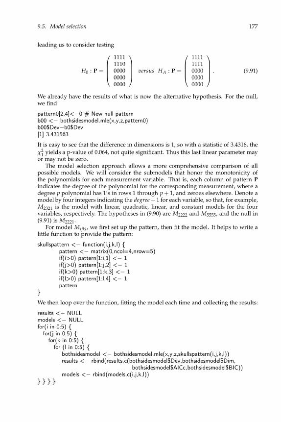
9.5. Model selection 177
leading us to consider testing
H0 : P =
11111110000000000000
versus HA : P =
11111111000000000000
. (9.91)
We already have the results of what is now the alternative hypothesis. For the null,we find
pattern0[2,4]<−0 # New null patternb00 <− bothsidesmodel.mle(x,y,z,pattern0)b00$Dev−b0$Dev[1] 3.431563
It is easy to see that the difference in dimensions is 1, so with a statistic of 3.4316, the
χ21 yields a p-value of 0.064, not quite significant. Thus this last linear parameter may
or may not be zero.The model selection approach allows a more comprehensive comparison of all
possible models. We will consider the submodels that honor the monotonicity ofthe polynomials for each measurement variable. That is, each column of pattern Pindicates the degree of the polynomial for the corresponding measurement, where adegree p polynomial has 1’s in rows 1 through p + 1, and zeroes elsewhere. Denote amodel by four integers indicating the degree+ 1 for each variable, so that, for example,M2321 is the model with linear, quadratic, linear, and constant models for the fourvariables, respectively. The hypotheses in (9.90) are M2222 and M5555, and the null in(9.91) is M2221.
For model Mijkl, we first set up the pattern, then fit the model. It helps to write alittle function to provide the pattern:
skullspattern <− function(i,j,k,l) pattern <− matrix(0,ncol=4,nrow=5)if(i>0) pattern[1:i,1] <− 1if(j>0) pattern[1:j,2] <− 1if(k>0) pattern[1:k,3] <− 1if(l>0) pattern[1:l,4] <− 1pattern
We then loop over the function, fitting the model each time and collecting the results:
results <− NULLmodels <− NULLfor(i in 0:5)
for(j in 0:5) for(k in 0:5)
for (l in 0:5) bothsidesmodel <− bothsidesmodel.mle(x,y,z,skullspattern(i,j,k,l))results <− rbind(results,c(bothsidesmodel$Dev,bothsidesmodel$Dim,
bothsidesmodel$AICc,bothsidesmodel$BIC))models <− rbind(models,c(i,j,k,l))

178 Chapter 9. Likelihood Methods
We also find the BIC-based estimates of the posterior probabilities (actually, per-centages) of the models from (9.59):
bic <− results[,4]p <− exp(−(bic−max(bic))/2) # Subtract the max to avoid underflowp <− 100∗p/sum(p)
Since each column can have from 0 to 5 ones, there are 64 = 1296 possible models. Wecould reasonably drop all the models with at least one zero in the first row withoutchanging the results. The next table has the results from fitting all 1296 models,though we just show the ten with the best (lowest) BIC’s:
Model Deviance Dimension AICc BIC PBIC
2221 2334.29 17 2369.96 2419.47 32.772222 2330.86 18 2368.62 2421.05 14.882122 2336.93 17 2372.60 2422.12 8.752321 2331.98 18 2370.01 2422.17 8.522121 2342.18 16 2375.74 2422.35 7.802322 2328.55 19 2368.69 2423.75 3.873221 2333.91 18 2371.94 2424.10 3.242231 2334.26 18 2372.29 2424.45 2.723222 2330.48 19 2370.62 2425.68 1.472223 2330.54 19 2370.68 2425.74 1.43
(9.92)
The factor multiplying the dimension dk for the AICc as in (9.88) here ranges from2.07 to 2.14, while for the BIC in (9.56), it is log(n) = log(150) = 5.01. Thus the BICwill tend to choose sparser models. The top four models for BIC are ranked numbers
3, 1, 6, and 4 for AICc. But BIC’s third best, 2122, is AICc’s 32nd best, and BIC’s fifthbest, 2121, is AICc’s 133rd best. Note that these two models are quite sparse.
Looking at the top ten models, we see they are within one or two parameters ofM2222, which is the model with linear fits for all four variables. That model is thebest under AICc, and second best under BIC. The best model under BIC shows linearfits for the first three variables, but just a constant fit for the fourth. The BIC-basedestimated probabilities for the models are quite spread out, with the top ten modelshaving a total probability of about 85%. The best model has a probability of 33%,which is high but not nearly overwhelming. All the top five have probabilities over7%.
We can also estimate the probabilities of other events. For example, the probabilitythat the maximum degree of the four polynomials is quartic sums the probabilitiesof all models for which the maximum of its indices is 5, yielding 0.73%. Similarly,the probabilities that the maximum degree is cubic, quartic, linear, and constant areestimated to be 5.03%, 30.00%, 64.23%, and 0. Thus we can be approximately 94%sure that linear or quadratics are enough. The chance any of the variables has a zeromodel (i.e., has a zero mean) is zero.
Looking at the individual variables, we can sum the probabilities of models forwhich variable i has degree j. We obtain the following, where the entries are the

9.5. Model selection 179
estimated percentages:
Maximal Basibregmatic Basialveolar NasalBreadth Height Length Height
Constant 0.05 21.53 0.00 61.70Linear 90.22 60.51 90.48 34.39Quadratic 8.89 15.64 7.50 3.23Cubic 0.78 1.96 1.80 0.61Quartic 0.07 0.35 0.23 0.08
(9.93)
Thus we can be fairly confident that linear fits are good for the first and third vari-ables, maximal breadth and basialveolar length. Basibregmatic height is also likelyto be linear, but the constant and quadratic models have nonnegligible probabilities.Nasal height is more likely to be constant than linear.
9.5.5 Example: Histamine in dogs
Now turn to the histamine in dogs example. The data are in Table 4.2, and a both-sides model is presented in (6.44). Notice that the drug effect and interaction effectare approximately opposite, which arises because the two depleted cells have approx-imately the same after values. That is, when histamine is depleted, the drug does notseem to matter. Thus we try a different model, where the contrasts are the deple-tion effect, the drug effect within the intact group, and the drug effect within thedepleted group. We also use the before measurements as covariates, and orthogonalpolynomials for the three after measurements. Thus Ya = (x, yb)βz′ + R, where
x =
1 −1 −1 01 1 0 −11 −1 1 01 1 0 1
⊗ 14 and z =
1 −1 11 0 −21 1 1
. (9.94)
Here, β is 5 × 3. We are mainly interested in the three contrasts, which are repre-sented by the middle three rows of β. The first row contains the constants, and thelast row contains the effects of the before measurements on the after measurements’coefficients. The models we will consider are then of the form Mijklm, where i, j, k, l, mare the numbers of ones in the five rows, respectively, indicating the degree + 1 of thepolynomials. If the depletion effect is in the model, then the constant effect shouldbe, and if one of the drug effects is in the model, then the depletion effect should beas well. Thus we have the constraints
0 ≤ i ≤ j ≤ k, l ≤ 3, 0 ≤ m ≤ 3. (9.95)
For example, the model with a quadratic constant, a linear depletion effect, a lineardrug effect within the intact group, a constant drug effect within the depleted group,and no before effect, has (i, j, k, l, m) = (3, 2, 2, 1, 0):
M32210 : P =
111110110100000
(9.96)
Fitting model Mijklm proceeds by first assigning the values of i, j, k, l, and m, thenusing the following:

180 Chapter 9. Likelihood Methods
x <− cbind(1,c(−1,1,−1,1),c(−1,0,1,0),c(0,−1,0,1))x <− kronecker(x,rep(1,4))xyb <− cbind(x,histamine[,1])ya <− histamine[,2:4]z <− cbind(1,c(−1,0,1),c(1,−2,1))pattern <− matrix(0,nrow=5,ncol=3)if(i>0) pattern[1,1:i] <− 1if(j>0) pattern[2,1:j] <− 1if(k>0) pattern[3,1:k] <− 1if(l>0) pattern[4,1:l] <− 1if(m>0) pattern[5,1:m] <− 1bothsidesmodel.mle(xyb,ya,z,pattern)
Here, the AICc yields sparser models, because the factor multiplying the dimen-sion dk ranges from 3.20 to 4.57 (n = 16, q = 3 and pk = 2, 3, 4, 5), while for BIC, thelog(n) = 2.77. There are 200 models this time. The top ten according to BIC are
Model Deviance Dimension AICc BIC PBIC
22200 −146.70 12 −104.03 −113.42 12.2422202 −151.70 14 −95.70 −112.89 9.3622201 −148.19 13 −96.19 −112.15 6.4832200 −147.94 13 −101.72 −111.89 5.7032202 −152.95 15 −92.95 −111.36 4.3622100 −141.28 11 −102.17 −110.78 3.2622203 −152.35 15 −92.35 −110.77 3.2422210 −146.80 13 −94.80 −110.75 3.2232201 −149.44 14 −93.44 −110.62 3.0233200 −149.40 14 −99.62 −110.58 2.96
(9.97)
The best model for both AICc and BIC is M22200, which fits a linear model to thedepletion effect, a linear model to the drug effect within the intact group, and zeroesout the drug effect within the depleted group and the before effect. As noted above,once the dogs have their histamine depleted, the drugs have no effect. Note that thetop three models are the same, except for the before effects. Since we are not reallyinterested in that effect, it is annoying that so much of the ordering of the modelsdepends on it. To clean up the presentation, we can find the marginals for the effectsof interest. That is, we sum the probabilities of all models that have a particular jkl.This leaves us with 30 probabilities, the top twelve of which are in the table below:
Model(jkl) PBIC Model(jkl) PBIC
220 45.58 222 3.08221 12.30 211 2.35210 8.76 321 1.98110 7.36 111 1.98320 7.35 310 1.43330 4.25 331 1.14
(9.98)
The top amalgamated model now has the same effects for the contrasts of interestas the previous best model, but with a fairly substantial probability of 46%. We canfurther summarize the results as in (9.93) to find the estimated percentages of the
9.6. Exercises 181
polynomial degrees for the contrasts:
Model Depletion effect Drug effect Drug effectwithin intact within depleted
Zero 0.12 0.36 75.04Constant 9.44 22.98 20.18Linear 72.78 70.92 4.56Quadratic 17.66 5.75 0.22
(9.99)
Thus the first two effects have over 99.5% probability of being nonzero, with eachover a 70% chance the effect is linear. The third effect has a 75% of being zero.
The estimated nonzero coefficients of interest for the best model in (9.97) are
Constant LinearEst. t Est. t
Depletion effect −0.259 −2.70 0.092 2.14(Depleted−Intact)Drug effect within intact 0.426 3.13 −0.140 −2.32(Trimethaphan−Morphine)
(9.100)
The average depletion effect is negative, which means the depleted dogs have lowerhistamine levels than the intact ones, which is reasonable. Also, the positive slopemeans this difference decreases over time. For the drug effect within the intact group,we see that trimethanphan is better on average, but its advantage decreases somewhatover time.
9.6 Exercises
Exercise 9.6.1. Consider the statistical model with space Y and densities f (y | θ)for θ ∈ Θ. Suppose the function g : Θ → Ω is one-to-one and onto, so that areparametrization of the model has densities f ∗(y |ω) for ω ∈ Ω, where f ∗(y |ω) =f (y | g−1(ω)). (a) Show that θ uniquely maximizes f (y | θ) over θ if and only if
ω ≡ g(θ) uniquely maximizes f ∗(y |ω) over ω. [Hint: Show that f (y | θ) > f (y | θ)for all θ′ 6= θ implies f ∗(y | ω) > f ∗(y |ω) for all ω 6= ω, and vice versa.] (b) Argue
that if θ is the MLE of θ, then g(θ) is the MLE of ω.
Exercise 9.6.2. Again consider the model with space Y and densities f (y | θ) forθ ∈ Θ, and suppose g : Θ → Ω is just onto. Let g∗ be any function of θ such thatthe joint function h(θ) = (g(θ), g∗(θ)), h : Θ → Λ, is one-to-one and onto, and set
the reparametrized density as f ∗(y |λ) = f (y | h−1(λ)). Exercise 9.6.1 shows that if
θ uniquely maximizes f (y | θ) over Θ, then λ = h(θ) uniquely maximizes f ∗(y |λ)over Λ. Argue that if θ is the MLE of θ, that it is legitimate to define g(θ) to be theMLE of ω = g(θ).
Exercise 9.6.3. Give (β, Σz) as a function of (β,γ, Σzaa·b, Σzbb) defined in (9.29) and
(9.31), and show that the latter set of parameters has space Rp×l × R(q−l)×l × Sl ×Sq−l.
Exercise 9.6.4. Verify (9.36).

182 Chapter 9. Likelihood Methods
Exercise 9.6.5. Consider the covariate example in Section 6.4.4 and (9.21), where
(Yb Ya) =
1 1 11 1 −11 −2 0
⊗ 110
µb µa
0 αa
0 βa
+ R, (9.101)
where Cov[R] = I10 ⊗ ΣR with
ΣR =
(σbb σbaσab σaa
). (9.102)
Then conditionally,
Ya | Yb = yb ∼ N
(x yb)
µ∗
αa
βa
γ
, σaa·b In
, (9.103)
where µ∗ = µa − γµb and γ = σab/σbb. (a) What is the marginal distribution of Yb?Note that its distribution depends on only (µb, σbb). Write the joint density of (Yb, Ya)as a product of the conditional and marginal densities, as in (9.35). (b) Show that theparameter vectors (µb, µa, αa, βa, ΣR) and (µ∗, αa, βa, γ, σaa·b, µb, σbb) are in one-to-onecorrespondence. (c) Show that the parameters for the conditional distribution ofYa|Yb are functionally independent of those for the marginal distribution of Yb. Thatis, the joint space of (µ∗, αa, βa, γ, σaa·b) and (µb, σbb) is a rectangle formed by theirindividual spaces. (d) Argue that therefore the MLE of (αa, βa) in the model (9.101) isthe least squares estimate from the conditional model (9.103). (Thus confirming thecorrespondence found in (9.22) and (9.23).)
Exercise 9.6.6. Consider maximizing h(Ψ) in (9.36) over Ψ ∈ Sq. (a) Let Ψ = ΓΛΓ′
be the spectral decomposition of Ψ, so that the diagonals of Λ are the eigenvaluesλ1 ≥ λ2 ≥ · · · ≥ λq ≥ 0. (Recall Theorem 1.1.) Show that
1
|Ψ|a/2e−
12 trace(Ψ
−1) =q
∏i=1
[λ−a/2i e−1/(2λi)]. (9.104)
(b) Find λi, the maximizer of λ−a/2i exp(−1/(2λi)), for each i = 1, . . . , q. (c) Show
that these λi’s satisfy the conditions on the eigenvalues of Λ. (d) Argue that then
Ψ = (1/a)Iq maximizes h(Ψ).
Exercise 9.6.7. This exercise is to show that the Wilks’ Λ test for the testing situationin Section 7.2.5 is the likelihood ratio test. We have
Y = xβ + R = (x1 x2)
(β1β2
)+ R, (9.105)
where x1 is n × p1 and x2 is n × p2. The hypotheses are
H0 : β2 = 0 versus HA : β2 6= 0. (9.106)
(a) Show that the MLE of ΣR under the alternative is ΣA = W/n, where W =Y′Q(x1,x2)Y. (b) Show that Σ0 = (W + B)/n, where W + B = Y′Qx1 Y. (c) Find
the κ so that likelihood ratio statistic LR in (9.41) equals Λκ for Λ = |W|/|B + W|.This Λ is Wilks’ Λ as in (7.35).

9.6. Exercises 183
Exercise 9.6.8. Now consider the model with partitioning
Y = (Y1 Y2) = (x1 x2)
(β11 β21β12 β22
)+ R, (9.107)
where Y1 is n × l∗, Y2 is n × (q − l∗), β11 is p1 × l∗, x1 is n × p1, and x2 is n × p2. Wetest
H0 : β11 = 0 versus HA : β11 6= 0. (9.108)
(a) Find the conditional distribution of Y2|Y1 = y1 and the marginal distributionof Y1. (b) Argue that that conditional distribution is the same under the null andalternative hypotheses, hence we can find the likelihood ratio test by using just themarginal distribution of Y1. (c) Use Exercise 9.6.7 to show that the likelihood ratiotest is equivalent to Wilks’ Λ test. What are the parameters for the Λ in this case?
Exercise 9.6.9. Argue that the likelihood ratio test of (9.46) based on (9.45) is equiva-lent to Wilks’ Λ test, and specify the parameters for the Λ. [Hint: Use Exercise 9.6.8to show that the test can be based on the conditional distribution in (9.47), then makethe appropriate identifications of parameters.]
Exercise 9.6.10. Consider the multivariate regression model (4.9), where ΣR is known.(a) Use (9.80) to show that
l(β ; y)− l(β ; y) = − 1
2trace(Σ−1
R (β− β)′x′x(β − β)). (9.109)
(b) Show that in this case, (9.66) is actually an equality, and give H, which is a functionof ΣR and x′x.
Exercise 9.6.11. (a) Show that for the ΣR in (9.81),
E[Σ−1R ] =
n
n − p − q − 1Σ−1R . (9.110)
(b) Show that
U ∼ N(0, (In + Px)⊗ ΣR) (9.111)
for U in (9.83), and thus
E[U′U] = (n + p)ΣR. (9.112)
(c) Show that
trace(E[Σ−1R ]E[U′U]) = nq
n + p
n − p − q − 1. (9.113)
(d) Finally, show that
trace(E[Σ−1R ]E[U′U])− nq = 2
n
n − p − q − 1
(pq +
q(q + 1)
2
), (9.114)
proving (9.85).
Exercise 9.6.12. Show that in (9.85), ∆ → 2dM as n → ∞.

184 Chapter 9. Likelihood Methods
Exercise 9.6.13. Show that in (9.59), if we take the prior probabilities as
πk ∝
(√n
e
)dk
, (9.115)
where dk is the dimension of Model k, then the model that maximizes the estimatedposterior probability is the model with the lowest AIC. Note that except for verysmall n, this prior places relatively more weight on higher-dimensional models.
Exercise 9.6.14 (Prostaglandin). Continue with the prostaglandin data from Exercise7.6.16. (a) Find the maximum likelihood estimates and standard errors for the coef-ficients in the model with just one cycle. Compare these results to the least squaresestimates and standard errors. Which method produces the larger standard errors?Approximately how much larger are they? (b) Find the BIC’s and the correspondingestimated probabilities for the following models: constant, one cycle, one and twocycle, all cycles. Which has the best BIC? Does it have a relatively high estimatedprobability?
Exercise 9.6.15 (Caffeine). This question continues with the caffeine data in Exercises4.4.4 and 6.6.11. Start with the both-sides model Y = xβz′ + R, where as beforethe Y is 2 × 28, the first column being the scores without caffeine, and the secondbeing the scores with caffeine. The x is a 28 × 3 matrix for the three grades, withorthogonal polynomials. The linear vector is (−1′9, 0′10, 1′9)
′ and the quadratic vectoris (1′9,−1.81′10, 1′9)
′. The z looks at the sum and difference of scores:
z =
(1 −11 1
). (9.116)
The goal of this problem is to use BIC to find a good model, choosing among the con-stant, linear and quadratic models for x, and the “overall mean” and “overall mean+ difference models” for the scores. (a) For each of the 6 models, find the deviance,number of free parameters, BIC, and estimated probability. (b) Which model hashighest probability? (c) What is the chance that the difference effect is in the model?(d) Find the MLE of β for the best model.
Exercise 9.6.16 (Leprosy). Continue with the leprosy example from Exercise 9.6.5. Weare interested in finding a good model, but are not interested in the parameters µb orσbb. Thus we can base the analysis solely on the conditional model in (9.103). (a) Find
the BIC’s and corresponding probability estimates for the 23 = 8 models found bysetting subsets of (αa, βa, γ) to 0. Which model has the best BIC? What is its estimatedprobability? (b) What is the probability (in percent) that the drug vs. placebo effectis in the model? The Drug A vs. Drug D effect? The before effect (i.e.,γ 6= 0)?
Exercise 9.6.17 (Mouth sizes). Section 7.5.1 presents Mallows’ Cp for a number ofmodels fit to the mouth size data. Fit the same models, but find their BIC’s. (a) Whichmodel has the best BIC? Which has the second best? What is the total estimatedprobability of those two models? Are they the same as the best two models chosenby Cp in (7.83)? (b) What is the estimated probability that the two curves are different,i.e., that the δj’s are not all zero? (c) Find the estimated probabilities for each degree ofpolynomial (zero, constant, linear, quadratic, cubic) for each effect (boys, girls−boys),analogous to the table in (9.99).

9.6. Exercises 185
Exercise 9.6.18. (This is a discussion question, in that there is no exact answer. Yourreasoning should be sound, though.) Suppose you are comparing a number of mod-els using BIC, and the lowest BIC is bmin. How much larger than bmin would a BIChave to be for you to consider the corresponding model ignorable? That is, what is δso that models with BIC > bmin + δ don’t seem especially viable. Why?
Exercise 9.6.19. Often, in hypothesis testing, people misinterpret the p-value to be theprobability that the null is true, given the data. We can approximately compare thetwo values using the ideas in this chapter. Consider two models, the null (M0) andalternative (MA), where the null is contained in the alternative. Let deviance0 anddevianceA be their deviances, and dim0 and dimA be their dimensions, respectively.Supposing that the assumptions are reasonable, the p-value for testing the null is
p-value = P[χ2ν > δ], where ν = dimA −dim0 and δ = deviance0 −devianceA. (a)
Give the BIC-based estimate of the probability of the null for a given ν, δ and samplesize n. (b) For each of various values of n and ν (e.g, n = 1, 5, 10, 25, 100, 1000 andν = 1, 5, 10, 25), find the δ that gives a p-value of 5%, and find the correspondingestimate of the probability of the null. (c) Are the probabilities of the null close to5%? What do you conclude?


Chapter 10
Models on Covariance Matrices
The models so far have been on the means of the variables. In this chapter, we lookat some models for the covariance matrix. We start with testing the equality of twoor more covariance matrices, then move on to testing independence and conditionalindependence of sets of variables. Next is factor analysis, where the relationshipsamong the variables are assumed to be determined by latent (unobserved) variables.Principal component analysis is sometimes thought of as a type of factor analysis,although it is more of a decomposition than actual factor analysis. See Section 13.1.5.We conclude with a particular class of structural models, called invariant normal mod-els.
We will base our hypothesis tests on Wishart matrices (one, or several independentones). In practice, these matrices will often arise from the residuals in linear models,especially the Y′QxY as in (6.14). If U ∼ Wishartq(ν, Σ), where Σ is invertible andν ≥ q, then the likelihood is
L(Σ; U) = |Σ|−ν/2 e−12 trace(Σ
−1U). (10.1)
The likelihood follows from the density in (8.70). An alternative derivation is to notethat by (8.53), Z ∼ N(0, Iν ⊗ Σ) has likelihood L∗(Σ; z) = L(Σ; z′z). Thus z′z is asufficient statistic, and it can be shown that the likelihood for any X is the same as
the likelihood for its sufficient statistic. Since Z′Z =D U, (10.1) is the likelihood forU.
Recall from (5.51) that S+q denotes the set of q × q positive definite symmetric
matrices. Then Lemma 9.1 shows that the MLE of Σ ∈ S+q based on (10.1) is
Σ =U
ν, (10.2)
and the maximum likelihood is
L(Σ ; U) =
∣∣∣∣U
ν
∣∣∣∣−ν/2
e−12 νq. (10.3)
187

188 Chapter 10. Covariance Models
10.1 Testing equality of covariance matrices
We first suppose we have two groups, e.g., boys and girls, and wish to test whethertheir covariance matrices are equal. Let U1 and U2 be independent, with
Ui ∼ Wishartq(νi, Σi), i = 1, 2. (10.4)
The hypotheses are then
H0 : Σ1 = Σ2 versus HA : Σ1 6= Σ2, (10.5)
where both Σ1 and Σ2 are in S+q . (That is, we are not assuming any particular struc-
ture for the covariance matrices.) We need the likelihoods under the two hypotheses.Because the Ui’s are independent,
L(Σ1, Σ2; U1, U2) = |Σ1|−ν1/2 e−12 trace(Σ
−11 U1)|Σ2|−ν2/2 e−
12 trace(Σ
−12 U2), (10.6)
which, under the null hypothesis, becomes
L(Σ, Σ; U1, U2) = |Σ|−(ν1+ν2)/2 e−12 trace(Σ
−1(U1+U2)), (10.7)
where Σ is the common value of Σ1 and Σ2. The MLE under the alternative hypoth-esis is found by maximizing (10.5), which results in two separate maximizations:
Under HA: ΣA1 =U1
ν1, ΣA2 =
U2
ν2. (10.8)
Under the null, there is just one Wishart, U1 + U2, so that
Under H0: Σ01 = Σ02 =U1 + U2
ν1 + ν2. (10.9)
Thus
supHA
L =
∣∣∣∣U1
ν1
∣∣∣∣−ν1/2
e−12 ν1q
∣∣∣∣U2
ν2
∣∣∣∣−ν2/2
e−12 ν2q, (10.10)
and
supH0
L =
∣∣∣∣U1 + U2
ν1 + ν2
∣∣∣∣−(ν1+ν2)/2
e−12 (ν1+ν2)q. (10.11)
Taking the ratio, note that the parts in the e cancel, hence
LR =supHA
L
supH0L
=|U1/ν1|−ν1/2 |U2/ν2|−ν2/2
|(U1 + U2)/(ν1 + ν2)|−(ν1+ν2)/2. (10.12)
And
2 log(LR) = (ν1 + ν2) log
∣∣∣∣U1 + U2
ν1 + ν2
∣∣∣∣− ν1 log
∣∣∣∣U1
ν1
∣∣∣∣− ν2 log
∣∣∣∣U2
ν2
∣∣∣∣ . (10.13)
Under the null hypothesis, 2 log(LR) approaches a χ2 as in (9.41). To figure outthe degrees of freedom, we have to find the number of free parameters under each

10.1. Testing equality 189
hypothesis. A Σ ∈ S+q , unrestricted, has q(q + 1)/2 free parameters, because of the
symmetry. Under the alternative, there are two such sets of parameters. Thus,
dim(H0) = q(q + 1)/2, dim(HA) = q(q + 1)
⇒ dim(HA)− dim(H0) = q(q + 1)/2. (10.14)
Thus, under H0,
2 log(LR) −→ χ2q(q+1)/2. (10.15)
10.1.1 Example: Grades data
Using the grades data on n = 107 students in (4.11), we compare the covariancematrices of the men and women. There are 37 men and 70 women, so that the samplecovariance matrices have degrees of freedom ν1 = 37 − 1 = 36 and ν2 = 70 − 1 = 69,respectively. Their estimates are:
Men:1
ν1U1 =
166.33 205.41 106.24 51.69 62.20205.41 325.43 206.71 61.65 69.35106.24 206.71 816.44 41.33 41.8551.69 61.65 41.33 80.37 50.3162.20 69.35 41.85 50.31 97.08
, (10.16)
and
Women:1
ν2U2 =
121.76 113.31 58.33 40.79 40.91113.31 212.33 124.65 52.51 50.6058.33 124.65 373.84 56.29 74.4940.79 52.51 56.29 88.47 60.9340.91 50.60 74.49 60.93 112.88
. (10.17)
These covariance matrices are clearly not equal, but are the differences significant?The pooled estimate, i.e., the common estimate under H0, is
1
ν1 + ν2(U1 + U2) =
137.04 144.89 74.75 44.53 48.21144.89 251.11 152.79 55.64 57.0374.75 152.79 525.59 51.16 63.3044.53 55.64 51.16 85.69 57.2948.21 57.03 63.30 57.29 107.46
. (10.18)
Then
2 log(LR) = (ν1 + ν2) log
∣∣∣∣U1 + U2
ν1 + ν2
∣∣∣∣− ν1 log
∣∣∣∣U1
ν1
∣∣∣∣− ν2 log
∣∣∣∣U2
ν2
∣∣∣∣
= 105 log(2.6090 × 10¹⁰)− 36 log(2.9819 × 10¹⁰)− 69 log(1.8149 × 10¹⁰)
= 20.2331. (10.19)
The degrees of freedom for the χ2 is q(q + 1)/2 = 5 × 6/2 = 15. The p-value is 0.16,which shows that we have not found a significant difference between the covariancematrices.

190 Chapter 10. Covariance Models
10.1.2 Testing the equality of several covariance matrices
It is not hard to extend the test to testing the equality of more than two covariancematrices. That is, we have U1, . . . , Um, independent, Ui ∼ Wishartl(νi, Σi), and wishto test
H0 : Σ1 = · · · = Σm versus HA : not. (10.20)
Then
2 log(LR) = (ν1 + · · ·+νm) log
∣∣∣∣U1 + · · ·+ Um
ν1 + · · ·+ νm
∣∣∣∣− ν1 log
∣∣∣∣U1
ν1
∣∣∣∣− · · · − νm log
∣∣∣∣Um
νm
∣∣∣∣ ,
(10.21)
and under the null,
2 log(LR) −→ χ2d f , d f = (m − 1)q(q + 1)/2. (10.22)
This procedure is Bartlett’s test for the equality of covariances.
10.2 Testing independence of two blocks of variables
In this section, we assume U ∼ Wishartq(ν, Σ), and partition the matrices:
U =
(U11 U12U21 U22
)and Σ =
(Σ11 Σ12Σ21 Σ22
), (10.23)
where
U11 and Σ11 are q1 × q1, and U22 and Σ22 are q2 × q2; q = q1 + q2. (10.24)
Presuming the Wishart arises from multivariate normals, we wish to test whether thetwo blocks of variables are independent, which translates to testing
H0 : Σ12 = 0 versus HA : Σ12 6= 0. (10.25)
Under the alternative, the likelihood is just the one in (10.1), hence
supHA
L(Σ; U) =
∣∣∣∣U
ν
∣∣∣∣−ν/2
e−12 νq. (10.26)
Under the null, because Σ is then block diagonal,
|Σ| = |Σ11| |Σ22| and trace(Σ−1U) = trace(Σ−111 U11) + trace(Σ−1
22 U22). (10.27)
Thus the likelihood under the null can be written
|Σ11|−ν/2 e−12 trace(Σ
−111 U11) × |Σ22|−ν/2 e−
12 trace(Σ
−122 U22). (10.28)
The two factors can be maximized separately, so that
supH0
L(Σ; U) =
∣∣∣∣U11
ν
∣∣∣∣−ν/2
e−12 νq1 ×
∣∣∣∣U22
ν
∣∣∣∣−ν/2
e−12 νq2 . (10.29)

10.2. Testing independence 191
Taking the ratio of (10.26) and (10.28), the parts in the exponent of the e againcancel, hence
2 log(LR) = ν (log(|U11/ν|) + log(|U22/ν|)− log(|U/ν|)). (10.30)
(The ν’s in the denominators of the determinants cancel, so they can be erased ifdesired.)
Section 13.3 considers canonical correlations, which are a way to summarize rela-tionships between two sets of variables.
10.2.1 Example: Grades data
Continuing Example 10.1.1, we start with the pooled covariance matrix Σ = (U1 +U2)/(ν1 + ν2), which has q = 5 and ν = 105. Here we test whether the first threevariables (homework, labs, inclass) are independent of the last two (midterms, final),so that q1 = 3 and q2 = 2. Obviously, they should not be independent, but we willtest it formally. Now
2 log(LR) = ν (log(|U11/ν|) + log(|U22/ν|)− log(|U/ν|))= 28.2299. (10.31)
Here the degrees of freedom in the χ2 are q1 × q2 = 6, because that is the number ofcovariances we are setting to 0 in the null. Or you can count
dim(HA) = q(q + 1)/2 = 15,
dim(H0) = q1(q1 + 1)/2 + q2(q2 + 1)/2 = 6 + 3 = 9, (10.32)
which has dim(HA)−dim(H0) = 6. In either case, the result is clearly significant (thep-value is less than 0.0001), hence indeed the two sets of scores are not independent.
Testing the independence of several block of variables is almost as easy. Considerthe three variables homework, inclass, and midterms, which have covariance
Σ =
σ11 σ13 σ14σ31 σ33 σ34σ41 σ43 σ44
. (10.33)
We wish to test whether the three are mutually independent, so that
H0 : σ13 = σ14 = σ34 = 0 versus HA : not. (10.34)
Under the alternative, the estimate of Σ is just the usual one from (10.18), wherewe pick out the first, third, and fourth variables. Under the null, we have three
independent variables, so σii = Uii/ν is just the appropriate diagonal from Σ. Thenthe test statistic is
2 log(LR) = ν (log(|U11/ν|) + log(|U33/ν|) + log(|U44/ν|)− log(|U∗/ν|))= 30.116, (10.35)
where U∗ contains just the variances and covariances of the variables 1, 3, and 4. Wedo not need the determinant notation for the Uii, but leave it in for cases in whichthe three blocks of variables are not 1 × 1. The degrees of freedom for the χ2 is then3, because we are setting three free parameters to 0 in the null. Clearly that is asignificant result, i.e., these three variables are not mutually independent.

192 Chapter 10. Covariance Models
10.2.2 Example: Testing conditional independence
Imagine that we have (at least) three blocks of variables, and wish to see whetherthe first two are conditionally independent given the third. The process is exactlythe same as for testing independence, except that we use the conditional covariancematrix. That is, suppose
Y = (Y1, Y2, Y3) ∼ N(xβz′, In ⊗ ΣR), Yi is n × qi, q = q1 + q2 + q3, (10.36)
where
ΣR =
Σ11 Σ12 Σ13Σ21 Σ22 Σ23
Σ31 Σ32 Σ33
, (10.37)
so that Σii is qi × qi. The null hypothesis is
H0 : Y1 and Y2 are conditionally independent given Y3. (10.38)
The conditional covariance matrix is
Cov[(Y1, Y2) |Y3 = y3] =
(Σ11 Σ12Σ21 Σ22
)−(
Σ13Σ23
)Σ−133
(Σ31 Σ32
)
=
(Σ11 − Σ13Σ
−133 Σ31 Σ12 − Σ13Σ
−133 Σ32
Σ21 − Σ23Σ−133 Σ31 Σ22 − Σ23Σ
−133 Σ32
)
≡(
Σ11·3 Σ12·3Σ21·3 Σ22·3
). (10.39)
Then the hypotheses are
H0 : Σ12·3 = 0 versus HA : Σ12·3 6= 0. (10.40)
Letting U/ν be the usual estimator of ΣR, where
U = Y′QxY ∼ Wishart(q1+q2+q3)(ν, ΣR), ν = n − p, (10.41)
we know from Proposition 8.1 that the conditional covariance is also Wishart, butloses q3 degrees of freedom:
U(1:2)(1:2)·3 ≡(
U11·3 U12·3U21·3 U22·3
)
∼ Wishart(q1+q2)
(ν − q3,
(Σ11·3 Σ12·3Σ21·3 Σ22·3
)). (10.42)
(The U is partitioned analogously to the ΣR.) Then testing the hypothesis Σ12·3 hereis the same as (10.30) but after dotting out 3:
2 log(LR) = (ν − q3) ( log(|U11·3/(ν − q3)|) + log(|U22·3/(ν − q3)|)− log(|U(1:2)(1:2)·3/(ν − q3)|)), (10.43)
which is asymptotically χ2q1q2
under the null.

10.2. Testing independence 193
An alternative (but equivalent) method for calculating the conditional covarianceis to move the conditioning variables Y3 to the x matrix, as we did for covariates.Thus, leaving out the z,
(Y1 Y2) | Y3 = y3 ∼ N(x∗β∗, In ⊗ Σ∗), (10.44)
where
x∗ = (x y3) and Σ∗ =
(Σ11·3 Σ12·3Σ21·3 Σ22·3
). (10.45)
Then
U(1:2)(1:2)·3 = (Y1 Y2)′Qx∗(Y1 Y2). (10.46)
See Exercise 10.5.5.We note that there appears to be an ambiguity in the denominators of the Ui’s for
the 2 log(LR). That is, if we base the likelihood on the original Y of (10.36), then thedenominators will be n. If we use the original U in (10.41), the denominators willbe n − p. And what we actually used, based on the conditional covariance matrixin (10.42), was n − p − q3. All three possibilities are fine in that the asymptotics asn → ∞ are valid. We chose the one we did because it is the most focussed, i.e., thereare no parameters involved (e.g., β) that are not directly related to the hypotheses.
Testing the conditional independence of three or more blocks of variables, givenanother block, again uses the dotted-out Wishart matrix. For example, consider Ex-ample 10.2.1 with variables homework, inclass, and midterms, but test whether thosethree are conditionally independent given the “block 4” variables, labs and final. Theconditional U matrix is now denoted U(1:3)(1:3)·4, and the degrees of freedom are
ν − q4 = 105 − 2 = 103, so that the estimate of the conditional covariance matrix is
σ11·4 σ12·4 σ13·4σ21·4 σ22·4 σ23·4σ31·4 σ32·4 σ33·4
=
1
ν − q4U(1:3)(1:3)·4
=
51.9536 −18.3868 5.2905−18.3868 432.1977 3.8627
5.2905 3.8627 53.2762
. (10.47)
Then, to test
H0 : σ12·4 = σ13·4 = σ23·4 = 0 versus HA : not, (10.48)
we use the statistic analogous to (10.35),
2 log(LR) = (ν − q4) (log(|U11·4/(ν − q4)|) + log(|U22·4/(ν − q4)|)+ log(|U33·4/(ν − q4)|)− log(|U(1:3)(1:3)·4/(ν − q4)|))
= 2.76. (10.49)
The degrees of freedom for the χ2 is again 3, so we accept the null: There does notappear to be a significant relationship among these three variables given the labs andfinal scores. This implies, among other things, that once we know someone’s labs andfinal scores, knowing the homework or inclass will not help in guessing the midtermsscore. We could also look at the sample correlations, unconditionally (from (10.18))

194 Chapter 10. Covariance Models
and conditionally:
UnconditionalHW InClass Midterms
HW 1.00 0.28 0.41InClass 0.28 1.00 0.24Midterms 0.41 0.24 1.00
Conditional on Labs, FinalHW InClass Midterms1.00 −0.12 0.10
−0.12 1.00 0.030.10 0.03 1.00
(10.50)Notice that the conditional correlations are much smaller than the unconditional
ones, and the conditional correlation between homework and inclass scores is nega-tive, though not significantly so. Thus it appears that the labs and final scores explainthe relationships among the other variables.
Remark
Graphical models are important and useful models for studying more complicatedindependence and conditional independence relations among variables. Some refer-ences: Whitaker [1990], Jordan [1999], and Koller and Friedman [2009].
10.3 Factor analysis
The example above suggested that the relationship among three variables could beexplained by two other variables. The idea behind factor analysis is that the relation-ships (correlations, to be precise) of a set of variables can be explained by a numberof other variables, called factors. The kicker here is that the factors are not observed.Spearman [1904] introduced the idea based on the notion of a “general intelligence”factor. This section gives the very basics of factor analysis. More details can be foundin Lawley and Maxwell [1971], Harman [1976] and Basilevsky [1994], as well as manyother books.
The model we consider sets Y to be the n × q matrix of observed variables, and Xto be the n × p matrix of factor variables, which we do not observe. Assume
(X Y
)∼ N(D
(δ γ
), In ⊗ Σ), Σ =
(ΣXX ΣXYΣYX ΣYY
), (10.51)
where D is an n × k design matrix (e.g., to distinguish men from women), and δ
(k × p) and γ (k × q) are the parameters for the means of X and Y, respectively. Factoranalysis is not primarily concerned with the means (that is what the linear modelsare for), but with the covariances. The key assumption is that the variables in Yare conditionally independent given X, which means the conditional covariance isdiagonal:
Cov[Y | X = x] = In ⊗ ΣYY·X = In ⊗ Ψ = In ⊗
ψ11 0 · · · 00 ψ22 · · · 0...
.... . .
...0 0 · · · ψqq
. (10.52)
Writing out the conditional covariance matrix, we have
Ψ = ΣYY − ΣYXΣ−1XXΣXY ⇒ ΣYY = ΣYXΣ
−1XXΣXY + Ψ, (10.53)
10.3. Factor analysis 195
so that marginally,
Y ∼ N(Dγ, In ⊗ (ΣYXΣ−1XXΣXY + Ψ)). (10.54)
Because Y is all we observe, we cannot estimate ΣXY or ΣXX separately, but only the
function ΣYXΣ−1XXΣXY. Note that if we replace X with X∗ = XA for some invertible
matrix A,ΣYXΣ
−1XXΣXY = ΣYX∗Σ
−1X∗X∗ΣX∗Y, (10.55)
so that the distribution of Y is unchanged. See Exercise 10.5.6. Thus in order toestimate the parameters, we have to make some restrictions. Commonly it is assumedthat ΣXX = Ip, and the mean is zero:
X ∼ N(0, In ⊗ Ip). (10.56)
Then, letting β = Σ−1XXΣXY = ΣXY,
Y ∼ N(Dγ, In ⊗ (β′β + Ψ)). (10.57)
Or, we can write the model as
Y = Dγ + Xβ+ R, X ∼ N(0, In ⊗ Ip), R ∼ N(0, In ⊗ Ψ), (10.58)
where X and R are independent. The equation decomposes each variable (column)in Y into the fixed mean plus the part depending on the factors plus the parts uniqueto the individual variables. The element βij is called the loading of factor i on thevariable j. The variance ψj is the unique variance of variable j, i.e., the part notexplained by the factors. Any measurement error is assumed to be part of the uniquevariance.
There is the statistical problem of estimating the model, meaning the β′β and Ψ
(and γ, but we already know about that), and the interpretative problem of findingand defining the resulting factors. We will take these concerns up in the next twosubsections.
10.3.1 Estimation
We estimate the γ using least squares as usual, i.e.,
γ = (D′D)−1D′Y. (10.59)
Then the residual sum of squares matrix is used to estimate the β and Ψ:
U = Y′QDY ∼ Wishartq(ν,β′β+ Ψ), ν = n − k. (10.60)
The parameters are still not estimable, because for any p × p orthogonal matrixΓ, (Γβ)′(Γβ) yields the same β′β. We can use the QR decomposition from Theorem5.4. Our β is p × q with p < q. Write β = (β1,β2), where β1 has the first p columnsof β. We apply the QR decomposition to β1, assuming the columns are linearlyindependent. Then β1 = QT, where Q is orthogonal and T is upper triangular withpositive diagonal elements. Thus we can write Q′β1 = T, or
Q′β = Q′ ( β1 β2)=(
T T∗ ) ≡ β∗, (10.61)
196 Chapter 10. Covariance Models
where T∗ is some p × (q − p) matrix. E.g., with p = 3, q = 5,
β∗ =
β∗11 β∗12 β∗13 β∗14 β∗150 β∗22 β∗23 β∗24 β∗250 0 β∗33 β∗34 β∗35
, (10.62)
where the β∗ii’s are positive. If we require that β satisfies constraints (10.62), then itis estimable. (Exercise 10.5.7.) Note that there are p(p − 1)/2 non-free parameters(since βij = 0 for i > j), which means the number of free parameters in the model
is pq − p(p − 1)/2 for the β part, and q for Ψ. Thus for the p-factor model Mp, thenumber of free parameters is
dp ≡ dim(Mp) = q(p + 1)− p(p − 1)
2. (10.63)
(We are ignoring the parameters in the γ, because they are the same for all the modelswe consider.) In order to have a hope of estimating the factors, the dimension of thefactor model cannot exceed the dimension of the most general model, ΣYY ∈ S+
q ,
which has q(q + 1)/2 parameters. Thus for identifiability we need
q(q + 1)
2− dp =
(q − p)2 − p − q
2≥ 0. (10.64)
E.g., if there are q = 10 variables, at most p = 6 factors can be estimated.There are many methods for estimating β and Ψ. As in (10.1), the maximum
likelihood estimator maximizes
L(β, Ψ; U) =1
|β′β + Ψ|ν/2e−
12 trace((β′β+Ψ)−1U) (10.65)
over β satisfying (10.62) and Ψ being diagonal. There is not a closed form solution tothe maximization, so it must be done numerically. There may be problems, too, such
as having one or more of the ψj’s being driven to 0. It is not obvious, but if β and Ψ
are the MLE’s, then the maximum of the likelihood is, similar to (10.3),
L(β, Ψ; U) =1
|β′β+ Ψ|ν/2e−
12 νq. (10.66)
See Section 9.4 of Mardia, Kent, and Bibby [1979].Typically one is interested in finding the simplest model that fits. To test whether
the p-factor model fits, we use the hypotheses
H0 : ΣYY = β′β + Ψ, β is p × q versus HA : ΣYY ∈ S+q . (10.67)
The MLE for HA is ΣYY = U/ν, so that
LR =
(|β′β + Ψ||U/ν|
)ν/2
. (10.68)
Now
2 log(LR) = ν(log(|β′β+ Ψ|)− log(|U/ν|)), (10.69)

10.3. Factor analysis 197
which is asymptotically χ2d f with d f being the difference in (10.64). Bartlett suggests
a slight adjustment to the factor ν, similar to the Box approximation for Wilks’ Λ, sothat under the null,
2 log(LR)∗ = (ν − 2q + 5
6− 2p
3)(log(|β′β+ Ψ|)− log(|U/ν|)) −→ χ2
d f , (10.70)
where from (10.64),
d f =(q − p)2 − p − q
2. (10.71)
Alternatively, one can use AIC (9.56) or BIC (9.57) to assess Mp for several p.Because νq is the same for all models, we can take
deviance(Mp(β, Ψ) ; y) = ν log(|β′β+ Ψ|), (10.72)
so that
BIC(Mp) = ν log(|β′β + Ψ|) + log(ν) (q(p + 1)− p(p − 1)/2) , (10.73)
AIC(Mp) = ν log(|β′β + Ψ|) + 2 (q(p + 1)− p(p − 1)/2) . (10.74)
10.3.2 Describing the factors
Once you have decided on the number p of factors in the model and the estimate β,
you have a choice of rotations. That is, since Γβ for any p × p orthogonal matrix Γ
has exactly the same fit, you need to choose the Γ. There are a number of criteria. The
varimax criterion tries to pick a rotation so that the loadings (βij’s) are either large inmagnitude, or close to 0. The hope is that it is then easy to interpret the factors byseeing which variables they load heavily upon. Formally, the varimax rotation is thatwhich maximizes the sum of the variances of the squares of the elements in each row.
That is, if F is the p × q matrix consisting of the squares of the elements in Γβ, thenthe varimax rotation is the Γ that maximizes trace(FHqF′), Hq being the centeringmatrix (1.12). There is nothing preventing you from trying as many Γ’s as you wish.It is an art to find a rotation and interpretation of the factors.
The matrix X, which has the scores of the factors for the individuals, is unobserved,but can be estimated. The joint distribution is, from (10.51) with the assumptions(10.56),
(X Y
)∼ N
((0 Dγ
), In ⊗ Σ
), Σ =
(Ip β
β′ β′β + Ψ
). (10.75)
Then given the observed Y:
X | Y = y ∼ N(α∗ + yβ∗, In ⊗ ΣXX·Y), (10.76)
whereβ∗ = (β′β+ Ψ)−1β′, α∗ = −Dγβ∗, (10.77)
and
ΣXX·Y = Ip − β(β′β+ Ψ)−1β′. (10.78)
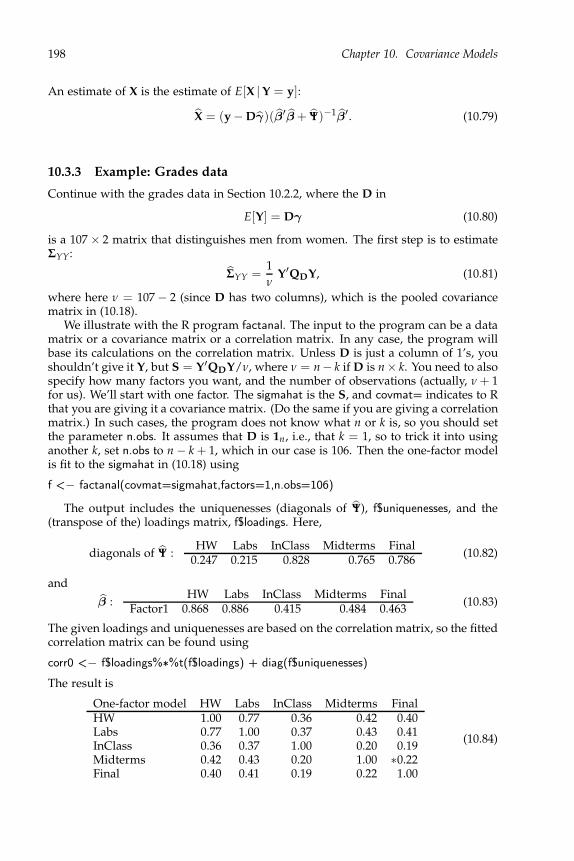
198 Chapter 10. Covariance Models
An estimate of X is the estimate of E[X | Y = y]:
X = (y − Dγ)(β′β+ Ψ)−1β′. (10.79)
10.3.3 Example: Grades data
Continue with the grades data in Section 10.2.2, where the D in
E[Y] = Dγ (10.80)
is a 107 × 2 matrix that distinguishes men from women. The first step is to estimateΣYY:
ΣYY =1
νY′QDY, (10.81)
where here ν = 107 − 2 (since D has two columns), which is the pooled covariancematrix in (10.18).
We illustrate with the R program factanal. The input to the program can be a datamatrix or a covariance matrix or a correlation matrix. In any case, the program willbase its calculations on the correlation matrix. Unless D is just a column of 1’s, youshouldn’t give it Y, but S = Y′QDY/ν, where ν = n − k if D is n × k. You need to alsospecify how many factors you want, and the number of observations (actually, ν + 1for us). We’ll start with one factor. The sigmahat is the S, and covmat= indicates to Rthat you are giving it a covariance matrix. (Do the same if you are giving a correlationmatrix.) In such cases, the program does not know what n or k is, so you should setthe parameter n.obs. It assumes that D is 1n, i.e., that k = 1, so to trick it into usinganother k, set n.obs to n − k + 1, which in our case is 106. Then the one-factor modelis fit to the sigmahat in (10.18) using
f <− factanal(covmat=sigmahat,factors=1,n.obs=106)
The output includes the uniquenesses (diagonals of Ψ), f$uniquenesses, and the(transpose of the) loadings matrix, f$loadings. Here,
diagonals of Ψ :HW Labs InClass Midterms Final
0.247 0.215 0.828 0.765 0.786(10.82)
and
β :HW Labs InClass Midterms Final
Factor1 0.868 0.886 0.415 0.484 0.463(10.83)
The given loadings and uniquenesses are based on the correlation matrix, so the fittedcorrelation matrix can be found using
corr0 <− f$loadings%∗%t(f$loadings) + diag(f$uniquenesses)
The result is
One-factor model HW Labs InClass Midterms FinalHW 1.00 0.77 0.36 0.42 0.40Labs 0.77 1.00 0.37 0.43 0.41InClass 0.36 0.37 1.00 0.20 0.19Midterms 0.42 0.43 0.20 1.00 ∗0.22Final 0.40 0.41 0.19 0.22 1.00
(10.84)

10.3. Factor analysis 199
Compare that to the observed correlation matrix, which is in the matrix f$corr:
Unrestricted model HW Labs InClass Midterms FinalHW 1.00 0.78 0.28 0.41 0.40Labs 0.78 1.00 0.42 0.38 0.35InClass 0.28 0.42 1.00 0.24 0.27Midterms 0.41 0.38 0.24 1.00 ∗0.60Final 0.40 0.35 0.27 0.60 1.00
(10.85)
The fitted correlations are reasonably close to the observed ones, except for themidterms/final correlation: The actual is 0.60, but the estimate from the one-factormodel is only 0.22. It appears that this single factor is more focused on other correla-tions.
For a formal goodness-of-fit test, we have
H0 : One-factor model versus HA : Unrestricted. (10.86)
We can use either the correlation or covariance matrices, as long as we are consistent,and since factanal gives the correlation, we might as well use that. The MLE underHA is then corrA, the correlation matrix obtained from S, and under H0 is corr0. Then
2 log(LR) = ν(log(|β′β + Ψ|)− log(|S|)) (10.87)
is found in R using
105∗log(det(corr0)/det(f$corr))
yielding the value 37.65. It is probably better to use Bartlett’s refinement (10.70),
(105 − (2∗5+5)/6−2/3)∗log(det(corr0)/det(f$corr))
which gives 36.51. This value can be found in f$STATISTIC, or by printing out f. The
degrees of freedom for the statistic in (10.71) is ((q − p)2 − p − q)/2 = 5, since p = 1and q = 5. Thus H0 is rejected: The one-factor model does not fit.
Two factors
With small q, we have to be careful not to ask for too many factors. By (10.64), two isthe maximum when q = 5. In R, we just need to set factors=2 in the factanal function.
The χ2 for goodness-of-fit is 2.11, on one degree of freedom, hence the two-factormodel fits fine. The estimated correlation matrix is now
Two-factor model HW Labs InClass Midterms FinalHW 1.00 0.78 0.35 0.40 0.40Labs 0.78 1.00 0.42 0.38 0.35InClass 0.35 0.42 1.00 0.24 0.25Midterms 0.40 0.38 0.24 1.00 0.60Final 0.40 0.35 0.25 0.60 1.00
(10.88)
which is quite close to the observed correlation matrix (10.85) above. Only the In-Class/HW correlation is a bit off, but not by much.

200 Chapter 10. Covariance Models
The uniquenesses and loadings for this model are
diagonals of Ψ :HW Labs InClass Midterms Final0.36 0.01 0.80 0.48 0.30
(10.89)
and
β :HW Labs InClass Midterms Final
Factor 1 0.742 0.982 0.391 0.268 0.211Factor 2 0.299 0.173 0.208 0.672 0.807
(10.90)
The routine gives the loadings using the varimax criterion.Looking at the uniquenesses, we notice that inclass’s is quite large, which suggests
that it has a factor unique to itself, e.g., being able to get to class. It has fairly lowloadings on both factors. We see that the first factor loads highly on homeworkand labs, especially labs, and the second loads heavily on the exams, midterms andfinal. (These results are not surprising given the example in Section 10.2.2, where wesee homework, inclass, and midterms are conditionally independent given labs andfinal.) So one could label the factors “diligence” and “test taking ability.”
The exact same fit can be achieved by using other rotations Γβ, for a 2 × 2 orthog-onal matrix Γ. Consider the rotation
Γ =1√2
(1 11 −1
). (10.91)
Then the loadings become
Γβ :HW Labs InClass Midterms Final
Factor∗ 1 0.736 0.817 0.424 0.665 0.720Factor∗ 2 0.314 0.572 0.129 −0.286 −0.421
(10.92)
Now Factor∗ 1 could be considered an overall ability factor, and Factor∗ 2 a contrastof HW+Lab and Midterms+Final.
Any rotation is fine — whichever you can interpret easiest is the one to take.
Using the BIC to select the number of factors
We have the three models: One-factor (M1), two-factor (M2), and unrestricted (MBig).
The deviances (10.72) are ν log(|Σ|)), where here we take the correlation form of the
Σ’s. The relevant quantities are next:
Model Deviance d BIC BIC PBIC
M1 −156.994 10 −110.454 16.772 0M2 −192.382 14 −127.226 0 0.768
MBig −194.640 15 −124.831 2.395 0.232
(10.93)
The only difference between the two BIC columns is that the second one has 127.226added to each element, making it easier to compare them. These results conform towhat we had before. The one-factor model is untenable, and the two-factor model isfine, with 77% estimated probability. The full model has a decent probability as well.

10.3. Factor analysis 201
−5 −4 −3 −2 −1 0 1
−2
−1
01
Diligence
Tes
t tak
ing
abili
ty
Figure 10.1: Plot of factor scores for the two-factor model.
Estimating the score matrix X
The score matrix is estimated as in (10.79). You have to be careful, though, to use
consistently the correlation form or covariance form. That is, if the (β, Ψ) is estimatedfrom the correlation matrix, then the residuals y − Dγ must be rescaled so that thevariances are 1. Or you can let R do it, by submitting the residuals and asking for the“regression” scores:
x <− cbind(1,grades[,1])gammahat <− solve(t(x)%∗%x,t(x)%∗%grades[,2:6])resids <− grades[,2:6]−x%∗%gammahatxhat <− factanal(resids,factors=2,scores=’regression’)$scores
The xhat is then 107 × 2:
X =
−5.038 −1.352−4.083 −0.479−0.083 −2.536
......
0.472 1.765
. (10.94)
Now we can use the factor scores in scatter plots. For example, Figure 10.1 containsa scatter plot of the estimated factor scores for the two-factor model. They are byconstruction uncorrelated, but one can see how diligence has a much longer lowertail (lazy people?).
We also calculated box plots to compare the women’s and men’s distribution onthe factors:
par(mfrow=c(1,2))yl <− range(xhat) # To obtain the same y−scales

202 Chapter 10. Covariance Models
Women Men
−5
−3
−1
01
2
Dili
genc
e
Women Men
−5
−3
−1
01
2
Tes
t tak
ing
abili
ty
Figure 10.2: Box plots comparing the women and men on their factor scores.
w <− (x[,2]==1) # Whether women (T) or not.boxplot(list(Women=xhat[w,1],Men=xhat[!w,1]),main=’Factor 1’,ylim=yl)boxplot(list(Women=xhat[w,2],Men=xhat[!w,2]),main=’Factor 2’,ylim=yl)
See Figure 10.2. There do not appear to be any large overall differences.
10.4 Some symmetry models
Some structural models on covariances matrices, including testing independence, canbe defined through group symmetries. The advantage of such models is that thelikelihood estimates and tests are very easy to implement. The ones we presentare called invariant normal models as defined in Andersson [1975]. We will beconcerned with these models’ restrictions on the covariance matrices. More generally,the models are defined on the means as well. Basically, the models are ones thatspecify certain linear constraints among the elements of the covariance matrix.
The model starts withY ∼ Nn×q(0, In ⊗ Σ), (10.95)
and a q × q group G (see (5.75)), a subgroup of the group of q × q orthogonal matricesOq. The model demands that the distribution of Y be invariant under multiplicationon the right by elements of G , that is,
Yg =D Y for all g ∈ G . (10.96)
Now because Cov[Yg] = In ⊗ g′Σg, (10.95) and (10.96) imply that
Σ = g′Σg for all g ∈ G . (10.97)
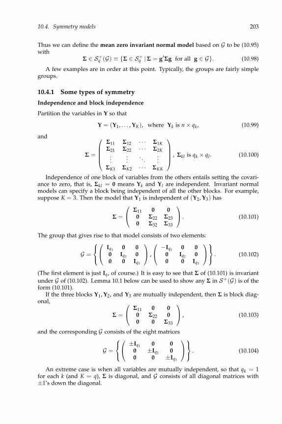
10.4. Symmetry models 203
Thus we can define the mean zero invariant normal model based on G to be (10.95)with
Σ ∈ S+q (G) ≡ Σ ∈ S+
q | Σ = g′Σg for all g ∈ G. (10.98)
A few examples are in order at this point. Typically, the groups are fairly simplegroups.
10.4.1 Some types of symmetry
Independence and block independence
Partition the variables in Y so that
Y = (Y1, . . . , YK), where Yk is n × qk, (10.99)
and
Σ =
Σ11 Σ12 · · · Σ1KΣ21 Σ22 · · · Σ2K
......
. . ....
ΣK1 ΣK2 · · · ΣKK
, Σkl is qk × ql . (10.100)
Independence of one block of variables from the others entails setting the covari-ance to zero, that is, Σkl = 0 means Yk and Yl are independent. Invariant normalmodels can specify a block being independent of all the other blocks. For example,suppose K = 3. Then the model that Y1 is independent of (Y2, Y3) has
Σ =
Σ11 0 00 Σ22 Σ230 Σ32 Σ33
. (10.101)
The group that gives rise to that model consists of two elements:
G =
Iq1 0 00 Iq2 00 0 Iq3
,
−Iq1 0 00 Iq2 00 0 Iq3
. (10.102)
(The first element is just Iq, of course.) It is easy to see that Σ of (10.101) is invariant
under G of (10.102). Lemma 10.1 below can be used to show any Σ in S+(G) is of theform (10.101).
If the three blocks Y1, Y2, and Y3 are mutually independent, then Σ is block diag-onal,
Σ =
Σ11 0 00 Σ22 00 0 Σ33
, (10.103)
and the corresponding G consists of the eight matrices
G =
±Iq1 0 00 ±Iq2 00 0 ±Iq3
. (10.104)
An extreme case is when all variables are mutually independent, so that qk = 1for each k (and K = q), Σ is diagonal, and G consists of all diagonal matrices with±1’s down the diagonal.
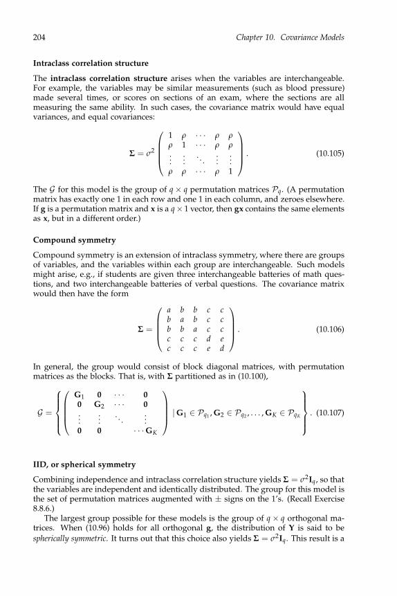
204 Chapter 10. Covariance Models
Intraclass correlation structure
The intraclass correlation structure arises when the variables are interchangeable.For example, the variables may be similar measurements (such as blood pressure)made several times, or scores on sections of an exam, where the sections are allmeasuring the same ability. In such cases, the covariance matrix would have equalvariances, and equal covariances:
Σ = σ2
1 ρ · · · ρ ρρ 1 · · · ρ ρ...
.... . .
......
ρ ρ · · · ρ 1
. (10.105)
The G for this model is the group of q × q permutation matrices Pq. (A permutationmatrix has exactly one 1 in each row and one 1 in each column, and zeroes elsewhere.If g is a permutation matrix and x is a q× 1 vector, then gx contains the same elementsas x, but in a different order.)
Compound symmetry
Compound symmetry is an extension of intraclass symmetry, where there are groupsof variables, and the variables within each group are interchangeable. Such modelsmight arise, e.g., if students are given three interchangeable batteries of math ques-tions, and two interchangeable batteries of verbal questions. The covariance matrixwould then have the form
Σ =
a b b c cb a b c cb b a c cc c c d ec c c e d
. (10.106)
In general, the group would consist of block diagonal matrices, with permutationmatrices as the blocks. That is, with Σ partitioned as in (10.100),
G =
G1 0 · · · 00 G2 · · · 0...
.... . .
...0 0 · · · GK
| G1 ∈ Pq1 , G2 ∈ Pq2 , . . . , GK ∈ PqK
. (10.107)
IID, or spherical symmetry
Combining independence and intraclass correlation structure yields Σ = σ2Iq, so thatthe variables are independent and identically distributed. The group for this model isthe set of permutation matrices augmented with ± signs on the 1’s. (Recall Exercise8.8.6.)
The largest group possible for these models is the group of q × q orthogonal ma-trices. When (10.96) holds for all orthogonal g, the distribution of Y is said to be
spherically symmetric. It turns out that this choice also yields Σ = σ2Iq. This result is a

10.4. Symmetry models 205
reflection of the fact that iid and spherical symmetry are the same for the multivari-ate normal distribution. If Y has some other distribution, then the two models aredistinct, although they still have the same covariance structure.
10.4.2 Characterizing the structure
It is not always obvious given a structure for the covariance matrix to find the cor-responding G , or even to decide whether there is a corresponding G . But given thegroup, there is a straightforward method for finding the structure. We will considerjust finite groups G , but the idea extends to general groups, in which case we wouldneed to introduce uniform (Haar) measure on these groups.
For given finite group G and general Σ, define the G-average of Σ by
Σ =∑g∈G g′
Σg
#G . (10.108)
It should be clear that if Σ ∈ S+q (G), then Σ = Σ. The next lemma shows that all
G-averages are in S+q (G).
Lemma 10.1. For any Σ ∈ S+q , Σ ∈ S+
q (G).
Proof. For any h ∈ G ,
h′Σh =
∑g∈G h′g′Σgh
#G
=∑g∗∈G g∗′
Σg∗
#G= Σ. (10.109)
The second line follows by setting g∗ = gh, and noting that as g runs over G , so doesg∗. (This is where the requirement that G is a group is needed.) But (10.109) implies
that Σ ∈ G .
The lemma shows thatS+
q (G) = Σ | Σ ∈ S+q , (10.110)
so that one can discover the structure of covariance matrices invariant under a partic-ular group by averaging a generic Σ. That is how one finds the structures in (10.101),(10.103), (10.106), and (10.107) from their respective groups.
10.4.3 Maximum likelihood estimates
The maximum likelihood estimate of Σ in (10.98) is the Σ ∈ S+q (G) that maximizes
L(Σ; y) =1
|Σ|n/2e−
12 trace(Σ
−1u), Σ ∈ S+(G), where u = y′y. (10.111)
The requirement Σ ∈ S+q (G) means that
Σ−1 = (g′
Σg)−1 = g′Σ−1g (10.112)

206 Chapter 10. Covariance Models
for any g ∈ G , that is, Σ−1 ∈ S+
q (G), hence
trace(Σ−1u) = trace
(∑g∈G g′
Σ−1g
#G u
)
= trace
(∑g∈G g′
Σ−1gu
#G
)
= trace
(∑g∈G Σ
−1gug′
#G
)
= trace
(Σ−1 ∑g∈G gug′
#G
)
= trace(Σ−1u). (10.113)
Thus
L(Σ; y) =1
|Σ|n/2e−
12 trace(Σ
−1u). (10.114)
We know from Lemma 9.1 that the maximizer of L in (10.114) over Σ ∈ S+q is
Σ =u
n, (10.115)
but since that maximizer is in S+q (G) by Lemma 10.1, and S+
q (G) ⊂ S+q , it must
be the maximizer over S+q (G). That is, (10.115) is indeed the maximum likelihood
estimate for (10.111).To illustrate, let S = U/n. Then if G is as in (10.104), so that the model is that
three sets of variables are independent (10.103), the maximum likelihood estimate isthe sample analog
Σ(G) =
S11 0 00 S22 00 0 S33
. (10.116)
In the intraclass correlation model (10.105), the group is the set of q × q permutationmatrices, and the maximum likelihood estimate has the same form,
Σ(G) = σ2
1 ρ · · · ρρ 1 · · · ρ...
.... . .
...ρ · · · ρ 1
, (10.117)
where
σ2 =1
q
q
∑i=1
sii, and ρσ2 =∑ ∑1≤i<j≤q sij
(q2)
. (10.118)
That is, the common variance is the average of the original variances, and the commoncovariance is the average of the original covariances.

10.4. Symmetry models 207
10.4.4 Hypothesis testing and model selection
The deviance for the model defined by the group G is, by (10.3),
deviance(M(G)) = n log(|Σ(G)|), (10.119)
where we drop the exponential term since nq is the same for all models. We can thenuse this deviance in finding AIC’s or BIC’s for comparing such models, once we figureout the dimensions of the models, which is usually not too hard. E.g., if the model isthat Σ is unrestricted, so that GA = Iq, the trivial group, the dimension for HA isq(q + 1)/2. The dimension for the independence model in (10.103) and (10.104) sumsthe dimensions for the diagonal blocks: q1(q1 + 1)/2 + q2(q2 + 1)/2 + q3(q3 + 1)/2.The dimension for the intraclass correlation model (10.105) is 2 (for the variance andcovariance).
Also, the likelihood ratio statistic for testing two nested invariant normal modelsis easy to find. These testing problems use two nested groups, GA ⊂ G0, so that thehypotheses are
H0 : Σ ∈ S+q (G0) versus HA : Σ ∈ S+
q (GA). (10.120)
Note that the larger G , the smaller S+q (G), since fewer covariance matrices are in-
variant under a larger group. Then the likelihood ratio test statistic, 2 log(LR), is thedifference of the deviances, as in (9.55).
The mean is not zero
So far this subsection assumed the mean of Y is zero. In the more general regressioncase where Y = xβ + R and R ∼ Nn×q(0, In ⊗ Σ), we assume that R is invariant, so
that (10.96) holds for R instead of Y. We estimate Σ restricted to S+q (G) by finding
U = Y′QxY, then taking
Σ =U
nor
U
n − p, (10.121)
(where x is n × p), depending on whether you want the maximum likelihood estimateor an unbiased estimate. In testing, I would suggest taking the unbiased versions,then using
deviance(M(G)) = (n − p) log(|Σ(G)|). (10.122)
10.4.5 Example: Mouth sizes
Continue from Section 7.3.1 with the mouth size data, using the model (7.51). Becausethe measurements within each subject are of the same mouth, a reasonable questionto ask is whether the residuals within each subject are exchangeable, i.e., whether ΣRhas the intraclass correlation structure (10.105). Let U = Y′QxY and the unrestrictedestimate be ΣA = U/ν for ν = n − 2 = 25. Then ΣA and the estimate under theintraclass correlation hypothesis Σ0, given in (10.117) and (10.118), are
ΣA =
5.415 2.717 3.910 2.7102.717 4.185 2.927 3.3173.910 2.927 6.456 4.1312.710 3.317 4.131 4.986
(10.123)
208 Chapter 10. Covariance Models
and
Σ0 =
5.260 3.285 3.285 3.2853.285 5.260 3.285 3.2853.285 3.285 5.260 3.2853.285 3.285 3.285 5.260
. (10.124)
To test the null hypothesis that the intraclass correlation structure holds, versusthe general model, we have from (10.119)
2 log(LR) = 25 (log(|Σ0|)− log(|ΣA|)) = 9.374. (10.125)
The dimension for the general model is dA = q(q + 1)/2 = 10, and for the null isjust d0 = 2, thus the degrees of freedom for this statistic is d f = dA − d0 = 8. Theintraclass correlation structure appears to be plausible.
We can exploit this structure (10.105) on the ΣR to more easily test hypothesesabout the β in both-sides models like (7.51). First, we transform the matrix ΣR into adiagonal matrix with two distinct variances. Notice that we can write this covarianceas
ΣR = σ2(1 − ρ)Iq + σ2ρ1q1′q. (10.126)
Let Γ be any q × q orthogonal matrix whose first column is proportional to 1q, i.e.,1q/
√q. Then
Γ′ΣRΓ = σ2(1 − ρ)Γ′
Γ + σ2ρΓ′1q1′qΓ
= σ2(1 − ρ)Iq + σ2ρ
√q
0...0
( √
q 0 · · · 0)
= σ2
(1 + (q − 1)ρ 0′
0 (1 − ρ)Iq−1
)≡ Λ. (10.127)
We used the fact that because all columns of Γ except the first are orthogonal to 1q,
Γ′1q =
√q(1, 0, . . . , 0)′. As suggested by the notation, this Λ is indeed the eigenvalue
matrix for ΣR (though the diagonals are in a nonincreasing order if ρ < 0), and Γ
contains a corresponding set of eigenvectors.In the model (7.51), the z is almost an appropriate Γ:
z =
1 −3 1 −31 −1 −1 11 1 −1 −11 3 1 3
. (10.128)
The columns are orthogonal, and the first is 14, so we just have to divide each columnby its length to obtain orthonormal columns. The squared lengths of the columns arethe diagonals of z′z : (4, 20, 4, 20). Let ∆ be the square root of z′z,
∆ =
2 0 0 0
0√
20 0 00 0 2 0
0 0 0√
20
, (10.129)
10.4. Symmetry models 209
and setΓ = z∆
−1 and β∗ = β∆, (10.130)
so that the both-sides model can be written
Y = xβ∆∆−1z′ + R = xβ∗
Γ′ + R. (10.131)
Multiplying everything on the right by Γ yields
Y∗ ≡ YΓ = xβ∗ + R∗, (10.132)
whereR∗ ≡ RΓ ∼ N(0, In ⊗ Γ
′ΣRΓ) = N(0, In ⊗ Λ). (10.133)
The estimate of β∗ is straightforward:
β∗ = (x′x)−1x′Y∗ =(
49.938 3.508 0.406 −0.252−4.642 −1.363 −0.429 0.323
). (10.134)
These estimates are the same as those for model (6.29), multiplied by ∆ as in (10.130).The difference is in their covariance matrix:
β∗ ∼ N(β∗, Cx ⊗ Λ). (10.135)
To estimate the standard errors of the estimates, we look at the sum of squaresand cross products of the estimated residuals,
U∗ = Y∗′QxY∗ ∼ Wishartq(ν, Λ), (10.136)
where ν = trace(Qx) = n − p = 27 − 2 = 25. Because the Λ in (10.127) is diagonal,
the diagonals of U∗ are independent scaled χ2ν’s:
U∗11 ∼ τ2
0 χ2ν, U∗
jj ∼ τ21 χ2
ν, j = 2, . . . , q = 4. (10.137)
Unbiased estimates are
τ20 =
U11
ν∼ τ2
0
νχ2
ν and τ21 =
U22 + · · ·Uqq
(q − 1)ν∼ τ2
1
(q − 1)νχ2(q−1)ν. (10.138)
For our data,
τ20 =
377.915
25= 15.117 and τ2
1 =59.167 + 26.041 + 62.919
75= 1.975. (10.139)
The estimated standard errors of the β∗ij’s from (10.135) are found from
Cx ⊗ Λ =
(0.0625 −0.0625
−0.0625 0.1534
)⊗
15.117 0 0 00 1.975 0 00 0 1.975 00 0 0 1.975
, (10.140)
being the square roots of the diagonals:
Standard errorsConstant Linear Quadratic Cubic
Boys 0.972 0.351 0.351 0.351Girls−Boys 1.523 0.550 0.550 0.550
(10.141)
210 Chapter 10. Covariance Models
The t-statistics divide (10.134) by their standard errors:
t-statisticsConstant Linear Quadratic Cubic
Boys 51.375 9.984 1.156 −0.716Girls−Boys −3.048 −2.477 −0.779 0.586
(10.142)
These statistics are not much different from what we found in Section 6.4.1, but thedegrees of freedom for all but the first column are now 75, rather than 25. The mainimpact is in the significance of δ1, the difference between the girls’ and boys’ slopes.Previously, the p-value was 0.033 (the t = −2.26 on 25 df). Here, the p-value is 0.016,a bit stronger suggestion of a difference.
10.5 Exercises
Exercise 10.5.1. Verify the likelihood ratio statistic (10.21) for testing the equality ofseveral covariance matrices as in (10.20).
Exercise 10.5.2. Verify that trace(Σ−1U) = trace(Σ−111 U11) + trace(Σ−1
22 U22), as in(10.27), for Σ being block-diagonal, i.e., Σ12 = 0 in (10.23).
Exercise 10.5.3. Show that the value of 2 log(LR) of (10.30) does not change if the ν’sin the denominators are erased.
Exercise 10.5.4. Suppose U ∼ Wishartq(ν, Σ), where Σ is partitioned as
Σ =
Σ11 Σ12 · · · Σ1KΣ21 Σ22 · · · Σ2K
......
. . ....
ΣK1 ΣK2 · · · ΣKK
, (10.143)
where Σij is qi × qj, and the qi’s sum to q. Consider testing the null hypothesis thatthe blocks are mutually independent, i.e.,
H0 : Σij = 0 for 1 ≤ i < j ≤ K, (10.144)
versus the alternative that Σ is unrestricted. (a) Find the 2 log(LR), and the degrees
of freedom in the χ2 approximation. (The answer is analogous to that in (10.35).) (b)Let U∗ = AUA for some diagonal matrix A with positive diagonal elements. Replacethe U in 2 log(LR) with U∗. Show that the value of the statistic remains the same.(c) Specialize to the case that all qi = 1 for all i, so that we are testing the mutualindependence of all the variables. Let C be the sample correlation matrix. Show that2 log(LR) = −ν log(|C|). [Hint: Find the appropriate A from part (b).]
Exercise 10.5.5. Show that (10.46) holds. [Hint: Apply Exercise 5.8.25(c), with D1 = xand D2 = y3, to obtain
Qx∗ = Qx − Qxy3(y′3Qxy3)
−1y′3Qx. (10.145)
Then show that the right-hand side of (10.46) is the same as V′V, where V is foundby regressing Qxy3 out of Qx(Y1, Y2). This V′V is the left-hand side of (10.46).]

10.5. Exercises 211
Exercise 10.5.6. Show that (10.55) holds.
Exercise 10.5.7. Suppose β and α are both p × q, p < q, and let their decompositionsfrom (10.61) and (10.62) be β = Qβ∗ and α = Γα∗, where Q and Γ are orthogonal,α∗ij = β∗ij = 0 for i > j, and α∗ii’s and β∗ii’s are positive. (We assume the first p columns
of α, and of β, are linearly independent.) Show that α′α = β′β if and only ifα∗ = β∗. [Hint: Use the uniqueness of the QR decomposition, in Theorem 5.4.]
Exercise 10.5.8. Show that the conditional parameters in (10.76) are as in (10.77) and(10.78).
Exercise 10.5.9. Show that if the factor analysis is fit using the correlation matrix,
then the correlation between variable j and factor i is estimated to be βij, the loadingof factor i on variable j.
Exercise 10.5.10. What is the factor analysis model with no factors (i.e., erase the βin (10.57))? Choose from the following: The covariance of Y is unrestricted; the meanof Y is 0; the Y variables are mutually independent; the covariance matrix of Y is aconstant times the identity matrix.
Exercise 10.5.11. Show directly (without using Lemma 10.1) that if Σ ∈ S+q (G) of
(10.98), then Σ in (10.108) is in S+q (G).
Exercise 10.5.12. Verify the steps in (10.113).
Exercise 10.5.13. Show that if Σ has intraclass correlation structure (10.105), thenΣ = σ2(1 − ρ)Iq + σ2ρ1q1′q as in (10.126).
Exercise 10.5.14. Multivariate complex normals arise in spectral analysis of multipletime series. A q-dimensional complex normal is Y1 + i Y2, where Y1 and Y2 are 1 × qreal normal vectors with joint covariance of the form
Σ = Cov[(
Y1 Y2)]
=
(Σ1 F−F Σ1
), (10.146)
i.e., Cov[Y1] = Cov[Y2]. Here, “i” is the imaginary i =√−1. (a) Show that F =
Cov[Y1, Y2] is skew-symmetric, which means that F′ = −F. (b) What is F when q = 1?(c) Show that the set of Σ’s as in (10.146) is the set S+
2q(G) in (10.98) with
G =
I2q,
(0 −Iq
Iq 0
),
(0 Iq
−Ip 0
),−I2q
. (10.147)
(See Andersson and Perlman [1984] for more on this model.)
Exercise 10.5.15 (Mouth sizes). For the boys’ and girls’ mouth size data in Table 4.1,let ΣB be the covariance matrix for the boys’ mouth sizes, and ΣG be the covariancematrix for the girls’ mouth sizes. Consider testing
H0 : ΣB = ΣG versus HA : ΣB 6= ΣG. (10.148)
(a) What are the degrees of freedom for the boys’ and girls’ sample covariance matri-
ces? (b) Find |ΣB|, |ΣG|, and the pooled |Σ|. (Use the unbiased estimates of the Σi’s.)
(c) Find 2 log(LR). What are the degrees of freedom for the χ2? What is the p-value?
Do you reject the null hypothesis (if α = .05)? (d) Look at trace(ΣB), trace(ΣG). Also,look at the correlation matrices for the girls and for the boys. What do you see?

212 Chapter 10. Covariance Models
Exercise 10.5.16 (Mouth sizes). Continue with the mouth size data from Exercise10.5.15. (a) Test whether ΣB has the intraclass correlation structure (versus the general
alternative). What are the degrees of freedom for the χ2? (b) Test whether ΣG hasthe intraclass correlation structure. (c) Now assume that both ΣB and ΣG have theintraclass correlation structure. Test whether the covariance matrices are equal. Whatare the degrees of freedom for this test? What is the p-value? Compare this p-valueto that in Exercise 10.5.15, part (c). Why is it so much smaller (if it is)?
Exercise 10.5.17 (Grades). This problem considers the grades data. In what follows,use the pooled covariance matrix in (10.18), which has ν = 105. (a) Test the indepen-dence of the first three variables (homework, labs, inclass) from the fourth variable,the midterms score. (So leave out the final exams at this point.) Find l1, l2, |Σ11|, |Σ22|,and |Σ|. Also, find 2 log(LR) and the degrees of freedom for the χ2. Do you accept orreject the null hypothesis? (b) Now test the conditional independence of the set (home-work, labs, inclass) from the midterms, conditioning on the final exam score. What
is the ν for the estimated covariance matrix now? Find the new l1, l2, |Σ11|, |Σ22|, and
|Σ|. Also, find 2 log(LR) and the degrees of freedom for the χ2. Do you accept orreject the null hypothesis? (c) Find the correlations between the homework, labs andinclass scores and the midterms scores, as well as the conditional correlations giventhe final exam. What do you notice?
Exercise 10.5.18 (Grades). The table in (10.93) has the BIC’s for the one-factor, two-factor, and unrestricted models for the grades data. Find the deviance, dimension,and BIC for the zero-factor model, M0. (See Exercise 10.5.10.) Find the estimatedprobabilities of the four models. Compare the results to those without M0.
Exercise 10.5.19 (Exams). The exams matrix has data on 191 statistics students, givingtheir scores (out of 100) on the three midterm exams and the final exam. (a) Whatis the maximum number of factors that can be estimated? (b) Give the number ofparameters in the covariance matrices for the 0, 1, 2, and 3 factor models (even if theyare not estimable). (c) Plot the data. There are three obvious outliers. Which obser-vations are they? What makes them outliers? For the remaining exercise, eliminatethese outliers, so that there are n = 188 observations. (d) Test the null hypothesisthat the four exams are mutually independent. What are the adjusted 2 log(LR)∗
(in (10.70)) and degrees of freedom for the χ2? What do you conclude? (e) Fit theone-factor model. What are the loadings? How do you interpret them? (f) Look at
the residual matrix C − β′β, where C is the observed correlation matrix of the orig-inal variables. If the model fits exactly, what values would the off-diagonals of theresidual matrix be? What is the largest off-diagonal in this observed matrix? Are thediagonals of this matrix the uniquenesses? (g) Does the one-factor model fit?
Exercise 10.5.20 (Exams). Continue with the Exams data from Exercise 10.5.19. Again,do not use the outliers found in part (c). Consider the invariant normal model wherethe group G consists of 4 × 4 matrices of the form
G =
(G∗ 0′303 1
)(10.149)
where G∗ is a 3 × 3 permutation matrix. Thus the model is an example of compoundsymmetry, from Section 10.4.1. The model assumes the three midterms are inter-changeable. (a) Give the form of a covariance matrix Σ that is invariant under that G .

10.5. Exercises 213
(It should be like the upper-left 4 × 4 block of the matrix in (10.106).) How many freeparameters are there? (b) For the exams data, give the MLE of the covariance matrixunder the assumption that it is G-invariant. (c) Test whether this symmetry assump-tion holds, versus the general model. What are the degrees of freedom? For whichelements of Σ is the null hypothesis least tenable? (d) Assuming Σ is G-invariant,test whether the first three variables are independent of the last. (That is, the nullhypothesis is that Σ is G-invariant and σ14 = σ24 = σ34 = 0, while the alternative isthat Σ is G-invariant, but otherwise unrestricted.) What are the degrees of freedomfor this test? What do you conclude?
Exercise 10.5.21 (South Africa heart disease). The data for this question comes froma study of heart disease in adult males in South Africa from Rossouw et al. [1983].(We return to these data in Section 11.8.) The R data frame is SAheart, found inthe ElemStatLearn package [Halvorsen, 2012]. The main variable of interest is “chd,”congestive heart disease, where 1 indicates the person has the disease, 0 he doesnot. Explanatory variables include sbc (measurements on blood pressure), tobaccouse, ldl (bad cholesterol), adiposity (fat %), family history of heart disease (absentor present), type A personality, obesity, alcohol usage, and age. Here you are tofind common factors among the the explanatory variables excluding age and familyhistory. Take logs of the variables sbc, ldl, and obesity, and cube roots of alcoholand tobacco, so that the data look more normal. Age is used as a covariate. ThusY is n × 7, and D = (1n xage). Here, n = 462. (a) What is there about the tobaccoand alcohol variables that is distinctly non-normal? (b) Find the sample correlationmatrix of the residuals from the Y = Dγ + R model. Which pairs of variables havecorrelations over 0.25, and what are their correlations? How would you group thesevariables? (c) What is the largest number of factors that can be fit for this Y? (d) Givethe BIC-based probabilities of the p-factor models for p = 0 to the maximum foundin part (c), and for the unrestricted model. Which model has the highest probability?
Does this model fit, according to the χ2 goodness of fit test? (e) For the most probablemodel from part (d), which variables’ loadings are highest (over 0.25) for each factor?(Use the varimax rotation for the loadings.) Give relevant names to the two factors.Compare the factors to what you found in part (b). (f) Keeping the same model,find the estimated factor scores. For each factor, find the two-sample t-statistic forcomparing the people with heart disease to those without. (The statistics are notactually distributed as Student’s t, but do give some measure of the difference.) (g)Based on the statistics in part (f), do any of the factors seem to be important factors inpredicting heart disease in these men? If so, which one(s). If not, what are the factorsexplaining?
Exercise 10.5.22 (Decathlon). Exercise 1.9.22 created a biplot for the decathlon data.The data consist of the scores (number of points) on each of ten events for the top 24men in the decathlon at the 2008 Olympics. For convenience, rearrange the variablesso that the running events come first, then the jumping, then throwing (ignoring theoverall total):
y <− decathlon[,c(1,5,10,6,3,9,7,2,4,8)]
Fit the 1, 2, and 3 factor models. (The chi-squared approximations for the fit mightnot be very relevant, because the sample size is too small.) Based on the loadings, canyou give an interpretation of the factors? Based on the uniquenesses, which eventsseem to be least correlated with the others?


Chapter 11
Classification
Multivariate analysis of variance seeks to determine whether there are differencesamong several groups, and what those differences are. Classification is a related areain which one uses observations whose group memberships are known in order toclassify new observations whose group memberships are not known. This goal wasthe basic idea behind the gathering of the Fisher-Anderson iris data (Section 1.3.1).Based on only the petal and sepal measurements of a new iris, can one effectivelyclassify it into one of the three species setosa, virginica, and versicolor? See Figure1.4 for an illustration of the challenge.
The task is prediction, as in Section 7.5, except that rather than predicting a con-tinuous variable Y, we predict a categorical variable. We will concentrate mainly onlinear methods arising from Fisher’s methods, logistic regression, and trees. There isa vast array of additional approaches, including using neural networks, support vec-tor machines, boosting, bagging, and a number of other flashy-sounding techniques.
Related to classification is clustering (Chapter 12), in which one assumes that thereare groups in the population, but which groups the observations reside in is unob-served, analogous to the factors in factor analysis. In the machine learning com-munity, classification is supervised learning, because we know the groups and havesome data on group membership, and clustering is unsupervised learning, becausegroup membership itself must be estimated. See the book by Hastie, Tibshirani, andFriedman [2009] for a fine statistical treatment of machine learning.
The basic model is a mixture model, presented in the next section.
11.1 Mixture models
The mixture model we consider assumes there are K groups, numbered from 1 to K,and p predictor variables on which to base the classifications. The data then consistof n observations, each a 1 × (p + 1) vector,
(Xi, Yi), i = 1, . . . , n, (11.1)
where Xi is the 1× p vector of predictors for observation i, and Yi is the group numberof observation i, so that Yi ∈ 1, . . . , K. Marginally, the proportion of the populationin group k is
P[Y = k] = πk, k = 1, . . . , K. (11.2)
215

216 Chapter 11. Classification
0 5 10 15
0.0
0.1
0.2
0.3
0.4
x
Figure 11.1: Three densities, plus a mixture of the three (the thick line).
Each group then has a conditional distribution Pk:
Xi |Yi = k ∼ Pk , (11.3)
where the Pk will (almost always) depend on some unknown parameters. Assumingthat Pk has density fk(x), the joint density of (Xi, Yi) is a mixed one as in (2.11), with
f (xi, yi) = fyi(xi)πyi
. (11.4)
The marginal pdf of Xi is found by summing the joint density over the groups:
f (xi) = π1 f1(xi) + · · ·+ πK fK(xi). (11.5)
For example, suppose that K = 3, π1 = π2 = π3 = 1/3, and the three groups are,conditionally,
X |Y = 1 ∼ N(5, 1), X |Y = 2 ∼ N(5, 22), X |Y = 3 ∼ N(10, 1). (11.6)
Figure 11.1 exhibits the three pdfs, plus the mixture pdf, which is the thick black line.The data for classification includes the group index, so that the joint distributions
of (Xi, Yi) are operative, meaning we can estimate the individual densities. The over-all density for the data is then
n
∏i=1
f (xi, yi) =n
∏i=1
fyi(xi)πyi
=
πN1
1 ∏i|yi=1
f1(xi)
· · ·
πNK
K ∏i|yi=K
fK(xi)
=
[K
∏k=1
πNk
k
]×
K
∏k=1
∏i|yi=k
fk(xi)
, (11.7)
11.2. Classifiers 217
where Nk is the number of observations in group k:
Nk = #yi = k. (11.8)
The classification task arises when a new observation, XNew, arrives without its group
identification YNew, so its density is that of the mixture. We have to guess what thegroup is.
In clustering, the data themselves are without group identification, so we have justthe marginal distributions of the Xi. Thus the joint pdf for the data is
Πni=1 f (xi) = Πn
i=1(π1 f1(xi) + · · ·+ πK fK(xi)). (11.9)
Thus clustering is similar to classifying new observations, but without having anyprevious y data to help estimate the πk’s and fk’s. See Section 12.3.
11.2 Classifiers
A classifier is a function C that takes the new observation, and emits a guess at itsgroup:
C : X −→ 1, . . . , K, (11.10)
where X is the space of XNew. The classifier may depend on previous data, as well
as on the πk’s and fk’s, but not on the YNew. A good classifier is one that is unlikelyto make a wrong classification. Thus a reasonable criterion for a classifier is theprobability of an error:
P[C(XNew) 6= YNew]. (11.11)
We would like to minimize that probability. (This criterion assumes that any type ofmisclassification is equally bad. If that assumption is untenable, then one can use aweighted probability:
K
∑k=1
K
∑l=1
wklP[C(XNew) = k and YNew = l], (11.12)
where wkk = 0.)Under the (unrealistic) assumption that we know the πk’s and fk’s, the best guess
of YNew given XNew is the group that has the highest conditional probability.
Lemma 11.1. Define the Bayes classifier by
CB(x) = k i f P[Y = k | X = x] > P[Y = l | X = x] f or l 6= k. (11.13)
Then CB minimizes (11.11) over classifiers C.
Proof. Let I be the indicator function, so that
I[C(XNew) 6= YNew] =
1 i f C(XNew) 6= YNew
0 i f C(XNew) = YNew (11.14)
and
P[C(XNew) 6= YNew] = E[I[C(XNew) 6= YNew]]. (11.15)

218 Chapter 11. Classification
As in (2.34), we have that
E[I[C(XNew) 6= YNew]] = E[eI(XNew)], (11.16)
where
eI(xNew) = E[I[C(XNew) 6= YNew] | XNew = xNew]
= P[C(xNew) 6= YNew | XNew = xNew]
= 1 − P[C(xNew) = YNew |XNew = xNew]. (11.17)
Thus if we minimize the last expression in (11.17) for each xNew, we have minimizedthe expected value in (11.16). Minimizing (11.17) is the same as maximizing
P[C(xNew) = YNew | XNew = xNew], (11.18)
but that conditional probability can be written
K
∑l=1
I[C(xNew) = l] P[YNew = l | XNew = xNew]. (11.19)
This sum equals P[YNew = l | XNew = xNew] for whichever k C chooses, so to maxi-mize the sum, choose the l with the highest conditional probability, as in (11.13).
Now the conditional distribution of YNew given XNew is obtained from (11.4) and(11.5) (it is Bayes theorem, Theorem 2.2):
P[YNew = k | XNew = xNew] =fk(x
New)πk
f1(xNew)π1 + · · ·+ fK(xNew)πK. (11.20)
Since, given xNew, the denominator is the same for each k, we just have to choose thek to maximize the numerator:
CB(x) = k if fk(xNew)πk > fl(x
New)πl f or l 6= k. (11.21)
We are assuming there is a unique maximum, which typically happens in practicewith continuous variables. If there is a tie, any of the top categories will yield theoptimum.
Consider the example in (11.6). Because the πk’s are equal, it is sufficient to look atthe conditional pdfs. A given x is then classified into the group with highest density,as given in Figure 11.2. Thus the classifications are
CB(x) =
1 if 3.640 < x < 6.3602 if x < 3.640 or 6.360 < x < 8.067 or x > 15.2673 if 8.067 < x < 15.267.
(11.22)
In practice, the πk’s and fk’s are not known, but can be estimated from the data.Consider the joint density of the data as in (11.7). The πk’s appear in only the firstterm. They can be estimated easily (as in a multinomial situation) by
πk =Nk
n. (11.23)
The parameters for the fk’s can be estimated using the xi’s that are associated withgroup k. These estimates are then plugged into the Bayes formula to obtain an ap-proximate Bayes classifier. The next section shows what happens in the multivariatenormal case.

11.3. Linear discrimination 219
0 5 10 15
0.0
0.1
0.2
0.3
0.4
2 1 2 3
x
Figure 11.2: Three densities, and the regions in which each is the highest. The den-sities are 1: N(5,1), solid line; 2: N(5,4), dashed line; 3: N(10,1), dashed/dotted line.Density 2 is also the highest for x > 15.267.
11.3 Fisher’s linear discrimination
Suppose that the individual fk’s are multivariate normal densities with differentmeans but the same covariance, so that
Xi |Yi = k ∼ N1×p(µk , Σ). (11.24)
The pdf’s (8.47) are then
fk(x |µk, Σ) = c1
|Σ|1/2e−
12 (x−µk)Σ
−1(x−µk)′
= c1
|Σ|1/2e−
12 xΣ
−1x′exΣ
−1µ′k− 1
2µkΣ−1µ′
k . (11.25)
We can ignore the factors that are the same for each group, i.e., that do not dependon k, because we are in quest of the highest pdf×πk. Thus for a given x, we choosethe k to maximize
πk exΣ−1µ′
k− 12µkΣ
−1µ′k , (11.26)
or, by taking logs, the k that maximizes
d∗k (x) ≡ xΣ−1µ′
k −1
2µkΣ
−1µ′k + log(πk). (11.27)
These d∗k ’s are called the discriminant functions. Note that in this case, they arelinear in x, hence linear discriminant functions. It is often convenient to target one
group (say the Kth) as a benchmark, then use the functions
dk(x) = d∗k (x)− d∗K(x), (11.28)
220 Chapter 11. Classification
so that the final function is 0.We still must estimate the parameters, but that task is straightforward: take the
πk = NK/n as in (11.23), estimate the µk’s by the obvious sample means:
µk =1
Nk∑
i|yi=kxi, (11.29)
and estimate Σ by the MLE, i.e., because we are assuming the covariances are equal,the pooled covariance:
Σ =1
n
K
∑k=1
∑i|yi=k
(xi − µk)′(xi − µk). (11.30)
(The numerator equals X′(In − P)X for P being the projection matrix for the designmatrix indicating which groups the observations are from. We could divide by n − Kto obtain the unbiased estimator, but the classifications would still be essentially thesame, exactly so if the πk’s are equal.) Thus the estimated discriminant functions are
dk(x) = ck + xa′k , (11.31)
where
ak = (µk − µK)Σ−1
and
ck = − 1
2(µkΣ
−1µ′
k − µKΣ−1µ′
K) + log(πk/πK). (11.32)
Now we can define the classifier based upon Fisher’s linear discrimination func-tion to be
CFLD(x) = k i f dk(x) > dl(x) f or l 6= k. (11.33)
(The hat is there to emphasize the fact that the classifier is estimated from the data.) Ifp = 2, each set x | dk(x) = dl(x) defines a line in the x-space. These lines divide thespace into a number of polygonal regions (some infinite). Each region has the same
C(x). Similarly, for general q, the regions are bounded by hyperplanes. Figure 11.3illustrates for the iris data when using just the sepal length and width. The solid lineis the line for which the discriminant functions for setosas and versicolors are equal.It is basically perfect for these data. The dashed line tries to separate setosas andvirginicas. There is one misclassification. The dashed/dotted line tries to separatethe versicolors and virginicas. It is not particularly successful. See Section 11.4.1 fora better result using all the variables.
Remark
Fisher’s original derivation in Fisher [1936] of the classifier (11.33) did not start withthe multivariate normal density. Rather, in the case of two groups, he obtained thep × 1 vector a that maximized the ratio of the squared difference of means of thevariable Xia
′ for the two groups to the variance:
((µ1 − µ2)a′)2
aΣa′. (11.34)

11.4. Cross-validation estimate of error 221
s
ss
s
s
s
s s
ss
s
s
ss
s
s
s
s
ss
s
ss
ss
s
sss
ss
s
ss
ss
ss
s
ss
s
s
s
s
s
s
s
s
svv
v
v
vv
v
v
vv
v
v
v
vvv
v
v
v
v
v
v
v
vv
vv
vv
vvv
v v
v
v
v
v
v
vv
v
v
v
v
vv v
v
v
g
g
gg
g g
g
g
g
g
g
g
g
g
g
gg
g
g
g
g
g gg
gg
gg
gg
g
g
ggg
g
g
gg
gg g
g
gg
g
g
g
g
g
4.5 5.5 6.5 7.5
2.0
2.5
3.0
3.5
4.0
Sepal length
Sep
al w
idth
Figure 11.3: Fisher’s linear discrimination for the iris data using just sepal lengthand width. The solid line separates setosa (s) and versicolor (v); the dashed lineseparates setosa and virginica (g); and the dashed/dotted line separates versicolorand virginica.
The optimal a is (anything proportional to)
a = (µ1 − µ2)Σ−1
, (11.35)
which is the a1 in (11.32). Even though our motivation leading to (11.27) is differentthan Fisher’s, because we end up with his coefficients, we will refer to (11.31) asFisher’s.
11.4 Cross-validation estimate of error
In classification, an error occurs if an observation is misclassified, so one often usesthe criterion (11.11) to assess the efficacy of a classifier. Since we are estimating theclassifier, we wish to find
ClassError = P[C(XNew) 6= YNew]. (11.36)
This probability takes into account the dependence of the estimated classifier on the
data, as well as on the randomness of (XNew, YNew), assumed to be independent ofthe data. How does one estimate the error? The obvious approach is to try theclassifier on the data, and count the number of misclassifications:
ClassErrorObs =1
n
n
∑i=1
I[C(xi) 6= yi]. (11.37)
222 Chapter 11. Classification
As in prediction, this error will be an underestimate because we are using the samedata to estimate the classifier and test it out. A common approach to a fair estimateis to initially set aside a randomly chosen fraction of the observations (e.g., 10% to25%) to be test data, and use the remaining so-called training data to estimate theclassifier. Then this estimated classifier is tested on the test data.
Cross-validation is a method that takes the idea one step further, by repeatedlyseparating the data into test and training data. The “leave-one-out” cross-validationuses single observations as the test data. It starts by setting aside the first observation,(x1, y1), and calculating the classifier using the data (x2, y2), . . . , (xn, yn). (That is, wefind the sample means, covariances, etc., leaving out the first observation.) Call the
resulting classifier C(−1). Then determine whether this classifier classifies the firstobservation correctly:
I[C(−1)(x1) 6= y1]. (11.38)
The C(−1) and (X1, Y1) are independent, so the function in (11.38) is almost an unbi-ased estimate of the error in (11.36). The only reason it is not exactly unbiased is that
C(−1) is based on n − 1 observations, rather than the n for C . This difference shouldbe negligible.
Repeat the process, leaving out each observation in turn, so that C(−i) is the classi-fier calculated without observation i. Then the almost unbiased estimate of ClassErrorin (11.36) is
ClassErrorLOOCV =1
n
n
∑i=1
I[C(−i)(xi) 6= yi]. (11.39)
If n is large, and calculating the classifier is computationally challenging, then leave-one-out cross-validation can use up too much computer time (especially if one istrying a number of different classifiers). Also, the estimate, though nearly unbiased,might have a high variance. An alternative is to leave out more than one observationeach time, e.g., the 10% cross-validation would break the data set into 10 test sets ofsize ≈ n/10, and for each set, use the other 90% to estimate the classifier to use on thetest set. This approach is much more computationally efficient, and less variable, butdoes introduce more bias. Kshirsagar [1972] contains a number of other suggestionsfor estimating the classification error.
11.4.1 Example: Iris data
Turn again to the iris data. Figure 1.3 has the scatter plot matrix. Also see Figures1.4 and 11.3. In R, the iris data is in the data frame iris. You may have to load thedatasets package. The first four columns constitute the n × p matrix of xi’s, n = 150,p = 4. The fifth column has the species, 50 each of setosa, versicolor, and virginica.The basic variables are then
x.iris <− as.matrix(iris[,1:4])y.iris <− rep(1:3,c(50,50,50)) # gets group vector (1,...,1,2,...,2,3,...,3)
We will offload many of the calculations to the function lda in Section A.3.1. Thefollowing statement calculates the ak and ck in (11.32):
ld.iris <− lda(x.iris,y.iris)
11.4. Cross-validation estimate of error 223
The ak are in the matrix ld.iris$a and the ck are in the vector ld.iris$c, given below:
k ak ck
1 (Setosa) 11.325 20.309 −29.793 −39.263 18.4282 (Versicolor) 3.319 3.456 −7.709 −14.944 32.1593 (Virginica) 0 0 0 0 0
(11.40)
Note that the final coefficients are zero, because of the way we normalize the functionsin (11.28).
To see how well the classifier works on the data, we have to first calculate thedk(xi). The following places these values in an n × K matrix disc:
disc <− x.iris%∗%ld.iris$adisc <− sweep(disc,2,ld.iris$c,’+’)
The rows corresponding to the first observation from each species are
ki 1 2 31 97.703 47.400 0
51 −32.305 9.296 0101 −120.122 −19.142 0
(11.41)
The classifier (11.33) classifies each observation into the group corresponding to thecolumn with the largest entry. Applied to the observations in (11.41), we have
CFLD(x1) = 1, CFLD(x51) = 2, CFLD(x101) = 3, (11.42)
that is, each of these observations is correctly classified into its group. To find the
CFLD’s for all the observations, use
imax <− function(z) ((1:length(z))[z==max(z)])[1]yhat <− apply(disc,1,imax)
where imax is a little function to give the index of the largest value in a vector. To seehow close the predictions are to the observed, use the table command:
table(yhat,y.iris)
which yieldsy
y 1 2 31 50 0 02 0 48 13 0 2 49
(11.43)
Thus there were 3 observations misclassified — two versicolors were classified asvirginica, and one virginica was classified as versicolor. Not too bad. The observedmisclassification rate is
ClassErrorObs =#CFLD(xi) 6= yi
n=
3
150= 0.02. (11.44)
As noted above in Section 11.4, this value is likely to be an optimistic estimate (anunderestimate) of ClassError in (11.36), because it uses the same data to find the clas-sifier and to test it out. We will find the leave-one-out cross-validation estimate (11.39)using the code below, where we set varin=1:4 to specify using all four variables.

224 Chapter 11. Classification
yhat.cv <− NULLn <− nrow(x.iris)for(i in 1:n)
dcv <− lda(x.iris[−i,varin],y.iris[−i])dxi <− x.iris[i,varin]%∗%dcv$a+dcv$cyhat.cv <− c(yhat.cv,imax(dxi))
sum(yhat.cv!=y.iris)/n
Here, for each i, we calculate the classifier without observation i, then apply it tothat left-out observation i, the predictions placed in the vector yhat.cv. We then count
how many observations were misclassified. In this case, ClassErrorLOOCV = 0.02,just the same as the observed classification error. In fact, the same three observationswere misclassified.
Subset selection
The above classifications used all four iris variables. We now see if we can obtainequally good or better results using a subset of the variables. We use the same loopas above, setting varin to the vector of indices for the variables to be included. Forexample, varin = c(1,3) will use just variables 1 and 3, sepal length and petal length.
Below is a table giving the observed error and leave-one-out cross-validation error(in percentage) for 15 models, depending on which variables are included in theclassification.
Classification errorsVariables Observed Cross-validation
1 25.3 25.32 44.7 48.03 5.3 6.74 4.0 4.0
1, 2 20.0 20.71, 3 3.3 4.01, 4 4.0 4.72, 3 4.7 4.72, 4 3.3 4.03, 4 4.0 4.0
1, 2, 3 3.3 4.01, 2, 4 4.0 5.31, 3, 4 2.7 2.72, 3, 4 2.0 4.0
1, 2, 3, 4 2.0 2.0
(11.45)
Note that the cross-validation error estimates are either the same, or a bit larger,than the observed error rates. The best classifier uses all 4 variables, with an estimated2% error. Note, though, that variable 4 (petal width) alone has only a 4% error rate.Also, adding variable 1 to variable 4 actual worsens the prediction a little, showingthat adding the extra variation is not worth it. Looking at just the observed error, theprediction stays the same.
Figure 11.4 shows the classifications using just petal widths. Because the samplesizes are equal, and the variances are assumed equal, the separating lines between

11.5. Quadratic discrimination 225
setosa versicolor virginica
0.5
1.0
1.5
2.0
2.5
Pet
al w
idth
Figure 11.4: Boxplots of the petal widths for the three species of iris. The solidline separates the setosas from the versicolors, and the dashed line separates theversicolors from the virginicas.
two species are just the average of their means. We did not plot the line for setosaversus virginica. There are six misclassifications, two versicolors and four virginicas.(Two of the latter had the same petal width, 1.5.)
11.5 Fisher’s quadratic discrimination
When the equality of the covariance matrices is not tenable, we can use a slightlymore complicated procedure. Here the conditional probabilities are proportional to
πk fk(x |µk, Σk) = c πk1
|Σk|1/2e−
12 (x−µk)Σ
−1k (x−µk)
′
= c e−12 (x−µk)Σ
−1k (x−µk)
′− 12 log(|Σk |)+log(πk). (11.46)
Then the discriminant functions can be taken to be the terms in the exponents (times2, for convenience), or their estimates:
d Qk (x) = −(x − µk)Σ
−1k (x − µk)
′ + ck, (11.47)
whereck = − log(|Σk|) + 2 log(Nk/n), (11.48)
and Σk is the sample covariance matrix from the kth group. Now the boundariesbetween regions are quadratic rather than linear, hence Fisher’s quadratic discrimi-nation function is defined to be
CFQD(x) = k i f d Qk (x) > d Q
l (x) f or l 6= k. (11.49)

226 Chapter 11. Classification
11.5.1 Example: Iris data, continued
We consider the iris data again, but as in Section 11.5 we estimate three separate co-variance matrices. Sections A.3.2 and A.3.3 contain the functions qda and predict_qdafor calculating the quadratic discriminant functions (11.25) and finding the predic-tions. Apply these to the iris data as follows:
qd.iris <− qda(x.iris,y.iris)yhat.qd <− NULLfor (i in 1:n)
yhat.qd <− c(yhat.qd,imax(predict_qda(qd.iris,x.iris[i,])))table(yhat.qd,y.iris)
The resulting table is (11.43), the same as for linear discrimination. The leave-one-outcross-validation estimate of classification error is 4/150 = 0.0267, which is slightlyworse than that for linear discrimination. It does not appear that the extra complica-tion of having three covariance matrices improves the classification rate.
Hypothesis testing, AIC, or BIC can also help decide between the model with equalcovariance matrices and the model with three separate covariance matrices. Becausewe have already calculated the estimates, it is quite easy to proceed. The two modelsare then
MSame ⇒ Σ1 = Σ2 = Σ3 ≡ Σ;
MDiff ⇒ (Σ1, Σ2, Σ3) unrestricted. (11.50)
Both models have the same unrestricted means, and we can consider the πk’s fixed,so we can work with just the sample covariance matrices, as in Section 10.1. LetU1, U2, and U3 be the sum of squares and cross-products matrices (1.15) for the threespecies, and U = U1 + U2 + U3 be the pooled version. The degrees of freedom foreach species is νk = 50 − 1 = 49. Thus from (10.10) and (10.11), we can find thedeviances (9.53) to be
deviance(MSame) = (ν1 + ν2 + ν3) log(|U/(ν1 + ν2 + ν3)|)= −1463.905,
deviance(MDiff) = ν1 log(|U1/ν1|) + ν2 log(|U2/ν2|) + ν3 log(|U3/ν3|)= −1610.568 (11.51)
Each covariance matrix has q(q + 1)/2 = 10 parameters, hence
dSame = 10 and dDiff = 30. (11.52)
To test the null hypothesis MSame versus the alternative MDiff, as in (9.55),
2 log(LR) = deviance(MSame)− deviance(MDiff)
= −1463.905 + 1610.568
= 146.663, (11.53)
on dSame − dDiff = 20 degrees of freedom. The statistic is highly significant; we reject
emphatically the hypothesis that the covariance matrices are the same. The AIC’s

11.6. Modifications 227
(9.56) and BIC’s (9.57) are found directly from (11.53):
AIC BICMSame −1443.90 −1414.00MDiff −1550.57 −1460.86
(11.54)
They, too, favor the separate covariance model. Cross-validation above suggests thatthe equal-covariance model is slightly better. Thus there seems to be a conflict be-tween AIC/BIC and cross-validation. The conflict can be explained by noting thatAIC/BIC are trying to model the distribution of the (xi, yi)’s, while cross-validationdoes not really care about the distribution of the xi’s, except to the extent it helps inpredicting the yi’s.
11.6 Modifications to Fisher’s discrimination
The key component in both the quadratic and linear discriminant functions is thequadratic form,
q(x;µk, ΣK) = − 1
2(x −µk)Σ
−1k (x −µk)
′, (11.55)
where in the case the Σk’s are equal, the “xΣ−1x′” part is ignored. Without the −1/2,
(11.55) is a measure of distance (called the Mahalanobis distance) between an x andthe mean of the kth group, so that it makes sense to classify an observation into thegroup to which it is closest (modulo an additive constant). The idea is plausiblewhether the data are normal or not, and whether the middle component is a generalΣk or not. E.g., when taking the Σ’s equal, we could take
Σ = Ip =⇒ q(x;µk, Ip) = − 1
2‖x −µk‖2, or
Σ = ∆, diagonal =⇒ q(x;µk, ∆) = − 1
2 ∑(xi −µki)2/δii. (11.56)
The first case is regular Euclidean distance. In the second case, one would need toestimate the δii’s by the pooled sample variances. These alternatives may be betterwhen there are not many observations per group, and a fairly large number of vari-ables p, so that estimating a full Σ introduces enough extra random error into theclassification to reduce its effectiveness.
Another modification is to use functions of the individual variables. E.g., in theiris data, one could generate quadratic boundaries by using the variables
Sepal Length, (Sepal Length)2, Petal Length, (Petal Length)2 (11.57)
in the x. The resulting set of variables certainly would not be multivariate normal,but the classification based on them may still be reasonable. See the next section foranother method of incorporating such functions.
11.7 Conditioning on X: Logistic regression
Based on the conditional densities of X given Y = k and priors πk, Lemma 11.1shows that the Bayes classifier in (11.13) is optimal. In Section 11.3, we saw that if the
228 Chapter 11. Classification
conditional distributions of the X are multivariate normal, with the same covariancematrix for each group, then the classifier devolved to a linear one (11.31) in x. Thelinearity is not specific to the normal, but is a consequence of the normal being anexponential family density, which means the density has the form
f (x |θ) = a(x)et(x)θ′−ψ(θ) (11.58)
for some 1× m parameter θ, 1× m function t(x) (the sufficient statistic), and functiona(x), where ψ(θ) is the normalizing constant.
Suppose that the conditional density of X given Y = k is f (x | θk), that is, eachgroup has the same form of the density, but a different parameter value. Then theanalog to equations (11.27) and (11.28) yields discriminant functions like those in(11.31),
dk(x) = γk + t(x)α′k, (11.59)
a linear function of t(x), where αk = θk − θK, and γk is a constant depending on theparameters. (Note that dK(x) = 0.) To implement the classifier, we need to estimatethe parameters θk and πk, usually by finding the maximum likelihood estimates.(Note that Fisher’s quadratic discrimination in Section 11.5 also has discriminantfunctions (11.47) of the form (11.59), where the t is a function of the x and its square,xx′.) In such models the conditional distribution of Y given X is given by
P[Y = k |X = x] =edk(x)
ed1(x) + · · ·+ edK−1(x) + 1(11.60)
for the dk’s in (11.59). This conditional model is called the logistic regression model.Then an alternative method for estimating the γk’s and αk’s is to find the values thatmaximize the conditional likelihood,
L((γ1,α1), . . . , (γK−1,αK−1) ; (x1, y1), . . . , (xn, yn)) =n
∏i=1
P[Y = yi | Xi = xi]. (11.61)
(We know that αK = 0 and γK = 0.) There is no closed-form solution for solvingthe likelihood equations, so one must use some kind of numerical procedure likeNewton-Raphson. Note that this approach estimates the slopes and intercepts of thediscriminant functions directly, rather than (in the normal case) estimating the meansand variances, and the πk’s, then finding the slopes and intercepts as functions ofthose estimates.
Whether using the exponential family model unconditionally or the logistic modelconditionally, it is important to realize that both lead to the exact same theoreticalclassifier. The difference is in the way the slopes and intercepts are estimated in(11.59). One question is then which gives the better estimates. Note that the jointdistribution of the (X, Y) is the product of the conditional of Y given X in (11.60) andthe marginal of X in (11.5), so that for the entire data set,
n
∏i=1
f (yi, xi | θk)πyi=
[n
∏i=1
P[Y = yi | Xi = xi, θk]
]
×[
n
∏i=1
(π1 f (xi | θ1) + · · ·+ πK f (xi | θK))
].
(11.62)
11.7. Logistic regression 229
Thus using just the logistic likelihood (11.61), which is the first term on the right-hand side in (11.62), in place of the complete likelihood on the left, leaves out theinformation about the parameters that is contained in the mixture likelihood (thesecond term on the right). As we will see in Chapter 12, there is information in themixture likelihood. One would then expect that the complete likelihood gives betterestimates in the sense of asymptotic efficiency of the estimates. It is not clear whetherthat property always translates to yielding better classification schemes, but maybe.
On the other hand, the conditional logistic model is more general in that it yieldsvalid estimates even when the exponential family assumption does not hold. We canentertain the assumption that the conditional distributions in (11.60) hold for anystatistics t(x) we wish to use, without trying to model the marginal distributions ofthe X’s at all. This realization opens up a vast array of models to use, that is, we cancontemplate any functions t we wish.
In what follows, we restrict ourselves to having K = 2 groups, and renumber thegroups 0, 1, so that Y is conditionally Bernoulli:
Yi | Xi = xi ∼ Bernoulli(ρ(xi)), (11.63)
where
ρ(x) = P[Y = 1 | X = x]. (11.64)
The modeling assumption from (11.60) can be translated to the logit (log odds) of ρ,logit(ρ) = log(ρ/(1 − ρ)). Then
logit(ρ(x)) = logit(ρ(x |γ,α)) = γ + xα′. (11.65)
(We have dropped the t from the notation. You can always define x to be whateverfunctions of the data you wish.) The form (11.65) exhibits the reason for calling themodel “logistic regression.” Letting
logit(ρ) =
logit(ρ(x1 | γ,α))logit(ρ(x2 | γ,α))
...logit(ρ(xn | γ,α))
, (11.66)
we can set up the model to look like the regular linear model,
logit(ρ) =
1 x11 x2...
...1 xn
(γα′
)= Xβ. (11.67)
We turn to examples.
11.7.1 Example: Iris data
Consider the iris data, restricting to classifying the virginicas versus versicolors. Thenext table has estimates of the linear discrimination functions’ intercepts and slopes

230 Chapter 11. Classification
using the multivariate normal with equal covariances, and the logistic regressionmodel:
Intercept Sepal Length Sepal Width Petal Length Petal WidthNormal 17.00 3.63 5.69 −7.11 −12.64Logistic 42.64 2.47 6.68 −9.43 −18.29
(11.68)The two estimates are similar, the logistic giving more weight to the petal widths,and having a large intercept. It is interesting that the normal-based estimates have anobserved error of 3/150, while the logistic has 2/150.
11.7.2 Example: Spam
The Hewlett-Packard spam data was introduced in Exercise 1.9.16. The n = 4601observations are emails to George Forman, at Hewlett-Packard labs. The Y classifieseach email as spam (Y = 1) or not spam, Y = 0. There are q = 57 explanatoryvariables based on the contents of the email. Most of the explanatory variables arefrequency variables with many zeroes, hence are not at all normal, so Fisher’s dis-crimination may not be appropriate. One could try to model the variables usingPoissons or multinomials. Fortunately, if we use the logistic model, we do not needto model the explanatory variables at all, but only decide on the xj’s to use in model-ing the logit in (11.67).
The ρ(x | γ,α) is the probability an email with message statistics x is spam. Westart by throwing in all 57 explanatory variables linearly, so that in (11.67), the designmatrix contains all the explanatory variables, plus the 1n vector. This fit produces anobserved misclassification error rate of 6.9%.
A number of the coefficients are not significant, hence it makes sense to try subsetlogistic regression, that is, find a good subset of explanatory variables to use. It iscomputationally much more time consuming to fit a succession of logistic regressionmodels than regular linear regression models, so that it is often infeasible to do anall-subsets exploration. Stepwise procedures can help, though are not guaranteedto find the best model. Start with a given criterion, e.g., AIC, and a given subset ofexplanatory variables, e.g., the full set or the empty set. At each step, one has an“old” model with some subset of the explanatory variables, and tries every possiblemodel that either adds one variable or removes one variable from that subset. Thenthe “new” model is the one with the lowest AIC. The next step uses that new modelas the old, and adds and removes one variable from that. This process continues untilat some step the new model and old model are the same.
The table in (11.69) shows the results when using AIC and BIC. (The R code isbelow.) The BIC has a stronger penalty, hence ends up with a smaller model, 30variables (including the 1n) versus 44 for the AIC. For those two “best” models aswell as the full model, the table also contains the 46-fold cross-validation estimateof the error, in percent. That is, we randomly cut the data set into 46 blocks of 100observations, then predict each block of 100 from the remaining 4501. For the lattertwo models, cross-validation involves redoing the entire stepwise procedure for eachreduced data set. A computationally simpler, but maybe not as defensible, approachwould be to use cross-validation on the actual models chosen when applying stepwiseto the full data set. Here, we found the estimated errors for the best AIC and BICmodels were 7.07% and 7.57%, respectively, approximately the same as for the more
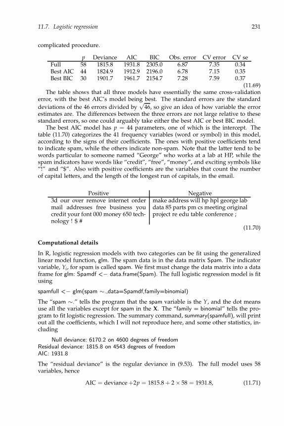
11.7. Logistic regression 231
complicated procedure.
p Deviance AIC BIC Obs. error CV error CV seFull 58 1815.8 1931.8 2305.0 6.87 7.35 0.34Best AIC 44 1824.9 1912.9 2196.0 6.78 7.15 0.35Best BIC 30 1901.7 1961.7 2154.7 7.28 7.59 0.37
(11.69)The table shows that all three models have essentially the same cross-validation
error, with the best AIC’s model being best. The standard errors are the standard
deviations of the 46 errors divided by√
46, so give an idea of how variable the errorestimates are. The differences between the three errors are not large relative to thesestandard errors, so one could arguably take either the best AIC or best BIC model.
The best AIC model has p = 44 parameters, one of which is the intercept. Thetable (11.70) categorizes the 41 frequency variables (word or symbol) in this model,according to the signs of their coefficients. The ones with positive coefficients tendto indicate spam, while the others indicate non-spam. Note that the latter tend to bewords particular to someone named “George” who works at a lab at HP, while thespam indicators have words like “credit”, “free”, “money”, and exciting symbols like“!” and “$”. Also with positive coefficients are the variables that count the numberof capital letters, and the length of the longest run of capitals, in the email.
Positive Negative3d our over remove internet ordermail addresses free business youcredit your font 000 money 650 tech-nology ! $ #
make address will hp hpl george labdata 85 parts pm cs meeting originalproject re edu table conference ;
(11.70)
Computational details
In R, logistic regression models with two categories can be fit using the generalizedlinear model function, glm. The spam data is in the data matrix Spam. The indicatorvariable, Yi, for spam is called spam. We first must change the data matrix into a dataframe for glm: Spamdf <− data.frame(Spam). The full logistic regression model is fitusing
spamfull <− glm(spam ∼.,data=Spamdf,family=binomial)
The “spam ∼.” tells the program that the spam variable is the Y, and the dot meansuse all the variables except for spam in the X. The “family = binomial” tells the pro-gram to fit logistic regression. The summary command, summary(spamfull), will printout all the coefficients, which I will not reproduce here, and some other statistics, in-cluding
Null deviance: 6170.2 on 4600 degrees of freedomResidual deviance: 1815.8 on 4543 degrees of freedomAIC: 1931.8
The “residual deviance” is the regular deviance in (9.53). The full model uses 58variables, hence
AIC = deviance+2p = 1815.8 + 2 × 58 = 1931.8, (11.71)
232 Chapter 11. Classification
which checks. The BIC is found by substituting log(4601) for the 2.We can find the predicted classifications from this fit using the function predict,
which returns the estimated linear Xβ from (11.67) for the fitted model. The Yi’s are
then 1 or 0 as the ρ(x(i) | c, a) is greater than or less than 1/2, i. e., as the Xβ is greateror less than 0. Thus to find the predictions and overall error rate, do
yhat <− ifelse(predict(spamfull)>0,1,0)sum(yhat!=Spamdf[,’spam’])/4601
We find the observed classification error to be 6.87%.
Cross-validation
We will use 46-fold cross-validation to estimate the classification error. We randomlydivide the 4601 observations into 46 groups of 100, leaving one observation whodoesn’t get to play. First, permute the indices from 1 to n:
o <− sample(1:4601)
Then the first hundred are the indices for the observations in the first leave-out-block,the second hundred in the second leave-out-block, etc. The loop is next, where theerr collects the number of classification errors in each block of 100.
err <− NULLfor(i in 1:46)
oi <− o[(1:100)+(i−1)∗100]yfiti <− glm(spam ∼., family = binomial,data = Spamdf,subset=(1:4601)[−oi])dhati <− predict(yfiti,newdata=Spamdf[oi,])yhati <− ifelse(dhati>0,1,0)err <− c(err,sum(yhati!=Spamdf[oi,’spam’]))
In the loop for cross-validation, the oi is the vector of indices being left out. We then fitthe model without those by using the keyword subset=(1:4601)[−oi], which indicatesusing all indices except those in oi. The dhati is then the vector of discriminantfunctions evaluated for the left out observations (the newdata). The mean of err is theestimated error, which for us is 7.35%. See the entry in table in (11.69).
Stepwise
The command to use for stepwise regression is step. To have the program searchthrough the entire set of variables, use one of the two statements
spamstepa <− step(spamfull,scope=list(upper= ∼.,lower = ∼1))spamstepb <− step(spamfull,scope=list(upper= ∼.,lower = ∼1),k=log(4601))
The first statement searches on AIC, the second on BIC. The first argument in the stepfunction is the return value of glm for the full data. The upper and lower inputs referto the formulas of the largest and smallest models one wishes to entertain. In ourcase, we wish the smallest model to have just the 1n vector (indicated by the “~1”),and the largest model to contain all the vectors (indicated by the “~.”).
These routines may take a while, and will spit out a lot of output. The end resultis the best model found using the given criterion. (If using the BIC version, whilecalculating the steps, the program will output the BIC values, though calling them

11.8. Trees 233
“AIC.” The summary output will give the AIC, calling it “AIC.” Thus if you use justthe summary output, you must calculate the BIC for yourself. )
To find the cross-validation estimate of classification error, we need to insert thestepwise procedure after fitting the model leaving out the observations, then predictthose left out using the result of the stepwise procedure. So for the best BIC model,use the following:
errb <− NULLfor(i in 1:46)
oi <− o[(1:100)+(i−1)∗100]yfiti <− glm(spam ∼., family = binomial, data = Spamdf,subset=(1:4601)[−oi])stepi <− step(yfiti,scope=list(upper= ∼.,lower = ∼1),k=log(4501))dhati <− predict(stepi,newdata=Spamdf[oi,])yhati <− ifelse(dhati>0,1,0)errb <− c(errb,sum(yhati!=Spamdf[oi,’spam’]))
The estimate for the best AIC model uses the same statements but with k = 2 inthe step function. This routine will take a while, because each stepwise procedureis time consuming. Thus one might consider using cross-validation on the modelchosen using the BIC (or AIC) criterion for the full data.
The neural networks R package nnet [Venables and Ripley, 2002] can be used to fitlogistic regression models for K > 2.
11.8 Trees
The presentation here will also use just K = 2 groups, labeled 0 and 1, but can beextended to any number of groups. In the logistic regression model (11.60), we mod-eled P[Y = 1 |X = x] ≡ ρ(x) using a particular parametric form. In this section weuse a simpler, nonparametric form, where ρ(x) is constant over rectangular regionsof the X-space.
To illustrate, we will use the South African heart disease data from Rossouw et al.[1983], which was used in Exercise 10.5.21. The Y is congestive heart disease (chd),where 1 indicates the person has the disease, 0 he does not. Explanatory variablesinclude various health measures. Hastie et al. [2009] apply logistic regression to thesedata. Here we use trees. Figure 11.5 plots the chd variable for the age and adiposity(fat percentage) variables. Consider the vertical line. It splits the data according towhether age is less than 31.5 years. The splitting point 31.5 was chosen so that theproportions of heart disease in each region would be very different. Here, 10/117 =8.85% of the men under age 31.5 had heart disease, while 150/345 = 43.48% of thoseabove 31.5 had the disease.
The next step is to consider just the men over age 31.5, and split them on theadiposity variable. Taking the value 25, we have that 41/106 = 38.68% of the menover age 31.5 but with adiposity under 25 have heart disease; 109/239 = 45.61% ofthe men over age 31.5 and with adiposity over 25 have the disease. We could furthersplit the younger men on adiposity, or split them on age again. Subsequent stepssplit the resulting rectangles, each time with either a vertical or horizontal segment.
There are also the other variables we could split on. It becomes easier to representthe splits using a tree diagram, as in Figure 11.6. There we have made several splits,at the nodes. Each node needs a variable and a cutoff point, such that people for

234 Chapter 11. Classification
20 30 40 50 60
1015
2025
3035
40
8.55%
45.61%
38.68%
Adi
posi
ty
Age
Figure 11.5: Splitting on age and adiposity. The open triangles indicate no heartdisease, the solid discs indicate heart disease. The percentages are the percentages ofmen with heart disease in each region of the plot.
which the variable is less than the cutoff are placed in the left branch, and the othersgo to the right. The ends of the branches are terminal nodes or leaves. This plot has 15leaves. At each leaf, there are a certain number of observations. The plot shows theproportion of 0’s (the top number) and 1’s (the bottom number) at each leaf.
For classification, we place a 0 or 1 at each leaf, depending on whether the pro-portion of 1’s is less than or greater than 1/2. Figure 11.7 shows the results. Notethat for some splits, both leaves have the same classification, because although theirproportions of 1’s are quite different, they are both on the same side of 1/2. For clas-sification purposes, we can snip some of the branches off. Further analysis (Section11.8.1) leads us to the even simpler tree in Figure 11.8. The tree is very easy to in-terpret, hence popular among people (e.g., doctors) who need to use them. The treealso makes sense, showing age, type A personality, tobacco use, and family historyare important factors in predicting heart disease among these men. The trees alsoare flexible, incorporating continuous and categorical variables, avoiding having toconsider transformations, and automatically incorporating interactions. E.g., the typeA variable shows up only for people between the ages of 31.5 and 50.5, and familyhistory and tobacco use show up only for people over 50.5.
Though simple to interpret, it is easy to imagine that finding the “best” tree is arather daunting prospect, as there is close to an infinite number of possible trees inany large data set (at each stage one can split any variable at any of a number ofpoints), and searching over all the possibilities is a very discrete (versus continuous)process. In the next section, we present a popular, and simple, algorithm to find a

11.8. Trees 235
|age < 31.5
tobacco < 0.51
alcohol < 11.105
age < 50.5
typea < 68.5 famhist:a
tobacco < 7.605
typea < 42.5
adiposity < 24.435
adiposity < 28.955
ldl < 6.705
tobacco < 4.15
adiposity < 28
typea < 48
0:1.001:0.01
1.000.00
0.600.40
0.700.30
0.200.80
1.000.00
0.900.08
0.600.40
0.001.00
0.500.50
0.600.40
0.001.00
0.700.30
0.200.80
0.051.00
Figure 11.6: A large tree, with proportions at the leaves.
good tree.
11.8.1 CART
Two popular commercial products for fitting trees are Categorization and Regression
Trees, CART®, by Breiman et al. [1984], and C5.0, an update of C4.5 by Quinlan[1993]. We will take the CART approach. Both approaches have R versions. It seemsthat CART would appeal more to statisticians, and C5.0 to data-miners, but I do notthink the results of the two methods would differ much.
We first need an objective function to measure the fit of a tree to the data. We willuse deviance, although other measures such as the observed misclassification rate arecertainly reasonable. For a tree T with L leaves, each observation is placed in one ofthe leaves. If observation yi is placed in leaf l, then that observation’s ρ(xi) is givenby the parameter for leaf l, say pl . The likelihood for that Bernoulli observation is
pyi
l (1 − pl)1−yi . (11.72)

236 Chapter 11. Classification
|age < 31.5
tobacco < 0.51
alcohol < 11.105
age < 50.5
typea < 68.5 famhist:a
tobacco < 7.605
typea < 42.5
adiposity < 24.435
adiposity < 28.955
ldl < 6.705
tobacco < 4.15
adiposity < 28
typea < 48
0
0 0
0 1
0
0 0
1 1
0 1
0
1
1
Figure 11.7: A large tree, with classifications at the leaves.
|age < 31.5
age < 50.5
typea < 68.5 famhist:a
tobacco < 7.605
0
0 1
0 1
1
Figure 11.8: A smaller tree, chosen using BIC.

11.8. Trees 237
Assuming the observations are independent, at leaf l there is a sample of iid Bernoullirandom variables with parameter pl , hence the overall likelihood of the sample is
L(p1, . . . , pL | y1, . . . , yn) =L
∏l=1
pwl
l (1 − pl)nl−wl , (11.73)
wherenl = #i at leaf l, wl = #yi = 1 at leaf l. (11.74)
This likelihood is maximized over the pl ’s by taking pl = wl/nl . Then the deviance(9.53) for this tree is
deviance(T ) = −2L
∑l=1
(wl log( pl) + (nl − wl) log(1 − pl)) . (11.75)
The CART method has two main steps: grow the tree, then prune the tree. Thetree is grown in a stepwise, greedy fashion, at each stage trying to find the nextsplit that maximally reduces the objective function. We start by finding the singlesplit (variable plus cutoff point) that minimizes the deviance among all such splits.Then the observations at each resulting leaf are optimally split, again finding thevariable/cutoff split with the lowest deviance. The process continues until the leaveshave just a few observations, e.g., stopping when any split would result in a leaf withfewer than five observations.
To grow the tree for the South African heart disease data in R, we need to installthe package called tree [Ripley, 2015]. A good explanation of it can be found inVenables and Ripley [2002]. We use the data frame SAheart in the ElemStatLearnpackage [Halvorsen, 2012]. The dependent variable is chd. To grow a tree, use
basetree <− tree(as.factor(chd)∼.,data=SAheart)
The as.factor function indicates to the tree function that it should do classification. Ifthe dependent variable is numeric, tree will fit a so-called regression tree, not whatwe want here. To plot the tree, use one of the two statements
plot(basetree);text(basetree,label=’yprob’,digits=1)plot(basetree);text(basetree)
The first gives the proportions of 0’s and 1’s at each leaf, and the second gives theclassifications of the leaves, yielding the trees in Figures 11.6 and 11.7, respectively.
This basetree is now our base tree, and we consider only subtrees, that is, treesobtainable by snipping branches off this tree. As usual, we would like to balanceobserved deviance with the number of parameters in the model, in order to avoidoverfitting. To whit, we add a penalty to the deviance depending on the number ofleaves in the tree. To use AIC or BIC, we need to count the number of parameters foreach subtree, conditioning on the structure of the base tree. That is, we assume thatthe nodes and the variable at each node are given, so that the only free parametersare the cutoff points and the pl ’s. The task is one of subset selection, that is, decidingwhich nodes to snip away. If the subtree has L leaves, then there are L − 1 cutoffpoints (there are L − 1 nodes), and L pl’s, yielding 2L − 1 parameters. Thus the BICcriterion for a subtree T with L leaves is
BIC(T ) = deviance(T ) + log(n)(2L − 1). (11.76)
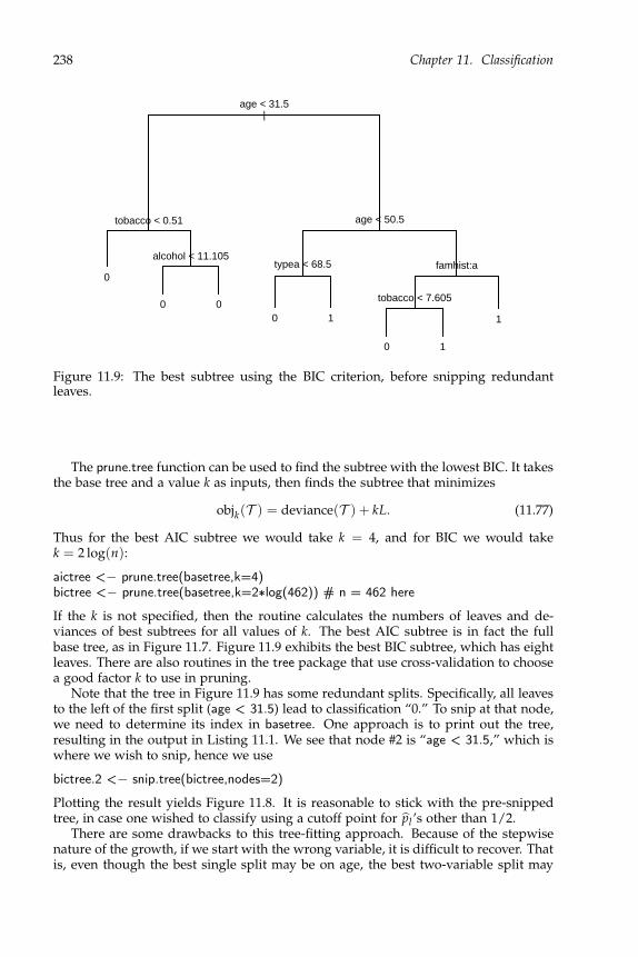
238 Chapter 11. Classification
|age < 31.5
tobacco < 0.51
alcohol < 11.105
age < 50.5
typea < 68.5 famhist:a
tobacco < 7.605
0
0 00 1
0 1
1
Figure 11.9: The best subtree using the BIC criterion, before snipping redundantleaves.
The prune.tree function can be used to find the subtree with the lowest BIC. It takesthe base tree and a value k as inputs, then finds the subtree that minimizes
objk(T ) = deviance(T ) + kL. (11.77)
Thus for the best AIC subtree we would take k = 4, and for BIC we would takek = 2 log(n):
aictree <− prune.tree(basetree,k=4)bictree <− prune.tree(basetree,k=2∗log(462)) # n = 462 here
If the k is not specified, then the routine calculates the numbers of leaves and de-viances of best subtrees for all values of k. The best AIC subtree is in fact the fullbase tree, as in Figure 11.7. Figure 11.9 exhibits the best BIC subtree, which has eightleaves. There are also routines in the tree package that use cross-validation to choosea good factor k to use in pruning.
Note that the tree in Figure 11.9 has some redundant splits. Specifically, all leavesto the left of the first split (age < 31.5) lead to classification “0.” To snip at that node,we need to determine its index in basetree. One approach is to print out the tree,resulting in the output in Listing 11.1. We see that node #2 is “age < 31.5,” which iswhere we wish to snip, hence we use
bictree.2 <− snip.tree(bictree,nodes=2)
Plotting the result yields Figure 11.8. It is reasonable to stick with the pre-snippedtree, in case one wished to classify using a cutoff point for pl ’s other than 1/2.
There are some drawbacks to this tree-fitting approach. Because of the stepwisenature of the growth, if we start with the wrong variable, it is difficult to recover. Thatis, even though the best single split may be on age, the best two-variable split may
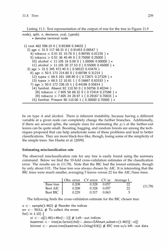
11.8. Trees 239
Listing 11.1: Text representation of the output of tree for the tree in Figure 11.9
node), split, n, deviance, yval, (yprob)∗ denotes terminal node
1) root 462 596.10 0 ( 0.65368 0.34632 )2) age < 31.5 117 68.31 0 ( 0.91453 0.08547 )
4) tobacco < 0.51 81 10.78 0 ( 0.98765 0.01235 ) ∗5) tobacco > 0.51 36 40.49 0 ( 0.75000 0.25000 )10) alcohol < 11.105 16 0.00 0 ( 1.00000 0.00000 ) ∗11) alcohol > 11.105 20 27.53 0 ( 0.55000 0.45000 ) ∗
3) age > 31.5 345 472.40 0 ( 0.56522 0.43478 )6) age < 50.5 173 214.80 0 ( 0.68786 0.31214 )12) typea < 68.5 161 188.90 0 ( 0.72671 0.27329 ) ∗13) typea > 68.5 12 10.81 1 ( 0.16667 0.83333 ) ∗
7) age > 50.5 172 236.10 1 ( 0.44186 0.55814 )14) famhist: Absent 82 110.50 0 ( 0.59756 0.40244 )
28) tobacco < 7.605 58 68.32 0 ( 0.72414 0.27586 ) ∗29) tobacco > 7.605 24 28.97 1 ( 0.29167 0.70833 ) ∗
15) famhist: Present 90 110.00 1 ( 0.30000 0.70000 ) ∗
be on type A and alcohol. There is inherent instability, because having a differentvariable at a given node can completely change the further branches. Additionally,if there are several splits, the sample sizes for estimating the pl ’s at the farther-outleaves can be quite small. Boosting, bagging, and random forests are among the tech-niques proposed that can help ameliorate some of these problems and lead to betterclassifications. They are more black-box-like, though, losing some of the simplicity ofthe simple trees. See Hastie et al. [2009].
Estimating misclassification rate
The observed misclassification rate for any tree is easily found using the summarycommand. Below we find the 10-fold cross-validation estimates of the classificationerror. The results are in (11.78). Note that the BIC had the lowest estimate, thoughby only about 0.01. The base tree was always chosen by AIC. It is interesting that theBIC trees were much smaller, averaging 5 leaves versus 22 for the AIC/base trees.
Obs. error CV error CV se Average LBase tree 0.208 0.328 0.057 22Best AIC 0.208 0.328 0.057 22Best BIC 0.229 0.317 0.063 5
(11.78)
The following finds the cross-validation estimate for the BIC chosen tree:
o <− sample(1:462) # Reorder the indiceserr <− NULL # To collect the errorsfor(i in 1:10)
oi <− o[(1:46)+46∗(i−1)] # Left−out indicesbasetreei <− tree(as.factor(chd)∼.,data=SAheart,subset=(1:462)[−oi])bictreei <− prune.tree(basetreei,k=2∗log(416)) # BIC tree w/o left−out data
240 Chapter 11. Classification
yhati <− predict(bictreei,newdata=SAheart[oi,],type=’class’)err <− c(err,sum(yhati!=SAheart[oi,’chd’]))
For each of the left-out observations, the predict statement with type=’class’ givesthe tree’s classification of the left-out observations. The estimate of the error is thenmean(err)/46, and the standard error is sd(err)/46.
11.9 Exercises
Exercise 11.9.1. Show that (11.19) follows from (11.18).
Exercise 11.9.2. Compare the statistic in (11.34) and its maximum using the a in
(11.35) to the motivation for Hotelling’s T2 presented in Section 8.4.1.
Exercise 11.9.3. Write the γk in (11.59) as a function of the θi’s and πi’s.
Exercise 11.9.4 (Spam). Consider the spam data from Section 11.7.2 and Exercise1.9.16. Here we simplify it a bit, and just look at four of the 0/1 predictors: Whetheror not the email contains the words “free” or “remove” or the symbols “!” or “$”.The following table summarizes the data, where the first four columns indicate thepresence (1) or absence (0) of the word or symbol, and the last two columns give thenumbers of corresponding emails that are spam or not spam. E.g., there are 98 emailscontaining “remove” and “!”, but not “free” nor “$”, 8 of which are not spam, 90 arespam.
free remove ! $ not spam spam0 0 0 0 1742 920 0 0 1 157 540 0 1 0 554 1610 0 1 1 51 2160 1 0 0 15 280 1 0 1 4 170 1 1 0 8 900 1 1 1 5 1661 0 0 0 94 421 0 0 1 28 201 0 1 0 81 1591 0 1 1 38 3051 1 0 0 1 161 1 0 1 0 331 1 1 0 2 1161 1 1 1 8 298
(11.79)
Assuming a multinomial distribution for the 25 = 32 possibilities, find the estimatedBayes classifier of email as “spam” or “not spam” based on the other four variablesin the table. What is the observed error rate?
Exercise 11.9.5 (Crabs). This problem uses data on 200 crabs, categorized into twospecies, orange and blue, and two sexes. It is in the MASS R package [Venablesand Ripley, 2002]. The data is in the data frame crabs. There are 50 crabs in eachspecies×sex category; the first 50 are blue males, then 50 blue females, then 50 orangemales, then 50 orange females. The five measurements are frontal lobe size, rear

11.9. Exercises 241
width, carapace length, carapace width, and body depth, all in millimeters. The goalhere is to find linear discrimination procedures for classifying new crabs into speciesand sex categories. (a) The basic model is that Y ∼ N(xβ, I200 ⊗ Σ), where x is anyanalysis of variance design matrix (n × 4) that distinguishes the four groups. Find the
MLE of Σ, Σ. (b) Find the ck’s and ak’s in Fisher’s linear discrimination for classifyingall four groups, i.e., classifying on species and sex simultaneously. (Take πk = 1/4 forall four groups.) Use the version wherein dK = 0. (c) Using the procedure in part (b)on the observed data, how many crabs had their species misclassified? How manyhad their sex misclassified? What was the overall observed misclassification rate (forsimultaneous classification of color and sex)? (d) Use leave-one-out cross-validationto estimate the overall misclassification rate. What do you get? Is it higher than theobserved rate in part (c)?
Exercise 11.9.6 (Crabs). Continue with the crabs data from Exercise 11.9.5, but useclassification trees to classify the crabs by just species. (a) Find the base tree using thecommand
crabtree <− tree(sp ∼FL+RW+CL+CW+BD,data=crabs)
How many leaves does the tree have? Snip off redundant nodes. How many leavesdoes the snipped tree have? What is its observed misclassification rate? (b) Find theBIC for the subtrees found using prune.tree. Give the number of leaves, deviance,and dimension for the subtree with the best BIC. (c) Consider the subtree with thebest BIC. What is its observed misclassification rate? What two variables figure mostprominently in the tree? Which variables do not appear? (d) Now find the leave-one-out cross-validation estimate of the misclassification error rate for the best modelusing BIC. How does this rate compare with the observed rate?
Exercise 11.9.7 (South African heart disease). This question uses the South Africanheart disease study discussed in Section 11.8. The objective is to use logistic regres-sion to classify people on the presence of heart disease, variable chd. (a) Use thelogistic model that includes all the explanatory variables to do the classification. (b)Find the best logistic model using the stepwise function, with BIC as the criterion.Which variables are included in the best model from the stepwise procedure? (c) Usethe model with just the variables suggested by the factor analysis of Exercise 10.5.21:tobacco, ldl, adiposity, obesity, and alcohol. (d) Find the BIC, observed error rate, andleave-one-out cross-validation rate for the three models in parts (a), (b) and (c). (e)True or false: (i) The full model has the lowest observed error rate; (ii) The factor-analysis-based model is generally best; (iii) The cross-validation-based error rates aresomewhat larger than the corresponding observed error rates; (iv) The model withthe best observed error rate has the best cross-validation-based error rate as well; (v)The best model of these three is the one chosen by the stepwise procedure; (vi) Bothadiposity and obesity seem to be important factors in classifying heart disease.
Exercise 11.9.8 (Zipcode). The objective here is to classify handwritten numerals(0, 1, . . . , 9), so that machines can read people’s handwritten zipcodes. The data setconsists of 16 × 16 grayscale images, that is, each numeral has been translated to a16 × 16 matrix, where the elements of the matrix indicate the darkness (from −1 to1) of the image at 256 grid points. The data set is from LeCun [1989], and can befound in the R package StatElemLearn [Halvorsen, 2012]. This question will use justthe 7’s, 8’s and 9’s, for which there are n = 1831 observations. We put the data inthree matrices, one for each digit, called train7, train8, and train9. Each row contains

242 Chapter 11. Classification
first the relevant digit, then the 256 grayscale values, for one image. The task is to uselinear discrimination to distinguish between the digits, even though it is clear thatthe data are not multivariate normal. First, create the three matrices from the largezip.train matrix:
train7 <− zip.train[zip.train[,1]==7,−1]train8 <− zip.train[zip.train[,1]==8,−1]train9 <− zip.train[zip.train[,1]==9,−1]
(a) Using the image, contour, and matrix functions in R, reconstruct the images ofsome of the 7’s, 8’s and 9’s from their grayscale values. (Or explore the zip2imagefunction in the StatElemLearn package.) (b) Use linear discrimination to classify theobservations based on the 256 variables under the three scenarios below. In each case,find both the observed misclassification rate and the estimate using cross-validation.(i) Using Σ = I256. (ii) Assuming Σ is diagonal, using the pooled estimates of theindividual variances. (iii) Using the pooled covariance matrix as an estimate of Σ.(d) Which method had the best error rate, estimated by cross-validation? (e) Create adata set of digits (7’s, 8’s, and 9’, as well as 5’s) to test classifiers as follows:
test5 <− zip.test[zip.test[,1]==5,−1]test7 <− zip.test[zip.test[,1]==7,−1]test8 <− zip.test[zip.test[,1]==8,−1]test9 <− zip.test[zip.test[,1]==9,−1]
Using the discriminant functions from the original data for the best method from part(b), classify these new observations. What is the error rate for the 7’s, 8’s, and 9’s?How does it compare with the cross-validation estimate? How are the 5’s classified?
Exercise 11.9.9 (Spam). Use classification trees to classify the spam data. It is best tostart as follows:
Spamdf <− data.frame(Spam)spamtree <− tree(as.factor(spam)∼.,data=Spamdf)
Turning the matrix into a data frame makes the labeling on the plots simpler. (a)Find the BIC’s for the subtrees obtained using prune.tree. How many leaves are inthe best model? What is its BIC? What is its observed error rate? (b) Use 46-foldcross-validation (so you leave out 100 observations each time) to estimate the errorrate, as in the procedure on page 239. (c) Repeat parts (a) and (b), but using thefirst ten principal components of the spam explanatory variables as the predictors.(Exercise 1.9.17 calculated the principal components.) Repeat again, but this timeusing the first ten principal components based on the scaled explanatory variables,scale(Spam[,1:57]). Compare the effectiveness of the three approaches.
Exercise 11.9.10. This question develops a Bayes classifier when there is a mix of nor-mal and binomial explanatory variables. Consider the classification problem basedon (Y, X, Z), where Y is the variable to be classified, with values 0 and 1, and X andZ are predictors. X is a 1 × 2 continuous vector, and Z takes the values 0 and 1. Themodel for (Y, X, Z) is given by
X |Y = y, Z = z ∼ N(µyz, Σ), (11.80)
and
P[Y = y & Z = z] = pyz, (11.81)

11.9. Exercises 243
so that p00 + p01 + p10 + p11 = 1. (a) Find an expression for P[Y = y |X = x & Z =z]. (b) Find the 1 × 2 vector αz and the constant γz (which depend on z and theparameters) so that
P[Y = 1 | X = x & Z = z] > P[Y = 0 | X = x & Z = z] ⇔ xα′z + γz > 0. (11.82)
(c) Suppose the data are (Yi, Xi, Zi), i = 1, . . . , n, iid, distributed as above. Findexpressions for the MLE’s of the parameters (the four µyz’s, the four pyz’s, and Σ).
Exercise 11.9.11 (South African heart disease). Apply the classification method in Ex-ercise 11.9.10 to the South African heart disease data, with Y indicating heart disease(chd), X containing the two variables age and type A, and Z being the family historyof heart disease variable (history: 0 = absent, 1 = present). Randomly divide the datainto two parts: The training data with n = 362, and the test data with n = 100. E.g.,use
random.index <− sample(462,100)sahd.train <− SAheart[−random.index,]sahd.test <− SAheart[random.index,]
(a) Estimate the αz and γz using the training data. Find the observed misclassification
rate on the training data, where you classify an observation as Yi = 1 if xiαz + γz > 0,
and Yi = 0 otherwise. What is the misclassification rate for the test data (using theestimates from the training data)? Give the 2 × 2 table showing true and predictedY’s for the test data. (b) Using the same training data, find the classification tree. Youdon’t have to do any pruning. Just take the full tree from the tree program. Find themisclassification rates for the training data and the test data. Give the table showingtrue and predicted Y’s for the test data. (c) Still using the training data, find theclassification using logistic regression, with the X and Z as the explanatory variables.What are the coefficients for the explanatory variables? Find the misclassificationrates for the training data and the test data. (d) What do you conclude?

Chapter 12
Clustering
The classification and prediction we have covered in previous chapters were casesof supervised learning. For example, in classification, we try to find a function thatclassifies individuals into groups using their X values, where in the training set weknow what the proper groups are because we observe their Y’s. In clustering, weagain wish to classify observations into groups using their X’s, but do not know thecorrect groups even in the training set, i.e., we do not observe the Y’s, nor often evenknow how many groups there are. Clustering is a case of unsupervised learning.
There are many clustering algorithms. In this chapter we focus on a few of them.Most are reasonably easy to implement given the number K of clusters. The diffi-cult part is deciding what K should be. Unlike in classification, there is no obviouscross-validation procedure to balance the number of clusters with the tightness of theclusters. Only in the model-based clustering do we have direct AIC or BIC criteria.Otherwise, a number of reasonable but ad hoc measures have been proposed. We willlook at “silhouettes.”
In some situations one is not necessarily assuming that there are underlying clus-ters, but rather is trying to divide the observations into a certain number of groupsfor other purposes. For example, a teacher in a class of 40 students might want tobreak up the class into four sections of about ten each based on general ability (togive more focused instruction to each group). The teacher does not necessarily thinkthere will be wide gaps between the groups, but still wishes to divide for pedagogicalpurposes. In such cases K is fixed, so the task is a bit simpler.
In general, though, when clustering one is looking for groups that are well sep-arated. There is often an underlying model, just as in Chapter 11 on model-basedclassification. That is, the data are
(X1, Y1), . . . , (Xn, Yn), iid, (12.1)
where Yi ∈ 1, . . . , K,
X |Y = k ∼ fk(x) = f (x | θk) and P[Y = k] = πk, (12.2)
as in (11.2) and (11.3). If the parameters are known, then the clustering proceedsexactly as for classification, where an observation x is placed into the group
C(x) = k that maximizesfk(x)πk
f1(x)π1 + · · ·+ fK(x)πK. (12.3)
245

246 Chapter 12. Clustering
See (11.13). The fly in the ointment is that we do not observe the yi’s (neither in thetraining set nor for the new observations), nor do we necessarily know what K is, letalone the parameter values.
The following sections look at some approaches to clustering. The first, K-means,
does not explicitly use a model, but has in the back of its mind fk’s being N(µk, σ2Ip).Hierarchical clustering avoids the problems of number of clusters by creating a treecontaining clusterings of all sizes, from K = 1 to n. Finally, the model-based cluster-ing explicitly assumes the fk’s are multivariate normal (or some other given distribu-tion), with various possibilities for the covariance matrices.
12.1 K-means
For a given number K of groups, K-means assumes that each group has a mean vectorµk. Observation xi is assigned to the group with the closest mean. To estimate thesemeans, we minimize the sum of the squared distances from the observations to theirgroup means:
obj(µ1, . . . ,µK) =n
∑i=1
minµ1,...,µK
‖xi −µk‖2. (12.4)
An algorithm for finding the clusters starts with a random set of means µ1, . . . , µK
(e.g., randomly choose K observations from the data), then iterate the following twosteps:
1. Having estimates of the means, assign observations to the group correspondingto the closest mean,
C(xi) = k that minimizes ‖xi − µk‖2 over k. (12.5)
2. Having individuals assigned to groups, find the group means,
µk =1
#C(xi) = k ∑i|C(xi)=k
xi . (12.6)
The algorithm is guaranteed to converge (if ties among the closest means are han-dled properly), but not necessarily to the global minimum. It is a good idea to tryseveral random starts, then take the one that yields the lowest obj in (12.4). Theresulting means and assignments are the K-means and their clustering.
12.1.1 Example: Sports data
Recall the data on people ranking seven sports presented in Section 1.6.2. Using theK-means algorithm for K = 1, . . . , 4, we find the following means (where K = 1 givesthe overall mean):

12.1. K-means 247
K = 1 BaseB FootB BsktB Ten Cyc Swim JogGroup 1 3.79 4.29 3.74 3.86 3.59 3.78 4.95
K = 2 BaseB FootB BsktB Ten Cyc Swim JogGroup 1 5.01 5.84 4.35 3.63 2.57 2.47 4.12Group 2 2.45 2.60 3.06 4.11 4.71 5.21 5.85
K = 3 BaseB FootB BsktB Ten Cyc Swim JogGroup 1 2.33 2.53 3.05 4.14 4.76 5.33 5.86Group 2 4.94 5.97 5.00 3.71 2.90 3.35 2.13Group 3 5.00 5.51 3.76 3.59 2.46 1.90 5.78
K = 4 BaseB FootB BsktB Ten Cyc Swim JogGroup 1 5.10 5.47 3.75 3.60 2.40 1.90 5.78Group 2 2.30 2.10 2.65 5.17 4.75 5.35 5.67Group 3 2.40 3.75 3.90 1.85 4.85 5.20 6.05Group 4 4.97 6.00 5.07 3.80 2.80 3.23 2.13
(12.7)
Look at the K = 2 means. Group 1 likes swimming and cycling, while group 2likes the team sports, baseball, football, and basketball. If we compare these to theK = 3 clustering, we see group 1 appears to be about the same as the team sportsgroup from K = 2, while groups 2 and 3 both like swimming and cycling. Thedifference is that group 3 does not like jogging, while group 2 does. For K = 4, itlooks like the team-sports group has split into one that likes tennis (group 3), andone that doesn’t (group 2). At this point it may be more useful to try to decidewhat number of clusters is “good.” (Being able to interpret the clusters is one goodcharacteristic.)
12.1.2 Silhouettes
One measure of clustering efficacy is Rousseeuw’s [1987] notion of silhouettes. Thesilhouette of an observation i measures how well it fits in its own cluster versus howwell it fits in its next closest cluster. For K-means, we have changed the originaldefinition a little. Let
a(i) = ‖xi − µk‖2 and b(i) = ‖xi − µl‖2, (12.8)
where observation i is assigned to group k, and group l has the next-closest groupmean to xi. Then its silhouette is
silhouette(i) =b(i)− a(i)
maxa(i), b(i) . (12.9)
By construction, b(i) ≥ a(i), hence the denominator is b(i), and the silhouette takesvalues between 0 and 1. If the observation is equal to its group mean, its silhouetteis 1. If it is halfway between the two group means, its silhouette is 0. For otherclusterings (K-medoids, as in Section 12.2, for example), the silhouettes can rangefrom -1 to 1, but usually stay above 0, or at least do not go much below.
Figure 12.1 contains the silhouettes for K’s from 2 to 5 for the sports data. Theobservations (along the horizontal axis) are arranged by group and, within group,
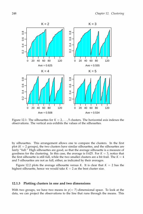
248 Chapter 12. Clustering
0 20 40 60 80 120
0.2
0.4
0.6
0.8
Ave = 0.625
K = 2
0 20 40 60 80 120
0.2
0.4
0.6
0.8
Ave = 0.555
K = 3
0 20 40 60 80 120
0.2
0.4
0.6
0.8
Ave = 0.508
K = 4
0 20 40 60 80 120
0.2
0.4
0.6
0.8
Ave = 0.534
K = 5
Figure 12.1: The silhouettes for K = 2, . . . , 5 clusters. The horizontal axis indexes theobservations. The vertical axis exhibits the values of the silhouettes.
by silhouettes. This arrangement allows one to compare the clusters. In the firstplot (K = 2 groups), the two clusters have similar silhouettes, and the silhouettes arefairly “full.” High silhouettes are good, so that the average silhouette is a measure ofgoodness for the clustering. In this case, the average is 0.625. For K = 3, notice thatthe first silhouette is still full, while the two smaller clusters are a bit frail. The K = 4and 5 silhouettes are not as full, either, as indicated by their averages.
Figure 12.2 plots the average silhouette versus K. It is clear that K = 2 has thehighest silhouette, hence we would take K = 2 as the best cluster size.
12.1.3 Plotting clusters in one and two dimensions
With two groups, we have two means in p(= 7)-dimensional space. To look at thedata, we can project the observations to the line that runs through the means. This

12.1. K-means 249
2 4 6 8 10
0.52
0.56
0.60
K
Figure 12.2: The average silhouettes for K = 2, . . . , 10 clusters.
projection is where the clustering is taking place. Let
z =µ1 − µ2
‖µ1 − µ2‖, (12.10)
the unit vector pointing from µ2 to µ1. Then using z as an axis, the projections of theobservations onto z have coordinates
wi = xiz′, i = 1, . . . , N. (12.11)
Figure 12.3 is the histogram for the wi’s, where group 1 has wi > 0 and group 2 haswi < 0. We can see that the clusters are well-defined in that the bulk of each clusteris far from the center of the other cluster.
We have also plotted the sports, found by creating a “pure” ranking for each sport.Thus the pure ranking for baseball would give baseball the rank of 1, and the othersports the rank of 4.5, so that the sum of the ranks, 28, is the same as for the otherrankings. Adding these sports to the plot helps aid in interpreting the groups: teamsports on the left, individual sports on the right, with tennis on the individual-sportside, but close to the border.
If K = 3, then the three means lie in a plane, hence we would like to project theobservations onto that plane. One approach is to use principal components (Section1.6) on the means. Because there are three, only the first two principal componentswill have positive variance, so that all the action will be in the first two. Letting
Z =
µ1µ2µ3
, (12.12)
we apply the spectral decomposition (1.33) in Theorem 1.1 to the sample covariancematrix of Z:
1
3Z′H3Z = GLG′, (12.13)

250 Chapter 12. Clustering
−6 −4 −2 0 2 4 6
02
46
810
W
−6 −4 −2 0 2 4 6
02
46
810 Baseball
FootballBasketball
TennisCyclingSwimming
Jogging
Figure 12.3: The histogram for the observations along the line connecting the twomeans for K = 2 groups.
where G is orthogonal and L is diagonal. The diagonals of L here are 11.77, 4.07, andfive zeros. We then rotate the data and the means using G,
W = XG and W(means) = ZG. (12.14)
Figure 12.4 plots the first two variables for W and W(means), along with the sevenpure rankings. We see the people who like team sports to the right, and the peoplewho like individual sports to the left, divided into those who can and those whocannot abide jogging. Compare this plot to the biplot that appears in Figure 1.6.
12.1.4 Example: Sports data, using R
The sports data is in the R matrix sportsranks. The K-means clustering uses the func-tion kmeans. This routine uses the method in Hartigan and Wong [1979], whichtweaks the basic algorithm in (12.5) and (12.6) by some intelligent reassigning of
individual points. We create a list whose Kth component contains the results forK = 2, . . . , 10 groups:
kms <− vector(’list’,10)for(K in 2:10)
kms[[K]] <− kmeans(sportsranks,centers=K,nstart=10)
The centers input specifies the number of groups desired, and nstart=10 means ran-domly start the algorithm ten times, then use the one with lowest within sum ofsquares. The output in kms[[K]] for the K-group clustering is a list with centers, theK × p of estimated cluster means; cluster, an n-vector that assigns each observationto its cluster (i.e., the yi’s); withinss, the K-vector of SSk’s (so that SS(K) is found

12.1. K-means 251
−4 −2 0 2 4
−2
02
4
Var 1
Var
2
1
2
3
BaseballFootball
Basketball
Tennis
Cycling
Swimming
Jogging
Figure 12.4: The scatter plot for the data projected onto the plane containing themeans for K = 3.
by sum(kms[[K]]$withinss)); and size, the K-vector giving the numbers of observationsassigned to each group.
Silhouettes
Section A.4.1 contains a simple function for calculating the silhouettes in (12.9) fora given K-means clustering. The sort_silhouette function in Section A.4.2 sorts thesilhouette values for plotting. The following statements produce Figure 12.1:
sil.ave <− NULL # To collect silhouette’s means for each Kpar(mfrow=c(3,3))for(K in 2:10)
sil <− silhouette.km(sportsranks,kms[[K]]$centers)sil.ave <− c(sil.ave,mean(sil))ssil <− sort_silhouette(sil,kms[[K]]$cluster)plot(ssil,type=’h’,xlab=’Observations’,ylab=’Silhouettes’)title(paste(’K =’,K))

252 Chapter 12. Clustering
The sil.ave calculated above can then be used to obtain Figure 12.2:
plot(2:10,sil.ave,type=’l’,xlab=’K’,ylab=’Average silhouette width’)
Plotting the clusters
Finally, we make plots as in Figures 12.3 and 12.4. For K = 2, we have the one z as in(12.10) and the wi’s as in (12.11):
z <− kms[[2]]$centers[1,]−kms[[2]]$centers[2,]z <− z/sqrt(sum(z^2))w <− sportsranks%∗%zxl <− c(−6,6); yl <− c(0,13) # Fix the x− and y−rangeshist(w[kms[[2]]$cluster==1],col=2,xlim=xl,ylim=yl,main=’K=2’,xlab=’W’)par(new=TRUE) # To allow two histograms on the same plothist(w[kms[[2]]$cluster==2],col=3,xlim=xl,ylim=yl,main=’ ’,xlab=’ ’)
To add the sports’ names:
y <− matrix(4.5,7,7)−3.5∗diag(7)ws <− y%∗%ztext(ws,c(10,11,12,8,9,10,11),labels=dimnames(sportsranks)[[2]])
The various placement numbers were found by trial and error.For K = 3, or higher, we can use R’s eigenvector/eigenvalue function, eigen, to
find the G used in (12.14):
z <− kms[[3]]$centersg <− eigen(var(z))$vectors[,1:2] # Just need the first two columnsw <− sportsranks%∗%g # For the observationsws <− y%∗%g # For the sports’ nameswm <− z%∗%g # For the groups’ meanscl <− kms[[3]]$clusterplot(w,xlab=’Var 1’,ylab=’Var 2’,pch=cl)text(wc,labels=1:3)text(ws,dimnames(sportsranks)[[2]])
12.2 K-medoids
Clustering with medoids [Kaufman and Rousseeuw, 1990] works directly on dis-tances between objects. Suppose we have n objects, o1, . . . , on, and a dissimilaritymeasure d(oi, oj) between pairs. This d satisfies
d(oi, oj) ≥ 0, d(oi, oj) = d(oj, oi), and d(oi, oi) = 0, (12.15)
but it may not be an actual metric in that it need not satisfy the triangle inequality.Note that one cannot necessarily impute distances between an object and anothervector, e.g., a mean vector. Rather than clustering around means, the clusters are thenbuilt around some of the objects. That is, K-medoids finds K of the objects (c1, . . . , cK)to act as centers (or medoids), the objective being to find the set that minimizes
obj(c1, . . . , cK) =N
∑i=1
minc1,...,cK
d(oi, ck). (12.16)

12.2. K-medoids 253
Each object is then assigned to the group corresponding to the closest of the ck’s.Silhouettes are defined as in (12.9), except that here, for each observation i,
a(i) =1
# Group k ∑j ∈ Group k
d(oi, oj) and b(i) =1
# Group l ∑j ∈ Group l
d(oi, oj),
(12.17)where group k is object i’s group, and group l is its next closest group.
In R, one can use the package cluster [Maechler et al., 2015], which implementsK-medoids clustering in the function pam, which stands for partitioning aroundmedoids. Consider the grades data in Section 4.2.1. We will cluster the five vari-ables, homework, labs, inclass, midterms, and final, not the 107 people. A naturalmeasure of similarity between two variables is their correlation. Instead of using theusual Pearson coefficient, we will use Kendall’s τ, which is more robust. For n × 1vectors x and y, Kendall’s τ is
T(x, y) =∑1≤i<j≤n Sign(xi − xj)Sign(yi − yj)
(n2)
. (12.18)
The numerator looks at the line segment connecting each pair of points (xi, yi) and(xj, yj), counting +1 if the slope is positive and −1 if it is negative. The denominator
normalizes the statistic so that it is between ±1. Then T(x, y) = +1 means that thexi’s and yi’s are exactly monotonically increasingly related, and −1 means they areexactly monotonically decreasingly related, much as the correlation coefficient. TheT’s measure similarities, so we subtract each T from 1 to obtain the dissimilaritymatrix:
HW Labs InClass Midterms FinalHW 0.00 0.56 0.86 0.71 0.69Labs 0.56 0.00 0.80 0.68 0.71InClass 0.86 0.80 0.00 0.81 0.81Midterms 0.71 0.68 0.81 0.00 0.53Final 0.69 0.71 0.81 0.53 0.00
(12.19)
Using R, we find the dissimilarity matrix:
x <− grades[,2:6]dx <− matrix(nrow=5,ncol=5) # To hold the dissimilaritiesfor(i in 1:5)
for(j in 1:5)dx[i,j] <− 1−cor.test(x[,i],x[,j],method=’kendall’)$est
This matrix is passed to the pam function, along with the desired number of groupsK. Thus for K = 3, say, use
pam3 <− pam(as.dist(dx),k=3)
The average silhouette for this clustering is in pam3$silinfo$avg.width. The results forK = 2, 3 and 4 are
K 2 3 4Average silhouette 0.108 0.174 0.088
(12.20)
We see that K = 3 has the best average silhouette. The assigned groups for this clus-tering can be found in pam3$clustering, which is (1,1,2,3,3), meaning the groupings
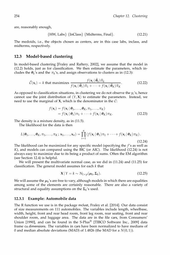
254 Chapter 12. Clustering
are, reasonably enough,
HW, Labs InClass Midterms, Final. (12.21)
The medoids, i.e., the objects chosen as centers, are in this case labs, inclass, andmidterms, respectively.
12.3 Model-based clustering
In model-based clustering [Fraley and Raftery, 2002], we assume that the model in(12.2) holds, just as for classification. We then estimate the parameters, which in-cludes the θk’s and the πk’s, and assign observations to clusters as in (12.3):
C(xi) = k that maximizesf (xi | θk)πk
f (xi | θ1)π1 + · · ·+ f (xi | θK)πK
. (12.22)
As opposed to classification situations, in clustering we do not observe the yi’s, hencecannot use the joint distribution of (Y, X) to estimate the parameters. Instead, weneed to use the marginal of X, which is the denominator in the C:
f (xi) = f (xi | θ1, . . . , θK, π1, . . . , πK)
= f (xi | θ1)π1 + · · ·+ f (xi | θK)πK. (12.23)
The density is a mixture density, as in (11.5).The likelihood for the data is then
L(θ1, . . . ,θK , π1, . . . , πK ; x1, . . . , xn) =n
∏i=1
( f (xi | θ1)π1 + · · ·+ f (xi | θK)πK) .
(12.24)The likelihood can be maximized for any specific model (specifying the f ’s as well asK), and models can compared using the BIC (or AIC). The likelihood (12.24) is notalways easy to maximize due to its being a product of sums. Often the EM algorithm(see Section 12.4) is helpful.
We will present the multivariate normal case, as we did in (11.24) and (11.25) forclassification. The general model assumes for each k that
X |Y = k ∼ N1×p(µk, Σk). (12.25)
We will assume the µk’s are free to vary, although models in which there are equalitiesamong some of the elements are certainly reasonable. There are also a variety ofstructural and equality assumptions on the Σk’s used.
12.3.1 Example: Automobile data
The R function we use is in the package mclust, Fraley et al. [2014]. Our data consistof size measurements on 111 automobiles. The variables include length, wheelbase,width, height, front and rear head room, front leg room, rear seating, front and rearshoulder room, and luggage area. The data are in the file cars, from Consumers’
Union [1990], and can be found in the S-Plus® [TIBCO Software Inc., 2009] dataframe cu.dimensions. The variables in cars have been normalized to have medians of0 and median absolute deviations (MAD) of 1.4826 (the MAD for a N(0, 1)).

12.3. Model-based clustering 255
2 4 6 8
−60
00−
5000
−40
00
EIIVIIEEIVEIEVI
VVIEEEEEVVEVVVV
K
−B
IC
Figure 12.5: −BIC’s for fitting the entire data set.
The routine we’ll use is Mclust (be sure to capitalize the M). It will try variousforms of the covariance matrices and group sizes, and pick the best based on the BIC.To use the default options and have the results placed in mcars, use
mcars <− Mclust(cars)
There are many options for plotting in the package. To see a plot of the BIC’s, use
plot(mcars,cars,what=’BIC’)
You have to click on the graphics window, or hit enter, to reveal the plot. The resultis in Figure 12.5. The horizontal axis specifies the K, and the vertical axis gives theBIC values, although these are the negatives of our BIC’s. The symbols plotted onthe graph are codes for various structural hypotheses on the covariances. See (12.31).In this example, the best model is Model “VVV” with K = 2, which means thecovariance matrices are arbitrary and unequal.
Some pairwise plots (length versus height, width versus front head room, andrear head room versus luggage) are given in Figure 12.6. The plots include ellipses toillustrate the covariance matrices. Indeed we see that the two ellipses in each plot arearbitrary and unequal. To plot variable 1 (length) versus variable 4 (height), use
plot(mcars,cars,what=’classification’,dimens=c(1,4))
We also plot the first two principal components (Section 1.6). The matrix of eigenvec-tors, G in (1.33), is given by eigen(var(cars))$vectors:
carspc <− cars%∗%eigen(var(cars))$vectors # Principal components

256 Chapter 12. Clustering
−4 −2 0 2 4
−5
05
1015
20
Length
Hei
ght
−4 −2 0 2 4
−4
−2
02
4
Width
Fro
nt h
ead
room
−4 −2 0 2 4 6
−8
−4
02
4
Rear head room
Lugg
age
0 10 20 30
−20
−10
05
PC1
PC
2
Figure 12.6: Some two-variable plots of the clustering produced by Mclust. The solidtriangles indicate group 1, and the open squares indicate group 2. The fourth graphplots the first two principal components of the data.
To obtain the ellipses, we redid the clustering using the principal components as thedata, and specifying G=2 groups in Mclust.
Look at the plots. The lower left graph shows that group 2 is almost constanton the luggage variable. In addition, the upper left and lower right graphs indicatethat group 2 can be divided into two groups, although the BIC did not pick up thedifference. The Table 12.1 exhibits four of the variables for the 15 automobiles ingroup 2.
We have divided this group as suggested by the principal component plot. Notethat the first group of five are all sports cars. They have no back seats or luggage areas,hence the values in the data set for the corresponding variables are coded somehow.The other ten automobiles are minivans. They do not have specific luggage areas, i.e.,trunks, either, although in a sense the whole vehicle is a big luggage area. Thus thisgroup really is a union of two smaller groups, both of which are quite a bit differentthan group 1.
We now redo the analysis on just the group 1 automobiles:
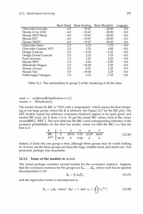
12.3. Model-based clustering 257
Rear Head Rear Seating Rear Shoulder LuggageChevrolet Corvette −4.0 −19.67 −28.00 −8.0Honda Civic CRX −4.0 −19.67 −28.00 −8.0Mazda MX5 Miata −4.0 −19.67 −28.00 −8.0Mazda RX7 −4.0 −19.67 −28.00 −8.0Nissan 300ZX −4.0 −19.67 −28.00 −8.0Chevrolet Astro 2.5 0.33 −1.75 −8.0Chevrolet Lumina APV 2.0 3.33 4.00 −8.0Dodge Caravan 2.5 −0.33 −6.25 −8.0Dodge Grand Caravan 2.0 2.33 3.25 −8.0Ford Aerostar 1.5 1.67 4.25 −8.0Mazda MPV 3.5 0.00 −5.50 −8.0Mitsubishi Wagon 2.5 −19.00 2.50 −8.0Nissan Axxess 2.5 0.67 1.25 −8.5Nissan Van 3.0 −19.00 2.25 −8.0Volkswagen Vanagon 7.0 6.33 −7.25 −8.0
Table 12.1: The automobiles in group 2 of the clustering of all the data.
cars1 <− cars[mcars$classification==1,]mcars1 <− Mclust(cars1)
The model chosen by BIC is “XXX with 1 components” which means the best cluster-ing is one large group, where the Σ is arbitrary. See Figure 12.7 for the BIC plot. TheEEE models (equal but arbitrary covariance matrices) appear to be quite good, andsimilar BIC-wise, for K from 1 to 4. To get the actual BIC values, look at the vectormcars1$BIC[,’’EEE’’]. The next table has the BIC’s and corresponding estimates of theposterior probabilities for the first five model, where we shift the BIC’s so that thebest is 0:
K 1 2 3 4 5BIC 0 28.54 9.53 22.09 44.81
PBIC 99.15 0 0.84 0 0(12.26)
Indeed, it looks like one group is best, although three groups may be worth lookingat. It turns out the three groups are basically large, middle-sized, and small cars. Notprofound, perhaps, but reasonable.
12.3.2 Some of the models in mclust
The mclust package considers several models for the covariance matrices. Supposethat the covariance matrices for the groups are Σ1, . . . , ΣK, where each has its spectraldecomposition (1.33)
Σk = ΓkΛkΓ′k, (12.27)
and the eigenvalue matrix is decomposed as
Λk = ck∆k where |∆k| = 1 and ck = [p
∏j=1
λj]1/p, (12.28)

258 Chapter 12. Clustering
2 4 6 8
−42
00−
3800
−34
00−
3000
EIIVIIEEIVEIEVI
VVIEEEEEVVEVVVV
K
−B
IC
Figure 12.7: −BIC’s for the data set without the sports cars or minivans.
the geometric mean of the eigenvalues. A covariance matrix is then described byshape, volume, and orientation:
Shape(Σk) = ∆k;
Volume(Σk) = |Σk| = cpk ;
Orientation(Σk) = Γk. (12.29)
The covariance matrices are then classified into spherical, diagonal, and ellipsoidal:
Spherical ⇒ ∆k = Ip ⇒ Σk = ckIp;
Diagonal ⇒ Γk = Ip ⇒ Σk = ckDk;
Ellipsoidal ⇒ Σk is arbitrary. (12.30)
The various models are defined by the type of covariances, and what equalitiesthere are among them. I haven’t been able to crack the code totally, but the descrip-tions tell the story. When K ≥ 2 and p ≥ 2, the following table may help translate thedescriptions into restrictions on the covariance matrices through (12.29) and(12.30):

12.4. The EM algorithm 259
Code Description Σk
EII spherical, equal volume σ2Ip
VII spherical, unequal volume σ2k Ip
EEI diagonal, equal volume and shape Λ
VEI diagonal, varying volume, equal shape ck∆
EVI diagonal, equal volume, varying shape c∆kVVI diagonal, varying volume and shape ΛkEEE ellipsoidal, equal volume, shape, and orientation Σ
EEV ellipsoidal, equal volume and equal shape ΓkΛΓ′k
VEV ellipsoidal, equal shape ckΓk∆Γ′k
VVV ellipsoidal, varying volume, shape, and orientation arbitrary
(12.31)
Here, Λ’s are diagonal matrices with positive diagonals, ∆’s are diagonal matriceswith positive diagonals whose product is 1 as in (12.28), Γ’s are orthogonal matrices,Σ’s are arbitrary nonnegative definite symmetric matrices, and c’s are positive scalars.A subscript k on an element means the groups can have different values for thatelement. No subscript means that element is the same for each group.
If there is only one variable, but K ≥ 2, then the only two models are “E,” meaningthe variances of the groups are equal, and “V,” meaning the variances can vary. Ifthere is only one group, then the models are as follows:
Code Description Σ
X one-dimensional σ2
XII spherical σ2Ip
XXI diagonal Λ
XXX ellipsoidal arbitrary
(12.32)
12.4 An example of the EM algorithm
The aim of this section is to give the flavor of an implementation of the EM algorithm.We assume K groups with the multivariate normal distribution as in (12.25), withdifferent arbitrary Σk’s. The idea is to iterate two steps:
1. Having estimates of the parameters, find estimates of P[Y = k | X = xi]’s.
2. Having estimates of P[Y = k | X = xi]’s, find estimates of the parameters.
Suppose we start with initial estimates of the πk’s, µk’s, and Σk’s. E.g., one couldfirst perform a K-means procedure, then use the sample means and covariance ma-trices of the groups to estimate the means and covariances, and estimate the πk’s bythe proportions of observations in the groups. Then, as in (12.22), for step 1 we use
P[Y = k |X = xi] =f (xi | µk, Σk)πk
f (xi | µ1, Σ1)π1 + · · ·+ f (xi | µK, ΣK)πK
≡ w(i)k , (12.33)
where θk = (µk, Σk).

260 Chapter 12. Clustering
Note that for each i, the w(i)k can be thought of as weights, because their sum over
k is 1. Then in Step 2, we find the weighted means and covariances of the xi’s:
µk =1
nk
n
∑i=1
w(i)k xi
and Σk =1
nk
n
∑i=1
w(i)k (xi − µk)
′(xi − µk),
where nk =n
∑i=1
w(i)k .
Also, πk =nk
n. (12.34)
The two steps are iterated until convergence. The convergence may be slow, andit may not approach the global maximum likelihood, but it is guaranteed to increasethe likelihood at each step. As in K-means, it is a good idea to try different startingpoints.
In the end, the observations are clustered using the conditional probabilities,where from (12.22),
C(xi) = k that maximizes w(i)k . (12.35)
12.5 Soft K-means
We note that the K-means procedure in (12.5) and (12.6) is very similar to the EMprocedure in (12.33) and (12.34) if we take a hard form of conditional probability, i.e.,take
w(i)k =
1 if xi is assigned to group k0 otherwise.
(12.36)
Then the µk in (12.34) becomes the sample mean of the observations assigned tocluster k.
A model for which model-based clustering mimics K-means clustering assumes
that in (12.25), the covariance matrices Σk = σ2Ip (model “EII” in (12.31)), so that
fk(xi) = c1
σp e−1
2σ2 ‖xi−µk‖2
. (12.37)
If σ is fixed, then the EM algorithm proceeds as above, except that the covariancecalculation in (12.34) is unnecessary. If we let σ → 0 in (12.33), fixing the means, wehave that
P[Y = k |X = xi] −→ w(i)k (12.38)
for the w(i)k in (12.36), at least if all the πk’s are positive. Thus for small fixed σ,
K-means and model-based clustering are practically the same.Allowing σ to be estimated as well leads to soft K-means, soft because we use a
weighted mean, where the weights depend on the distances from the observationsto the group means. See Hastie et al. [2009]. In this case, the EM algorithm is as in

12.6. Hierarchical clustering 261
(12.33) and (12.34), but with the estimate of the covariance replaced with the pooled
estimate of σ2,
σ2 =1
n
K
∑k=1
n
∑i=1
w(i)k ‖xi − µk‖2. (12.39)
12.5.1 Example: Sports data
In Section 12.1.1, we used K-means to find clusters in the data on peoples’ favoritesports. Here we use soft K-means. There are a couple of problems with using thismodel (12.37): (1) The data are discrete, not continuous as in the multivariate normal;(2) The dimension is actually 6, not 7, because each observation is a permutation of1, . . . , 7, hence sums to the 28. To fix the latter problem, we multiply the data matrixby any orthogonal matrix whose first column is constant, then throw away the firstcolumn of the result (since it is a constant). Orthogonal polynomials are easy in R:
h <− poly(1:7,6) # Gives all but the constant term.x <− sportsranks%∗%h
The clustering can be implemented in Mclust by specifying the “EII” model in(12.31):
skms <− Mclust(x,modelNames=’EII’)
The shifted BIC’s are
K 1 2 3 4 5BIC 95.40 0 21.79 32.28 48.27
(12.40)
Clearly K = 2 is best, which is what we found using K-means in Section 12.1.1. Itturns out the observations are clustered exactly the same for K = 2 whether usingK-means or soft K-means. When K = 3, the two methods differ on only three obser-vations, but for K = 4, 35 are differently clustered.
12.6 Hierarchical clustering
A hierarchical clustering gives a sequence of clusterings, each one combining twoclusters of the previous stage. We assume n objects and their dissimilarities d as in(12.15). To illustrate, consider the five grades’ variables in Section 12.2. A possiblehierarchical sequence of clusterings starts with each object in its own group, thencombines two of those elements, say midterms and final. The next step could combinetwo of the other singletons, or place one of them with the midterms/final group. Herewe combine homework and labs, then combine all but inclass, then finally have onebig group with all the objects:
HW Labs InClass Midterms Final→HW Labs InClass Midterms, Final→HW, Labs InClass Midterms, Final→InClass HW, Labs, Midterms, Final→InClass, HW, Labs, Midterms, Final. (12.41)

262 Chapter 12. Clustering
InC
lass
Mid
term
s
Fin
al HW
Labs0.
500.
650.
80
Hei
ght
Figure 12.8: Hierarchical clustering of the grades, using complete linkage.
Reversing the steps and connecting, one obtains a tree diagram, or dendrogram, as inFigure 12.8.
For a set of objects, the question is which clusters to combine at each stage. Atthe first stage, we combine the two closest objects, that is, the pair (oi, oj) with the
smallest d(o1, oj). At any further stage, we may wish to combine two individualobjects, or a single object to a group, or two groups. Thus we need to decide howto measure the dissimilarity between any two groups of objects. There are manypossibilities. Three popular ones look at the minimum, average, and maximum ofthe individuals’ distances. That is, suppose A and B are subsets of objects. Then thethree distances between the subsets are
Single linkage: d(A, B) = mina∈A,b∈B
d(a, b),
Average linkage: d(A, B) =1
#A × #B ∑a∈A
∑b∈B
d(a, b),
Complete linkage: d(A, B) = maxa∈A,b∈B
d(a, b). (12.42)
In all cases, d(a, b) = d(a, b). Complete linkage is an example of Hausdorffdistance, at least when the d is a distance.
12.6.1 Example: Grades data
Consider the dissimilarities for the five variables of the grades data given in (12.19).The hierarchical clustering using these dissimilarities with complete linkage is givenin Figure 12.8. This clustering is not surprising given the results of K-medoids in(12.21). As in (12.41), the hierarchical clustering starts with each object in its owncluster. Next we look for the smallest dissimilarity between two objects, which is the0.53 between midterms and final. In the dendrogram, we see these two scores beingconnected at the height of 0.53.

12.6. Hierarchical clustering 263
We now have four clusters, with dissimilarity matrix
HW Labs InClass Midterms, FinalHW 0.00 0.56 0.86 0.71Labs 0.56 0.00 0.80 0.71InClass 0.86 0.80 0.00 0.81Midterms, Final 0.71 0.71 0.81 0.00
(12.43)
(The dissimilarity between the cluster midterms, final and itself is not really zero,but we put zero there for convenience.) Because we are using complete linkage, thedissimilarity between a single object and the cluster with two objects is the maximumof the two individual dissimilarities. For example,
d(HW, Midterms, Final) = maxd(HW, Midterms), d(HW, Final)= max0.71, 0.69= 0.71. (12.44)
The two closest clusters are now the singletons homework and labs, with a dis-similarity of 0.56. The new dissimilarity matrix is then
HW, Labs InClass Midterms, FinalHW, Labs 0.00 0.86 0.71InClass 0.86 0.00 0.81Midterms, Final 0.71 0.81 0.00
(12.45)
The next step combines the two two-object clusters, and the final step places inclasswith the rest.
To use R, we start with the dissimilarity matrix dx in (12.19). The routine hclustcreates the tree, and plot plots it. We need the as.dist there to let the function knowwe already have the dissimilarities. Then Figure 12.8 is created by the statement
plot(hclust(as.dist(dx)))
12.6.2 Example: Sports data
Turn to the sports data from Section 12.1.1. Here we cluster the sports, using squaredEuclidean distance as the dissimilarity, and compete linkage. To use squared Eu-clidean distances, use the dist function directly on the data matrix. Figure 12.9 isfound using
plot(hclust(dist(t(sportsranks))))
Compare this plot to the K-means plot in Figure 12.4. We see somewhat similarclosenesses among the sports.
Figure 12.10 clusters the individuals using complete linkage and single linkage,created using
par(mfrow=c(2,1))dxs <− dist(sportsranks) # Gets Euclidean distanceslbl <− rep(’ ’,130) # Prefer no labels for the individualsplot(hclust(dxs),xlab=’Complete linkage’,sub=’ ’,labels=lbl)plot(hclust(dxs,method=’single’),xlab=’Single linkage’,sub=’ ’,labels=lbl)
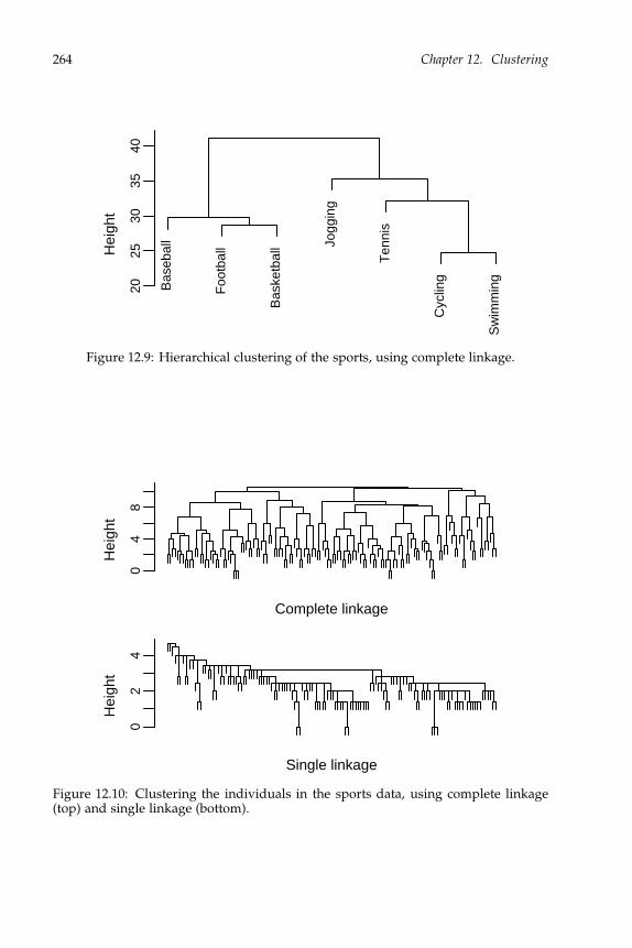
264 Chapter 12. Clustering
Bas
ebal
l
Foo
tbal
l
Bas
ketb
all Jo
ggin
g
Ten
nis
Cyc
ling
Sw
imm
ing
2025
3035
40
Hei
ght
Figure 12.9: Hierarchical clustering of the sports, using complete linkage.
04
8
Complete linkage
Hei
ght
02
4
Single linkage
Hei
ght
Figure 12.10: Clustering the individuals in the sports data, using complete linkage(top) and single linkage (bottom).

12.7. Exercises 265
Complete linkage tends to favor similar-sized clusters, because by using the max-imum distance, it is easier for two small clusters to get together than anything toattach itself to a large cluster. Single linkage tends to favor a few large clusters, andthe rest small, because the larger the cluster, the more likely it will be close to smallclusters. These ideas are borne out in the plot, where complete linkage yields a moretreey-looking dendrogram.
12.7 Exercises
Exercise 12.7.1. Show that |Σk| = cpk in (12.29) follows from (12.27) and (12.28).
Exercise 12.7.2. (a) Show that the EM algorithm, where we use the w(i)k ’s in (12.36) as
the estimate of P[Y = k | X = xi], rather than that in (12.33), is the K-means algorithmof Section 12.1. [Note: You have to worry only about the mean in (12.34).] (b) Show
that the limit as σ → 0 of P[Y = k | X = xi] is indeed given in (12.36), if we use the fkin (12.37) in (12.33).
Exercise 12.7.3 (Grades). This problem is to cluster the students in the grades databased on variables 2–6: homework, labs, inclass, midterms, and final. (a) Use K-means clustering for K = 2. (Use nstart=100, which is a little high, but makes sureeveryone gets similar answers.) Look at the centers, and briefly characterize theclusters. Compare the men and women (variable 1, 0=male, 1=female) on whichclusters they are in. (Be sure to take into account that there are about twice as manywomen as men.) Any differences? (b) Same question, for K = 3. (c) Same question,for K = 4. (d) Find the average silhouettes for the K = 2, 3 and 4 clusterings fromparts (a), (b) and (c). Which K has the highest average silhouette? (e) Use soft K-means to find the K = 1, 2, 3 and 4 clusterings. Which K is best according to theBIC’s? (Be aware that the BIC’s in Mclust are negative what we use.) Is it the same asfor the best K-means clustering (based on silhouettes) found in part (d)? (f) For eachof K = 2, 3, 4, compare the classifications of the data using regular K-means to that ofsoft K-means. That is, match the clusters produced by both methods for given K, andcount how many observations were differently clustered.
Exercise 12.7.4 (Diabetes). The data set diabetes [Reaven and Miller, 1979] is found inthe R package mclust. There are n = 145 subjects and four variables. The first vari-able (class) is a categorical variable indicating whether the subject has overt diabetes(symptoms are obvious), chemical diabetes (can be detected only through chemicalanalysis of the blood), or is normal (no diabetes). The other three variables are bloodmeasurements: glucose, insulin, sspg. (a) First, normalize the three blood measurementvariables so that they have means zero and variances 1:
data(diabetes)blood <− scale(diabetes[,2:4])
Use K-means to cluster the observations on the three normalized blood measurementvariables for K = 1, 2, . . . , 9. (b) Find the average silhouettes for the clusterings foundin part (a), except for K = 1. Which K would you choose based on this criterion?(c) Use model-based clustering, again with K = 1, . . . 9. Which model and K has thebest BIC? (d) For each of the two “best” clusterings in parts (b) and (c), plot eachpair of variables, indicating which cluster each point was assigned, as in Figure 12.6.Compare these to the same plots that use the class variable as the indicator. What

266 Chapter 12. Clustering
do you notice? (e) For each of the two best clusterings, find the table comparing theclusters with the class variable. Which clustering was closest to the class variable?Why do you suppose that clustering was closest? (Look at the plots.)
Exercise 12.7.5 (Iris). This question applies model-based clustering to the iris data,pretending we do not know which observations are in which species. (a) Do themodel-based clustering without any restrictions (i.e., use the defaults). Which modeland number K was best, according to BIC? Compare the clustering for this best modelto the actual species. (b) Now look at the BIC’s for the model chosen in part (a), butfor the various K’s from 1 to 9. Calculate the corresponding estimated posteriorprobabilities. What do you see? (c) Fit the same model, but with K = 3. Nowcompare the clustering to the true species.
Exercise 12.7.6 (Grades). Verify the dissimilarity matrices in (12.43) and (12.45).
Exercise 12.7.7 (Soft drinks). The data set softdrinks has 23 peoples’ ranking of 8soft drinks: Coke, Pepsi, Sprite, 7-up, and their diet equivalents. Do a hierarchicalclustering on the drinks, so that the command is
hclust(dist(t(softdrinks)))
then plot the tree with the appropriate labels. Describe the tree. Does the clusteringmake sense?
Exercise 12.7.8 (Cereal). Exercise 1.9.21 presented the cereal data (in the R data ma-trix cereal), finding the biplot. Do hierarchical clustering on the cereals, and on theattributes. Do the clusters make sense? What else would you like to know from thesedata? Compare the clusterings to the biplot. What is the advantage of the biplotrelative to the hierarchical clusterings?

Chapter 13
Principal Components and Related Techniques
Data reduction is a common goal in multivariate analysis — one has too many vari-ables, and wishes to reduce the number of them without losing much information.How to approach the reduction depends of course on the goal of the analysis. Forexample, in linear models, there are clear dependent variables (in the Y matrix) thatwe are trying to explain or predict from the explanatory variables (in the x matrix,and possibly the z matrix). Then Mallows’ Cp or cross-validation are reasonable ap-proaches. If the correlations between the Y’s are of interest, then factor analysis isappropriate, where the likelihood ratio test is a good measure of how many factorsto take. In classification, using cross-validation is a good way to decide on the vari-ables. In model-based clustering, and in fact any situation with a likelihood, one canbalance the fit and complexity of the model using something like AIC or BIC.
There are other situations in which the goal is not so clear cut as in those above;one is more interested in exploring the data, using data reduction to get a betterhandle on the data, in the hope that something interesting will reveal itself. Thereduced data may then be used in more formal models, although I recommend firstconsidering targeted reductions as mentioned in the previous paragraph, rather thanimmediately jumping to principal components.
Below we discuss principal components in more depth, then present multidimen-sional scaling, and canonical correlations.
13.1 Principal components, redux
Recall way back in Section 1.6 that the objective in principal component analysis wasto find linear combinations (with norm 1) with maximum variance. As an exploratorytechnique, principal components can be very useful, as are other projection pursuitmethods. The conceit underlying principal components is that variance is associatedwith interestingness, which may or may not hold. As long as in an exploratory mood,though, if one finds the top principal components are not particularly interesting orinterpretable, then one can go in a different direction.
But be careful not to shift over to the notion that components with low variancecan be ignored. It could very well be that they are the most important, e.g., mostcorrelated with a separate variable of interest. Using principal components as thefirst step in a process, where one takes the first few principal components to use in
267

268 Chapter 13. Principal Components, etc.
another procedure, such as clustering or classification, may or may not work out well.In particular, it makes little sense to use principal components to reduce the variablesbefore using them in a linear process such as regression, canonical correlations, orFisher’s linear discrimination. For example, in regression, we are trying to find thelinear combination of x’s that best correlates with y. The answer is given by the fit, y.Using principal components first on the x’s will give us a few new variables that arelinear combinations of x’s, which we then further take linear combinations of to cor-relate with the y. What we end up with is a worse correlation than if we just startedwith the original x’s, since some parts of the x’s are left behind. The same thinkinggoes when using linear discrimination: We want the linear combination of x’s thatbest distinguishes the groups, not the best linear combination of a few linear com-binations of the x’s. Because factor analysis tries to account for correlations amongthe variables, if one transforms to principal components, which are uncorrelated, be-fore applying factor analysis, then there will be no common factors. On the otherhand, if one is using nonlinear techniques such as classification trees, first reducingby principal components may indeed help.
Even principal components are not unique. E.g., you must choose whether ornot to take into account covariates or categorical factors before finding the samplecovariance matrix. You also need to decide how to scale the variables, i.e., whether toleave them in their original units, or scale so that all variables have the same samplevariance, or scale in some other way. The scaling will affect the principal components,unlike in a factor analysis or linear regression.
13.1.1 Example: Iris data
Recall that the Fisher-Anderson iris data (Section 1.3.1) has n = 150 observations andq = 4 variables. The measurements of the petals and sepals are in centimeters, soit is reasonable to leave the data unscaled. On the other hand, the variances of thevariables do differ, so scaling so that each has unit variance is also reasonable. Fur-thermore, we could either leave the data unadjusted in the sense of subtracting theoverall mean when finding the covariance matrix, or adjust the data for species bysubtracting from each observation the mean of its species. Thus we have four reason-able starting points for principal components, based on whether we adjust for speciesand whether we scale the variables. Figure 13.1 has plots of the first two principalcomponents for each of these possibilities. Note that there is a stark difference be-tween the plots based on adjusted and unadjusted data. The unadjusted plots showa clear separation based on species, while the adjusted plots have the species totallymixed, which would be expected because there are differences in means betweenthe species. Adjusting hides those differences. There are less obvious differencesbetween the scaled and unscaled plots within adjusted/unadjusted pairs. For the ad-justed data, the unscaled plot seems to have fairly equal spreads for the three species,while the scaled data has the virginica observations more spread out than the othertwo species.
The table below shows the sample variances, s2, and first principal component’sloadings (sample eigenvector), PC1, for each of the four sets of principal components:
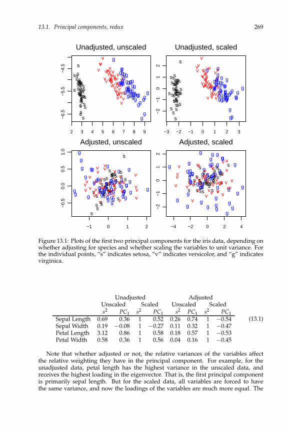
13.1. Principal components, redux 269
s
sss
s
s
ss
s
s
s
ss
s
ss
s
s
s
ssss s
sssss
ss
s
ss
ss
ss
s
ss
s
s
ss
s
s
s
s
s
v
vv
v
v
v
v
v
v
v
v
v
v
vv
v
vvvv
vvv
vvv vv
vv
vv
v vv
vv
vv
vv
v
v
v
vvv
v
v
vg
g
g
gg
g
g
g
g
g
g
g
g
gg
gg
g
g
g
g
g
g
g
gg
gg g
g g
g
gg
g
g
ggg
gg
g
g
ggg
g
gg
g
2 3 4 5 6 7 8 9
−6.
5−
5.5
−4.
5
Unadjusted, unscaled
s
sss
s
s
ss
ss
s
s
ss
s
s
s
s
ss
ss
sss
s
sssss
s
ss
ss
ss
s
ss
s
s
ss
s
s
s
s
s
vv v
v
vv
v
v
v
v
v
v
v
vv
v
vv
vv
v
vv
vvv
vv
v
vvv
v vv
vv
v
v
vv
v
v
v
vvv v
v
v
g
g
gg
gg
g
g
g
g
g
g
g
g
g
gg
g
g
g
g
g
g
g
gg
gg g
gg
g
ggg
ggg
gggg
g
ggg
g
g
g
g
−3 −2 −1 0 1 2 3
−2
−1
01
2
Unadjusted, scaled
s
s
ss
ss
ss
ss
s
s
ss
s
s
s
ss
s
s
ss
sss
sss
ss
s
ss
ss
s s
sss
s
sss
s
s
s
s
sv
v
v
vv v
vv
v
v
v
v
v
v
v
v vv
v
v
v v
v
v
vv
vv
vv
vvv
v
v
v
v
v
v
vv
v v vv
vvv
v
vgg
g gg
g
g
g g
g g
gg
g
gg
gg
g
g
g g
g
gg
g
gg
gg
g
g
gg
gg
g
g
gggg
ggg g
g
g
g
g
−1 0 1 2
−0.
50.
00.
51.
0
Adjusted, unscaled
ssss
sss
sss
ss
s
ss
ss
ss
s
s
ss
s
ss
sssss
ss
s
ss s
sss
s
s
s
s
s
sss ss
v
v
vv
vv
vv
v
v
v
v
v
v
v
v
v
v vv
v
v
vv
v v
v
vv
vvvv
v
vv
v
v
vv
vv
vv vvv
v
v
v
g
g
gg
g
g
g
gg
gg
gg
g
gg
g g
g
g
gg
g
gg
g
gg
g
g g
g
g
g
g
g
g
g
gg
gg
g g
gg
g
g
g
g
−4 −2 0 2 4
−2
−1
01
2
Adjusted, scaled
Figure 13.1: Plots of the first two principal components for the iris data, depending onwhether adjusting for species and whether scaling the variables to unit variance. Forthe individual points, “s” indicates setosa, “v” indicates versicolor, and “g” indicatesvirginica.
Unadjusted AdjustedUnscaled Scaled Unscaled Scaleds2 PC1 s2 PC1 s2 PC1 s2 PC1
Sepal Length 0.69 0.36 1 0.52 0.26 0.74 1 −0.54Sepal Width 0.19 −0.08 1 −0.27 0.11 0.32 1 −0.47Petal Length 3.12 0.86 1 0.58 0.18 0.57 1 −0.53Petal Width 0.58 0.36 1 0.56 0.04 0.16 1 −0.45
(13.1)
Note that whether adjusted or not, the relative variances of the variables affectthe relative weighting they have in the principal component. For example, for theunadjusted data, petal length has the highest variance in the unscaled data, andreceives the highest loading in the eigenvector. That is, the first principal componentis primarily sepal length. But for the scaled data, all variables are forced to havethe same variance, and now the loadings of the variables are much more equal. The

270 Chapter 13. Principal Components, etc.
2 4 6 8 10
01
23
45
6
Index
Eig
enva
lue
2 4 6 8 10
0.2
0.6
1.0
Index
log(
ratio
)Figure 13.2: The left-hand plot is a scree plot (i versus li) of the eigenvalues for theautomobile data. The right-hand plot shows i versus log(li/li+1), the successive log-proportional gaps.
opposite holds for sepal width. A similar effect is seen for the adjusted data. Thesepal length has the highest unscaled variance and highest loading in PC1, and petalwidth the lowest variance and loading. But scaled, the loadings are approximatelyequal.
Any of the four sets of principal components is reasonable. Which to use dependson what one is interested in, e.g., if wanting to distinguish between species, theunadjusted plots are likely more interesting, while when interested in relations withinspecies, adjusting make sense. In cases where the units are vastly different for thevariables, e.g., populations in thousands and areas in square miles of cities, leavingthe data unscaled is less defensible.
13.1.2 Choosing the number of principal components
One obvious question is, “How does one choose p?” Unfortunately, there is not anyvery good answer without some clear objective in mind. There are some reasonableguidelines to use, which can at least suggest which principal components to look at.Of course, nothing prevents you from looking at as many as you have time for.
The most common graphical technique for deciding on p is the scree plot, inwhich the sample eigenvalues are plotted versus their indices. (A scree is a pile ofsmall stones at the bottom of a cliff.) Consider Example 12.3.1 on the automobile data,here using the n = 96 autos with trunk space, and all q = 11 variables. Scaling thevariables so that they are have unit sample variance, we obtain the sample eigenvalues
6.210, 1.833, 0.916, 0.691, 0.539, 0.279, 0.221, 0.138, 0.081, 0.061, 0.030. (13.2)
The scree plot is the first one in Figure 13.2. Note that there is a big drop from thefirst to the second eigenvalue. There is a smaller drop to the third, then the valuesseem to level off. Other simple plots can highlight the gaps. For example, the second

13.1. Principal components, redux 271
plot in the figure shows the logarithms of the successive proportional drops via
log(ratioi) ≡ log
(li
li+1
). (13.3)
The biggest drops are again from #1 to #2, and #2 to #3, but there are almost as largeproportional drops at the fifth and tenth stages.
One may have outside information or requirements that aid in choosing the com-ponents. For examples, there may be a reason one wishes a certain number of com-ponents (say, three if the next step is a three-dimensional plot), or to have as fewcomponents as possible in order to achieve a certain percentage (e.g., 95%) of the to-tal variance. If one has an idea that the measurement error for the observed variablesis c, then it makes sense to take just the principal components that have eigenvalue
significantly greater than c2. Or, as in the iris data, all the data is accurate just to onedecimal place, so that taking c = 0.05 is certainly defensible.
To assess significance, assume that
U ∼ Wishartq(ν, Σ), and S =1
νU, (13.4)
where ν > q and Σ is invertible. Although we do not necessarily expect this dis-tribution to hold in practice, it will help develop guidelines to use. Let the spectraldecompositions of S and Σ be
S = GLG′ and Σ = ΓΛΓ′, (13.5)
where G and Γ are each orthogonal matrices, and L and Λ are diagonal with nonin-creasing diagonal elements (the eigenvalues), as in Theorem 1.1. The eigenvalues ofS will be distinct with probability 1. If we assume that the eigenvalues of Σ are alsodistinct, then Theorem 13.5.1 in Anderson [2003] shows that for large ν, the sample
eigenvalues are approximately independent, and li ≈ N(λi, 2λ2i /ν). If components
with λi ≤ c2 are ignorable, then it is reasonable to ignore the li for which
√ν
li − c2
√2 li
< 2, equivalently, li <c2
1 − 2√
2/√
ν. (13.6)
(One may be tempted to take c = 0, but if any λi = 0, then the corresponding li willbe zero as well, so that there is no need for hypothesis testing.) Other test statistics(or really “guidance statistics”) can be easily derived, e.g., to see whether the average
of the k smallest eigenvalues are less than c2, or the sum of the first p are greater thansome other cutoff.
13.1.3 Estimating the structure of the component spaces
If the eigenvalues of Σ are distinct, then the spectral decomposition (13.5) splitsthe q-dimensional space into q orthogonal one-dimensional spaces. If, say, the firsttwo eigenvalues are equal, then the first two subspaces are merged into one two-dimensional subspace. That is, there is no way to distinguish between the top twodimensions. At the extreme, if all eigenvalues are equal, in which case Σ = λIq, thereis no statistically legitimate reason to distinguish any principal components. Moregenerally, suppose there are K distinct values among the λi’s, say
α1 > α2 > · · · > αK , (13.7)
272 Chapter 13. Principal Components, etc.
where qk of the λi’s are equal to αk:
λ1 = · · · = λq1 = α1,
λq1+1 = · · · = λq1+q2 = α2,
...
λq1+···+qK−1+1 = · · · = λq = αK . (13.8)
Then the space is split into K orthogonal subspaces, of dimensions q1, . . . , qK,where q = q1 + · · · + qK. See Exercise 13.4.3. The vector (q1, . . . , qK) is referredto as the pattern of equalities among the eigenvalues. Let Γ be an orthogonal matrixcontaining eigenvectors as in (13.5), and partition it as
Γ =(
Γ1 Γ2 · · · ΓK
), Γk is q × qk, (13.9)
so that Γk contains the eigenvectors for the qk eigenvalues that equal αk. These arenot unique because ΓkJ for any qk × qk orthogonal matrix J will also yield a set ofeigenvectors for those eigenvalues. The subspaces have corresponding projectionmatrices P1, . . . , PK, which are unique, and we can write
Σ =K
∑k=1
αkPk, where Pk = ΓkΓ′k. (13.10)
With this structure, the principal components can be defined only in groups, i.e., thefirst q1 of them represent one group, which have higher variance than the next groupof q2 components, etc., down to the final qK components. There is no distinctionwithin a group, so that one would take either the top q1 components, or the topq1 + q2, or the top q1 + q2 + q3, etc.
Using the distributional assumption (13.4), we find the Bayes information criterionto choose among the possible patterns (13.8) of equality. The best set can then be usedin plots such as in Figure 13.3, where the gaps will be either enhanced (if large) oreliminated (if small). The model (13.8) will be denoted M(q1,...,qK). Anderson [1963]
(see also Section 13.1.6) shows the following.
Theorem 13.1. Suppose (13.4) holds, and S and Σ have spectral decompositions as in (13.5).
Then the MLE of Σ under the model M(q1,...,qK) is given by Σ = GΛG′, where the λi’s are
found by averaging the relevant li’s:
λ1 = . . . = λq1 = α1 =1
q1(l1 + . . . + lq1),
λq1+1 = · · · = λq1+q2 = α2 =1
q2(lq1+1 + · · ·+ lq1+q2),
...
λq1+···+qK−1+1 = · · · = λq = αK =1
qK(lq1+···+qK−1+1 + · · ·+ lq). (13.11)
The number of free parameters is
d(q1, . . . qK) =1
2(q2 −
K
∑k=1
q2k) + K. (13.12)

13.1. Principal components, redux 273
The deviance can then be taken to be
deviance(M(q1,...qK)(Σ) ; S) = νq
∑i=1
log(λi) = νK
∑k=1
qk log(αk). (13.13)
See Exercise 13.4.4. Using (13.12), we have
BIC(M(q1,...qK)) = νK
∑k=1
qk log(αk) + log(ν)d(q1, . . . qK). (13.14)
13.1.4 Example: Automobile data
Let S be the scaled covariance matrix for the automobiles with trunks, described inSection 12.3.1. Equation (13.2) and Figure 13.2 exhibit the eigenvalues of S. They aredenoted lj in (13.15). We first illustrate the model (13.8) with pattern (1, 1, 3, 3, 2, 1).The MLE’s of the eigenvalues are then found by averaging the third through fifth,the sixth through eighth, the ninth and tenth, and leaving the others alone, denoted
below by the λj’s:
j 1 2 3 4 5lj 6.210 1.833 0.916 0.691 0.539
λj 6.210 1.833 0.716 0.716 0.716
j 6 7 8 9 10 11lj 0.279 0.221 0.138 0.081 0.061 0.030
λj 0.213 0.213 0.213 0.071 0.071 0.030
(13.15)
With ν = n − 1 = 95,
deviance(M(1,1,3,3,2,1)(Σ) ; S) = 95 ∑j
log(λj) = −1141.398, (13.16)
and d(1, 1, 3, 3, 2, 1) = 54, hence
BIC(M(1,1,3,3,2,1)) = −1141.398 + log(95) 54 = −895.489. (13.17)
Table 13.1.4 contains a number of models, one each for K from 1 to 11. Eachpattern after the first was chosen to be the best that is obtained from the previous bysumming two consecutive qk’s. The estimated probabilities are among those in thetable. Clearly, the preferred is the one with MLE in (13.15). Note that the assumption(13.4) is far from holding here, both because the data are not normal, and becausewe are using a correlation matrix rather than a covariance matrix. We are hoping,though, that in any case, the BIC is a reasonable balance of the fit of the model on theeigenvalues and the number of parameters.
Figure 13.3 shows the scree plots, using logs, of the sample eigenvalues and thefitted ones from the best model. Note that the latter gives more aid in deciding howmany components to choose because the gaps are enhanced or eliminated. That is,taking one or two components is reasonable, but because there is little distinction

274 Chapter 13. Principal Components, etc.
Pattern d BIC BIC PBIC
(1, 1, 1, 1, 1, 1, 1, 1, 1, 1, 1) 66 −861.196 34.292 0.000(1, 1, 1, 1, 1, 2, 1, 1, 1, 1) 64 −869.010 26.479 0.000(1, 1, 1, 2, 2, 1, 1, 1, 1) 62 −876.650 18.839 0.000(1, 1, 3, 2, 1, 1, 1, 1) 59 −885.089 10.400 0.004(1, 1, 3, 2, 1, 2, 1) 57 −892.223 3.266 0.159(1, 1, 3, 3, 2, 1) 54 −895.489 0.000 0.812(1, 1, 3, 3, 3) 51 −888.502 6.987 0.025(1, 4, 3, 3) 47 −870.824 24.665 0.000(1, 4, 6) 37 −801.385 94.104 0.000(5, 6) 32 −657.561 237.927 0.000
11 1 4.554 900.042 0.000
Table 13.1: The BIC’s for the sequence of principal component models for the auto-mobile data.
2 4 6 8 10
−3
−1
12
Sample
Index
log(
eige
nval
ue)
2 4 6 8 10
−3
−1
12
MLE
Index
log(
eige
nval
ue)
Figure 13.3: Plots of j versus the sample lj’s, and j versus the MLE λj’s, for the chosenmodel.
among the next three, one may as well take all or none of those three. Similarly withnumbers six, seven and eight.
What about interpretations? Below we have the first five principal component
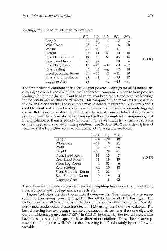
13.1. Principal components, redux 275
loadings, multiplied by 100 then rounded off:
PC1 PC2 PC3 PC4 PC5
Length 36 −23 3 −7 26Wheelbase 37 −20 −11 6 20Width 35 −29 19 −11 1Height 25 41 −41 10 −10Front Head Room 19 30 68 45 −16Rear Head Room 25 47 1 28 6Front Leg Room 10 −49 −30 69 −37Rear Seating 30 26 −43 2 18Front Shoulder Room 37 −16 20 −11 10Rear Shoulder Room 38 −1 7 −13 12Luggage Area 28 6 −2 −43 −81
(13.18)
The first principal component has fairly equal positive loadings for all variables, in-dicating an overall measure of bigness. The second component tends to have positiveloadings for tallness (height, front head room, rear head room), and negative loadingsfor the length and width-type variables. This component then measures tallness rela-tive to length and width. The next three may be harder to interpret. Numbers 3 and 4could be front seat versus back seat measurements, and number 5 is mainly luggagespace. But from the analysis in (13.15), we have that from a statistical significancepoint of view, there is no distinction among the third through fifth components, thatis, any rotation of them is equally important. Thus we might try a varimax rotationon the three vectors, to aid in interpretation. (See Section 10.3.2 for a description ofvarimax.) The R function varimax will do the job. The results are below:
PC∗3 PC∗
4 PC∗5
Length −4 −20 18Wheelbase −11 0 21Width 13 −17 −6Height −32 29 −1Front Head Room 81 15 7Rear Head Room 11 18 19Front Leg Room 4 83 6Rear Seating −42 10 18Front Shoulder Room 12 −22 1Rear Shoulder Room 0 −19 3Luggage Area −4 8 −92
(13.19)
These three components are easy to interpret, weighting heavily on front head room,front leg room, and luggage space, respectively.
Figure 13.4 plots the first two principal components. The horizontal axis repre-sents the size, going from the largest at the left to the smallest at the right. Thevertical axis has tall/narrow cars at the top, and short/wide at the bottom. We alsoperformed model-based clustering (Section 12.3) using just these two variables. Thebest clustering has two groups, whose covariance matrices have the same eigenval-ues but different eigenvectors (“EEV” in (12.31)), indicated by the two ellipses, whichhave the same size and shape, but have different orientations. These clusters are rep-resented in the plot as well. We see the clustering is defined mainly by the tall/widevariable.
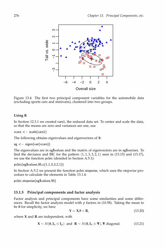
276 Chapter 13. Principal Components, etc.
−6 −4 −2 0 2 4
−3
−1
01
23
Overall size
Tal
l vs.
wid
e
Figure 13.4: The first two principal component variables for the automobile data(excluding sports cars and minivans), clustered into two groups.
Using R
In Section 12.3.1 we created cars1, the reduced data set. To center and scale the data,so that the means are zero and variances are one, use
xcars <− scale(cars1)
The following obtains eigenvalues and eigenvectors of S:
eg <− eigen(var(xcars))
The eigenvalues are in eg$values and the matrix of eigenvectors are in eg$vectors. Tofind the deviance and BIC for the pattern (1, 1, 3, 3, 2, 1) seen in (13.15) and (13.17),we use the function pcbic (detailed in Section A.5.1):
pcbic(eg$values,95,c(1,1,3,3,2,1))
In Section A.5.2 we present the function pcbic.stepwise, which uses the stepwise pro-cedure to calculate the elements in Table 13.1.4:
pcbic.stepwise(eg$values,95)
13.1.5 Principal components and factor analysis
Factor analysis and principal components have some similarities and some differ-ences. Recall the factor analysis model with p factors in (10.58). Taking the mean tobe 0 for simplicity, we have
Y = Xβ + R, (13.20)
where X and R are independent, with
X ∼ N(0, In ⊗ Ip) and R ∼ N(0, In ⊗ Ψ), Ψ diagonal. (13.21)
13.1. Principal components, redux 277
For principal components, where we take the first p components, partition Γ andΛ in (13.5) as
Γ =(
Γ1 Γ2
)and Λ =
(Λ1 00 Λ2
). (13.22)
Here, Γ1 is q × p, Γ2 is q × (q − p), Λ1 is p × p, and Λ2 is (q − p)× (q − p), the Λk’sbeing diagonal. The large eigenvalues are in Λ1, the small ones are in Λ2. BecauseIq = ΓΓ
′ = Γ1Γ′1 + Γ2Γ
′2, we can write
Y = YΓ1Γ′1 + YΓ2Γ
′2 = Xβ+ R, (13.23)
where
X = YΓ1 ∼ N(0, ΣX), β = Γ′1, and R = YΓ2Γ
′2 ∼ N(0, In ⊗ ΣR). (13.24)
Because Γ′1Γ2 = 0, X, and R are again independent. We also have (Exercise 13.4.5)
ΣX = Γ′1ΓΛΓ
′Γ1 = Λ1, and ΣR = Γ2Γ
′2ΓΛΓ
′Γ2Γ
′2 = Γ2Λ2Γ
′2. (13.25)
Comparing these covariances to the factor analytic ones in (13.20), we see the follow-ing:
ΣX ΣR
Factor analysis Ip Ψ
Principal components Λ1 Γ2Λ2Γ′2
(13.26)
The key difference is in the residuals. Factor analysis chooses the p-dimensional X sothat the residuals are uncorrelated, though not necessarily small. Thus the correlationsamong the Y’s are explained by the factors X. Principal components chooses the p-dimensional X so that the residuals are small (the variances sum to the sum of the(q − p) smallest eigenvalues), but not necessarily uncorrelated. Much of the varianceof the Y is explained by the components X.
A popular model that fits into both frameworks is the factor analytic model (13.20)with the restriction that
Ψ = σ2Iq, σ2 “small.” (13.27)
The interpretation in principal components is that the X contains the important infor-mation in Y, while the residuals R contain just random measurement error. For factoranalysis, we have that the X explains the correlations among the Y, and the residualshappen to have the same variances. In this case, we have
Σ = βΣXXβ′ + σ2Iq. (13.28)
Because β is q × p, there are at most p positive eigenvalues for βΣXXβ′. Call these
λ∗1 ≥ λ∗
2 ≥ · · · ≥ λ∗p, and let Λ
∗1 be the p× p diagonal matrix with diagonals λ∗
i . Then
the spectral decomposition is
βΣXXβ′ = Γ
(Λ∗1 0
0 0
)Γ′ (13.29)
for some orthogonal Γ. But any orthogonal matrix contains eigenvectors for Iq = ΓΓ′,
hence Γ is also an eigenvector matrix for Σ:
Σ = ΓΛΓ′ = Γ
(Λ∗1 + σ2Ip 0
0 σ2Iq−p
)Γ′. (13.30)

278 Chapter 13. Principal Components, etc.
Thus the eigenvalues of Σ are
λ∗1 + σ2 ≥ λ∗
2 + σ2 ≥ · · · ≥ λ∗p + σ2 ≥ σ2 = · · · = σ2, (13.31)
and the eigenvectors for the first p eigenvalues are the columns of Γ1. In this case thefactor space and the principal component space are the same. In fact, if the λ∗
j are
distinct and positive, the eigenvalues (13.30) satisfy the structural model (13.8) withpattern (1, 1, . . . , 1, q − p). A common approach to choosing p in principal compo-nents is to use hypothesis testing on such models to find the smallest p for which themodel fits. See Anderson [1963] or Mardia, Kent, and Bibby [1979]. Of course, AICor BIC could be used as well.
13.1.6 Justification of the principal component MLE
We first find the MLE of Σ, and the maximal value of the likelihood, for U as in (13.4),where the eigenvalues of Σ satisfy (13.8). We know from (10.1) that the likelihood forS is
L(Σ ; S) = |Σ|−ν/2 e−ν2 trace(Σ
−1S). (13.32)
For the general model, i.e., where there is no restriction among the eigenvalues of Σ
(M(1,1,...,1)), the MLE of Σ is S.
Suppose there are nontrivial restrictions (13.8). Write Σ and S in their spectraldecomposition forms (13.5) to obtain
L(Σ ; S) = |Λ|−ν/2 e−ν2 trace((ΓΛΓ
′)−1GLG′)
= (∏ λi)−ν/2 e−
12 trace(Λ
−1Γ′GLG′
Γ). (13.33)
Because of the multiplicities in the eigenvalues, the Γ is not uniquely determinedfrom Σ, but any orthogonal matrix that maximizes the likelihood is adequate.
We start by fixing Λ, and maximizing the likelihood over the Γ. Set
F = G′Γ, (13.34)
which is also orthogonal, and note that
− 1
2trace(Λ−1F′LF) = − 1
2
q
∑i=1
q
∑j=1
f 2ij
li
λj
=q
∑i=1
q
∑j=1
f 2ij liβj −
1
2λq
q
∑i=1
li, (13.35)
where
βj = − 1
2λj+
1
2λq. (13.36)
(The 1/(2λq) is added because we need the βj’s to be nonnegative in what follows.)Note that the last term in (13.35) is independent of F. We do summation by parts byletting
di = li − li+1, δi = βi − βi+1, 1 ≤ i ≤ q − 1, dq = lq, δq = βq, (13.37)
13.1. Principal components, redux 279
so that
li =q
∑k=i
dk and βj =q
∑m=j
δm. (13.38)
Because the li’s and λi’s are nondecreasing in i, the li’s are positive, and by (13.36)the βj’s are also nonnegative, we have that the δi’s and di’s are all nonnegative. Using(13.38) and interchanging the orders of summation, we have
q
∑i=1
q
∑j=1
f 2ij liβj =
q
∑i=1
q
∑j=1
q
∑k=i
q
∑m=j
f 2ij dkδm
=q
∑k=1
q
∑m=1
dkδm
k
∑i=1
m
∑j=1
f 2ij. (13.39)
Because F is an orthogonal matrix,
k
∑i=1
m
∑j=1
f 2ij ≤ mink, m. (13.40)
Also, with F = Iq, the fii = 1, hence expression in (13.40) is an equality. By thenonnegativity of the dk’s and δm’s, the sum in (13.39), hence in (13.35), is maximized(though not uniquely) by taking F = Iq. Working back, from (13.34), the (not neces-sarily unique) maximizer over Γ of (13.35) is
Γ = G. (13.41)
Thus the maximum over Γ in the likelihood (13.33) is
L(GΛG′ ; S) = (∏ λi)−ν/2e−
ν2 ∑(li/λi). (13.42)
Break up the product according to the equalities (13.8):
K
∏k=1
α−qkν/2k e−
ν2 (tk/αk), (13.43)
where
t1 =q1
∑i=1
li and tk =q1+···+qk
∑i=q1+···+qk−1+1
li for 2 ≤ k ≤ K. (13.44)
It is easy to maximize over each αk in (13.43), which proves that (13.11) is indeed theMLE of the eigenvalues. Thus with (13.41), we have the MLE of Σ as in Theorem 13.1.
We give a heuristic explanation of the dimension (13.12) of the model M(q1,...qK) in
(13.8). To describe the model, we need the K distinct parameters among the λi’s, aswell as the K orthogonal subspaces that correspond to the distinct values of λi. Westart by counting the number of free parameters needed to describe an s-dimensionalsubspace of a t-dimensional space, s < t. Any such subspace can be described by at × s basis matrix B, that is, the columns of B comprise a basis for the subspace. (SeeSection 5.2.) The basis is not unique, in that BA for any invertible s × s matrix A isalso a basis matrix, and in fact any basis matrix equals BA for some such A. Take A
280 Chapter 13. Principal Components, etc.
to be the inverse of the top s× s submatrix of B, so that BA has Is as its top s × s part.This matrix has (t − s)× s free parameters, represented in the bottom (t − s)× s partof it, and is the only basis matrix with Is at the top. Thus the dimension is (t − s)× s.(If the top part of B is not invertible, then we can find some other subset of s rows touse.)
Now for model (13.8), we proceed stepwise. There are q1(q2 + · · ·+ qK) parame-ters needed to specify the first q1-dimensional subspace. Next, focus on the subspaceorthogonal to that first one. It is (q2 + · · ·+ qK)-dimensional, hence to describe thesecond, q2-dimensional, subspace within that, we need q2 × (q3 + · · ·+ qK) parame-ters. Continuing, the total number of parameters is
q1(q2 + · · ·+ qK) + q2(q3 + · · ·+ qK) + · · ·+ qK−1qk =1
2(q2 −
K
∑k=1
q2k). (13.45)
Adding K for the distinct λi’s, we obtain the dimension in (13.12).
13.2 Multidimensional scaling
Given n objects and defined distances, or dissimilarities, between them, multidimen-sional scaling tries to mimic the dissimilarities as close as possible by representingthe objects in p-dimensional Euclidean space, where p is fairly small. That is, sup-
pose o1, . . . , on are the objects, and d(oi, oj) is the dissimilarity between the ith and
jth objects, as in (12.15). Let ∆ be the n × n matrix of d2(oi, oj)’s. The goal is to find1 × p vectors x1, . . . , xn so that
∆ij = d2(oi, oj) ≈ ‖xi − xj‖2. (13.46)
Then the xi’s are plotted in Rp, giving an approximate visual representation of theoriginal dissimilarities.
There are a number of approaches. Our presentation here follows that of Mar-dia, Kent, and Bibby [1979], which provides more in-depth coverage. We will startwith the case that the original dissimilarities are themselves Euclidean distances, andpresent the so-called classical solution. Next, we exhibit the classical solution whenthe distances may not be Euclidean. Finally, we briefly mention the non-metric ap-proach.
13.2.1 ∆ is Euclidean: The classical solution
Here we assume that object oi has associated a 1 × q vector yi, and let Y be the n × q
matrix with yi as the ith row. Of course, now Y looks like a regular data matrix. Itmight be that the objects are observations (people), or they are variables, in whichcase this Y is really the transpose of the usual data matrix. Whatever the case,
d2(oi, oj) = ‖yi − yj‖2. (13.47)
For any n× p matrix X with rows xi, define ∆(X) to be the n× n matrix of ‖xi − xj‖2’s,
so that (13.47) can be written ∆ = ∆(Y).The classical solution looks for xi’s in (13.46) that are based on rotations of the
yi’s, much like principal components. That is, suppose B is a q × p matrix with

13.2. Multidimensional scaling 281
orthonormal columns, and set
xi = yiB, and X = YB. (13.48)
The objective is then to choose the B that minimizes
∑ ∑1≤i<j≤n
∣∣∣‖yi − yj‖2 − ‖xi − xj‖2∣∣∣ (13.49)
over B. Exercise 13.4.10 shows that ‖yi − yj‖2> ‖xi − xj‖2, which means that the ab-
solute values in (13.49) can be removed. Also, note that the sum over the ‖yi − yj‖2 isindependent of B, and by symmetry, minimizing (13.49) is equivalent to maximizing
n
∑i=1
n
∑j=1
‖xi − xj‖2 ≡ 1′n∆(X)1n . (13.50)
The next lemma is useful in relating the ∆(Y) to the deviations.
Lemma 13.1. Suppose X is n × p. Then
∆(X) = a1′n + 1na′ − 2HnXX′Hn, (13.51)
where a is the n × 1 vector with ai = ‖xi − x‖2, x is the mean of the xi’s, and Hn is thecentering matrix (1.12).
Proof. Write
‖xi − xj‖2 = ‖(xi − x)− (xj − x)‖2
= ai − 2(HnX)i(HnX)′j + aj, (13.52)
from which we obtain (13.51).
By (13.50) and (13.51) we have
n
∑i=1
n
∑j=1
‖xi − xj‖2 = 1′n∆(X)1n
= 1′n(a1′n + 1na′ − 2HnXX′Hn)1n
= 2n1′na = 2nn
∑i=1
‖xi − x‖2, (13.53)
because Hn1n = 0. But then
n
∑i=1
‖xi − x‖2 = trace(X′HnX)
= trace(B′Y′HnYB). (13.54)
Maximizing (13.54) over B is a principal components task. That is, as in Proposition1.1, this trace is maximized by taking B = G1, the first p eigenvectors of Y′HnY. Tosummarize:

282 Chapter 13. Principal Components, etc.
Proposition 13.1. If ∆ = ∆(Y), then the classical solution of the multidimensional scaling
problem for given p is X = YG1, where the columns of G1 consist of the first p eigenvectorsof Y′HnY.
If one is interested in the distances between variables, so that the distances of in-terest are in ∆(Y′) (note the transpose), then the classical solution uses the first peigenvectors of YHqY′.
13.2.2 ∆ may not be Euclidean: The classical solution
Here, we are given only the n × n dissimilarity matrix ∆. The dissimilarities may ormay not arise from Euclidean distance on vectors yi, but the solution acts as if theydo. That is, we assume there is an n × q matrix Y such that ∆ = ∆(Y), but we do notobserve the Y, nor do we know the dimension q. The first step in the process is to
derive the Y from the ∆(Y), then we apply Proposition 13.1 to find the X.It turns out that we can assume any value of q as long as it is larger than the
values of p we wish to entertain. Thus we are safe taking q = n. Also, note that using(13.51), we can see that ∆(HnX) = ∆(X), which implies that the sample mean of Y isindeterminate. Thus we may as well assume the mean is zero, i.e.,
HnY = Y, (13.55)
so that (13.51) yields∆ = ∆(Y) = a1′n + 1na′ − 2YY′. (13.56)
To eliminate the a’s, we can pre- and post-multiply by Hn:
Hn∆Hn = Hn(a1′n + 1na′ − 2YY′)Hn = −2YY′, (13.57)
hence
YY′ = − 1
2Hn∆Hn. (13.58)
Now consider the spectral decomposition (1.33) of YY′,
YY′ = JLJ′, (13.59)
where the orthogonal J = (j1, . . . , jn) contains the eigenvectors, and the diagonal Lcontains the eigenvalues. Separating the matrices, we can take
Y = JL1/2 =( √
l1 j1
√l2 j2 · · ·
√ln jn
). (13.60)
Now we are in the setting of Section 13.2.1, hence by Proposition 13.1, we need G1,the first p eigenvectors of
Y′HnY = (JL1/2)′(JL1/2) = L1/2J′JL1/2 = L. (13.61)
But the matrix of eigenvectors is just In, hence we take the first p columns of Y in(13.60):
X =( √
l1 j1
√l2 j2 · · ·
√lp jp
). (13.62)
It could be that ∆ is not Euclidean, that is, there is no Y for which ∆ = ∆(Y).In this case, the classical solution uses the same algorithm as in equations (13.58) to(13.62). A possible glitch is that some of the eigenvalues may be negative, but if p issmall, the problem probably won’t raise its ugly head.

13.2. Multidimensional scaling 283
13.2.3 Non-metric approach
The original approach to multidimensional scaling attempts to find the X that givesthe same ordering of the observed dissimilarities, rather than trying to match theactual values of the dissimilarities. See Kruskal [1964]. That is, take the t ≡ (n
2)pairwise dissimilarities and order them:
d(oi1, oj1) ≤ d(oi2
, oj2) ≤ · · · ≤ d(oit, ojt
). (13.63)
The ideal would be to find the xi’s so that
‖xi1− xj1‖2 ≤ ‖xi2
− xj2‖2 ≤ · · · ≤ ‖xit− xjt
‖2. (13.64)
That might not be (actually probably is not) possible for given p, so instead one
finds the X that comes as close as possible, where close is measured by some “stress”function. A popular stress function is given by
Stress2(X) =∑ ∑1≤i<j≤n(‖xi − xj‖2 − d∗ij)
2
∑ ∑1≤i<j≤n‖xi − xj‖4, (13.65)
where the d∗ij’s are constants that have the same ordering as the original dissimilarities
d(oi, oj)’s in (13.63), and among such orderings minimize the stress. See Johnson andWichern [2007] for more details and some examples. The approach is “non-metric”because it does not depend on the actual d’s, but just their order.
13.2.4 Examples: Grades and sports
The examples here all start with Euclidean distance matrices, and use the classicalsolution, so everything is done using principal components.
In Section 12.6.1 we clustered the five variables for the grades data (homework,labs, inclass, midterms, final) for the n = 107 students. Here we find the multidimen-sional scaling plot. The distance between two variables is the sum of squares of thedifference in scores the people obtained for them. So we take the transpose of thedata. The following code finds the plot.
ty <− t(grades[,2:6])ty <− scale(ty,scale=F)ev <− eigen(var(ty))$vectors[,1:2]tyhat <− ty%∗%evlm <− range(tyhat)∗1.1plot(tyhat,xlim=lm,ylim=lm,xlab=’Var 1’,ylab=’Var 2’,type=’n’)text(tyhat,labels=dimnames(ty)[[1]])
To plot the variables’ names rather than points, we first create the plot with no plot-ting: type=’n’. Then text plots the characters in the labels parameters, which we giveas the names of the first dimension of ty. The results are in Figure 13.5. Notice howthe inclass variable is separated from the others, homework and labs are fairly close,and midterms and final are fairly close together, not surprisingly given the clustering.
Figure 13.5 also has the multidimensional scaling plot of the seven sports fromthe Louis Roussos sports data in Section 12.1.1, found by substituting sportsranks forgrades[,2:6] in the R code. Notice that the first variable orders the sports according

284 Chapter 13. Principal Components, etc.
−100 0 50 150
−10
00
5015
0
HW
Labs
InClassMidterms
Final
Var 1
Var
2Grades
−20 0 10 20 30
−20
010
2030
BaseBFootB
BsktBTenCycSwim
Jog
Var 1
Var
2
Sports
Figure 13.5: Multidimensional scaling plot of the grades’ variables (left) and thesports’ variables (right).
to how many people typically participate, i.e., jogging, swimming and cycling canbe done solo, tennis needs two to four people, basketball has five per team, baseballnine, and football eleven. The second variable serves mainly to separate jogging fromthe others.
13.3 Canonical correlations
Testing the independence of two sets of variables in the multivariate normal dis-tribution is equivalent to testing their covariance is zero, as in Section 10.2. Whenthere is no independence, one may wish to know where the lack of independencelies. A projection-pursuit approach is to find the linear combination of the first setthat is most highly correlated with a linear combination of the second set, hopingto isolate the factors within each group that explain a substantial part of the overallcorrelations.
The distributional assumption is based on partitioning the 1 × q vector Y into Y1(1 × q1) and Y2 (1 × q2), with
Y =(
Y1 Y2)∼ N(µ, Σ), where Σ =
(Σ11 Σ12Σ21 Σ22
), (13.66)
Σ11 is q1 × q1, and Σ22 is q2 × q2. If α (q1 × 1) and β (q2 × 1) are coefficient vectors,then
Cov[Y1α, Y2β] = α′Σ12β,
Var[Y1α] = α′Σ11α, and
Var[Y2β] = β′Σ22β, (13.67)
hence
Corr[Y1α, Y2β] =α′
Σ12β√α′Σ11α β
′Σ22β. (13.68)
13.3. Canonical correlations 285
Analogous to principal component analysis, the goal in canonical correlation analysisis to maximize the correlation (13.68) over α and β. Equivalently, we could maximizethe covariance α′
Σ12β in (13.68) subject to the two variances equaling one. This pairof linear combination vectors may not explain all the correlations between Y1 and Y2,hence we next find the maximal correlation over linear combinations uncorrelatedwith the first combinations. We continue, with each pair maximizing the correlationsubject to being uncorrelated with the previous.
The precise definition is below. Compare it to Definition 1.2 for principal compo-nents.
Definition 13.1. Canonical correlations. Assume (Y1, Y2) are as in (13.66), where Σ11and Σ22 are invertible, and set m = minq1, q2. Let α1, . . . ,αm be a set of q1 × 1 vectors,and β1, . . . ,βm be a set of q2 × 1 vectors, such that
(α1,β1) is any (α,β) that maximizes α′Σ12β over α′
Σ11α = β′Σ22β = 1;
(α2,β2) is any (α,β) that maximizes α′Σ12β over α′
Σ11α = β′Σ22β = 1,
α′Σ11α1 = β′
Σ22β1 = 0;
...
(αm,βm) is any (α,β) that maximizes α′Σ12β over α′
Σ11α = β′Σ22β = 1,
α′Σ11αi = β
′Σ22βi = 0,
i = 1, . . . , m − 1. (13.69)
Then δi ≡ α′iΣ12βi is the ith canonical correlation, and αi and βi are the associated
canonical correlation loading vectors.
Recall that principal component analysis (Definition 1.2) led naturally to the spec-tral decomposition theorem (Theorem 1.1). Similarly, canonical correlation analysiswill lead to the singular value decomposition (Theorem 13.2 below). We begin thecanonical correlation analysis with some simplifications. Let
ψi = Σ1/211 αi and γi = Σ
1/222 βi (13.70)
for each i, so that the γi’s and ψi’s are sets of orthonormal vectors, and
δi = Corr[Y1αi, Y2βi] = ψ′i Ξγi, (13.71)
where
Ξ = Σ−1/211 Σ12Σ
−1/222 . (13.72)
This matrix Ξ is a multivariate generalization of the correlation coefficient which isuseful here, but I don’t know exactly how it should be interpreted.
In what follows, we assume that q1 ≥ q2 = m. The q1 < q2 case can be handledsimilarly. The matrix Ξ
′Ξ is a q2 × q2 symmetric matrix, hence by the spectral decom-
position in (1.33), there is a q2 × q2 orthogonal matrix Γ and a q2 × q2 diagonal matrixΛ with diagonal elements λ1 ≥ λ2 ≥ · · · ≥ λq2 such that
Γ′Ξ′ΞΓ = Λ. (13.73)

286 Chapter 13. Principal Components, etc.
Let γ1, . . . ,γq2 denote the columns of Γ, so that the ith column of ΞΓ is Ξγi. Then(13.73) shows these columns are orthogonal and have squared lengths equal to theλi’s, i.e.,
‖Ξγi‖2 = λi and (Ξγi)′(Ξγj) = 0 if i 6= j. (13.74)
Furthermore, because the γi’s satisfy the equations for the principal components’loading vectors in (1.28) with S = Ξ
′Ξ,
‖Ξγi‖ =√
λi maximizes ‖Ξγ‖ over ‖γ‖ = 1,γ ′γj = 0 for j < i. (13.75)
Now for the first canonical correlation, we wish to find unit vectors ψ and γ tomaximize ψ′
Ξγ. By Corollary 8.2, for γ fixed, the maximum over ψ is when ψ isproportional to Ξγ, hence
ψ′Ξγ ≤ ‖Ξγ‖, equality achieved with ψ =
Ξγ
‖Ξγ‖ . (13.76)
But by (13.75), ‖Ξγ‖ is maximized when γ = γ1, hence
ψ′Ξγ ≤ ψ′
1Ξγ1 =√
λ1, ψ1 =Ξγ1
‖Ξγ1‖. (13.77)
Thus the first canonical correlation δ1 is√
λ1. (The ψ1 is arbitrary if λ1 = 0.)We proceed for i = 2, . . . , k, where k is the index of the last positive eigenvalue,
i.e., λk > 0 = λk+1 = · · · = λq2 . For the ith canonical correlation, we need to find unitvectors ψ orthogonal to ψ1, . . . ,ψi−1, and γ orthogonal to γ1, . . . ,γi−1, that maximizeψ′
Ξγ. Again by (13.75), the best γ is γi, and the best ψ is proportional to Ξγi, so that
ψ′Ξγ ≤ ψ′
i Ξγi =√
λi ≡ δi, ψi =Ξγi
‖Ξγi‖. (13.78)
That this ψi is indeed orthogonal to previous ψj’s follows from the second equationin (13.74).
If λi = 0, then ψ′Ξγi = 0 for any ψ. Thus the canonical correlations for i > k
are δi = 0, and the corresponding ψi’s, i > k, can be any set of vectors such thatψ1, . . . ,ψq2 are orthonormal.
Finally, to find the αi andβi in (13.69), we solve the equations in (13.70):
αi = Σ−1/211 ψi and βi = Σ
−1/222 γi , i = 1, . . . , m. (13.79)
Backing up a bit, we have almost obtained the singular value decomposition of Ξ.Note that by (13.78), δi = ‖Ξγi‖, hence we can write
ΞΓ =(
Ξγ1 · · · Ξγq2
)
=(ψ1δ1 · · · ψq2 δq2
)
= Ψ∆, (13.80)
where Ψ = (ψ1, . . . ,ψq2 ) has orthonormal columns, and ∆ is diagonal with δ1, . . . , δq2
on the diagonal. Shifting the Γ to the other side of the equation, we obtain thefollowing.

13.3. Canonical correlations 287
Theorem 13.2. Singular value decomposition. The q1 × q2 matrix Ξ can be written
Ξ = Ψ∆Γ′ (13.81)
where Ψ (q1 × m) and Γ (q2 × m) have orthonormal columns, and ∆ is an m × m diagonalmatrix with diagonals δ1 ≥ δ2 ≥ · · · ≥ δm ≥ 0, where m = minq1, q2.
To summarize:
Corollary 13.1. Let (13.81) be the singular value decomposition of Ξ = Σ−1/211 Σ12Σ
−1/222 for
model (13.66). Then for 1 ≤ i ≤ minq1, q2, the ith canonical correlation is δi, with loading
vectors αi and βi given in (13.79), where ψi (γi) is the ith column of Ψ (Γ).
Next we present an example, where we use the estimate of Σ to estimate thecanonical correlations. Theorem 13.3 guarantees that the estimates are the MLE’s.
13.3.1 Example: Grades
Return to the grades data. In Section 10.3.3, we looked at factor analysis, finding twomain factors: An overall ability factor, and a contrast of homework and labs versusmidterms and final. Here we lump in inclass assignments with homework and labs,and find the canonical correlations between the sets (homework, labs, inclass) and(midterms, final), so that q1 = 3 and q2 = 2. The Y is the matrix of residuals from themodel (10.80). In R,
x <− cbind(1,grades[,1])y <− grades[,2:6]−x%∗%solve(t(x)%∗%x,t(x))%∗%grades[,2:6]s <− t(y)%∗%y/(nrow(y)−2)corr <− cov2cor(s)
The final statement calculates the correlation matrix from the S, yielding
HW Labs InClass Midterms FinalHW 1.00 0.78 0.28 0.41 0.40Labs 0.78 1.00 0.42 0.38 0.35InClass 0.28 0.42 1.00 0.24 0.27Midterms 0.41 0.38 0.24 1.00 0.60Final 0.40 0.35 0.27 0.60 1.00
(13.82)
There are q1 × q2 = 6 correlations between variables in the two sets. Canonical
correlations aim to summarize the overall correlations by the two δi’s. The estimateof the Ξ matrix in (13.69) is given by
Ξ = S−1/211 S12S−1/2
22
=
0.236 0.2540.213 0.1460.126 0.185
, (13.83)
found in R using
symsqrtinv1 <− symsqrtinv(s[1:3,1:3])symsqrtinv2 <− symsqrtinv(s[4:5,4:5])xi <− symsqrtinv1%∗%s[1:3,4:5]%∗%symsqrtinv2
288 Chapter 13. Principal Components, etc.
where
symsqrtinv <− function(x) ee <− eigen(x)ee$vectors%∗%diag(sqrt(1/ee$values))%∗%t(ee$vectors)
calculates the inverse symmetric square root of an invertible symmetric matrix x. Thesingular value decomposition function in R is called svd:
sv <− svd(xi)a <− symsqrtinv1%∗%sv$ub <− symsqrtinv2%∗%sv$v
The component sv$u is the estimate of Ψ and the component sv$v is the estimate of Γ
in (13.81). The matrices of loading vectors are obtained as in (13.79):
A = S−1/211 Ψ =
−0.065 0.059−0.007 −0.088−0.014 0.039
,
and B = S−1/222 Γ =
(−0.062 −0.12−0.053 0.108
). (13.84)
The estimated canonical correlations (singular values) are in the vector sv$d, whichare
d1 = 0.482 and d2 = 0.064. (13.85)
The d1 is fairly high, and d2 is practically negligible. (See the next section.) Thus itis enough to look at the first columns of A and B. We can change signs, and take thefirst loadings for the first set of variables to be (0.065, 0.007, 0.014), which is primarilythe homework score. For the second set of variables, the loadings are (0.062, 0.053),essentially a straight sum of midterms and final. Thus the correlations among the twosets of variables can be almost totally explained by the correlation between homeworkand the sum of midterms and final, which correlation is 0.45, versus the optimum of0.48.
13.3.2 How many canonical correlations are positive?
One might wonder how many of the δi’s are nonzero. We can use BIC to get an idea.The model is based on the usual
S =1
νU, where U ∼ Wishartq(ν, Σ), (13.86)
ν ≥ q, with Σ partitioned as in (13.66), and S partitioned similarly. Let Ψ∆Γ′ in (13.81)
be the singular value decomposition of Ξ as in (13.72). Then model K (1 ≤ K ≤ m ≡minq1, q2) is given by
MK : δ1 ≥ δ2 ≥ · · · ≥ δK > δK+1 = · · · = δm = 0, (13.87)
where the δi’s are the canonical correlations, i.e., diagonals of ∆. Let
S−1/211 S12S−1/2
22 = PDG′ (13.88)

13.3. Canonical correlations 289
be the sample analog of Ξ (on the left), and its singular value decomposition (on theright).
We first obtain the MLE of Σ under model K. Note that Σ and (Σ11, Σ22, Ξ) arein one-to-one correspondence. Thus it is enough to find the MLE of the latter set ofparameters. The next theorem is from Fujikoshi [1974].
Theorem 13.3. For the above setup, the MLE of (Σ11, Σ22, Ξ) under model MK in (13.87)is given by
(S11, S22, PD(K)G′), (13.89)
where D(K) is the diagonal matrix with diagonals (d1, d2, . . . , dK , 0, 0, . . . , 0).
That is, the MLE is obtained by setting to zero the sample canonical correlationsthat are set to zero in the model. One consequence of the theorem is that the natu-ral sample canonical correlations and accompanying loading vectors are indeed theMLE’s. The deviance, for comparing the models MK, can be expressed as
deviance(MK) = νK
∑i=1
log(1 − d2i ). (13.90)
See Exercise 13.4.15.For the BIC, we need the dimension of the model. The number of parameters for
the Σii’s we know to be qi(qi + 1)/2. For Ξ, we look at the singular value decompo-sition (13.81):
Ξ = Ψ∆(K)
Γ′ =
K
∑i=1
δiψiγ′i . (13.91)
The dimension for the δi’s is K. Only the first K of the ψi’s enter into the equation.Thus the dimension is the same as for principal components with K distinct eigen-values, and the rest equal at 0, yielding pattern (1, 1, . . . , 1, q1 − K), where there areK ones. Similarly, the γi’s dimension is as for pattern (1, 1, . . . , 1, q2 − K). Then by(13.45),
dim(Γ) + dim(Ψ) + dim(∆(K)) =1
2(q2
1 − K − (q1 − K)2)
+1
2(q2
2 − K − (q2 − K)2) + K
=K(q − K). (13.92)
Finally, we can take
BIC(MK) = νK
∑k=1
log(1 − d2k) + log(ν)K(q − K) (13.93)
because the qi(qi + 1)/2 parts are the same for each model.In the example, we have three models: K = 0, 1, 2. K = 0 means the two sets
of variables are independent, which we already know is not true, and K = 2 is theunrestricted model. The calculations, with ν = 105, d1 = 0.48226 and d2 = 0.064296:
K Deviance dim(Ξ) BIC PBIC
0 0 0 0 0.00991 −27.7949 4 −9.1791 0.97852 −28.2299 6 −0.3061 0.0116
(13.94)
Clearly K = 1 is best, which is what we figured above.
290 Chapter 13. Principal Components, etc.
13.3.3 Partial least squares
A similar idea is to find the linear combinations of the variables to maximize thecovariance, rather than correlation:
Cov[Y1a, Y2b] = a′Σ12b. (13.95)
The process is the same as for canonical correlations, but we use the singular valuedecomposition of Σ12 instead of Ξ. The procedure is called partial least squares,but it could have been called canonical covariances. It is an attractive alternative tocanonical correlations when there are many variables and not many observations, inwhich cases the estimates of Σ11 and Σ22 are not invertible.
13.4 Exercises
Exercise 13.4.1. In the model (13.4), find the approximate test for testing the nullhypothesis that the average of the last k (k < q) eigenvalues is less than the constant
c2.
Exercise 13.4.2. Verify the expression for Σ in (13.10).
Exercise 13.4.3. Consider the q × q covariance matrix Σ = ΓΛΓ′ as in the discussion
from (13.7) to (13.10), where there are qk eigenvalues equal to αk. For each k, let Akbe the set of all eigenvectors corresponding to the eigenvalue αk, plus the 0 vector.That is,
Ak = v | Σv = αkv. (13.96)
(a) Substituting u = Γ′v, show that Ak = Γu | Λu = αku. Argue that u satisfies
the given condition if and only if the only nonzero components of u are uq1+···+qk−1+1to uq1+···+qk
, i.e., those with indices i such that λi = αk. (b) Show that thereforeAk = spancolumns of Γk, and that Pk in (13.10) is its projection matrix. (c) Supposeqk = 1, i.e., λi = αk for a single i. Show that the only eigenvectors corresponding to
αk with norm 1 are ±γi, the ith column of Γ. [This result implies that if all theeigenvalues are distinct, i.e., qk = 1 for each k (and K = q), then the matrix Γ isunique up to changing signs of the columns.]
Exercise 13.4.4. Show that the deviance for the model in Theorem 13.1 is given by(13.13). [Hint: Start with the likelihood as in (13.32). Show that
trace(Σ−1
S) =q
∑i=1
li
λi
= q. (13.97)
Argue you can then ignore the part of the deviance that comes from the exponent.]
Exercise 13.4.5. Verify (13.25). [Hint: First, show that Γ′1Γ = (Ip 0) and Γ
′2Γ =
(0 Iq−p).]
Exercise 13.4.6. Show that (13.30) follows from (13.28) and (13.29).
Exercise 13.4.7. Prove (13.40). [Hint: First, explain why ∑ki=1 f 2
ij ≤ 1 and ∑mj=1 f 2
ij ≤ 1.]
Exercise 13.4.8. Verify the equality in (13.42), and show that (13.11) does give themaximizers of (13.43).

13.4. Exercises 291
Exercise 13.4.9. Verify the equality in (13.45).
Exercise 13.4.10. Show that ‖yi − yj‖2> ‖xi − xj‖2 for yi and xi in (13.48). [Hint:
Start by letting B2 be any (q − p) × q matrix such that (B, B2) is an orthogonal
matrix. Then ‖yi − yj‖2 = ‖(yi − yj)(B, B2)‖2 (why?), and by expanding equals
‖(yi − yj)B‖2 + ‖(yi − yj)B2‖2.]
Exercise 13.4.11. Verify (13.52) by expanding the second expression.
Exercise 13.4.12. In (13.80), verify that Ξγi = ψδi.
Exercise 13.4.13. For the canonical correlations situation in Corollary 13.1, let α =(α1, . . . ,αm) and β = (β1, . . . ,βm) be matrices with columns being the loading vec-tors. Find the covariance matrix of the transformation
(Y1α Y2β
)=(
Y1 Y2
) ( α 00 β
). (13.98)
[It should depend on the parameters only through the δi’s.]
Exercise 13.4.14. Given the singular value decomposition of Ξ in (13.81), find thespectral decompositions of ΞΞ
′ and of Ξ′Ξ. What can you say about the two matrices’
eigenvalues? How are these eigenvalues related to the singular values in ∆?
Exercise 13.4.15. This exercise derives the deviance for the canonical correlationmodel in (13.87). Start with
−2 log(L(Σ ; S)) = ν log(|Σ|) + ν trace(Σ−1
S) (13.99)
for the likelihood in (13.32), where Σ is the estimate given in Theorem 13.3. (a) Showthat
Σ =
(Σ
1/211 0
0 Σ1/222
)(Iq1 Ξ
Ξ′ Iq2
)(Σ
1/211 0
0 Σ1/222
). (13.100)
(b) Suppose q1 ≥ q2 = m. Show that
trace(Σ−1
S) = trace
(
Iq1 PD(K)G′
GD(K)P′ Iq2
)−1 (Iq1 PDG′
GDP′ Iq2
)
= trace
(
Iq1 PD(K)
D(K)P′ Iq2
)−1 (Iq1 PD
DP′ Iq2
) . (13.101)
[Hint: Note that with q1 ≥ q2, G is an orthogonal matrix.] (c) Let D = (D1, D2),where D1 contains the first K columns of D, and D2 the remaining q2 − K columns.
Show that D(K) = (D1, 0), and find the (q1 + K)× (q1 + K) matrix A ( a function ofPD1) such that the trace in (13.101) equals
trace
((A 00 Iq2−K
)−1 (A PD2
D′2P′ Iq2−K
)). (13.102)
292 Chapter 13. Principal Components, etc.
From that expression show trace(Σ−1
S) = q. (d) Show that |Σ| = |S11||S22||Iq2 −G(D(K))2G′| = ∏
Ki=1(1 − d2
i ). [Hint: Recall (5.101).] (e) Use parts (c) and (d) tofind an expression for (13.99), then argue that for comparing MK’s, we can take thedeviance as in (13.90).
Exercise 13.4.16. Verify the calculation in (13.92).
Exercise 13.4.17 (Painters). The biplot for the painters data set (in the MASS package)was analyzed in Exercise 1.9.20. (a) Using the first four variables, without any scaling,find the sample eigenvalues li. Which seem to be large, and which small? (b) Findthe pattern of the li’s that has best BIC. What are the MLE’s of the λi’s for the bestpattern? Does the result conflict with your answer to part (a)?
Exercise 13.4.18 (Spam). In Exercises 1.9.17 and 11.9.9, we found principal compo-nents for the spam data. Here we look for the best pattern of eigenvalues. Note thatthe data is far from multivariate normal, so the distributional aspects should not betaken too seriously. (a) Using the unscaled spam explanatory variables (1 through57), find the best pattern of eigenvalues based on the BIC criterion. Plot the sampleeigenvalues and their MLE’s. Do the same, but for the logs. How many principalcomponents is it reasonable to take? (b) Repeat part (b), but using the scaled data,scale(Spam[,1:57]). (c) Which approach yielded the more satisfactory answer? Wasthe decision to use ten components in Exercise 11.9.9 reasonable, at least for the scaleddata?
Exercise 13.4.19 (Iris). This question concerns the relationships between the sepalmeasurements and petal measurements in the iris data. Let S be the pooled covari-ance matrix, so that the denominator is ν = 147. (a) Find the correlation between thesepal length and petal length, and the correlation between the sepal width and petalwidth. (b) Find the canonical correlation quantities for the two groups of variablessepal length, sepal width and petal length, petal width. What do the loadingsshow? Compare the di’s to the correlations in part (a). (c) Find the BIC’s for the threemodels K = 0, 1, 2, where K is the number of nonzero δi’s. What do you conclude?
Exercise 13.4.20 (Exams). Recall the exams data set (Exercise 10.5.19) has the scoresof 191 students on four exams, the three midterms (variables 1, 2, and 3) and the finalexam. (a) Find the canonical correlation quantities, with the three midterms in onegroup, and the final in its own group. Describe the relative weightings (loadings) ofthe midterms. (b) Apply the regular multiple regression model with the final as theY and the three midterms as the X’s. What is the correlation between the Y and thefit, Y? How does this correlation compare to d1 in part (a)? What do you get if you
square this correlation? (c) Look at the ratios βi/ai1 for i = 1, 2, 3, where βi is theregression coefficient for midterm i in part (b), and ai1 is the first canonical correlationloading. What do you conclude? (d) Run the regression again, with the final still Y,
but use just the one explanatory variable Xa1. Find the correlation of Y and the Y forthis regression. How does it compare to that in part (b)? (e) Which (if either) yieldsa linear combination of the midterms that best correlates with the final, canonicalcorrelation analysis or multiple regression. (f) Look at the three midterms’ variances.What do you see? Find the regular principal components (without scaling) for themidterms. What are the loadings for the first principal component? Compare themto the canonical correlations’ loadings in part (a). (g) Run the regression again, withthe final as the Y again, but with just the first principal component of the midterms as

13.4. Exercises 293
the sole explanatory variable. Find the correlation between Y and Y here. Compareto the correlations in parts (b) and (d). What do you conclude?
Exercise 13.4.21 (States). This problems uses the matrix states, which contains severaldemographic variables on the 50 United States, plus D.C. We are interested in therelationship between crime variables and money variables:
Crime: Violent crimes per 100,000 peoplePrisoners: Number of people in prison per 10,000 people.Poverty: Percentage of people below the poverty line.Employment: Percentage of people employedIncome: Median household income
Let the first two variables be Y1, and the other three be Y2. Scale them to have meanzero and variance one:
y1 <− scale(states[,7:8])y2 <− scale(states[,9:11])
Find the canonical correlations between the Y1 and Y2. (a) What are the two canonicalcorrelations? How many of these would you keep? (b) Find the BIC’s for the K = 0, 1and 2 canonical correlation models. Which is best? (c) Look at the loadings for thefirst canonical correlation, i.e., a1 and b1. How would you interpret these? (d) Plotthe first canonical variables: Y1a1 versus Y2b1. Do they look correlated? Whichobservations, if any, are outliers? (e) Plot the second canonical variables: Y1a2 versusY2b1. Do they look correlated? (f) Find the correlation matrix of the four canonicalvariables: (Y1a1, Y1a2, Y2b1, Y2b2). What does it look like? (Compare it to the resultin Exercise 13.4.13.)

Appendix A
Extra R Routines
These functions are very barebones. They do not perform any checks on the inputs,and are not necessarily efficient. You are encouraged to robustify and enhance anyof them to your heart’s content. They are collected in the R package MSOS [Mardenand Balamuta, 2014].
A.1 Entropy
We present a simple method for estimating the best entropy. See Hyvärinen et al.[2001] for a more sophisticated approach, which is implemented in the R packagefastICA [Marchini et al., 2013]. First, we need to estimate the negentropy (1.46) fora given univariate sample of n observations. We use the histogram as the density,where we take K bins of equal width d, where K is the smallest integer larger thanlog2(n) + 1 [Sturges, 1926]. Thus bin i is (bi−1, bi], i = 1, . . . , K, where bi = b0 + d × i,and b0 and d are chosen so that (b0, bK] covers the range of the data. Letting pi be theproportion of observations in bin i, the histogram estimate of the density g is
g(x) =pi
dif bi−1 < x ≤ bi. (A.1)
From (2.103) in Exercise 2.7.16, we have that the negative entropy (1.46) is
Negent(g) =1
2(1 + log (2π (Var[I ] + 1/12))) +
K
∑i=1
pi log( pi), (A.2)
where I is the random variable with P[I = i] = pi, hence
Var[I ] =K
∑i=1
i2 pi −(
K
∑i=1
i pi
)2
. (A.3)
See Section A.1.1 for the R function we use to calculate this estimate.For projection pursuit, we have our n × q data matrix Y, and wish to find first the
q × 1 vector g1 with norm 1 that maximizes the estimated negentropy of Yg1. Nextwe look for the g2 with norm 1 orthogonal to g1 that maximizes the negentropy ofYg2, etc. Then our rotation is given by the orthogonal matrix G = (g1, g2, . . . , gq).
295
296 Appendix A. Extra R Routines
We need to parametrize the orthogonal matrices somehow. For q = 2, we can set
G(θ) = E2(θ) ≡(
cos(θ) − sin(θ)sin(θ) cos(θ)
). (A.4)
Clearly each such matrix is orthogonal. As θ ranges from 0 to 2π, E2(θ) rangesthrough half of the orthogonal matrices (those with determinant equal to +1), theother half obtainable by switching the minus sign from the sine term to one of thecosine terms. For our purposes, we need to take only 0 ≤ θ < π, since the otherG’s are obtained from that set by changing the sign on one or both of the columns.Changing signs does not affect the negentropy, nor the graph except for reflectionaround an axis. To find the best G(θ), we perform a simple line search over θ. SeeSection A.1.2.
For q = 3 we use Euler angles θ1, θ2, and θ3, so that
G(θ1, θ2, θ3) = E3(θ1, θ2, θ3)
≡(
E2(θ3) 00 1
)(1 00 E2(θ2)
)(E2(θ1) 0
0 1
). (A.5)
See Anderson et al. [1987] for similar parametrizations when q > 3. The first step is tofind the G = (g1, g2, g3) whose first column, g1, achieves the maximum negentropyof Yg1. Here it is enough to take θ3 = 0, so that the left-hand matrix is the identity.Because our estimate of negentropy for Yg is not continuous in g, we use the simulatedannealing option in the R function optim to find the optimal g1. The second step is tofind the best further rotation of the remaining variables, Y(g2, g3), for which we canuse the two-dimensional procedure above. See Section A.1.3.
A.1.1 negent: Estimate negative entropy
Description: Calculates the histogram-based estimate (A.2) of the negentropy (1.46)for a vector of observations. See Listing A.1 for the code.
Usage: negent(x,K=log2(length(x))+1)
Arguments:
x: The n-vector of observations.
K: The number of bins to use in the histogram.
Value: The value of the estimated negentropy.
A.1.2 negent2D: Maximize negentropy for two dimensions
Description: Searches for the rotation that maximizes the estimated negentropy ofthe first column of the rotated data, for q = 2 dimensional data. See Listing A.2 forthe code.
Usage: negent2D(y,m=100)
Arguments:

A.2. Both-sides model 297
y: The n × 2 data matrix.
m: The number of angles (between 0 and π) over which to search.
Value: A list with the following components:
vectors: The 2 × 2 orthogonal matrix G that optimizes the negentropy.
values: Estimated negentropies for the two rotated variables. The largest is first.
A.1.3 negent3D: Maximize negentropy for three dimensions
Description: Searches for the rotation that maximizes the estimated negentropy ofthe first column of the rotated data, and of the second variable fixing the first, forq = 3 dimensional data. The routine uses a random start for the function optim usingthe simulated annealing option SANN, hence one may wish to increase the numberof attempts by setting nstart to an integer larger than 1. See Listing A.3 for the code.
Usage: negent3D(y,nstart=1,m=100,...)
Arguments:
y: The n × 3 data matrix.
nstart: The number of times to randomly start the search routine.
m: The number of angles (between 0 and π) over which to search to find the secondvariables.
. . .: Further optional arguments to pass to the optim function to control the simulatedannealing algorithm.
Value: A list with the following components:
vectors: The 3 × 3 orthogonal matrix G that optimizes the negentropy.
values: Estimated negentropies for the three rotated variables, from largest to small-est.
A.2 Both-sides model
The routines in this section apply to the both-sides model,
Y = xβz′ + R, R ∼ N(0, In ⊗ ΣR), (A.6)
where Y is n × q, x is n × p, and z is q × l. The functions require that n ≥ p, and x′xand z′z be invertible.
There are two functions for fitting the model, one for least squares and one formaximum likelihood. They both allow specifying a subset of the parameters in β tobe zero, using a pattern matrix P. The least squares routine also calculates Mallows’Cp statistic. The MLE routine calculates AICc and BIC.

298 Appendix A. Extra R Routines
The reverse.kronecker function is useful when using the linear regression routinein R to find the least squares estimates, as in Section 6.4.2.
There are three functions for testing nested hypotheses. The first two use the least
squares estimates. The bothsidesmodel.chisquare finds the approximate χ2 statistic fortesting a arbitrary set of βij’s equalling zero. The bothsidesmodel.hotelling performs
the Hotelling T2 test and the Wilks’ Λ tests, but only for testing blocks of β equallingzero, with the alternative being unrestricted. The likelihood ratio test comparing anytwo nested models uses the routine bothsidesmodel.lrt.
A.2.1 bothsidesmodel: Calculate the least squares estimates
Description: This function fits the model using least squares. It takes an optionalpattern matrix P as in (6.51) that specifies which βij’s are zero. See Listing A.4 for thecode.
Usage: bothsidesmodel(x,y,z=diag(ncol(y)),pattern=array(1,dim=c(nrow(x),ncol(z))))
Arguments:
x: An n × p design matrix.
y: The n × q matrix of observations.
z: A q × l design matrix.
pattern: An optional p × l matrix of 0’s and 1’s.
Value: A list with the following components:
Beta: The least squares estimate of β.
SE: The p × l matrix with the ijth element being the standard error of βij.
T: The p × l matrix with the ijth element being the t-statistic based on βij.
Covbeta: The estimated covariance matrix of the βij’s.
df: A p-dimensional vector of the degrees of freedom for the t-statistics, where the
jth component contains the degrees of freedom for the jth column of β.
Sigmaz: The q × q matrix Σz.
ResidSS: The q × q residual sum of squares and cross-products matrix.
Dim: The dimension of the model, counting the nonzero βij’s and components ofΣz.
Cp: Mallow’s Cp statistic from Section 7.5.

A.2. Both-sides model 299
A.2.2 reverse.kronecker: Reverse the matrices in a Kronecker product
Description: This function takes a matrix that is the Kronecker product A ⊗ B (Def-inition 3.5), where A is p × q and B is n × m, and outputs the matrix B ⊗ A. SeeListing A.5 for the code.
Usage: reverse.kronecker(ab,p,q)
Arguments:
ab: The (pn)× (qm) matrix A ⊗ B.
p: The number of rows of A.
q: The number of columns of A.
Value: The (np)× (mq) matrix B ⊗ A.
A.2.3 bothsidesmodel.mle: Calculate the maximum likelihood estimates
Description: This function fits the model using maximum likelihood. It takes anoptional pattern matrix P as in (6.51) that specifies which βij’s are zero. See ListingA.6 for the code.
Usage:bothsidesmodel.mle(x,y,z=diag(ncol(y)),pattern=array(1,dim=c(nrow(x),ncol(z))))
Arguments:
x: An n × p design matrix.
y: The n × q matrix of observations.
z: A q × l design matrix.
pattern: An optional p × l matrix of 0’s and 1’s.
Value: A list with the following components:
Beta: The least squares estimate of β.
SE: The p × l matrix with the ijth element being the standard error of βij.
T: The p × l matrix with the ijth element being the t-statistic based on βij.
Covbeta: The estimated covariance matrix of the βij’s.
df: The degrees of freedom for the t-statistics, n − p.
Sigmaz: The q × q matrix Σz.
Cx: The q × q matrix Cx = (x′x)−1.
ResidSS: The q × q residual sum of squares and cross-products matrix.
Deviance: The deviance of the model.

300 Appendix A. Extra R Routines
Dim: The dimension of the model, counting the nonzero βij’s and components ofΣz.
AICc: The corrected AIC criterion from (9.87) and (9.88).
BIC: The BIC criterion from (9.56).
A.2.4 bothsidesmodel.chisquare: Test subsets of β are zero
Description: Tests the null hypothesis that an arbitrary subset of the βij’s is zero,
based on the least squares estimates, using the χ2 test as in Section 7.1. The nulland alternative are specified by pattern matrices P0 and PA, respectively. If the PA isomitted, then the alternative will be taken to be the unrestricted model. See ListingA.7 for the code.
Usage:bothsidesmodel.chisquare(x,y,z,pattern0,patternA=array(1,dim=c(nrow(x),ncol(z))))
Arguments:
x: An n × p design matrix.
y: The n × q matrix of observations.
z: A q × l design matrix.
pattern0: A p × l matrix of 0’s and 1’s specifying the null hypothesis.
patternA: An optional p × l matrix of 0’s and 1’s specifying the alternative hypothe-sis.
Value: A list with the following components:
Theta: The vector of estimated parameters of interest.
Covtheta: The estimated covariance matrix of the estimated parameter vector.
df: The degrees of freedom in the test.
chisq: The T2 statistic in (7.4).
pvalue: The p-value for the test.
A.2.5 bothsidesmodel.hotelling: Test blocks of β are zero
Description: Performs tests of the null hypothesis H0 : β∗ = 0, where β∗ is a blocksubmatrix of β as in Section 7.2. An example is given in (7.12). The input consists ofmodel matrices, plus vectors giving the rows and columns of β to be tested. In theexample, we set rows <− c(1,4,5) and cols <− c(1,3). See Listing A.8 for the code.
Usage: bothsidesmodel.test(x,y,z,rows,cols)
Arguments:

A.2. Both-sides model 301
x: An n × p design matrix.
y: The n × q matrix of observations.
z: A q × l design matrix.
rows: The vector of rows to be tested.
cols: The vector of columns to be tested.
Value: A list with the following components:
Hotelling: A list with the components of the Lawley-Hotelling T2 test (7.22):
T2: The T2 statistic (7.19).
F: The F version (7.22) of the T2 statistic.
df: The degrees of freedom for the F.
pvalue: The p-value of the F.
Wilks: A list with the components of the Wilks’ Λ test (7.37):
lambda: The Λ statistic (7.35).
Chisq: The χ2 version (7.37) of the Λ statistic, using Bartlett’s correction.
df: The degrees of freedom for the χ2.
pvalue: The p-value of the χ2.
A.2.6 bothsidesmodel.lrt: Test subsets of β are zero
Description: Tests the null hypothesis that an arbitrary subset of the βij’s is zero,using the likelihood ratio test as in Section 9.4. The null and alternative are specifiedby pattern matrices P0 and PA, respectively. If the PA is omitted, then the alternativewill be taken to be the unrestricted model. See Listing A.9 for the code.
Usage: bothsidesmodel.lrt(x,y,z,pattern0,patternA=array(1,dim=c(nrow(x),ncol(z))))
Arguments:
x: An n × p design matrix.
y: The n × q matrix of observations.
z: A q × l design matrix.
pattern0: A p × l matrix of 0’s and 1’s specifying the null hypothesis.
patternA: An optional p × l matrix of 0’s and 1’s specifying the alternative hypothe-sis.
Value: A list with the following components:
chisq: The likelihood ratio statistic in (9.44).
df: The degrees of freedom in the test.
pvalue: The p-value for the test.

302 Appendix A. Extra R Routines
A.2.7 Helper functions
The functions tr and logdet find the trace and log determinant, respectively, of asquare matrix. See Listing A.10. The function fillout takes a q × (q − l) matrix z andfills it out as in (9.25) so that it is q × q. See Listings A.11.
The function bothsidesmodel.df is used in bothsidesmodel of Section A.2.1 to findthe denominators needed to calculate an unbiased estimator of ΣR, as in Exercise6.6.8. See Listing A.12. The functions bsm.simple and bsm.fit are used in the functionbothsidesmodel.mle of Section A.2.3 to estimate β. See Listings A.13 and A.14.
A.3 Classification
A.3.1 lda: Linear discrimination
Description: Finds the coefficients ak and constants ck for Fisher’s linear discrimina-tion function dk in (11.31) and (11.32). See Listing A.15 for the code.
Usage: lda(x,y)
Arguments:
x: The n × p data matrix.
y: The n-vector of group identities, assumed to be given by the numbers 1, . . . , K forK groups.
Value: A list with the following components:
a: A p × K matrix, where column k contains the coefficients ak for (11.31). The finalcolumn is all zero.
c: The K-vector of constants ck for (11.31). The final value is zero.
A.3.2 qda: Quadratic discrimination
Description: The function returns the elements needed to calculate the quadraticdiscrimination in (11.47). Use the output from this function in predict_qda (SectionA.3.2) to find the predicted groups. See Listing A.16 for the code.
Usage: qda(x,y)
Arguments:
x: The n × p data matrix.
y: The n-vector of group identities, assumed to be given by the numbers 1, . . . , K forK groups.
Value: A list with the following components:
Mean: A K × p matrix, where row k contains the sample mean vector for group k.
Sigma: A K× p× p array, where the Sigma[k,,] contains the sample covariance matrix
for group k, Σk.
c: The K-vector of constants ck for (11.47).

A.4. Silhouettes for K-means clustering 303
A.3.3 predict_qda: Quadratic discrimination prediction
Description: The function uses the output from the function qda (Section A.3.2) anda p-vector x, and calculates the predicted group for this x. See Listing A.17 for thecode.
Usage: predict_qda(qd,newx)
Arguments:
qd: The output from qda.
newx: A p-vector x whose components match the variables used in the qda function.
Value: A K-vector of the discriminant values dQ
k (x) in (11.47) for the given x.
A.4 Silhouettes for K-means clustering
A.4.1 silhouette.km: Calculate the silhouettes
Description: Find the silhouettes (12.9) for K-means clustering from the data and thegroups’ centers. See Listing A.18 for the code. (This function is a bit different fromthe silhouette function in the cluster package, Maechler et al. [2015].)
Usage: silhouette.km(x,centers)
Arguments:
x: The n × p data matrix.
centers: The K × p matrix of centers (means) for the K clusters, row k being thecenter for cluster k.
Value: The n-vector of silhouettes, indexed by the observations’ indices.
A.4.2 sort_silhouette: Sort the silhouettes by group
Description: Sorts the silhouettes, first by group, then by value, preparatory to plot-ting. See Listing A.19 for the code.
Usage: sort_silhouette(sil,clusters)
Arguments:
sil: The n-vector of silhouette values.
clusters: The n-vector of cluster indices.
Value: The n-vector of sorted silhouettes.
304 Appendix A. Extra R Routines
A.5 Patterns of eigenvalues
We have two main functions, pcbic to find the MLE and BIC for a particular pattern,and pcbic.stepwise, which uses a stepwise search to find a good pattern. The functionspcbic.unite and pcbic.patterns are used by the main functions, and probably not ofmuch interest on their own.
A.5.1 pcbic: BIC for a particular pattern
Description: Find the BIC and MLE from a set of observed eigenvalues for a specificpattern. See Listing A.20 for the code.
Usage: pcbic(eigenvals,n,pattern)
Arguments:
eigenvals: The q-vector of eigenvalues of the covariance matrix, in order from largestto smallest.
n: The degrees of freedom in the covariance matrix.
pattern: The pattern of equalities of the eigenvalues, given by the K-vector(q1, . . . , qK) as in (13.8).
Value: A list with the following components:
lambdaHat: A q-vector containing the MLE’s for the eigenvalues.
Deviance: The deviance of the model, as in (13.13).
Dimension: The dimension of the model, as in (13.12).
BIC: The value of the BIC for the model, as in (13.14).
A.5.2 pcbic.stepwise: Choose a good pattern
Description: Uses the stepwise procedure described in Section 13.1.4 to find a patternfor a set of observed eigenvalues with good BIC value. See Listing A.20 for the code.
Usage: pcbic.stepwise(eigenvals,n)
Arguments:
eigenvals: The q-vector of eigenvalues of the covariance matrix, in order from largestto smallest.
n: The degrees of freedom in the covariance matrix.
Value: A list with the following components:
Patterns: A list of patterns, one for each value of length K.
BICs: A vector of the BIC’s for the above patterns.

A.6. Function listings 305
BestBIC: The best (smallest) value among the BIC’s in BICs.
BestPattern: The pattern with the best BIC.
lambdaHat: A q-vector containing the MLE’s for the eigenvalues for the pattern withthe best BIC.
A.5.3 Helper functions
The function pcbic.unite takes as arguments a pattern (q1, . . . , qK), called pattern, andan index i, called index1, where 1 ≤ i < K. It returns the pattern obtained by summingqi and qi+1. See Listing A.22. The function pcbic.patterns (Listing A.23) takes thearguments eigenvals, n, and pattern0 (as for pcbic in Section A.5.1), and returns thebest pattern and its BIC among the patterns obtainable by summing two consecutiveterms in pattern0 via pcbic.unite.
A.6 Function listings
Listing A.1: The function negent
negent <− function(x,K=ceiling(log2(length(x))+1)) p <− table(cut(x,breaks=K))/length(x)sigma2 <− sum((1:K)^2∗p)−sum((1:K)∗p)^2p <− p[(p>0)](1+log(2∗pi∗(sigma2+1/12)))/2+sum(p∗log(p))
Listing A.2: The function negent2D
negent2D <− function(y,m=100) thetas <− (1:m)∗pi/mngnt <− NULLfor(theta in thetas)
x <− y%∗%c(cos(theta),sin(theta))ngnt <− c(ngnt,negent(x))
i <− imax(ngnt)g <− c(cos(thetas[i]),sin(thetas[i]))g <− cbind(g,c(−g[2],g[1]))list(vectors = g,values = c(ngnt[i],negent(y%∗%g[,2])))

306 Appendix A. Extra R Routines
Listing A.3: The function negent3D
negent3D <− function(y,nstart=1,m=100,...) f <− function(thetas)
cs <− cos(thetas)sn <− sin(thetas)negent(y%∗%c(cs[1],sn[1]∗c(cs[2],sn[2])))
tt <− NULLnn <− NULLfor(i in 1:nstart)
thetas <− runif(3)∗pio <− optim(thetas,f,method=’SANN’,control=list(fnscale=−1),...)tt <− rbind(tt,o$par)nn <− c(nn,o$value)
i <− imax(nn) # The index of best negentropycs<−cos(tt[i,])sn<−sin(tt[i,])g.opt <− c(cs[1],sn[1]∗cs[2],sn[1]∗sn[2])g.opt <− cbind(g.opt,c(−sn[1],cs[1]∗cs[2],sn[2]∗cs[1]))g.opt <− cbind(g.opt,c(0,−sn[2],cs[2]))x <− y%∗%g.opt[,2:3]n2 <− negent2D(x,m=m)g.opt[,2:3] <− g.opt[,2:3]%∗%n2$vectorslist(vectors=g.opt,values = c(nn[i],n2$values))
Listing A.4: The function bothsidesmodel
bothsidesmodel <− function(x,y,z=diag(qq),pattern=matrix(1,nrow=p,ncol=l)) x <− cbind(x)y <− cbind(y)n <− nrow(y)p <− ncol(x)qq <− ncol(y)z <− cbind(z)l <− ncol(z)
if((p∗nrow(x)==1&&x==0) || (l∗nrow(z)==1&&z==0)) sigma <− t(y)%∗%y/noutput <− list(Beta = 0, SE = 0,T = 0, Covbeta = 0,
df = n, Sigmaz=sigma)return(output)
yz <− t(lm(t(y)∼z−1)$coef)residb <− lm(yz∼x−1)$residsigmab <− t(residb)%∗%residb/(n−p)
if(sum(pattern)==0) residss <− ((n−p−l−1)/(n−p))∗tr(solve(sigmab,t(yz)%∗%yz))

A.6. Function listings 307
output <− list(Beta = 0, SE = 0,T = 0, Covbeta = 0,df = n,Sigmaz=sigmab,
ResidSS=residss,Dim=l∗(l+1)/2,Cp=residss+l∗(l+1))return(output)
rowse <− rowt <− rowb <− rep(0,p∗l)rowp <− c(t(pattern))==1xx <− t(x)%∗%xxyz <− t(x)%∗%yzxyz <− c(t(xyz))[rowp]xxzz <− kronecker(xx,diag(l))[rowp,rowp]dstarinv <− solve(xxzz)g <− xyz%∗%dstarinvrowb[rowp] <− gbeta <− matrix(rowb,nrow=p,byrow=T)df <− bothsidesmodel.df(xx,n,pattern)residz <− yz−x%∗%betaresidsscp <− t(residz)%∗%residzsigmaz <− residsscp/dfxxzsz <− kronecker(xx,sigmaz)[rowp,rowp]covbeta <− dstarinv%∗%xxzsz%∗%dstarinvcovbetab <− matrix(0,p∗l,p∗l)covbetab[rowp,rowp] <− covbetase <− sqrt(diag(covbeta))tt <− g/serowse[rowp] <− serowt[rowp] <− ttresidss <− ((n−p−l−1)/(n−p))∗tr(solve(sigmab,residsscp))dd <− sum(pattern)+l∗(l+1)/2
list(Beta = beta, SE = matrix(rowse,nrow=p,byrow=T),T = matrix(rowt,nrow=p,byrow=T),Covbeta = covbetab, df = diag(df),Sigmaz = sigmaz, ResidSS =residss,Dim=dd,Cp=residss+2∗dd)
Listing A.5: The function reverse.kronecker
reverse.kronecker <− function(ab,p,qq) m <− nrow(ab)/pn <− ncol(ab)/qqrr <− c(outer((0:(p−1))∗m,1:m,"+"))cc <− c(outer((0:(qq−1))∗n,1:n,"+"))ab[rr,cc]

308 Appendix A. Extra R Routines
Listing A.6: The function bothsidesmodel.mle
bothsidesmodel.mle <− function(x,y,z=diag(qq),pattern=matrix(1,nrow=p,ncol=l)) x <− cbind(x)y <− cbind(y)n <− nrow(y)p <− ncol(x)qq <− ncol(y)z <− cbind(z)l <− ncol(z)
if(length(x)==1&&x==0) bsm <− list(Beta=0,SE=0,T=0,Covbeta=0,df=n)resid <− ypsum <− 0
else bsm <− list()beta <− se <− tt <− matrix(0,nrow=p,ncol=l)psum <− sum(pattern)if(psum>0)
rowin <− apply(pattern,1,max)==1colin <− apply(pattern,2,max)==1x1 <− x[,rowin,drop=FALSE]z1 <− z[,colin,drop=FALSE]yz <− cbind(y%∗%solve(t(fillout(z1))))l1 <− ncol(z1)p1 <− ncol(x1)yza <− yz[,1:l1,drop=FALSE]xyzb <− x[,rowin,drop=FALSE]if(l1<qq) xyzb <− cbind(xyzb,yz[,(l1+1):qq])pattern1 <− pattern[rowin,colin]if(min(pattern1)==1)
bsm <− bsm.simple(xyzb,yza,diag(l1))bsm$Cx <− bsm$Cx[1:p1,1:p1]
else pattern2 <− rbind(pattern1,matrix(1,nrow=qq−l1,ncol=l1))bsm <− bsm.fit(xyzb,yza,diag(l1),pattern2)
beta[rowin,colin] <− bsm$Beta[1:p1,]se[rowin,colin] <− bsm$SE[1:p1,]tt[rowin,colin] <− bsm$T[1:p1,]bsm$Covbeta <− bsm$Covbeta[1:psum,1:psum]
bsm$Beta <− betabsm$SE <− sebsm$T <− ttif(psum==0)
bsm$Covbeta <− 0bsm$df <− np1 <− 0
resid <− y−x%∗%beta%∗%t(z)
A.6. Function listings 309
bsm$ResidSS <− t(resid)%∗%resid/nbsm$Deviance <− n∗logdet(bsm$Sigma) + n∗qqbsm$Dim <− psum+qq∗(qq+1)/2bsm$AICc <− bsm$Deviance+(n/(n−p1−qq−1))∗2∗bsm$Dimbsm$BIC <− bsm$Deviance + log(n)∗bsm$Dim
bsm
Listing A.7: The function bothsidesmodel.chisquare
bothsidesmodel.chisquare <− function(x,y,z,pattern0,patternA=matrix(1,nrow=ncol(x),ncol=ncol(z)))
bsm <− bothsidesmodel(x,y,z,patternA)which <− patternA∗(1−pattern0)which <− c(t(which)) == 1theta <− c(t(bsm$Beta))[which]covtheta <− bsm$Covbeta[which,which]chisq <− theta%∗%solve(covtheta,theta)df <− sum(which)list(Theta=theta,Covtheta = covtheta,df = df,Chisq=chisq,
pvalue=1−pchisq(chisq,df))
Listing A.8: The function bothsidesmodel.hotelling
bothsidesmodel.hotelling <− function(x,y,z,rows,cols) bsm <− bothsidesmodel(x,y,z)lstar <− length(cols)pstar <− length(rows)nu <− bsm$df[1]bstar <− bsm$Beta[rows,cols]if(lstar==1) bstar <− matrix(bstar,ncol=1)if(pstar==1) bstar <− matrix(bstar,nrow=1)W.nu <− bsm$Sigmaz[cols,cols]cx <− solve(t(x)%∗%x)B <− t(bstar)%∗%solve(cx[rows,rows])%∗%bstart2 <− tr(solve(W.nu)%∗%B)f <− (nu−lstar+1)∗t2/(lstar∗pstar∗nu)df <− c(lstar∗pstar,nu−lstar+1)W <− W.nu∗nulambda <− ifelse(lstar==1,W/(W+B),det(W)/det(W+B))chis <− −(nu−(lstar−pstar+1)/2)∗log(lambda)Hotelling <− list(T2 = t2, F = f, df = df,pvalue = 1−pf(f,df[1],df[2]))Wilks <− list(Lambda=lambda,Chisq=chis,df=df[1],pvalue=1−pchisq(chis,df[1]))list(Hotelling = Hotelling,Wilks = Wilks)

310 Appendix A. Extra R Routines
Listing A.9: The function bothsidesmodel.lrt
bothsidesmodel.lrt <− function(x,y,z,pattern0,patternA=matrix(1,nrow=ncol(x),ncol=ncol(z)))
bsmA <− bothsidesmodel.mle(x,y,z,patternA)bsm0 <− bothsidesmodel.mle(x,y,z,pattern0)chisq <− bsm0$Deviance−bsmA$Deviancedf <− bsmA$Dim − bsm0$Dimlist(Chisq=chisq,df=df,pvalue=1−pchisq(chisq,df))
Listing A.10: The functions tr and logdet
tr <− function(x) sum(diag(x))
logdet <− function(x) determinant(x)$modulus[1]
Listing A.11: The function fillout
fillout <− function(z) if(is.vector(z)) z <− matrix(z,ncol=1)qq <− nrow(z)l <− ncol(z)if(l<qq)
qz <− diag(qq)−z%∗%solve(t(z)%∗%z,t(z))z <− cbind(z,eigen(qz)$vector[,1:(qq−l)])
if(l>qq)
z <− t(fillout(t(z)))z

A.6. Function listings 311
Listing A.12: The function bothsidesmodel.df
bothsidesmodel.df <− function(xx,n,pattern) l <− ncol(pattern)tt <− pattern==1pj <− apply(pattern,2,sum)df <− matrix(0,l,l)diag(df) <− n−pja <− vector("list",l)a[[1]] <− solve(xx[tt[,1],tt[,1]])for(i in 2:l)
if(pj[i]>0) a[[i]] <− solve(xx[tt[,i],tt[,i]])for(j in 1:(i−1))
if(pj[i]==0|pj[j]==0) pij<−0else
b <− xx[tt[,i],tt[,j]]if(is.vector(b)) b <− matrix(b,nrow=pj[i])pij <− tr(a[[i]]%∗%b%∗%a[[j]]%∗%t(b))
df[j,i] <− df[i,j] <− n−pj[i]−pj[j]+pij
df
Listing A.13: The function bsm.simple
bsm.simple <− function(x,y,z) yz <− y%∗%z%∗%solve(t(z)%∗%z)cx <− solve(t(x)%∗%x)beta <− cx%∗%t(x)%∗%yzresidz <− yz − x%∗%betadf <− nrow(yz)−ncol(x)sigmaz <− t(residz)%∗%residz/dfse <− sqrt(outer(diag(cx),diag(sigmaz),"∗"))list(Beta = beta, SE = se, T = beta/se, Covbeta = kronecker(cx,sigmaz),df = df,
Sigmaz = sigmaz, Cx=cx)

312 Appendix A. Extra R Routines
Listing A.14: The function bsm.fit
bsm.fit <− function(x,y,z,pattern) n <− nrow(y)p <− ncol(x)l <− ncol(z)xx <− t(x)%∗%xxy <− t(x)%∗%yrowp <− c(t(pattern))==1lsreg <− lm(y∼x−1)yqxy <− t(lsreg$resid)%∗%lsreg$residbeta0 <− lsreg$coefsigma <− cov(y)∗(n−1)/nrowse <− rowt <− rowb <− rep(0,p∗l)dev0 <− n∗logdet(sigma)
maxiter = 25iter = 0;
repeat sigmainvz <− solve(sigma,z)xyz <− c(t(xy%∗%sigmainvz))[rowp]xxzz <− kronecker(xx,t(z)%∗%sigmainvz)[rowp,rowp]dstarinv <− solve(xxzz)gamma <− xyz%∗%dstarinvrowb[rowp] <− gammabeta <− matrix(rowb,nrow=p,byrow=T)betadiff <− beta0−beta%∗%t(z)sigma <− (yqxy+t(betadiff)%∗%xx%∗%betadiff)/ndev <− n∗logdet(sigma)iter <− iter+1if(abs(dev−dev0) < 0.00001) break;if(iter>=maxiter) break;dev0 <− dev
df <− n−pcovbeta <− solve(xxzz)∗(n/df)se <− sqrt(diag(covbeta))tt <− gamma/serowse[rowp] <− serowt[rowp] <− ttse <− matrix(rowse,nrow=p,byrow=T)tt <− matrix(rowt,nrow=p,byrow=T)list(Beta = beta, SE = se, T = tt, Covbeta = covbeta, df = df)

A.6. Function listings 313
Listing A.15: The function lda
lda <− function(x,y) if(is.vector(x)) x <− matrix(x,ncol=1)K <− max(y)p <− ncol(x)n <− nrow(x)m <− NULLv <− matrix(0,ncol=p,nrow=p)for(k in 1:K)
xk <− x[y==k,]if(is.vector(xk)) xk <− matrix(xk,ncol=1)m <− rbind(m,apply(xk,2,mean))v <− v + var(xk)∗(nrow(xk)−1)
v <− v/nphat <− table(y)/n
ck <− NULLak <− NULLvi <− solve(v)for(k in 1:K)
c0 <− −(1/2)∗(m[k,]%∗%vi%∗%m[k,]−m[K,]%∗%vi%∗%m[K,])+log(phat[k]/phat[K])
ck <− c(ck,c0)a0 <− vi%∗%(m[k,]−m[K,])ak <− cbind(ak,a0)
list(a = ak, c = ck)
Listing A.16: The function qda
qda <− function(x,y) K <− max(y)p <− ncol(x)n <− nrow(x)m <− NULLv <− array(0,c(K,p,p))ck <− NULLphat <− table(y)/nfor(k in 1:K)
xk <− x[y==k,]m <− rbind(m,apply(xk,2,mean))nk <− nrow(xk)v[k,,] <− var(xk)∗(nk−1)/nkck <− c(ck,−log(det(v[k,,]))+2∗log(phat[k]))
list(Mean = m,Sigma = v, c = ck)

314 Appendix A. Extra R Routines
Listing A.17: The function predict_qda
predict_qda <− function(qd,newx) newx <− c(newx)
disc <− NULLK <− length(qd$c)for(k in 1:K)
dk <− −t(newx−qd$Mean[k,])%∗%solve(qd$Sigma[k,,],newx−qd$Mean[k,])+qd$c[k]
disc <− c(disc,dk)disc
Listing A.18: The function silhouette.km
silhouette.km <− function(x,centers) dd <− NULLk <− nrow(centers)for(i in 1:k)
xr <− sweep(x,2,centers[i,],’−’)dd<−cbind(dd,apply(xr^2,1,sum))
dd <− apply(dd,1,sort)[1:2,](dd[2,]−dd[1,])/dd[2,]
Listing A.19: The function sort_silhouette
sort_silhouette <− function(sil,cluster) ss <− NULLks <− sort(unique(cluster))for(k in ks)
ss <− c(ss,sort(sil[cluster==k]))ss

A.6. Function listings 315
Listing A.20: The function pcbic
pcbic <− function(eigenvals,n,pattern) p <− length(eigenvals)l <− eigenvalsk <− length(pattern)istart <− 1for(i in 1:k)
iend <− istart+pattern[i]l[istart:(iend−1)] = mean(l[istart:(iend−1)])istart <− iend
dev <− n∗sum(log(l))dimen <− (p^2−sum(pattern^2))/2 + kbic <− dev + log(n)∗dimenlist(lambdaHat = l,Deviance = dev,Dimension = dimen,BIC = bic)
Listing A.21: The function pcbic.stepwise
pcbic.stepwise <− function(eigenvals,n) k <− length(eigenvals)p0 <− rep(1,k)b <− rep(0,k)pb <− vector(’list’,k)pb[[1]] <− p0b[1] <− pcbic(eigenvals,n,p0)$BICfor(i in 2:k)
psb <− pcbic.subpatterns(eigenvals,n,pb[[i−1]])b[i] <− min(psb$bic)pb[[i]] <− psb$pattern[,psb$bic==b[i]]
ib <− (1:k)[b==min(b)]list(Patterns = pb,BICs = b,
BestBIC = b[ib],BestPattern = pb[[ib]],LambdaHat = pcbic(eigenvals,n,pb[[ib]])$lambdaHat)
Listing A.22: The function pcbic.unite
pcbic.unite <− function(pattern,index1) k <− length(pattern)if(k==1) return(pattern)if(k==2) return(sum(pattern))if(index1==1) return(c(pattern[1]+pattern[2],pattern[3:k]))if(index1==k−1) return(c(pattern[1:(k−2)],pattern[k−1]+pattern[k]))c(pattern[1:(index1−1)],pattern[index1]+pattern[index1+1],pattern[(index1+2):k])

316 Appendix A. Extra R Routines
Listing A.23: The function pcbic.subpatterns
pcbic.subpatterns <− function(eigenvals,n,pattern0) b <− NULLpts <− NULLk <− length(pattern0)if(k==1) return(F)for(i in 1:(k−1))
p1 <− pcbic.unite(pattern0,i)b2 <− pcbic(eigenvals,n,p1)b <− c(b,b2$BIC)pts <− cbind(pts,p1)
list(bic=b,pattern=pts)

Bibliography
Hirotugu Akaike. A new look at the statistical model identification. IEEE Transactionson Automatic Control, 19:716 – 723, 1974.
E. Anderson. The irises of the Gaspe Peninsula. Bulletin of the American Iris Society,59:2–5, 1935.
E. Anderson. The species problem in iris. Annals of the Missouri Botanical Garden, 23:457–509, 1936.
T. W. Anderson. Asymptotic theory for principal component analysis. The Annals ofMathematical Statistics, 34:122–148, 1963.
T. W. Anderson. An Introduction to Multivariate Statistical Analysis. Wiley, New York,third edition, 2003.
T. W. Anderson, Ingram Olkin, and L. G. Underhill. Generation of random orthogonalmatrices. SIAM Journal on Scientific and Statistical Computing, 8:625–629, 1987.
Steen A. Andersson. Invariant normal models. Annals of Statistics, 3:132–154, 1975.
Steen A. Andersson and Michael D. Perlman. Two testing problems relating the realand complex multivariate normal distributions. Journal of Multivariate Analysis, 15(1):21 – 51, 1984.
David R. Appleton, Joyce M. French, and Mark P. J. Vanderpump. Ignoring a covari-ate: An example of Simpson’s paradox. The American Statistician, 50(4):340–341,1996.
Robert B. Ash. Basic Probability Theory. Wiley, New York, 1970. URL http://www.
math.illinois.edu/~r-ash/BPT.html.
Daniel Asimov. The grand tour: A tool for viewing multidimensional data. SIAMJournal on Scientific and Statistical Computing, 6:128–143, 1985.
M. S. Bartlett. A note on tests of significance in multivariate analysis. MathematicalProceedings of the Cambridge Philosophical Society, 35:180–185, 1939.
M. S. Bartlett. A note on multiplying factors for various χ2 approximations. Journalof the Royal Statistical Society B, 16:296–298, 1954.
317

318 Bibliography
Alexander Basilevsky. Statistical Factor Analysis and Related Methods: Theory and Appli-cations. Wiley, New York, 1994.
James O. Berger, Jayanta K. Ghosh, and Nitai Mukhopadhyay. Approximations andconsistency of Bayes factors as model dimension grows. Journal of Statistical Plan-ning and Inference, 112(1-2):241–258, 2003.
Peter J. Bickel and Kjell A. Doksum. Mathematical Statistics: Basic Ideas and SelectedTopics, Volume I. Pearson Prentice Hall, New Jersey, second edition, 2000.
G. E. P. Box and Mervin E. Muller. A note on the generation of random normaldeviates. Annals of Mathematical Statistics, 29(2):610–611, 1958.
Leo Breiman, Jerome Friedman, Charles J. Stone, and R. A. Olshen. Classification andRegression Trees. Chapman & Hall, New York, 1984.
Andreas Buja and Daniel Asimov. Grand tour methods: An outline. In D. M. Allen,editor, Computer Science and Statistics: Proceedings of the 17th Symposium on the Inter-face, pages 63–67, New York and Amsterdam, 1986. Elsevier/North-Holland.
Kenneth P. Burnham and David R. Anderson. Model Selection and Multimodel Infer-ence: a Practical Information-theoretic Approach. Springer-Verlag, New York, secondedition, 2003.
T. K. Chakrapani and A. S. C. Ehrenberg. An alternative to factor analysis in market-ing research part 2: Between group analysis. Professional Marketing Research SocietyJournal, 1:32–38, 1981.
Herman Chernoff. The use of faces to represent points in k-dimensional space graph-ically. Journal of the American Statistical Association, 68:361–368, 1973.
Vernon M. Chinchilli and Ronald K. Elswick. A mixture of the MANOVA andGMANOVA models. Communications in Statistics: Theory and Methods, 14:3075–3089, 1985.
Ronald Christensen. Plane Answers to Complex Questions: The Theory of Linear Models.Springer, New York, fourth edition, 2011.
J. W. L. Cole and James E. Grizzle. Applications of multivariate analysis of varianceto repeated measurements experiments. Biometrics, 22:810–828, 1966.
Consumers’ Union. Body dimensions. Consumer Reports, 55(5):286–288, 1990.
Dianne Cook and Deborah F. Swayne. Interactive and Dynamic Graphics for Data Anal-ysis. Springer, New York, 2007.
DASL Project. Data and Story Library. Cornell University, Ithaca, New York, 1996.URL http://lib.stat.cmu.edu/DASL.
M. Davenport and G. Studdert-Kennedy. The statistical analysis of aesthetic judg-ment: An exploration. Applied Statistics, 21(3):324–333, 1972.
Bill Davis and J. Jerry Uhl. Matrices, Geometry & Mathematica. Math Everywhere, 1999.URL http://www.matheverywhere.com/.

Bibliography 319
Edward J. Dudewicz and Thomas G. Ralley. The Handbook of Random Number Genera-tion and Testing with TESTRAND Computer Code. American Sciences Press, Colum-bus, Ohio, 1981.
R. A. Fisher. The use of multiple measurements in taxonomic problems. Annals ofEugenics, 7:179–188, 1936.
Chris Fraley and Adrian E. Raftery. Model-based clustering, discriminant analysis,and density estimation. Journal of the American Statistical Association, 97(458):611–631, 2002.
Chris Fraley, Adrian E. Raftery, and Luca Scrucca. mclust: Normal mixture model-ing for model-based clustering, classification, and density estimation, 2014. URLhttp://cran.r-project.org/web/packages/mclust/. R package version4.4.
Yasunori Fujikoshi. The likelihood ratio tests for the dimensionality of regressioncoefficients. J. Multivariate Anal., 4:327–340, 1974.
K. R. Gabriel. Biplot display of multivariate matrices for inspection of data anddiagnosis. In V. Barnett, editor, Interpreting Multivariate Data, pages 147–173. Wiley,London, 1981.
Leon J. Gleser and Ingram Olkin. Linear models in multivariate analysis. In Essays inProbability and Statistics, pages 276–292. Wiley, New York, 1970.
A. K. Gupta and D. G. Kabe. On Mallows’ Cp for the GMANOVA model underdouble linear restrictions on the regression parameter matrix. Journal of the JapanStatistical Society, 30(2):253–257, 2000.
P. R. Halmos. Measure Theory. Springer-Verlag, New York, 1950.
Kjetil Halvorsen. ElemStatLearn: Data sets, functions and examples from thebook: The Elements of Statistical Learning, Data Mining, Inference, and Predictionby Trevor Hastie, Robert Tibshirani and Jerome Friedman., 2012. URL http:
//cran.r-project.org/web/packages/ElemStatLearn/. R package ver-sion 2012.04-0.
D. J. Hand and C. C. Taylor. Multivariate Analysis of Variance and Repeated Measures: APractical Approach for Behavioural Scientists. Chapman & Hall, London, 1987.
Harry Horace Harman. Modern Factor Analysis. University of Chicago Press, 1976.
J. A. Hartigan and M. A. Wong. Algorithm AS 136: A K-means clustering algorithm.Journal of the Royal Statistical Society. Series C (Applied Statistics), 28(1):pp. 100–108,1979.
Hikaru Hasegawa. On Mallows’ Cp in the multivariate linear regression model underthe uniform mixed linear constraints. Journal of the Japan Statistical Society, 16:1–6,1986.
Trevor Hastie, Robert Tibshirani, and Jerome Friedman. The Elements of StatisticalLearning: Data Mining, Inference, and Prediction. Springer, New York, second edition,2009. URL http://www-stat.stanford.edu/~tibs/ElemStatLearn/.

320 Bibliography
Claire Henson, Bridget Rogers, and Nadia Reynolds. Always Coca-Cola. Technicalreport, University Laboratory High School, Urbana, Illinois, 1996.
Arthur E. Hoerl and Robert W. Kennard. Ridge regression: Biased estimation fornonorthogonal problems. Technometrics, 12(1):pp. 55–67, 1970.
Robert V. Hogg, Joseph W. McKean, and A. T. Craig. Introduction to MathematicalStatistics. Pearson, New Jersey, seventh edition, 2012.
Mark Hopkins, Erik Reeber, George Forman, and Jaap Suermondt. Spam data.Hewlett-Packard Labs, Palo Alto, California, 1999.
Peter J. Huber. Projection pursuit. The Annals of Statistics, 13:435–475, 1985. Commentsand response, pp. 475–525.
Clifford M. Hurvich and Chih-Ling Tsai. Regression and time series model selectionin small samples. Biometrika, 76:297–307, 1989.
Aapo Hyvärinen, Juha Karhunen, and Erkki Oja. Independent Component Analysis.Wiley, New York, 2001.
IBM. System/360 scientific subroutine package, version III, programmer’s manual,program number 360A-CM-03X. In Manual GH20-0205-4, White Plains, New York,1970.
Richard Arnold Johnson and Dean W. Wichern. Applied Multivariate Statistical Analy-sis. Pearson Prentice-Hall, New Jersey, sixth edition, 2007.
Michael I. Jordan, editor. Learning in Graphical Models. MIT Press, Cambridge, Mas-sachusetts, 1999.
Takeaki Kariya. Testing in the Multivariate General Linear Model. Kinokuniya, Tokyo,1985.
Leonard Kaufman and Peter J. Rousseeuw. Finding Groups in Data: An Introduction toCluster Analysis. Wiley, New York, 1990.
D. Koller and N. Friedman. Probabilistic Graphical Models: Principles and Techniques.MIT Press, Cambridge, Massachusetts, 2009.
J. B. Kruskal. Non-metric multidimensional scaling. Psychometrika, 29:1–27, 115–129,1964.
Anant M. Kshirsagar. Bartlett decomposition and Wishart distribution. Annals ofMathematical Statistics, 30(1):239–241, 1959.
Anant M. Kshirsagar. Multivariate Analysis. Marcel Dekker, New York, 1972.
S. Kullback and R. A. Leibler. On information and sufficiency. The Annals of Mathe-matical Statistics, 22(1):79–86, 1951.
LaTeX Project Team. LATEX: A document preparation system, 2015. URL http:
//www.latex-project.org/.
D. N. Lawley and A. E. Maxwell. Factor Analysis As a Statistical Method. Butterworths,London, 1971.
Bibliography 321
Yann LeCun. Generalization and network design strategies. Technical Report CRG-TR-89-4, Department of Computer Science, University of Toronto, 1989.
E. L. Lehmann and George Casella. Theory of Point Estimation. Springer, New York,second edition, 2003.
M. Lichman. UCI machine learning repository, 2013. URL http://archive.ics.
uci.edu/ml.
Lars Madsen and Peter R. Wilson. memoir — typeset fiction, nonfiction and math-ematical books, 2015. URL https://www.ctan.org/tex-archive/macros/
latex/contrib/memoir. Version 3.7c.
Martin Maechler, Peter J. Rousseeuw, Anja Struyf, Mia Hubert, and Kurt Hornik.cluster: Cluster analysis basics and extensions, 2015. URL http://cran.
r-project.org/web/packages/cluster/. R package version 2.0.1.
C. L. Mallows. Some comments on Cp. Technometrics, 15(4):661–675, 1973.
J. L. Marchini, C. Heaton, and B. D. Ripley. fastICA: FastICA algorithms to performICA and projection pursuit, 2013. URL http://cran.r-project.org/web/
packages/fastICA/. R package version 1.2-0.
John Marden and James Balamuta. msos: Datasets and functions from the book:Multivariate Statistics: Old School by John I. Marden, 2014. URL http://cran.
r-project.org/web/packages/msos/. R package version 1.0.1.
K. V. Mardia, J. T. Kent, and J. M. Bibby. Multivariate Analysis. Academic Press,London, 1979.
Kenny J. Morris and Robert Zeppa. Histamine-induced hypotension due to morphineand arfonad in the dog. Journal of Surgical Research, 3(6):313–317, 1963.
Ingram Olkin and S. N. Roy. On multivariate distribution theory. Annals of Mathemat-ical Statistics, 25(2):329–339, 1954.
K. Pearson. On lines and planes of closest fit to systems of points in space. Philosoph-ical Magazine, 2(6):559–572, 1901.
Richard F. Potthoff and S. N. Roy. A generalized multivariate analysis of variancemodel useful especially for growth curve problems. Biometrika, 51:313–326, 1964.
J. Ross Quinlan. C4.5: Programs for Machine Learning. Morgan Kaufmann, San Fran-cisco, 1993.
R Development Core Team. The Comprehensive R Archive Network, 2015. URLhttp://cran.r-project.org/.
C. R. Rao. Linear Statistical Inference and Its Applications. Wiley, New York, 1973.
G. M. Reaven and R. G. Miller. An attempt to define the nature of chemical diabetesusing a multidimensional analysis. Diabetologia, 16:17–24, 1979.
Brian Ripley. tree: Classification and regression trees, 2015. URL http://cran.
r-project.org/web/packages/tree/. R package version 1.0-35.

322 Bibliography
J. E. Rossouw, J. P. du Plessis, A. J. S. Benadé, P. C. J. Jordaan, J. P. Kotzé, P. L. Jooste,and J. J. Ferreira. Coronary risk factor screening in three rural communities: TheCORIS baseline study. South African Medical Journal, 64(12):430–436, 1983.
Peter J. Rousseeuw. Silhouettes: A graphical aid to the interpretation and validationof cluster analysis. J. Comput. Appl. Math., 20(1):53–65, 1987.
Henry Scheffé. The Analysis of Variance. Wiley, New York, 1999.
Gideon Schwarz. Estimating the dimension of a model. The Annals of Statistics, 6:461–464, 1978.
George W. Snedecor and William G. Cochran. Statistical Methods. Iowa State Univer-sity Press, Ames, Iowa, eighth edition, 1989.
C. Spearman. “General intelligence,” objectively determined and measured. AmericanJournal of Psychology, 15:201–293, 1904.
David J. Spiegelhalter, Nicola G. Best, Bradley P. Carlin, and Angelika van der Linde.Bayesian measures of model complexity and fit. Journal of the Royal Statistical Society,Series B: Statistical Methodology, 64(4):583–616, 2002.
H. A. Sturges. The choice of a class interval. Journal of the American Statistical Associa-tion, 21(153):65–66, 1926.
A. Thomson and R. Randall-MacIver. Ancient Races of the Thebaid. Oxford UniversityPress, 1905.
TIBCO Software Inc. S-Plus. Palo Alto, California, 2009.
W. N. Venables and B. D. Ripley. Modern Applied Statistics with S. Springer, New York,fourth edition, 2002.
J. H. Ware and R. E. Bowden. Circadian rhythm analysis when output is collected atintervals. Biometrics, 33(3):566–571, 1977.
Sanford Weisberg. Applied Linear Regression. Wiley, New York, fourth edition, 2013.
Joe Whitaker. Graphical Models in Applied Multivariate Statistics. Wiley, New York,1990.
Hadley Wickham, Dianne Cook, Heike Hofmann, and Andreas Buja. tourr: An Rpackage for exploring multivariate data with projections. Journal of Statistical Soft-ware, 40(2):1–18, 2011.
Wikipedia. Athletics at the 2008 summer olympics: Men’s decathlon: Wikipedia, TheFree Encyclopedia, 2014a. URL http://en.wikipedia.org/w/index.php?
title=Athletics_at_the_2008_Summer_Olympics_%E2%80%93_Men%
27s_decathlon&oldid=620744999.
Wikipedia. Pterygomaxillary fissure: Wikipedia, The Free Encyclopedia, 2014b. URLhttp://en.wikipedia.org/w/index.php?title=Pterygomaxillary_
fissure&oldid=635659877.
Wikipedia. List of breakfast cereals: Wikipedia, The Free Encyclopedia,2015. URL http://en.wikipedia.org/w/index.php?title=List_of_
breakfast_cereals&oldid=647792889.

Bibliography 323
John Wishart. The generalised product moment distribution in samples from a nor-mal multivariate population. Biometrika, 20A:32–52, 1928.
Hans Peter Wolf. aplpack: Another Plot PACKage, 2014. URL http://cran.
r-project.org/web/packages/aplpack/. R package version 1.3.0. [The Rpackage page lists "Uni Bielefeld" as a coauthor. Uni is not Prof. Wolf’s colleague,but his university, so I left it off the author list.].
John W. Wright, editor. The Universal Almanac. Andrews McMeel Publishing, KansasCity, Missouri, 1997.
Gary O. Zerbe and Richard H. Jones. On application of growth curve techniques totime series data. Journal of the American Statistical Association, 75:507–509, 1980.


Author Index
Akaike, Hirotugu 170Allen, D. M. 9Anderson, David R. 174Anderson, E. 5Anderson, T. W. iii, 130, 133, 271, 272,
278, 296Andersson, Steen A. 202, 211Appleton, David R. 46Ash, Robert B. 35Asimov, Daniel 9
Balamuta, James iv, 295Barnett, V. 13Bartlett, M. S. 130, 151Basilevsky, Alexander 194Benadé, A. J. S. 213, 233Berger, James O. 173Best, Nicola G. 171Bibby, J. M. iii, 196, 278, 280Bickel, Peter J. 27Bowden, R. E. 82Box, G. E. P. 67Breiman, Leo 235Buja, Andreas 9, 24Burnham, Kenneth P. 174
Carlin, Bradley P. 171Casella, George 27, 152, 164, 172Chakrapani, T. K. 24Chernoff, Herman 2Chinchilli, Vernon M. 82Christensen, Ronald 69Cochran, William G. 84, 100
Cole, J. W. L. 74Consumers’ Union 24, 254Cook, Dianne 24Craig, A. T. iii, 27
DASL Project 122Davenport, M. 23Davis, Bill 18Doksum, Kjell A. 27du Plessis, J. P. 213, 233Dudewicz, Edward J. 25
Ehrenberg, A. S. C. 24Elswick, Ronald K. 82
Ferreira, J. J. 213, 233Fisher, R. A. 5, 220Forman, George 22Fraley, Chris 254French, Joyce M. 46Friedman, Jerome 215, 233, 235, 239, 260Friedman, N. 194Fujikoshi, Yasunori 289
Gabriel, K. R. 13Ghosh, Jayanta K. 173Gleser, Leon J. 82Grizzle, James E. 74Gupta, A. K. 136
Halmos, P. R. 153Halvorsen, Kjetil 22, 213, 237, 241Hand, D. J. 132Harman, Harry Horace 194
325

326 Author Index
Hartigan, J. A. 250Hasegawa, Hikaru 136Hastie, Trevor 215, 233, 239, 260Heaton, C. 295Henson, Claire 83Hoerl, Arthur E. 121Hofmann, Heike 24Hogg, Robert V. iii, 27Hopkins, Mark 22Hornik, Kurt 253, 303Huber, Peter J. 10Hubert, Mia 253, 303Hurvich, Clifford M. 174, 175Hyvärinen, Aapo 295
IBM 25
Johnson, Richard Arnold iii, 84, 283Jones, Richard H. 82Jooste, P. L. 213, 233Jordaan, P. C. J. 213, 233Jordan, Michael I. 194
Kabe, D. G. 136Karhunen, Juha 295Kariya, Takeaki 82Kaufman, Leonard 252Kennard, Robert W. 121Kent, J. T. iii, 196, 278, 280Koller, D. 194Kotzé, J. P. 213, 233Kruskal, J. B. 283Kshirsagar, Anant M. 151, 222Kullback, S. 16
LaTeX Project Team iiLawley, D. N. 194LeCun, Yann 241Lehmann, E. L. 27, 152, 164, 172Leibler, R. A. 16Lichman, M. 22
Madsen, Lars iiMaechler, Martin 253, 303Mallows, C. L. 135Marchini, J. L. 295Marden, John iv, 295Mardia, K. V. iii, 196, 278, 280Maxwell, A. E. 194McKean, Joseph W. iii, 27
Miller, R. G. 265Morris, Kenny J. 74Mukhopadhyay, Nitai 173Muller, Mervin E. 67
Oja, Erkki 295Olkin, Ingram 82, 151, 296Olshen, R. A. 235
Pearson, K. 10Perlman, Michael D. 211Potthoff, Richard F. 73, 74, 81
Quinlan, J. Ross 235
R Development Core Team ivRaftery, Adrian E. 254Ralley, Thomas G. 25Randall-MacIver, R. 82Rao, C. R. 87Reaven, G. M. 265Reeber, Erik 22Reynolds, Nadia 83Ripley, B. D. 23, 233, 237, 240, 295Rogers, Bridget 83Rossouw, J. E. 213, 233Rousseeuw, Peter J. 247, 252, 253, 303Roy, S. N. 73, 74, 81, 151
Scheffé, Henry 69Schwarz, Gideon 170, 172Scrucca, Luca 254Snedecor, George W. 84, 100Spearman, C. 194Spiegelhalter, David J. 171Stone, Charles J. 235Struyf, Anja 253, 303Studdert-Kennedy, G. 23Sturges, H. A. 295Suermondt, Jaap 22Swayne, Deborah F. 24
Taylor, C. C. 132Thomson, A. 82TIBCO Software Inc. 24, 254Tibshirani, Robert 215, 233, 239, 260Tsai, Chih-Ling 174, 175
Uhl, J. Jerry 18Underhill, L. G. 296
van der Linde, Angelika 171Vanderpump, Mark P. J. 46

327
Venables, W. N. 23, 233, 237, 240
Ware, J. H. 82Weisberg, Sanford iii, 69Whitaker, Joe 194Wichern, Dean W. iii, 84, 283Wickham, Hadley 24Wikipedia 24, 73
Wilson, Peter R. iiWishart, John 58Wolf, Hans Peter ii, 2, 24Wong, M. A. 250Wright, John W. 2
Zeppa, Robert 74Zerbe, Gary O. 82


Subject Index
The italic page numbers are references to Exercises.
affine transformation, 40–41covariance matrix, 41definition, 40mean, 41multivariate normal distribution, 49–52
conditional mean, 56data matrix, 53–54
Akaike information criterion (AIC), 135, 170–171equality of covariance matrices
iris data, 226–227factor analysis, 197motivation, 173–174multivariate regression, 174–175
Bartlett’s decomposition, 152Bartlett’s test, 190Bayes information criterion (BIC), 135, 170–173
as posterior probability, 171both-sides model
caffeine data, 184prostaglandin data, 184
clustering, 254equality of covariance matrices
iris data, 226–227factor analysis, 197principal components
automobile data, 273–276Bayes theorem, 39–40, 172
multivariate normal distribution, 65Bayesian inference, 39
binomial, 43–44conjugate prior, 44
329

330 Subject Index
multivariate normal distributionmean, 65–66mean and covariance, 157–159regression parameter, 121
Wishart distribution, 156–157biplot, 13–14
cereal data, 24decathlon data, 24painters data, 23sports data, 13–14
both-sides model, 77–82a.k.a. generalized multivariate analysis of variance (GMANOVA) model, 82caffeine data, 83covariates
histamine data, 123estimation of coefficients
bothsidesmodel (R routine), 298bothsidesmodel.mle (R routine), 299–300caffeine data, 122covariance matrix, 109–111grades data, 123histamine data, 117–118mouth size data, 112–114prostaglandin data, 122reverse.kronecker (R routine), 299Student’s t, 111–112
estimation of covariance matrix, 110fits and residuals, 109–111
covariance matrix, 110expected value, 110
growth curve modelbirths data, 78–80mouth size data, 112–114
histamine data, 83–84t test, 118
hypothesis testing
approximate χ2 tests, 125–126bothsidesmodel.chisquare (R routine), 300bothsidesmodel.hotelling (R routine), 300–301bothsidesmodel.lrt (R routine), 301histamine data, 133–134Hotelling’s T2 and projection pursuit, 149–150
Hotelling’s T2 test, 128–129, 148–149Lawley-Hotelling trace test, 126–129linear restrictions, 134–135mouth size data, 126, 132–133Pillai trace test, 130prostaglandin data, 142Roy’s maximum root test, 130t test, 112

Subject Index 331
Wilks’ Λ, 129iid model, 78–80intraclass correlation structure
mouth size data, 207–210leprosy data
t test, 115, 117Mallows’ Cp
caffeine data, 143–144mouth size data, 137–139
mouth size data, 81–82, 167submodel, 119–120t test, 114, 119
parity data, 84–85prostaglandin data, 82pseudo-covariates
histamine data, 143submodels, 118–120
patterns, 120Box-Muller transformation, 67
canonical correlations, 191, 284–289Bayes information criterion, 288–289
grades data, 289compared to partial least squares, 290exams data, 292–293grades data, 287–288iris data, 292states data, 293
Cauchy-Schwarz inequality, 145–146, 154Chernoff’s faces, 2–3
iris data, 5planets data, 2–3spam data, 22sports data, 23
Choleksy decomposition, 98–99classification, 215–240, 267
Bayes classifier, 217spam data, 240
classifier, 217estimation, 218
cross-validation, 221–222leave out more than one, 222leave-one-out, 222–224
discriminant function, 219linear, 219
error, 217, 221cross-validation estimate, 222observed, 221, 223, 224
Fisher’s linear discrimination, 219–225crabs data, 240–241

332 Subject Index
definition, 220heart disease data, 243iris data, 222–225lda (R routine), 302modification, 227zipcode data, 241–242
Fisher’s quadratic discrimination, 225–227definition, 225iris data, 226–227predict_qda (R routine), 303qda (R routine), 302
illustration, 218logistic regression, 227–233
heart disease data, 241iris data, 229–230spam data, 230–233
new observation, 217subset selection
iris data, 224–225trees, 233–240
Akaike information criterion, 238Bayes information criterion, 238C5.0, 235Categorization and Regression Trees (CART), 235crabs data, 241cross-validation, 239–240deviance, 237heart disease data, 233–240pruning, 237–238snipping, 234spam data, 242tree (R routine), 237
clustering, 215, 245–265classifier, 245density of data, 217hierarchical, 246, 261–265
average linkage, 262cereal data, 266complete linkage, 262dissimilarities, 253grades data, 261–263, 266hclust (R routine), 263single linkage, 262soft drink data, 266sports data, 263–265
K-means, 246–252algorithm, 246diabetes data, 265–266grades data, 265kmeans (R routine), 250–251

Subject Index 333
objective function, 246relationship to EM algorithm, 260silhouette.km (R routine), 303silhouettes, 247–252sort_silhouette (R routine), 303sports data, 246–248, 250–252
K-medoids, 252–254dissimilarities, 252grades data, 253–254objective function, 252pam (R routine), 253silhouettes, 247, 253
model-based, 245, 246, 254–260, 267automobile data, 254–257Bayes information criterion, 254–255, 257classifier, 254EM algorithm, 259–260iris data, 266likelihood, 254Mclust (R routine), 254mixture density, 254multivariate normal model, 254
plottingsports data, 248–250
soft K-means, 260–261sports data, 261
conditional distributions, see probability distributions: conditional distributionsconditional probability, 30
smoking data, 46convexity, 20correlation coefficient, 33
sample, 7correlation inequality, 146covariance, 33
sample, 7covariance (variance-covariance) matrix
collection of random variables, 34generalized variance, 156multivariate normal distribution, 49–51
data matrix, 53of two vectors, 34–35principal components, 11sample, 8sum of squares and cross-products matrix, 11
covariance models, 187–207factor analysis, see separate entryinvariant normal models, see symmetry modelssymmetry models, see separate entrytesting conditional independence
grades data, 212

334 Subject Index
testing equality, 188–190mouth size data, 211
testing independence, 190–191grades data, 212
testing independence of blocks of variables, 284covariates, 115–117
histamine data, 123cross-validation, 221–222
leave out more than one, 222leave-one-out, 222, 224
cumulant generating function, 45
data examplesautomobiles
entropy and negentropy, 24–25model-based clustering, 254–257principal components, 270–271, 273–276varimax, 275
births, 78growth curve models, 78–80
caffeine, 83Bayes information criterion, 184both-sides model, 83, 122, 143–144orthogonalization, 106
cereal, 24biplot, 24hierarchical clustering, 266
crabs, 240classification, 240–241
decathlon, 24biplot, 24factor analysis, 213
diabetes, 265K-means clustering, 265–266
elections, 23principal components, 23
exams, 212canonical correlations, 292–293covariance models, 212–213factor analysis, 212
Fisher-Anderson iris data, 5Akaike information criterion, 226–227Bayes information criterion, 226–227canonical correlations, 292Chernoff’s faces, 5classification, 215Fisher’s linear discrimination, 222–225Fisher’s quadratic discrimination, 226–227logistic regression, 229–230model-based clustering, 266

Subject Index 335
principal components, 12, 268–270projection pursuit, 17–18rotations, 10, 24scatter plot matrix, 5subset selection in classification, 224–225
grades, 72Bayes information criterion, 200both-sides model, 123canonical correlations, 287–289covariance models, 212factor analysis, 198–202, 212hierarchical clustering, 261–263, 266K-means clustering, 265K-medoids clustering, 253–254multidimensional scaling, 283multivariate regression, 72–73testing conditional independence, 193–194testing equality of covariance matrices, 189testing independence, 191
Hewlett-Packard spam data, 22Chernoff’s faces, 22classification, 240, 242logistic regression, 230–233principal components, 22–23, 292
histamine, 74both-sides model, 83–84, 117–118, 133–134, 143covariates, 123model selection, 179–181multivariate analysis of variance, 74–75multivariate regression, 142–143t test, 118
leprosy, 84covariates, 115–117multivariate analysis of variance, 84multivariate regression, 115–117, 182, 184orthogonalization, 106–107t test, 115, 117
Louis Roussos sports data, 13biplot, 13–14Chernoff’s faces, 23hierarchical clustering, 263–265K-means clustering, 246–248, 250–252multidimensional scaling, 283–284plotting clusters, 248–250principal components, 13–14soft K-means clustering, 261
mouth sizes, 73both-sides model, 81–82, 112–114, 126, 132–133, 167, 207–210covariance models, 211–212intraclass correlations, 207–210

336 Subject Index
Mallows’ Cp, 137–139model selection, 137–139multivariate regression, 73, 141–142, 184submodel, 119–120t test, 114, 119
painters, 23biplot, 23principal components, 292
parity, 84both-sides model, 84–85
planets, 2Chernoff’s faces, 2–3star plot, 2–3
prostaglandin, 82Bayes information criterion, 184both-sides model, 82, 122, 142
RANDUrotations, 25
skulls, 82Mallows’ Cp, 144model selection, 175–179multivariate regression, 82, 122, 142orthogonalization, 106
smoking, 46conditional probability, 46
soft drinks, 266hierarchical clustering, 266
South African heart disease, 213classification, 241, 243factor analysis, 213trees, 233–240
states, 293canonical correlations, 293
zipcode, 241classification, 241–242
data matrix, 2planets data, 2
data reduction, 267density, see probability distributions: densitydeviance, see likelihood: deviancedissimilarities, 252, 253distributions, see probability distributions
eigenvalues and eigenvectors, 12, see also principal componentspositive and nonnegative definite matrices, 62uniqueness, 21, 290
EM algorithm, 254, 259–260entropy and negentropy, 16–18, 44, 174
automobile data, 24–25estimation, 295–296

Subject Index 337
maximized by normal, 16, 19–20negent (R routine), 296negent2D (R routine), 296–297negent3D (R routine), 297
Euler angles, 296expected value, 32–33
correlation coefficient, 33covariance, 33covariance (variance-covariance) matrix
collection of random variables, 34of matrix, 34of two vectors, 34
mean, 33of collection, 33of matrix, 34of vector, 34
moment generating function, 35variance, 33with conditioning, 32–33
factor analysis, 187, 194–202, 267Akaike information criterion, 197Bartlett’s refinement, 199Bayes information criterion, 197
grades data, 200, 212compared to principal components, 276–278decathlon data, 213estimation, 195–196exams data, 212factanal (R routine), 198goodness-of-fit, 199grades data, 198–202heart disease data, 213likelihood, 196model, 194model selection, 196–197rotation of factors, 197, 200scores, 197–198
estimation, 200structure of covariance matrix, 195uniquenesses, 198varimax, 197
Fisher’s linear discrimination, see under classificationFisher’s quadratic discrimination, see under classificationfit, 89
gamma function, 43G-average of a covariance matrix, 205generalized multivariate analysis of variance (GMANOVA), 82, 169, see also both-sides
model

338 Subject Index
glyphs, 2–3Chernoff’s faces, 2–3star plot, 2–3
grand tour, 9
Hausdorff distance, 262hypothesis testing, 168
approximate χ2 tests, 125–126conditional independence, 192–194
grades data, 193–194likelihood ratio statistic, 192, 193
equality of covariance matrices, 188–190Bartlett’s test, 190grades data, 189likelihood ratio statistic, 188, 190
F test, 128Hotelling’s T2 test, 128–129
null distribution, 128proof of distribution, 148–149
independence of blocks of variables, 190–191as symmetry model, 203grades data, 191likelihood ratio statistic, 191
Lawley-Hotelling trace test, 126–129likelihood ratio test, 168–170
asymptotic null distribution, 168linear restrictions, 134–135Pillai trace test, 130Roy’s maximum root test, 130symmetry models, 207
likelihood ratio statistic, 207t test, 112Wilks’ Λ, 129
Bartlett’s approximation, 130beta, 141
intraclass correlation structure, 78, 204, see also under symmetry modelsspectral decomposition, 21, 208
Jensen’s inequality, 20, 22
K-means clustering, see under clusteringK-medoids clustering, see under clusteringkurtosis, 16, 45
least squares, 55, 63, 90–94best linear unbiased estimators (BLUE), 91–94both-sides model
distribution of estimator, 109–120definition, 90

Subject Index 339
equation, 90Gauss-Markov theorem, 92normal equations, 90projection, 91regression, 44–45weighted, 92–93
likelihood, 161–181definition, 161deviance
Akaike and Bayes information criteria, 170canonical correlations, 289definition, 170equality of covariance matrices, 226–227factor analysis, 197likelihood ratio statistic, 170multivariate regression, 174observed, 170principal components, 273, 276symmetry models, 207trees, 237
likelihood ratio test, 168–170asymptotic null distribution, 168covariance models, 187equality of covariance matrices, 188–190factor analysis, 196–197independence, 190–191multivariate regression, 169–170statistic, 168, 170symmetry models, 207
maximum likelihood estimation, see separate entryprincipal components, 278–280Wishart, 187
linear discrimination, Fisher’s, see classification: Fisher’s linear discriminationlinear models, 69–85, 267
both-sides model, see separate entrycovariates
adjusted estimates, 117leprosy data, 115–117
definition, 94–95estimation, 109–123Gram-Schmidt orthogonalization, 95–97growth curve model, 78hypothesis testing, 125–144, see also both-sides model: hypothesis testingleast squares, see separate entrylinear regression, 69–71
analysis of covariance, 71analysis of variance, 70cyclic model, 71model, 69multiple, 70

340 Subject Index
polynomial model, 71simple, 70
model selection, 135–140multivariate analysis of variance, see separate entrymultivariate regression, see separate entryorthogonal polynomials, 99–101prediction, 135–140
Mallows’ Cp, 135–140repeated measures, 77ridge regression estimator, 121
linear subspacebasis
definition, 89existence, 106
definition, 87dimension, 89least squares, see separate entrylinear independence, 88orthogonal, 89orthogonal complement, 91projection, 87–101
definition, 89properties, 89–90
projection matrix, 90–91, 272idempotent, 91properties, 91
spandefinition, 87matrix representation, 88transformation, 88
linear transformationssample, 8–9
logistic regression, 227–233Akaike and Bayes information criteria, 232iris data, 229–230likelihood, 228spam data, 230–233stepwise, 232using R, 231
logit, 229
Mallows’ Cp
both-sides model, 135–140caffeine data, 143–144prostaglandin data, 142
marginals, 29sample, 8
matrixblock diagonal, 53centering, 7, 20

Subject Index 341
decompositionsBartlett’s, 152Cholesky, 98–99QR, 97–98, 151–153singular value, 286–287spectral, 12, see also spectral decomposition
determinantCholesky decomposition, 105decomposing covariance, 104–105
group, 202complex normal, 211compound symmetry, 204definition, 98orthogonal, 152, 153, 202permutation, 204upper triangular, 98upper unitriangular, 97
idempotent, 20, 21definition, 8in Wishart distribution, 58–59, 67, 110Kronecker product, 62projection, 91, 102spectral decomposition, 58
identity, 7inverse
block, 104Kronecker product
definition, 53properties, 54, 62–63
Moore-Penrose inverse, 64orthogonal, 202orthogonal polynomials, 99–101positive and nonnegative definite, 51
and eigenvalues, 62projection, 90–91, 272
idempotent, 91, 102properties, 91
square root, 50Cholesky decomposition, 99symmetric, 51
maximum likelihood estimation, 161–168both-sides model, 162–167
covariance matrix, 163definition, 162multivariate normal covariance matrix, 163multivariate regression, 166–167symmetry models, 205–206
mean, 33of collection, 33of matrix, 34

342 Subject Index
of vector, 34sample, 6vector
sample, 7mixture models, 215–218
conditional probability of predictor, 216data, 215density of data, 216illustration, 216marginal distribution of predictor, 216marginal probability of group, 215
model selection, 226–227Akaike information criterion, see separate entryBayes information criterion, see separate entryclassification, 226–227factor analysis, 196–197histamine data
Akaike and Bayes information criteria, 179–181linear models, 135–140Mallows’ Cp, see separate entrymouth size data
Mallows’ Cp, 137–139penalty, 135, 170skulls data
Akaike and Bayes information criteria, 175–179model-based clustering, see under clusteringmoment generating function, 35
chi-square, 61double exponential, 61gamma, 61multivariate normal, 50standard normal, 49standard normal collection, 49sum of random variables, 45uniqueness, 35
multidimensional scaling, 280–284classical solution, 280–282
Euclidean distances, 280–282non-Euclidean distances, 282
grades data, 283non-metric, 283
stress function, 283principal components, 281sports data, 283–284
multivariate analysis of variancebetween and within matrices, 130–131histamine data, 74–75leprosy data, 84test statistics, 129–131
multivariate normal distribution, 49–67

Subject Index 343
affine transformations, 51Bayesian inference
mean, 65–66mean and covariance, 157–159regression parameter, 121
collection, 49conditional distributions, 55–57
noninvertible covariance, 63–64covariance matrix, 49data matrix, 52–54
affine transformation, 54conditional distributions, 57
definition, 49density, 150–151
Kronecker product covariance, 151independence, 52marginals, 52matrix, 51mean, 49moment generating function, 50QR decomposition, 151–153sample covariance matrix, distribution, 59sample mean and covariance, independence of, 58sample mean, distribution, 54standard normal
collection, 49univariate, 49
multivariate regression, 72–75Akaike information criterion, 174–175Bayes information criterion
leprosy data, 184mouth size data, 184
covariateshistamine data, 142–143
grades data, 72–73hypothesis testing
mouth size data, 141–142skulls data, 142
least squares estimationleprosy data, 115–117skulls data, 122
likelihood ratio test, 169–170Mallows’ Cp
skulls data, 144maximum likelihood estimation, 166–167
leprosy data, 182mouth size data, 73skulls data, 82
norm, of a vector, 9

344 Subject Index
orthogonal, see also linear models: Gram-Schmidt orthogonalizationmatrix
definition, 10orthonormal set of vectors, 9to subspace, 89vectors, 9
orthogonalizationcaffeine data, 106leprosy data, 106–107skulls data, 106
partial least squares, 290Pillai trace test, 130
mouth size data, 133prediction, 215
linear models, 135–140Mallows’ Cp, 135–140
principal components, 10–15, 187, 267–281asymptotic distribution of eigenvalues, 271automobile data
varimax, 275Bayes information criterion
pcbic (R routine), 304pcbic.stepwise (R routine), 304–305
best K, 13, 18–19biplot, 13–14choosing the number of, 270–276compared to factor analysis, 276–278definition, 11eigenvalues and eigenvectors, 12, 22election data, 23iris data, 12, 268–270painters data, 292pattern of eigenvalues, 271–276
automobile data, 273–276Bayes information criterion, 273dimension, 279–280likelihood, 278–280maximum likelihood estimate, 272
scree plot, 270automobile data, 270–271
spam data, 22–23, 292spectral decomposition theorem, 11sports data, 13–14structure of component spaces, 271–276testing size of eigenvalues, 271uncorrelated property, 11, 18
probability distributions, 27–37beta
and F, 141

Subject Index 345
defined via gammas, 141density, 43Wilks’ Λ, 141
beta-binomial, 43chi-square
and Wisharts, 59definition, 59density, 61moment generating function, 61
conditional distributions, 30–31, 37–40conditional independence, 38conditional space, 30continuous, density, 31covariates, 116dependence through a function, 38discrete, 30independence, 36iterated expectation, 32multivariate normal data matrix, 57multivariate normal distribution, 55–57notation, 30plug-in property, 37–38, 42, 56, 147, 148variance decomposition, 39Wishart distribution, 146–147
conditional space, 29continuous, 28density, 28–29
mixed-type, 29probability density function (pdf), 28probability mass function (pmf), 28
discrete, 28double exponential, 61–62expected values, 32–33exponential family, 228F, 128, 155gamma, 61Haar on orthogonal matrices, 153Half-Wishart, 152, 156Hotelling’s T2, 148–149
projection pursuit, 149–150independence, 35–37
definition, 36marginal space, 29marginals, 29–30moment generating function, see separate entrymultinomial, 43multivariate normal, see multivariate normal distributionmultivariate t, 158mutual independence
definition, 37

346 Subject Index
representations, 27Student’s t, 111, 155uniform, 29Wilks’ Λ, see separate entryWishart, see Wishart distribution
projection, see linear subspace: projectionprojection pursuit, 10, 15–18
entropy and negentropy, 16–18
Hotelling’s T2, 149–150iris data, 17–18kurtosis, 16skewness, 15
QR decomposition, 97–98multivariate normal, 151–153
quadratic discrimination, Fisher’s, see classification: Fisher’s quadratic discrimination
R routinesboth-sides model
bothsidesmodel, 298bothsidesmodel.chisquare, 300bothsidesmodel.hotelling, 300–301bothsidesmodel.lrt, 301bothsidesmodel.mle, 299–300helper functions, 302reverse.kronecker, 299
classificationlda, 302predict_qda, 303qda, 302
clusteringsilhouette.km, 303sort_silhouette, 303
entropy and negentropynegent, 296negent2D, 296–297negent3D, 297
principal componentshelper functions, 305pcbic, 304pcbic.stepwise, 304–305
random variable, 27collection of, 27
rectangle, 35representations of random variables, 29–30residual, 56, 89ridge regression, 121rotations, 10
example data sets, 25iris data, 24

Subject Index 347
RANDU, 25Roy’s maximum root test, 130
mouth size data, 133
scatter plotmatrix, 3–5
iris data, 5stars, 3
singular value decomposition, 286–287skewness, 15, 45spectral decomposition, 11–12
eigenvalues and eigenvectors, 12, 21intraclass correlation structure, 21theorem, 12
spherical symmetry, 204star plot, 2
planets data, 2–3sum of squares and cross-products matrix, 8supervised learning, 215, 245symmetry models, 202–207
a.k.a. invariant normal models, 202complex normal structure, 211compound symmetry, 204
grades data, 212–213definition, 202hypothesis testing, 207iid, 204–205independence of blocks of variables, 203intraclass correlation structure, 204, 211
and independence, 204dimension, 207maximum likelihood estimation, 206mouth size data, 207–210, 212
likelihood ratio statistic, 207maximum likelihood estimation, 205–206
independence, 206intraclass correlation, 206
spherical symmetry, 204–205structure from group, 205
total probability formula, 33trace of a matrix, 18
unsupervised learning, 215, 245
variance, 33, see also covariance (variance-covariance) matrixsample, 6
varimax, 197, 275R function, 275
vector

348 Subject Index
norm of, 9one, 7
Wilks’ Λ, 129beta, 141mouth size data, 133
Wishart distribution, 57–60, 187and chi-squares, 59Bartlett’s decomposition, 152Bayesian inference, 156–157conditional property, 146–147definition, 58density, 153–154expected value of inverse, 129, 147–148for sample covariance matrix, 59Half-Wishart, 152, 156likelihood, 187linear transformations, 60marginals, 60mean, 59sum of independent, 59