Multiprocessing: Architectures and Algorithms

C SCI 360 Computer Architecture 3 Prof. Stewart WeissMultiprocessing: Architectures and Algorithms

Introduction

Scientific advancement requires computational modeling to test hypotheses. Often it is impossible, too difficult, or too time-consuming to do actual physical experiments. Instead computer simulations are done. Some problems are so complex that they take too long to solve using ordinary computers. These have been called the "grand challenges" of science (Levin 1989) as described in the so-called 'blue book' (NSF, 1991). Ten Grand Challenge problems were defined in the blue book, falling into the following categories:

• Ocean circulation• Climate modelling• Fluid Turbulence• Pollution dispersion• Human genome (completed in 2003)• Quantum chromodynamics• Semiconductor modeling• Superconductor modeling• Combustion systems• Vision and cognition

Most scientific problems such as these must be solved numerically. A numerical solution is one that solves a problem by numerical approximation, which is an algorithm that computes an approximate answer by numerical means.

Simple equations often have analytical solutions. An analytical solution is one that expresses the variables whose value is to be determined as a function of its independent variables. For example, the area of a circle can be found if the radius is known, using the formula a=π*r2. More often than not, there is no analytical solution to a problem. For example, the indefinite integral of the function e^(-x^2) has no analytical solution. It must be solved by numerical approximation. A simple example of numeric approximation is the trapezoidal method of integration, in which the range of the integral is divided into equal width trapezoids and the areas of these trapezoids are computed and summed.

Example: The Primitive-Equation Numerical Ocean Circulation Model

Global ocean circulation is too complex to solve analytically, even with gross simplifications. The laws of thermodynamics and fluid dynamics govern the motion of the water, but the equations, taking into consideration all of the coastal formations, are far too complex to solve. The Grand Challenge problem instead asked scientists to divide the ocean into a three-dimensional grid and solve the problem numerically on that grid.

To illustrate, suppose that the ocean were coarsely divided into 50 million 3-dimensional cells (4,096 latitudes by 1,024 longitudes by 12 layers deep). At any instant of time, each cell is characterized by a small set of physical properties such as its temperature, density, and direction of flow of current. A numerical approximation of the "primitive equations" using finite difference methods can be used to compute the physical properties of each cell in the next time

1


instant from the properties of the cell and its adjacent cells. If time is broken into ten minute steps, then to compute the new values of the cells' states from the old values for all cells in the ocean, for a single ten minute step, would require about 30 billion floating-point operations (30 gigaflops.) Since the goal of the experiment is to understand changes in ocean circulation that will affect global warming over the next fifty or more years, it is necessary to run the simulation for that many years of simulated time. One year's circulation would require about 1,576 trillion floating-point operations, and fifty years, 78,800 trillion flops. To perform a fifty year simulation on a conventional microprocessor capable of 10 megaflops (per second) at peak performance would require about 250,500 years! Even if the processor were 1000 times faster, it would take 250.5 years!

The Required Computational Power

What distinguishes Grand Challenge problems from other problems is that they require computational power in excess of 1 teraflops (one trillion floating point operations per second) running for extremely long periods of time (weeks or months to solve small parts of them.)

The "El Dorado" of computer architecture is a machine created by connecting many small processors to form a single powerful large one, with performance increases proportional to the number of processors. Such a machine would be useful for these Grand Challenge problems. In this chapter we explore the possibilities with and limitations of so-called supercomputers and large-scale multiprocessors. We start with some definitions.

Definition. A multiprocessor is a computer system with at least two processors.

Definition. A supercomputer is a computer with thousands of processors.

The term supercomputer originated around 1976, referring to the Cray-1 computer, which was a pipelined vector processor1. When it was introduced, it was capable of more than 100 million floating-point operations per second. It had a single CPU.

Definition. Job-level parallelism or process-level parallelism is a form of processing in which independent programs are run simultaneously on multiple processors.

In other words, when different programs run on different processors, this is job-level parallelism.

Definition. A parallel processing program in one that runs on multiple processors simultaneously.

When a single program is coded in such a way that different parts of it can run at the same time on different processors, this is a parallel processing program.

Definition. A multicore microprocessor is a microprocessor containing multiple processors (called "cores") in a single integrated circuit.

1 This will be explained later.

2


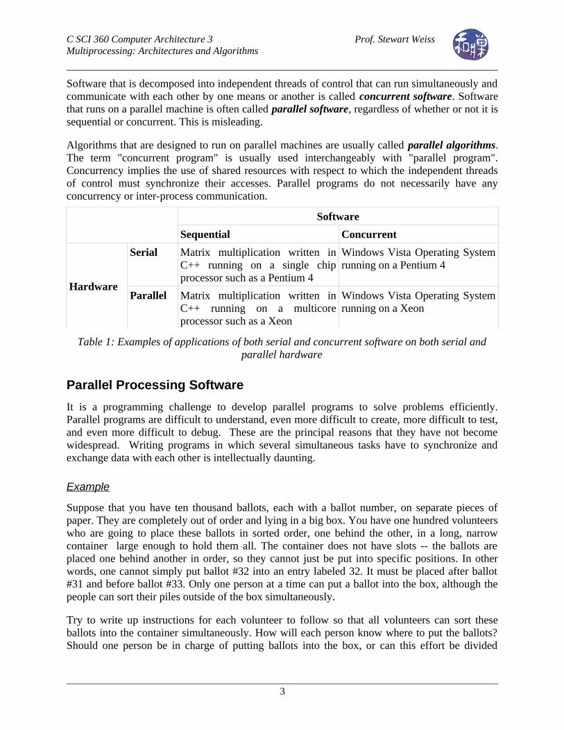
Software that is decomposed into independent threads of control that can run simultaneously and communicate with each other by one means or another is called concurrent software. Software that runs on a parallel machine is often called parallel software, regardless of whether or not it is sequential or concurrent. This is misleading.

Algorithms that are designed to run on parallel machines are usually called parallel algorithms. The term "concurrent program" is usually used interchangeably with "parallel program". Concurrency implies the use of shared resources with respect to which the independent threads of control must synchronize their accesses. Parallel programs do not necessarily have any concurrency or inter-process communication.

Software

Sequential Concurrent

Hardware

Serial Matrix multiplication written in C++ running on a single chip processor such as a Pentium 4

Windows Vista Operating System running on a Pentium 4

Parallel Matrix multiplication written in C++ running on a multicore processor such as a Xeon

Windows Vista Operating System running on a Xeon

Table 1: Examples of applications of both serial and concurrent software on both serial and parallel hardware

Parallel Processing Software

It is a programming challenge to develop parallel programs to solve problems efficiently. Parallel programs are difficult to understand, even more difficult to create, more difficult to test, and even more difficult to debug. These are the principal reasons that they have not become widespread. Writing programs in which several simultaneous tasks have to synchronize and exchange data with each other is intellectually daunting.

Example

Suppose that you have ten thousand ballots, each with a ballot number, on separate pieces of paper. They are completely out of order and lying in a big box. You have one hundred volunteers who are going to place these ballots in sorted order, one behind the other, in a long, narrow container large enough to hold them all. The container does not have slots -- the ballots are placed one behind another in order, so they cannot just be put into specific positions. In other words, one cannot simply put ballot #32 into an entry labeled 32. It must be placed after ballot #31 and before ballot #33. Only one person at a time can put a ballot into the box, although the people can sort their piles outside of the box simultaneously.

Try to write up instructions for each volunteer to follow so that all volunteers can sort these ballots into the container simultaneously. How will each person know where to put the ballots? Should one person be in charge of putting ballots into the box, or can this effort be divided

3


amongst the team? How will you prove that your algorithm is correct? Is it the best possible in terms of time? How can you prove it if it is?□

This exercise, which in itself is challenging, is just the tip of a large iceberg of challenges. Even when parallel programs are written, they do not necessarily take full advantage of the parallelism inherent in the hardware. And if all of this isn't discouraging enough, as the number of processors increases, there is no guarantee that the performance gain will match the increase in the number of processors. This limitation is a consequence of Amdahl's Law.

Amdahl's Law

Definition. The speedup of a parallel algorithm running on p processors is the running time of the fastest known serial algorithm running on a single processor of a p-processor computer divided by the running time of the parallel algorithm running on the same p-processor computer using all p processors.

For example, if a particular parallel algorithm takes 10 seconds running on a computer using all of its 20 processors, and the fastest known serial algorithm that solves this same problem takes 150 seconds when run on one of these processors, the speedup of the algorithm is 150/10 = 15.

Definition. The efficiency of a parallel algorithm running on p processors is the speed-up of the algorithm divided by the number of processors, p.

In the preceding example, the efficiency of the algorithm is 15/20 = 0.75, because it had a speedup of 15 and it used 20 processors to achieve it. Efficiency is always a number between 0 and 1.0.

Efficiency is a measure of how much a parallel algorithm takes advantage of the parallelism of the problem, as well as how well it utilizes the processors to decrease running time. For example, if a particular parallel algorithm has a speedup of 0.5p with p processors, then its efficiency is 0.5.

Gene Amdahl is a computer scientist who, among his many other accomplishments, formulated a law that puts limits on just how much speedup is possible for any given problem. It is called Amdahl's Law:

Let f be the fraction of operations in a computation that must be performed sequentially, where 0 ≤ f ≤ 1. The maximum speedup Smax(p) achievable by a parallel computer with p processors for this computation is

Smax(p) = 1/( f + (1-f)/p )

Notice that, as p approaches infinity, the maximum speedup approaches 1/f.

Most problems have input and output, for example. These are usually sequential operations, as the media they access are linear in nature.

4


Example 1

Twenty percent of the instructions in a particular parallel algorithm are inherently sequential. An implementation of it is run on a parallel computer with 20 processors. What is the maximum possible speed-up? What is the maximum possible efficiency? Do the same with p = 100.

Solution.

In this case, f = 0.2 and p = 20, so the maximum speed-up is 1/(0.2 + 0.8/20) = 1/0.24 = 4.17. The maximum efficiency would be 4.17/20 = 0.2085. When p = 100, the maximum speedup is 1/(0.2 + 0.8/100) = 1/0.208 = 4.808. The maximum efficiency would be 4.808/100 = 0.048.

Exercise

The maximum possible speedup in the preceding problem cannot exceed 5.0. An inverse problem is to ask how many processors would be needed to obtain a speedup of 4.9? For this many processors, what is the efficiency?

Example 2

An algorithm must compute the sum of two 1000 by 1000 matrices, after which it must print the diagonal elements of the resulting sum matrix. Since printing is inherently a serial operation and there are 1000 diagonal elements, the printing requires 1000 = 103 sequential operations. The sum of two n by n matrices, on the other hand, requires O(n2) operations using a brute force sequential algorithm. Thus, the summation would require 106 operations. These operations are independent and could be performed completely in parallel if we had 106 processors ( ignoring an issue called communication overhead, which we will discuss elsewhere.) With one processor, the algorithm requires 106 + 103 sequential operations, of which 103 are inherently sequential. What is the maximum speed-up for a parallel computer with 100 processors. What about for 1000 processors?

Solution.

In this case, f = and p = 100, so the maximum speedup with 100 processors is .With 1000 processors it is .Even though we increased the number of processors by a factor of 10, from 100 to 1000, the speedup increased by a factor of 5.5, roughly, from 90.99 to 500.25.

Example 3

What if we increase the matrix size to 10,000 in Example 2? What will the speed-up be with 100 and 1000 processors?

Solution.

5


In this case the sequential part takes 104 steps and the parallel part, 108 steps. Thus, f = 104 / (104 + 108 ) = 0.0001. With p = 100, the maximum speedup with 100 processors is 1/(0.0001 + 0.9999/100) = 1/0.010099 = 99.01.

With 1000 processors it is 1/(0.0001 + 0.9999/1000) = 1/0.0010999 = 909.17.In this case, when we increase the number of processors from 100 to 1000, the increase in speedup is roughly 9.2, from 99 to 909.

So with the larger size matrix, the speedup is much greater for the machine with more processors. In fact, the speedup increase is almost equal to the increase in the number of processors.

The Amdahl Effect

The preceding two examples show an interesting phenomenon. In each case, as the size of the problem was increased, the fraction of the computation that was serial became smaller, which in turn meant that the maximum speedup possible for that problem increased. For many types of problems, as the problem size increases, the fraction of operations that are inherently sequential decreases2. In the case of the matrix summation problem for a 10N by 10N the fraction of inherently sequential operations is approximately 10-N, so the fraction decreases exponentially. Amdahl's law puts an upper bound on potential speed-up, Smax. based upon this fraction. Therefore, as problem size increases for these types of problems, for a fixed number of processors, the maximum possible speed-up increases. This is an example of the Amdahl effect. The Amdahl effect is that, as problem size increases, the fraction of sequential operations in a problem may decrease, and hence the speed-up increases for a fixed number of processors. One way to see this is that small instances of problems do not enjoy the speedup on large parallel machines as well as large instances do.

Since parallel machines are often created not to decrease running time of a fixed size problem, but to increase the size of the problem that can be solved in a fixed amount of time, the Amdahl effect shows that this can often be accomplished.

Scaling

The preceding examples also showed that getting good speedup while keeping the problem size fixed and increasing the number of processors is harder than getting good speedup by increasing problem size while the number of processors remains fixed. What about increasing problem size and increasing the number of processors? Is it possible to keep the same level of efficiency as we increase both?

Let us use the term parallel system to mean a particular parallel algorithm running on a particular parallel computer system. We can informally define the scalability of a parallel system by the way in which its efficiency changes as the problem size and the size of the parallel system

2 Although we have not yet discussed this, the fraction of the execution time in a parallel program in which the independent processes communicate with each other also tends to decrease in many cases as problem size increases.

6


increase. (A precise definition of the scalability of a parallel system is outside of the scope of this course.)

We explain the concept informally. Suppose that a problem has size n. Let the memory required to solve a problem of size n be denoted M(n). The memory M' available in a parallel processor is proportional to p, the number of processors, because each processor has a fixed and constant amount of memory. As p increases, M' increases linearly with it. The problem size n cannot be increased more than the available memory M', i.e., M(n) <= M', because the space to solve the problem has to be available in physical memory. (Even with virtual memory, the physical memory imposes a limit on how big the problem can be.) Therefore, the size of the problem that can be solved as the number of processors increases depends on the function M(n). For example, if the amount of memory needed to solve a problem of size n is O(n2), then the number of processors would have to grow quadratically to accommodate the larger problem size in the limit.

The scalability of the parallel system, i.e., its ability to remain efficient as the number of processors is increased, depends on the function M(n), as well as on other factors which include the inherently sequential fraction of the computation and the communication overhead. The exact mathematical relationship is known as the isoefficiency metric. We do not cover it in this course.

Load Balancing

Load balancing refers to the distribution of the workload to the processors in the multiprocessor. The preceding examples assumed that the workload was always uniformly distributed. This is not always possible. When the load is imbalanced, the speed-up may not be as great.

Example

Suppose the problem is to perform two sums: a matrix sum of two 100 by 100 matrices, followed by computation of the trace of the result matrix, which is the sum of its diagonal elements. Suppose that an addition takes t time steps. The matrix addition takes 10000t steps sequentially, and the sum of the diagonal elements, 100t steps (actually 99t), so the optimal sequential algorithm takes 10100t steps.

Suppose now that the problem is solved on a machine with 100 processors. Suppose the problem is distributed by giving each processor an equal size piece of the matrix summation, after which one of them will perform the addition of the 100 diagonal elements sequentially3, i.e., in 100t steps. The matrix sum will take 10000t/100 = 100t steps followed by the scalar sum, another 100t steps, so the total time is 200t. The speedup is therefore 10100t/200t = 50.5.

Suppose one processor does 2% of the matrix summation work and the remaining processors do 98% of the work. Then the processor that does 2% of the 10000 additions, does 0.02*10000 = 200 additions, which implies that it takes 200t steps. The remaining 99 processors divide the 9800 additions among themselves as evenly as possible, but it should be clear that the one with 200 additions takes the longest, so the total amount of time to do the matrix addition is 200t and

3 It is possible to distribute it, but the gain will be negligible.

7


the scalar addition remains at 100t. Assume the scalar addition is performed on this same processor. The total time is now 300t, and the speedup in this case is 10100t/300t = 33.7. The speedup dropped from 50.5 to 33.7.

If one processor gets 5% of the load, the speedup is even worse. In this case, one processor does 500 additions while the remaining 99 do 9500. Suppose we shift the diagonal summation to one of the other processors, so that it can be done while the one with the larger load works. The total time is 500t+100t, and the speedup is 10100t/600t = 16.83.

This shows how an imbalanced workload can reduce the speedup significantly.

Type of Multiprocessors

Early Development

Parallelism has existed in computers for many decades, at various levels of design. For example, bit-parallel memory has been around since the early 1970s, and simultaneous I/O processing (using channels) has been used since the 1960s. Other forms of parallelism include bit-parallel arithmetic in the Arithmetic-Logic Unit (ALU), instruction look-ahead in the Control Unit, direct memory access (DMA), and some other less well-known techniques such as data pipe-lining and instruction pipe lining.

By a parallel computer, though, we mean something quite different: a machine with parallelism at a much higher level, such as one containing multiple CPUs. This level of parallelism only began to take hold in the commercial market in the last thirty years, mostly because microprocessor technology advances such as Very Large Scale Integration (VLSI) that took place in the late 1970's made it possible to build parallel computers much more economically, and increases in performance of microprocessor-based parallel machines outpaced those of mainframes and supercomputers. This does not mean they perform better than all such machines, but only that the rate of increase has been greater. Machines such as the Intel Paragon XP/S™ and the Thinking Machines CM-5™ (now an orphan) could outperform super computers such as the Cray Y/MP™.

In the 1980's companies such as Intel, Bolt, Berenek, and Newman (BBN), and Thinking Machines Corporation developed and sold parallel computers with different architectures. By the 1990's, many of the leading computer makers were selling parallel computers as well. But a great influence on the parallel computer market was a strategy adopted at NASA's Goddard Space Center, where, in 1994, they built a computer out of off-the-shelf hardware and free software, which they named Beowulf. Beowulf ran Linux on 16 Intel DX4 processors connected by Ethernet links. This strategy of using commodity hardware took hold.

Vector Processors and Processor Arrays

There are two essentially different models of parallel computers: vector processors and multiprocessors. A vector processor, is simply a machine that has an instruction that can operate on a vector. A pipelined vector processor is a vector processor that can issue a vector instruction that operates on all of the elements of the vector in parallel by sending those

8


elements through a highly pipelined functional unit with a fast clock. A processor array is a vector processor that achieves the parallelism by having a collection of identical, synchronized processing elements (PE), each of which executes the same instruction on different data, which are controlled by a single control unit. Every PE has a unique identifier, its processor id, which can be used during the computation. The control unit, which might be a full-fledged CPU, broadcasts the instruction to be executed to the processing elements, which execute it on data from a memory that is usually local to each, and can store the result in their local memories, or can return global results back to the CPU. A global result line is usually a separate, parallel bus that allows each PE to transmit values back to the CPU to be combined by a parallel, global operation, such as a logical-and or a logical-or, depending upon the hardware support in the CPU.

Because all PEs execute the same instruction at the same time, this type of architecture is suited to problems with data parallelism. Data parallelism is a type of parallelism that is characterized by the ability to perform the same operation on different data simultaneously. For example, a loop of the form

9

Figure 1: Processor array architecture.


for i = 0 to N-1 do a[i] = a[i] + 1;

has data parallelism because the updates to the distinct array elements a[i] are independent of each other and may be performed in parallel, whereas the loop

for i = 1 to N-1 do a[i] = a[i-1] + 1;

has no data parallelism because the update to a[i] cannot be performed until the update to a[i-1]. If the value of N is smaller than the number of processing elements, the entire loop takes the same amount of time as a single processor takes to perform the increment on a scalar variable. If the value of N is larger, then the work has to be distributed to the PEs so that they each update the values of several array elements. This may be handled by the hardware, by a runtime library, or by the programmer, depending on the particular architecture and software.

Data parallelism exists in many application areas, including all of the grand challenge problems mentioned earlier and most scientific problems in general. Commercial applications with a large degree of data parallelism also include image processing and high-end graphics.

Array processor hardware also has to handle what PEs do when they do not need to participate in a computation. For example, when N is smaller than the number of PEs in the above loop, then some PEs will have to be de-activated, or masked, during the computation. The PEs usually have the capability to mask themselves, which they would do conditionally depending on the value of their PE identifier.

The PEs are usually connected to each other through an interconnection network, which can take on many forms. Interconnection networks are covered later in this chapter.

Processor Array Disadvantages

• Not all problems are data parallel and therefore do not benefit from a processor array's architecture.

• When code has many branches and conditionally executed code, many PEs are inactive and the efficiency of the computation diminishes.

• Processor arrays are not suited to multiprogramming; only a single job can run well on them because to allow multiple programs to be scheduled on the PEs requires local memory partitioning as well as special hardware.

• They cannot be scaled down to smaller sizes and still be cost-efficient.

• They tend to be built with custom chips rather than off-the-shelf hardware and are therefore not competitive with processors containing many commodity processors.

10


Multiprocessors

All parallel computers are called multiprocessors in the textbook. The term multiprocessor can have a different meaning in other sources. Some people use the term to mean a particular type of parallel computer characterized by more autonomy among the separate processors. Here, we will use "multiprocessor" only to mean a computer with multiple CPUs.

Multiprocessors are divided into two types. One in which the processors share a physical address space is called a shared memory multiprocessor (SMP), and one in which the processors have private, non-shared address spaces, is called a private memory multiprocessor.

Shared Memory Multiprocessors

Shared memory multiprocessors are divided into two types: those in which all processors have equal access to the physical memory, called uniform memory access (UMA) multiprocessors, and those in which memory access is non-uniform, called non-uniform memory access (NUMA) multiprocessors. NUMA machines have physically separate memories, attached locally to each processor. It is much harder to write code for a NUMA multiprocessor than for a UMA multiprocessor. A UMA multiprocessor may also be called a symmetric multiprocessor, or SMP. Figure 2 shows a typical SMP design for a four-processor machine. Figure 3 shows a typical NUMA architecture. Note that in both cases, the processors have caches.

Figure 2 UMA or SMP design

Generally speaking, SMP architectures are appropriate for small servers and fast desktop systems. NUMA systems can scale to larger machines.

The interconnection between the processors in the NUMA case, or between the processors and memory in the UMA case, may be a simple bus, or a more complex interconnection network.

11


Buses are limiting because they are shared links; only one communication can be active at a time. Bus-based systems cannot have more than several dozen processors without degrading. Interconnection networks, such as butterfly or Omega networks, or crossbar networks, allow much larger numbers of processors, but are costlier to implement.

For both types of shared memory multiprocessors, the processors will be running tasks that share data. This data resides in the memory and therefore processes that share it must use some form of synchronization to prevent race conditions.

Figure 3 NUMA design

Clusters and Message-Passing Multiprocessors

Clusters are a form of private memory multiprocessor; they are individual processors with their own private memories attached by a network. They are message-passing systems. Because each processor has a private memory, no other processor can access its data directly. Instead, if a process on one processor needs data from another processor’s memory, it has to send a message requesting the data, hence the name. The hardware in a message passing system is much simpler, since the machines do not have to access a shared memory. They look like the NUMA design, except that the memories are not connected to the network. Message passing systems rely on the operating system's having support for sending and receiving messages. Typically there is support for some form of send() and receive() instructions.

Message-passing increases communication overhead and delays. A process that needs access to data in a remote memory must send the request for that data and wait for the data to be sent. Because of this, applications with little need for the exchange of data perform much better on

12


this type of parallel computer system than those that have large communication demands. In the past, many attempts were made to build high-performance, special-purpose computers with built-in message passing, but it turned out to be much less expensive to use off-the-shelf computers attached by standard network switches and cables. Such a system is called a cluster.

Clusters have much higher administrative overhead than a single machine, because there are multiple copies of the operating system and replicated hardware. This weakness led to the use of virtual machines in the clusters. The most efficient use of virtual machine technology puts a virtual machine on every physical node in such a way that each is managed by a single, centralized cluster manager. The cluster manager can migrate one machine to another in case of hardware failures.

Comparison of Memory Availability Between Cluster and UMA

Suppose that a single, UMA processor with 5 processors has 20GB of main memory and the operating system uses 1 GB of that memory. Suppose also that in a cluster of 5 computers, each has 4 GB and the operating system uses 1 GB in each. How much more memory is available in the UMA machine?

The shared memory machine has 19 GB of available memory. The cluster only has 5*3 GB = 15 GB of available memory. Thus, the shared memory machine has 4/15 more memory, or 27% more memory.

Flynn's Taxonomy

In the 1966, Michael Flynn4 proposed a categorization of parallel hardware based upon a classification scheme with two orthogonal parameters: the instruction stream and the data stream. In his taxonomy (naming scheme), a machine was classified by whether it has a single or multiple instruction streams, and whether it had single or multiple data streams. An instruction stream is a sequence of instructions that flow through a processor, and a data stream is a sequence of data items that are computed on by a processor. For example, the ordinary single-processor computer has a single instruction stream and a single data stream.

This scheme leads to four acronyms:

SISD single instruction, single data; i.e., a conventional uni-processorSIMD single instruction, multiple data; like MMX or SSE instructions in the x86 processor

series, processor arrays and pipelined vector processorsMISD multiple instruction, single data; very rare but one example is the U.S. Space Shuttle

flight controllerMIMD multiple instruction, multiple data; SMPs, clusters. This is the most common

multiprocessor

4 Flynn, M., Some Computer Organizations and Their Effectiveness, IEEE Trans. Comput., Vol. C-21, pp. 948, 1972.

13


SIMD Multiprocessors

SIMD multiprocessors issue a single instruction that operates on multiple data items simultaneously. Vector processors are SIMD multiprocessors, which means that processor arrays and pipelined vector processors are also SIMD machines. The Cray X-MP and Thinking Machines CM-1 or CM-2 are examples of SIMD machines.. The CM-2 could execute the same instruction on an array of 64,000 data items simultaneously.

MIMD Multiprocessors

MIMD multiprocessors are more complex and expensive, and so the number of processors tends to be smaller than in SIMD machines. Today's multiprocessors are found on desktops, with anywhere from 2 to 16 processors. Larger systems are still being manufactured, but they are expensive machines and thus have a limited market.

SPMD Programming

In addition to the above four classifications, people have used the acronym SPMD, single program, multiple data stream, to describe a process architecture, typically run on multicomputers with tightly-coupled architectures and either private memories or shared memories, in which the same program is run by identical processes on separate processors, either accessing a shared memory or private memories.

Multiprocessor Network Topologies

Networks are used to connect processors to processors, processors to memories and processor-memory nodes to each other. The way that these entities are connected to each other has a significant effect on the cost, applicability, scalability, reliability, and performance of the parallel computer. In general, the things that are connected to each other will be called nodes, whether they are processors, memories, or processor-memory elements. The set of connections between nodes is called an interconnection network.

An interconnection network may be classified as shared or switched. A shared network can have at most one message on it at any time. A bus is a shared network, as is Ethernet. In contrast, a switched network allows point-to-point messages among pairs of nodes and therefore supports the transfer of multiple concurrent messages.

Interconnection networks may also be classified as static or dynamic. A network is static if communication links between pairs of processors are "permanent": they can only be changed by physically reconfiguring the network. Static networks are usually constructed by point-to-point connections between processors. A network is dynamic if links are established by dynamically configuring switches to establish paths between processors and other processors or memory modules. There are three types of dynamic networks:

• crossbar switching networks, • single-stage networks, and

14


• multi-stage networks.

Buses have been classified as both static and dynamic. They are static in the sense that the physical communication links are permanent and fixed, if one ignores the ability to dynamically add devices to them. They are dynamic if devices can attach and detach themselves from the bus dynamically. Some authors claim that they are dynamic because the logical links change dynamically on the bus, but this is not consistent with the definition of static given above.

Static networks are usually used in highly parallel multiprocessors to connect processors to each other, whereas dynamic networks are usually used in multiprocessors to connect processors to memory nodes or other processors. Figure 4 is one way to classify the various types of interconnection networks.

In the figure, static networks are classified as either regular or irregular. This has to do with their topologies, which we will discuss below. Regular static networks can have shared or dedicated paths. Most of the static networks we examine have dedicated paths.

15

Figure 4: Taxonomy of interconnection networks


In mathematics, a topology is a set together with an adjacency relation on the set. Topologies do not have to be finite sets for mathematicians, but for computer scientists, the practical applications of topologies are finite sets. If you have already learned about graphs, then you know about topologies. Your mental picture of a topology should be a "tinker-toy" – a set of nodes connected by edges. In topologies, distance does not exist; when distance exists, the topology becomes a metric space. A graph is the same thing as a finite topology.

Networks can be characterized by their topologies. For example, a bus is a single line segment to which each node is attached, whereas a ring is like a bus in which the ends of the line segment are attached to each other, forming a cycle. Buses and rings have bidirectional links.

Although buses and rings are similar from a topological point of view, they are very different in their performance. In a bus, there is only a single link, and only one message at a time can be in

the network; it is a shared link. Each host checks to see if the message is addressed to it, and if not it ignores it. In contrast, in a ring, each host is attached to the network via a switch, and these switches act to separate the links. Thus, if there are n hosts, there are n links, and there can be n simultaneous messages on the network. Messages hop from one switch to another until they arrive at their destination address. These are just two very simple topologies. There are other, more complex topologies with interesting properties..

Network Performance Metrics

Network costs in general include the number of switches, the number of links per switch that connect to the network, the number of bits per link, and the lengths of the links. Network performance may be measured by

• latency to send and receive a message when the network is unloaded• throughput as measured by the number of messages per unit time• delays caused by contention for portions of the network that are highly shared

16

Figure 5: Bus topology

Figure 6: Ring topology


For each of these metrics, both the mean and the standard deviation are important, as high standard deviation implies less predictability. Another important factor is fault tolerance, the degree to which the network will remain functional when some part of it fails.

There are various other metrics that can be used to evaluate the performance of networks. One popular one is the total network bandwidth, which is the bandwidth of each link multiplied by the number of links. This represents the total number of messages that can be en route at any given instant of time. Network bandwidth usually refers to the peak bandwidth, but it can also mean the bandwidth of a single link. It is an ambiguous term. Bisection bandwidth, is informally, the sum of the bandwidths of the links that sever the network into two equal halves. It will be defined more precisely below.

Network Topology Evaluation Criteria

A network will be viewed as a graph. The edges might be directed or undirected, depending upon the particular design. Unless otherwise stated, the edges are undirected. By the distance between a pair of nodes, we mean the least number of edges that must be traversed to get from one node to the other. For example, in Figure 7, the distance between nodes 1 and 5 is 2, and the distance between nodes 4 and 6 is 4.

Figure 7 A network topology

Diameter. The diameter of a network is the largest distance between any pair of nodes in the network. The diameter of the network in Figure 7 is 4, since the distance between nodes 4 and 6 is 4, and there is no pair of nodes whose distance is 5. Diameter is important because if an arbitrary pair of processors might communicate, then the diameter determines a lower bound on the communication time. (Note that it is a lower bound and not an upper bound; if a particular algorithm requires, for example, that all pairs of nodes send each other data before the next step of a computation, then the diameter determines how much time will elapse before that step can begin.)

Bisection width. The bisection width (not the bisection bandwidth) is the smallest number of edges that must be deleted to severe the set of nodes into two sets of equal size, or size differing by at most one node. In Figure 7, edges (2,6), (2,5), (3,5), and (3,4) can be deleted to split the set of nodes into two sets {1,2,3} and {4,5,6}. Thus, 4 edges are removed to split the node set. Is

17

1

2

6

3

4

5


the bisection width 4? No. A smaller edge set that also splits the node set is {(1,3), (2,5)}. This splits the nodes into sets {1,2,6} and {3,4,5}. The bisection width of this network is 2. Bisection width is important because it can determine the total communication time. Low bisection width is bad, and high is good. Consider the extreme case, in which a network can be split by removing one edge. This means that all data that flows from one half to the other must pass through this edge. This edge is a bottleneck through which all data must pass sequentially, like a one-lane bridge in the middle of a four-lane highway. In contrast, if the bisection width is high, then many edges must be removed to split the node set. This means that there are many paths from one side of the set to the other, and data can flow in a high degree of parallelism from any one half of the nodes to the other.

Bisection bandwidth. This is the sum of the bandwidths of the links that must be removed to bisect the graph, as described above. If we assume that the number of messages per link is uniform and constant, then we can equate the bisection bandwidth and the bisection width, since we can take 1 to be the number of messages per link.

Maximum edges per node. The maximum number of edges per node can affect how well the network scales as the number of processors increases, because of physical limitations on how the network is constructed. In the network of Figure 7, the maximum number of edges per node is 3 (nodes 2 and 3 each have 3 incident edges.) For some networks, the number of edges per node is a constant independent of network size. This is good, because the physical design need not change to accommodate the increase in number of processors. In contrast, suppose that the number of edges increases with the number of processors. This means that as the network gets larger, more connections need to be made to each processor. Given that processors have a fixed pin-out, this implies that the connections between processors must be implemented by a complex fan-out of the wires, a very expensive and potentially slow mechanism.

Maximum edge length. Maximum edge length is important because the communication time is a function of how long the signals must travel. It is best if the network can be laid out in three-dimensional space so that the maximum edge length is a constant, independent of network size. If not, and the edge length increases with the number of processors, then communication time increases as the network grows. This implies that expanding the network to accommodate more processors can slow down communication time. In the network in Figure 7, the nodes can be laid out with constant edge length.

Static Topologies

There are many different network topologies. Some have been proposed but never realized. Others have found their way into commercial parallel computers. We will look at the most viable and the most interesting topologies.

Fully-Connected Network

In a fully-connected network, every node is connected to every other node, as in Figure 8. If there are n nodes, there will be n(n-1)/2 links. Suppose n is even. Then there are n/2 even numbered nodes and n/2 odd numbered nodes. If we remove every edge that connect an even node to an odd node, then the even nodes will form a fully-connected network and so will the odd nodes, but the two sets will be disjoint. There are (n/2) edges from each even node to every

18


odd node, so there are (n/2)2 edges that connect these two sets. Not removing any one of them fails to disconnect the two sets, so this is the minimum number. Therefore, the bisection width (and bandwidth) is (n/2)2. The diameter is 1, since there is a direct link to any node from every node. The maximum edges per node is proportional to n, so this network does not scale well. Lastly, the maximum edge length will increase as the network grows, under the assumption that nodes take fixed amount of space. (Think of the nodes as lying on the surface of a sphere, and the edges as chords connecting them.)

Figure 8: Fully-connected network with 8 nodes.

Mesh networks

In a mesh network, nodes are arranged in a q-dimensional lattice. A 2-dimensional lattice with 36 nodes is illustrated in Figure 9. In general, there are k2 nodes in a 2-dimensional mesh. A 3-dimensional lattice is the logical extension of a 2-dimensional one. It is not hard to imagine a 3-dimensional lattice. It consists of the lattice points in a 3-dimensional grid, with edges connecting adjacent points. A 3-dimensional mesh must have k3 nodes, for k = 1,2,3,...., like three-dimensional graph paper. While we cannot visually depict q-dimensional mesh networks when q > 3, we can describe their properties. A q-dimensional mesh network has kq nodes. k is the number of nodes in a single dimension of the mesh. Henceforth we let q denote the dimension of the mesh, and d, the number of nodes in a single dimension.

Communication is allowed only between neighboring nodes. The neighbors of a node are the nodes to which it is directly connected. The interior nodes of a mesh are connected to 2q other processors. (In the 2d case, they are connected to 4 processors; in the 3d case, to 6.) Non-interior nodes have fewer neighbors, depending upon their exact position. For example, "corner" nodes are connected to q processors.

19


Figure 9 Two-dimensional mesh of size 36

We can evaluate the mesh network according to the criteria stated above. The diameter of a q-dimensional mesh network with kq nodes is q(k - 1). The first step in understanding this is realizing that the farthest distance between nodes is from one corner to the diagonally opposite one. A recursive argument should convince you that the diameter is correct. In a 2-dimensional lattice with k2 nodes, you have to travel (k - 1) edges along the bottom row, then (k - 1) edges along the extreme column to get to the opposite corner. Thus you travel 2(k - 1) edges. Suppose we have a mesh of dimension q - 1. By assumption its diameter is (q-1)(k - 1). A mesh of one higher dimension has (k - 1) copies of the (q - 1)-dimensional mesh, side by side. To get from one corner to the opposite one, you have to travel to the corner of the (q - 1)-dimensional mesh first. That requires crossing (q - 1)(k - 1) edges, by hypothesis. Then we have to get to the kth copy of the mesh in the new dimension. We have to cross (k - 1) more edges. Thus we travel a total of

(q - 1)(k - 1) + (k - 1) = q(k - 1)edges. The result is proved.

The diameter of a mesh increases as a linear function of the dimensionality of the mesh and the length of the side of the mesh; this can be a problem for many algorithms that require a lot of data movement, because data must be routed through many processors in the worst case.

If k is an even number, the bisection width of a q-dimensional mesh network with kq nodes is kq-1. Consider the 2d mesh of Figure 9. To split it into two halves, you can delete 6 = 61 edges. Imagine the 3d mesh with 216 nodes. To split it into two halves, you can delete the 36 = 62

vertical edges connecting the 36 nodes in the third and fourth planes. In general, one can delete the edges that connect adjacent copies of the (q-1)-dimensional lattices in the middle of the q-dimensional lattice. There are kq-1 such edges. This is a very high bisection width. One can

prove by an induction argument that the bisection width when k is odd is ∑0

q−1k i

.

20


The maximum number of edges per node in a mesh is fixed for each given q: it is always 2q. The maximum edge length is also a constant, independent of the mesh size, for two- and three-dimensional meshes. For higher dimensional meshes, it is not constant.

The two-dimensional mesh is a popular topology for processor arrays. It was used in the Goodyear Aerospace MPP™, the AMT DAP™, and the MasPar MP-1™. The Intel Paragon

XP/S™ multi-computer used a two-dimensional mesh to connect its processors.

An extension of a mesh is a torus. A torus, the 2-dimensional version of which is illustrated in Figure 10, is an extension of a mesh by the inclusion of edges between the exterior nodes in each row and those in each column. In higher dimensions, it includes edges between the exterior nodes in each dimension. It is called a torus because the surface that would be formed if it were wrapped around the nodes and edges with a thin film would be a mathematical torus, i.e., a doughnut.

Binary Tree Networks

In a binary tree network the 2k -1 nodes are arranged into a complete binary tree of depth k-1. (See Figure 11) Recall that the depth of a binary tree is the maximum number of edges from the root to a leaf node. Each interior node is connected to two children, and each node other than the root is connected to its parent. Thus the maximum number of edges per node is three. The diameter of a binary tree network with 2k -1 nodes is only 2(k - 1), because the longest path in the tree is any path from a leaf node up to the root and then down to a different leaf node. If we let n = 2k -1 then 2(k-1) is approximately 2log2 n; i.e., the diameter of a binary tree network with n nodes is a logarithmic function of network size, which is very low.

21

Figure 10: Torus network


The bisection width is low, which means it is poor. It is possible to split the tree into two sets differing by at most one node in size by deleting either edge incident to the root; the bisection width is one. Maximum edge length is an increasing function of the number of nodes, assuming that there is a lower bound on the physical size of each processor. As technology advances, the size of processors has diminished. It is reasonable to assume that there is a lower bound on that size, i.e., that they cannot shrink ad infinitum. If we try to lay out successively larger complete binary trees, the edge lengths must increase because the deepest layer of the tree determines the width of the tree and therefore the length of the edges between higher layers.

Figure 11 Binary tree network of depth 3 and size 15

Hypertree Networks (optional)

The problem with binary trees is their poor bisection width. Their advantage is their low diameter. A hypertree network is a modification of a binary tree with high bisection width but low diameter. The degree of a hypertree is the number of children per node. The degree of a hypertree must be a power of 2, i.e., 2, 4, 8, and so on, so we can have 2-ary, 4-ary, 8-ary 16-ary hypertrees etc. Unlike a binary tree, each node in a hypertree below the root level has two parents (just like people.) The best way to visualize a hypertree of degree k and depth d is to view it three dimensionally, using front and side views. In the frontal view, a hypertree of degree k and depth d looks like a k-ary tree of depth d, as shown in Figure 12. From the side, a hypertree looks like an upside down binary tree of depth d.

Figure 12 A 4-ary hypertree of depth 2 (front and side views)

22


Hypercube (Cube-Connected) Networks

A cube-connected network is a network with 2k nodes arranged as the vertices of a k-dimensional cube, also called a hypercube. A square with edge length d is a 2D hypercube, consisting of the 4=22 vertices (0,0), (0,d), (d,d), and (d,0). A cube with edge length d is a 3D hypercube, consisting of the 8=23 vertices (0,0,0), (0,0,d), (0,d,d), (0,d,0), (d,0,0), (d,0,d), (d,d,d), and (d,d,0). This topology can be generalized to higher dimensions if we do not try to associate a picture with it. For simplicity assume that d=1, i.e., that the edge length is 1. A hypercube with unit length is called a unit hypercube, or simply a hypercube. The 4D hypercube consists of the 16 vertices

Node Label(0,0,0,0) 0(0,0,0,1) 1(0,0,1,1) 3(0,0,1,0) 2(0,1,1,0) 6(0,1,1,1) 7(0,1,0,1) 5(0,1,0,0) 4(1,1,0,0) 12(1,1,0,1) 13(1,1,1,1) 15(1,1,1,0) 14(1,0,1,0) 10(1,0,1,1) 11(1,0,0,1) 9(1,0,0,0) 8

If we could draw things in four dimensions, this would look like a cube of unit length in four dimensions. Notice that the coordinates of the points can be thought of as 4-bit binary representations of integers. The numbers adjacent to the vertices in the column to the right are the corresponding numbers. The integer representation of a node is called its label.

Notice too that the sequence of bit strings above has the property that each string differs from the adjacent ones by a change of exactly one bit, considering the first string as following the last as if in a circular list. Two nodes are adjacent if their labels differ in exactly one bit position. Adjacent nodes are connected by edges. In a k-dimensional hypercube, each node is represented by k bits. Each of these bits can be inverted (0->1 or 1->0), so each node has exactly k incident edges. In the 4D hypercube, for example, each node has 4 neighbors.

While it is hard to visualize a k-dimensional hypercube as a cube in k dimensions, it is not hard to lay out its nodes in the plane. In Figure 13, a planar layout of the 4D hypercube is illustrated.

Notice that one can traverse all nodes in the hypercube by following the sequence of labels in the above table.

23


Figure 13: A four-dimensional hypercube.

The diameter of a k-dimensional hypercube is k. To see this, observe that a given integer represented with k bits can be transformed to any other k-bit integer by changing at most k bits, one bit at a time. This corresponds to a walk across k edges in a hypercube from the first to the second label. The bisection width of a k-dimensional hypercube is 2k-1. One way to see this is to realize that all nodes can be thought of as lying in one of two planes: the nodes with first bit = 0 are in one plane, and those with first bit = 1 are in the other. To split the network into two sets of nodes, one in each plane, one has to delete the edges connecting the two planes. Every node in the 0-plane is attached to exactly one node in the 1-plane by one edge. There are 2k-1 such pairs of nodes, and hence 2k-1 edges. No smaller set of edges can be cut to split the node set.

The bisection width is very high (one half the number of nodes), and the diameter is low. This makes the hypercube an attractive organization. Its primary drawbacks are that (1) the number of edges per node, k, is a (logarithmic) function of network size, making it difficult to scale up, and the maximum edge length increases as network size increases. This is also a serious impediment to using it for massively parallel designs.

In spite of these drawbacks, the hypercube was the most popular processor organization for first- and second-generation multicomputers, and it is still used today in nCUBE machines. The processing element clusters on the CM-200 processor array are connected in a hypercube.

Crossbar Switching Networks

A crossbar matrix is an example of a dynamic network because the switches can be changed dynamically. Given p processors and m memory modules, a crossbar matrix consists of a rectangular grid of p*m switches, as illustrated in Figure 14. In the figure, each Mi is a memory module and each Pj is a processor.

Switches are placed at the intersections of the horizontal and vertical lines in the matrix. Although the crossbar matrix in Figure 14 connects processors to memory modules, in general a crossbar connects input lines, which are the horizontal lines in the matrix, with output lines, which are the vertical lines; the inputs and outputs do not have to connect to processors and

24

0

2

3

1

11

9

8

10

5

7

6

4 12

13

14

15


memories in general. Figure 15 shows how this same crossbar matrix could be used to connect the processors back to themselves.

25

Figure 14: Crossbar network (4 by 4)

M1 M2 M3 M4

P1

P2

P3

P4

Figure 15: Crossbar switch used to connect processors to processors


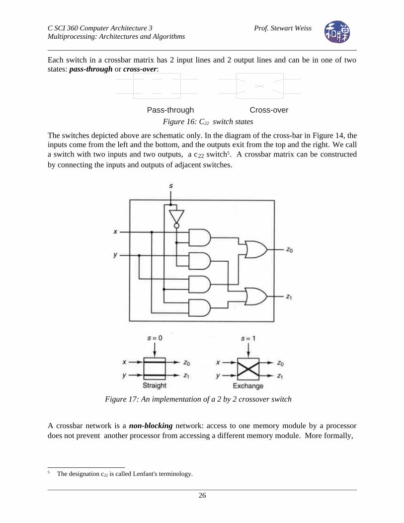
Each switch in a crossbar matrix has 2 input lines and 2 output lines and can be in one of two states: pass-through or cross-over:

The switches depicted above are schematic only. In the diagram of the cross-bar in Figure 14, the inputs come from the left and the bottom, and the outputs exit from the top and the right. We call a switch with two inputs and two outputs, a c22 switch5. A crossbar matrix can be constructed by connecting the inputs and outputs of adjacent switches.

A crossbar network is a non-blocking network: access to one memory module by a processor does not prevent another processor from accessing a different memory module. More formally,

5 The designation c22 is called Lenfant's terminology.

26

Figure 16: C22 switch states

Cross-overPass-through

Figure 17: An implementation of a 2 by 2 crossover switch


Definition. A network is non-blocking if, for all sets of connections that can be established, all inactive input lines have access to all inactive output lines.

In Figure 18, there are two inputs connected to two different outputs: P3 is connected to M2 while P2 is connected to M4.

It is assumed that p <= m, since otherwise there could be processors without memory modules to access. The disadvantage of using crossbar networks is that to connect p processors to m memory modules requires Ω(pm) switches, or to interconnect p processors as in Figure 15, Ω(p2) switches. This makes them costly to construct. Crossbars are used in the Cray Y-MP and Fujitsu VPP 500. The VPP uses a crossbar of size 224 x 224.

Multistage Networks

Certain network topologies are more suitable to be used in multistage networks. In a multistage network, instead of having a processor at each node, there is a switch at the node. The switches are less expensive and smaller and can be packed very densely. They are called multistage because a message travels from one switch to another in stages. Two common multistage networks are butterfly networks and omega networks.

Multistage networks are a compromise between buses and crossbars in terms of cost and performance -- they are less costly (Ω(p log p) switches versus Ω(pm) switches) than crossbars and slower than them, but faster than buses and more costly than them. A network with p processors will usually have log p stages. Messages travel from a processor to a memory module or other processor in successive stages across the network. These networks are generally blocking networks; two processors attempting to access different memory modules may not both be able to do so. This will be evident soon.

27

Figure 18: Crossbar matrix showing two simultaneous connections

M1 M2 M3 M4

P1

P2

P3

P4


Butterfly Networks

A butterfly network represents a very different approach than the preceding ones. Butterfly networks are often used as multistage networks. A butterfly network consists of (k + 1)2k nodes arranged in k + 1 ranks, each containing n = 2k nodes. The ranks are labeled 0 through k. Sometimes ranks 0 and k are combined. Figure 19 depicts a butterfly network with 8 processor nodes. In the figure, the ranks are vertical. The rank 0 nodes would be connected to processors, and the rank 3 nodes could be connected either to processor nodes or to memory nodes, if the network were being used to implement a SMP machine. In a butterfly network, there is a path of length k from any node in rank 0 to any node in rank k+1. Since k is log n +1, where n is the number of inputs, this is a log n stage network.

Each switch in a butterfly network has two inputs and two outputs. The inputs come from two nodes in the preceding rank, and the outputs, to two nodes in the following rank. Which nodes depends upon the switch's position in the network.

An easy way to understand the butterfly network is as a recursive network. The base case is a 2 by 2 network, one with 2 inputs and 2 outputs. This is when k=1:

Suppose that we have constructed a butterfly for degree k=n. A butterfly of degree n has 2n

inputs and 2n outputs. To construct one for degree k=n+1, we replicate the butterfly of degree n

28

Figure 19: A butterfly network with 32 nodes.


and place tit under the original. This will have 2n+1 inputs and 2n+1 outputs. If we think of the inputs as being written in binary, then the original inputs had n bits and the new inputs will have n+1 bits. The way the new inputs are connected to the butterfly of degree n+1 is that the inputs whose low order n bits are the same are connected to the same inputs of the switches. In other words, input i and 2n + i are connected to the same switches; the outputs do not change. The construction for k=2 is illustrated below.

This can be stated mathematically as well. We will call the line of nodes perpendicular to a rank, a "chain". Let node[i,j] refer to the node in rank i and chain j, where 0 ≤ i ≤ k and 0 ≤ j < 2k. If i > 0 then node[i,j] is connected to node[i-1, j] and node[i-1,m], where m is the integer obtained by inverting the ith most significant bit in the binary representation of j. It is assumed that the binary representation has k bits. For example, in the butterfly network with k = 3, as shown in the figure, there are 4 ranks and 8 chains. Node[3,5] would be connected to node[2,5] and node[2,4] because inverting the 3rd most significant bit of 5 (101) yields (100), which is 4. Note that by symmetry node[i,j] is also connected to node[i+1,j] if i < k+1, and if node[i,j] is connected to node[i-1,m] then node[i,m] is connected to node[i-1,j] because j is the integer obtained by inverting the ith most significant bit in the binary representation of m. For example, node[3,5] is also connected to node[4,5] and node[3,4] is connected to node[2,5]. This symmetry results in a "butterfly" pattern. For small values of i, the most significant bits are inverted. This means that the nodes are connected to chains that are very far away. As i increases, i.e., as we move to nodes of higher rank in the network, less significant bits are inverted, so the connections are shorter. The nodes in the highest rank are connected to nodes in the adjacent one..

This last observation shows that the maximum edge length increases as the size of the network increases, since chains get further apart. The number of edges per node is constant though; it is at most four, independent of network size.

The diameter of a butterfly network with (k + 1)2k nodes is k, if the output nods are connected back to the input nodes on the left side of the network. If not, and the network is two-sided, then the diameter is 2k. It can be shown that the nodes that are farthest apart are the first and last nodes in rank 0. To travel from one to the other requires traveling up the first chain to the last node, and then along a chain of diagonal edges to the first row again. This is a total of 2k edges.

29

Figure 20: Butterfly network of degree 2.


The bisection width is 2k. To split the network requires deleting all edges that cross between chains 2k-1 -1 and 2k-1.Only the nodes in row 1 have connections that cross this divide, because only inverting the most significant bit results in a number that is on the other side of this dividing line. There are 2k nodes in row 1, and one edge from each to a node on the other side of the line.

Routing in the butterfly network is easy to understand from the recursive definition given above. In the base case, a network of degree 1, if the output is the "0" output, the message travels to the top output, and if it is the "1" or bottom output, it travels down to the bottom of the switch. This idea applies recursively. Suppose that we want to route the message from an input switch to an output switch in the degree n+1 network. If the output switch is in the lower half, i.e., the copy that was duplicated from the degree n network and placed below the original, then the first step in the route is to travel to the copy of the input switch in the bottom copy, not the top copy, otherwise to the top copy. This procedure is applied again recursively at the next switch. If the output is in the bottom copy of this degree n network, then the next step is to route the message downward, otherwise to the top copy. This shows that the route is unique.

The more mathematical description of the route is as follows. If you write the output switch as a binary number, then the route at rank i is determined by the value of the i th most significant bit. If that bit is 0, the 0 output of the switch is taken, otherwise the 1 output of the switch is taken.

The butterfly network is a blocking network; a connection between an input and an output can prevent a different connection from being established between a different input and output even though neither is in use. For example, a connection from input 000 to output 111 prevents a message from being routed from input 100 to output 100, because the first switch is in a cross-over state. If the network is two-sided, meaning that messages can be sent in the reverse direction as well as the forward direction, then soem of the blocking can be avoided by allowing messages to be sent in multiple passes. In other words, a message may be sent to an output and then sent backwards to a different switch to take a path to the given destination.

One last observation: return to the picture in Figure 19 of a butterfly network. Imagine taking each horizontal row and enclosing it in a single box. Call each box a node. There are now 2k

nodes. Any edge that was incident to any node within the box is now considered incident to the new node (i.e., the box). The resulting network contains 2k nodes connected in a k-dimensional hypercube. This is the relationship between butterfly and hypercube networks. So for example, the route in the degree 3 network in Figure 19 above, to go from input 011 to output 110 would take the 1 output followed by the 1 output in the next rank and finally the 0 output in the third rank.

A butterfly network is used in the BBN TC2000 multiprocessor to route data from non-local memory to processors.

Omega Network

The omega network is very similar to the butterfly6. A three-stage omega network is illustrated in Figure 19. The only difference is in how the inputs and outputs of the switches are arranged.

6 In fact, by a simple permutation of the switches you can turn one into the other.

30


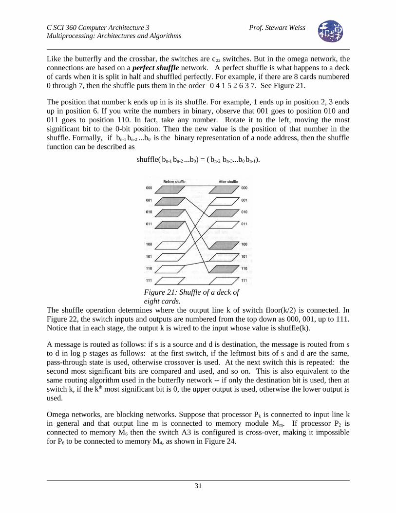
Like the butterfly and the crossbar, the switches are c22 switches. But in the omega network, the connections are based on a perfect shuffle network. A perfect shuffle is what happens to a deck of cards when it is split in half and shuffled perfectly. For example, if there are 8 cards numbered 0 through 7, then the shuffle puts them in the order 0 4 1 5 2 6 3 7. See Figure 21.

The position that number k ends up in is its shuffle. For example, 1 ends up in position 2, 3 ends up in position 6. If you write the numbers in binary, observe that 001 goes to position 010 and 011 goes to position 110. In fact, take any number. Rotate it to the left, moving the most significant bit to the 0-bit position. Then the new value is the position of that number in the shuffle. Formally, if bn-1 bn-2 ...b0 is the binary representation of a node address, then the shuffle function can be described as

shuffle( bn-1 bn-2 ...b0) = ( bn-2 bn-3...b0 bn-1).

The shuffle operation determines where the output line k of switch floor(k/2) is connected. In Figure 22, the switch inputs and outputs are numbered from the top down as 000, 001, up to 111. Notice that in each stage, the output k is wired to the input whose value is shuffle(k).

A message is routed as follows: if s is a source and d is destination, the message is routed from s to d in log p stages as follows: at the first switch, if the leftmost bits of s and d are the same, pass-through state is used, otherwise crossover is used. At the next switch this is repeated: the second most significant bits are compared and used, and so on. This is also equivalent to the same routing algorithm used in the butterfly network -- if only the destination bit is used, then at switch k, if the kth most significant bit is 0, the upper output is used, otherwise the lower output is used.

Omega networks, are blocking networks. Suppose that processor Pk is connected to input line k in general and that output line m is connected to memory module Mm. If processor P2 is connected to memory M6 then the switch A3 is configured is cross-over, making it impossible for P6 to be connected to memory M4, as shown in Figure 24.

31

Figure 21: Shuffle of a deck of eight cards.


Omega networks are often designed to be broadcast networks. In a broadcast network, the switches can be in any of four different states:

By setting selected switches to either of the two broadcast states, a single input can be sent to all outputs.

An omega network is used in the NYU Ultracomputer, a massively parallel machine with up to 4096 processors, to connect the processors to the memory banks. This omega network has the property that the switches have small buffers, enabling them to queue packets when a conflict occurs.

32

Figure 23: Four state C22 switch.

Figure 22: Three stage omega network (courtesy of Wikipedia)


Parallel Programming on Different ArchitecturesWe contrast the method of parallel programming on a shared memory architecture and a private-memory architecture.

Parallel Programming Example on a UMA Achitecture

A program that sums 100,000 numbers on a UMA multiprocessor with 100 processors. Idea: split the set of 100,000 numbers into 100 sets of 1000 numbers each. Give each processor a set to add, and then combine the sums. The numbers will reside in the shared memory; each processor will get the index of its first number: processor 0 gets 0 to 999, 1 gets 1000 to 1999, and so on. The processors execute an ordinary sequential loop. Let the processor id of the processor be denoted by pk. Each processor executes the same code, the addition loop of which is

sum[pk] = 0;for ( i = 1000*pk; i < 1000*(pk+1); i++ ) sum[pk] = sum[pk] + A[i];

Note that the variable pk has a different value in each processor. There will be 100 sums to add together, in the array sum[100]. With multiple processors, this can be done in time proportional to log2 (100) using something like a buddy system. Think of the set of 100 processors as being divided initially into two sets, the ones numbered 0 to 49, and the others. The lower numbered processors I will call the left-half, and the higher numbered ones, the right half. Each processor has a "buddy" which is the processor whose number differs from it by the value of an integer variable named half, which is initially 50.

1 half = 100;2 repeat3 synch(); // wait for all active processes to arrive here

33

Figure 24: Omega network with P2 connected to M6


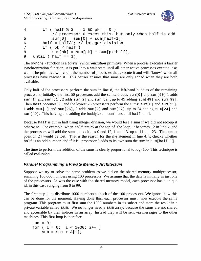
4 if ( half % 2 == 1 && pk == 0 ) // processor 0 execs this, but only when half is odd5 sum[0] = sum[0] + sum[half-1];6 half = half/2; // integer division7 if ( pk < half )8 sum[pk] = sum[pk] + sum[pk+half];9 until ( half == 1);

The synch() function is a barrier synchronization primitive. When a process executes a barrier synchronization function, it is put into a wait state until all other active processes execute it as well. The primitive will count the number of processes that execute it and will "know" when all processes have reached it. This barrier ensures that sums are only added when they are both available.

Only half of the processors perform the sum in line 8, the left-hand buddies of the remaining processors. Initially, the first 50 processors add the sums: 0 adds sum[0] and sum[50] 1 adds sum[1] and sum[51], 2 adds sum[2] and sum[52], up to 49 adding sum[49] and sum[99]. Then half becomes 50, and the lowest 25 processors perform the sums: sum[0] and sum[25], 1 adds sum[1] and sum[26], 2 adds sum[2] and sum[27], up to 24 adding sum[24] and sum[49]. This halving and adding the buddy's sum continues until half == 1.

Because half is cut in half using integer division, we would lose a sum if we did not recoup it otherwise. For example, when half == 25 at the top of the loop, it becomes 12 in line 7, and the processors will add the sums at positions 0 and 12, 1 and 13, up to 11 and 23. The sum at position 24 would be lost. That is the reason for the if-statement in line 4; it checks whether half is an odd number, and if it is, processor 0 adds to its own sum the sum in sum[half-1].

The time to perform the addition of the sums is clearly proportional to log2 100. This technique is called reduction.

Parallel Programming a Private Memory Architecture

Suppose we try to solve the same problem as we did on the shared memory multiprocessor, summing 100,000 numbers using 100 processors. We assume that the data is initially in just one of the processors. As was the case with the shared memory model, each processor has a unique id, in this case ranging from 0 to 99.

The first step is to distribute 1000 numbers to each of the 100 processors. We ignore how this can be done for the moment. Having done this, each processor must now execute the same program. This program must first sum the 1000 numbers in its subset and store the result in a private variable called sum. We no longer need a sum array, because the sums are not shared and accessible by their indices in an array. Instead they will be sent via messages to the other machines. This first loop is therefore

sum = 0;for ( i = 0; i < 1000; i++ ) sum = sum + A[i];

34


The next step is more complicated than the shared memory example. The sums must be exchanged by messages using the reduction technique. There is no need for barrier synchronization because the message-passing system acts as a means of synchronizing processes.

The two message-passing primitives are send() and receive(). These are not symmetric operations. The send operation has the form send(dest, message), which tries to send the message pointed to by message to the processor with id dest. This operation is non-blocking, meaning that it immediately returns and the process continues executing. The receive operation has the form receive(), which is a blocking operation, meaning that it is blocked until the message arrives. For those who have not had operating systems, "blocked" means that the process stops using the processor, and exists in a dormant state, waiting to be awakened or reactivated. Whether or not it remains in memory depends on the operating system and how long a wait is expected. When a message arrives, it returns the message as its return value. Notice that it does not specify the id of the process from which it expects the message. Any message that it receives satisfies the call.

In each iteration, the set of all processors is divided into two disjoint sets of senders and receivers. The upper set of indices are the senders and the lower half are the receivers. At the end of the iteration, the set of processors is halved, so some of the processes that were receivers before become senders. For example, initially, processors 0 through 49 are receivers and 50 through 99 are senders. The senders send their sums to their buddy receivers, and then they become dormant -- their work is done. When a receiver with an id between 25 and 49 receives its message, it performs an addition and then becomes a sender. The receivers whose ids are within the range 0 through 24 remain receivers in the next iteration.

In each stage, the processors are "buddied" using the same arithmetic as in the shared memory example -- for each k from 0 to 49, processors k and k+50 are buddies in round 1, then for each k from 0 to 24, k and k+25 are buddies, then in round 3, k and k+12, and so on, until ultimately in the last round, 0 and 1 are buddies.

When the number of nodes in the round is an odd number, what to do with the odd sum is solved in a different way than in the shared memory program. In that solution, processor 0 collected the sums of the processors that had no buddy. In this solution, the odd-numbered processor that has no buddy will act like a receiver and pretend to receive a sum from an imaginary buddy, but it will not receive anything. Then it will send its sum to its lower buddy when it becomes a sender. The code follows.

1 limit = half = 100;2 repeat3 half = (half+1)/2; 4 if (pk >= half && pk < limit) 5 send(pk-half, sum); 6 if (pk < limit/2)7 sum = sum + receive();8 limit = half;9 until ( half == 1);

35


This code is harder to understand than the shared memory code because there are two variables, half and limit. half is the dividing line between senders and receivers. In particular, in line 4, you can see that the processor whose id equals half is the lowest index sender, and that a processor whose id is limit or greater is out of the game completely -- it neither sends nor receives. To be a receiver, a processor has to have an id strictly less than limit/2, using integer division.

To illustrate, in iteration 1, processes 50 through 99 send in line 5 to their buddies from 0 to 49. None of the senders in this round satisfy the condition in line 6, so none can be receivers. (This is true in any round, because if pk > half, pk cannot be less than limit/2.) In round 1, processes 0 through 49 satisfy (pk < limit/2) so they each wait for the sum in line 7 from their buddies. In the next iteration, half = 25 and limit = 50. Processes 25 through 49 are senders and 0 through 24 are receivers. In the next iteration, half = 13 and limit = 25. Processes 13 through 24 are senders, and 0 through 11 are receivers. Note that, in this iteration, process k sends to process k-13, not k-12. So process 24 sends to process 11. Process 12 receives from no process. This is the sense in which it gets a zero. In the next iteration, half = 7 and limit = 13. Processes 7 through 12 are senders, and 0 through 5 are receivers. This is where process 12 gets to send its sum down the pike. This continues until all sums have accumulated in process 0's sum.

We ignored the issue of how the data is distributed among the processors initially. Although we could just have the first processor iteratively send to each processor one after the other, there are algorithms like the reduction algorithms that recursively split the data and send so that each processor takes part in the act of distributing the data. We will not discuss it here.

In spite of the fact that the software is more complicated, clusters are attractive because they are more scalable, more available, cheaper, and more energy efficient. That is why they continue to grow in popularity.

Review of Pipelining

Pipelining in a processor is an implementation technique in which multiple instruction sequences are overlapped in their execution. It is a way to take advantage of the independence of the hardware units to increase the throughput of the processor. If you ever learned about how a factory assembly line works, then you already know how pipelining works.

Some factory that makes widgets has a very long conveyor belt, perhaps one hundred meters long. Along the belt are twenty workstations where different parts are attached to a widget. A widget frame is placed at the start of the belt, and each time it reaches a new workstation, a machine there adds a new part to it. By the time it rolls off of the conveyor belt, after workstation #20, it is complete and ready to be inspected. Suppose that each step takes an equal amount of time, say 5 minutes. Then it takes 100 minutes to assemble a widget.

There are two ways to use this equipment. The not-particularly-smart way is to put a single widget on the conveyor belt, and when it reaches the end, put the next widget on. In this case the throughput is 1 widget per 100 minutes. However, since each workstation can do its task in 5

36


minutes, we can put the first widget on, wait 5 minutes, put the second on, wait 5 minutes, put the third on, and so on, so that the widgets are spaced 5 minutes apart in time, non-stop. Initially, it will take 100 minutes before the belt is fully loaded with widgets, but once it is, a widget is completed every 5 minutes, and the throughput is 20 widgets per 100 minutes. It still takes 100 minutes to assemble a single widget, but at any moment in time after the belt is fully loaded, 20 widgets are simultaneously under construction.

The first method of using the conveyor belt is the non-pipelined method. The second is the pipe-lined method. The speed-up of the pipe-lined method over the non-pipelined method is 20, since it completes 20 times as many widgets per unit time. Notice that we are measuring speed-up by comparing the throughput rather than "execution time" of each method. This makes sense because the throughput is a measure of the work done by the factory.

This idea applies to processors in a natural way. The conveyor belt is the data path. The stages are the different parts of the instruction cycle, e.g. fetch, register reads, execute (ALU), data

37

Figure 26: Pipelined processor with unequal stage lengths

Time 100 200 300 400 500 600 700 800 900100 200 300 400 500 600 700 800 900100 200 300 400 500 600 700 800 900

fetch ALU data accfetch ALU data accfetch reg ALU data acc

fetch ALU data accreg reg

reg

fetch ALU data accfetch ALU data accfetch reg ALU data acc


reg


Figure 25: Pipelined processor with uniform length stages

Time

fetch reg ALU data acc reg

100 200 300 400 500 600 700 800 900






100 200 300 400 500 600 700 800 900






100 200 300 400 500 600 700 800 900






access, and register write. Figure 25 illustrates a pipelined processor in which each instruction stage takes the same number of clock cycles.

If not all stages take the same amount of time in the processor, then the longest stage determines the stage time. For example, suppose that instruction fetch, the ALU operation, and memory access take 100 picoseconds (ps) each, and reading and writing the register file each take 50 ps. Then the pipeline stage length would have to be 100 ps, for the longer stages. In this case the pipeline would appear as in Figure 26.

A single instruction in a non-pipelined processor would take 3*100 + 2*50 ps = 400 ps. Five instructions would take 5*400 ps = 2 ns (nanoseconds). In contrast, five instructions executed in the pipelined processor, including the start-up cost of filling the pipeline, take 850 ns. This is a speedup of 2000/850 = 2.35.

If we increase the number of instructions, so that we amortize the startup cost of filling the pipeline, the speed-up will be much greater. For example, running 1000 instructions in the non-pipelined processor would take 400,000 ps. Running 1000 instructions in the pipelined processor would take 100,400 ps. A new instruction starts every 100 ps. The last complete instruction starts at time 99,900 and uses 500 ps. (We ignore the fact that it really uses only 450 ps, because we can assume that we have to add a 50 p stall anyway.) Therefore, the last instruction completes at time 100,400. The speedup is 400000/100400 = 3.98. In general, the time to execute N instructions is 500N/5 plus the pipeline startup cost, which in this case is 400, or 100N + 400 ps.

If instructions are of various lengths, as in the x86 instruction set, then pipelining is not feasible. Rather than pipelining the native instructions directly, they are translated into sequences of equal length micro-instructions, which are then pipelined.

Hazards

A hazard is the event in which an instruction cannot execute in the next clock cycle in a pipeline. There are three types of hazards: structural, data, and control. These will be explained in turn.

Structural Hazards

A structural hazard occurs when an instruction cannot be executed because the hardware cannot execute the combination of instructions that would be executed in the same clock cycle. For example, if instructions and data are fetched from the same memory, then an instruction fetch cannot be executed simultaneously with a data access.

Data Hazards

A data hazard occurs when an instruction cannot execute because some of its data is not ready. This can occur if one instruction follows another too soon but it requires an output of the preceding instruction. For example, consider the following two instructions:

add R0, R1, R2 #R0 = R1 + R2sub R3, R0, R4 #R3 = R0 - R4

38


The add instruction will not write the sum into register R0 until the 5th stage, but the subtract instruction will require the sum in its third stage. The second instruction must be stalled three cycles so that the ALU stage occurs after the write to the register. An alternative is to add hardware so that the result of the addition in stage 3 in the ALU can be made available immediately as an input to the ALU in the second instruction, as shown in Figure 27. When this is done it is called forwarding, or bypassing.

One limitation of forwarding is that it cannot be backwards in time. In other words, the result of a stage cannot be delivered to a stage in a subsequent instruction that has already occurred! Forwarding cannot be used to solve all data hazards. For example, if the first instruction is of the kind whose output is not available until the memory access in the fourth stage, but that output is needed in the second instruction's ALU, then it is impossible to forward the data, since it will be backward in time. In this case the second instruction must be stalled by inserting an empty cycle, also called adding a bubble.

Reordering Code to Prevent Data Hazards

Sometimes higher-level code can be reordered by a compiler to prevent data hazards. For example, consider the C instructions

a = b + e;c = b + d;

Assume that the variables a,b,c,d, and e are in consecutive words accessible through an offset to register R0; i.e., a is in 0(R0), b in 4(R0), c in 8(R0), and so on. The code generated for these instructions, un-optimized, would be:

load R1, 4(R0) # load b load R2, 16(R0) # load eadd R3, R1, R2 # R3 = b + estore R3, 0(R0) # a = R3load R4, 12(R0) # load dadd R5, R1, R4 # R5 = b + dstore R5, 8(R0) # c = R5

39

Figure 27: Data hazard with forwarding

100 200 300 400 500 600 700 800 900100 200 300 400 500 600 700 800 900100 200 300 400 500 600 700 800 900

fetch MemALU WriteDecode

fetch MemALU WriteDecode


There are data hazards in this sequence. First, the first add requires R2 in its third stage, but R2 will not be loaded until the fourth stage of the preceding instruction. The second add has a similar data hazard; it requires R4 in its third stage but R4 will not be available until after the fourth stage of the preceding instruction. By moving the load of d ahead of the first add, both hazards are eliminated:

load R1, 4(R0) # load b load R2, 16(R0) # load eload R4, 12(R0) # load dadd R3, R1, R2 # R3 = b + estore R3, 0(R0) # a = R3add R5, R1, R4 # R5 = b + dstore R5, 8(R0) # c = R5

In this reordered sequence, R2 is available to the third stage of the add with forwarding and R4 is available to the second add with no forwarding.

Control Hazards

A control hazard occurs when the instruction cannot be executed because a different instruction must be executed as a result of a control flow decision. Whenever there is a branch in a sequence of instructions, there is more than one choice of instruction to execute next. Either the pipeline must be stalled until the result of the instruction is known so that the correct instruction can be fetched, or a guess can be made about which instruction should be fetched, and if it is wrong, then extra stall cycles will be needed as the processor fetches the other instruction. Stalling is the conservative solution but it is generally the slower one.

It is possible to add extra hardware for certain instructions so that the result of an instruction such as a branch when a register is zero, can be known by the end of the second stage of a pipeline, reducing the stall to two cycles, but this is not always possible. An alternative strategy is branch prediction. The processor can predict the instruction to fetch next based upon past history or just based on an arbitrary decision.

One type of branch prediction always picks the instruction that is not a branch. A smarter approach is to take branches always at the end of loops, since loops branch back far more frequently than they exit. There are also processors that use dynamic branch prediction, by keeping a history of how often a particular branch is taken or not and using that to predict what it will do next. According to Patterson and Hennessy, these dynamic branch predictors can be more than 90% accurate.

Hardware Multithreading

Hardware multithreading is a technique in which a single processor allows multiple threads to share the functional units in an overlapped fashion in order to improve performance by reducing the effects of stalls. To allow threads to share functional units though, the processor must duplicate the state of the thread for rapid thread switching. In other words, the processor must be able to keep a copy of the state handy, and when it needs to run this thread in the processor, it

40


has to have an extremely fast way to put its state into the processor. Minimally, the state must include the register file and the program counter. Whereas a process switch can require hundreds to thousands of cycles, a thread switch cannot be more than a few cycles.

Memory Refresher

Instruction-level parallelism is the potential for simultaneous execution of individual instructions. This exists when instructions do not access the same data. The following is a higher level language example:

x = x+1;y = y+1;z = z*z;

These are three instructions that can execute in parallel, whereas these cannot:

x = y+1;z = x+1;z = z*z;

because the second depends on the first and the third on the second. At the level of machine instructions, there are many opportunities for instruction-level parallelism, which often arises because of data parallelism.

Thread-level parallelism is coarser: it is the potential to execute entire threads in parallel. For example, the code

for ( i = 0; i < 100; i++) for ( j = 1; j < 100; j++) A[i,j] = A[i,j-1] + j;

replaces each entry in a matrix, except the ones in the leftmost column, by the value of the entry to the left plus its column index. It can be rewritten to take advantage of the fact that the rows of the matrix can be processed by individual threads executing in parallel because the rows are independent of each other. Each row can be processed in parallel with the others because no row's computation modifies or accesses the values in any other row's computation. Using the keyword forall to mean execute the body of the statement in parallel, we have:

forall ( i = 0; i < 100; i++) for ( j = 1; j < 100; j++) A[i,j] = A[i,j-1] + j;

which forks 100 threads to execute in parallel.

Recall that a stall occurs when the processor has to wait for either the second-level cache or main memory (or L3 cache if it is present.) The length of this stall determines the most appropriate way to switch threads. Fine-grained multithreading switches threads on each machine instruction, essentially interleaving threads in a round-robin fashion. If a thread is stalled, whether long or short, it is skipped. This is only efficient if a switch takes a single clock cycle. The disadvantage of this approach is that threads that are not experiencing stalls take longer to execute because they are getting only a slice of processor time and thus they have poorer

41


response times. For example, if five threads are sharing the processor, and they each have ten instructions to execute, then with this approach, each thread executes one instruction, then waits while four other threads execute, then it executes its next instruction, and so on, the result being that the tenth instruction for each one takes place only after 45 or more instructions have been executed. The other major disadvantage is that the hardware must support extremely fast thread switches. The Sun UltraSPARC T2 uses fine-grained multithreading.

Coarse-grained multithreading only performs thread switches on long stalls, such as L2 or L3 cache misses (i.e., those that require accesses to main memory.) This eliminates the need to have very fast thread switches and also reduces the chance that individual threads will be slowed down. The problem with coarse-grained multithreading is that it does not reduce the throughput losses from short stalls, and it also has reduced throughput because of pipeline start-up costs, explained next.

When a thread stalls and another must be loaded, its pipeline must be restored to the state it was in when it was last on the processor. It cannot execute any of these instructions until all are loaded. This is the pipeline start-up cost. Filling the pipeline takes longer than loading a single instruction. Thus, this approach is only useful for stalls that are so long that filling the pipeline is a small amount of time compared to the stall time.

An approach lying between these two extremes is simultaneous multithreading (SMT). SMT can be used on processors capable of dynamic multiple-issue7, (i.e. superscalar processors.) A superscalar processor has multiple functional units and can issue multiple instructions simultaneously in these units, deciding dynamically when to do so and how many instructions can be issued. It is typically seen in processors with multiple pipelines. It takes advantage of both thread-level parallelism and instruction-level parallelism. Because the superscalar processor has the ability to resolve data dependencies and issue multiple instructions from independent threads even when these dependencies exist, SMT does not have to switch resources every cycle. It relies on the hardware to rename registers as needed and associate instruction slots to the different threads.

Whereas fine-grained multithreading can only keep as many slots busy as the instruction-level parallelism in that thread permits, and coarse-grained multithreading avoids this but suffers the pipeline start-up costs. SMT allows multiple threads to fill the slots in each clock cycle and switches when stalls occur, keeping the hardware busy and keeping throughput high. An example from the textbook best illustrates the differences among fine-grained multithreading, coarse-grained multithreading, and simultaneous multithreading. In the figure, there are four distinct threads, differentiated by color. The top part of the figure shows how each thread would execute in time on a superscalar processor without multithreading. Because there is no multithreading but the processor can issue multiple instructions into the issue slots dynamically, each thread executes one after the other and many slots are empty.

If coarse-grained multithreading is used (the leftmost part of the bottom figure), Thread A executes, using only as many slots as it can fill, until a long stall. The processor switches to thread B. The pipeline however has to be filled, so there is a delay. Thread B executes until its 7 A processor is multiple-issue is it can issue more than one instruction at a time. A dynamic multiple-issue

processor decides which instructions to issue simultaneously "at runtime".

42


long stall, not shown in the figure, at which point Thread C would be scheduled, and so on. In this type of multithreading, the utilization of the functional units is low and the parallelism is also low.

In fine-grained multithreading (the middle part of the bottom figure), there is a thread switch after each instruction cycle, but all slots in use during any one cycle are assigned to the thread currently executing. The threads execute in a round-robin sequence, one after the other. In SMT, all slots are filled, with instructions from different threads that are ready to execute.

IndexAmdahl effect..................................................6Amdahl's Law..................................................4analytical solution............................................1

barrier synchronization..................................34binary tree network........................................21bisection bandwidth.......................................18

43

Figure 28: Comparison of different threading methods.


bisection width...............................................17blocked..........................................................35bubble............................................................39butterfly network..........................................28cluster............................................................13cluster manager..............................................13coarse-grained multithreading.......................42concurrent software.........................................3control hazard................................................40crossbar matrix..............................................24cube-connected..............................................23data hazard.....................................................38data parallelism................................................9diameter.........................................................17efficiency.........................................................4fine-grained multithreading...........................41forwarding.....................................................39fully-connected network................................18hardware multithreading................................40hazard............................................................38hypercube......................................................23hypertree network..........................................22instruction-level parallelism..........................41interconnection network................................14job-level parallelism........................................2load balancing..................................................7mesh...............................................................19message-passing............................................12multicore microprocessor................................2multiprocessor.................................................2non-blocking..................................................27

non-uniform memory access multiprocessor.11numerical approximation.................................1omega network..............................................30parallel algorithms...........................................3parallel computer.............................................8parallel processing program............................2parallel software..............................................3pipelined vector processor...............................8pipelining.......................................................36private memory multiprocessor.....................11process-level parallelism.................................2processing elements.........................................9processor array.................................................9reduction........................................................34scalability.........................................................6shared memory multiprocessor......................11shared network...............................................14single program, multiple data stream............14speedup............................................................4SPMD............................................................14structural hazard............................................38supercomputer.................................................2switched network...........................................14symmetric multiprocessor.............................11synch()...........................................................34thread-level parallelism.................................41topology.........................................................16torus...............................................................21uniform memory access multiprocessors......11vector processor...............................................8

44

Documents

Multiprocessing: Architectures and Algorithms