MULTIPATH ON-DEMAND ROUTING INSENSOR NETWORK TOPOLOGIES

A THESIS SUBMITTED TO THE GRADUATE DIVISION OF THEUNIVERSITY OF HAWAI‘I IN PARTIAL FULFILLMENT

OF THE REQUIREMENTS FOR THE DEGREE OF

MASTER OF SCIENCE

IN

INFORMATION AND COMPUTER SCIENCE

MAY 2003

ByShu Hui Chen

Thesis Committee:

Edoardo Biagioni, ChairpersonWes PetersonWill Gersch

We certify that we have read this thesis and that, in our opinion, it is satis-

factory in scope and quality as a thesis for the degree of Master of Science

in Information and Computer Science.

THESIS COMMITTEE

Chairperson

ii

Copyright 2003

by

Shu Hui Chen

iii

Acknowledgements

I thank my advisor, Edoardo Biagioni, for giving me the opportunity to study and do research at the

Advanced Network Computing Lab.

I would also like to thank the SensIT program at DARPA for their generous support of

the work presented here, as well as our numerous collaborators on the Pods project, especially Kim

Bridges and Brian Chee.

iv

Contents

Acknowledgements iv

List of Tables vii

List of Figures viii

Abstract 1

1 Introduction 21.1 Motivation . . . . . . . . . . . . . . . . . . . . . . . . . . . . . . . . . . . . . . . 21.2 Requirements . . . . . . . . . . . . . . . . . . . . . . . . . . . . . . . . . . . . . 21.3 Work Accomplished . . . . . . . . . . . . . . . . . . . . . . . . . . . . . . . . . 3

1.3.1 The Protocol . . . . . . . . . . . . . . . . . . . . . . . . . . . . . . . . . 31.3.2 The Routing Abstraction Layer . . . . . . . . . . . . . . . . . . . . . . . 4

2 The Multipath On-demand Routing Protocol 52.1 Introduction . . . . . . . . . . . . . . . . . . . . . . . . . . . . . . . . . . . . . . 5

2.1.1 Network Model . . . . . . . . . . . . . . . . . . . . . . . . . . . . . . . . 52.2 Protocol . . . . . . . . . . . . . . . . . . . . . . . . . . . . . . . . . . . . . . . . 6

2.2.1 Packet Headers and Organization . . . . . . . . . . . . . . . . . . . . . . 62.2.2 Sequence Number Generation . . . . . . . . . . . . . . . . . . . . . . . . 62.2.3 Node Cost . . . . . . . . . . . . . . . . . . . . . . . . . . . . . . . . . . 62.2.4 Route Discovery . . . . . . . . . . . . . . . . . . . . . . . . . . . . . . . 72.2.5 Active Route Discovery . . . . . . . . . . . . . . . . . . . . . . . . . . . 72.2.6 Passive Route Discovery . . . . . . . . . . . . . . . . . . . . . . . . . . . 102.2.7 Routing and Load Balance . . . . . . . . . . . . . . . . . . . . . . . . . . 112.2.8 Reliability . . . . . . . . . . . . . . . . . . . . . . . . . . . . . . . . . . . 112.2.9 Route Maintenance . . . . . . . . . . . . . . . . . . . . . . . . . . . . . . 11

2.3 Simple Scenario . . . . . . . . . . . . . . . . . . . . . . . . . . . . . . . . . . . . 13

3 Protocol Evaluation 153.1 Experimental Setup . . . . . . . . . . . . . . . . . . . . . . . . . . . . . . . . . . 15

3.1.1 High Density . . . . . . . . . . . . . . . . . . . . . . . . . . . . . . . . . 153.1.2 Low Density . . . . . . . . . . . . . . . . . . . . . . . . . . . . . . . . . 16

3.2 Data Traffic . . . . . . . . . . . . . . . . . . . . . . . . . . . . . . . . . . . . . . 17

v

3.3 Metrics . . . . . . . . . . . . . . . . . . . . . . . . . . . . . . . . . . . . . . . . 183.4 Results . . . . . . . . . . . . . . . . . . . . . . . . . . . . . . . . . . . . . . . . . 19

3.4.1 High Density Topologies . . . . . . . . . . . . . . . . . . . . . . . . . . . 193.4.2 Low Density Topologies . . . . . . . . . . . . . . . . . . . . . . . . . . . 20

3.5 Comparison . . . . . . . . . . . . . . . . . . . . . . . . . . . . . . . . . . . . . . 203.5.1 Idle Energy . . . . . . . . . . . . . . . . . . . . . . . . . . . . . . . . . . 213.5.2 Energy Without Idle . . . . . . . . . . . . . . . . . . . . . . . . . . . . . 223.5.3 Performance versus Distance . . . . . . . . . . . . . . . . . . . . . . . . . 223.5.4 Conclusion . . . . . . . . . . . . . . . . . . . . . . . . . . . . . . . . . . 23

4 Pods Router Layer 254.1 API . . . . . . . . . . . . . . . . . . . . . . . . . . . . . . . . . . . . . . . . . . 25

4.1.1 Callbacks . . . . . . . . . . . . . . . . . . . . . . . . . . . . . . . . . . . 264.1.2 Queues . . . . . . . . . . . . . . . . . . . . . . . . . . . . . . . . . . . . 264.1.3 Interfaces . . . . . . . . . . . . . . . . . . . . . . . . . . . . . . . . . . . 264.1.4 Node Multiplexing . . . . . . . . . . . . . . . . . . . . . . . . . . . . . . 27

5 Related Work 285.1 Protocols to Which we Compared . . . . . . . . . . . . . . . . . . . . . . . . . . 285.2 Gradient Routing Protocols . . . . . . . . . . . . . . . . . . . . . . . . . . . . . . 295.3 Protocols with Poor Performance . . . . . . . . . . . . . . . . . . . . . . . . . . . 305.4 Multipath . . . . . . . . . . . . . . . . . . . . . . . . . . . . . . . . . . . . . . . 305.5 DLAR . . . . . . . . . . . . . . . . . . . . . . . . . . . . . . . . . . . . . . . . . 30

6 Future Work 32

7 Conclusion 33

A MOR Specification 34A.1 Constants . . . . . . . . . . . . . . . . . . . . . . . . . . . . . . . . . . . . . . . 34A.2 Packets and Packet Headers . . . . . . . . . . . . . . . . . . . . . . . . . . . . . . 34

A.2.1 Packet Types . . . . . . . . . . . . . . . . . . . . . . . . . . . . . . . . . 34A.2.2 Data Header . . . . . . . . . . . . . . . . . . . . . . . . . . . . . . . . . 35A.2.3 Route Control Packet . . . . . . . . . . . . . . . . . . . . . . . . . . . . . 35A.2.4 No-Route Control Packet . . . . . . . . . . . . . . . . . . . . . . . . . . . 36

A.3 Sequence Numbers . . . . . . . . . . . . . . . . . . . . . . . . . . . . . . . . . . 36A.3.1 Current Comparision Scheme . . . . . . . . . . . . . . . . . . . . . . . . 36A.3.2 In Progress . . . . . . . . . . . . . . . . . . . . . . . . . . . . . . . . . . 36

Bibliography 38

vi

List of Tables

2.1 Multipath Logic . . . . . . . . . . . . . . . . . . . . . . . . . . . . . . . . . . . . 9

3.1 Dense Topologies Comparison . . . . . . . . . . . . . . . . . . . . . . . . . . . . 193.2 Sparse Topologies Comparison . . . . . . . . . . . . . . . . . . . . . . . . . . . . 203.3 Protocol Comparison to MOR . . . . . . . . . . . . . . . . . . . . . . . . . . . . 213.4 Protocol Comparison to MOR without Idle Energy . . . . . . . . . . . . . . . . . 22

vii

List of Figures

2.1 Simple Scenario . . . . . . . . . . . . . . . . . . . . . . . . . . . . . . . . . . . . 14

3.1 Dense Topology . . . . . . . . . . . . . . . . . . . . . . . . . . . . . . . . . . . . 163.2 Sparse Topology . . . . . . . . . . . . . . . . . . . . . . . . . . . . . . . . . . . 173.3 Idle Energy Usage and Time Performance . . . . . . . . . . . . . . . . . . . . . . 213.4 Linear Topology Time Performance . . . . . . . . . . . . . . . . . . . . . . . . . 23

4.1 GNU/Linux PODR Architecture . . . . . . . . . . . . . . . . . . . . . . . . . . . 25

5.1 Route Forming Behavior . . . . . . . . . . . . . . . . . . . . . . . . . . . . . . . 28

viii

ABSTRACT

The Multi-path On-demand Routing (MOR) Protocol is an on-demand, load balancing routing pro-

tocol designed for the Pods project at the University of Hawai’i at Manoa. Pods is a Remote Ecolog-

ical Micro-Sensor Network where robustness and energy efficiency are high priorities. Pods sensors

are wireless and often cannot communicate with a base station directly. MOR addresses these Pods

needs through an on-demand routing mechanism using multiple paths where possible. MOR differs

from other protocols in the use of a hop-by-hop reliability layer to optimize data delivery in low

mobility environments. The reliability layer reroutes packets that fail to transmit (to the next hop)

to a different path. Rerouting is possible since MOR utilize gradients for route direction, result-

ing in non-disjoint multipaths. MOR attempts to lower energy usage by minimizing the number

of network floods necessary to establish routes. MOR was compared using simulation with DSR

and AODV in reasonable dense and sparse sensor network topologies. MOR showed substantial

improvements over DSR and AODV in terms of energy use and data delivery rate.

1

Chapter 1

Introduction

1.1 Motivation

Wireless ad-hoc networks have been a topic of active research in recent years. Applica-

tions include ad-hoc networks of laptops or vehicles, rooftop networks, and sensor networks [1].

Active areas of research include the routing protocols used to find routes to specific nodes and to

deliver data to these nodes. This paper describes MOR – Multi-path On-demand Routing – which

is such a routing protocol.

The MOR protocol has been developed as part of the Pods project [2] at the University

of Hawai’i, which has been studying, building, and deploying wireless ad-hoc sensor networks to

study endangered plant species. Such a sensor network must be deployed in rugged regions where

access is difficult and infrastructure is minimal. As a result, the sensor units must use relatively little

power, and must be reliable.

1.2 Requirements

In the Pods project, the network must support bidirectional communication between ar-

bitrary pairs of nodes, or between any node and the base station. The network must also support

broadcasts. These requirements are motivated by the following desiderata of the Pods project.

• We have chosen to use TCP/IP for the transmission of large data items, such as high-resolution

images, and TCP requires bidirectional communication.

• We would like to continue developing the network after it is deployed. In particular, we are

looking at having nodes communicate with their geographic neighbors in order to aggregate

2

the data and reduce the amount of information sent back to the base station. This is similar

to what is done in Directed Diffusion [3], and is one of the techniques that can help sensor

networks scale to thousands and perhaps millions of nodes.

• In order to conserve energy, the nodes must be able to go into a low-power mode, then all

wake up at the same time. In order to do so, we must be able to broadcast synchronization

signals from the base station to all the nodes.

Mobility is not a high-priority requirement for most sensor networks, including the Pods

network. However, we do expect to be able to send researchers into the field and allow them to

communicate directly with the sensor network. This is thefixed-mobilecommunication challenge,

supporting communications between a mostly fixed sensor network and one or several mobile com-

munication units. In addition, nodes in sensor networks occasionally fail either permanently or

temporarily. Causes of permanent failures include battery exhaustion, node removal from the net-

work, or hardware failure. Causes of temporary failures include software problems, temporary

exhaustion of a rechargeable energy source, a node being out of sync1 with the network, or nodes

using a channel other than that used by the network as a whole.

1.3 Work Accomplished

1.3.1 The Protocol

MOR is designed to support mobility and to be adaptive to such failures, either temporary

or permanent. MOR provides areliability layer, which keeps track of next-hop reachability infor-

mation and feeds this link reliability information back to the routing layer. When the reliability layer

reports a link failure, the routing layer switches to using alternative routes if possible. In addition,

whenever a node forwards a packet, that node also stores the reverse route back to the sender of

the packet. Finally, MOR is specifically designed to minimize failures due to energy exhaustion,

by load balancing data transfers to a given destination across as many routes as possible. To avoid

both loops and inefficiencies, the load balancing only uses shortest routes to a destination. These

mechanisms are described in detail is Chapter 2, which defines the MOR protocol. While Chapter 2

gives a general description of the MOR protocol, exact bit-structures are given in the Appendix.

1For networks in which nodes sleep then wake up after a predetermined amount of time, phenomenon such as clockdrift may cause nodes to wake up too late or too early and hence be out of sync with the rest of the network.

3

These mechanisms allow MOR to keep broadcasts to a minimum and to avoid loading any

particular node any more than necessary, resulting in faster transfers, higher efficiencies, and less

node energy depletion than comparable networking protocols. These results, obtained both through

simulation and through testing in real-world networks, are discussed in Chapter 3. The protocols to

which we compare MOR are presented in the Related Work Chapter, Chapter 5. Major differences

between MOR and other protocols are also discussed in Chapter 5.

1.3.2 The Routing Abstraction Layer

The implementation of MOR resulted in a routing abstraction layer, called the Pods Router

(PODR). PODR is designed to facilitate the development and deployment of wireless routing pro-

tocols for use in sensor networks. PODR frees the protocol designer from rebuilding elements

common to routing protocols through its application program interface (API). The PODR API pro-

vides

• network interface abstraction, whereby most of the work in initializing and using common

interfaces (such as IEEE 802.11) will be provided by the API implementation,

• queue and packet data structures, and

• time, event and queue triggers.

The purpose of PODR is to allow the same routing logic to work across many platforms.

This is done by having platform specific implementations of the PODR API, described in Chap-

ter 4. The two current implementations of the PODR API are for GNU/Linux and for thens-2

simulator [6]. The benefits of this arrangement is that the same protocol code could first be tested

in the ns-2 simulator before a real world deployment.

Chapter 6 describes Future Work and Chapter 7 is the Conclusions.

4

Chapter 2

The Multipath On-demand Routing

Protocol

2.1 Introduction

The MOR protocol is an on-demand routing protocol designed to be energy efficient and

robust for use in sensor networks. MOR utilizes a multipath scheme to achieve robustness in the

face of node failures and to prolong network lifetime by distributing energy use. MOR was designed

as an on-demand protocol both to conserve energy while idle, and because other on-demand routing

protocols were observed to perform well in mobile ad-hoc wireless networks [4].

2.1.1 Network Model

The network is modeled as a set of nodes, each with an address, a sequence number,

a cost, a routing table, and a queue. Every node is uniquely identified by an address. Sequence

numbers are used to detect duplicate packets, and are useful for controlling network floods. As in

distance-vector routing, the cost of the node is added to the cost field of each packet a node receives.

The total cost of a route is then measured by adding the cost of all the nodes which received the

route message.

The current implementation of MOR uses a fixed cost of 1 for each node. The cost of

nodes could be set based on network conditions such as a node being low on energy and/or the

observation of congestion.

5

2.2 Protocol

This section defines the MOR protocol. Low level details of our implementation are given

in the Appendix.

2.2.1 Packet Headers and Organization

All headers have a common prefix with the type of the packet and a sequence number,

CMN ≡ (type, seq).

The valid types are

• gradient forming (GRAD),

• gradient return (RET),

• generic route control (RT),

• no route (NR), and

• data (DATA).

For exact bit sizes of structures in our current implementation, see Appendix A.

2.2.2 Sequence Number Generation

Each node has a current sequence number (nodeseq), and subsequent numbers are gener-

ated by incrementing the current sequence number by 1. The purpose of the sequence number is to

detect if a received packet is new, old, or duplicate, with higher numbers corresponding to newer

packets. The use of sequence numbers is discussed later in route discovery.

2.2.3 Node Cost

Costs are associated with nodes rather than links in our model. Each node keeps a cost

(nodecost) as part of its state information. The cost of a node is added to route packet’s cost field

while being forwarded by that node. This cost is 1 in our experiments, but could be used to increase

the cost of a node in case of low energy or congestion.

6

2.2.4 Route Discovery

MOR discovers routes in two ways, actively through route control messages, and pas-

sively by observing traffic passing by.

2.2.5 Active Route Discovery

Routes in on-demand routing protocols are typically discovered via a network flood.

While MOR also makes use of a network flood to discover routes, it takes measures to minimize the

number of network floods necessary for packet delivery.

Gradient Construction

If nodeA wants to communicate with nodeB, and nodeA does not have a route to node

B, thenA will broadcast a route control (RC) message where

RC ≡ (type, seq, retCost, cost, src, dest, prevHop) ,

• type=GRAD

• seq=++Aseq1

• retCost=0

• cost=0

• src=A

• dest=B

• prevHop=A

This initial packet and any forwarded version2 of the initial packet will be referred to asAGRAD.

Each node{x|x 6= B} which receivesAGRAD message will forward aRC with

• cost=AGRAD.cost+xcost,

• prevHop=x, and

• other fields have their values set to values in the receivedAGRAD,

1The sequence number of nodeA was incremented before assignment.2Forwarded versions have their retCost, cost, and prevHop changed.

7

providing there are no entries in the routing table ofx with destinationAGRAD.src. Otherwise,

multipath logic is applied and the forwarding is only done if the resulting multipath action is (1)

(see Table 2.1).

Route Entry

Each nodex which does not ignore a received (RC) message constructs a route entry

(RE) for the route back toRC.src:

RE ≡ (dest, seq, cost, nextHop, lastUsed) , (2.2.1)

• dest=RC.src

• seq=RC.seq

• cost=RC.cost+xcost

• nextHop=RC.prevHop

• lastUsed=tnow

The lastUsed field is used forleast recently usedrouting as discussed in Section 2.2.7,

and as an age indicator for when an unused route is removed afterTmaxRouteAge.

Multipath Logic

If a node receives aRC with src =A and already has a route entryRE for A, it will apply

the following multipath logic:

• ignore it if the cost is higher (RC.cost > RE.cost),

• ignore it if the message is old (RC.seq < RE.seq),

• delete the oldREs and treat the message as new if the cost is lower (RC.cost < RE.cost),

• and construct anotherRE if the cost is the same andnextHop is different

(∀RE : RC.seq = RE.seq andRC.cost = RE.cost andRC.prevHop 6= RE.nextHop).

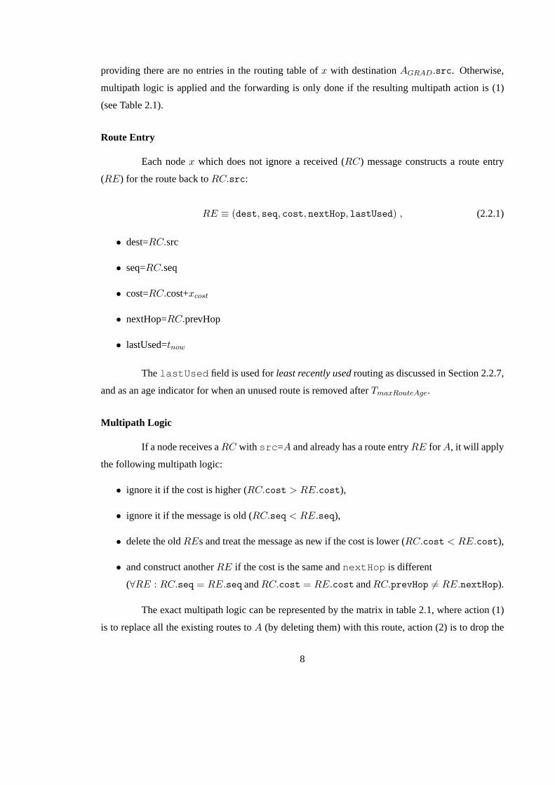
The exact multipath logic can be represented by the matrix in table 2.1, where action (1)

is to replace all the existing routes toA (by deleting them) with this route, action (2) is to drop the

8

Table 2.1: Multipath Logic

Cost/Age RC.seq > RE.seq RC.seq = RE.seq RC.seq < RE.seq

RC.cost < RE.cost purge/add (1) purge/add (1) ignore/drop (2)

RC.cost = RE.cost purge/add (1) add if multipath (3) ignore/drop (2)

RC.cost > RE.cost purge/add (1) ignore/drop (2) ignore/drop (2)

packet and ignore the RC, and action (3) is to add this route to the routing table if it is a multipath

(no otherRE hasRE.nextHop = RC.prevHop andRE.dest = RC.src). If previous routes

were replaced, as in action (1), then forwarding will apply depending on the type. See thegradient

constructionandbacktrace replysections for forwarding of GRAD and RET packets respectively.

Backtrace Reply

After theAGRAD message reaches nodeB, B will send a route controlBRET as a reply

to A, with

RC ≡ (type, seq, retCost, cost, src, dest, prevHop) ,

• type=RET,

• seq=++Bseq,

• retCost=AGRAD.cost,

• cost=0,

• src=B,

• dest=A, and

• prevhop=B.

This message propagates back along the gradient using the return cost (retCost ) to

restrict itself to the shortest return paths, and create routes toB. More precisely, nodes{x|x 6= A}which receiveBRET and for whichBRET.retCost > REA.cost will broadcast aRC with

• retCost=REA.cost

• cost=BRET .cost+xcost,

9

• prevHop=x, and

• other fields have their values set to values in the receivedBRET ,

whereREA is any route entry in the routing table ofx with destinationA. If BRET .retCost ≤REA.cost, BRET is ignored. In place of forwarding, multipath logic is applied if there exist any

route entries ofx with destinationB, and forwarding will only happen if the resulting multipath

action is (1). A route entry with destinationB will be created ifBRET was not ignored by any of

the above.

2.2.6 Passive Route Discovery

Besides network floods, MOR also discovers routes by observing traffic. The data header

(DH) in MOR provides useful routing information:

DH ≡ (type, seq, cost, src, dest, prevHop) .

A data packet from nodeA, forwarded by neighbor nodeB, can be used to construct a route toA if

the route does not already exist. The route entry is constructed similarly as with route control,

• dest=DH.src

• seq=DH.seq

• retCost=DH.cost+xcost

• nextHop=DH.prevHop

• lastUsed=tnow,

wherex is the receiving node.

Return paths to nodes which initiated a network flood could be used if a route is later

required to those nodes, providing the routes have not yet timed out.

While this mechanism is limited to discovering routes taken from data packets passing

through the node, it does not require any significant cost such aspromiscuous mode3. Passive route

discovery discovers routes without the need to broadcast control packets, and is one of the features

of MOR which minimize the use of network floods.3Where packets are not filtered based on their MAC destination address. In non-promiscuous mode, the network

interface card, after examining the packet header, will normally halts the receiver if the packet is not addressed to thehost. Promiscuous mode results in an increase in energy usage, as reception energy as well as energy required to processthe packet by the CPU.

10

2.2.7 Routing and Load Balance

To route a data packetM , a node looks for allREs with dest = M.dest. The data

packet could be forwarded to any of theseREs. For load balancing, differentREs should be

chosen for each consecutive data packet routed to a certain destination. Any number of schemes

may be used: round robin, randomRE, or least recently used. MOR currently uses theleast recently

usedscheme. AssumingREi has the smallestlastUsed value, the data packet is thenunicastto

REi.nextHop andlastUsed is updated to the current time.

When a nodeA initiates a network flood toB, multiple routes are formed, so nodeA will

not need to execute another network flood to findB unless all the paths breaks. Since the nodes

forwarding the network flood now have one or more routes toA, they will not need to execute a

network flood to findA. If A was the base station in a sensor network, none of the nodes sending

data toA will need a network flood. In the best case scenario in which all data gathered are destined

for the base station, a single network flood can set up all necessary routes.

2.2.8 Reliability

Another benefit of having multiple routes at each node is increased hop-by-hop reliabil-

ity. Should a packet fail to transmit with a route entryREi, and another entryREj exists such that

REi.dest = REj .dest, then the packet could be retransmitted usingREj . REi is then put on pro-

bation, and dropped from the table if it causes a number of failures in a row4. In this way, congested

nodes do not immediately break routes, and routes break less often than for other protocols, leading

to longer lasting routes and therefore fewer network floods. Also packet delivery is overall more

reliable, giving higher performance for the protocol.

Retransmission to an alternate route was observed to be helpful when certain nodes drop

packets due to congestion. Other multipath protocols, such as AOMDV [5], use disjoint paths.

Immediate retransmission to congested nodes is a bad idea, since they may still be congested, but

in a disjoint path, intermediate nodes do not have a choice of where to forward a given packet. In

MOR, each node in a path may have a choice of next hops.

2.2.9 Route Maintenance

While routing data packets, each containing a data header (DH), failure to transmit may

eventually remove all routes toDH.dest. MOR will advertise this loss of all routes by use of no

4The current number is 3.

11

route (NR) packets,

NR ≡ (type, seq, src, dest) .

If a nodeA has removed its last route to destinationB due to failure to transmit,A will

broadcast5 a no route packetANR, with

• type=NR,

• seq=Aseq,

• src=A,

• dest=DH.dest.

Each node{x | x 6= B} which receivesANR will search its routing table for aREi with

• dest=ANR.dest, and

• nextHop=ANR.src

If REi does not exist,ANR will be ignored and dropped. Otherwise,REi is removed andx will

search its routing table for aREj with the destinationANR.dest. If REj exists, then the route is

given to nodeA via unicasting a route control (RC) with

RC ≡ (type, seq, retCost, cost, src, dest, prevHop) ,

• type=RT,

• seq=RE.seq,

• retCost=0,

• cost=RE.cost,

• src=RE.dest,

• dest=ANR.src, and

• prevHop=x,

5A local broadcast, as opposed to a network flood.

12

otherwise the nodex has no other route toANR.dest andx will re-broadcastANR with

ANR.nextHop=x.

If node B receivesANR, B will respond with a “I am here” message, which is an RC

with

• type=RT,

• seq=Bseq,

• retCost=0,

• cost=0,

• src=B,

• dest=ANR.src, and

• prevHop=B.

TheRC used in route maintenance is a non-propagating route message (type =RT). Since

no forwarding is done onRT packets, route entry construction is applied if there are no route en-

tries withdest =RC.dest, or multipath logic applies otherwise. See sub-sectionsroute entryand

multipath logicin section 2.2.5.

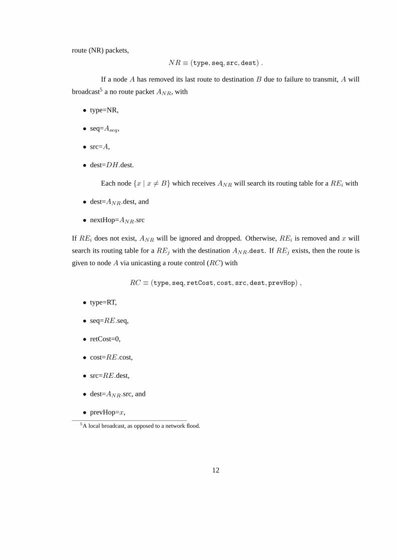
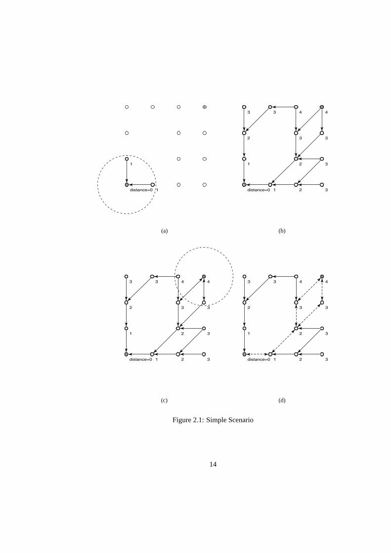
2.3 Simple Scenario

Figure 2.1 shows the behavior of the MOR protocol in a simple scenario. In this topol-

ogy, nodes can reach immediate adjacent and diagonal nodes.Arrows represent table entries or

routes. Distance to nodeA is displayed next to eachnode. Dashedandsolid linesboth represent

communication links.Dashed linesrepresent data traffic.

NodeA has a packet for nodeB, but does not have a route to nodeB. A floods the

network with a packetM indicating a gradient is to be formed, andB is the destination (Fig. 2.1(a)).

A gradient is formed throughout the reachable network withA as the sink (Fig. 2.1(b)).B receives

M and begins the back-trace process by broadcasting a packetR (Fig. 2.1(c)). A receivesR and

data traffic begins (Fig. 2.1(d)).

13

B

A

1distance=0

1

(a)

B

A

1distance=0

1

2

2

2

33

3 3

3

3

4 4

(b)

B

A

1distance=0

1

2

2

2

33

3 3

3

3

4 4

(c)

B

A

1distance=0

1

2

2

2

33

3 3

3

3

4 4

(d)

Figure 2.1: Simple Scenario

14

Chapter 3

Protocol Evaluation

Since simulation was done inns-2[6], protocols readily available inns-2 were considered

for comparison. DSDV and TORA were not considered because only DSR and AODV performed

well in [4] and in our simulations. This section presents a comparison between our protocol, DSR,

and AODV.

3.1 Experimental Setup

Nodes have a range of 250m and were given a large amount of initial energy, measured

in energy units (eu). The default wireless range inns-2is 250m, and correlates to our measurement

of ∼ 300m when PCMCIA 802.11 systems were equipped with 20dB omni-directional antennas.

The receive/transmit energy ratio ofrxtx = 0.5 was taken from that of the Proxim RangeLAN2 card,

Jones et al. [7]. Idle energy was set to a tenth of the reception energy. The link data rate was set to

1 Mbit/sec.

The topologies used in our experiments were randomly generated sensor networks with

an observation area and a base station. Two different setups were considered, a high density net-

work and a low density network. 25 topologies were randomly generated for each density setup as

follows.

3.1.1 High Density

The observation area has a radius of 400m, while the center of the observation area is

1200m from the base station. 100 nodes were randomly placed in the observation area while 24

nodes were randomly placed to relay data to the base station. Since we are interested in getting

15

−200 0 200 400 600 800

−80

0−

600

−40

0−

200

020

0

Distances in meters

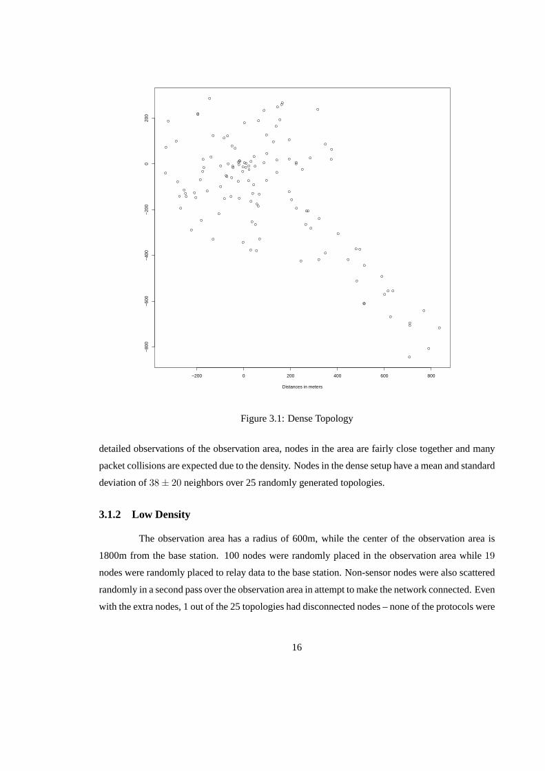
Figure 3.1: Dense Topology

detailed observations of the observation area, nodes in the area are fairly close together and many

packet collisions are expected due to the density. Nodes in the dense setup have a mean and standard

deviation of38± 20 neighbors over 25 randomly generated topologies.

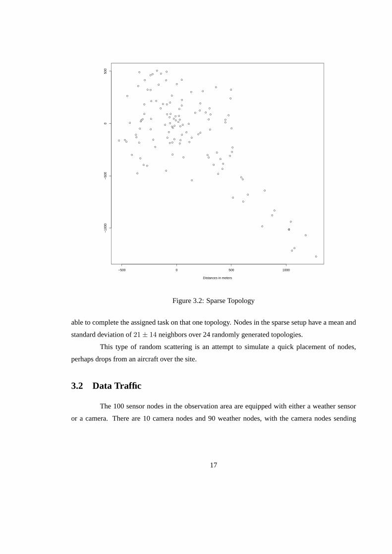
3.1.2 Low Density

The observation area has a radius of 600m, while the center of the observation area is

1800m from the base station. 100 nodes were randomly placed in the observation area while19

nodes were randomly placed to relay data to the base station. Non-sensor nodes were also scattered

randomly in a second pass over the observation area in attempt to make the network connected. Even

with the extra nodes, 1 out of the 25 topologies had disconnected nodes – none of the protocols were

16

−500 0 500 1000

−10

00−

500

050

0

Distances in meters

Figure 3.2: Sparse Topology

able to complete the assigned task on that one topology. Nodes in the sparse setup have a mean and

standard deviation of21± 14 neighbors over 24 randomly generated topologies.

This type of random scattering is an attempt to simulate a quick placement of nodes,

perhaps drops from an aircraft over the site.

3.2 Data Traffic

The 100 sensor nodes in the observation area are equipped with either a weather sensor

or a camera. There are 10 camera nodes and 90 weather nodes, with the camera nodes sending

17

∼ 444KB1 of data and the weather nodes sending7000 bytes of data every hour. Thetaskfor the

entire network amounts to sending∼ 4.94MB of data.

TCP with a large maximum window2 was used to test the protocols under realistic network

conditions. A large packet size of 1400 bytes was selected for TCP since larger packets lead to better

performance in our tests.

3.3 Metrics

In comparing the protocols, the following metrics were used.

• Time: The amount of time it takes for each protocol to complete thetask. In a sensor network,

nodes often take measurements, transmit them to the base station, and then sleep until the

next scheduled sync time. If a protocol is known to complete a task in no more thanX sec,

then the network may safely go to sleepX seconds after a sync. Being able to sleep earlier

saves energy as sleeping devices take considerably less energy than active devices3.

• Energy: The energy use of the entire network. This energy was used for data packet trans-

mission/reception, control packet transmission/reception as well as the node being in the idle

state. In this measurement, we do not include the energy required for computation. Since all

protocols delivered a fixed amount of data, theenergy/dataratio was calculated to express the

energy required for a certain amount of work done.

Furthermore, since the total energy use is dependent on the transmit (tx), receive (rx) and idle

energy use parameters, energy is broken down into tx, rx and idle energies consumed while

completing the task. Energy results for other ratios of tx:rx:idle can be computed from this

breakdown.

• Delivery ratio: Due to collisions, packet drops occur in our experiments, resulting in TCP

retransmissions. The delivery ratio is the TCP measurement of the number of bytes received

over the number of bytes sent.

• Max node energy use: The energy used after completion of thetask by the node with the

highest energy usage in the network. Since this is measured after delivering N bytes, it is an

estimation of the work done before the first node in the network goes down, which can be

1The size of a sample digital camera picture.2A maximum window size of 200 packets was used. TCP never reached this maximum in our experiments.3The WaveLAN I card was measured to have a 177.3mW of power for sleep versus a 1319mW of power for idling [8]

18

computed by N·E/m, where m is the max node energy use and E is the initial energy of all

nodes in the network.

3.4 Results

Results using the above metrics for MOR, DSR and AODV are shown here. The values

presented are the means over the topologies that each protocol was able to complete. Each protocol

is run with 10 different random seeds on each topology.

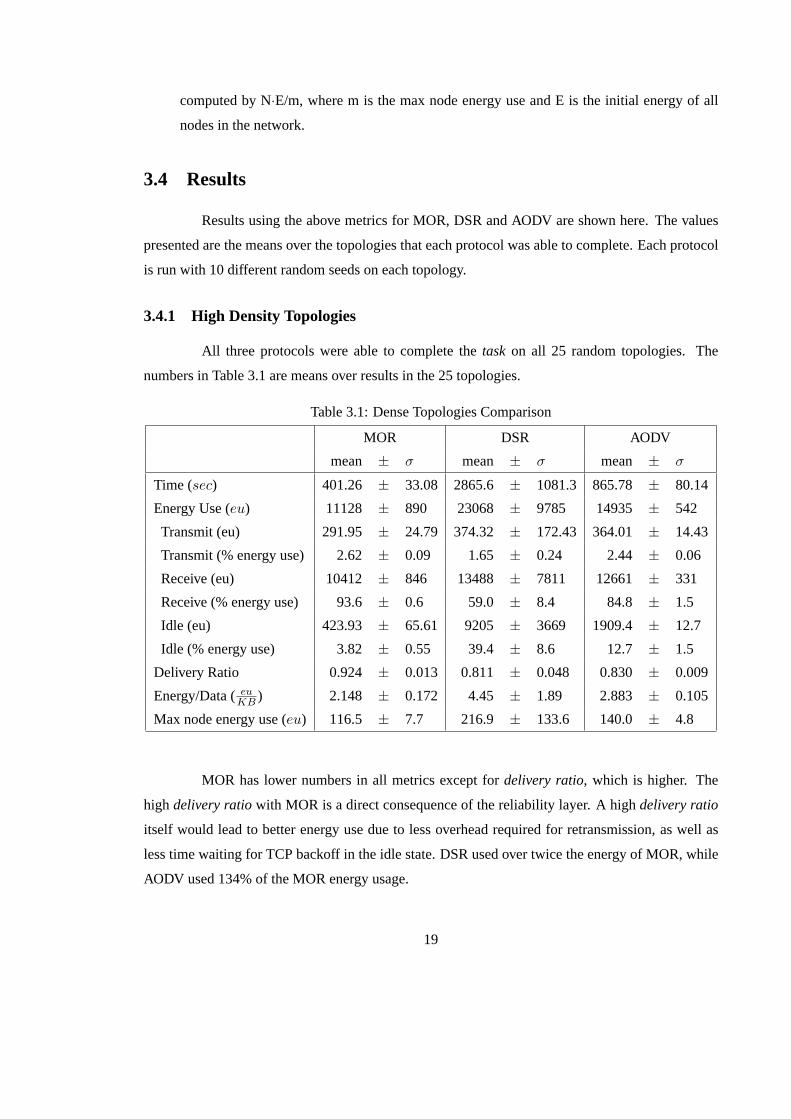
3.4.1 High Density Topologies

All three protocols were able to complete thetask on all 25 random topologies. The

numbers in Table 3.1 are means over results in the 25 topologies.

Table 3.1: Dense Topologies Comparison

MOR DSR AODV

mean ± σ mean ± σ mean ± σ

Time (sec) 401.26 ± 33.08 2865.6 ± 1081.3 865.78 ± 80.14

Energy Use (eu) 11128 ± 890 23068 ± 9785 14935 ± 542

Transmit (eu) 291.95 ± 24.79 374.32 ± 172.43 364.01 ± 14.43

Transmit (% energy use) 2.62 ± 0.09 1.65 ± 0.24 2.44 ± 0.06

Receive (eu) 10412 ± 846 13488 ± 7811 12661 ± 331

Receive (% energy use) 93.6 ± 0.6 59.0 ± 8.4 84.8 ± 1.5

Idle (eu) 423.93 ± 65.61 9205 ± 3669 1909.4 ± 12.7

Idle (% energy use) 3.82 ± 0.55 39.4 ± 8.6 12.7 ± 1.5

Delivery Ratio 0.924 ± 0.013 0.811 ± 0.048 0.830 ± 0.009

Energy/Data (euKB ) 2.148 ± 0.172 4.45 ± 1.89 2.883 ± 0.105

Max node energy use (eu) 116.5 ± 7.7 216.9 ± 133.6 140.0 ± 4.8

MOR has lower numbers in all metrics except fordelivery ratio, which is higher. The

high delivery ratiowith MOR is a direct consequence of the reliability layer. A highdelivery ratio

itself would lead to better energy use due to less overhead required for retransmission, as well as

less time waiting for TCP backoff in the idle state. DSR used over twice the energy of MOR, while

AODV used 134% of the MOR energy usage.

19

The max node energy useindicates that all protocols load balance in about the same

manner (max node energy useis about 1% of the total energy used in all cases), largely because

most of the nodes in the network (100/124 nodes) were sending packets at the same time.

3.4.2 Low Density Topologies

All three protocols were unable to complete thetaskon 1 of the 25 low density topologies

generated. The numbers in Table 3.2 are means over results in 24 topologies.

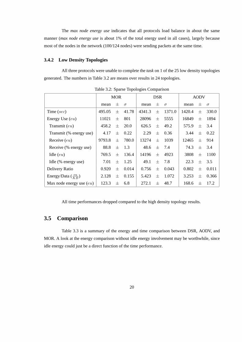
Table 3.2: Sparse Topologies Comparison

MOR DSR AODV

mean ± σ mean ± σ mean ± σ

Time (sec) 495.05 ± 41.78 4341.3 ± 1371.0 1420.4 ± 330.0

Energy Use (eu) 11021 ± 801 28096 ± 5555 16849 ± 1894

Transmit (eu) 458.2 ± 20.0 626.5 ± 49.2 575.9 ± 3.4

Transmit (% energy use) 4.17 ± 0.22 2.29 ± 0.36 3.44 ± 0.22

Receive (eu) 9793.8 ± 780.0 13274 ± 1039 12465 ± 914

Receive (% energy use) 88.8 ± 1.3 48.6 ± 7.4 74.3 ± 3.4

Idle (eu) 769.5 ± 136.4 14196 ± 4923 3808 ± 1100

Idle (% energy use) 7.01 ± 1.25 49.1 ± 7.8 22.3 ± 3.5

Delivery Ratio 0.920 ± 0.014 0.756 ± 0.043 0.802 ± 0.011

Energy/Data (euKB ) 2.128 ± 0.155 5.423 ± 1.072 3.253 ± 0.366

Max node energy use (eu) 123.3 ± 6.8 272.1 ± 48.7 168.6 ± 17.2

All time performances dropped compared to the high density topology results.

3.5 Comparison

Table 3.3 is a summary of the energy and time comparison between DSR, AODV, and

MOR. A look at the energy comparison without idle energy involvement may be worthwhile, since

idle energy could just be a direct function of the time performance.

20

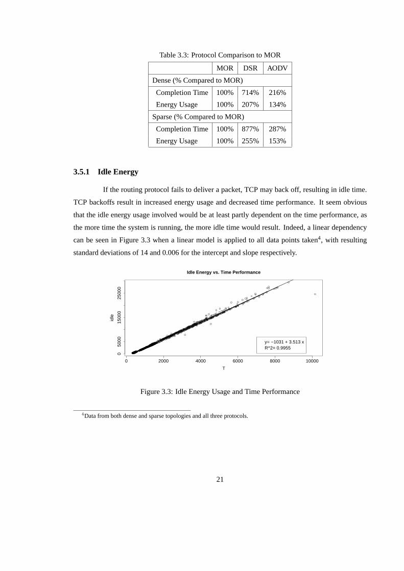
Table 3.3: Protocol Comparison to MOR

MOR DSR AODV

Dense (% Compared to MOR)

Completion Time 100% 714% 216%

Energy Usage 100% 207% 134%

Sparse (% Compared to MOR)

Completion Time 100% 877% 287%

Energy Usage 100% 255% 153%

3.5.1 Idle Energy

If the routing protocol fails to deliver a packet, TCP may back off, resulting in idle time.

TCP backoffs result in increased energy usage and decreased time performance. It seem obvious

that the idle energy usage involved would be at least partly dependent on the time performance, as

the more time the system is running, the more idle time would result. Indeed, a linear dependency

can be seen in Figure 3.3 when a linear model is applied to all data points taken4, with resulting

standard deviations of 14 and 0.006 for the intercept and slope respectively.

0 2000 4000 6000 8000 10000

050

0015

000

2500

0

Idle Energy vs. Time Performance

T

idle

y= −1031 + 3.513 xR^2= 0.9955

Figure 3.3: Idle Energy Usage and Time Performance

4Data from both dense and sparse topologies and all three protocols.

21

Table 3.4: Protocol Comparison to MOR without Idle Energy

MOR DSR AODV

Dense

Receive (rx) + Transmit (tx) Energy10704 13863 13026

rx + tx (% Compared to MOR) 100% 130% 122%

Sparse

Receive (rx) + Transmit (tx) Energy10252 13900 13041

rx + tx (% Compared to MOR) 100% 136% 127%

3.5.2 Energy Without Idle

Table 3.4 show energy comparisons between MOR, AODV, and DSR without idle energy

involvement. With just transmit (tx) and receive (rx) energies considered, all three protocols used

nearly the same amount of energy between sparse and dense topologies. This similarity in energy

use between the dense and sparse topologies is probably just a coincidence, since one should also

note that the transmit energy is higher for the sparse topology while the receive energy is higher for

the dense topology. Since the sparse topologies contain longer routes, more transmissions would be

required to deliver the data, resulting in higher transmission energy usage. Receive energy may be

higher in the dense topology because transmissions reach a larger number of neighbors.

While the increase in idle energy usage was a direct consequence of the amount of time

needed to complete thetask, the receive and transmit energies are due to the actions of the routing

protocol involved. The tx and rx energies are still partly affected by TCP because if TCP retransmit

packets, tx+rx energy would increase. However, retransmissions are due to packet drops, and packet

drop frequency depends on the routing protocol used. Another reliable transport protocol with

backoffs geared toward wireless communication would still need to retransmit lost data. The point

is, tx+rx energy is independent of TCP backoff, and is mostly due to actions taken by the routing

protocol used5.

3.5.3 Performance versus Distance

The drop in time performance in the results from dense to sparse topologies could be

explained by the larger number of hops needed by nodes in the sparse topologies to reach the base

5This assumes everyone is using the same MAC protocol when comparing routing protocols.

22

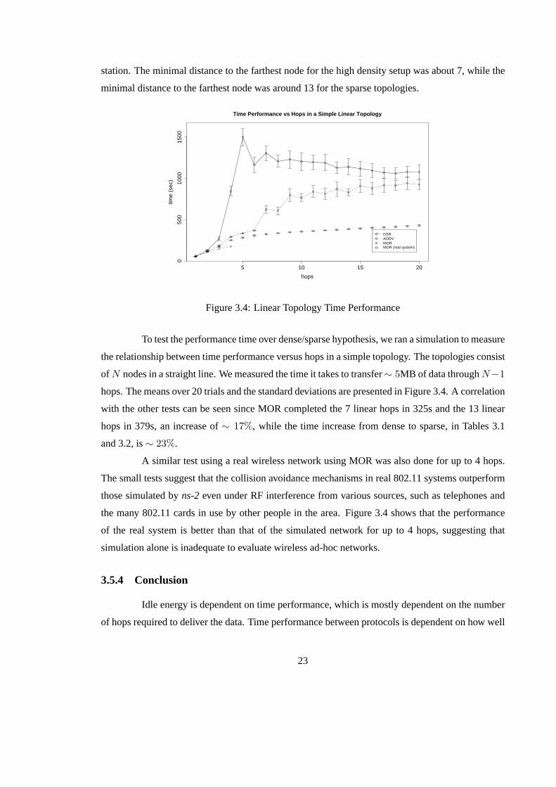
station. The minimal distance to the farthest node for the high density setup was about 7, while the

minimal distance to the farthest node was around 13 for the sparse topologies.

5 10 15 20

050

010

0015

00

Time Performance vs Hops in a Simple Linear Topology

hops

time

(sec

)

oooo

DSRAODVMORMOR (real system)

Figure 3.4: Linear Topology Time Performance

To test the performance time over dense/sparse hypothesis, we ran a simulation to measure

the relationship between time performance versus hops in a simple topology. The topologies consist

of N nodes in a straight line. We measured the time it takes to transfer∼ 5MB of data throughN−1

hops. The means over 20 trials and the standard deviations are presented in Figure 3.4. A correlation

with the other tests can be seen since MOR completed the 7 linear hops in 325s and the 13 linear

hops in 379s, an increase of∼ 17%, while the time increase from dense to sparse, in Tables 3.1

and 3.2, is∼ 23%.

A similar test using a real wireless network using MOR was also done for up to 4 hops.

The small tests suggest that the collision avoidance mechanisms in real 802.11 systems outperform

those simulated byns-2even under RF interference from various sources, such as telephones and

the many 802.11 cards in use by other people in the area. Figure 3.4 shows that the performance

of the real system is better than that of the simulated network for up to 4 hops, suggesting that

simulation alone is inadequate to evaluate wireless ad-hoc networks.

3.5.4 Conclusion

Idle energy is dependent on time performance, which is mostly dependent on the number

of hops required to deliver the data. Time performance between protocols is dependent on how well

23

each protocol handles TCP traffic. Transmit and receive energies are dependent on the actions of

the protocol, independent of TCP backoffs.

MOR handles TCP data better than AODV and DSR, as seen from the time performance

in Tables 3.1 and 3.2. From the transmit and receive energies shown in Table 3.4, MOR still has

superior energy performance even if the time to completion is not taken into account. It can be

concluded that MOR is more energy and time efficient than the other protocols measured, in part

because of its multipath nature and in part because more of its packets reached their final destination.

24

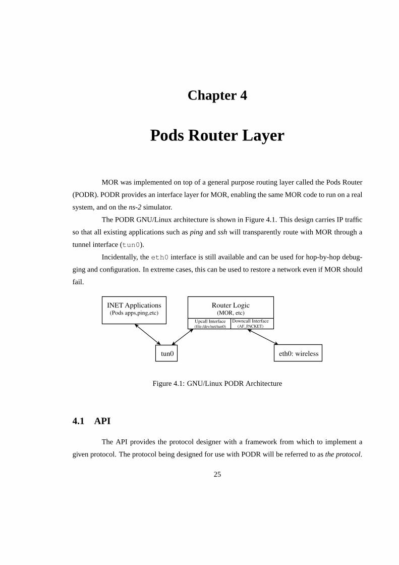
Chapter 4

Pods Router Layer

MOR was implemented on top of a general purpose routing layer called the Pods Router

(PODR). PODR provides an interface layer for MOR, enabling the same MOR code to run on a real

system, and on thens-2simulator.

The PODR GNU/Linux architecture is shown in Figure 4.1. This design carries IP traffic

so that all existing applications such asping andsshwill transparently route with MOR through a

tunnel interface (tun0 ).

Incidentally, theeth0 interface is still available and can be used for hop-by-hop debug-

ging and configuration. In extreme cases, this can be used to restore a network even if MOR should

fail.

tun0

Router Logic (MOR, etc)

Upcall Interface (file:/dev/net/tun0)

Downcall Interface (AF_PACKET)

INET Applications (Pods apps,ping,etc)

eth0: wireless

Figure 4.1: GNU/Linux PODR Architecture

4.1 API

The API provides the protocol designer with a framework from which to implement a

given protocol. The protocol being designed for use with PODR will be referred to asthe protocol.

25

The following is an overall description of the PODR API. The exact API is not finalized at this time.

The primary elements in PODR are callbacks, queues, and interfaces.

4.1.1 Callbacks

The protocol must provide PODR with a set of callback functions in order to trap events:

• init - Called during PODR initialization so the protocol may perform initialization,

• recv - Called whenever a packet arrives from the default interface,

• queue - Called when a queue item times out,

• sendFail - Called when packet transmission fails,

• onStart - Called when all interfaces are up, as opposed to init where interfaces are not yet

initialized,

• printRouteTable - Called for debugging purposes in order to examine the routing tables.

The protocol fills a structure (struct router ) with these callbacks and makes them

known to PODR via thePODR_REGISTER()macro.

4.1.2 Queues

Since PODR handles execution scheduling, a time priority queue (podrQueue ) is pro-

vided as a means for the protocol to execute timed events. One or morepodrQueue may be created

by the protocol in order to execute timed events. Queues are given to PODR by use of

podr_insertQueue(podrQueue *)

Timed out events (queue entries) are passed back to the protocol via the queue callback as mentioned

above.

4.1.3 Interfaces

Interfaces are abstracted by use ofstruct interface_t . This structure contains

receive and send functions, filled in by a constructor function provided by the interface imple-

mentation. Interfaces may be constructed by the protocol during initialization by calling the pro-

vided constructor, giving the interface a receive callback, then handing the interface to PODR via

iftable_insert(struct interface_t *) .

26

Currently, the Ethernet and tunnel interfaces are implemented in PODR. In our setup,

Ethernet is the default interface created by PODR, while the tunnel interface was created by MOR

as a means to communicating with applications.

4.1.4 Node Multiplexing

Our implementation avoids allocating memory dynamically due to the need for precise

control of memory. Memory is laid out before deployment and the maximum amount of memory

used by the protocol is known. This accommodates the limited memory available to many small

systems considered for network sensors.

While the protocol implementation was made efficient for one node,ns-2needs to mul-

tiplex the node state in order to simulate multiple nodes. In order for thens-2 implementation to

correctly multiplex the node state, the protocol must register such state information by use of the

PODR_REGISTER_STATE()macro. This macro does nothing in the real system implementation.

The simulation implementation of PODR makes a copy of the state information for each

node simulated and does a context switch while processing each node. For the protocol to work

correctly using the simulation implementation, the protocol must make sure state information is

registered correctly. This scheme may seem complicated, but we consider the real system imple-

mentation a higher priority than the simulation.

27

Chapter 5

Related Work

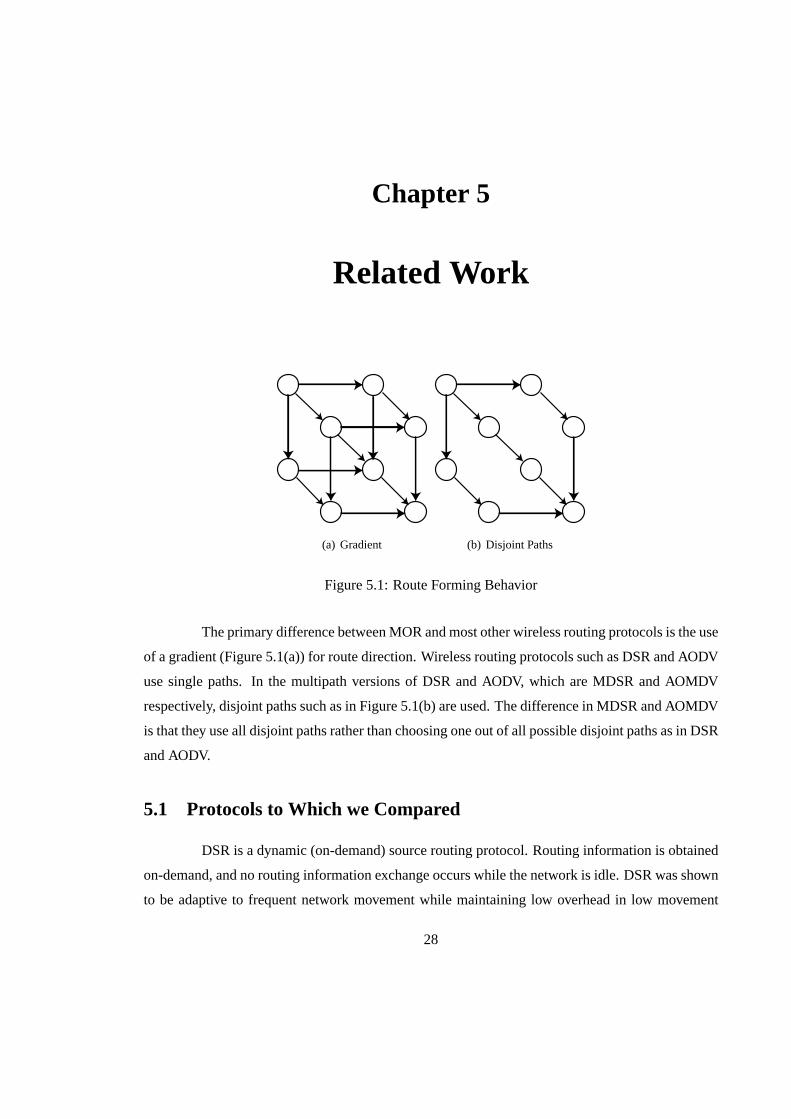
(a) Gradient (b) Disjoint Paths

Figure 5.1: Route Forming Behavior

The primary difference between MOR and most other wireless routing protocols is the use

of a gradient (Figure 5.1(a)) for route direction. Wireless routing protocols such as DSR and AODV

use single paths. In the multipath versions of DSR and AODV, which are MDSR and AOMDV

respectively, disjoint paths such as in Figure 5.1(b) are used. The difference in MDSR and AOMDV

is that they use all disjoint paths rather than choosing one out of all possible disjoint paths as in DSR

and AODV.

5.1 Protocols to Which we Compared

DSR is a dynamic (on-demand) source routing protocol. Routing information is obtained

on-demand, and no routing information exchange occurs while the network is idle. DSR was shown

to be adaptive to frequent network movement while maintaining low overhead in low movement

28

rates [9]. DSR was also shown to be favorable in a performance comparison [4] with TORA,

DSDV, and AODV. The problem in DSR lies in its limited scalability, as source routing packets get

larger with increasing hops, and in the use of promiscuous mode for route caching and response, as

promiscuous mode is very demanding in terms of energy usage.

AODV is also an on-demand routing protocol. It performs nearly as well as DSR [4], but

without the scaling problem and promiscuous mode usage of DSR. The problem of AODV lies in its

need to initiate route discovery very often, which decreases delivery ratio, increases energy usage,

and decreases time performance.

5.2 Gradient Routing Protocols

Under ideal conditions, a gradient contains the shortest paths back to the source of the

request and is used in forwarding packets to nodes that are closer to a given destination. In contrast,

distance vector finds a single shortest path to the destination. A gradient may not always find the

optimal path. Due to collisions, nodes on the optimal path may not be able to forward their packets

in N transmissions, whereN is the maximum number of retransmissions allowed. Consequently, a

non-optimal path may be used by any of the gradient forming protocols.

In MOR, the gradient process and the back-trace process may each create routes with

different costs. Assume the gradient process forms routes of costN and the back-trace process

forms routes of costM . Because data packets also construct and update routes in MOR, the routes

will eventually converge to have costmin(N,M). The result is MOR has a higher probability of

finding better routes and of finding the optimal route.

GRAd [10] is another on-demand routing protocol making use of gradient routing, but

has not yet been compared in any studies. Gradient Routing Protocol (GRAd) was developed at the

MIT Media Laboratory. GRAd is patented and currently used in TephraNet. TephraNet was placed

in a sensor network for testing in collaboration with the Pods project. TephraNet computers and

radios were placed in Pods enclosures, summer 2001. GRAd was not tested in this work since a

GRAd simulation forns-2is not available to us.

While GRAd and MOR both use gradients for route direction, GRAd emphasizes low

end-to-end latencies by forgoing the use of unicast in favor of broadcast. Given multiple shortest

path routes to a destination, the result is every node in all the shortest paths will forward data

packets. Given many shortest paths, this would lead to a high level of redundant transmission and

consequently inefficient energy use.

29

Directed Diffusion [3] is a different communications paradigm for network sensors. Dif-

fusion is mentioned here due to its use of the gradient behavior to propagate interest. Although

Diffusion is designed for data delivery, Diffusion is not strictly a routing protocol. Instead of nodes

collecting data and sending them to the base on a fixed schedule, the base propagates an “interest”,

which form a gradient and node(s) with the interest “reinforce” the gradient paths in order to deliver

data. Meaningful comparison with MOR would be difficult given such different scenarios.

5.3 Protocols with Poor Performance

The Temporally Ordered Routing Algorithm (TORA) and Destination-Sequenced Distance-

Vector (DSDV) Routing were also shown in [4], but were not discussed in our paper because both

those protocols failed to perform thetask in most of the topologies considered. The failure could

be because the simulations given in [4] were only 1 to 5 hops, while some nodes in our topologies

have a minimal distance of 12 hops to the base station. Aside from the longer hops, previous studies

only used constant bit rate (CBR). Unlike TCP, CBR traffic is usually unidirectional.

5.4 Multipath

Multipath routing is gaining in popularity, as there are works extending both DSR and

AODV to use multipaths. Nasipuri et al. [11] studied two theoretical multipath variations of DSR

(MDSR). Since MOR uses a gradient, MOR supports as many alternate routes as the network will

provide, but MDSR only extends up to one additional route per destination neighbor node. The mul-

tipath version of AODV, the Ad-hoc On-demand Multipath Distance Vector (AOMDV) Protocol [5],

is able to handle different number of hop counts1 and link-disjoint paths. One major difference is

that MOR does not have the restriction that paths to a destination be disjoint. While the result

may be less even load balancing, we claim it also results in more choices at each node and more

reliability, and therefore more efficient data transmissions.

5.5 DLAR

The Dynamic Load-Aware Routing (DLAR) protocol, Sung [12], uses load as a primary

metric. DLAR is a single path protocol, first constructing disjoint paths and then selecting the one

1AOMDV uses shortest paths, but is able to accept longer paths by having the destination be less strict about acceptingroutes which are longer in distance.

30

path with the lowest load2. Load information is also piggybacked on data packets so as to monitor

congestion, and constructing new paths in order to avoid congestion. When congestion is detected,

DLAR nodes flood the network to construct a new route. This frequent flooding is in contrast to

the MOR behavior of minimizing the number of floods, while MOR also deals with congestion by

using all available multipaths.

2The lowest load is computed based on the number of packets in interface queues of the nodes in the path.

31

Chapter 6

Future Work

MOR was designed with a real system in mind. The MOR routing code used in this paper

was designed to work under the GNU/Linux operating system. MOR is able to run onns-2due to

an ns-2wrapper layer which emulates sockets. This was done to reduce the cost of debugging in

a real system. The result is a much more robust implementation than the initialns-2only version.

The logical next step, which is in progress, is to deploy nodes at a test site and gather performance

data for MOR in a real system.

Another metric to consider iswork to network partition, where work is the amount of data

delivered. This is similar totime to network partitiondescribed by Jones et al. [7], which is the time

until a number of critical nodes go down and the network partitions as a result. Since MOR does

work faster than DSR and AODV, MOR may have a smaller time to network partition but would

have gotten more work done at the time of partition. Work to network partition is a better metric in

that it does not penalize protocols which deliver data faster.

32

Chapter 7

Conclusion

Reasonable sensor network topologies were simulated. Distances to the base station and

the size of the observation area were taken from an actual observation site where we have done pre-

liminary deployments. Nodes were randomly scattered to discourage bias in choosing the topologies

used in evaluating performance. MOR was able to perform better in terms of time and energy use

for a particular task under both dense and sparse network settings. MOR used noticeably less energy

in the simulations presented, and completed thetasksignificantly faster in some cases.

For the dense topology setup where there is a high rate of collisions, DSR used twice the

energy MOR used and AODV used 134%, while MOR completed thetaskmore than seven times

as fast as DSR and over twice as fast as AODV. In low density topologies, where nodes have fewer

neighbors and consequently experience fewer collisions, DSR and AODV used 255% and 153% the

energy MOR used respectively. The time performance of DSR and AODV as compared to MOR

was even worst for the sparse topologies, as the hop count increased.

MOR was able to achieve its comparatively efficient energy use by fully leveraging mul-

tipaths. Although MOR and AODV find nodes on the network in nearly the same way (through

flooding and route entries at each node), MOR’s attempt to minimizes the number of network floods

through the use of multipaths yielded a much better energy performance than AODV.

MOR has been used since August 2002 to route packets in PODS networks. This experi-

ence led to some of the current refinements of MOR.

33

Appendix A

MOR Specification

The following is the specification followed by the current implementation of MOR. A

implementation compatible with our own can be built from this specification together with details

given in Chapter 2. This specification is subject to change.

A.1 Constants

The current version is 1.

The reliability threshold is 3. This is the number of times a link must fail to transmit a

packet before it is removed.

TmaxRouteAge is 1000 sec. Route entries are removed if unused forTmaxRouteAge amount

of time.

A.2 Packets and Packet Headers

Packet structures are formatted to display with 4 byte per rows.

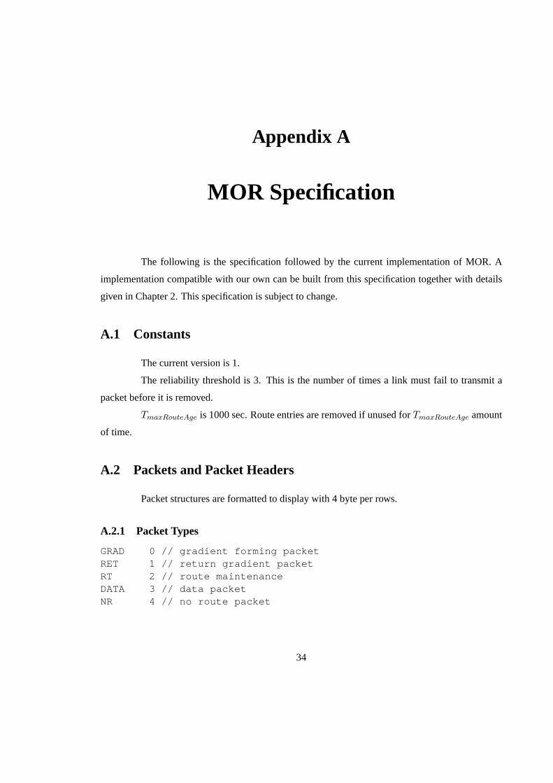
A.2.1 Packet Types

GRAD 0 // gradient forming packetRET 1 // return gradient packetRT 2 // route maintenanceDATA 3 // data packetNR 4 // no route packet

34

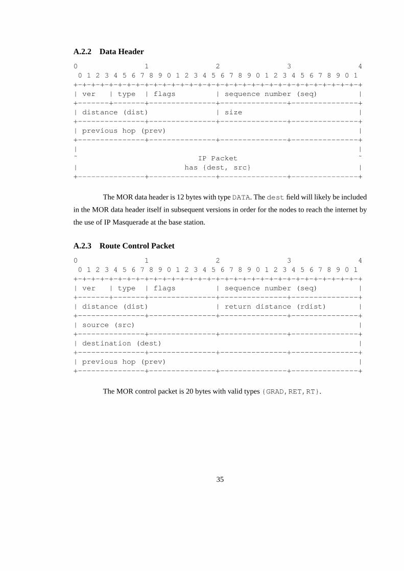
A.2.2 Data Header

0 1 2 3 40 1 2 3 4 5 6 7 8 9 0 1 2 3 4 5 6 7 8 9 0 1 2 3 4 5 6 7 8 9 0 1

+-+-+-+-+-+-+-+-+-+-+-+-+-+-+-+-+-+-+-+-+-+-+-+-+-+-+-+-+-+-+-+-+| ver | type | flags | sequence number (seq) |+-------+-------+---------------+---------------+---------------+| distance (dist) | size |+---------------+---------------+---------------+---------------+| previous hop (prev) |+---------------+---------------+---------------+---------------+| |˜ IP Packet ˜| has {dest, src} |+---------------+---------------+---------------+---------------+

The MOR data header is 12 bytes with typeDATA. Thedest field will likely be included

in the MOR data header itself in subsequent versions in order for the nodes to reach the internet by

the use of IP Masquerade at the base station.

A.2.3 Route Control Packet

0 1 2 3 40 1 2 3 4 5 6 7 8 9 0 1 2 3 4 5 6 7 8 9 0 1 2 3 4 5 6 7 8 9 0 1

+-+-+-+-+-+-+-+-+-+-+-+-+-+-+-+-+-+-+-+-+-+-+-+-+-+-+-+-+-+-+-+-+| ver | type | flags | sequence number (seq) |+-------+-------+---------------+---------------+---------------+| distance (dist) | return distance (rdist) |+---------------+---------------+---------------+---------------+| source (src) |+---------------+---------------+---------------+---------------+| destination (dest) |+---------------+---------------+---------------+---------------+| previous hop (prev) |+---------------+---------------+---------------+---------------+

The MOR control packet is 20 bytes with valid types{GRAD,RET,RT} .

35

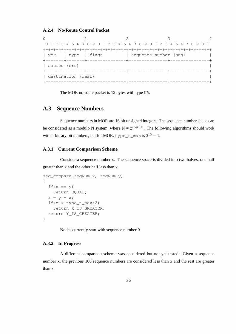
A.2.4 No-Route Control Packet

0 1 2 3 40 1 2 3 4 5 6 7 8 9 0 1 2 3 4 5 6 7 8 9 0 1 2 3 4 5 6 7 8 9 0 1

+-+-+-+-+-+-+-+-+-+-+-+-+-+-+-+-+-+-+-+-+-+-+-+-+-+-+-+-+-+-+-+-+| ver | type | flags | sequence number (seq) |+-------+-------+---------------+---------------+---------------+| source (src) |+---------------+---------------+---------------+---------------+| destination (dest) |+---------------+---------------+---------------+---------------+

The MOR no-route packet is 12 bytes with typeNR.

A.3 Sequence Numbers

Sequence numbers in MOR are 16 bit unsigned integers. The sequence number space can

be considered as a modulo N system, where N =2seqBits. The following algorithms should work

with arbitrary bit numbers, but for MOR,type_t_max is 216 − 1.

A.3.1 Current Comparison Scheme

Consider a sequence number x. The sequence space is divided into two halves, one half

greater than x and the other half less than x.

seq_compare(seqNum x, seqNum y){

if(x == y)return EQUAL;

z = y - x;if(z > type_t_max/2)

return X_IS_GREATER;return Y_IS_GREATER;

}

Nodes currently start with sequence number 0.

A.3.2 In Progress

A different comparison scheme was considered but not yet tested. Given a sequence

number x, the previous 100 sequence numbers are considered less than x and the rest are greater

than x.

36

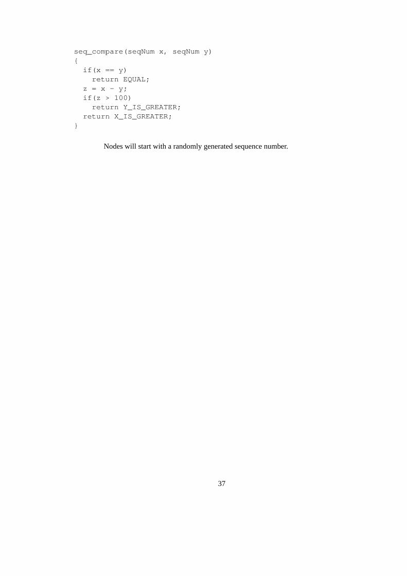
seq_compare(seqNum x, seqNum y){

if(x == y)return EQUAL;

z = x - y;if(z > 100)

return Y_IS_GREATER;return X_IS_GREATER;

}

Nodes will start with a randomly generated sequence number.

37

Bibliography

[1] Darpa.<http://dtsn.darpa.mil/ixo/sensit.asp> , 2001.

[2] Edoardo Biagioni and Kent Bridges. The application of remote sensor technol-

ogy to assist the recovery of rare and endangered species.International Jour-

nal of High Performance Computing Applications, 16(3), 2002. Available from

http://www.ics.hawaii.edu/˜ esb/prof/pub/ijhpca02.html.

[3] Chalermek Intanagonwiwat, Ramesh Govindan, and Deborah Estrin. Directed diffusion: a

scalable and robust communication paradigm for sensor networks. InMobile Computing and

Networking, pages 56–67, 2000.

[4] Josh Broch, David A. Maltz, David B. Johnson, Yih-Chun Hu, and Jorjeta Jetcheva. A per-

formance comparison of multi-hop wireless ad hoc network routing protocols. InMobile

Computing and Networking, pages 85–97, 1998.

[5] Asis Nasipuri and Samir R. Das. On-Demand multipath routing for mobile ad hoc networks.

In 8th Annual IEEE Internation Conference on Computer Communications and Networks (IC-

CCN), Boston MA, pages 64–70, 1999.

[6] Kevin Fall and Kannan Varadhan.The ns Manual. The VINT Project, UC Berkeley, LBL,

USC/ISI, and Xerox PARC, 2002.

[7] Christine E. Jones, Krishna M. Sivalingam, Prathima Agrawal, and Jyh-Cheng Chen. A survey

of energy efficient network protocols for wireless networks.Wireless Networks, 7(4):343–358,

2001.

[8] Laura Marie Feeney. An energy consumption model for performance analysis of routing pro-

tocols for mobile ad hoc networks. InProceedings of the 45th IETF Meeting, MANET Work-

ing Group, 1999. Available from http://www.ietf.org/proceedings/99jul/ slides/manet-feeney-

99jul.pdf.

38

[9] David B Johnson and David A Maltz. Dynamic source routing in ad hoc wireless networks. In

Imielinski and Korth, editors,Mobile Computing, volume 353. Kluwer Academic Publishers,

1996.

[10] Robert Poor. Self-organizing network. Patent 6,028,857, United States,

2000. Gradient Routing is also described in a paper available at

http://www.media.mit.edu/pia/Research/ESP/texts/poorieeepaper.pdf.

[11] Asis Nasipuri, Robert Castaneda, and Samir R. Das. Peformance of multipath routing for on-

demand protocols in mobile ad hoc networks.ACM/Baltzer Mobile Networks and Applications

(MONET), 6:339–349, 2001.

[12] Sung-Ju Lee.Routing and Multicasting Strategies in Wireless Mobile Ad hoc Networks. PhD

thesis, University of California Los Angeles, 2000.

39