Embed Size (px)
Citation preview

NOTE TO USERS
Page(s) missing in number only; text follows. The manuscript was microfilmed as received.
121-122
This reproduction is the best copy available.
UMI®

MULTIDIMENSIONAL GOALS OF FARMERS IN THE BEEF CATTLE AND DAIRY INDUSTRIES
A Dissertation
Submitted to the Graduate Faculty of the Louisiana State University and
Agricultural and Mechanical College In partial fulfillment of the
requirements for the degree of Doctor of Philosophy
in
The Department of Agricultural Economics and Agribusiness
By Aydin Basarir
B.S., Ankara University, 1991 M.S., University of Delaware, 1997
August, 2002

UMI Number: 3063042
________________________________________________________
UMI Microform 3063042
Copyright 2002 by ProQuest Information and Learning Company.
All rights reserved. This microform edition is protected against
unauthorized copying under Title 17, United States Code.
____________________________________________________________
ProQuest Information and Learning Company 300 North Zeeb Road
PO Box 1346 Ann Arbor, MI 48106-1346

ii
DEDICATION
This work is dedicated to my wife, Bahtinur Basarir, and our two children, Nur Sena and
Kerem Edip.
iii
ACKNOWLEDGEMENTS
There are a number of people who have contributed to this dissertation and made my
study in the U.S. an exciting and rewarding experience. First, I would like to thank Dr. Jeffrey
M. Gillespie, my major professor, for his guidance, support, and understanding since the
beginning of the Ph.D. program at Louisiana State University. His guidance, and prompt
response to any request were invaluable. His valuable discussion and involvement in this
research have served to improve the focus, organization and result of the dissertation.
I would like to thank to Dr. Richard F. Kazmierczak, Dr. Lonnie R. Vandeveer, Dr.
Hector O. Zapata, and Dr. M. Dek Terrell for their encouragement, support, cooperation,
suggestions and careful review of this dissertation.
My sincere thanks go to both the former and new Heads of the Department of
Agricultural Economics and Agribusiness, Dr. Kenneth Paxton, Dr. Albert Ortego and Dr. Gail
L. Cramer, and the faculty, staff, and my fellow graduate student friends for their help,
encouragement, support and friendship during my stay at LSU.
Special thanks goes to Gazi Osman Pasa University, and the Turkish Higher Education
Council for giving me the opportunity and financial support to enhance my professional
capabilities.
Finally, sincere thanks are extended to my wife, Bahtinur, beloved children, Nur Sena
and Kerem Edip, and my whole family and friends for their love, prayer, and encouragement.

iv
TABLE OF CONTENTS
DEDICATION .............................................................................................................................. ii ACKNOWLEDGEMENTS..........................................................................................................iii LIST OF TABLES ......................................................................................................................vii LIST OF FIGURES...................................................................................................................... ix ABSTRACT .............................................................................................................................. x CHAPTER 1. INTRODUCTION ................................................................................................ 1 1.1. U.S. and Louisiana Beef Cattle and Dairy Industries............................................................. 3 1.2. Problem Statement ................................................................................................................ 5 1.3. Justification ........................................................................................................................... 9 1.4. Objectives............................................................................................................................ 11 1.4.1. General Objectives............................................................................................................. 11 1.4.2. Specific Objectives ............................................................................................................ 11 1.5. The General Procedures and Outline of the Dissertation ..................................................... 11 CHAPTER 2. LITERATURE REVIEW.................................................................................... 13 2.1. Methods that Have Been Used by Previous Researchers to Elicit Goal Hierarchies............ 13 2.2. The Basic Pair-Wise Comparison........................................................................................ 13 2.2.1. Fuzzy Pair-Wise Comparison Method ............................................................................... 15 2.2.2. Magnitude Estimation........................................................................................................ 16 2.2.3. Analytic Hierarchy Process................................................................................................ 17 2.3. Goal Hierarchy Studies........................................................................................................ 17 CHAPTER 3. METHODOLOGY AND DATA COLLECTION............................................... 26 3.1. Utility Maximization ........................................................................................................... 27 3.2. Fuzzy Pair-Wise Comparison.............................................................................................. 27 3.3. Simple Ranking of Goals..................................................................................................... 30 3.4. Nonparametric Statistical Analysis...................................................................................... 31 3.4.1. Friedman’s Test................................................................................................................ 31 3.4.2. Kendall’s W ..................................................................................................................... 33 3.4.3. Distance Function ............................................................................................................ 33 3.5. Testing for Consistency Between the Fuzzy Pair-Wise Comparison Method and the
Simple Ranking of Goals..................................................................................................... 34 3.6. Logistic Model .................................................................................................................... 35 3.7. Seemingly Unrelated Regression Model (SUR) .................................................................. 38 3.8. The Explanatory Variables that Affect the Weight of the Goals.......................................... 41 3.8.1. Section I: Production Characteristics ................................................................................. 42 3.8.2. Section II: Risk, Social Capital, and Environmental Attitudes.......................................... 47 3.8.2.1. Risk Attitude................................................................................................................. 47 3.8.2.2. Social Capital................................................................................................................ 48

v
3.8.2.3. The Environmental Attitude.......................................................................................... 50 3.8.3. Section III: Producer and Farm Characteristics.................................................................. 51 3.9. Test Statistics ...................................................................................................................... 55 3.9.1. Multicollinearity Analysis ................................................................................................. 55 3.9.2. Testing for Heteroscedasticity ........................................................................................... 57 3.10. The Selection and Discussion of Explanatory Variables for Each Equation........................ 59 3.11. Data Collection.................................................................................................................... 61 3.11.1. Survey Sample ................................................................................................................. 61 3.11.2 Survey Administration ..................................................................................................... 62 CHAPTER 4. RESULTS AND DISCUSSION ......................................................................... 63 4.1. Return Rate and the Statistics of the Survey for Beef Cattle Producers............................... 63 4.2. Return Rate and the Statistics of the Survey for Dairy Producers........................................ 67 4.3. The Fuzzy Pair-Wise and Simple Ranking Goal Weights for the Beef Cattle Producers..... 70 4.4. The Fuzzy Pair Wise and Simple Ranking Goal Weights for the Dairy Producers.............. 78 4.5. Fuzzy Pair-Wise Goal Weights by Categories for Beef Cattle Producers............................ 81 4.6. Fuzzy Pair-Wise Goal Weight by Categories for Dairy Producers ...................................... 84 4.7. Testing for Consistency Between the Fuzzy Pair-Wise Comparison and the Simple
Ranking Methods for Beef Cattle Producers ....................................................................... 84 4.8. Testing for Consistency Between the Fuzzy Pair-Wise Comparison and Simple Ranking
Methods for Dairy Producers............................................................................................... 87 4.9. Determining the Effect of Exogenous Variables on Goal Hierarchy ................................... 88 4.9.1. Results of the Multicollinearity Test for Beef Cattle Producers ......................................... 88 4.9.2. Results of the Multicollinearity Tests for Dairy................................................................. 94 4.9.3. Variable Selection Through the Stepwise Regression Procedure....................................... 94 4.9.4. Results of the Heteroscedasticity Tests ............................................................................ 101 4.9.5. Results of the Contemporaneous Correlation Test ........................................................... 103 4.10. The Results of Seemingly Unrelated Logistic Regression (SULR) Models ...................... 104 4.10.1. Results of the Seemingly Unrelated Logistic Regression Analysis for Beef Cattle
Producers ....................................................................................................................... 104 4.10.2. Results of the Seemingly Unrelated Logistic Regression Analysis for Dairy Producers 112 4.10.3. Results of the Combined Seemingly Unrelated Logistic Regression Analysis for Beef
Cattle and Dairy Producers............................................................................................. 118 CHAPTER 5. SUMMARY AND CONCLUSIONS................................................................ 125 5.1. Summary and Conclusions ................................................................................................. 125 5.2. Limitations of the Dissertation............................................................................................ 133 5.3. Needs for Further Research ................................................................................................ 134 REFERENCES.......................................................................................................................... 135 APPENDIX 1. THE SURVEY QUESTIONNAIRE FOR BEEF CATTLE PRODUCERS...... 142 APPENDIX 2. THE SURVEY QUESTIONNAIRE FOR DAIRY PRODUCERS ................... 151

vi
APPENDIX 3. LETTER INCLUDED IN THE FIRST MAIL OUT FOR BEEF CATTLE PRODUCERS................................................................................................... 163
APPENDIX 4. LETTER INCLUDED IN THE FIRST MAIL OUT FOR DAIRY PRODUCERS................................................................................................... 164 APPENDIX 5. POSTCARD FOR BEEF CATTLE PRODUCERS .......................................... 165 APPENDIX 6. POSTCARD FOR DAIRY PRODUCERS ....................................................... 166 APPENDIX 7. LETTER IINCLUDED IN THE SECOND MAIL OUT FOR BEEF CATTLE
PRODUCERS................................................................................................... 167 APPENDIX 8. LETTER INCLUDED IN THE SECOND MAIL OUT FOR DAIRY
PRODUCERS................................................................................................... 168 VITA .......................................................................................................................... 169

vii
LIST OF TABLES Table 1.1. Summary of Estimated Net Returns per Cow for Beef Cow-Calf Production in
Louisiana……………………………………………………………………………....7 Table 1.2. Summary of Estimated Net Returns per Cow for Dairy Production in Louisiana…….7 Table 4.1. Data Definitions and Descriptive Statistics For Beef Cattle Producers. ..................... 64 Table 4.2. Data Definitions and Descriptive Statistics For Dairy Producers. .............................. 68 Table 4.3. Descriptive Statistics of Goal Scores for Beef Cattle Producers Who Had 1-19
Animals. ..................................................................................................................... 73 Table 4.4. Descriptive Statistics of Goal Scores for Beef Cattle Producers Who Had 20-49
Animals. ..................................................................................................................... 73 Table 4.5. Descriptive Statistics of Goal Scores for Beef Cattle Producers Who Had 50-99
Animals. ..................................................................................................................... 76 Table 4.6. Descriptive Statistics of Goal Scores for Beef Cattle Producers Who Had 100+
Animals. ..................................................................................................................... 76 Table 4.7. Goal Weight of All Categories Ranked by Overall Mean for Beef Cattle Producers. 77 Table 4.8. Descriptive Statistics of Goal Scores for Dairy Producers. ........................................ 80 Table 4.9. Categorical Goal Weights of Beef Cattle Producers. ................................................. 82 Table 4.10. Categorical Goal Scores of Dairy Producers. ........................................................... 85 Table 4.11. Spearman Rank Correlation Test Statistics for Consistency of the Goal Scores in the Fuzzy Pair-Wise and Simple Ranking Procedures for Beef Cattle Producers. 88 Table 4.12. Spearman Rank Correlation Test Statistics for Consistency of the Goal Scores in the Fuzzy Pair-Wise and Simple Ranking Procedures for Dairy Producers. ......... 88 Table 4.13. Pearson Correlation Coefficients of Independent Variables for Beef Cattle Producers.................................................................................................................. 90 Table 4.14. The Results of the Multicollinearity VIF and CI Tests for Beef Cattle Producers.... 93 Table 4.15. Pearson Correlation Coefficients of Independent Variables for Dairy Production. .. 95 Table 4.16. The Results of the Multicollinearity VIF and CI Tests for Dairy Producers. ........... 98

viii
Table 4.17 . Heteroscedasticity Test Results for Beef Cattle and Dairy Variables.................... 102 Table 4.18. The Regression of Goal Scores for Beef Cattle Producers. .................................... 105 Table 4.19. The Regression of Goal Scores for Dairy Producers. ............................................. 114 Table 4.20. The Regression of Goal Scores for Beef Cattle and Dairy Producers..................... 120
ix
LIST OF FIGURES Figure 2.1. Analytic Hierarchy Process for Making Comparison Between Gi and Gj. ................ 17 Figure 3.1. Fuzzy Pair-Wise Approach for Making Comparison Between X and Y................... 29 Figure 3.2 The Logistic Transformation. .................................................................................... 36

x
ABSTRACT
Farm firm decision making processes have long been of concern to agricultural
economists. The concept of maximizing utility rather than profit is an important concept in
multidimensional goal research. The prevalence of low or negative net returns in Louisiana beef
and dairy production leads to the hypothesis that goals other than profit maximization compete
strongly in producers’ decisions. The objective of this study is to determine the hierarchy of
goals that motivate beef and dairy producers and evaluate them in a multi-dimensional
framework.
Seven goals were evaluated in producer decision making: Maintain and Conserve Land,
Maximize Profit, Increase Farm Size, Avoid Years of Loss / Low Profit, Increase Net Worth,
Have Time for Other Activities, and Have Family Involved in Agriculture. Each goal’s weight is
its importance in the measurement of the farmer’s utility. Weights were elicited using the fuzzy
pair-wise comparison and simple rank ordering procedures. Using the fuzzy pair-wise
comparison method, the goal weight ranged between 0 and 1 and the errors for each of the goal
equations were contemporaneously correlated. Thus, logistic seemingly unrelated regression was
appropriate to use in regressing the weights of goals on explanatory variables such as production
characteristics, risk preference, social capital, environmental attitudes and others.
Goal hierarchies of producers were elicited via mail survey. Of 13,100 Louisiana beef
producers, 1,472 were surveyed. For producers with less than 100 animals, Maintain and
Conserve Land and Increase Farm Size were the most and least important goals, respectively.
Producers with more than 100 animals weighted Avoid Years of Loss / Low Profit as the most
important goal and Increase Farm Size as the least important goal. The entire population of dairy

xi
producers (428) was surveyed. Avoid Years of Loss / Low Profit was slightly more important
than Maximize Profit. Increase Farm Size was the least important goal.
Overall, dairy producers placed more emphasis on profit related goals such as Maximize
Profit, Avoid Years of Loss / Low Profit, and Increase Net Worth. The most important goal of
beef producers was Maintain and Conserve Land.

1
CHAPTER 1. INTRODUCTION
Farm firm decision making processes have long been of concern to the agricultural
economics profession, beginning with the earliest agricultural economists in the early 1900s.
Most research conducted by agricultural economists has assumed the firm maximizes profit or
minimizes cost. While these are clearly important considerations, they are not the only
consideration of producers in making production decisions (Kliebenstein et al, 1980).
Researchers such as Smith and Capstick, Patrick et al., Van Kooten et al., Fairweather, and
others have shown that producers’ goals are multi-dimensional rather than uni-dimensional.
Multiple goal approaches allow for a more accurate assessment of producers’ preferences. Thus,
better predictions can be made regarding producers’ actions when multiple goals are considered
(Barnett et al., 1982).
In production, resources are allocated to attain goals. Economists often assume that the
limited resources are allocated in such a way that profit can be maximized. In a business, besides
maximizing profit, some other goals may also be important. Most likely, every farmer desires to
maximize profit, but at the same time maintain and conserve land for future generations and/or
have their families involved in agriculture.
As discussed by Barnett et al., multiple goals of farmers need to be taken into
consideration in research. While some of the goals may be complementary, others may be
competitive. The satisfaction received from the attainment of goals is “utility.” Howard defined
utility as “… the satisfaction one receives from consuming a good or a service or engaging in
some activity.” Maximizing profit may have some weight in a farmer’s utility, but some other
goals such as having time for other activities, staying in business, being one’s own boss and
others may be important, as well. As discussed by Barnett et al, many different goals beside

2
maximizing profit or minimizing the cost of production can add to the utility a farmer receives
from Participating with an activity.
The concept of utility maximization rather than profit maximization is an important
concept in multidimensional goal research. Like every other business, some degree of profit is
generally important for a farmer to survive. However, some farmers may place less emphasis on
profit if they are engaged in agriculture as a leisure activity or as a hobby. Smith and Capstick
found that farmers are more concerned with minimizing the risk of going out of business than
making more profit. That is, the loss of utility associated with being in a situation of going out of
business is greater than the utility gained from involvement in a high-risk enterprise.
Both behavioral theory and utility theory start with the idea of satisfying the decision
maker through alternative goals. According to behavioral theory, individuals have multiple goals
and try to obtain a “satisfactory set” rather than an “optimal set” (Kliebenstein et al., 1980). On
the other hand, “Utility theory assumes that an individual can choose among the alternatives
available to him in such a manner that the satisfaction derived from his choice is as large as
possible” (Goicoechea et al., 1982). Both behavioral and utility theory recognize that an
individual is aware of his alternative goals and capable of evaluating them (comparing) in a
hierarchical sense.
The researcher may not be able to obtain all necessary information regarding a
respondent’s goals, how they change over time, and how they are used in a particular decision
making process. It is, however, useful to obtain the information regarding the hierarchical
ranking of goals and how their structures change under different business planning conditions.
By having multiple goals in a business, a producer is assumed to satisfy as many of the goals as

3
possible. The producer will first try to satisfy the most important goal or goals, then less
important goals will be pursued (Smith and Capstick, 1976).
Results of the assessment of the relative importance of multiple goals in a
multidimensional framework allow one to better understand the decision-making processes of
producers. Knowing the hierarchical ranking of goals helps a researcher to better understand the
motivations of producers in an industry, lending insight as to why producers make the decisions
they do and why the industry has evolved as it has. The question, what is the goal hierarchy of
Louisiana beef cattle and dairy producers, will be addressed in this study. The beef cattle and
dairy industries in Louisiana are particularly well suited to an inter-industry comparison of goal
hierarchies. Both are animal agricultural enterprises that differ greatly in capital and labor
requirements. Budgets prepared by Boucher and Gillespie from 1996 to 2001 show that neither
beef cattle nor dairy production in Louisiana have consistently led to positive returns over both
explicit and implicit costs. It is hypothesized that goals other than profit maximization / cost
minimization are important in the decisions of Louisiana beef and dairy producers to continue
producing.
1.1. U.S. and Louisiana Beef Cattle and Dairy Industries
Beef cattle and dairy production are important to U.S. agriculture. According to the
USDA National Agricultural Statistics Service, as of 2000, the U.S. produced 23.9 percent of
total world beef production, imported 31.3 percent of total world beef imports, exported 18.4
percent of total world beef exports, and consumed 25.1 percent of total world beef consumption.
Per capita consumption of beef in the U.S. is lower than that in only two other countries:
Argentina and Uruguay (USDA National Agricultural Statistics Service, 2000).

4
According to USDA, National Agricultural Statistics Service, as of January 1, 2000, the
number of cattle and calves in Louisiana was approximately 900,000 and there were 13,200
producers. The number of cattle and calves in the U.S. was 98,198,000 and the number of
producers was 830,880. Thus, Louisiana accounted for 1.6 percent of the beef producers and less
than 1 percent of the beef cattle inventory.
There are four major phases in the production of beef cattle in the U.S. The phases are
breeding, cow-calf production, stocker-yearling production, and feedlot operations. Breeders
produce breeding stock to be purchased by cow-calf producers. Young calves from birth to 6-10
months of age and 400-650 pounds are raised by cow-calf operators. In the stocker-yearling
phase, the operator raises the calf up to 600-850 pounds. In the feedlot phase, the operator
finishes the animal to the desired market weight. The final weight of the animal at slaughter is
900-1300 pounds and the age ranges between 15 and 24 months. Louisiana is mostly involved in
cow-calf production and stocker-yearling production.
With 7.1 percent of the total world’s milk cows, the U.S. is the largest milk producer. The
percentage shares of the U.S. in the world production of milk, butter, and cheese are 19.1, 9.9,
and 28.8 percent, respectively. In terms of world consumption, the percentages are 17.7, 10.8,
and 30.7 percent, respectively. The U.S. both exports and imports butter and cheese.
In 2000, there were 660 farms with dairy cows (428 commercial dairy farms) and 58,000
milk cows in Louisiana. The average milk production per cow was 12,155 pounds. For the U.S.
total, there were 102,250 dairy farms and 9,210,000 milk cows, and the average milk production
per cow was 18,204 pounds (USDA National Agricultural Statistics Service, 2000). Thus,
Louisiana accounted for 0.6 percent of both total dairy farms and milk cows in U.S.

5
The U.S. dairy industry has evolved rapidly in recent years. Today, the highly specialized
industry includes the production, processing, and distribution of milk and milk products. In
contrast with the beef industry, a large amount of capital is required for machinery and
equipment. If producers want to produce their own feed and/or forage, they need additional land
to raise the crops and additional machinery to produce, harvest and process them.
Structural change occurring in the Louisiana dairy industry is generally following the
trend in the Southeast. The large number of small-scale farmers is gradually being replaced by
relatively fewer, larger scale, and more efficient producers. By using new technology, more
productive breeds of cows have been raised. According to USDA National Agricultural Statistics
Service, in 2000, with 705 million pounds of milk, Louisiana produced 0.42 percent of the total
U.S. milk, and was ranked 19th among all states in the U.S. Annual per capita consumption was
193 pounds in Louisiana. The average milk production in the U.S. was 3,353 million pounds, and
average U.S. per capita consumption was 582 pounds (USDA National Agricultural Statistics
Service, 2000). Dairy is the third most important commodity in Louisiana in terms of farm
receipts coming from animal agriculture.
In 1999, livestock products accounted for 16 percent of total agricultural sales in
Louisiana. Of this, 43 percent were from cattle and calf sales, 31 percent were from the sale of
dairy products, and 25 percent were from the sale of other livestock products (USDA National
Agricultural Statistics Service, 2000).
1.2. Problem Statement
In stating the problem addressed in this study, I will first compare the structure of
production in both the beef cattle and dairy industries, explaining why the goal structures of
6
producers in the two industries are likely to differ. I will then make the case for a comparison of
multi-dimensional goal structure.
Both capital investment and cost of production differ in the beef cattle and dairy
industries. Besides tractors, pickup trucks, implements and animals, the capital investment for a
typical Louisiana beef cattle operation includes a feed bunk, 5-wire fence, hay rack, loafing shed,
squeeze chute, lagoon system, and water tank and pump. The cost for such an investment for 100
beef animals was estimated to be $22,266 in 2001. On a yearly basis, the labor requirement per
beef cow ranged from 6 to 16 hours, and the cost of production per cow ranged from $395.45 to
$649.65 in 2001, according to the size of the operation (Boucher and Gillespie, 2001).
Besides tractors, pickup trucks, implements and animals, the capital investment for a
dairy operation includes: the lagoon system, barn, loafing shed, milk parlor and equipment, wash
area and equipment, water tank and pump, feed bunk, hay rack, and 5-wire fence. The cost of the
capital investment for 100 dairy cows was estimated to be $70,400. On a yearly basis, the labor
requirement per dairy cow was 36.34 hours, and the cost of production ranged from $1,877.72 to
$2,151.57 in 2001, according to the size of the operation and feeding (Boucher and Gillespie,
2001).
In comparing the capital investments, labor requirements and costs of production of the
two industries, one can hypothesize that the goal structures of producers in the two industries
differ. Dairy production requires substantial idiosyncratic capital investment, including the milk
parlor, and equipment which cannot be effectively used in the production of another enterprise.
Compared with beef production, the dairy business requires more labor per animal.
Given a labor requirement per dairy cow of 36 hours, for 100 dairy cows, the yearly requirement

7
Tab
le 1
.1. S
umm
ary
of E
stim
ated
Net
Ret
urns
per
Cow
for
Bee
f C
ow-C
alf
Prod
ucti
on in
Lou
isia
na.
Y
ears
E
nter
pris
e D
escr
ipti
on
1995
19
96
1997
19
98
1999
20
00
2001
W
ITH
OU
T L
AB
OR
, All
area
s L
ouis
iana
:
Lar
ge H
erds
, Sem
i – Im
prov
ed P
astu
res
-40.
89
-128
.25
-144
.92
-49.
89
-48.
88
-20.
26
20.0
6 L
arge
Her
ds, N
ativ
e Pa
stur
es
46.3
7 -2
6.46
-3
7.80
54
.36
50.7
8 88
.63
135.
75
Smal
l Her
ds, S
emi –
impr
oved
Pas
ture
s -6
1.97
-1
44.8
3 -1
68.7
9 -7
6.16
-9
7.79
-7
0.71
-2
8.52
W
ITH
LA
BO
R, A
ll A
reas
, Lou
isia
na:
L
arge
Her
ds, S
emi –
Impr
oved
Pas
ture
s
-121
.16
-207
.08
-240
.82
-153
.42
-144
.22
-117
.14
-76.
84
Lar
ge H
erds
, Nat
ive
Past
ures
-3
3.60
-1
10.7
4 -1
43.2
0 -5
1.74
-5
3.90
-1
5.43
31
.69
Smal
l Her
ds, S
emi –
impr
oved
Pas
ture
s
-2
15.3
6 -3
01.3
3 -3
61.7
8 -2
76.7
7 -2
89.6
4 -2
64.6
8 -2
22.5
9
W
inte
rgra
zed
Wea
nlin
g C
alf
14.6
6 43
.49
42.5
0 13
0.60
0.
57
13.7
9 25
.24
Sour
ce: B
ouch
er a
nd G
illes
pie
Tab
le 1
.2. S
umm
ary
of E
stim
ated
Net
Ret
urns
per
Cow
for
Dai
ry P
rodu
ctio
n in
Lou
isia
na.
Y
ears
E
nter
pris
e D
escr
ipti
on
1995
19
96
1997
19
98
1999
20
00
2001
D
airy
, Ave
rage
Pro
duct
ion,
(Pas
ture
-Hay
) 66
.14
-153
.79
-216
.03
-34.
59
-108
.60
1.96
-4
5.92
D
airy
, Abo
ve A
vera
ge P
rodu
ctio
n.
(P
astu
re-H
ay-S
ilage
)
258.
55
22.3
7 -3
5.25
18
6.53
75
.48
189.
40
131.
28
Sour
ce: B
ouch
er a
nd G
illes
pie.
8
is 3600 hours, or roughly 10 hours daily. Given a labor requirement of 11 hours per year per beef
cow, the annual labor requirement for a 100 cow operation is 1100 hours. Thus, the producer
generally must hire additional labor for the labor intensive dairy compared with the beef
operation. In addition, the production cost of dairy is higher on a per cow basis than for beef.
Boucher and Gillespie have estimated net returns over total specified expenses for beef
cattle production from 1996 to 2001. As shown in Table 1, excluding labor expenses, the net
return above total expenses has been estimated to range from -$144.92 to $20.06 in the case of
large herds with semi-improved pastures over the seven-year period; -$26.46 to $135.75 in the
case of large herds with native pastures; and -$168.79 to -$28.52 for small herds with semi-
improved pastures. If the labor cost is included, the net return has been estimated to range from
-$240.82 to -$76.84 for large herds with semi-improved pastures; -143.20 to -$15.43 for large
herds with native pastures; and -$361.78 to -$215.36 for small herds with semi-improved
pastures. On the other hand, for winter grazed weanling calves, the net return has been estimated
to range from $0.57 to $43.49.
In the case of dairy, Boucher and Gillespie have estimated net returns per cow over the
same period. As shown in Table 2, the net return has ranged from -$216.03 to $66.14 per cow in
the case of average dairy production over the seven-year period, and –$35.25 to $258.55 in the
case of above average production.
As can be seen from the estimated net returns calculations, the net returns of cow-calf
production have not consistently covered both explicit and implicit costs. For dairy, the returns
over both explicit and implicit costs have been relatively low. Both industries appear to
frequently suffer from low or non-positive net returns over both implicit and explicit costs.
Considering the financial implications of beef cattle and milk production, this raises the question,

9
what are the goals that motivate these producers to operate? While profit maximization is likely
to be an important goal for both, it is hypothesized that a number of other goals may also be
important, such as maintaining a particular lifestyle for the family, reducing income risk, and
maintaining and conserving land.
Both beef and dairy production are cattle-based agricultural enterprises. What factors
might cause the goal structures of producers in these industries to differ? The following
discussion contrasts the industries. First of all, beef cattle production is widely considered to be a
“sideline” or a “hobby” operation for many producers. In other words, it is not the primary
source of income for most beef producers. In addition, relative to dairy production, (1) beef cattle
operations have lower levels of capital investment per animal. (2) With beef cattle enterprises, on
a per-cow or per acre basis, the asset specificity is lower, (3) production requires less intensive
labor, and (4) the economies of size are likely smaller relative to dairy production. Most dairy
operations are not sideline or hobby operations. Dairy production has characteristics such as: (1)
the level of investment in the operation is relatively high, (2) the level of asset specificity is
relatively high, (3) the operation is labor intensive, and (4) the economies of size are relatively
large. Such differences in the characteristics of both industries raise the question, how do the
goals of producers in the two industries differ? It is hypothesized that Profit Maximization and
other financial goals are of greater importance for dairy producers than beef cattle producers.
1.3. Justification
Much of the success of a farm depends on the quality of decisions made by the producer
(Malone and Malone, 1958). Well-known researchers, such as Patrick and Kliebenstein, have
found that in order to maximize their utility, farmers consider multiple goals in their decision-
making processes. They are concerned about individual, farm and family goals. In farming,

10
choices must be made among alternative production activities depending on the priority of
producers’ goals. For example, if the most important goal is to maximize profit, the farmer must
choose the most profitable production activity. On the other hand, in a hierarchic process, if
profit is not placed first, the producer is not necessarily expected to deal with the most profitable
activity.
The issue of having either low or negative returns in the beef cattle and dairy industries in
Louisiana raises the hypothesis that goals other than profit maximization either dominate or
compete strongly in Louisiana beef cattle and dairy producers’ decisions. By using a survey to
determine the hierarchy of producers’ goals in utility maximization, the question, what motivates
Louisiana beef cattle and dairy farmers in their production decisions can be answered.
Knowing and understanding the producers’ objectives and goal structure allows
researchers to better predict their economic behavior, understand the types of government
programs that would interest producers, and suggest avenues the industry could take to achieve
greater efficiency. Greater knowledge of goal structure is likely to lead to greater understanding
of the potential of an industry to develop. For instance, if one is advocating vertical coordination
for the beef industry, yet the primary goals of the cow–calf segment of the industry do not
include profit maximization and risk reduction, then getting producers to accept vertical
coordination as it has evolved in the poultry and hog industries may present unique challenges.
Such understanding would also be useful in predicting the interest of producers in risk
management programs, such as livestock insurance. These examples illustrate the importance of
a greater understanding of goal structure.

11
1.4. Objectives 1.4.1. General Objectives
The main objective of this study is to determine the hierarchy of goals that motivate beef
cattle and dairy producers and evaluate them in a multi-dimensional framework.
1.4.2. Specific Objectives
The specific objectives of this study are to:
1. Review the literature concerning goals of decision makers.
2. Develop elicitation procedures to compare individual producers’ goals and assess their
weights.
3. Determine the goal hierarchies of Louisiana beef and dairy producers.
4. Compare and contrast the goal hierarchies of Louisiana beef and dairy producers.
5. Analyze the factors affecting the importance of each of seven goals of Louisiana beef and
dairy producers.
6. Compare the consistency of two methods of eliciting producer preferences.
1.5. The General Procedures and Outline of the Dissertation By reviewing the previous studies, the methods for eliciting goal hierarchies of producers
will be narrowed to several well-known methods. The two most appropriate methods will be
selected and extensively explained. The most important goals of Louisiana beef cattle and dairy
producers will be elicited, their weights will be assessed, and their hierarchy levels will be
determined. By using an econometric model, the weight of each goal will be regressed on
explanatory variables such as production and producer characteristics, risk and environmental
attitudes of producers, social capital, and others.

12
This dissertation is organized into five chapters. Chapter Two reviews the literature
regarding comparison of goals and techniques which have been used by previous researchers.
Chapter Three includes the methods used to elicit goal hierarchies. Econometric models used to
examine the effect of factors on the goal hierarchy of producers, and the administration of the
survey are included. Summary statistics of the variables and the empirical analysis are presented
in Chapter Four. Chapter Five includes the summary of the findings of the study, conclusions,
and discussion.

13
CHAPTER 2. LITERATURE REVIEW 2.1. Methods that Have Been Used by Previous Researchers to Elicit Goal Hierarchies
In this discussion, the methods for eliciting goal hierarchies will be narrowed to several
well-known methods. These methods include the use of basic pair-wise comparisons, ratio scales
(also known as the magnitude estimation), the analytic hierarchy process (AHP) and the fuzzy
pair-wise comparison. The basic pair-wise comparison method was widely used by researchers
prior to the 1970’s. The other three are modified forms of pair-wise comparison methods. As
Patrick and Blake, and Van Kooten et al., have discussed, each of these methods has been widely
used by researchers for multiple goal studies. The fuzzy pair-wise comparison method will be
used for the analysis of this study. After reviewing the pair-wise comparison method, the
advantages of the fuzzy pair-wise comparison method will be discussed. The method will be
extensively discussed in Chapter 3.
2.2. The Basic Pair-Wise Comparison
The basic pair-wise comparison method is based on the producer’s comparative judgment
between paired goals according to the importance of one goal over the other. The process begins
with defining the goals of the decision maker. With n goals, there are 2/)1( −nn possible paired
comparisons to be made. The subject is provided with the pairs and asked to define which goal in
the pair is more important to him/her. Since the method does not allow equality judgment or
indifference, the subject must claim one of the goals to be of greater importance. A goal is not
allowed to be compared with itself (Torgerson, 1958).
The method of pair-wise comparison is discussed by well-known researchers such as
Thurstone (1927), Bradley and Terry (1952), Stevens (1957), Torgerson (1958), Carriere and
Finster (1992), Bryson et al. (1995), and others. Following Torgerson, the procedure can be

14
explained as follows. From the comparison of 2/)1( −nn paired goals, the researcher will have
as raw data the number of times each goal was judged by the population to be more important
than each of the other goals. From these raw data, a n square F matrix is formed as
−−
−−
−−
−
=
−
−
121
1
3231
22321
11312
...
.....
......
......
....
...
...
jkjj
kj
k
k
fff
f
ff
fff
fff
F (2.1)
Where j, k = 1,2,….n, each element of the matrix and, jkf denotes the observed number of times
goal k was judged by the population to be more important than goal j. Since a goal cannot be
compared with itself, the diagonal elements of the matrix are left vacant. The matrix has
symmetric cells. The total number of cells located on one side of the diagonal in the matrix is
equal to the total number of paired comparisons, 2/)1( −nn .
A P matrix is constructed from the F matrix as shown in (2.2).
−−
−−
−−
−
=
−
−
121
1
3231
22321
11312
...
.....
......
......
....
...
...
jkjj
kj
k
k
pfpf
p
pp
ppp
ppp
P (2.2)
The elements of the P matrix contain information on the observed proportion of times goal k was
preferred to goal j. The cells of the matrix can be calculated as mfp jkjk /= , where m is the
number of respondents. Like the F matrix, the diagonal cells of the P matrix are left vacant. The

15
summation of the symmetric cells equals unity. For example, 12112 =+ pp . From matrix P, a
basic normalized transformation matrix X is constructed.
−−
−−
−−
−
=
−
−
121
1
3231
22321
11312
...
.....
......
......
....
...
...
jkjj
kj
k
k
xxx
x
xx
xxx
xxx
X (2.3)
Each element of X is the unit normal deviate corresponding to the element jkp and can
be obtained by normalizing the P matrix. The elements of the X matrix will be positive for all
values of jkp > 0.50, and negative for all values of jkp < 0.50. The X matrix is skew-symmetric:
the summation of the symmetric elements is zero, or kjjk xx −= . The weight of each goal can be
obtained by averaging the column of the matrix X.
A problem with this method is that it requires respondents to make an “all-or-nothing”
choice for each paired comparison (Van Kooten et al., 1986). The respondents must designate
one of the goals as more important. Thus, the method is inadequate in the case of pairs with
equal weights. As a result of this weakness, the following simple pair-wise comparison based
methods have been developed.
2.2.1. Fuzzy Pair-Wise Comparison Method
The method of fuzzy pair-wise comparison has been used by researchers such as Spriggs
and Van Kooten, Ells et al., Krcmar-Nozic et al., Mendoza and Sprouse, Mingyao, Mon et al.,
and Boender et al. The methodology is similar to the other pair-wise comparison procedures in
that the respondent is asked to compare two goals. However, unlike the other methods, the
respondents are not forced to make a binary choice between two goals. The degree of preference

16
of one goal over another is elicited. As such, the respondents are also allowed to be indifferent
between two goals. The scale value of each goal is based on the entire set of compared pairs.
With this method, the idea is relatively straightforward, but requires more comparisons of paired
goals. The method will be discussed in detail in Chapter 3.
2.2.2. Magnitude Estimation
Another method which has been used to assess farmers’ goal structures is the magnitude
estimation procedure. The method was developed by Stevens (1957). With this procedure, a
standard goal is presented to the respondent. An arbitrary value is given to the goal to be
considered as its magnitude. Then, the respondent is faced with a series of comparison goals. The
respondent is expected to estimate the magnitude of each comparison goal with respect to the
magnitude of the standard.
For example, suppose goal A is chosen as the standard goal and given a 100-point value.
Then, respondents would be asked to evaluate all other goals relative to this standard goal. If the
compared goal were valued as twice as important as the base goal, it would receive a value of
200. By changing the standard goal and reassessing, it would be possible for the researcher to
test for consistency in a farmer’s responses.
The major disadvantage of magnitude estimation is that the elicitation procedure is
relatively time consuming. In order to conserve the respondent’s time, pair-wise comparisons are
not made among all combinations of goal pairs. With this elimination, the researcher assumes
that transitivity among goals holds. Examples of studies that have used the magnitude estimation
procedure are Patrick and Blake (1980), Patrick et al., (1981), and Patrick (1983).

17
2.2.3. Analytic Hierarchy Process
The analytic hierarchy process (AHP) model, developed by Saaty (1980), is used to
obtain a ratio scale of importance for n goals. “The basic principle of the procedure involves
setting up a matrix consisting of observations or judgments based on pair-wise comparisons of
the relative importance between and among the elements” (Mendoza, 1989).
If we have n goals being considered by a group of farmers, the objective would be to
provide a quantitative judgment on the relative importance of the goals. A pair of goals would be
given to the producer as shown in Figure 2.1. The producer would be asked to place a mark or
“×” in the brackets that best represents his/her preferences. The midpoint (equal) of the figure
indicates indifference between the two goals. As Saaty indicated, the goals will receive the
values between 1 (denoting equal importance) and 9 (denoting absolute importance) depending
on the preferences of the producer. The values between 1 and 9 show different degrees of
importance from weak to extreme.
Figure 2.1. Analytic Hierarchy Process for Making Comparison Between Gi and Gj.
[ ] [ ] [ ] [ ] [ ] [ ] [ ] [ ] [ ] ji GG
II
Column
lute
Abso
Strong
Very
StrongWeakEqualWeakStrongStrong
Very
lute
Abso
I
Column −−
The AHP has been used by researchers such as Saaty, Islam et al., Datta et al., Kim at al.,
Schniederjans et al., and Ball and Srinvasan.
2.3. Goal Hierarchy Studies
Harper and Eastman examined the goals of farmers in two frameworks: 1)- goals for the
family unit, and 2)- goals for the family enterprise. The five family goals were to:

18
1. Maximize social status/prestige,
2. Maximize income,
3. Maximize material accumulations (net worth),
4. Maximize quality of life, and
5. Maximize consumption.
On the other hand, the chosen seven agricultural goals were to:
1. Control more acreage (to increase the size of operation by leasing, renting, or buying more
land),
2. Have newer and larger equipment and buildings,
3. Make more profit each year (net above farm costs),
4. Avoid being forced out of agriculture,
5. Avoid years of low profit or high losses,
6. Increase the net worth as derived from the agricultural operation, and
7. Maintain or improve the family’s quality of life that results from its involvement in
agriculture.
They analyzed 61 randomly selected New Mexico small farm and small ranch operators
who had less then $40,000 in gross agricultural sales in 1977. By using the method of paired
comparisons, they determined that, for family goals, improving quality of life was the most
important goal, followed by maximizing income, maximizing net worth, having a desirable
amount of food for consumption and increasing social status. On the other hand, among the
agricultural goals, increasing the quality of life was the most important goal, followed by the
goals, remain in agriculture, avoid low profit/high loss, maximize profit, maximize net worth,
obtain new/larger equipment and increase the farm size. They concluded that small farm

19
operators and ranchers view their agricultural activities as, first, meeting personal, non-monetary
needs and, second, focusing on income. In this study, the authors did not analyze the factors
(explanatory variables) affecting the importance of goals.
Schneiderjans et al. analyzed the house selection process by using a pair-wise comparison
of property attributes. They assumed that the buyer would have a series of qualitative and
quantitative factors in valuing the house he/she wanted to buy. A goal programming model
utilizing the analytic hierarchy process and critical success factors procedure was used in the
study. The researchers chose neighborhood, property, community, and proximity as the most
important criteria and called them first order selection criteria (FOSC). If the buyer wants to
evaluate the house in more detail, he is supposed to think about the details of the attributes of the
FOSC. For example, aesthetics and safety are “details” of the neighborhood, and school
government are the “details” of community, etc. These “details” are second order selection
criteria (SOSC). By using the AHP, according to FOSC, neighborhood was found to be the most
important attribute for the discussed group. On the other hand, safety was found to be the most
important second order factor among the 13 factors for the discussed group.
Walker and Schubert (1989) discussed farm family values, family roles, family
characteristics and family decision-making processes with respect to farm family issues. They
categorized farm families as environmentally effective farmers (EEF) and efficient entrepreneurs
(EE). In the EEF category, farmers generally are traditional; they care about their family legacy
and keeping the family farm. On the other hand, EE farmers think of farming as a business, and
try to find ways to increase the farm’s profit. According to this research, “continuity of a viable
farm” and “producing a family farmer” are the most important goals for environmentally
effective farmers. On the other hand, “manage a well-run business that produces profits” is the

20
most important goal for efficient entrepreneurs. Walker and Schubert did not survey any
population, but obtained results by reviewing the farm family goal related studies.
Kliebenstein et al. discussed the goals of Missouri Mail-In-Record (MIR) farmers.
Twenty-nine cash grain farmers were interviewed by telephone. The farmers were chosen
according to their percentage of cash grain sales over the years, 1973-1977. All respondents’
cash grain sales were more than fifty percent of their annual farm income. They used two
different frameworks. Maslow’s need hierarchy method was first used to determine the benefit
farmers receive from the farming operation. Respondents were asked to distribute 100 points
among five goals. The distribution of points among the goals reflected each goal’s importance in
the farming operation. The five goals were to:
1. Be my own boss,
2. Increase my loan security,
3. Increase farm income,
4. Develop friendship, and
5. Receive recognition.
With 37.2 points, “to be my own boss” was recognized as the most important goal. In the
second part of the study, they focused on the sociology of the work and agrarian ideology. The
eleven goals were:
1. I want to do something worthwhile,
2. I want to be my own boss,
3. Farming provides good income,
4. I want to sell my product through the free market,
5. Farming provides a sense of security for loans,

21
6. I want to work outdoors,
7. I can express myself as a farmer,
8. I want to meet fellow grain producers,
9. I want to keep farming as a family tradition,
10. I want to receive recognition, and
11. I want to be identified as a grain producer.
By stating “to be my own boss” as a base goal, the respondents were asked to compare
the other goals with the base goal. Results showed that “to be my own boss”, “selling through the
free market” and “can express myself” were the most important three goals among the 11 ranked
goals.
Smith and Capstick discussed the issue of ranking goals according to their hierarchic
importance using pair-wise comparison. One hundred eleven farmers from Northeast Arkansas
were interviewed during 1974-75. The listed ten goals were:
1. Avoid being in a situation where the farmer could be forced out of business if several low
income years should occur (stay in business),
2. Organize farm to stabilize or reduce the uncertainty of income in order to avoid years of low
profit or losses (stabilize income),
3. Increase efficiency and/or production on existing acreage through better farming methods
such as leveling, irrigation, more efficient machinery, improved varieties, and so forth
(increase efficiency and production),
4. Provide college or vocational education for children (provide a college education),
5. Increase or improve family’s standard of living (standard of living),
6. Reduce need for borrowing (reduce borrowing),

22
7. Organize and operate farm to realize the highest long-run profit possible, although yearly
income may be variable or uncertain (highest profit),
8. Increase the amount of time off from the farm business so as to devote more time to such
things as family, personal, church and community needs (increase time off),
9. Increase net worth with farm and off-farm investment (increase net worth),
10. Increase farm size by either renting or buying more land (increase farm size).
“Stay in business” was the most important, and “increase farm size” was the least
important goal. The rank orders of the goals were compared according to age groups. Producers
who were 60 years old or older had the same goal ranking order as the overall. Sample rankings
for the younger producer categories differed from one another. Fifty independent variables were
shown to affect the goal structure of producers. By using a stepwise linear econometric
procedure, the explanatory variables for each equation were chosen.
Patrick, Blake, and Whitaker used magnitude estimation to determine whether farmers’
goals were uni- or multi-dimensional. They interviewed 91 randomly selected farmers from three
central Indiana counties to assess the importance of goals which influenced their intermediate-
run decisions, current farm and family situation, and future objectives. The eight goals were:
1. Avoid being unable to meet loan payments and/or avoid foreclosure on my mortgage,
2. Attain a desirable level of family living,
3. Have net worth accumulate steadily,
4. Select the enterprise with the highest return on investment,
5. Have a farm business that produces a stable income,
6. Reduce physical effort and strain in the farming operation,

23
7. Have time away from the immediate responsibilities of the farm to spend in leisure and
enjoyable activities, and
8. Be recognized as a top farmer in my community.
They applied a modified pair-wise comparison procedure through magnitude estimation
and direct paired-comparison techniques. The formulation was based on the Bradley-Terry-Luce
and Combs models. Results showed that farmers’ goals were multidimensional. They concluded
that avoiding being unable to meet loan payments and/or avoiding foreclosure on the mortgage
and attaining a desirable level of family living were the top ranked goals among farmers. They
did not analyze the effect of independent variables on goal structures.
Barnett, Blake, and McCarl researched goal hierarchies via multidimensional scaling for
Senegalese subsistence farmers. Eighty individuals were drawn from the census of the farmers of
the region and interviewed. The five goals examined for the farmers were:
1. Produce a sufficient amount of food to feed the entire family even if the season is not good,
2. Spend less on inputs (including annual installments on equipment, fertilizer and seed) and get
lower yields,
3. Earn more income to buy animals,
4. Organize the work to have more leisure, and
5. Obtain higher yields by spending more money on inputs.
By using the method of pair-wise comparisons, they found that obtaining sufficient food
for the family was the most important goal.
Van Kooten at al. evaluated the goal ordering of twenty-four Saskatchewan farmers
participating in the province’s FARMLAB program. They examined goals using the I-E
(Internal-External) framework: “A person who attributes events to factors within his control is

24
viewed as internal and has a lower I-E score, while a person who attributes events to factors
outside his control –to change or fate- is described as external and has a higher I-E score” (Van
Kooten at al., 1986). The goals in their study were to:
1. Increase farm size,
2. Avoid being forced out of business,
3. Improve the family’s current standard of living,
4. Avoid years of low profits or losses,
5. Increase time off from farming,
6. Increase net worth,
7. Reduce farm debt, and
8. Make the most profit each year.
By using the fuzzy pair-wise comparison method, they determined that external farmers
placed more emphasis on avoiding low profits/losses and reducing farm debt, and internal
farmers placed more emphasis on making more profit each year. Further, they identified 11
independent variables which might have a potential effect on the goal structures. By using a
stepwise econometric procedure, the independent variables for each of the 8 equations were
selected. Then, they used linearized logistic and seemingly unrelated regression econometric
models to regress the weight of goals on the selected explanatory variables.
Mendoza and Sprouse discussed decision making for forest planning under a fuzzy
environment. Using data from the Final Environmental Impact Statement for the Shevnee
National Forest, they used fuzzy linear programming and fuzzy generated methods to analyze
forest producers’ decisions. The pair-wise comparison methods they used were fuzzy and
analytic hierarchy process approaches. The goals were:

25
1. Maximize the economic return,
2. Maximize the area suitable for wildlife habitat,
3. Maximize the area for recreation,
4. Maximize the volume of timber, and
5. Minimize the effect of erosion.
Among these goals, the most important was maximizing the economic return; its weight
was 0.374. The least important was minimizing the effect of erosion; its weight was 0.04.
Of the studies discussed, the researchers used either interview or telephone surveys to
elicit the farmer’s goal hierarchies. Study participants were generally groups of producers who
attended specific farm-related programs. For example, Van Kooten et al. elicited the goals of a
relatively small number (24) of Saskatchewan farmers who were participating in the Province’s
FARMLAB program. None of the studies have used mail survey techniques or made inter-
industry comparisons of goal structure.

26
CHAPTER 3. METHODOLOGY AND DATA COLLECTION
By examining the previous studies in Chapter 2, one sees that the elicitation of potentially
important goals provides insight into the decision making processes of producers. The goals for
this study were developed by examining the previous literature dealing with the producers’
behavior, and through discussion with ten dairy farmers in St. Helena Parish (pretest) and
extension and agricultural economics personnel at the Louisiana State University Agricultural
Center. The seven potential utility maximizing goals with respect to the farming operation
assessed in this study were to:
. Maintain and Conserve Land: I want to maintain and conserve the land such that it can be
preserved for future generations.
. Maximize Profit: I want to make the most profit each year given my available resources.
. Increase Farm Size: I want to increase the size of my operation by controlling more land
and/or having newer or larger equipment or buildings.
. Avoid Years of Loss / Low Profit: I want to avoid years of high losses or low profits. I want
to avoid being forced out of business.
. Increase Net Worth: I want to increase my material and investment accumulations.
. Have Time for Other Activities: I want to have ample time available for activities other than
farming, such as leisure or family activities.
. Have Family Involved in Agriculture: I want my family to have the opportunity to be
involved in agriculture.
The weight of each goal is the degree of its importance in the measurement of utility
relative to the others. It will be calculated by using the fuzzy pair-wise comparison and a
relatively simple rank ordering procedure.

27
3.1. Utility Maximization
“Utility is the satisfaction one receives from consuming a good or a service or engaging
in some activity” (Howard, 2002). In order to maximize utility, it is hypothesized that farmers try
to maximize the satisfaction received from attaining each of a number of goals.
Completeness, transitivity, and continuity are three assumed properties of an individual’s
preference relations in neoclassical utility theory. Completeness refers to goal A being preferred
to goal B, or goal B being preferred to goal A, or goal A and Goal B being equally attractive. For
transitivity, if goal A is preferred to goal B, and goal B is preferred to goal C, it must be reported
that goal A is preferred to goal C. With continuity, if goal A is strictly preferred to goal B and if
goal C is close enough to goal A, then goal C must be strictly preferred to goal B ( Nicholson
1995 and Varian, 1992).
Giving these three assumptions of utility, it is possible that individuals can rank a set of
goals from the most desirable to the least. This is basically the “ranking utility” assumption, as
discussed by economists who have followed Jeremy Bentham, a political theorist, since the
nineteenth century. From Bentham, one can say that more desirable goals offer more utility than
do less desirable ones (Nicholson, 1995). That is, if a farmer prefers goal A to goal B, then one
can say that the utility of goal A, U(A), exceeds the utility of goal B, U(B).
In the following sections, by using the fuzzy pair-wise comparison and simple ranking
procedures, the utility of each goal will be calculated as its weight. Thus, goals with higher
weight have higher associated utility.
3.2. Fuzzy Pair-Wise Comparison
Fuzzy set theory was developed by Zadeh. Partial membership is a central concept to the
theory. In standard full membership theory, “a set is a well-defined collection in the sense that

28
each element of the universal set is either a full member of it (gets a mark of 1) or not a member
(gets 0)” (Basu, 1984). On the other hand, by having partial membership, the fuzzy set is
mapped over a [0, 1] closed interval. Thus, an element is assigned a value between 0 and 1,
representing the partial membership that the element has in the fuzzy set (Van Kooten et al.,
2001).
Fuzzy set theory is based on vague preferences. “The concepts formed in human brains
for perceiving, recognizing, and categorizing natural phenomena are often fuzzy concepts.
Boundaries of these concepts are vague. The classifying (dividing), judging, and reasoning
emerging from them also are fuzzy concepts” (Li and Yen, 1995). Fuzzy reasoning may be used
to judge the preference between paired goals.
The method of fuzzy pair-wise comparison has been used by researchers such as Spriggs
and Van Kooten, Ells et al., Krcmar-Nozic et al., Mendoza and Sprouse, and Boender et al. The
methodology is similar to the previous pair-wise comparison procedures in that the respondent is
asked to compare two goals. However, unlike some of the previous methods, the respondents are
not forced to make a binary choice between two goals. The degree of preference of one goal over
another is elicited. As such, the respondents are also allowed to be indifferent between two goals.
Unlike magnitude estimation, with this methodology, the scale value of each goal is based on the
entire set of compared pairs. With this method, the idea is relatively straightforward, but requires
more comparisons of paired goals than the simple pair-wise procedure.
A unit line segment as illustrated in Figure 3.1 is used. Two goals, X and Y, are located
at opposite ends of the unit line. Surveys are conducted such that the respondent is asked to mark
an “×” on the line to indicate his/her preferences. In comparing the two goals, whichever has the
shortest distance to the mark is preferred to the other. The degree of the preference of X over Y,

29
RXY, is measured from the mark to the X where the total distance from X to Y equals 1. If RXY <
0.5, Y is preferred to X; if RXY = 0.5, then X is indifferent to Y; likewise if RXY > 0.5, then X is
preferred to Y. In the case of absolute preference for one alternative, RXY takes the value of 1 or
0.
X__________________ __________________Y
0.5
Figure 3.1. Fuzzy Pair-Wise Approach for Making Comparison Between X and Y.
The number of pair-wise comparisons of goals, K, can be determined by a simple
equation;
2/)1(* −= nnK (3.1)
where n = the number of goals.
For each paired comparison, Rij (i ≠ j) is obtained. The measurement of the degree by
which j is preferred to i can be obtained as Rji = 1- Rij. After obtaining the measurements, the
individual’s fuzzy preference matrix R can be constructed using the following elements;
=ij
ij rR
0
if
if
ji
ji
≠=
∀∀
nji
nji
,.....,1,
,.....,1,
==
Following Van Kooten at al., the method can be explained simply by the i × j fuzzy
preference matrix (R) such that

30
=
−
−
.
0...1
0.....
.......
.......
.....
...0
...0
12
1
3231
22321
11312
iji
ji
j
j
rrri
r
rr
rrr
rrr
R (3.2)
where each element of the matrix is a measure of how much goal i is preferred to goal j and takes
on values in the closed interval [0, 1].
Now, it is possible to calculate a measure of preference, i, for each goal from the
individual’s preference matrix. The formula (3.3) measures the intensity of each goal separately.
2/1
1
2 ))1/((1 −−= ∑=
nRIn
iijj (3.3)
The value of Ij ranges between 0 and 1. As the value gets closer to 1, a greater intensity of
preference (greater utility) for the particular goal is achieved. In this situation, by examining the
values of Ij,, the n goals can be ranked from most to least important.
In this study, the weight of each of the seven goals will be calculated by using Equation
3.3 on data obtained by the fuzzy pair-wise elicitation technique through a mail survey. Since the
weight of each goal is the value of its utility relative to the others, the goals will be ranked from
most to least preferable by examining their weights.
3.3. Simple Ranking of Goals
A second method used to rank the importance of goals is to simply ask producers to rank
the seven goals from most to least important. In the Simple Ranking procedure, the n goals are
given as follows.
Goal Rank 1 _______
2 _______

31
. . . . . . n _______
The respondents are asked to rank the set of goals in the order of perceived importance.
The most important goal is ranked as “1” and its realization results in greater utility to the
farmer, and the least important goal as “n,” and its realization gives the least satisfaction to the
farmer. The respondent is specifically asked not to give the same rank to two or more goals.
Thus, the procedure does not allow for indifference between goals.
3.4. Nonparametric Statistical Analysis
The weight (utility) of each goal in the fuzzy pair-wise comparison and simple ranking
models ranges from 0 to 1 and 1 to 7, respectively. As used by Gibbons and Conover,
nonparametric statistics are appropriate tests to check for agreement between farmers’
preferences in the ranking of goals (Friedman Test), the degree of agreement (Kendall’s W test)
and the minimization of the absolute value of the distance between observed and possible
rankings (Minimizing disagreement, or the distance function).
3.4.1. Friedman’s Test
Using Friedman’s Test, the main idea is to determine whether the goals are equally
important within a block. As explained by Conover, The test consists of M mutually independent
rows and N-variate random variable called M blocks. The blocks are arranged as follows.
Treatment 1 2 3 …… N
Block: 1 X11 X12 X13 …… X1N
2 X21 X22 X23 …… X2N
3 X31 X32 X33 …… X3N
. … … … …… …

32
. … … … …… … . … … … …… … M XM1 XM2 XM3 …… XMN
Where each block (row) is a producer’s goal rankings according to his preferences. In this study,
there are seven goals. Each row consists of seven values, which are the weights of seven goals
elicited from a producer.
The Friedman test statistic is defined as
2
1 2
)1(
)1(
12 ∑=
+−
+=
N
JJ
NMR
NMNF (3.4)
Where F is the Friedman statistic, M is rows, N is columns and Rj is the summation of the
columns.
If tied ranks are present, they can be taken into account by using the equation
112
)1(1
2
12
−−+
−=
∑∑
∑=
=
N
TNMN
N
R
R
F
N
J
N
jj
j
T (3.5)
Where ∑T is tied ranks and can be calculated as
( )∑
∑=
−=
121
3k
jii tt
T (3.6)
The null hypothesis is that there is no difference in preferences over goals among
producers, and the alternative is that at least one goal is preferred over the others. The null
hypothesis is rejected at the level of significance if the Friedman test statistics exceeds the 1-�
quantile of a chi-square random variable with N-1 degrees of freedom.

33
3.4.2. Kendall’s W This statistic is commonly referred to a Kendall’s coefficient of concordance. It can be
used in the same situations where Friedman’s test statistic is applicable. The primary objective of
Kendall’s W is to measure the agreement in rankings in the M blocks. The statistic can be written
as
2
12 2
)1(
)1)(1(
12 ∑=
+−
−+=
N
Jj
NMR
NNNMW (3.7)
If all M blocks are in perfect agreement, then the first treatment receives the same ranking
in all M blocks, treatment 2 receives the same rank in all M blocks, and so on. In such cases, the
resulting value of W is “1.” In the case of perfect disagreement among rankings, the values of Rj
will be either equal or very close to each other, and the value of both their mean and W will be
close to “0.”
From Equation 3.7, one can see that there is a relationship between Friedman’s test and
Kendall’s coefficient of concordance. The relationship can be written as follows
)1( −=
NM
FW (3.8)
Kendall’s W is a simple modification of Friedman’s test statistic. The hypothesis test
which uses W as the test statistic can be checked by using Friedman’s test instead of Kendall’s
W. For the values of 0.1, 0.3, 0.5, 0.7 and 0.9, the agreements are very weak, weak, moderate,
strong, and unusually strong, respectively (Schmidt, 1997).
3.4.3. Distance Function Friedman’s test and Kendall’s coefficient of concordance statistics are useful to check the
existence of rank correlation and rank convergence in the blocks. They do not provide
information on the actual order in which ranks occur. The measurement of agreement or

34
disagreement between rankings of the goals for individuals can be calculated by using distance
metrics or the distance function. As used by Cook and Seiford, the calculation minimizes the
absolute value of the distance between observed and possible rankings. The idea is to minimize
the disagreement between individuals in the ranking of the goals. A detailed explanation of the
formulation of the distance function is provided by Cook and Seiford, 1978.
3.5. Testing for Consistency Between the Fuzzy Pair-Wise Comparison Method and the Simple Ranking of Goals
Correlation analysis shows the strength of a relationship that exists between two
continuous variables (Cody and Smith, 1991). The Spearman Rank Correlation (SRC) coefficient
will be used to determine whether there is rank order correlation between the fuzzy pair-wise
comparison and simple ranking procedure. In the simple ranking procedure, the goals take values
from 1 to 7. On the other hand, in the fuzzy pair-wise comparison, the goals can be ordered from
the most important (value = 1) to the least important (value =7). For each observation, the
respondent’s goal structure was elicited by using both procedures. The SRC is an appropriate test
to check the consistency (rank order correlation) between the results of the two procedures.
Following Gibbons, the basic formula for SRC can be written as
)1(
61
2
2
−−= ∑
nn
DR (3.9)
where R is the SRC coefficient, which takes values between -1 and +1, D is the difference in
ranks and n is the number of observations. In extreme cases, R has the following interpretation:
If R = 1, then there is a direct association and perfect agreement.
If R = -1, then there is an inverse association and perfect disagreement.
If R = 0, then there is no association and, hence, neither agreement nor disagreement.

35
However, in assigning the ranks, sometimes two or more observations in one sample may
be the same. These are called “ties.” If the proportion of ties is small, they have little effect on R,
and their effect can be ignored. But, in the case of many ties in one sample, R may be
underestimated when calculated from Equation 3.9. In the presence of ties, instead of Equation
3.9, Equation 3.10 is used (Gibbons, 1997).
vnnunn
vuDnnR i
′−−′−−
′+′−−−= ∑
12)1(12)1(
)(66)1(22
22
(3.10)
where “ 12/)( 3 uuu Σ−Σ=′ for u, the number of observations in one X sample that are tied at a
given rank, and the sum is over all sets of u tied ranks; and similarly, 12/)( 3 vvv Σ−Σ=′ for sets
of v tied ranks in the Y sample” (Gibbons, 1997).
The significance (P value) of the SRC can be calculated by using Equation 3.11.
1−= nRz (3.11)
where n is the number of observations and z is a two-tailed test. If the z value is greater than the
critical value, then there will be correlation between the ranking methods. Otherwise, the two
procedures are assumed not to be correlated.
3.6. Logistic Model
In this study, a logistic model is used to determine the effect of independent variables
such as production characteristics, risk attitude, social capital, environmental attitude, and
producer and farm characteristics on the goal structures of beef cattle and dairy producers in
Louisiana.
The fuzzy pair-wise elicitation procedure used in this study places the normalized weight
of each goal in a closed interval [0, 1]. The normalization is done by dividing the weight of each
goal by the total weight of all goals. Since the weight of a specific goal ranges between 0 and 1,

36
the logistic model is an appropriate model to use in the regression analysis. The shape of the
logistic transformation is given in Figure 3.2.
Figure 3.2 The Logistic Transformation.
where p is the weight of a particular goal which take the values between 0 and 1; and z is the
simplified regression equation ( iii XZ ββ += 0 ) in the logistic function and takes values
between -���������
In the logistic model, the dependent variable is nonlinearly related to the independent
variables. As used by Van Kooten et al., the model must be linearized. Following Gujarati and
Intrilligator, the simple logistic model is linearized through the following steps.
The logistic model function can be written as
)( 01
1ii Xi
eP ββ +−+
= (3.12)
For simplicity, it is assumed that
iii XZ ββ += 0 (3.13)
Thus, (3.12) is transformed:
iZie
P −+=
1
1 (3.14)
1
p
zep −+
=1
1
z

37
Where Xi represents the vector of independent variables and Pi is the vector of goal weights
achieved through the fuzzy pair-wise comparison procedure.
The value of Zi ranges from -∞ to +∞, and Pi ranges from 0 to 1. Since Pi is nonlinearly
related to both Xi and� i, the ordinary least squares procedure is not the most appropriate to
estimate the parameters. In order to estimate the equation, it can be easily transformed to a linear
equation as follows. If Pi is the weight of a specific goal, 1- Pi is the summation of the weight of
the other goals. Then, the weight of the summation can be regressed on the explanatory variables
through the logistic model as
iZie
P+
=−1
11 . (3.15)
The following equation is obtained by dividing (3.14) by (3.15).
i
i
iZ
Z
Z
i
i ee
e
P
P=
++=
− −1
1
1 (3.16)
Where i
i
P
P
−1 is the odds ratio in the favor of a specific goal over the others.
By taking the natural log of (3.16), (3.17) is obtained.
iiii
ii XZ
P
PL ββ +==
−
= 01ln (3.17)
Where Li, the log of the odds ratio, is linear in both Xi and βi. Li is the final step of the
reformulation and is called the linearized logit model. By adding the error term, the model is
iiii
ii eX
P
PL ++=
−
= ββ01ln (3.18)
Equation 3.18 shows that the effect of the explanatory variable on the independent
variable is through the log-odds of a specific goal’s weight in favor of its importance.

38
3.7. Seemingly Unrelated Regression Model (SUR)
It is expected that the equation errors for each of the goal equations will be
contemporaneously correlated. In this case, the seemingly unrelated regression model (SUR) is
appropriate. It is important to check for contemporaneous correlation between the errors of the
goal equations before proceeding. In the case of the presence of contemporaneous correlation,
the seemingly unrelated regression model is used. As discussed by Judge et al., if
contemporaneous correlation does not exist, the application of ordinary least squares to each
equation separately is efficient and there is no need for SUR. Following Judge et al., the test for
the presence of contemporaneous correlation can be explained as follows. The null and
alternative hypotheses are:
H0: The covariance matrix for the error terms of the system of equations is diagonal.
H1: At least one of the off-diagonal terms of the covariance matrix is non-zero.
The appropriate test statistic suggested by Breusch and Pagan (1980) is the Lagrange
Multiplier statistic. The test statistic is given by
∑∑=
−
==
M
i
i
jijrT
2
1
1
2λ (3.19)
where T is the number of observations and 2ijr is the squared correlation and can be calculated
through equation (3.20).
.ˆˆ
ˆ 22
jjii
ij
ijrσσ
σ= (3.20)
Where has an asymptotic 2χ distribution with 2/)1( −MM degrees of freedom under the null
hypothesis. If the value of is greater than the chosen critical value, then the null hypothesis that
there is no contemporaneous correlation will be rejected.

39
If contemporaneous correlation is present, then the SUR model will be used and the
general formulation is:
iiii eXy += β i = 1, 2, 3, …..M (3.21)
where yi and ei are of (T×1) dimensions, Xi is (T×K) and βi is (K×1). In this case, yi is the weight
of goal i. With this formulation, the number of independent variables need not be the same in all
equations. By combining all equations into a matrix model, we obtain:
+
=
MMMM e
e
e
X
X
X
y
y
y
.
.
.
.
.
.
.
.
.
.
.
.2
1
2
1
2
1
2
1
β
ββ
(3.22)
or, simply the matrix equations can be written as
eXy += β (3.23)
where the dimensions of y, X, β, and e are, respectively, (MT × 1), (MT × K), (K × 1) and (MT ×
1), with .1
∑=
=M
iiKK As a result of the simplification, Equation 3.23 has taken the form of the
linear statistical model.
With contemporaneous correlation between the error terms, eit, the covariance matrix for
all error terms, can be written as

40
[ ] ∑⊗=
== T
TMMTMTM
TMTT
TMTT
I
III
III
III
eeEW
σσσ
σσσσσσ
...
......
......
......
...
...
21
22221
11211
’ (3.24)
where
∑
=
MMMM
M
M
σσσ
σσσσσσ
...
......
......
......
...
...
21
22221
11211
(3.25)
Symbol ⊗ indicates that each element of ∑ is multiplied by an identity matrix (a matrix whose
diagonal elements are all 1), IT. Because the matrix ∑ is symmetric, σij = σji and since it is a non-
singular matrix, it has an inverse.
The estimation procedure will be different in the case of the known and unknown
covariance matrix. If the system of equations in matrix formulation is taken as a single equation,
the β’s can be calculated by the generalized least squares procedure. In this case, the basic
formula to calculate the values of the β’s will be
[ ] yIXXIXyWXXWX )(’)(’’)’(ˆ 111111 ∑∑ −−−−−− ⊗⊗==β (3.26)
This is the best linear unbiased estimation procedure. The covariance matrix of β̂ can be
calculated as follows,
[ ] 1111 )(’)’()ˆcov(−−−− ∑ ⊗== XIXXWXβ (3.27)

41
Generally, the variances and covariances are not known and need to be estimated. To estimate
the covariances, each equation is first estimated using least squares estimation:
yWXXWXbi111 ’)’( −−−= (3.28)
and the residuals are estimated as
iii bXye −=ˆ (3.29)
Then, the consistent estimates of variances and covariances can be calculated as ijσ
∑=
ΛΛΛΛ==
T
tjtitjiij ee
Tee
T 1
1’
1σ̂ (3.30)
If Σ̂ is defined as the matrix Σ with unknown ijσ replaced by ijσ̂ then the estimation of the
generalized least squares estimation can be written as:
yIXIX )(’(’ˆ̂ 111
⊗∑
⊗∑=
−Λ−−Λ
β (3.31)
This estimation is called Zellner’s seemingly unrelated regression (SUR) estimator.
The following explanatory variables will be used in the logistic SUR equations.
3.8. The Explanatory Variables that Affect the Weight of the Goals
The fuzzy pair-wise elicitation procedure used in this study places the normalized weight
of each goal in a closed interval. According to the level of preference, each goal gets a weight
value which differentiates it from the other goals in the hierarchical order. The factors affecting
the utility value of each goal and their hierarchical order is discussed in this section.
Independent variables for the logistic SUR analysis for beef cattle and dairy producers
are categorized in three sections as follows. The designation “beef,” “dairy,” or “both” in
parenthesis after the variable name indicates the analysis (analyses) in which the variable is
included.

42
3.8.1. Section I: Production Characteristics ANIMALS (beef) = The total number of animals, including cows and calving heifers, bulls,
replacement heifers, calves, stockers and feeders on the farm. As the number of animals
increases, the beef cattle farmer must spend more time with the operation. The producer
who has more animals is expected to give more value to Maximize Profit, and Avoid
Years of Loss / Low Profit, and less value to Have Time for Other Activities. The larger
scale producers are expected to spend more time in the business in order to make a profit,
while smaller scale producers are likely to treat the operation as more of a “hobby.”
These producers are not capturing the benefits associated with economies of size and are,
thus, unlikely to be profit maximizers. As discussed by Gillespie et al., as the size of
operation increases, greater risk associated with being larger occurs. Thus, the larger
producer is expected to have greater concern about the years of loss / low profit.
COWS (dairy) = The total number of cows. As with the ANIMALS variable for beef, larger
dairy producers are expected to place more emphasis on Maximize Profit and Avoid
Years of Loss / Low Profit. The annual budget prepared by Boucher and Gillespie shows
that 100 dairy cows required 10 hours of labor each day. Thus, the larger scale producer
is unlikely to place a high weight on leisure time. Thus, it is hypothesized that Have Time
for Other Activities is more heavily weighted by smaller scale producers.
PUREBRED (beef) = The percentage of the cows that are purebred. The percentage is
calculated as
.100*CowsTotal
CowsPurebredPurebred =
(3.32)

43
Purebred producers generally sell in a different market with a higher price for their
product than do commercial producers. Thus, their production practices are likely to
differ. The effect of the PUREBRED variable is indeterminate.
CALTYPYR (beef) = The calving rate in a typical year measured in calves weaned per exposed
cow or heifer. Producers who work intensively to increase the annual calving rate are
likely to increase profit. Thus, CALTYPYR is hypothesized to have a positive effect on
Maximize Profit.
WEANING (beef) = The average weaning weight of calves sold in the producer’s herd in 2000.
Greater weight gain over a constant time period leads to greater return per animal. Thus,
WEANING is hypothesized to be positively associated with Maximize Profit.
MILKLB (dairy) = The average number of pounds of milk produced per cow in 2000. Farmers
who produce more product generate higher income. As the amount of milk per cow
increases, the farmer is hypothesized to place greater weight on Maximize Profit.
PASTURE (dairy) = Whether the dairy operation is a pasture-based (dummy=1) or free-stall
based operation (dummy=0). In the pasture-based operation, the main source of the feed
for animals is derived from the producer’s land, rather than purchased via outside sources
(Beetz, 1999). In a free-stall based operation, a building provides cows free movement
between their own stall and watering and feeding areas. Free-stall is more capital
intensive, and because a large number of animals can be managed in a relatively small
area and feed intake is more controlled, it is considered to be more efficient from a
production standpoint (Ceballos, 2000). Pasture-based farmers are hypothesized to place
more weight on Maintain and Conserve Land. On the other hand, free-stall based farmers
are expected to place more weight on financial goals, such as Maximize Profit.

44
ROTGRAZ (beef) = Utilization of a rotational grazing system in the operation. If the farmer
utilizes a rotational grazing system, the dummy variable takes the value of 1; if not, 0. In
a well-managed rotational grazing system, the skill of the managers in decision making
and monitoring the results of those decisions are required. Livestock needs to be moved
to fresh paddocks periodically to provide time for pasture re-growth. Some capital
investment, such as electric fencing and a water system is required (Beetz, 1999).
Rotational grazing is labor intensive, requires managerial skill, and is recommended as a
best management practice (BMP) by the National Resource Conservation Service
(NRCS). The producers who utilize a rotational grazing system are hypothesized to place
greater weight on Maintain and Conserve Land and less weight on Increase Farm Size.
MARKET (beef) = In the survey, producers were asked which of six marketing options they
used. The options were use of: auction barn, video auction, on farm buyer (private treaty),
retained ownership, internet cattle marketing, and a category for other. The producer was
asked to check the types of market(s) used to sell cattle. The dummy variable takes the
value of 1 if the producer uses any option other than the auction market. According to
Hobbs, producers choose a marketing option which has the lower transaction cost (cost of
carrying out any exchange) and the highest profit. Producers who use alternative markets
benefit from being able to sell at the highest available prices. Thus, producers who use
these markets are hypothesized to place more weight on Maximize Profit.
PRODUCTS (both) = The number of enterprises on the farm other than the beef cattle or dairy
operation. Producers were to check among other farm enterprises listed on the survey the
enterprises in which they were involved. In the regression analysis, the PRODUCTS
variable takes the number of enterprises the producers produce on their farms other than
45
beef cattle or dairy. Because of the diversification associated with a greater number of
enterprises, the producer decreases income risk (Robison and Barry, 1986). Thus, the
producer who produces more enterprises is expected to more heavily weight Avoid Years
of Loss / Low Profit. With more enterprises resulting in a greater span of control, Have
Time for Other Activities is expected to be affected negatively by this variable.
ACRES (both) = The number of acres of land used in the farm operation. This includes both the
land that the producer owns and rents. Since large-scale farms generally require more
labor, large-scale farmers are expected to spend a greater amount of their time on farm-
related business. Thus, since the larger producer has elected to concentrate efforts on the
farming operation, ACRES is hypothesized to have a negative effect on Have Time for
Other Activities.
PERACROW (both) = The percentage of farm land operated by the producer that is owned by
the producer. PERACROW is calculated as
100*OperationinLandTotal
OwnedLandPERACROW = (3.33)
As the percentage of land owned by the producer increases, the producer’s rating
of Maintain and Conserve Land is expected to increase. Tenants in a rental agreement
generally have short-term plans for property and, thus, do not have the incentive to
conduct long-term maintenance tasks to the extent as do land owners. Thus, renters are
expected to have a higher discount rate than land owners. This is consistent with results
of Smith and Capstick, 1976.
KIDSTAOV (both) = Dummy variable indicating whether other family members will take over
the operation upon the producer’s retirement. The variable takes the value of 1 if any
family member will take over the farm and 0 if not. If any member of the family is

46
expected to take over the farm upon the farmer’s retirement, the producer is expected to
place greater emphasis on Maintain and Conserve Land. The variable is also expected to
have a positive effect on Have Family Involved in Agriculture.
BUSINESS (both) = The type of business structure used in the operation. The four types of
business structures that the producer might have are sole proprietorship, partnership,
family corporation, and non-family corporation. The value of the dummy variable for
sole proprietorship is 1, and 0 otherwise. The hypothesized effect of this variable is
indeterminate.
MEMBER (beef) = Membership of the producer in a beef cattle marketing alliance or
cooperative. The dummy variable takes the value of 1 if the producer holds membership,
and 0 if not. Market alliances are generally used to provide greater returns for higher
quality animals and/or information on the performance of calves in the feedlot. Thus, the
producer is expected to place greater weight on Maximize Profit and Avoid Years of Loss
/ Low Profit.
DHIA (dairy) = Whether the dairy producer is a member of the Dairy Herd Improvement
Association. This is a dummy variable that takes the value of 1 if the producer is a
member and 0 if not. In the association, “United States Department of Agriculture
(USDA) and Extension Service personal work with the dairy producers to help them
improve milk production and dairy management practices” (Taylor, 1995). Membership
is expected to have positive effect on Maximize Profit and Avoid Years of Loss / Low
Profit.
COOPDAIR (dairy) = The producer is a member of a dairy (milk) cooperative. The dummy
variable takes the value of 1 if the producer has a membership and 0 if not. As with

47
membership in a beef cattle alliance or cooperative, COOPDAIR is hypothesized to have
a positive effect on Maximize Profit and Avoid Years of Loss / Low Profit.
3.8.2. Section II: Risk, Social Capital, and Environmental Attitudes
This section includes variables that indicate the attitudes of producers toward risk, social
capital, and the environment.
3.8.2.1. Risk Attitude
Agricultural producers face a variety of production and financial risks. Gunjal and
Legault state that, “To better understand farmer’s decision-making processes, it is important to
learn about the decision makers’ risk preferences.” The importance of risk in farmers’ decision
making processes have led many researchers to study the risk behavior of farmers. To measure
the risk preferences of producers, researchers have used a variety of elicitation procedures. The
self-rank method (Cardona), interval approach (King and Robison), and choice of alternative
marketing options (Fausti) are a few risk preference elicitation techniques that have been used in
mail surveys in the past. Fausti and Gillespie discussed the consistency across six risk preference
elicitation procedures in mail surveys. They suggested that “the simpler the risk preference
elicitation procedure used in a mail survey, the better” (Fausti and Gillespie, 2001).
Consistent with findings of Fausti and Gillespie, in this study, the elicitation technique
used is the self-rank elicitation procedure. The question was, “Relative to other investors, how
would you characterize yourself?” The three possible answers were,
1. I tend to take on substantial levels of risk in my investment decisions.
2. I neither seek nor avoid risk in my investment decisions.
3. I tend to avoid risk when possible in my investment decisions.
48
It is hypothesized that risk attitude has an effect on goal structure. RISKATT for both
beef cattle and dairy producers is a dummy variable that takes the value of 0 if the producer
chooses “3,” or (s)he is risk averse and 1 if the producer chooses either “1” or “2.” The
RISKATT variable is expected to have a negative effect on the weight of the goal, Avoid Years
of Loss / Low Profit.
3.8.2.2. Social Capital
Schmid and Robison define social capital as follows: “Social capital is a productive asset
which is a substitute for and complement to other productive assets” (Schmid and Robison,
1995). With respect to society, “Social capital is the set of norms, institutions and organizations
that promote trust and cooperation among persons in communities and also in wider society”
(Durston, 1999). Schuller states that, “It is clear that social capital is used to refer both to the
preconditions for social and economic progress and as an outcome” (Schuller, 2000).
Schmid and Robison’s definition is relevant in the case of the relationship of farmers to
others in the industry. Social capital by itself is not a physical input in the production process,
but the social relationship can be used as a substitute for physical inputs. For example, police
surveillance and legal services can be substituted by trust. Schmid and Robison showed that
social capital was a significant input in the case of decisions made by both landlords and tenants.
The landlord’s knowledge of farming and the tenant’s willingness to help the landlord make
social capital an important input in the production process (Schmid and Robison, 1995). Other
studies considering social capital as an input include Clark, in the context of the development of
Czech private business, by Robison and Hanson in economic cooperation, and by Durston in
development of community’ relationships.

49
Social capital is included in this study to examine its possible relationship with goal
structure. In this study, four social capital related variables are used as explanatory variables.
There are four degrees of importance: The value for not important is 0, not very important 1,
somewhat important 2, and very important 3, for each of the following:
LENDER (both) = The degree of importance of the farmer’s relationship with lending
institutions. Developing a relationship with lenders is very important in securing loans.
Thus, the relationship with a lender may be important in the case where the producer
wishes to expand his operation. Securing capital through loans is a means of increasing
net worth. Thus, the variable LENDER is expected to have positive effect on Increase
Net Worth and Increase Farm Size.
OTHBEEF (beef) = The degree of importance of relationships with other beef cattle producers
throughout Louisiana. The effect of this variable on the goal structure is indeterminate,
but is included to examine whether producers consider relationships with other beef
producers as being complementary with their goals.
OTHDAIRY (dairy) = The degree of importance of relationships with other dairy producers
throughout Louisiana. The effect of this variable is also indeterminate, as with
OTHBEEF.
REGULAT (both) = The degree of importance of relationships with individuals in regulatory
agencies. Social capital may be important when regulatory agencies and farmers share the
costs and benefits of production. As Schmidt and Robison indicated, a good relationship
will decrease transaction costs, increase the productivity of inputs and maximize profit.
Thus, REGULAT is hypothesized to have a positive effect on Maximize Profit and
Maintain and Conserve Land.

50
3.8.2.3. The Environmental Attitude
Since the 1960’s, researchers have developed elicitation procedures to examine the
environmental attitudes of individuals. Dunlap and Liere developed the “New Environmental
Paradigm” (NEP) to clarify the new-world view of environmental attitudes. The NEP was
developed as an alternative to the Dominant Social Paradigm (DSP), which elicits attitudes
toward the belief in abundance and progress, the faith in science and technology, the devotion to
growth and prosperity, the commitment to a laissez-faire economy, and others. In contrast to the
DSP, the NEP elicits attitudes toward the inevitability of limits to growth, the requirement of
achieving a steady state economy, the importance of preserving nature, and the need of rejecting
the anthropocentric notion that nature exists solely for human use (Dunlap and Liere, 1978).
The NEP has been tested by a variety of researchers to examine environmental attitudes
of farmers (e.g., Cardona). The originally developed testing procedure included 12 items. In
2000, the NEP was revised by Dunlop et al., and three more items were added to the list (see
Appendix A.1 and A.2). This addition of items occurred because Dunlap et al. wanted to
examine a wider range of facets of an ecological worldview, include a balanced set of pro- and
anti- NEP items, and avoid outmoded terminology.
In eliciting preferences, the respondent is presented with statements about the
environment. For each statement, the respondent is asked to indicate the extent to which he/she
agrees or disagrees. The environmental attitude is then determined based on responses to the
fifteen statements. Following Dunlap et al., the odd numbered statements are coded from 5 to 1,
where “5” indicates strongly agree, “4” indicates mildly agree, “3” indicates unsure, “2”
indicates mildly disagree, and “1” indicates strongly disagree. On the other hand, the even
numbered statements take values from 1 to 5, where “1” indicates strongly agree, “2” indicates

51
mildly agree, “3” indicates unsure, “4” indicates mildly disagree, and “5” indicates strongly
disagree. In the odd numbered statements, “strong agreement” indicates that the producer has
taken an “environmentalist” stand on the statement. On the other hand, in even numbered
statements, “strong disagreement” indicates the producer has taken an “environmentalist” stand
on the statement.
The producer’s environmental attitude is calculated by dividing the summation of the
value of the 15 statements by 15. Thus, the resulting value of the attitude falls between 1 and 5.
A value close to one indicates that the respondent has less concern for the environment and the
respondent is labeled “anti-environmentalist”. A value close to 5 indicates that the respondent
has greater concern about the environment; the respondent is labeled “environmentalist.” The
environmental attitude (ENVATTI) will be used in the analysis as continuous variable.
ENVATTI is expected to have a positive effect on Maintain and Conserve Land.
3.8.3. Section III: Producer and Farm Characteristics This section includes the variables related to information about the producer’s personal
characteristics and financial situation. The variables are listed as follows.
SEX (both) = The gender of the producer. This is dummy variable that takes the value of 1 if the
producer is male and 0 if female. Previous reviewed literature has not included gender in
the analysis. The effect of this variable on goal structure is indeterminate and will be
explored in the analysis.
AGE (both) = The age of the producer (years). Age is included to explore its relationship with
goal structure. Van Kooten et al. found that age had a positive effect on leisure related
goals, and a negative effect on profit and net worth related goals. Smith and Capstick
found that age had a negative effect on a risk aversion related goal. It is thus expected

52
that age has a positive effect on Have Time for Other Activities and a negative effect on
Maximize Profit, Increase Net Worth, and Avoid Years of Loss / Low Profit. It is also
expected that age has a negative effect on Increase Farm Size, as this generally conflicts
with greater leisure.
EDUCAT (both) = The education level of the producer. There are 6 levels of education
included. The variable is coded as follows:
If the producer is not a high school graduate, then EDUCAT = 1,
If the producer is a high school graduate, then EDUCAT = 2,
If the producer holds a technical college or associates degree, then EDUCAT = 3,
If the producer holds a college Bachelor’s degree, then EDUCAT = 4,
If the producer holds a college Master’s degree, then EDUCAT = 5, and
If the producer holds a college doctoral degree, then EDUCAT = 6.
Van Kooten et al. found that education has a positive effect on leisure related
goals and the desire to reduce farm debt. In this study, education is expected to have a
positive effect on the weight of Have Time for Other Activities and Maximize Profit.
KIDS (both) = The number of children who are 18 years old or younger living in the producer’s
home. Van Kooten et al. expected a positive relationship between the number of children
and a leisure related goal. Smith and Capstick found that the number of the children in
the family had a positive effect on a family related goal. It is expected that this variable
has a positive effect on Have Time for Other Activities and Have Family Involved in
Agriculture.
COUAGENT (beef) = A dummy variable indicating whether the producer has consulted with a
county agent or other expert in making decisions with respect to the operation in the last

53
year. The variable takes the value of 1 if the producer has consulted with a county agent
or expert in making decisions over the past year, and 0 if not. The reviewed literature did
not include this variable in any of the analyses. We hypothesize that the producer who
consults with a county agent is more-profit oriented and has an interest in conserving
land. Thus, Maximize Profit and Maintain and Conserve Land are expected to be
positively affected.
LCES (dairy) = The number of times that the dairy producer met with Louisiana Cooperative
Extension Service personnel during 2000. As with COUAGENT, this variable is
hypothesized to have a positive effect on Maximize Profit and Maintain and Conserve
Land.
INCOME (both) = The producer’s annual net household income in dollars. With eight
categories of income, less than $20,000, $20,000 to $39,999, $40,000 to $59,999,
$60,000 to $79,999, $80,000 to 499,999, $100,000 to $119,000, $120,000 to $139,999
and more than $140,000, the variable takes the values 1, 2, 3, 4, 5, 6, 7, and 8,
respectively. This variable has been used by researchers such as Smith and Capstick, Van
Kooten et al., and Barnett et al. They found that higher income increases the family’s
standard of living and provided ample time for activities other than farming. In this study,
it is hypothesized that INCOME has a positive effect on Have Time for Other Activities.
PEROFFAR (both) = The percentage of the producer’s income coming from off-farm
employment. The six categories and their values in the analysis are:
If zero percent, then PEROFFAR = 1,
If 1 to 20 percent, then PEROFFAR = 2,
If 21 to 40 percent, then PEROFFAR = 3,

54
If 41 to 60 percent, then PEROFFAR = 4,
If 61 to 80 percent, then PEROFFAR = 5, and
If 81 to 100 percent, then PEROFFAR = 6.
In this study, as the percentage of off-farm income increases, the farmer is assumed to
allocate less time to farming. Off-farm job can be thought of as a form of diversification.
Thus, the variable is hypothesized to have a positive effect on Avoid Years of Loss / Low
profit.
NETWORTH (both) = The producer’s current net worth, measured in dollars. The six
categories of net worth are: less than $50,000, $50,000 to $99,999, $100,000 to $199,999,
$200,000 to $399,999, $400,000 to $799,999 and more than $800,000. the values from
the lowest to the highest categories in the regression analysis are translated to 1, 2, 3, 4, 5,
and 6, respectively. As Van Kooten et al. found, this variable is expected to have a
positive effect on the Increase Net Worth goal.
DEBTASET (both) = The producer’s debt to asset ratio. The ratio is calculated by dividing the
producer’s total debt by his total asset value. There are five categories: zero, 1 to 20
percent, 21 to 40 percent, 41 to 60 percent, and over 60 percent. These values are
translated to 1, 2, 3, 4, and 5, respectively, for the analysis. Indebted producers must
make loan payments, regardless of prices. As the ratio increases, the individual’s ability
to make payments decreases. Thus, producers who have higher debt to asset ratios are
expected to have greater concern over years of low profit or losses. The variable is
hypothesized to have a positive effect on Avoid Years of Loss / Low Profit.
GENERAT (both) = The current producer’s generation on the farm. There are 6 categories. The
first five categories are from the first to the fifth generations. The sixth category includes

55
the sixth or more generations. The sixth category takes the value of 6, and the value of
the other categories are their generation level. It is hypothesized that, the longer the farm
has been operated by the family, the more importance is placed on traditional motivations
to farm. Thus, as the level of generation increases, the GENERAT variable is expected to
have a positive effect on Maintain and Conserve Land and Have Family Involved in
Agriculture.
BF1DAIR0 (both) = This is a dummy variable that is used to designate a beef cattle producer
“1” and dairy producer as “0” in the combined analysis.
By using the explained independent variables, 7 equations will be estimated in the SUR
model. Multicollinearity and heteroscedasticity tests will be conducted.
3.9. Test Statistics 3.9.1. Multicollinearity Analysis
The explanatory variables used in the regression analysis will be tested for
multicollinearity. Multicollinearity is “an exact or approximate linear relationship among some
of the regressors” (Kennedy, 1998). As discussed by Gujarati, in the presence of
multicollinearity: 1) the OLS (ordinary least squares) estimators remain BLUE (best linear
unbiased estimator), though their variances and covariances are large, making precise estimation
difficult, 2) the value of coefficients fall in a wide confidence interval, 3) the t-ratios of some
coefficients tend to indicate statistical insignificance, 4) the overall measure of goodness of fit
(R2 ) can be very high, and 5) the standard errors and estimators of OLS can be very sensitive to
any changes in data.
To detect multicollinearity, three well known methods, the Pearson Correlation
Coefficient, Variance Inflation Factor (VIF) and Condition Index (CI), will be used.

56
1. Pearson Correlation Coefficient Test: The Pearson Correlation Coefficient is the most
commonly used procedure to detect multicollinearitry. The coefficient is calculated for each
pair of independent variables. According to the rule of thumb, if the correlation coefficient
between two explanatory variables is greater than 0.8 or 0.9, there is linear association and a
potentially harmful collinear relationship (Griffiths et al., 1992).
As indicated by econometricians such as Gujarati, Greene, and Griffiths et. al., in the case
of three or more variables, this test does not provide complete information about whether
multicollinearity is problematic. Thus, some other collinearity detection tests should be
conducted before concluding that multicollinearity is not problematic.
2. The Variance Inflation Factor (VIF): The VIF is a formal test to detect the multicollinearity
between variables. Following Gujarati, the test statistic is formulated as
21
1
j
jR
VIF−
= (3.29)
where 2jR is the R2 in the auxiliary regression of the Xj regression on the remaining (k-2)
regressors. As the value of 2jR increases toward unity, the collinearity of Xj with the other
regressors increases. The VIF will also increase and, at the point where the 2jR takes the
value of 1, the value of VIF will be infinite. Typically, the rule of thumb is that VIFs below
10 do not provide evidence of high multicollinearity (Gujarati, 1995).
3. The Condition Index (CI): The CI is another important test statistic in detection of
collinearity among the explanatory variables. Following Gujarati, with the CI test, the
eigenvalues are used in the calculation as:

57
eigenvalueMinimum
eigenvalueMaximumCI = (3.35)
if the CI is between 10 and 30, then there is evidence of moderate to strong multicollinearity.
If it exceeds 30, then there is evidence of severe multicollinearity (Gujarati, 1995). On the
other hand, according to Belsley, Kuh and Welsch, only if the value of conditional index is
100 or more, can multicollinearity cause substantial variance inflation and affect the
regression estimates negatively.
3.9.2. Testing for Heteroscedasticity
One of the important assumptions of the classical linear regression model is that the
variance of each disturbance term ui, conditional on the chosen values of the explanatory
variables, is some constant number equal to 2 (variance) (Gujarati, 1995). In this case, the error
terms are homoscedastic. On the other hand, if the condition is violated, (the variance of each
disturbance term is not equal) then heteroscedasticity is a problem. In the presence of
heteroscedasticity, the parameter estimates are still consistent, but they are no longer efficient.
Heteroscedasticity will be tested by using White’s general heteroscedasticity test and the
Breusch-Pagan/Godfrey test.
1. White’s General Heteroscedasticity Test: This test does not rely on the normality
assumption. By using a regression equation and following Gujarati, the test statistic can be
calculated using the following steps:
Step 1. For simplicity, let us assume that the regression equation has two explanatory
variables (Y = f(X2, X3)). First, the equation is calculated with the given data and the
residuals, ,ˆie are obtained, where i =1, 2, ….n.
Step 2. An auxiliary regression is calculated through the following equation.

58
iiiiiiii VXXXXXXe ++++++= 326235
22433221
2ˆ αααααα (3.36)
The squared residuals from the logistic regression are regressed on the original
explanatory variables, their squared values, and the cross products. Then, the R2 is
obtained.
Step 3. The null hypothesis is defined as there is no heteroscedasticity. As shown in
Equation 3.32, sample size, n, multiplied by R2 obtained from Step 2, asymptotically
follows the chi-square distribution with degrees of freedom equal to the number of
regressors (excluding the constant term).
22 ~dfysaRn χ⋅ (3.37)
Step 4. If the chi-square value obtained from Equation 3.32 exceeds the critical value at
the acceptable level of significance, then heteroscedasticity is present. Otherwise, there is
no strong evidence of heteroscedasticity. Thus, it is assumed that
.065432 ===== ααααα
2. Breusch-Pagan-Godfrey test: The Breusch-Pagan/Godfrey test can be conducted following
Judge et al, and Gujarati through the following steps.
Step 1. The residuals nuuu ˆ....,ˆ,ˆ 21 can be obtained by estimation of a regression equation.
Step 2. The maximum likelihood (ML) estimation of the equation’s variance ( 2σ ) can be
obtained through equation (3.33).
∑= nui /ˆ~ 22σ (3.38)
Step 3. By dividing each squared residual by the estimated variance, Equation 3.39 can be
obtained.
σ~ˆ 2
ii
up = (3.39)

59
Step 4. In this step, the Pi obtained from Equation 3.39 is regressed on some or all
independent variables.
imimii vZZp ++++= ααα �221 (3.40)
where vi is the residual.
Step 5. The explained sum of squares (ESS) of Equation 3.40 is obtained and used in
Equation 3.41.
)(2
1ESS=Θ (3.41)
If ei is assumed to be distributed normally, and has the property of homoscedasticity as
the size of n increases indefinitely, then
21
~−Θ mysa χ (3.42)
That is, Θ follows the chi-square distribution with (m-1) degrees of freedom. If the
computed Θ exceeds the critical value of 2χ at the 5 percent significance level, the null
hypothesis of homoscedasticity can be rejected, which provides evidence that
heteroscedasticity is present in the equation.
3.10. The Selection and Discussion of Explanatory Variables for Each Equation By reviewing the literature related to goal studies, discussion with experts, and pre-
testing with producers, the variables to be used in analysis were selected. The summation of the
weight of seven goals for each individual is normalized to 1 for the regression analysis. Thus, as
the utility level (weight) of one goal increases, the level of at least one of the others must
decrease.
By taking the weight of each goal as an independent variable, and by reviewing the
related economic theories, the most important explanatory variables were chosen and used in the

60
regression equation. The explanatory variables determined to be important for each equation
were very close to the variables selected by the stepwise procedure. That is why, a used by
researchers such as Smith and Capstick, Kliebenstein et al., and Van Kooten et al., the stepwise
procedure was found to be a useful procedure to choose the explanatory variables for each
regression equation.
The stepwise procedure first evaluates each explanatory variable’s significance in an
equation, and then constructs the model by adding or deleting the variables sequentially. The best
explanatory variable is chosen first, then the second best, third best and so on (Greene, 1997).
In the stepwise procedure, the forward selection or backward elimination options may be
used in the selection of the variables. Forward selection starts with an empty model, and the
variable with the smallest P-value is added to the model. The steps are continued until the last
significant variable has been added to the model. On the other hand, backward elimination starts
with all of the explanatory variables in the model. The variable with the largest P-value is first
dropped from the model. The steps continue until all insignificant variables are dropped from the
model.
In this study, the stepwise logistic regression will combine both the forward and
backward procedures. Starting from the first step, the most significant variable with the smallest
P value is added to the model. Throughout the steps, variables are removed from the model if
they become insignificant as the other significant variables are added to the equation. The
threshold level of significance used in the stepwise analysis is P = 0.50, as used by Fausti and
Gillespie.

61
3.11. Data Collection
In this study, elicited goal hierarchies of producers are collected via mail survey. The
mail survey was conducted through the Department of Agricultural Economics and Agribusiness
at Louisiana State University. In a mail survey, it is important to get a good response rate from
producers. Thus, Dillman’s Total Design Method (TDM) (1991) was followed. The
questionnaires for both beef cattle and dairy producers are found in Appendix A.
Though we are aware of no studies in which goal hierarchies have been elicited via mail
survey, it was important for this study to elicit preferences that represent the Louisiana
populations of beef and dairy producers. To efficiently do this, mail survey was among the
feasible methods. Discussion of the possibility of using a mail survey with Van Kooten as well
as consideration of mail survey studies that are of similar difficulty (such as conjoint analysis)
led to the use of the mail survey technique for this study. Substantial pilot testing of the survey
occurred prior to its distribution to producers to ensure that respondents understood the
questions.
3.11.1. Survey Sample
The population for the survey was Louisiana beef cattle and dairy producers. The total
number of beef cattle producers in Louisiana is 13,100. By using Louisiana Agricultural
Statistics, United States Department of Agriculture (USDA), National Agricultural Statistics
Service, 1,472 producers were randomly selected from four categories. Each category constituted
25 percent of the selected sample. The categories of the number of animals per producer were 0-
19, 20-49, 50-99 and more than 100. The entire population (428) of Louisiana dairy producers
was chosen. The names and addresses of dairy producers were provided by the State Sanitation
Board.

62
3.11.2. Survey Administration
Dillman’s methods were used to design and administer the survey. In this research, the
required data for both beef cattle and dairy producers were collected using two surveys. The beef
cattle survey was eight pages and was designed to collect data for this research as well as for
annual cost and returns estimates. The dairy survey was prepared to collect the data for this study
and another study regarding the adoption of Best Management Practices (BMP) in the Louisiana
dairy industry. Because data were collected for two different research projects, the number of
pages (12) was more than the beef cattle producers’ survey. To increase the response rate on the
longer dairy survey, $10 was offered to the dairy producers who filled out and returned the
survey.
The first mailing to the beef cattle and dairy producers included a questionnaire, a
postage-paid return envelope, and a letter identifying the purpose of the survey and the proposed
application of the data collected (Appendix A). In addition, to make the payment to those who
responded, the dairy mailing included a paper slip asking for the producer’s first and last name,
and social security number. The second mailing, distributed approximately two weeks after the
first mailing, sent a postcard to all those in the sample, thanking the responders and reminding
those who had not responded of the study. The third mailing, mailed approximately four weeks
after the first, was directed to those who had not responded to the survey. The surveys included a
letter, another copy of the original survey, and an additional postage-paid return envelope. Since
the return rate of the first dairy mailing was lower than expected, a short sentence was written in
blue ink to encourage the producers to respond.
63
CHAPTER 4. RESULTS AND DISCUSSION 4.1. Return Rate and the Statistics of the Survey for Beef Cattle Producers
For the beef cattle producers, of the 1,472 surveys mailed, 95 surveys were considered
undeliverable due to a change in address, death, or the farmer being out of business. Thus, the
sample size for beef cattle producers was reduced to 1,377. Of the 1,377 surveys mailed and
delivered to producers, 495 were returned. The overall total response rate of the sample was 36.0
percent. Because of missing data, 28 surveys were unusable and the analysis was conducted with
467 surveys. The following discussion provides descriptive statistics of the surveyed group.
Descriptive statistics are given in Table 4.1.
The average number of animals, including beef cows and calving heifers, bulls,
replacement heifers, calves, stockers and feeders, was 165, with a high of 3,550 and a low of
three. Of the respondents, 13, 20, 21, and 46 percent were from producers who had 1-19, 20-49,
50-99 and over 100 animals, respectively. Thus, the larger producers were the most likely to
respond. Of the beef cows, an average of 19 percent were purebred. The average calving rate for
a typical year was 87 percent with a high of 100 percent and a low of 30 percent. The average,
standard deviation, and maximum and minimum weaning weight of the calves sold in year 2000
were 459, 94, 840, and 200, respectively. Sixty-six percent of the producers utilized a rotational
grazing system in their cattle operation. Forty-four percent of the producers used a marketing
option other than the auction barn, such as video auction, on-farm buyer, retained ownership, and
others.
Twenty-three percent of the respondents did not produce any other enterprise, 44 percent
produced one other enterprise, 20 percent produced two other enterprises, and 13 percent
produced three or more enterprises besides the beef cattle enterprise. The mean, standard

64
Table 4.1. Data Definitions and Descriptive Statistics For Beef Cattle Producers.
Variables Units Mean Std Dev Minimum Maximum
ANIMALS Number 165.18 274.14 3.00 3550.00
PUREBRED % 0.19 0.33 0.00 1.00
CALTYPYR % 0.87 0.10 0.30 1.00
WEANING lbs. 459.28 94.10 200.00 840.00
ROTGRAZ (yes=1) 0 – 1 0.66 0.47 0.00 1.00
MARKET (Auction=0) 0 – 1 0.44 0.50 0.00 1.00
PRODUCTS Number 1.28 1.08 0.00 6.00
ACRES Number 551.85 1405.00 4.00 20000.00
PERACROW % 0.64 0.39 0.00 1.00
KIDSTAOV(yes=1) 0 – 1 0.32 0.47 0.00 1.00
BUSINESS (Sole Prop. = 1) 0 – 1 0.71 0.45 0.00 1.00
MEMBER (Yes = 1) 0 – 1 0.17 0.37 0.00 1.00
RISKATT (Take Risk = 1) 0 – 1 0.35 0.48 0.00 1.00
LENDER (Very Imp. = 3) 0 - 1 - 2 - 3 2.05 1.06 0.00 3.00
OTHBEEF (Very Imp. = 3) 0 - 1 - 2 - 3 2.25 0.80 0.00 3.00
REGULAT(Very Imp. = 3) 0 - 1 - 2 - 3 2.04 0.91 0.00 3.00
SEX (Male =1) 0-1 0.93 0.26 0.00 1.00
AGE Years 58.03 12.26 28.00 95.00
EDUCAT Level 2.88 1.35 1.00 6.00
KIDS Number 0.53 1.02 0.00 5.00
COUAGENT(Yes = 1) 0 – 1 0.50 0.50 0.00 1.00 INCOME (Levels) 0 to 8 3.97 2.03 1.00 8.00
PEROFFAR (Levels) 0 to 6 4.10 1.92 1.00 6.00
NETWORTH (Levels) 0 to 6 4.07 1.50 1.00 6.00
DEBTASET (Levels) 0 to 5 1.95 0.96 1.00 5.00
GENERAT Number 1.95 1.12 1.00 6.00
ENVATTI Value 3.17 0.64 1.00 5.00
deviation, minimum and maximum number of acres on the farm were 552, 1,405, four,
and 20,000, respectively. The average percentage of the land owned by producers was 64.
Thirty-two percent of producers were expecting that their business would be taken over by a
family member upon their retirement. Seventy-one percent of producers had a sole proprietorship

65
business arrangement and 17 percent held membership in a beef cattle marketing alliance or
cooperative.
Most of the respondents indicated that they tend to avoid risk in their investment
decisions. The percentage of risk averse respondents was 65. Twenty-one percent of the
producers indicated they neither seeked nor avoided risk in their investment decisions. Fourteen
percent of the respondents tended to take a substantial level of risk in their investment decisions.
The importance placed on relationships with lending institutions, other beef cattle
producers throughout Louisiana, and regulatory agencies ranged from 0 to 3, with zero being
“not important at all” and 3 being “very important.” With average values of 2.05, 2.25, and 2.04,
respectively, relationships with lending institutions, other beef cattle producers and regulatory
agencies were slightly important.
The respondents of the survey were mostly male: 93 percent. The age of the producers
ranged from 28 to 95 years. The average age was 58. The education level of the respondents
ranged from “not a high school graduate” to “college doctoral degree.” Eight, 49, nine, 20, eight
and six percent of the producers were not a high school graduate, a high school graduate, held a
technical or college associate’s degree, held a college bachelor’s degree, held a college master’s
degree and held a college doctoral degree, respectively.
Seventy-three percent of the respondents did not have any children 18 years old or
younger living in the home. Eleven percent had one, nine percent had two, and seven percent of
the respondents had three or more children living in the household.
Fifty percent of the respondents indicated that they had consulted with a county agent or
other expert in the past year in making decisions with respect to beef cattle operation.

66
The annual household net income of the producers was categorized as: <$20,000,
$20,000 to $39,999, $40,000 to $59,999, $60,000 to 79,999, $80,000 to $99,999, $100,000 to
$119,999, $120,000 to $139,999 and �$140,000. The percentages of the producers in each
category were seven, 20, 22, 19, ten, eight, three, and eleven, respectively.
Of the respondents, 57 percent had an off-farm job. Overall, the percentages of income of
the producers coming from their off-farm jobs were categorized as zero, one to 20 percent, 21 to
40 percent, 41 to 60 percent, 61 to 80 percent, and 81 to 100 percent. The percentages of the
producers falling in each of the categories were 19, eight, seven, twelve, 19, and 35, respectively.
The net worth of the beef producers was categorized as less than $50,000, $50,000 to
$99,999, $100,000 to $199,999, $200,000 to $399,999, $400,000 to $799,999 and �$800,000. Of
the respondents, five, eleven, 22, 22, 16, and 24 percent fell in these six categories, respectively.
Debt to asset ratio was another important variable in the analysis, calculated by dividing
the total amount of the producer’s debt by the total amount of his assets. The ratio was
categorized as zero, one to 20, 21 to 40, 41 to 60, and >60 percent. The percentages of
respondents falling in each category were 36, 42, 14, five, and two, respectively.
Another type of information collected was the current generation of the farm operator. Of
the respondents, 46 percent were in the first, 28 percent were in the second, 17 percent were in
the third, and nine percent were in the fourth or higher generation.
The producer’s environmental attitude ranged from 1 to 5 with 1 being more “anti-
environmentalist,” and 5 being more “environmentalist.” The average value was 3.17, which was
slightly more environmentalist.

67
4.2. Return Rate and the Statistics of the Survey for Dairy Producers
Of the 428 dairy surveys mailed, five surveys were considered undeliverable, due to
being out of business, making the final sample size 423. Of the 423 surveys, 130 were returned,
for an overall return rate of 31 percent.
The average number of cows was 134, with a high of 600 and a low of 20. The average
number of pounds of milk produced per cow was 14,953, with a high of 22,800 and a low of
8,000 pounds. Ninety-three percent of the operations were pasture-based.
Twelve percent of the respondents did not produce any other enterprise, 48 percent
produced one other enterprise, 18 percent produced 2 other enterprises, and 22 percent produced
three or more enterprises besides the dairy enterprise. The mean, standard deviation, minimum
and maximum acres of land used in the analysis were 330, 312, 40, and 2,400 acres, respectively.
The average percentage of the land owned by producers was 65. Twenty-four percent of
producers were expecting that their business would be taken over by a family member upon their
retirement. Sixty percent of producers were sole proprietors. Eighty-four percent held
membership in a Dairy (Milk) Cooperative, and 73 percent were members of the Dairy Herd
Improvement Association.
Most of the respondents indicated that they tend to avoid risk in their investment
decisions. The percentage of risk averse respondents was 74. Eighteen percent of the producers
indicated they neither seeked nor avoided risk in their investment decisions. Eight percent of the
respondents tended to take on substantial levels of risk in their investment decisions.
The importance placed on producers’ relationships with lending institutions, other dairy
producers throughout Louisiana, and regulatory agencies ranged from 0 to 3, with zero being
“not important at all” and 3 being “very important.” With average values of 2.57, 2.41, and 2.38,

68
respectively, relationships with lending institutions, other dairy producers and regulatory
agencies were rated between slightly important and very important.
Table 4.2. Data Definitions and Descriptive Statistics For Dairy Producers. Variables Units Mean Std. Dev. Minimum Maximum
COWS Number 134.25 91.60 20.00 600.00
MILKLB Lbs 14953.00 2281.00 8100.00 22800.00
PASTURE (Yes = 1) 0-1 0.93 0.25 0.00 1.00
PRODUCTS Number 1.56 1.11 0.00 5.00
ACRES Number 330.37 311.83 40.00 2400.00
PERACROW % 0.65 0.33 0.00 1.00
RISKATT (Take risk =1) 0 – 1 0.26 0.44 0.00 1.00
LENDER (Very Imp. = 3) 0 - 1 - 2 - 3 2.57 0.63 0.00 3.00
OTHDAIRY(Very Imp.=3) 0 - 1 - 2 - 3 2.41 0.70 0.00 3.00
REGULAT (Very Imp.= 3) 0 - 1 - 2 - 3 2.38 0.77 0.00 3.00
SEX (Male = 1) 0 – 1 0.90 0.30 0.00 1.00
AGE Years 50.62 11.40 26.00 78.00
EDUCAT Level 2.52 1.07 1.00 5.00
KIDS Number 0.76 1.15 0.00 5.00
KIDSTAOV (Yes = 1) 0 – 1 0.24 0.43 0.00 1.00
BUSINESS (Sole Prop.=1) 0 – 1 0.60 0.49 0.00 1.00
COOPDAIR (Yes = 1) 0 – 1 0.84 0.37 0.00 1.00
INCOME (Level) 0 – 8 3.65 3.65 1.00 8.00
PEROFFAR (Level) 0 to 6 2.11 1.46 1.00 6.00
NETWORTH (Level) 0 to 6 4.21 4.21 1.00 6.00
DEBTASET (Level) 0 to 6 2.55 2.55 1.00 5.00 GENERAT Number 2.09 1.04 1.00 6.00
LCES (Yes=1) 0 – 1 0.73 0.45 0.00 1.00
DHIA (Yes = 1) 0 – 1 0.48 0.48 0.00 1.00
ENVATTI Value 3.21 3.21 1.53 4.53
The respondents of the survey were mostly male: 90 percent. The age of the producers
ranged from 26 to 78 years. The average age was 51. The education level of the respondents
ranged from “not a high school graduate” to “college masters degree.” Ten, 57, eight, 20, and
five percent of the producers were not a high school graduate, a high school graduate, held a

69
technical or college associate’s degree, held a college bachelor’s degree, and held a college
master’s degree, respectively.
Sixty-one percent of the respondents did not have any children 18 years old or younger
living in the home. Sixteen percent had one, 13 percent had two, and 10 percent of the
respondents had three or more children living in the household.
Seventy-three percent of the respondents indicated that they had consulted with Louisiana
Cooperative Extension Service personnel within the past year in making decisions with respect
to the dairy operation.
The annual household net income of the producers was categorized as: less than $20,000,
$20,000 to $39,999, $40,000 to $59,999, $60,000 to 79,999, $80,000 to $99,999, $100,000 to
$119,999, $120,000 to $139,999 and over $140,000. The percentage of the producers for each
category was eleven, 22, 31, eleven, five, four, three, and 13, respectively.
Of the respondents, 21 percent had an off-farm job. The percentages of income of the
producers coming from their off-farm jobs were categorized as zero, one to 20 percent, 21 to 40
percent, 41 to 60 percent, 61 to 80 percent, and 81 to 100 percent. The percentages of the
producers falling in each of the categories were 51, 18, twelve, ten, four, and five, respectively.
The net worth of the beef producers was categorized as <$50,000, $50,000 to $99,999,
$100,000 to $199,999, $200,000 to $399,999, $400,000 to $799,999 and �$800,000. Of the
respondents, two, seven, 16, 31, 30, and 14 percent fell in these six categories, respectively.
Debt to asset ratio was another important variable in the analysis, calculated by dividing
the total amount of the producer’s debt by the total amount of his/her assets. The ratio was
categorized as zero, 1 to 20, 21 to 40, 41 to 60, and >60 percent. The percentages of respondents
falling in each category were 19, 34, 25, 16, and six, respectively.

70
Other information collected was about the current generation on the farm. Of the
respondents, 31 percent were in the first, 40 percent were in the second, 21 percent were in the
third, and eight percent were in the fourth or higher generation.
The producer’s environmental attitude ranged from 1 to 5 with 1 being more “anti-
environmentalist,” and 5 being more “environmentalist.” The average value was 3.21, which was
slightly more environmentalist.
4.3. The Fuzzy Pair-Wise and Simple Ranking Goal Weights for the Beef Cattle Producers
According to USDA, NASS statistics for 2000, there were 13,100 beef cattle producers in
Louisiana. For this study, the population was divided into four categories, depending on the
number of animals on the farm. The categories included producers who had 1-19, 20-49, 50-99,
and over 100 animals. NASS indicates that the population included 6600, 4200, 1200, and 1100
producers in the first, second, third, and fourth categories, respectively. By taking 25 percent
from each category, a sample of 1,472 producers was randomly selected. This allowed us to
avoid having the vast majority of producers from the 1-19 head category. Thus, the goal weights
will be provided by category, as well as overall.
Abbreviations for the goals are used in the tables. Abbreviations ending with “FUZZ”
indicate the goal as elicited by the fuzzy pair-wise comparison method. Abbreviations ending
with “RANK” indicate the goal as elicited by the simple ranking procedure. Abbreviations
beginning with “CONS,” “LEIS,” “RISK,” “FAMI,” “PROF,” “NWOR,” and “SIZE” indicate
the goals Maintain and Conserve Land, Have Time for Other Activities, Avoid Years of Loss /
Low Profit, Have Family Involved in Agriculture, Maximize Profit, Increase Net Worth, and
Increase Farm Size, respectively.

71
1 – 19 Animal Category: Thirteen percent of the producers fell into the 1 to 19 animal category.
As can be seen from Table 4.3, with a fuzzy pair-wise weight of 0.54, the goal “Maintain and
Conserve Land” was selected as the most important goal. “Have Time for Other Activities”
(leisure) was the second most important, and the least important goal was “Increase Farm Size.”
Using the simple ranking procedure, Maintain and Conserve Land was also the most important
goal and Increase Farm Size was the least important goal. Avoid Years of Loss / Low Profit was
the third most important goal using both procedures. Otherwise, there were differences in the
rankings.
With 6 degrees of freedom and the ������������� ����, the critical value of F is 22.46.
Since the values of 55 and 73 for the Friedman test for both the fuzzy pair-wise and simple
ranking procedures, respectively, are greater than 22.46, the null hypothesis can be easily
rejected. For both the fuzzy pair-wise and simple ranking procedures, one can conclude that
some goals are preferred over others. On the other hand, the values of Kendall’s W are 0.16 and
0.21 for the fuzzy pair-wise and simple ranking procedures, respectively. The low values of W
show that the agreement between individuals in the goal rankings is between very weak and
weak agreement.
For the distance matrix, out of 57 the blocks 25 which had ties were deleted. The blocks
which had exact ordinal ranking was taken into consideration. According to the methodology
suggested by Cook and Seiford (1978), the minimum distance value of ranks was 444, and the
first, second, third, fourth, fifth, sixth, and seventh important goals were Maximize Profit,
Maintain and Conserve Land, Increase Net Worth, Avoid Years of Loss / Low Profit, Have
Family Involved in Agriculture, Have Time for Other Activities, and Increase Farm Size,
respectively. According to the distance matrix, unlike the fuzzy pair-wise and simple ranking

72
methods, Maintain and Conserve Land is the second important goal and the producers are giving
more weight to the Maximize Profit goal.
20 – 49 Animals Category: Twenty percent of the observations were from this category. In this
category, with a fuzzy pair-wise weight of 0.56 and simple ranking value of 5.57, “Maintain and
Conserve Land” was chosen as the most important goal using both procedures. The goal,
“Increase Farm Size” was again the least important goal using both procedures. On the other
hand, the goals Maximize Profit and Avoid Years of Loss / Low Profit were in the second and
third levels of importance, depending upon procedure. Otherwise, all goals were in the same
relative ranking with both procedures. For this category, a lower percentage of the producers’
income came from off farm employment than with the 1 to 19 category. This likely partially
explains why Maximize Profit and Avoid Years of Loss / Low Profit became more important
than with the 1-19 category.
For the category of 20-49 animals, the Friedman’s test values of 94 and 142 are greater
than the critical value F = 22.46 at 6������������ ������������ �������������������������� ��
rejected, and for both fuzzy pair-wise and simple ranking procedures, some goals are more
important than others. On the other hand, with values of 0.16 and 0.25, Kendall’s W for fuzzy
pair-wise and simple ranking show that the agreement between the individuals in ranking the
goals falls between very weak and weak agreement.
For this category, out of 95 blocks, 33 were deleted because of ties. From the distance
matrix, the minimum distance value of ranks was 872, and the goals in order of importance were
Maintain and Conserve Land, Have Family Involved in Agriculture, Increase Farm Size, Avoid
Years of Loss / Low Profit, Have Time for other Activities, Increase Net Worth, and Maximize
profit, respectively.

73
Tab
le 4
.3. D
escr
iptiv
e St
atis
tics
of G
oal S
core
s fo
r B
eef
Cat
tle P
rodu
cers
Who
Had
1-1
9 A
nim
als.
Fu
zzy
Pair
-Wis
e
Sim
ple
Ran
king
V
aria
ble
Mea
n St
d D
ev
Min
imum
M
axim
um
Var
iabl
e M
ean
Std
Dev
M
inim
um
Max
imum
C
ON
SFU
ZZ
0.
54
0.14
0.
11
0.77
C
ON
SRA
NK
5.
37
1.92
1.
00
7.00
L
EIS
FUZ
Z
0.51
0.
11
0.26
0.
75
PRO
FRA
NK
4.
56
1.77
1.
00
7.00
R
ISK
FUZ
Z
0.48
0.
11
0.24
0.
69
RIS
KR
AN
K
4.44
1.
58
1.00
7.
00
FAM
IFU
ZZ
0.
48
0.18
0.
04
0.97
L
EIS
RA
NK
4.
18
1.81
1.
00
7.00
PR
OFF
UZ
Z
0.47
0.
14
0.10
0.
83
FAM
IRA
NK
3.
67
1.99
1.
00
7.00
N
WO
RFU
ZZ
0.
44
0.12
0.
10
0.71
N
WO
RR
AN
K
3.60
1.
66
1.00
7.
00
SIZ
EFU
ZZ
0.
36
0.16
0.
04
0.90
S
IZE
RA
NK
2.
19
1.77
1.
00
7.00
Fr
iedm
an’s
test
= 5
5
Frie
dman
’s te
st =
73
Ken
dall’
s W
=0.
16
K
enda
ll’s
W =
0.2
1 T
able
4.4
. Des
crip
tive
Stat
istic
s of
Goa
l Sco
res
for
Bee
f C
attle
Pro
duce
rs W
ho H
ad 2
0-49
Ani
mal
s.
Fuzz
y Pa
ir-W
ise
Si
mpl
e R
anki
ng
Var
iabl
e M
ean
Std
Dev
M
inim
um
Max
imum
V
aria
ble
Mea
n St
d D
ev
Min
imum
M
axim
um
CO
NSF
UZ
Z
0.56
0.
16
0.11
0.
93
CO
NSR
AN
K
5.57
1.
71
1.00
7.
00
RIS
KFU
ZZ
0.
50
0.10
0.
28
0.80
PR
OFR
AN
K
4.84
1.
81
1.00
7.
00
PRO
FFU
ZZ
0.
49
0.13
0.
14
0.82
R
ISK
RA
NK
4.
60
1.46
1.
00
7.00
N
WO
RFU
ZZ
0.
47
0.12
0.
15
0.75
N
WO
RR
AN
K
4.04
1.
61
1.00
7.
00
LE
ISFU
ZZ
0.
46
0.16
0.
04
0.98
L
EIS
RA
NK
3.
44
1.85
1.
00
7.00
FA
MIF
UZ
Z
0.42
0.
15
0.07
0.
72
FAM
IRA
NK
3.
03
1.89
1.
00
7.00
S
IZE
FUZ
Z
0.34
0.
15
0.03
0.
78
SIZ
ER
AN
K
2.53
1.
82
1.00
7.
00
Frie
dman
’s te
st =
94
Fr
iedm
an’s
test
= 1
42
Ken
dall’
s W
= 0
.16
K
enda
ll’s
W =
0.2
5

74
50 – 99 Animal Category: Twenty one percent of the observations were from this category. In
this category of the producers, again Maintain and Conserve Land was the most important and
Increase Farm Size was the least important. The interesting result is that Maximize Profit became
the second most important goal for both procedures. Having a lower percentage of income
coming from an off farm job, the producers of this category are likely placing more emphasis on
the business aspects of the operation. The results of the fuzzy pair-wise comparison are
consistent with the simple ranking procedure in the case of the hierarchical importance of the
goals. All goals were in the same relative ranking with both procedures.
For this category, the Friedman test values of 110 and 187 for the fuzzy pair-wise and
simple ranking procedure, respectively are greater than F = 22.46 at 6 degrees of freedom and
���������������� �������� ������������������������������������� �������-wise and simple
ranking procedures, some goals are preferred over the others. On the other hand, with the value
of 0.19 and 0.31, Kendall’s W for fuzzy pair-wise and simple ranking show that the agreement
between individuals in ranking the goals is between very weak and weak agreement.
Out of 99 blocks 40 were deleted because of ties. For the distance matrix, the minimum
distance value of ranks was 814, and the goals in order of importance were Maintain and
Conserve Land, Maximize Profit, Have Family Involved in Agriculture, Increase Net Worth,
Avoid Years of Loss / Low Profit, Have Time for Other Activities, and Increase Farm Size,
respectively.
100 Animals and Above Category: Forty six percent of the observations were from this
category. In this category, with a value of 0.53, Avoid Years of Loss / Low Profit was the most
important goal for the fuzzy analysis. The least important goal once again was Increase Farm
Size. Beef cattle production is an important source of income. In this category, with a lower

75
percentage of income coming from off farm employment, the producers are getting more income
from the beef cattle operation. Since the size of the operation is large, the producers are expected
to devote a relatively large amount of time to beef production. As a result, they have less time for
leisure. According to the simple ranking procedure, the Maintain and Conserve Land remained
the most important goal. Only two goals kept the same ranking using both procedures.
For the over 100 animals group, the values of 209 and 284 for the fuzzy pair-wise and
simple ranking procedures, respectively are greater than F = 22.46 at 6 degrees of freedom and
������������� ��� ���������� ��� ������������ �������� ��� � �������-wise and simple ranking
procedures, some goals are preferred over the others. On the other hand, with the value of 0.16
and 0.22, Kendall’s W for fuzzy pair-wise and simple ranking show that the agreement between
the individuals in ranking the goals is between very weak and weak agreement.
Out of 216, 90 blocks were deleted because of ties. For the distance matrix, the minimum
distance value of ranks was 1807, and the first through seventh important goals were Maximize
Profit, Maintain and Conserve Land, Have Family Involved in Agriculture, Avoid Years of Loss
/ Low Profit, Increase Net Worth, Have Time for other Activities, Maximize profit, and Increase
Farm Size, respectively.
In order to determine the goal structure for the entire population of cattle producers, the
weighted means of the four groups were calculated as
i
m
i
i wN
n*
1∑
=
(4.1)
where m is the number of size categories, ni is the number of producers in size category i, N is the
number of producers in the total population, and wi is the average weight of the goal for size
category i.

76
Tab
le 4
.5. D
escr
iptiv
e St
atis
tics
of G
oal S
core
s fo
r B
eef
Cat
tle P
rodu
cers
Who
Had
50-
99 A
nim
als.
Fu
zzy
Pair
-Wis
e
Si
mpl
e R
anki
ng
Var
iabl
e M
ean
Std
Dev
M
inim
um
Max
imum
V
aria
ble
Mea
n St
d D
ev
Min
imum
M
axim
um
CO
NSF
UZ
Z
0.56
0.
13
0.11
0.
92
CO
NSR
AN
K
5.63
1.
74
1.00
7.
00
PRO
FFU
ZZ
0.
51
0.13
0.
10
0.78
PR
OFR
AN
K
5.04
1.
58
1.00
7.
00
RIS
KFU
ZZ
0.
50
0.12
0.
16
0.76
R
ISK
RA
NK
4.
61
1.54
1.
00
7.00
N
WO
RFU
ZZ
0.
48
0.13
0.
20
0.80
N
WO
RR
AN
K
4.38
1.
51
2.00
7.
00
LE
ISFU
ZZ
0.
43
0.15
0.
05
0.77
L
EIS
RA
NK
3.
06
1.58
1.
00
7.00
FA
MIF
UZ
Z
0.42
0.
18
0.07
0.
99
FAM
IRA
NK
2.
65
1.67
1.
00
7.00
S
IZE
FUZ
Z
0.35
0.
17
0.01
0.
97
SIZ
ER
AN
K
2.64
1.
98
1.00
7.
00
Frie
dman
’s te
st =
110
Fr
iedm
an’s
test
=18
7 K
enda
ll’s
W =
0.1
9
Ken
dall’
s W
= 0
.31
Tab
le 4
.6. D
escr
iptiv
e St
atis
tics
of G
oal S
core
s fo
r B
eef
Cat
tle P
rodu
cers
Who
Had
100
+ A
nim
als.
Fuzz
y Pa
ir-W
ise
Si
mpl
e R
anki
ng
Var
iabl
e M
ean
Std
Dev
M
inim
um
Max
imum
V
aria
ble
Mea
n St
d D
ev
Min
imum
M
axim
um
RIS
KFU
ZZ
0.
53
0.12
0.
05
0.94
C
ON
SRA
NK
5.
23
1.76
1.
00
7.00
C
ON
SFU
ZZ
0.
52
0.14
0.
11
0.97
PR
OFR
AN
K
5.15
1.
72
1.00
7.
00
PRO
FFU
ZZ
0.
50
0.12
0.
14
0.97
R
ISK
RA
NK
4.
77
1.57
1.
00
7.00
N
WO
RFU
ZZ
0.
48
0.12
0.
11
0.92
N
WO
RR
AN
K
4.02
1.
65
1.00
7.
00
LE
ISFU
ZZ
0.
46
0.16
0.
05
0.99
FA
MIR
AN
K
3.21
1.
93
1.00
7.
00
FAM
IFU
ZZ
0.
44
0.15
0.
02
0.98
L
EIS
RA
NK
3.
13
1.73
1.
00
7.00
S
IZE
FUZ
Z
0.35
0.
14
0.04
0.
71
SIZ
ER
AN
K
2.51
1.
76
1.00
7.
00
Frie
dman
’s te
st =
209
Fr
iedm
an’s
test
=28
4 K
enda
ll’s
W =
0.1
6
Ken
dall’
s W
= 0
.22

77
Tab
le 4
.7. G
oal W
eigh
t of
All
Cat
egor
ies
Ran
ked
by O
vera
ll M
ean
for
Bee
f C
attle
Pro
duce
rs.
C
ateg
orie
s an
d N
umbe
r of
Far
ms
for
Fuzz
y P
air-
Wis
e O
vera
ll W
eigh
ted
Cat
egor
ies
and
Num
ber
of F
arm
s fo
r Si
mpl
e R
anki
ng
Ove
rall
Wei
ghte
d Si
ze C
ateg
ory
0-19
20
-49
50-9
9 10
0+
Mea
n Fo
r 0-
19
20-4
9 50
-99
100+
M
ean
for
Num
ber
of P
rodu
cers
in P
opul
atio
n 66
00
4200
12
00
1100
Fu
zzy
6600
42
00
1200
11
00
Ran
king
Mai
ntai
n an
d C
onse
rve
Lan
d 0.
54
0.56
0.
56
0.52
0.
55
5.37
5.
57
5.63
5.
23
5.45
Avo
id Y
ears
of
Los
s / L
ow P
rofi
t 0.
48
0.50
0.
50
0.53
0.
49
4.44
4.
60
4.61
4.
77
4.53
Max
imiz
e P
rofi
t 0.
47
0.49
0.
51
0.50
0.
48
4.56
4.
84
5.04
5.
15
4.74
Incr
ease
Net
Wor
th
0.44
0.
47
0.48
0.
48
0.46
3.
60
4.04
4.
38
4.02
3.
85
Hav
e T
ime
for
Oth
er A
ctiv
ities
0.
51
0.46
0.
43
0.46
0.
48
4.18
3.
44
3.06
3.
13
3.75
Hav
e Fa
mil
y In
volv
ed in
Agr
icul
ture
0.
48
0.42
0.
42
0.44
0.
45
3.67
3.
03
2.65
3.
21
3.33
Incr
ease
Far
m S
ize
0.36
0.
34
0.35
0.
35
0.35
2.
19
2.53
2.
64
2.51
2.
37

78
The weighted statistics for both the fuzzy pair-wise and simple ranking were fairly
consistent with one another and are given in Table 4.7. The overall means for the fuzzy pair-wise
comparison procedure show that the most important first and second goals for the entire
population of beef cattle producers in Louisiana were Maintain and Conserve Land and Avoid
Years of Loss / Low Profit. For the third importance level, Maximize Profit and Have Time for
Other Activities competed with one another. Increase Net Worth, Have Family Involved in
Agriculture and Increase Farm Size were in the fifth, sixth and seventh most important levels,
respectively.
According to the overall means of the simple ranking procedure, the first, sixth and
seventh ranked goals were the same as in the fuzzy pair-wise comparison procedure. On the
other hand, Maximize Profit, Avoid Years of Loss / Low Profit, Increase Net Worth, and Have
Time for Other Activities were in the second, third, fourth and fifth importance levels,
respectively.
4.4. The Fuzzy Pair Wise and Simple Ranking Goal Weights for the Dairy Producers
Unlike the beef cattle producers, the entire population of dairy producers was surveyed.
Thus, the analysis of the goal scores was conducted for the entire population. As expected, dairy
producers were more concerned with financial goals. Avoid Years of Loss / Low Profit was
slightly more important than Maximize Profit in the fuzzy procedure. On the other hand, for the
simple ranking procedure, Maximize Profit was the most important goal, and the second most
important goal was Avoid Years of Loss / Low Profit. The third and fourth most important goals
for the fuzzy procedure were Increase Net Worth and Maintain and Conserve Land. For the
simple ranking, Maintain and Conserve Land was the third and Increase Net Worth was the

79
fourth most important goal. The degree of importance of the other goals was the same for the
both procedures. Dairy producers gave the least importance to the Increase Farm Size goal.
There are some differences in the goal orders of the beef cattle and dairy producers. First of all,
as expected, the dairy producers were more profit oriented. This may be partially because the
business was a primary source of their income. While most of the beef cattle respondents (57
percent) had an off farm job, only 21 percent of dairy producers had an off farm job. Maintain
and Conserve Land was ranked substantially lower for dairy producers.
For the dairy producers, the values of 224 and 259 for fuzzy pair-wise and simple
ranking, respectively are greater than F = 22.46 at 6� �������� ��� ������� ��� � � ����������
value. The null hypothesis is rejected, and for both fuzzy pair-wise and simple ranking
procedures, some goals are preferred over the others. On the other hand, with the values of 0.29
and 0.33, Kendall’s W for fuzzy pair-wise and simple ranking show that the agreement between
the individuals in rankings the goals is between very weak and weak agreement For dairy
producers, out of 130, 48 blocks were deleted because of ties. For the distance matrix, the
minimum distance value of ranks was 1320, and the first through seventh most important goals
were Maintain and Conserve Land, Avoid Years of Loss / Low Profit, Increase Net Worth, Have
Family Involved in Agriculture, Maximize Profit, Have Time for Other Activities, and Increase
Farm Size, respectively. Most likely, because the blocks which included ties were deleted, the
distance function with the remaining blocks provides a different ranking of the goals differently
than the fuzzy pair-wise and simple ranking procedures.

80
Tab
le 4
.8. D
escr
iptiv
e St
atis
tics
of G
oal S
core
s fo
r D
airy
Pro
duce
rs.
Fuzz
y Pa
ir-W
ise
Si
mpl
e R
anki
ng
Goa
ls
Mea
n St
d D
ev
Min
imum
M
axim
um
Goa
l M
ean
Std
Dev
M
inim
um
Max
imum
R
ISK
FUZ
Z
0.54
0 0.
13
0.21
1.
00
PRO
FRA
NK
5.
51
1.47
1.
00
7.00
PR
OFF
UZ
Z
0.53
7 0.
12
0.25
0.
93
RIS
KR
AN
K
4.98
1.
57
1.00
7.
00
NW
OR
FUZ
Z
0.50
6 0.
12
0.13
0.
94
CO
NSR
AN
K
4.78
1.
70
1.00
7.
00
CO
NSF
UZ
Z
0.48
9 0.
15
0.05
0.
98
NW
OR
RA
NK
4.
40
1.73
1.
00
7.00
L
EIS
FUZ
Z
0.47
8 0.
15
0.04
0.
87
LE
ISR
AN
K
3.42
1.
63
1.00
7.
00
FAM
IFU
ZZ
0.
405
0.17
0.
06
0.79
FA
MIR
AN
K
2.78
1.
72
1.00
7.
00
SIZ
EFU
ZZ
0.
289
0.13
0.
03
0.59
S
IZE
RA
NK
2.
14
1.65
1.
00
7.00
Fr
iedm
an’s
test
=22
4 Fr
iedm
an’s
test
=25
9 K
enda
ll’s
W =
0.2
9 K
enda
ll’s
W =
0.3
3

81
4.5. Fuzzy Pair-Wise Goal Weights by Categories for Beef Cattle Producers
To examine the subject of goal weights in more detail, Table 4.9 gives the score of the
goals according to some selected important categories, such as age, education level, income,
environmental attitude, and others.
Through casual examination of Table 4.9 with respect to the fuzzy pair-wise comparison,
one sees that the categorical goal hierarchies are close to the overall structure, with a few
exceptions. For example, Maintain and Conserve Land was generally the most important goal for
all beef cattle producers with the exception of two situations. The producers whose ages fall
between 0 and 39 were more profit-oriented and less conservation oriented. This result is
consistent with Van Kooten et al., in that there was a negative relationship between age and
profit orientation. On the other hand, the categories of producers who had less than 40 percent
and more than 60 percent of income coming from an off-farm job, ranked Maintain and
Conserve Land as number one.
The goals Maximize Profit and Avoid Years of Loss / Low Profit compete with one
another for being in the second most important level. For the farmer who held an doctoral
degree, Maximize Profit was one of the least important goals. A possible reason for that is off-
farm employment.
Have Family Involved in Agriculture was ranked as the third most important goal for the
farmers who had less than a high school degree. The categorical importance levels of the other
goals were similar to the overall. Increase Farm Size was the least favorable goal for all
categories. Have Time for Other Activities, Increase Farm Size and Have Family Involved in
Agriculture were less favorable goals and were consistent with the findings of other researchers
such as Smith and Capstick, Van Kooten et al., and Harper and Eastman.

82
Tab
le 4
.9. C
ateg
oric
al G
oal W
eigh
ts o
f B
eef
Cat
tle P
rodu
cers
.
CA
TG
SIZ
E
NU
MB
ER
C
ON
SFU
ZZ
P
RO
FFU
ZZ
SI
ZE
FUZ
Z
RIS
KFU
ZZ
N
WO
RFU
ZZ
L
EIS
FUZ
Z
FAM
IFU
ZZ
Num
ber
of A
nim
al 0
-19
57
0.54
0.
47
0.36
0.
48
0.44
0.
51
0.48
N
umbe
r of
Ani
mal
20-
49
95
0.56
0.
49
0.34
0.
50
0.47
0.
46
0.42
N
umbe
r of
Ani
mal
50-
99
99
0.56
0.
51
0.35
0.
50
0.48
0.
43
0.43
Num
ber
of A
nim
al 1
00+
21
6 0.
53
0.50
0.
35
0.53
0.
48
0.46
0.
45
0 O
ther
Pro
duct
s 10
7 0.
54
0.50
0.
37
0.49
0.
47
0.48
0.
44
1 O
ther
Pro
duct
20
6 0.
54
0.50
0.
35
0.52
0.
47
0.47
0.
44
2 O
ther
Pro
duct
s 95
0.
54
0.47
0.
35
0.51
0.
48
0.44
0.
45
3 an
d M
ore
Oth
er P
rodu
cts
59
0.53
0.
52
0.32
0.
51
0.49
0.
44
0.43
L
and
0-49
53
0.
52
0.48
0.
38
0.50
0.
47
0.47
0.
44
Lan
d 50
-99
70
0.55
0.
48
0.34
0.
48
0.45
0.
46
0.45
L
and
100-
199
86
0.53
0.
52
0.35
0.
50
0.49
0.
47
0.41
L
and
200-
399
106
0.57
0.
49
0.32
0.
52
0.47
0.
46
0.44
Lan
d 40
0+
151
0.53
0.
50
0.35
0.
52
0.48
0.
45
0.45
R
isk
Ave
rse
304
0.54
0.
50
0.34
0.
51
0.48
0.
46
0.43
N
ot R
isk
Ave
rse
163
0.54
0.
49
0.36
0.
50
0.47
0.
46
0.46
Mal
e
433
0.54
0.
50
0.35
0.
51
0.47
0.
46
0.44
Fe
mal
e 34
0.
54
0.51
0.
34
0.51
0.
48
0.47
0.
40
Age
0-3
9 Y
ears
34
0.
43
0.55
0.
37
0.49
0.
49
0.46
0.
48
Age
40-
54 Y
ears
15
3 0.
52
0.49
0.
37
0.51
0.
48
0.46
0.
45
Age
55-
69 Y
ears
19
7 0.
57
0.49
0.
33
0.52
0.
46
0.46
0.
43
Age
70
Yea
rs a
nd O
ver
83
0.56
0.
50
0.34
0.
50
0.47
0.
46
0.44
Not
Hig
h Sc
hool
Gra
duat
e 36
0.
53
0.46
0.
33
0.52
0.
45
0.48
0.
51
Hig
h Sc
hool
gra
duat
e 23
1 0.
54
0.50
0.
35
0.50
0.
47
0.46
0.
43
Tec
hnic
al o
r C
olle
ge G
radu
ate
43
0.
52
0.49
0.
37
0.49
0.
48
0.48
0.
44
Col
lege
Bac
helo
r’s
Deg
ree
94
0.55
0.
51
0.33
0.
52
0.49
0.
44
0.43
C
olle
ge M
aste
r D
egre
e 37
0.
56
0.52
0.
34
0.51
0.
46
0.46
0.
42
Col
lege
Doc
tora
l Deg
ree
26
0.55
0.
45
0.39
0.
49
0.47
0.
48
0.45

83
Tab
le 4
.9 C
ontin
ued.
C
AT
GSI
ZE
N
UM
BE
R
CO
NSF
UZ
Z
PR
OFF
UZ
Z
SIZ
EFU
ZZ
R
ISK
FUZ
Z
NW
OR
FUZ
Z
LE
ISFU
ZZ
FA
MIF
UZ
Z
Kid
s 0
340
0.55
0.
50
0.35
0.
51
0.48
0.
46
0.43
Kid
s 1
52
0.55
0.
49
0.33
0.
51
0.45
0.
47
0.47
Kid
s 2
42
0.51
0.
49
0.41
0.
50
0.44
0.
48
0.48
Kid
s 3+
33
0.
52
0.50
0.
32
0.52
0.
49
0.48
0.
46
Inco
me
<$2
0,00
0 31
0.
56
0.47
0.
29
0.53
0.
46
0.45
0.
46
Inco
me
$20,
000-
$39,
999
94
0.53
0.
49
0.34
0.
52
0.47
0.
44
0.45
Inco
me
$40,
000-
$59,
999
104
0.55
0.
50
0.35
0.
50
0.47
0.
46
0.45
Inco
me
$60,
000-
$79,
999
88
0.52
0.
51
0.34
0.
50
0.49
0.
48
0.44
Inco
me
$80,
000-
$99,
999
46
0.54
0.
49
0.36
0.
52
0.47
0.
48
0.44
Inco
me
$100
,000
-$11
9,99
9 39
0.
55
0.51
0.
34
0.51
0.
47
0.44
0.
45
Inco
me
$120
,000
-$13
9,99
9 12
0.
55
0.50
0.
33
0.49
0.
50
0.47
0.
37
Inco
me
$140
,000
and
Ove
r 53
0.
57
0.47
0.
40
0.49
0.
48
0.44
0.
41
0 Pe
rcen
tage
Off
-far
m I
ncom
e
89
0.56
0.
51
0.33
0.
49
0.48
0.
45
0.44
1-20
Per
cent
Off
-far
m I
ncom
e
37
0.51
0.
50
0.33
0.
50
0.48
0.
47
0.43
21-4
0 P
erce
nt O
ff-f
arm
Inc
ome
32
0.53
0.
47
0.32
0.
53
0.46
0.
52
0.47
41-6
0 P
erce
nt O
ff-f
arm
Inc
ome
55
0.
52
0.54
0.
34
0.54
0.
48
0.45
0.
41
61-8
0 P
erce
nt O
ff-f
arm
Inc
ome
89
0.
53
0.48
0.
33
0.52
0.
47
0.45
0.
47
81-1
00 P
erce
nt O
ff-f
arm
Inc
ome
16
5 0.
55
0.49
0.
38
0.50
0.
47
0.46
0.
43
Gen
erat
ion
1 21
4 0.
55
0.49
0.
36
0.50
0.
48
0.46
0.
43
Gen
erat
ion
2 13
0 0.
53
0.51
0.
36
0.50
0.
47
0.46
0.
44
Gen
erat
ion
3 78
0.
53
0.49
0.
31
0.54
0.
47
0.47
0.
45
Gen
erat
ion
4+
45
0.56
0.
49
0.34
0.
51
0.47
0.
46
0.46
Env
iron
men
tal A
ttitu
de 0
.00-
2.49
65
0.
54
0.49
0.
36
0.50
0.
49
0.44
0.
43
Env
iron
men
tal A
ttitu
des
2.50
-3.4
9 27
0 0.
53
0.50
0.
35
0.51
0.
48
0.46
0.
44
Env
iron
men
tal A
ttitu
des
3.50
-5.0
0 13
2 0.
56
0.50
0.
33
0.51
0.
46
0.46
0.
44

84
4.6. Fuzzy Pair-Wise Goal Weight by Categories for Dairy Producers In this section, goal structure is analyzed by the same categories as in Table 4.10. By examining
the categorical structure of the goals, one can see that dairy producers were more profit oriented.
Generally, Maintain and Conserve Land was the fourth most important goal for all categories
with the exception of two cases. The goal was ranked as the most important for the age category
of seventy years old or older, and for the annual net household income category of $120,000 to
$139,999. Maximize Profit and Avoid Years of Loss / Low Profit goals competed with one
another for the first and second ranked goals in almost all categories. Increase Net Worth was
generally the third most important goal, but sometimes competed with Maximize Profit and
Avoid Years of Loss / Low Profit. Have Time for Other Activities, Have Family Involved in
Agriculture and Increase Farm Size were generally ranked fifth, sixth, and seventh, respectively.
For the producers whose annual household net income fell between $100,000 and $119,999,
Have Time for Other Activities was the second important goal.
4.7. Testing for Consistency Between the Fuzzy Pair-Wise Comparison and the Simple Ranking Methods for Beef Cattle Producers
In order to check for consistency between the results of the simple ranking and fuzzy
pair-wise comparison goal scoring methods for the beef cattle producers, the Spearman Rank
Correlation (SRC) coefficient was used. The results are given in Table 4.11.
For the SRC, first, the goal scores in the fuzzy pair-wise procedure were transformed to
rankings by giving the value of 7 to the most important goal and 1 to the least important one, and
the others, respectively. For the simple ranking, unlike the survey located in Appendix A, instead
of the value of 1, the most important goal was given the value of 7, and the least important one
was given the value of 1, and others, respectively. Then, the difference between the fuzzy pair-
wise and simple ranking ranks were calculated for each observation by subtracting one from the

85
Tab
le 4
.10.
Cat
egor
ical
Goa
l Sco
res
of D
airy
Pro
duce
rs.
CA
TE
GO
RY
P
RO
DU
CE
R
CO
NSF
UZ
Z
PR
OFF
UZ
Z
SIZ
EFU
ZZ
R
ISK
FUZ
Z
NW
OR
FUZ
Z
LE
ISFU
ZZ
FA
MIF
UZ
Z
Num
ber
of C
ows
0-74
29
0.
50
0.54
0.
30
0.54
0.
53
0.47
0.
39
Num
ber
of C
ows
75-1
49
60
0.47
0.
53
0.29
0.
55
0.50
0.
51
0.40
Num
ber
of C
ows
150-
224
29
0.50
0.
55
0.28
0.
51
0.49
0.
47
0.43
Num
ber
of C
ows
225+
12
0.
54
0.56
0.
27
0.54
0.
52
0.37
0.
42
0 O
ther
Pro
duct
s 16
0.
50
0.54
0.
33
0.53
0.
49
0.49
0.
41
1 O
ther
Pro
duct
62
0.
49
0.54
0.
28
0.55
0.
52
0.46
0.
40
2 O
ther
Pro
duct
s 24
0.
48
0.56
0.
28
0.53
0.
52
0.51
0.
39
3 Pr
oduc
ts a
nd O
ver
28
0.50
0.
52
0.29
0.
55
0.46
0.
48
0.43
Lan
d 0-
149
Acr
es
24
0.47
0.
50
0.29
0.
57
0.53
0.
49
0.42
Lan
d 15
0-29
9 A
cres
55
0.
50
0.56
0.
32
0.52
0.
50
0.46
0.
39
Lan
d 30
0-44
9 A
cres
26
0.
45
0.50
0.
27
0.57
0.
49
0.54
0.
45
Lan
d 45
0 A
cres
and
Mor
e 25
0.
51
0.58
0.
25
0.54
0.
51
0.44
0.
38
Ris
k A
vers
e 96
0.
50
0.52
0.
30
0.54
0.
50
0.48
0.
42
Not
Ris
k A
vers
e 34
0.
46
0.59
0.
26
0.55
0.
51
0.47
0.
36
Mal
e
118
0.49
0.
54
0.29
0.
53
0.51
0.
48
0.40
Fem
ale
12
0.50
0.
49
0.32
0.
60
0.48
0.
51
0.43
Age
0-3
9 Y
ears
22
0.
44
0.58
0.
32
0.52
0.
48
0.47
0.
44
Age
40-
54 Y
ears
55
0.
48
0.52
0.
26
0.56
0.
50
0.50
0.
40
Age
55-
69 Y
ears
46
0.
50
0.54
0.
30
0.53
0.
53
0.47
0.
41
Age
70
Yea
rs a
nd O
ver
7 0.
65
0.54
0.
30
0.51
0.
47
0.38
0.
35
Not
Hig
h Sc
hool
gra
duat
e 13
0.
52
0.52
0.
31
0.51
0.
53
0.43
0.
45
Hig
h Sc
hool
gra
duat
e 75
0.
49
0.52
0.
29
0.53
0.
51
0.49
0.
41
Tec
hnic
al o
r C
olle
ge G
radu
ate
10
0.
48
0.47
0.
27
0.61
0.
44
0.48
0.
49
Col
lege
Bac
helo
r’s
Deg
ree
26
0.48
0.
58
0.28
0.
55
0.52
0.
49
0.36
Col
lege
Mas
ter
Deg
ree
6 0.
42
0.66
0.
28
0.56
0.
53
0.37
0.
32
Col
lege
Doc
tora
l Deg
ree
Non
e -
- -
- -
- -

86
T
able
4.1
0 C
ontin
ued.
C
AT
GSI
ZE
P
RO
DU
CE
R
CO
NSF
UZ
Z
PR
OFF
UZ
Z
SIZ
EFU
ZZ
R
ISK
FUZ
Z
NW
OR
FUZ
Z
LE
ISFU
ZZ
FA
MIF
UZ
Z
Kid
s 0
79
0.50
0.
53
0.30
0.
54
0.51
0.
48
0.41
Kid
s 1
21
0.46
0.
51
0.27
0.
59
0.52
0.
47
0.36
Kid
s 2
17
0.45
0.
59
0.32
0.
53
0.54
0.
42
0.42
Kid
s 3+
13
0.
53
0.53
0.
23
0.48
0.
44
0.54
0.
42
Inco
me
<$2
0,00
0 15
0.
44
0.52
0.
29
0.58
0.
53
0.50
0.
38
Inco
me
$20,
000-
$39,
999
28
0.50
0.
53
0.31
0.
54
0.48
0.
50
0.44
Inco
me
$40,
000-
$59,
999
40
0.51
0.
52
0.28
0.
54
0.49
0.
50
0.43
Inco
me
$60,
000-
$79,
999
15
0.50
0.
60
0.27
0.
48
0.49
0.
48
0.35
Inco
me
$80,
000-
$99,
999
6 0.
43
0.58
0.
26
0.52
0.
60
0.28
0.
48
Inco
me
$100
,000
-Inc
ome
$119
,999
5
0.42
0.
57
0.37
0.
52
0.52
0.
54
0.38
Inco
me
$120
,000
-Inc
ome
$139
,999
4
0.60
0.
55
0.28
0.
56
0.49
0.
33
0.34
Inco
me
$140
,000
and
Ove
r 17
0.
47
0.53
0.
28
0.57
0.
54
0.45
0.
38
0 Pe
rcen
t Off
-Far
m I
ncom
e
67
0.49
0.
53
0.28
0.
53
0.51
0.
50
0.43
1-20
Per
cent
Off
-Far
m I
ncom
e
23
0.49
0.
50
0.27
0.
52
0.49
0.
49
0.44
21-4
0 P
erce
nt O
ff-F
arm
Inc
ome
16
0.
46
0.56
0.
28
0.57
0.
54
0.45
0.
36
41-6
0 P
erce
nt O
ff-F
arm
Inc
ome
13
0.
51
0.52
0.
33
0.59
0.
46
0.49
0.
35
61-8
0 P
erce
nt O
ff-F
arm
Inc
ome
5
0.50
0.
64
0.29
0.
54
0.54
0.
35
0.27
81-1
00 P
erce
nt O
ff-F
arm
Inc
ome
6
0.47
0.
58
0.35
0.
55
0.55
0.
41
0.36
Gen
erat
ion
1 41
0.
47
0.56
0.
29
0.52
0.
52
0.48
0.
41
Gen
erat
ion
2 52
0.
50
0.51
0.
30
0.55
0.
51
0.49
0.
42
Gen
erat
ion
3 27
0.
52
0.56
0.
28
0.58
0.
49
0.40
0.
36
Gen
erat
ion
4+
10
0.44
0.
55
0.28
0.
48
0.46
0.
60
0.44
Env
iron
men
tal A
ttitu
de 0
.00-
2.49
17
0.
42
0.63
0.
21
0.54
0.
53
0.43
0.
37
Env
iron
men
tal A
ttitu
de 2
.50-
3.49
72
0.
50
0.53
0.
29
0.54
0.
51
0.49
0.
41
Env
iron
men
tal A
ttitu
de 3
.50-
5.00
41
0.
51
0.51
0.
31
0.54
0.
49
0.48
0.
41

87
other. The SRC test was used to check whether there was rank order correlation between the
fuzzy pair-wise and simple ranking procedures. The null and alternative hypotheses were:
H0 : There is no association; i.e., the fuzzy pair-wise comparison and simple ranking
procedures provide different goal rankings.
H1 : Association exists. The procedures provide the same rankings.
Since there were seven goals, the n-1 degrees of freedom was 6. The critical value of the
SRC at the 10 percent level is 0.57. The values of the SRC for 29 percent of the beef cattle
producers were lower than 0.57. Thus, their goal scoring with the fuzzy pair-wise and simple
ranking procedures were not consistent. Twelve percent of the producers had SRC values
between 0.57 and 0.70, which were significant at the 10 percent level. The SRC values for 49
percent of the producers were between 0.70 and 0.99, which were significant at the 5 percent
level. The rankings of goals using the fuzzy pair-wise and simple ranking procedures were
exactly the same for 10 percent of the beef cattle producers.
4.8. Testing for Consistency Between the Fuzzy Pair-Wise Comparison and Simple Ranking Methods for Dairy Producers
The same SRC procedure was used for dairy producers as beef producers. Results are
given in Table 4.12. The SRC values for 33 percent of the dairy producers were lower than 0.57.
Thus, there was not sufficient evidence to reject the null hypothesis that the goal scoring in the
fuzzy pair-wise and simple ranking procedures was consistent. Thirteen percent of producers had
SRC values between 0.57 and 0.70, which were significant at the 10 percent level. The
coefficient values for 47 percent of the producers were between 0.70 and 0.99, which was
significant at the 5 percent level. The ranking of goals in the fuzzy pair-wise and simple ranking
procedures were exactly the same for seven percent of the dairy producers.

88
Table 4.11. Spearman Rank Correlation Test Statistics for Consistency of the Goal Scores in the Fuzzy Pair-Wise and Simple Ranking Procedures for Beef Cattle Producers.
Percentage Spearman Coefficient Consistency 29 <0.57 Not Consistent 12 0.57 to 0.70 Consistent at 10% 49 0.71 to 0.990 Consistent at 5% 10 =1.00 Exactly consistent
Overall, the goal rankings were not consistent at the 10 percent level for 33 percent of
producers, and were exactly consistent for only nine percent of the producers. These results
provide evidence that the two procedures cannot be used interchangeably to elicit goal
hierarchies.
Table 4.12. Spearman Rank Correlation Test Statistics for Consistency of the Goal Scores
in the Fuzzy Pair-Wise and Simple Ranking Procedures for Dairy Producers. Percentage Spearman Coefficient Consistency
33 <0.57 Not Consistent 13 0.57 to 0.70 Consistent at 10% 47 0.71 to 0.990 Consistent at 5% 7 =1.00 Exactly consistent
4.9. Determining the Effect of Exogenous Variables on Goal Hierarchy 4.9.1. Results of the Multicollinearity Test for Beef Cattle Producers
There were 27 explanatory variables hypothesized to have an effect on the goal structures
of beef cattle producers. Because of the possibility of collinearity between the variables,
multicollinearity tests were conducted on the data. First, to check the correlation between each
pair, the Pearson Correlation Coefficient was used. The results are presented in Table 4.13.
According to the rule of thumb, 0.80 is the critical value for the collinearity between variables. If
the value of the correlation coefficient is 0.80 or greater, then there will be a serious

89
multicollinearity problem. As can be seen from the table, none of the coefficients had a value of
0.80 or greater. The highest value of a correlation coefficient was between ANIMALS and
ACRES: 0.75. This suggests that the farmer who has more land most likely has more animals.
Another high correlation coefficient was between INCOME and NETWORTH: 0.63. This is
reasonable, considering that higher incomes typically lead to higher net worth. The correlation
coefficient between REGULAT and OTHBEEF was 0.53. This means that the importance levels
of relationship with regulatory agencies and other beef producers throughout Louisiana were
associated with one another. With a correlation coefficient of -0.49, there was a negative
correlation between the age of the producer and the number of the children 18 years old or
younger living in the household. It is clear that as the age of the producer increases, the age of
the children is likely to increase as well.
As indicated by Gujarati, in the case of 3 or more variables, the Pearson Correlation Coefficient
is not a precise indicator of multicollinearity. Even if the value of the coefficient is low,
multicollinearity might be present. Two additional appropriate tests for multicollinearity are the
Variance Inflation Factor (VIF) and the Condition Index. The results of these tests are given in
Tables 4.14a and 4.14b. According to the VIFs, with coefficient values of 2.69 and 2.53,
ANIMALS and ACRES had the largest values. As discussed by Gujarati, multicollinearity can
be a serious problem if there are 3 or more collinear variables. In this case, since there are only
two collinear variables, and their VIF values are less than 10, there is no evidence to suggest that
multicollinearity is a serious problem.
According to the condition index, there were two variables with condition indexes greater
than 30. The test does not allow one to determine which two variables are collinear. The highest

90
Tab
le 4
.13.
Pea
rson
Cor
rela
tion
Coe
ffic
ient
s of
Inde
pend
ent V
aria
bles
for
Bee
f C
attle
Pro
duce
rs.
A
NIM
AL
S PU
RE
BR
ED
C
AL
TY
PYR
W
EA
NIN
G
RO
TG
RA
Z
MA
RK
ET
PR
OD
UC
TS
AN
IMA
LS
1
P
UR
EB
RE
D
-0.0
7311
1
C
AL
TY
PYR
-0
.063
28
0.10
475
1
W
EA
NIN
G
0.09
554
0.11
584
0.10
902
1
RO
TG
RA
Z
0.04
131
0.04
566
0.03
028
0.14
948
1
M
AR
KE
T
0.20
973
0.24
892
0.01
596
0.39
125
0.25
417
1
PR
OD
UC
TS
0.13
19
-0.0
4063
-0
.008
38
0.12
791
0.15
304
0.23
271
1 A
CR
ES
0.75
15
-0.0
9254
-0
.089
38
0.02
131
0.01
043
0.14
226
0.17
873
PE
RA
CR
OW
-0
.137
52
0.11
619
0.10
704
-0.0
7004
0.
0642
2 0.
0142
4 0.
0759
6 K
IDS
TA
OV
0.
1138
5 0.
0515
8 -0
.064
04
-0.0
26
0.06
337
0.02
903
0.00
049
BU
SIN
ESS
-0
.176
58
0.04
551
0.09
873
-0.0
3525
-0
.091
29
-0.0
4024
0.
0369
5 M
EM
BE
R
0.07
329
0.06
459
0.00
202
0.11
795
0.09
042
0.11
018
0.06
434
RIS
KA
TT
0.
0585
2 0.
0215
4 0.
0285
5 0.
0392
0.
0690
7 0.
1535
2 0.
1175
5 L
EN
DE
R
0.11
715
-0.0
9015
0.
0831
9 0.
0582
3 0.
0607
4 0.
0466
5 0.
1513
2 O
TH
BE
EF
0.12
933
0.05
103
0.02
197
0.15
459
0.10
441
0.06
907
0.02
348
RE
GU
LA
T
0.04
876
-0.0
1685
0.
0796
7 0.
0185
5 0.
0420
4 -0
.001
89
-0.0
0512
S
EX
0.
0631
8 0.
0439
3 -0
.039
65
0.04
798
0.09
538
0.10
019
0.08
841
AG
E
-0.1
3821
-0
.010
53
-0.0
6633
-0
.119
98
-0.1
5335
-0
.181
43
-0.0
9406
E
DU
CA
T
0.04
48
0.07
515
0.07
557
0.16
005
0.16
967
0.21
733
0.09
661
KID
S 0.
085
0.06
245
0.00
471
0.09
631
0.10
735
0.09
504
0.12
575
CO
UA
GE
NT
-0
.010
9 0.
0523
1 -0
.062
92
0.06
477
0.03
012
0.05
949
0.03
208
IN
CO
ME
0.
2523
5 0.
0336
9 0.
0413
7 0.
1872
2 0.
0915
1 0.
1945
8 0.
1367
6 P
ER
OFF
AR
-0
.174
39
0.07
844
-0.0
033
-0.0
6932
0.
1099
0.
0801
8 -0
.152
09
NE
TW
OR
TH
0.
2457
8 -0
.012
24
0.03
198
0.16
579
0.08
312
0.19
382
0.24
304
DE
BT
ASE
T
0.02
523
-0.0
2452
0.
0726
6 0.
0508
8 0.
0876
5 0.
0859
3 0.
1350
5 G
EN
ER
AT
0.
0955
6 -0
.081
31
-0.0
3178
0.
0628
4 0.
0842
8 0.
0601
1 0.
1449
3 E
NV
AT
TI
-0.0
2888
-0
.033
06
-0.0
0661
-0
.130
55
-0.0
1105
0.
1131
6 -0
.031
99

91
T
able
4.1
3. C
ontin
ued.
AC
RE
S PE
RA
CR
OW
K
IDST
AO
V
BU
SIN
ESS
M
EM
BE
R
RIS
KA
TT
L
EN
DE
R
AC
RE
S 1
PE
RA
CR
OW
-0
.118
22
1
KID
ST
AO
V
0.02
82
0.03
723
1
B
US
INE
SS
-0.1
6707
0.
0473
5 -0
.106
72
1
ME
MB
ER
0.
0884
4 -0
.121
6 0.
0377
2 -0
.085
77
1
R
ISK
AT
T
0.00
247
-0.0
0366
0.
0085
1 0.
0251
2 0.
0086
4 1
L
EN
DE
R
0.03
816
-0.0
978
0.05
812
0.00
833
0.01
08
0.02
39
1 O
TH
BE
EF
0.04
977
-0.1
5452
0.
0573
-0
.023
24
0.14
146
-0.0
0891
0.
3962
R
EG
UL
AT
0.
0418
1 -0
.051
71
0.06
027
-0.0
2911
0.
0493
7 -0
.042
73
0.40
888
SE
X
0.03
977
-0.0
7608
-0
.037
66
0.00
541
-0.0
2893
0.
1019
5 0.
0293
3 A
GE
-0
.154
19
0.19
426
0.03
89
0.09
662
-0.0
7198
-0
.116
81
-0.1
2136
E
DU
CA
T
0.06
933
0.09
634
0.00
529
0.02
984
0.00
303
0.11
807
-0.0
0909
K
IDS
0.08
432
-0.0
7849
0.
0348
5 -0
.075
78
0.10
45
0.05
864
0.05
645
CO
UA
GE
NT
-0
.005
63
-0.0
3331
0.
0012
8 0.
0373
4 0.
1648
1 0.
0647
9 0.
0573
7 I
NC
OM
E
0.19
127
0.06
926
0.05
863
0.02
713
0.06
523
0.16
467
0.02
57
PE
RO
FFA
R
-0.1
4344
0.
0058
5 -0
.008
88
0.03
74
-0.0
0508
0.
0957
8 -0
.046
95
NE
TW
OR
TH
0.
1808
1 0.
1156
6 0.
0401
4 0.
0533
6 0.
0452
5 0.
1444
3 0.
0561
3 D
EB
TA
SET
-0
.008
85
-0.1
1329
0.
0287
9 0.
0092
5 0.
0971
1 0.
1256
2 0.
2787
3 G
EN
ER
AT
0.
1597
3 -0
.029
29
0.11
348
-0.1
4334
0.
0257
0.
0296
5 0.
0656
8 E
NV
AT
TI
-0.0
0771
0.
0748
2 -0
.008
16
-0.0
7418
-0
.035
08
-0.1
2148
-0
.058
99

92
Tab
le 4
.13.
Con
tinue
d.
O
TH
BE
EF
RE
GU
LA
T
SEX
A
GE
E
DU
CA
T
KID
S C
OU
AG
EN
T
OT
HB
EE
F 1
RE
GU
LA
T
0.53
395
1
SE
X
0.09
812
0.05
788
1
A
GE
-0
.061
54
0.01
875
0.00
675
1
ED
UC
AT
-0
.063
29
-0.0
239
-0.0
5664
-0
.181
81
1
K
IDS
-0.0
152
-0.0
5588
0.
0007
7 -0
.492
69
0.14
727
1
CO
UA
GE
NT
0.
1321
2 0.
1064
6 0.
0471
-0
.057
11
0.00
559
0.03
403
1 I
NC
OM
E
0.01
328
-0.0
0757
-0
.003
56
-0.2
7118
0.
3624
2 0.
195
0.00
836
PE
RO
FFA
R
-0.0
315
0.00
874
0.00
582
-0.2
638
0.18
159
0.12
133
-0.0
1519
N
ET
WO
RT
H
0.02
747
0.02
158
0.05
644
-0.0
5547
0.
2976
5 0.
0625
9 0.
0561
7 D
EB
TA
SET
0.
1216
6 0.
1181
5 -0
.041
55
-0.3
3901
0.
0381
2 0.
2099
1 -0
.011
68
GE
NE
RA
T
-0.0
0727
0.
0209
6 -0
.086
41
-0.1
8604
0.
1038
3 0.
1612
8 0.
0837
5 E
NV
AT
TI
-0.0
0519
0.
0747
5 -0
.113
63
-0.0
0567
-0
.132
79
0.02
54
-0.1
0792
Tab
le 4
.13.
Con
tinue
d.
IN
CO
ME
PE
RO
FFA
R
NE
TW
OR
TH
D
EB
TA
SET
G
EN
ER
AT
E
NV
AT
TI
IN
CO
ME
1
P
ER
OFF
AR
0.
1196
1
NE
TW
OR
TH
0.
6312
3 0.
0014
4 1
D
EB
TA
SET
0.
0744
2 0.
1555
5 -0
.075
16
1
G
EN
ER
AT
0.
0220
5 -0
.063
31
0.05
812
-0.0
2852
1
E
NV
AT
TI
-0.0
875
-0.0
0996
-0
.089
32
0.00
307
0.02
855
1

93
Table 4.14. The Results of the Multicollinearity VIF and CI Tests for Beef Cattle Producers. a B
Variance Condition
Variable Inflation Factor Number Eigenvalue Index
Intercept 0 1 19.00576 1 ANIMALS 2.68720 2 1.47251 3.59264 PUREBRED 1.17105 3 0.92541 4.53184 CALTYPYR 1.09875 4 0.77700 4.94576 WEANING 1.31724 5 0.76118 4.99689 ROTGRAZ 1.16297 6 0.69522 5.22856 MARKET 1.48789 7 0.62876 5.49794 PRODUCTS 1.29123 8 0.49046 6.22504 ACRES 2.52829 9 0.45026 6.49700 PERACROW 1.20617 10 0.36622 7.20397 KIDSTAOV 1.08121 11 0.33616 7.51921 BUSINESS 1.11872 12 0.30402 7.90664 MEMBER 1.11603 13 0.25159 8.69150 RISKATT 1.10705 14 0.23008 9.08877 LENDER 1.44997 15 0.20911 9.53350 OTHBEEF 1.63512 16 0.19733 9.81389 REGULAT 1.58765 17 0.16426 10.75657 SEX 1.09664 18 0.15464 11.08612 AGE 1.78429 19 0.12046 12.56088 EDUCAT 1.30706 20 0.11751 12.71744 KIDS 1.38860 21 0.09886 13.86541 COUAGENT 1.09475 22 0.05956 17.86272 INCOME 2.02340 23 0.05711 18.24206 PEROFFAR 1.28074 24 0.04750 20.00312 NETWORTH 1.92097 25 0.03463 23.42804 DEBTASET 1.32829 26 0.02637 26.84670 GENERAT 1.17736 27 0.01482 35.81680 ENVATTI 1.10701 28 0.00321 76.92051
value of a condition index was 76.92. According to Belsly, Kuh and Welsch, only in the case
where a condition index has a value of 100 or more can high variance inflation have a serious
negative effect on the regression estimates. In this study, none of the variables had values close

94
to 100. Overall, while these results show some collinearity among several of the variables, none
of the tests provide conclusive evidence of multicollinearity being a serious problem.
Furthermore, the stepwise analysis used to choose variables for the regressions rarely chose the
potentially problematic pairs within a given equation.
4.9.2. Results of the Multicollinearity Tests for Dairy
For the dairy analysis, there were 25 explanatory variables. Pearson Correlation
Coefficients are given in Table 4.15. The highest value of a correlation coefficient was 0.55 and
occurred between COWS and ACRES. Since the value is not greater than 0.80, there does not
appear to be a serious problem with multicollinearity. The collinearity between ACRES and
COWS suggests that the producer who has more land most likely has more dairy cows. As in the
beef cattle section, there was a negative correlation between AGE and KIDS. COWS suggests
that the producer who has more land most likely has more dairy cows. As in the beef cattle
section, there was a negative correlation between AGE and KIDS. The statistics for the VIFs are
given in Table 4.19a. The only variable with a VIF over 2 was NETWORTH. Since all values
were relatively small, no serious multicollinearity problem is detected.
The results of the condition index are given in Table 4.19b. Three variables had condition
indexes greater than 30. The highest value of a condition index was 75.89.
4.9.3. Variable Selection Through the Stepwise Regression Procedure Limited previous research lends insight as to the expected signs of the variables on goal
structure. Thus, a stepwise procedure was used for the analysis. As explained before, the
summation of the weights of the seven goals for each individual is 1. Thus, as the weight of one

95
Tab
le 4
.15.
Pea
rson
Cor
rela
tion
Coe
ffic
ient
s of
Inde
pend
ent V
aria
bles
for
Dai
ry P
rodu
ctio
n.
C
OW
S M
ILK
LB
PA
ST
UR
E
PRO
DU
CT
S A
CR
ES
PER
AC
RO
W
RIS
KA
TT
C
OW
S 1
MIL
KL
B
-0.0
0986
1
P
AS
TU
RE
-0
.179
92
0.02
975
1
P
RO
DU
CT
S 0.
2438
3 0.
2674
-0
.080
47
1
AC
RE
S 0.
5531
9 0.
0552
5 0.
0201
3 0.
3172
5 1
PE
RA
CR
OW
0.
0133
7 -0
.118
38
-0.0
4342
-0
.045
6 0.
0019
1
R
ISK
AT
T
0.18
522
0.15
236
0.09
335
0.17
209
0.26
548
-0.0
5524
1
LE
ND
ER
0.
1809
2 0.
0451
0.
0059
-0
.017
05
0.06
259
-0.0
8449
0.
0179
O
TH
DA
IRY
0.
1931
4 0.
1969
8 -0
.144
54
-0.1
565
0.10
541
-0.1
7296
0.
0285
4 R
EG
UL
AT
0.
0968
3 0.
1566
9 -0
.139
53
-0.0
819
0.08
509
-0.2
0924
-0
.024
53
SE
X
0.12
763
0.21
998
0.11
111
0.23
805
0.18
777
-0.1
6009
0.
0816
8 A
GE
0.
0626
5 -0
.041
76
-0.0
6795
-0
.073
23
0.08
396
0.25
871
-0.1
4171
E
DU
CA
T
0.23
424
0.12
247
0.04
678
0.06
778
0.35
464
-0.0
9831
0.
3376
7 K
IDS
-0.0
5198
0.
0855
6 0.
1818
3 0.
1420
9 -0
.029
41
-0.2
0829
0.
2161
9 K
IDS
TA
OV
0.
2170
8 -0
.077
41
-0.0
6072
-0
.055
45
0.06
076
0.14
916
-0.0
8657
B
US
INE
SS
-0.0
5148
0.
0568
7 -0
.098
97
0.04
529
-0.0
3032
0.
0358
7 0.
0214
4 C
OO
PDA
IR
-0.0
6639
-0
.053
51
0.20
965
-0.0
4159
0.
0335
6 -0
.188
85
0.11
854
IN
CO
ME
0.
1456
3 0.
0723
1 0.
0124
2 -0
.018
41
0.04
676
0.05
31
-0.1
3165
P
ER
OFF
AR
0.
0996
4 -0
.049
33
-0.2
3004
0.
0626
9 0.
0544
-0
.088
21
0.12
453
NE
TW
OR
TH
0.
3495
1 0.
2796
9 -0
.028
39
0.32
076
0.34
244
0.27
893
0.07
162
DE
BT
ASE
T
-0.0
3522
-0
.129
37
-0.0
2907
-0
.164
76
-0.0
6016
-0
.200
39
0.06
859
GE
NE
RA
T
0.12
258
-0.0
1058
-0
.034
28
0.10
237
0.13
88
-0.0
6892
-0
.019
28
LC
ES
0.09
438
0.10
624
-0.0
9722
0.
0258
5 0.
0779
3 -0
.097
28
-0.1
5177
D
HIA
0.
2401
1 0.
3188
-0
.038
71
0.17
513
0.12
168
-0.0
5493
0.
0883
7 E
NV
AT
TI
-0.1
7735
-0
.215
7 0.
0218
2 -0
.154
96
-0.2
6853
0.
1413
9 -0
.242
26
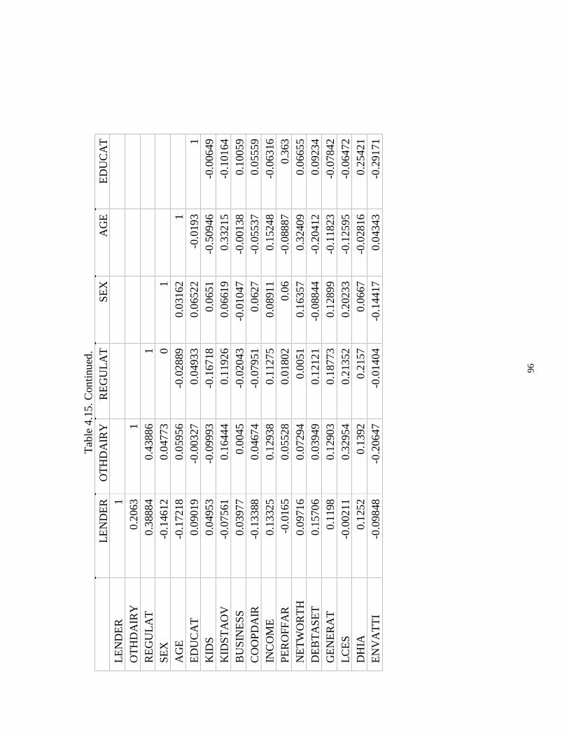
96
T
able
4.1
5. C
ontin
ued.
LE
ND
ER
O
TH
DA
IRY
R
EG
UL
AT
SE
X
AG
E
ED
UC
AT
L
EN
DE
R
1
OT
HD
AIR
Y
0.20
63
1
R
EG
UL
AT
0.
3888
4 0.
4388
6 1
S
EX
-0
.146
12
0.04
773
0 1
AG
E
-0.1
7218
0.
0595
6 -0
.028
89
0.03
162
1
ED
UC
AT
0.
0901
9 -0
.003
27
0.04
933
0.06
522
-0.0
193
1 K
IDS
0.04
953
-0.0
9993
-0
.167
18
0.06
51
-0.5
0946
-0
.006
49
KID
ST
AO
V
-0.0
7561
0.
1644
4 0.
1192
6 0.
0661
9 0.
3321
5 -0
.101
64
BU
SIN
ESS
0.
0397
7 0.
0045
-0
.020
43
-0.0
1047
-0
.001
38
0.10
059
CO
OPD
AIR
-0
.133
88
0.04
674
-0.0
7951
0.
0627
-0
.055
37
0.05
559
IN
CO
ME
0.
1332
5 0.
1293
8 0.
1127
5 0.
0891
1 0.
1524
8 -0
.063
16
PE
RO
FFA
R
-0.0
165
0.05
528
0.01
802
0.06
-0
.088
87
0.36
3 N
ET
WO
RT
H
0.09
716
0.07
294
0.00
51
0.16
357
0.32
409
0.06
655
DE
BT
ASE
T
0.15
706
0.03
949
0.12
121
-0.0
8844
-0
.204
12
0.09
234
GE
NE
RA
T
0.11
98
0.12
903
0.18
773
0.12
899
-0.1
1823
-0
.078
42
LC
ES
-0.0
0211
0.
3295
4 0.
2135
2 0.
2023
3 -0
.125
95
-0.0
6472
D
HIA
0.
1252
0.
1392
0.
2157
0.
0667
-0
.028
16
0.25
421
EN
VA
TT
I -0
.098
48
-0.2
0647
-0
.014
04
-0.1
4417
0.
0434
3 -0
.291
71

97
T
able
4.1
5. C
ontin
ued.
KID
S K
IDST
AO
V
BU
SIN
ESS
C
OO
PDA
IR
INC
OM
E
PER
OFF
AR
K
IDS
1
KID
ST
AO
V
-0.1
8344
1
BU
SIN
ESS
-0
.184
21
-0.1
6949
1
C
OO
PDA
IR
-0.0
0014
0.
0003
8 0.
0682
6 1
IN
CO
ME
-0
.030
37
0.05
63
-0.1
3824
-0
.070
41
1
PE
RO
FFA
R
-0.0
0307
-0
.029
05
0.01
729
0.13
322
0.13
454
1 N
ET
WO
RT
H
-0.1
5936
0.
0981
3 0.
1795
2 -0
.149
59
0.18
707
-0.0
5223
D
EB
TA
SET
0.
0115
0.
0011
1 -0
.049
99
0.08
261
0.00
182
0.18
424
GE
NE
RA
T
0.14
895
-0.0
4997
-0
.139
76
0.01
898
-0.0
2706
-0
.042
47
LC
ES
-0.0
5080
0.
0954
8 -0
.035
40
0.01
631
0.03
925
0.14
046
DH
IA
0.01
379
0.03
529
0.00
628
-0.0
7625
0.
0342
9 0.
1611
7 E
NV
AT
TI
-0.1
7696
-0
.061
15
0.02
668
0.05
367
-0.0
8897
-0
.162
8
Tab
le 4
.15.
Con
tinue
d.
N
ET
WO
RT
H
DE
BT
ASE
T
GE
NE
RA
T
LC
ES
DH
IA
EN
VA
TT
I N
ET
WO
RT
H
1 -0
.263
46
-0.0
462
0.13
436
0.27
947
-0.0
469
DE
BT
ASE
T
-0.2
6346
1
0.00
952
-0.0
0383
-0
.168
89
0.02
427
GE
NE
RA
T
-0.0
462
0.00
952
1 0.
1496
9 -0
.175
94
-0.0
2306
L
CE
S 0.
0038
7 0.
0631
2 0.
1548
7 1
0.03
337
0.16
879
DH
IA
0.27
947
-0.1
6889
-0
.175
94
0.15
202
1 -0
.204
09
EN
VA
TT
I -0
.046
9 0.
0242
7 -0
.023
06
0.06
932
-0.2
0409
1
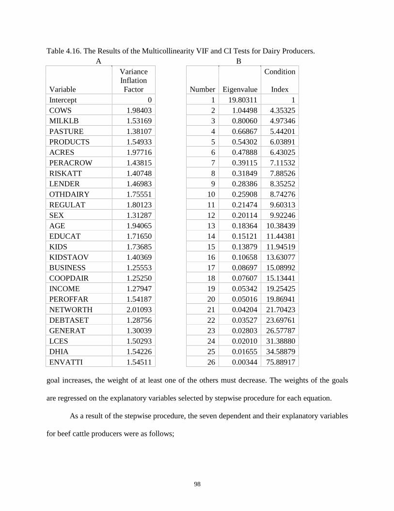
98
Table 4.16. The Results of the Multicollinearity VIF and CI Tests for Dairy Producers. A B
Variance Condition
Variable Inflation Factor Number Eigenvalue Index
Intercept 0 1 19.80311 1 COWS 1.98403 2 1.04498 4.35325 MILKLB 1.53169 3 0.80060 4.97346 PASTURE 1.38107 4 0.66867 5.44201 PRODUCTS 1.54933 5 0.54302 6.03891 ACRES 1.97716 6 0.47888 6.43025 PERACROW 1.43815 7 0.39115 7.11532 RISKATT 1.40748 8 0.31849 7.88526 LENDER 1.46983 9 0.28386 8.35252 OTHDAIRY 1.75551 10 0.25908 8.74276 REGULAT 1.80123 11 0.21474 9.60313 SEX 1.31287 12 0.20114 9.92246 AGE 1.94065 13 0.18364 10.38439 EDUCAT 1.71650 14 0.15121 11.44381 KIDS 1.73685 15 0.13879 11.94519 KIDSTAOV 1.40369 16 0.10658 13.63077 BUSINESS 1.25553 17 0.08697 15.08992 COOPDAIR 1.25250 18 0.07607 15.13441 INCOME 1.27947 19 0.05342 19.25425 PEROFFAR 1.54187 20 0.05016 19.86941 NETWORTH 2.01093 21 0.04204 21.70423 DEBTASET 1.28756 22 0.03527 23.69761 GENERAT 1.30039 23 0.02803 26.57787 LCES 1.50293 24 0.02010 31.38880 DHIA 1.54226 25 0.01655 34.58879 ENVATTI 1.54511 26 0.00344 75.88917
goal increases, the weight of at least one of the others must decrease. The weights of the goals
are regressed on the explanatory variables selected by stepwise procedure for each equation.
As a result of the stepwise procedure, the seven dependent and their explanatory variables
for beef cattle producers were as follows;

99
CONSFUZZ = f(ANIMALS, PUREBRED, MARKET, ACRES, PERACROW, KIDSTAOV,
BUSINESS, OTHBEEF, REGULAT, AGE, EDUCAT, KIDS, INCOME,
DEBTASET, ENVATTI).
PROFFUZZ = f(WEANING, ROTGRAZ, PRODUCTS, ACRES, KIDSTAOV, BUSINESS,
MEMBER, REGULAT, COUAGENT, INCOME, PEROFFAR).
SIZEFUZZ = f(ROTGRAZ, MARKET, PRODUCTS, KIDSTAOV, MEMBER, OTHBEEF,
AGE, KIDS, COUAGENT, INCOME, PEROFFAR, HENERAT, ENVATTI).
RISKFUZZ = f(ANIMALS, PUREBRED, CALTYPYR, MARKET, ACRES, KIDSTAOV,
RISKATT, LENDER, AGE, KIDS, COUAGENT, INCOME, PEROFFAR,
NETWORTH, DEBTASET, GENERAT).
NWORFUZZ = f(ANIMALS, PUREBRED, WEANING, PRODUCTS, MEMBER, RISKATT,
LENDER, OTHBEEF, REGULAT, AGE, KIDS, GENERAT, ENVATTI).
LEISFUZZ = f(ANIMALS, PUREBRED, ROTGRAZ, MARKET, PRODUCTS, ACRES,
KIDSTAOV, BUSINESS, MEMBER, RISKATT, LENDER, REGULAT,
KIDS, INCOME, PEROFFAR, NETWORTH, ENVATTI).
FAMIFUZZ = f(PUREBRED, WEANING, ROTGRAZ, MARKET, KIDSTAOV, RISKATT,
SEX, KIDS, PEROFFAR, NETWORTH, GENERAT)
The regression equations for dairy producers were:
CONSFUZZ = f(COWS, ACRES, RISKATT, LENDER, OTHDAIRY, REGULAT, AGE,
KIDS, KIDSTAOV, COOPDAIR, INCOME, PEROFFAR, DEBTASET,
LCES, DHIA, ENVATTI).

100
PROFFUZZ = f(MILKLB, PRODUCTS, PERACROW, RISKATT, LENDER, OTHDAIRY,
REGULAT, SEX, ADUCAT, KIDS, BUSINESS, COOPDAIR, INCOME,
NETWORTH, LCES, ENVATTI).
SIZEFUZZ = f(MILKLB, PASTURE, KIDSTAOV, COOPDAIR, INCOME, GENERAT,
ENVATTI).
RISKFUZZ = f(MILKLB, PASTURE, PRODUCTS, PERACROW, RISKATT, SEX, KIDS,
KIDSTAOV, COOPDAIR, PEROFFAR).
NWORFUZZ = f(PASTURE, PRODUCTS, ACRES, LENDER, OTHDAIRY, SEX, AGE,
EDUCAT, KIDSTAOV, COOPDAIR, INCOME, DEBTASET, GENERAT,
ENVATTI).
LEISFUZZ = f(COWS, MLIKLB, SEX, AGE, BUSINESS, INCOME, PEROFFAR,
NETWORTH, GENERAT, LCES, DHIA, ENVATTI).
FAMIFUZZ = F(COWS, MILKLB, PRODUCTS, ACRES, PERACROW, RISKATT,
LENDER, OTHDAIRY, SEX, AGE, KIDSTAOV, BUSINESS, COOPDAIR,
PEROFFAR, DEBTASET, GENERAT, LCES, DHIA).
A third analysis included both beef cattle and dairy producers. A dummy variable
(BF1DAIR0) was used that took the value of 1 if the observation was a beef cattle operation and
0 if dairy. The results of the stepwise explanatory selection are:
CONSFUZZ = f(ANIMALS, ACRES, PERACROW, LENDER, OTHPROD, AGE, EDUCAT,
KIDS, BUSINESS, INCOME, NETWORTH, DEBTASET, ENVATTI,
BF1DAIR0).
PROFFUZZ = f(ANIMALS, REGULAT, EDUCAT, KIDSTAOV, BUSINESS, PEROFFAR,
NETWORTH, ENVATTI, BF1DAIR0).
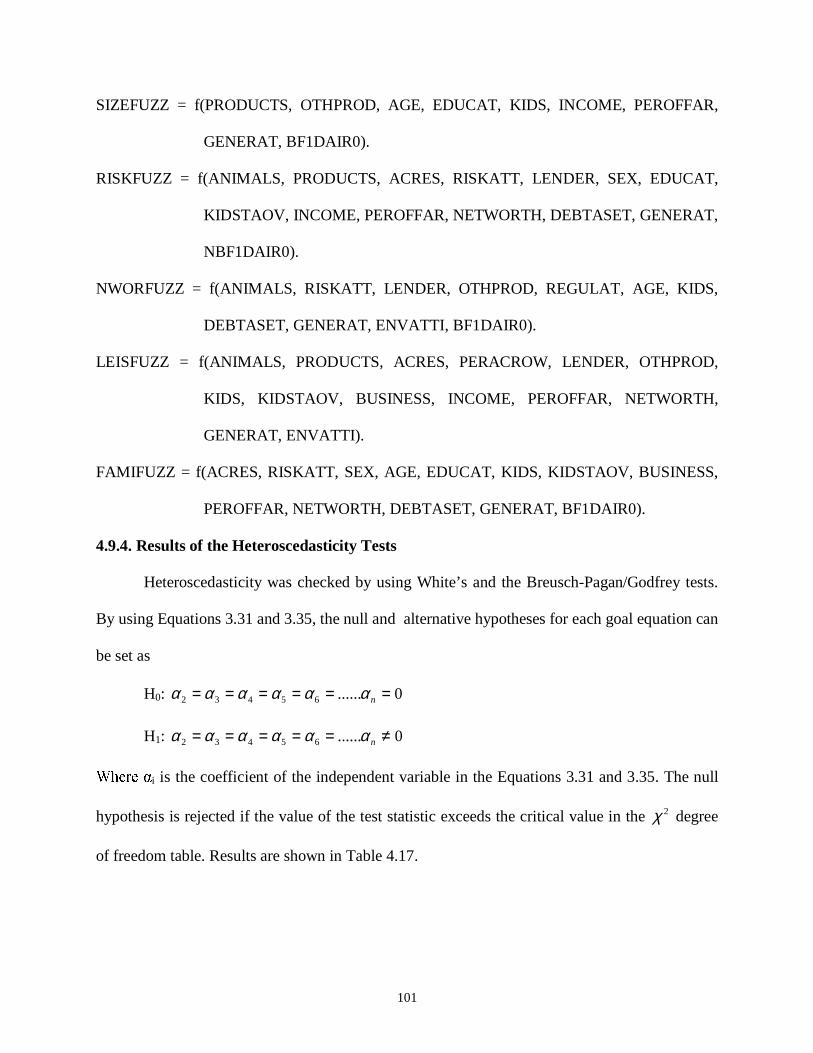
101
SIZEFUZZ = f(PRODUCTS, OTHPROD, AGE, EDUCAT, KIDS, INCOME, PEROFFAR,
GENERAT, BF1DAIR0).
RISKFUZZ = f(ANIMALS, PRODUCTS, ACRES, RISKATT, LENDER, SEX, EDUCAT,
KIDSTAOV, INCOME, PEROFFAR, NETWORTH, DEBTASET, GENERAT,
NBF1DAIR0).
NWORFUZZ = f(ANIMALS, RISKATT, LENDER, OTHPROD, REGULAT, AGE, KIDS,
DEBTASET, GENERAT, ENVATTI, BF1DAIR0).
LEISFUZZ = f(ANIMALS, PRODUCTS, ACRES, PERACROW, LENDER, OTHPROD,
KIDS, KIDSTAOV, BUSINESS, INCOME, PEROFFAR, NETWORTH,
GENERAT, ENVATTI).
FAMIFUZZ = f(ACRES, RISKATT, SEX, AGE, EDUCAT, KIDS, KIDSTAOV, BUSINESS,
PEROFFAR, NETWORTH, DEBTASET, GENERAT, BF1DAIR0).
4.9.4. Results of the Heteroscedasticity Tests
Heteroscedasticity was checked by using White’s and the Breusch-Pagan/Godfrey tests.
By using Equations 3.31 and 3.35, the null and alternative hypotheses for each goal equation can
be set as
H0: 0......65432 ====== nαααααα
H1: 0......65432 ≠===== nαααααα
������ i is the coefficient of the independent variable in the Equations 3.31 and 3.35. The null
hypothesis is rejected if the value of the test statistic exceeds the critical value in the 2χ degree
of freedom table. Results are shown in Table 4.17.

102
Table 4.17 . Heteroscedasticity Test Results for Beef Cattle and Dairy Variables.
Variables White’s Test Pr>ChiSq Breusch-
Pagan Pr>ChiSq Beef Cattle CONSFUZZ 178.60 0.0043 31.75 0.0070 PROFFUZZ 106.30 0.0053 20.04 0.0447 SIZEFUZZ 84.42 0.8518 15.66 0.2678 RISKFUZZ 226.30 <.0001 17.92 0.3288 NWORFUZZ 136.40 0.0130 20.62 0.0809 LEISFUZZ 158.10 0.6149 22.88 0.1533 FAMIFUZZ 60.37 0.8341 18.14 0.0785 Dairy CONSFUZZ 130.00 0.4587 11.75 0.8151 PROFFUZZ 130.00 0.4587 13.98 0.6003 SIZEFUZZ 37.34 0.2369 8.35 0.3029 RISKFUZZ 37.34 0.2369 6.04 0.8117 NWORFUZZ 117.40 0.2526 18.94 0.1674 LEISFUZZ 79.91 0.2447 15.32 0.1685 FAMIFUZZ 130.00 0.4587 15.92 0.5292
According to White’s test, there were heteroscedasticity problems in the Maintain and
Conserve land (CONSFUZZ), Maximize Profit (PROFFUZZ), Avoid Years of Loss / Low Profit
(RISKFUZZ), and Increase Net Worth (NWORFUZZ) regression equations in the beef cattle
analysis. On the other hand, according to the Breusch-Pagan/Godfrey test the CONSFUZZ and
PROFFUZZ regression equations had heteroscedasticity problems.
SUR equations are a form of the general error covariance statistical model which includes
heteroscedasticity and autocorrelation jointly. That is why seemingly unrelated regressions are
called error related regression equations. The generalized least squares estimation procedure
developed for solving heteroscedasticity problems is an appropriate rule in SUR equations. In
generalized least squares estimation, in order to solve the heteroscedasticity problem, two
common transformation procedures are used. In the first procedure, the statistical model is
transformed to one with a constant variance by dividing both sides of the equation by the square

103
root of the corresponding observation for the explanatory variable. In the second procedure, the
statistical model is transformed by dividing each variable of the equation by its variance. Both
transformations yield transformed error terms that have the same variance for all observations.
As a result of such transformations, the shape of the error terms is no longer heteroscedastic.
Ordinary least squares is applied to the transformed model for the estimation.
In logistic SUR equations there is not a heteroscedasticity problem with all of the
equations, and as explained above, because seemingly unrelated regression analysis uses
generalized least squares estimates, it is assumed that heteroscedasticity will not be a problem for
the system of equations (Judge et al., 1988). For the dairy analysis, there was no evidence of the
presence of heteroscedasticity in any of the regression equations.
4.9.5. Results of the Contemporaneous Correlation Test It was expected that the equation errors for each of the goals would be contemporaneously
correlated. In this case, the best system of equations that can be used is the seemingly unrelated
regression (SUR) model.
By applying Equation 3.141 to the cross model correlation from the regression analysis,
the values of the for beef cattle, dairy, and beef-dairy analyses were calculated. The values
for beef cattle, dairy, and beef-dairy were 422.02, 117.22, and 532.48, respectively. The degrees
of the freedom for each analysis was 21. The critical value 2χ for 21 degrees of freedom at the
0.05 significance level was 32.67. Since all values of the were greater than 32.67,
contemporaneous correlation was present in all three analyses. Thus, seemingly unrelated
regression was the most appropriate model for the estimation of the data.

104
4.10. The Results of Seemingly Unrelated Logistic Regression (SULR) Models Following are results of the SULR analyses for beef cattle producers, dairy producers,
and a combined analysis prior to examining results. It is worthwhile to recognize that if an
exogenous variable has a positive influence on one goal, it must have a negative influence on at
least one of the other goal. Thus, unexpected signs can occur on a particular variable largely
because producers of that description placed a counter balancing emphasis on another goal.
4.10.1. Results of the Seemingly Unrelated Logistic Regression Analysis for Beef Cattle Producers
The SULR model was used to estimate the effect of production characteristics,
producer’s risk attitude, social capital, environmental attitude, and producer and farm
characteristics on the goal structure of Louisiana beef cattle producers.
For the dependent variable Maintain and Conserve Land (CONSFUZZ), of the 16
independent variables, eight were significant. The variables PUREBRED, OTHBEEF, AGE,
INCOME, DEBTASET, and ENVATTI were significant at the 5 percent level, and variables
KIDSTAOV and BUSINESS were significant at the 10 percent level.
The Maximize Profit (PROFFUZZ) equation had 11 independent variables. Of the
eleven, REGULAT and COUAGENT were significant at the 5 percent level.
The Increase Farm Size (SIZEFUZZ) equation had 13 variables. Of the 13, the variable
INCOME was significant at the 5 percent level, and the variables ROTGRAZ, AGE,
COUAGENT, and GENERAT were significant at the 10 percent level.
Of the 16 independent variables, eight were significant in the Avoid Years of Loss / Low
Business (RISKFUZZ) equation. AGE, ANIMALS, and KIDSTAOV were significant at the 5
percent level. The variables which were significant at the 10 percent level were ACRES,
RISKATT, PEROFFAR, DEBTASET, and GENERAT.
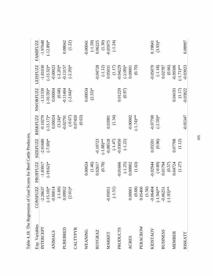
10
5
Tab
le 4
.18.
The
Reg
ress
ion
of G
oal S
core
s fo
r B
eef
Cat
tle P
rodu
cers
.
Exp
. Var
iabl
es
CO
NSF
UZ
Z
PRO
FFU
ZZ
S
IZE
FUZ
Z
RIS
KFU
ZZ
N
WO
RFU
ZZ
L
EIS
FUZ
Z
FAM
IFU
ZZ
IN
TE
RC
EPT
-2
.286
37
-1.8
3917
-2
.016
80
-0.1
0270
-1
.513
39
-1.8
1030
-1
.976
48
(-
15.1
0)*
(-19
.62)
* (-
7.69
)*
(-13
.17)
* (-
10.5
9)*
(-13
.32)
* (-
12.8
9)*
AN
IMA
LS
-0.0
0014
0.
0002
4 0.
0000
4 -0
.000
23
(-1.
60)
(3.2
4)*
(0.6
8)
(-2.
20)*
PUR
EB
RE
D
0.09
952
-0.0
2791
-0
.114
04
-0.1
3157
0.
0804
2
(2.0
1)*
(-0.
67)
(-2.
64)*
(-
2.29
)*
(1.2
2)
CA
LT
YPY
R
0.
0745
0
(0.6
3)
W
EA
NIN
G
0.
0002
4
0.
0003
4
-0.0
0041
(1
.46)
(2
.33)
*
(-1.
59)
RO
TG
RA
Z
0.
0261
7 -0
.107
23
-0.0
4728
0.
0622
5
(0
.78)
(-
1.88
)**
(-1.
12)
(1.3
0)
MA
RK
ET
-0
.050
51
-0
.085
18
0.03
981
0.
0503
1 -0
.059
75
(-
1.51
)
(-1.
47)
(1.3
4)
(1
.17)
(-
1.24
) PR
OD
UC
TS
-0
.016
66
-0.0
3050
0.01
229
-0.0
4229
(-1.
25)
(-1.
22)
(0
.97)
(-
2.09
)*
A
CR
ES
0.00
001
0.00
002
-0
.000
02
0.
0000
1
(0
.68)
(1
.63)
(-1.
74)*
*
(0.7
0)
PE
RA
CR
OW
0.
0540
0
(1.5
6)
KID
STA
OV
-0
.064
04
-0.0
2944
0.
0559
1 -0
.077
00
-0
.050
70
0.19
841
(-
1.94
)**
(-0.
89)
(0.9
6)
(-2.
59)*
(-1.
18)
(3.9
3)*
BU
SIN
ESS
-0
.062
51
0.01
794
0.
0278
7
(-
1.93
)**
(0.5
7)
(0
.66)
ME
MB
ER
0.04
724
0.07
708
0.
0419
3 -0
.093
06
(1
.27)
(1
.12)
(1.1
7)
(-1.
71)*
*
RIS
KA
TT
-0.0
5347
-0
.038
22
-0.0
3923
0.
0899
7

10
6
Tab
le 4
.18
Con
tinue
d.
(-1.
90)*
* (-
1.33
) (-
1.02
) (2
.05)
* L
EN
DE
R
0.
0188
8 0.
0237
5 -0
.024
12
(1
.52)
(1
.65)
**
(-1.
29)
O
TH
BE
EF
0.04
368
0.
0473
3
-0.0
7349
(1.9
5)*
(1
.53)
(-3.
45)*
R
EG
UL
AT
-0
.014
92
0.03
085
0.04
244
-0.0
2235
(-
0.76
) (2
.02)
*
(2
.25)
* (-
0.98
)
SEX
0.
1849
6
(2.7
1)*
AG
E
0.00
659
-0
.004
69
0.00
338
-0.0
0283
(4.2
7)*
(-
1.85
)**
(2.4
8)*
(-2.
15)*
E
DU
CA
T
0.01
010
(0
.97)
K
IDS
0.01
668
-0
.025
15
0.01
076
-0.0
3749
0.
0461
7 0.
0395
6
(0.9
3)
(-
0.83
) (0
.70)
(-
2.34
)*
(2.3
3)*
(1.8
4)**
C
OU
AG
EN
T
-0
.050
84
0.08
638
0.02
719
(-
1.95
)*
(1.6
9)**
(1
.05)
INC
OM
E
0.02
371
-0.0
0771
0.
0381
6 -0
.012
26
-0
.022
81
(2.8
9)*
(-1.
04)
(2.7
3)*
(-1.
41)
(-
1.83
)**
PE
RO
FFA
R
-0
.012
38
0.01
535
0.01
412
-0
.014
32
-0.0
0683
(-
1.49
) (1
.04)
(1
.87)
**
(-
1.34
) (-
0.57
) N
ET
WO
RT
H
-0
.008
80
0.
0505
8 -0
.037
15
(-0.
77)
(3
.35)
* (-
2.56
)*
DE
BT
ASE
T
-0.0
3078
0.
0273
8
(-
2.01
)*
(1.9
4)**
GE
NE
RA
T
-0.0
4142
0.
0220
4 -0
.010
10
0.
0373
8
(-1.
78)*
* (1
.75)
**
(-0.
84)
(1
.98)
* E
NV
AT
TI
0.04
942
-0
.035
67
-0
.067
00
0.02
951
(2.0
5)*
(-
0.89
)
(-3.
02)*
(0
.98)
R2
0.11
0.
03
0.07
0.
08
0.09
0.
08
0.09
Sy
stem
R2 =
0.08
t -
val
ues
in p
aren
thes
is
* =
sig
nifi
cant
at .
05
** =
Sig
nifi
cant
at .
10
R2 =
0.08

107
For the Increase Net Worth (NWORFUZZ) equation, there were 13 independent
variables. PUREBRED, WEANING, OTHBEEF, REGULAT, AGE, KIDS, and ENVATTI were
significant at the 5 percent level, and variable LENDER was significant at the 10 percent level.
Have Time for Other Activities (LEISFUZZ) had 17 independent variables and seven
were significant. ANIMALS, PUREBRED, PRODUCTS, KIDS, and NETWORTH were
significant at the 5 percent level, and variables MEMBER, and INCOME were significant at the
10 percent level.
The last regression equation for beef cattle producers’ goal structure was Have Family
Involved in Agriculture (FAMIFUZZ). The equation included 11 independent variables.
Variables KIDSTAOV, RISKATT, SEX, NETWORTH, and GENERAT were significant at the
5 percent level, and KIDS was significant at the 10 percent level.
The discussion of signs and variable significance will proceed by independent variable,
rather than by dependent variable. Thus, I will start with ANIMALS and proceed.
The positive relationship between the number of animals that the beef cattle producer had
(ANIMALS) and the goal of Avoid Years of Loss / Low Profit (RISKFUZZ) was of the expected
positive sign. This is consistent with discussion by Gillespie et al., which made the point that as
the size of the operation increases, greater risk associated with being larger and likely less
diversified occurs. Thus, these producers are likely to have a greater concern for risk. On the
other hand, as the number of the animals increases, the producer needs to spend more time on the
operation. Thus, the negative correlation between ANIMALS and LEISFUZZ was also expected.
The results of the regression show that PUREBRED had a positive effect on Maintain
and Conserve Land and a negative effect on Increase Net Worth and Have Time for Other
Activities.
108
As expected, the average weaning weight of calves (WEANING) was positively
correlated with Maximize Profit. However, the effect of WEANING was not significant. On the
other hand, there was a positive correlation between WEANING and Increase Net Worth.
According to the stepwise selection procedure, ROTGRAZ did not have an expected
significant effect on Maintain and Conserve Land, and was not included in the equation.
ROTGRAZ had an expected negative correlation with Increase Farm Size. As discussed by
Bettz, since the system requires intensive management and capital investment, labor availability
is likely to constrain rotational grazers from greatly expanding their operations.
MARKET was not included in Maximize Profit equation. In addition of this, the variable
had no significant effect in the other equations.
The PRODUCTS variable did not have a significant effect on Avoid Years of Loss / Low
Profit even at the .50 percent in the selection procedure. That is why the variable was not
included in Avoid Years of Loss / Low Profit equation. On the other hand, PRODUCTS had an
expected negative effect on Have Time for Other Activities. As the number of enterprises
increases, the time requirement for management increases and the time available for leisure is
likely to decrease.
ACRES had a positive effect on Have Time for Other Activities. However, the effect was
insignificant. The variable had a negative effect on Avoid Years of Loss / Low Profit. On the
other hand, PERACROW had the expected positive effect on Maintain and Conserve Land. This
is consistent with discussion of Smith and Capstick in the case that the land owners have an
incentive to conduct long-term maintenance tasks on their property.

109
The variable KIDSTAOV had an expected positive sign on Have Family Involved in
Agriculture, and an unexpected negative sign on Maintain and Conserve Land. The variable had
a negative effect on Avoid Years of Loss / Low Profit.
BUSINESS had a negative effect on Maintain and Conserve Land. Thus, there is a
positive relationship between shared ownership and the conservation goal. This raises the
interesting question of whether property is better maintained under joint ownership.
The expected positive correlation between MEMBER and Maximize Profit was not
significant. The variable was not included in the RISKFUZZ equation. On the other hand, there
was a negative correlation between MEMBER and Have Time for Other Activities: the producer
who is a member of a market alliance is likely to place more emphasis on financial than leisure
goals.
RISKATT had an expected negative effect on Avoid Years of Loss / Low Profit. The
variable also had a positive effect on Have Family Involved in Agriculture.
LENDER had an expected positive effect on Increase Net Worth. A social relationship
with the lender is considered valuable by producers who desire to increase their wealth.
OTHBEEF had positive and negative effects on Maintain and Conserve Land and
Increase Net Worth, respectively. The result suggests that producers who value relationships
with neighboring beef cattle producers are likely to place more emphasis on maintaining their
land, and less emphasis on increasing wealth.
The degree of importance of the farmers’ relationship with regulatory agencies had an
expected positive effect on Maximize Profit and an unexpected negative effect on Maintain and
Conserve Land. The variable also had a positive effect on Increase Net Worth. Regulatory
agency personnel can provide valuable information as to rules and regulations prior to the

110
expansion of facilities. Moreover, funding is available via the federal government for
implementation of conservation practices through the Conservation Reserve Program and the
Environmental Quality Incentives Program. Such programs can be economically advantageous to
producers.
Male producers placed a greater weight on Have Family Involved in Agriculture than did
female producers.
The relationship between AGE and Avoid Years of Loss / Low Profit was positive as
expected. This means that the older producers were more concerned about avoiding financial
losses and / or low returns. The negative effect between AGE and Increase Net Worth was
expected. In addition to these, there were positive and negative correlations between AGE and
Maintain and Conserve Land, and AGE and Increase Farm Size, respectively. As discussed by
Klemme, farms are classified into three types, turnkey, established, and debt-free, according to
their planning horizon. The owners of turnkey and established farms are relatively younger and
they tend to increase their farm size. On the other hand, the owner of debt-free farms are
relatively older and likely not interested in new investment and increasing the size of their
operations.
The effect of EDUCAT was non-significant in the any of the equations.
As expected, KIDS had a positive effect on both Have Time for Other Activities and
Have Family Involved in Agriculture. This is consistent with the findings of both Van Kooten et
al., and Smith and Capstick. On the other hand, there was a negative relationship between KIDS
and Increase Net Worth, leading to the conclusion that goals other than increasing wealth
became more important when the producer had a child in the household.

111
The negative correlation between COUAGENT and Maximize Profit was not expected.
On the other hand, the variable had a positive effect on Increase Farm Size.
The relationship between INCOME and Have Time for Other Activities was negative. On
the other hand, the INCOME variable had a positive effect on Maintain and Conserve Land and a
negative effect on Increase Farm Size. It is likely that higher income producers are part-time
farmers who own land and enjoy working with cattle, rather than being concerned with the
financial aspects of the operation. Thus, maintaining and conserving the limited land via cattle
production is how these producers spend their leisure time.
The positive correlation between PEROFFAR and Avoid Years of Loss / Low Profit was
expected. Having an off-farm job is a form of diversification, which is risk reducing. Thus, the
producer may be diversifying because he wants to avoid years of loss.
There was a positive relationship between NETWORTH and Have Time for Other
Activities, and a negative relationship between NETWORTH and Have Family Involved in
Agriculture. These results are consistent with each other in the sense that, as the producer’s net
worth increases, instead of having his family involved in agriculture, the producer desires to
spend more time for leisure.
The positive correlation between DEBTASET and Avoid Years of Loss / Low Profit was
expected. On the other hand, there was a negative relationship between DEBTASET and
Maintain and Conserve Land. The result suggests that, if the producer has higher debt relative to
assets, he will be more concerned about the short run risk of going out of business rather than
long-run goals associated with conservation.
GENERAT had the expected positive sign on Have Family Involved in Agriculture. On
the other hand, there was a negative relationship between GENERAT and Increase Farm Size
112
and a positive relationship between GENERAT and Avoid Years of Loss / Low Profit. The
results suggest that as the generation on the farm increases, the producer becomes more
concerned with not being forced out of business, and more concerned with having the family
being involved in agriculture, possibly due to family tradition.
The positive correlation between ENVATTI and Maintain and Conserve Land was
expected. There was also a negative relationship between ENVATTI and Increase Farm Size.
The result suggests that producers who are more concerned about the environment are less likely
to place an emphasis on becoming larger, possibly because increasing span of control takes away
from the ability to maintain the property at the desired level.
The size of the system R2 is 0.08. The value seems to be very low. Researchers have
found that “the size of R2 and 2R are poor specification indicators since correctly specified
models can have “low” R2 values and misspecified models often have “high” R2 values (McGuirk
and Driscoll, 1995). This means that the value of R2 may not be a consistent measure of the
goodness of fit. The lower size of R2 does not indicate that the beef cattle model is misspecified.
4.10.2. Results of the Seemingly Unrelated Logistic Regression Analysis for Dairy Producers
As with the beef cattle analysis, the logistic SUR model was used to estimate the effect of
independent variables on the goal structure of Louisiana dairy producers. The seven goals were
regressed on 25 explanatory variables. The results are given in Table 4.19.
For the dependent variable CONSFUZZ, of the 17 independent variables, 6 were
significant. The variables KIDSTAOV, LCES, DHIA and ENVATTI were significant at the 5
percent level, and variables OTHDAIRY and PEROFFFAR were significant at the 10 percent
level.

113
The PROFFUZZ equation had 16 independent variables. Of the 16, RISKATT, SEX,
BUSINESS, and ENVATTI were significant at the 5 percent level and variables EDUCAT,
INCOME, and LCES were significant at the 10 percent level.
The SIZEFUZZ equation had 7 variables. Of the 7, the variable COOPDAIR was
significant at the 5 percent level, and the variables PASTURE and ENVATTI were significant at
the 10 percent level.
Of the 10 variables in the RISKFUZZ equation, 5 variables were significant. MILKLB,
KIDS, and COOPDAIR were significant at the 5 percent level. The variables which were
significant at the 10 percent level were KIDSTAOV and PEROFFAR.
For the NWORFUZZ equation, there were 14 independent variables. PRODUCTS,
OTHDAIRY, AGE, and ENVATTI were significant at the 5 percent level, and LENDER was
significant at the 10 percent level.
LEISFUZZ had 11 independent variables and 3 of them were significant. The 3
significant variables at the 5 percent level were COWS, NETWORTH and LCES.
The last regression equation for dairy producers was FAMIFUZZ. The equation included
17 independent variables. Variables ACRES, AGE, BUSINESS and PEROFFAR were
significant at the 5 percent level.
Like the ANIMALS variable in the beef cattle model, the relationship between the
number of dairy cows (COWS) and Have Time for Other Activities was of the expected negative
sign.
There was a negative relationship between MILKLB and Avoid Years of Loss / Low
profit. It is possible that as the amount of milk per cow increases, the producer is more confident

11
4
Tab
le 4
.19.
The
Reg
ress
ion
of G
oal S
core
s fo
r D
airy
Pro
duce
rs.
Exp
. Var
iabl
es
CO
NSF
UZ
Z
PRO
FFU
ZZ
S
IZE
FUZ
Z
RIS
KFU
ZZ
N
WO
RFU
ZZ
L
EIS
FUZ
Z
FAM
IFU
ZZ
IN
TE
RC
EPT
-2
.374
09
-1.7
3286
-2
.541
90
-1.0
8359
-1
.644
32
-2.3
9172
-1
.407
81
(-
6.51
)*
(-7.
73)*
(-
4.46
)*
(-4.
95)*
(-
5.72
)*
(-7.
45)*
(-
3.22
)*
CO
WS
0.00
0281
0.
0002
02
-0
.001
25
0.00
0749
(0.6
5)
(0.7
7)
(-
2.89
)*
(1.3
5)
MIL
KL
B
-0.0
0004
-0
.000
03
0.
0000
21
0.00
001
(-
1.50
) (-
2.68
)*
(1
.27)
(0
.46)
PA
ST
UR
E
-0.3
6145
0.
1452
64
-0.0
7748
(-1.
69)*
* (1
.52)
(-
0.92
)
PR
OD
UC
TS
0.02
1298
-0
.029
56
0.
0306
4 -0
.054
40
0.
0481
33
(0
.66)
(-
1.43
)
(1.3
6)
(-2.
21)*
(1.0
7)
AC
RE
S 0.
0001
66
0.
0001
26
-0
.000
41
(1
.32)
(1.4
0)
(-
2.62
)*
PER
AC
RO
W
0.
0954
94
-0
.072
36
-0.1
0490
(1
.42)
(-0.
98)
(-0.
82)
RIS
KA
TT
-0
.115
54
0.10
4991
0.07
9903
-0
.121
80
(-
1.56
) (2
.04)
*
(1.4
3)
(-1.
16)
LE
ND
ER
-0
.069
51
0.04
0961
0.
0705
17
0.06
9422
-0
.057
18
(-
1.19
) (1
.09)
(1
.67)
**
(1.1
9)
(-0.
81)
OT
HD
AIR
Y
0.10
4594
-0
.057
77
-0.1
0016
0.07
7431
(1.9
0)**
(-
1.60
)
(-
2.61
)*
(1
.12)
R
EG
UL
AT
0.
0404
36
0.03
7662
(0
.97)
(1
.26)
SEX
0.17
9607
-0.0
7944
0.
0796
36
-0.1
6464
-0
.153
86
(2.3
5)*
(-
0.92
) (0
.97)
(-
1.31
) (-
1.00
) A
GE
0.
0041
61
0.
0048
75
-0
.008
07
(1
.21)
(2.0
3)*
(-
2.02
)*

11
5
Tab
le 4
.19
Con
tinue
d.
ED
UC
AT
0.03
2849
-0
.024
60
(1.7
1)**
(-
1.14
)
K
IDS
0.04
0142
0.
0187
92
-0
.058
82
(1.4
2)
(0.9
9)
(-
2.86
)*
K
IDST
AO
V
0.18
5440
-0.1
7782
-0
.115
13
-0.0
6754
-0
.079
57
0.15
5841
(2.1
9)*
(-
1.35
) (-
1.89
)**
(-1.
09)
(-0.
89)
(1.4
3)
BU
SIN
ESS
0.13
1800
-0
.164
98
(3.1
6)*
(-2.
24)*
C
OO
PDA
IR
-0.1
0751
0.
0409
40
0.45
5241
-0
.195
50
0.10
7613
0.
1042
56
(-1.
20)
(0.7
2)
(2.9
3)*
(-2.
88)*
(1
.61)
(0
.98)
INC
OM
E
-0.0
2012
0.
0172
06
0.03
0026
0.01
4691
-0
.029
51
(-1.
31)
(1.7
7)**
(1
.21)
(1.3
0)
(-1.
63)
PE
RO
FFA
R
0.04
3068
0.
0321
26
-0
.040
77
-0.0
7670
(1.8
8)**
(1
.84)
**
(-
1.61
) (-
2.60
)*
NE
TW
OR
TH
-0.0
3187
0.07
5944
(-1.
63)
(2
.47)
*
DE
BT
ASE
T
-0.0
3710
0.02
1198
-0.0
4915
(-1.
25)
(0
.94)
(-1.
32)
GE
NE
RA
T
-0.0
1237
-0.0
2259
-0.0
1868
(-0.
26)
(-
1.00
)
(-0.
50)
LC
ES
-0.1
8737
-0
.089
55
0.
1996
55
0.15
3762
(-2.
35)*
(-
1.67
)**
(2
.45)
* (1
.53)
D
HIA
-0
.194
51
0.09
2917
0.
1378
63
(-
2.88
)*
(1.2
7)
(1.6
3)
EN
VA
TT
I 0.
1369
35
-0.0
8345
0.
1643
41
-0
.089
74
(2
.41)
* (-
2.33
)*
(1.9
7)**
(-2.
15)*
R
2 0.
22
0.28
0.
13
0.16
0.
17
0.18
0.
22
Syst
em R
2 =
0.1
9
t –
val
ues
in p
aren
thes
is
* =
sig
nifi
cant
at .
05
** =
Sig
nifi
cant
at .
10

116
that he or she will not have as many years of loss / low profit.
A positive correlation was expected between PASTURE and Maintain and Conserve
Land. However, according to the stepwise selection procedure, the variable was not significant
enough to be included in the regression analysis. On the other hand, there was a negative
correlation between PASTURE and Increase Farm Size. Pasture based dairy operations are more
constrained by land availability than free-stall based operations.
Unlike the beef cattle analysis, PRODUCTS had the expected positive effect on Avoid
Years of Loss / Low Profit, but it was insignificant. On the other hand, PRODUCTS had a
negative effect on Increase Net Worth.
The amount of land used in the operation (ACRES), had a negative effect on the Have
Family Involved in Agriculture. Thus, larger scale producers placed less emphasis on having the
family involved on the farm than other goals.
RISKATT had a positive effect on Maximize Profit. This correlation is consistent with
Robison and Barry: “a risky investment or enterprise must yield an expected return high enough
(compared to a risk free investment) to compensate the risk-averse decision maker for accepting
the risk.”
As with the beef cattle model, LENDER had an expected positive effect on Increase Net
Worth. As with the beef cattle model, OTHDAIRY had a positive effect on Maintain and
Conserve Land, and a negative effect on Increase Net Worth. In the case of gender, the male
dairy farmers were more profit oriented, while the male beef cattle farmers were more interested
in having the family involved in agriculture..
The relationship between AGE and Increase Net Worth was of the expected positive sign.
Thus, the older producers placed more value on Increase Net Worth. This is the opposite of the

117
beef cattle result. On the other hand, there was a negative correlation between AGE and Have
Family Involved in Agriculture.
As expected, EDUCAT had a positive effect on Maximize Profit.
The positive effect of KIDS on Maintain and Conserve Land was expected; however, it is
insignificant. On the other hand, KIDS had an unexpected negative effect on Avoid Years of
Loss / Low Profit.
Unlike beef cattle producers, the variable KIDSTAOV had the expected positive effect
on the Maintain and Conserve Land, and an unexpected negative sign on Avoid Years of Loss /
Low Profit. BUSINESS had a positive effect on Maximize Profit and a negative effect on Have
Family Involved in Agriculture. Thus, dairy producers involved in joint ownership firms placed
greater emphasis on Maximize Profit and less on Having the Family Involved in Agriculture.
COOPDAIR had a surprisingly negative effect on Avoid Years of Loss / Low Profit, and
a positive effect on Increase Farm Size. The expected positive correlation between COOPDAIR
and Maximize Profit was not significant.
INCOME had a negative effect on Have Time for Other Activities; however, it was
insignificant. The significant relationship between INCOME and Maximize Profit was positive
as expected.
As with beef cattle producers, the correlation between PEROFFAR and Avoid Years of
Loss / Low Profit was of the expected positive sign. PEROFFAR had a negative effect on Have
Family Involved in Agriculture, and a positive effect on Maintain and Conserve Land. Greater
time spent in an off farm job leaves less time for family oriented goals. However, as the reliance
on the farm as a source of income decreases, more emphasis may be placed on preserving land
for future generations, rather than short-run returns.

118
A positive correlation between NETWORTH and Increase Net Worth was expected.
However, in the stepwise selection procedure, the variable did not have a significant effect. On
the other hand, as with the beef cattle analysis, there was a positive relationship between
NETWORTH and Have Time for Other Activities. This result suggests that the producers who
have greater net worth place a greater emphasis on leisure.
The effect of LCES on Maintain and Conserve Land and Maximize Profit were
surprisingly negative. On the other hand, the variable had an positive effect on Have Time for
Other Activities.
In the stepwise selection procedure, DHIA was not significant enough to be included in
the Maximize Profit and Avoid Years of Loss / Low Profit equations. There was a significant
negative correlation between DHIA and Maintain and Conserve Land.
The positive correlation between ENVATTI and Maintain and Conserve Land was
expected. Thus, the more environmentally minded producer placed greater emphasis on Maintain
and Conserve Land. On the other hand, there were negative relationships between ENVATTI
and Maximize Profit and Increase Net Worth and a positive relationship with Increase Farm
Size.
For the dairy analysis the size of the system R2 is 0.19. The value is low but higher than
for the beef cattle analysis. As discussed previously with respect to the beef cattle model, the
lower size of R2 does not indicate that the dairy model is either misspecified or better specified
that the beef cattle model.
4.10.3. Results of the Combined Seemingly Unrelated Logistic Regression Analysis for Beef Cattle and Dairy Producers
For the combined analysis, the beef cattle and dairy data were combined into one dataset
and the logistic SUR model was used to estimate the effects of independent variables on goal

119
structure. The selection of independent variables for each equation was conducted by using the
stepwise procedure, as in the other analyses. Results of the estimations are given in Table 4.20.
Note that the variables ANIMALS and COWS were combined and the new variable for both
dairy and beef cattle producers was called ANIMALS. OTHBEEF and OTHDAIRY variables
were combined and the new variable was called OTHPROD.
For the dependent variable Maintain and Conserve Land, of the 14 independent variables, 6 were
significant. The variables ANIMALS, OTHPROD, AGE, and ENVATTI were significant at the
5 percent level, and variables DEBTASET and BF1DAIR0 were significant at the 10 percent
level.
The Maximize Profit equation had 9 independent variables. Of the 9, ANIMALS,
REGULAT and BF1DAIR0 were significant at the 5 percent level.The Increase Farm Size
equation had 9 variables. Of the 9, AGE, INCOME and BF1DAIR0 were significant at the 5
percent level, and PRODUCTS and GENERAT were significant at the 10 percent level.
Of the 15 variables in Avoid Years of Loss / Low Profit equation 7 were significant.
ANIMALS, AGE, KIDSTAOV, PEROFFAR, BF1DAIR0 were significant at the 5 percent level.
Variables significant at the 10 percent level were RISKATT and LENDER.
For the Increase Net Worth equation, there were 11 independent variables. LENDER,
OTHBEEF, KIDS, ENVATTI and BF1DA5R0 were significant at the 5 percent level.
Have Time for Other Activities had 14 independent variables and seven of them were significant.
The significance level was at the 5 percent for variables ANIMALS, PRODUCTS, KIDS,
KIDSTAOV, INCOME, PEROFFAR, and NETWORTH.
The Have Family Involved in Agriculture equation included 13 independent variables.
The variables SEX, KIDSTAOV, and BF1DAIR0 were significant at the 5 percent level, and

12
0
Tab
le 4
.20.
The
Reg
ress
ion
of G
oal S
core
s fo
r B
eef
Cat
tle a
nd D
airy
Pro
duce
rs
Exp
lana
tory
V
aria
bles
C
ON
SFU
ZZ
PR
OFF
UZ
Z
SIZ
EFU
ZZ
R
ISK
FUZ
Z
NW
OR
FUZ
Z
LE
ISFU
ZZ
FA
MIF
UZ
Z
INT
ER
CE
PT
-2.4
5761
-1
.653
47
-2.2
3636
-1
.859
45
-1.3
9035
-1
.925
34
-1.8
0958
(-16
.49)
* (-
18.4
6)*
(-11
.68)
* (-
17.6
)*
(-11
.48)
* (-
14.3
6)*
(-10
.21)
* A
NIM
AL
S -0
.000
19
0.00
011
0.
0002
4 0.
0000
7 -0
.000
31
(-2.
14)*
(2
.06)
*
(3.3
1)*
(1.3
9)
(-2.
86)*
PRO
DU
CT
S
-0
.039
14
0.00
951
-0
.043
20
(-1.
68)*
* (0
.83)
(-2.
72)*
AC
RE
S 0.
0000
2
-0
.000
02
0.
0000
3 -0
.000
02
(-
1.08
)
(-
1.53
)
(1.4
1)
(-1.
08)
PER
AC
RO
W
0.04
631
-0.0
3399
(1
.28)
(-
0.79
)
RIS
KA
TT
-0.0
4139
-0
.039
24
0.
0411
9
(-
1.66
)**
(-1.
56)
(1
.01)
L
EN
DE
R
-0.0
1300
0.
0228
7 0.
0329
4 -0
.017
61
(-0.
81)
(1.8
9)**
(2
.29)
* (-
0.97
)
OT
HPR
OD
0.
0449
4
0.04
056
-0
.059
63
-0.0
2020
(2
.26)
*
(1.3
2)
(-
3.2)
* (-
0.84
)
RE
GU
LA
T
0.
0282
4
0.
0199
9
(2
.27)
*
(1
.35)
SE
X
-0
.050
89
0.13
194
(-1.
21)
(2.0
2)*
AG
E
0.00
690
-0
.005
33
0.00
282
-0.0
0131
-0.0
0332
(4.7
3)*
(-
2.30
)*
(2.4
9)*
(-1.
06)
(-
1.68
)**

NOTE TO USERS
Page(s) missing in number only; text follows. The manuscript was microfilmed as received.
121-122
This reproduction is the best copy available.
UMI®

12
3
Tab
le 4
.20
Con
tinue
d.
ED
UC
AT
0.
0107
2 0.
0121
0 -0
.021
75
0.00
964
-0.0
1798
(0.9
5)
(1.1
6)
(-1.
11)
(0.9
5)
(1.0
3)
KID
S 0.
0228
5
-0.0
3461
-0.0
3005
0.
0351
8 0.
0255
3
(1.4
2)
(-
1.32
)
(-2.
17)*
(2
.05)
* (1
.24)
K
IDST
AO
V
-0
.030
76
-0
.085
22
-0
.071
76
0.19
817
(-1.
06)
(-
3.27
)*
(-
1.97
)*
(4.4
6)*
BU
SIN
ESS
-0
.046
40
0.04
482
0.
0514
1 -0
.061
60
(-
1.50
) (1
.53)
(1.3
8)
(-1.
37)
INC
OM
E
0.01
051
0.
0331
4 -0
.009
42
-0
.024
84
(1.3
2)
(2
.62)
* (-
1.34
)
(-2.
48)*
PER
OFF
AR
-0.0
0763
0.
0139
1 0.
0155
0
-0.0
1929
-0
.012
38
(-1.
03)
(0.9
8)
(2.1
6)*
(-
2.13
)*
(-1.
06)
NE
TW
OR
TH
0.
0136
0 -0
.012
99
-0
.012
71
0.
0592
8 -0
.028
65
(1
.13)
(-
1.32
)
(-1.
23)
(4
.03)
* (-
1.84
)**
DE
BT
ASE
T
-0.0
2661
0.
0206
6 0.
0111
4
-0.0
2959
(-1.
71)*
*
(1
.63)
(0
.83)
(-1.
43)
GE
NE
RA
T
-0.0
4225
0.
0171
2 -0
.007
91
0.01
253
0.01
537
(-
1.83
)**
(1.5
0)
(-0.
71)
(0.7
8)
(0.8
7)
EN
VA
TT
I 0.
0612
1 -0
.014
49
-0.0
7375
0.
0389
8
(2
.66)
* (-
0.75
)
(-
3.7)
* (1
.42)
BF1
DA
IR0
0.06
794
-0.1
0673
0.
2279
0 -0
.096
87
-0.0
7284
0.13
809
(1
.77)
**
(-3.
1)*
(3.4
3)*
(-2.
75)*
(-
2.25
)*
(2
.26)
* R
2
0.10
0.
05
0.06
0.
07
0.07
0.
07
0.07
Sy
stem
R2 =
0.0
7
t - v
alue
s in
par
enth
esis
*
= s
igni
fica
nt a
t .05
**
= S
igni
fica
nt a
t .10

124
variables AGE and NETWORTH were significant at the 10 percent level.
Generally, the signs of the significant variables were the same as in the beef cattle and
dairy models. Thus, only the effect of BF1DAIR0 will be discussed here.
As a result of the stepwise procedure, BF1DAIR0 appeared in six equations and had
significant effects on the independent variables. BF1DAIR0 did not appear in the Have Time
for Other Activities equation.
The results of the logistic SUR model were consistent with results of the fuzzy pair-
wise comparison. In the fuzzy pair-wise comparison, the dairy producers placed more
emphasis on the profit related goals. By examining the results of the logistic SUR, we see
that dairy producers placed greater emphasis on Maximize Profit, Avoid Years of Loss / Low
Profit, and Increase Net Worth. These goals were the most important three goals for dairy
producers in the fuzzy procedure.
In the case of beef producers, as discussed by Lamb and Beshear, the difference
between goal structures of beef cattle and dairy producers is likely due to fact that many
producers are “hobby farmers,” and economic profit is not the primary goal. According to the
fuzzy pair-wise procedure results, the most important goal of beef cattle producers was
Maintain and Conserve Land. This is consistent with the result of the logistic SUR regression
analysis.
The size of the system R2 is 0.07, which is the lowest value among the three models.
As discussed by McGuirk and Driscoll, this does not indicate that the model is misspecified.

125
CHAPTER 5. SUMMARY AND CONCLUSIONS
5.1. Summary and Conclusions
Much of the success of a farm depends on the quality of decisions made by the
producer. Farmers consider multiple goals in their decision-making processes, being
concerned about individual, farm and family goals. In farming, choices must be made among
alternative production activities depending on the priority of the producer’s goals. For
example, if the most important goal is to maximize profit, the farmer is more likely choose
the most profitable production activity. On the other hand, in a hierarchic process, if profit is
not placed first, the producer is not necessarily expected to select the most profitable activity.
The main objective of this study was to determine the hierarchy of goals that motivate
beef cattle and dairy producers and evaluate them in a multi-dimensional framework. To do
this, the following specific objectives were: (1) Review the literature concerning goals of
decision makers, (2) Develop elicitation procedures to compare individual producers’ goals
and assess their weights, (3) Determine the goal hierarchies of Louisiana beef and dairy
producers, (4) Compare and contrast the goal hierarchies of Louisiana beef and dairy
producers, (5) Analyze the factors affecting the importance of each of seven goals of
Louisiana beef and dairy producers, and (6) Compare the consistency of two methods (fuzzy
pair-wise and simple ranking) of eliciting producer preferences.
In this study, several well-known methods for eliciting goal hierarchies were
reviewed. These methods included the use of basic pair-wise comparisons, ratio scales (also
known as magnitude estimation), the analytic hierarchy process (AHP), and the fuzzy pair-
wise comparison. The basic pair-wise comparison was the first method used widely by

126
researchers prior to the 1970’s. The other three are modified forms of pair-wise comparison
methods.
There are some weaknesses associated with the first three methods. For example, the
basic pair-wise comparison method requires respondents to make an “all-or-nothing” choice
for each paired comparison. The respondents must designate one of the goals as more
important. Thus, the method is inadequate in the case of pairs with equal weights.
The major disadvantage of magnitude estimation is that the elicitation procedure is
relatively time consuming. In order to conserve the respondent’s time, pair-wise comparisons
are not made among all combinations of goal pairs. With this elimination, the researcher
assumes that transitivity holds among goals.
With the analytic hierarchy process, the goals take values between 1 (denoting equal
importance) and 9 (denoting absolute importance) depending on the preferences of the
producer. According to the procedure, there are six importance levels of goals. In a pair-wise
comparison, the goal might be equally, weakly, strongly, very strongly and absolutely more
important. The weakness with this procedure is that the value between “weakly” and
“strongly” might not be equal to the value between “strongly” and “absolutely” levels,
though they are generally treated as equal.
The fuzzy pair-wise comparison procedure is similar to the previous methods.
However, unlike them, respondents are not forced to make a binary choice between two
goals. It is relatively easy to understand and the weight of each goal is based on the
respondent’s entire set of paired comparisons. The respondents are allowed to be indifferent
or indicate the degree of preference of one goal over another.

127
Mail survey was used to elicit producers’ goal hierarchies. The survey populations
were Louisiana beef cattle and dairy producers. The total number of beef cattle producers in
Louisiana was 13,100. From four size categories, 1,472 producers were randomly selected.
Each category constituted 25 percent of selected sample. The numbers of animals per
producer in the categories were 1-19, 20-49, 50-99, and more than 100. The entire population
of Louisiana dairy producers was surveyed.
By examining the previous literature and through discussion with ten dairy farmers in
St. Helena Parish (pretest) and experts from agricultural extension and agricultural
economics professors at Louisiana State University, seven potential goals were developed for
use in this study. The goals were to (1) Maintain and Conserve Land, (2) Maximize Profit,
(3) Increase Farm Size, (4) Avoid Years of Loss / Low Profit, (5) Increase Net Worth, (6)
Have Time for Other Activities, and (7) Have Family Involved in Agriculture.
The fuzzy pair-wise method and a simple ranking procedure were used. According to
the results of the fuzzy pair-wise comparison method, by examining the weights, the goals
can be ranked from the most important to least important. In the simple ranking procedure,
the most important goal is ranked as “1” and the least important is ranked as “7.” In order to
determine whether the two methods could be used interchangeably, the Spearman rank
correlation test was conducted. The test statistics suggested that the results of the two
methods were not consistent and they could not be used interchangeably. Rankings were the
same using both methods for only 10 percent of the producers.
The weight of each goal was the degree of its importance relative to the others.
According to both the fuzzy pair-wise and simple ranking procedures, the three most
important goals of Louisiana beef cattle producers were first, Maintain and Conserve Land,

128
second, Avoid Years of Loss / Low Profit, and third, Maximize Profit. On the other hand, the
least important goal was Increase Farm Size.
For the dairy producers, according to both the fuzzy pair-wise and simple ranking
procedures, the most important first, second and third goals were Avoid Years of Loss / Low
Profit, Maximize Profit, and Increase Net Worth, respectively. Maintain and Conserve Land
was the fourth, and the least important goal was Increase Farm Size.
The Fuzzy pair-wise elicitation procedure used in the study puts the normalized
weight of each goal in a closed interval [0, 1]. The normalization is done by dividing the
weight of each goal by the total weight of all goals. Since the weight of a specific goal ranges
from 0 to 1, the logistic model is an appropriate model to use in regression analysis. Since
contemporaneous correlation between error terms of the equations was present, the logistic
model was used in a seemingly unrelated regression equation (SUR) model.
The weights of goals were used as the dependent variables and were regressed on
independent variables such as production characteristics, risk attitude, social capital,
environmental attitude, and producer and farm characteristics. There were 27, 25, and 21
independent variables in the systems of equations of beef cattle, dairy, and combined beef
cattle and dairy, respectively.
Because previous research and economic theory provide limited guidance as to the
important explanatory variables in a goal structure analysis, the stepwise procedure was used
for the selection of variables in each goal equation. The summation of the weights of the
seven goals for each individual was normalized to 1 for regression analysis. Thus, as the
weight of one goal increases, the weight of at least one of the others must decrease.

129
Maintain and Conserve Land was more important to those respondents who were beef
cattle producers, older, relatively more environmentalist, had fewer animals, were more
diversified in production, and held less debt relative to assets. These characteristics are
indicative of more traditional production, diversified sustainable farms, or a hobby farm.
With lower capital investment and fewer animals, these producers’ loan payments are likely
to be lower. Traditionally, agriculture was characterized by greater diversification and lower
debt loads relative to the assets. As older producers, they are likely involved in farming as a
retirement “hobby” rather than for their livelihood. These results suggest that the relatively
financially secure producers are less worried about profit, and more concerned about
maintaining land. In the future, these producers may be forced either to go out of business or
to increase their performance to compete with relatively new producers through
specialization, new technology, and/or capital investment.
The respondents who were dairy producers, had more animals, and placed greater
value on relationships with regulatory agencies rated Maximize Profit higher. These larger
scale, more capital-intensive producers are more profit oriented and the business is likely to
be a primary source of their income. These producers realize the importance of maintaining a
relationship with regulators for long-run profitability.
Increase Farm Size was of greater importance for beef cattle producers, those who
were relatively younger, were less diversified, had greater income, and had been preceded by
fewer generations on the farm. These producers are generally new to farming, are more
focused on a specific enterprise, and have longer planning horizons. As they become less
diversified and gain more income, by extending the size of the operation, they might increase
their production performance.

130
The respondents who ranked Avoid Years of Loss / Low Profit higher were dairy
producers, relatively older, risk averse, had no family member who would take over the farm,
had more animals, valued the relationship with lending institutions higher, and had more off-
farm income. The profile of the individual who is more concerned with this goal cannot be
characterized by one or two convenient “labels.” Good relationships with lending institutions
secure their future credit requirements, consistent with risk averse behavior. As the size of
the operation increases, greater risk with being larger is incurred; thus, these producers are
likely to have a greater concern for risk. Having a greater percentage of off-farm income is
one strategy for dealing with the risk. Overall, to avoid risk, these larger scale producers are
likely to be the adopters of risk reduction mechanisms. Product diversification, vertical
coordination and livestock insurance are possible resources to decrease producer risk.
Perhaps persons of the above profile are likely to be the potential adopters of a newly
introduced livestock insurance product or expanded vertical coordination.
Increase Net Worth is a more important goal for dairy producers, less
environmentalist producers, those who have a good relationship with lending institutions,
place less emphasis on relationships with other beef cattle or dairy producers, and have fewer
children 18 years old or younger. A good relationship with lending institutions is likely to
facilitate capital accumulation. The more environmentalist producers and those with children
are likely to more heavily weight other goals besides wealth accumulation, as concern for
land and having more time for other activities receive greater priority.
Have Time for Other Activities is of greater importance to the producer with fewer
animals, lower income, greater net worth, less diversified production, more kids, and less off-

131
farm income. The producer with less animals and less diversified production is expected to
have more time for the activities other than farming.
Have Family Involved in Agriculture is favored by beef cattle producers, males,
younger producers, those who have lower net worth and those who expect that a family
member will take over the farm upon his / her retirement.
The regression results of the combined beef cattle and dairy producers’ data were
mostly consistent with the analysis of the beef cattle and dairy data separately. The
BF1DAIR0 variable in the combined analysis lent insight for the discussion of the
differences between the producers’ goal structures. Both in the fuzzy pair-wise comparison
and logistic SUR model, the dairy producers placed more emphasis on the profit related goals
such as Maximize Profit, Avoid Years of Loss / Low Profit, and Increase Net Worth. On the
other hand, the difference between goal structures of beef cattle and dairy producers is likely
due to fact that many beef cattle producers are “hobby farmers,” and economic profit is not
the primary goal. According to the results, the most important goal of beef cattle producers
was Maintain and Conserve Land.
The possible reason why the dairy producers are more profit oriented is that the dairy
generally requires greater capital investment, more intensive labor, and greater managerial
skills per animal. Dairy production requires substantial idiosyncratic capital investment,
including the milk parlor, and equipment which cannot be effectively used in the production
of another enterprise. Compared with beef production, the dairy business requires more labor
per animal. Given an annual labor requirement per dairy cow of 36 hours for 100 dairy cows,
the yearly requirement is 3,600 hours, or roughly 10 hours daily. Given a labor requirement
of 11 hours per year per beef cow, the annual labor requirement for a 100 cow operation is

132
1100 hours. Thus, the producer generally must hire additional labor for the labor intensive
dairy compared with the beef operation. In addition, the production cost of dairy is higher on
a per cow basis than for beef. Payment of such high direct costs requires a profit to be made.
In their discussion, Gillespie et al. explored the reasons why vertical coordination in
beef cattle industry had not evolved to the extent of the broiler and hog industries. Instead of
economic goals such as Maximize Profit, Increase Net Worth, and Avoid Years of Loss /
Low Profit, having Maintain and Conserve Land as the most important goal might lend
insight to the question. Results of the study show that beef cattle producers are generally less
profit oriented than dairy producers. In the future, it might not be expected that cow-calf
producers will follow the same path as broiler or hog producers toward vertical coordination.
The difference in goal structure may also help to explain beef producers’ general
lower level of interest in government price support programs, while dairy has been highly
dependent upon such programs. Dairy producers have had significant impact on dairy related
government policies that have served to increase income. Dairy producers have established
organizations to have a strong voice in the governmental policy making process. On the other
hand, beef cattle producers have invested relatively little time lobbying for price supports and
other income enhancement programs.
Given the lesser importance placed on maximize profit by smaller producers, the
federal government income support programs are not likely to hold as much importance for
small scale farmers as for large scale farmers. Many small scale farmers have off farm jobs
and the farm is not a primary source of income. On the other hand, since large scale farmers
are more profit maximization oriented, income support programs are likely to be more
important to secure their incomes and minimize risk.

133
For the smallest three categories of beef cattle producers, Maintain and Conserve
Land was the most important goal. For the producers with more than 100 animals, Maximize
Profit and Avoid Years of Loss / Low Profit were the most important goals. Thus, one might
argue that smaller scale beef producers could be likely adopters of conservation practices via
federally subsidized programs. Programs such as the Environmental Quality Incentives
Program, of which 60% of the funding is to be targeted for cost sharing of conservation
practices for livestock producers in the 2002 farm bill, could be highly attractive to smaller
scale beef producers.
Another important goal for the smaller scale beef cattle producers was “Have Family
Involved in Agriculture.” These are likely the farms on which 4-H extension programs will
continue to be well received.
Avoid Years of Loss / Low Profit was an important goal for large scale producers.
Thus, large scale producers are likely to be the adopters of government subsidized livestock
insurance as it becomes available in the future. This is the group that USDA’s Risk
Management Agency is targeting, and it will likely be the more interested group. It is unclear
whether dairy producers would be likely adapters of such programs. While they placed
greater weight on Avoid Years of Loss / Low Profit, the 2002 farm bill will have risk
management programs available in the form of Counter Cyclical Payments. These payments
are likely to be a welcome addition to producers who are more risk averse.
5.2. Limitations of the Dissertation
One limitation of the study was with the distance function analysis. The fuzzy pair-
wise comparison method allows respondents to be indifferent between two goals. Thus, in
both the beef cattle and dairy analyses, there were a significant number of ties in the weights

134
of the goals. The minimization of the disagreements of farmers’ decisions in valuing the
goals was conducted only with rows which did not have ties. This analysis provided different
rankings in some cases than did the analysis with the full set of data.
Another limitation is the use of a mail survey for collecting this data. It is thought that
personal interviews would provide more accurate assessments of goal structure. The small
number of observations which would be reached would likely, however, reduce the
representativeness of the sample.
5.3. Needs for Further Research
Using a multidimensional goal framework, it is very important to determine the most
relevant goals which affect a producer’s preferences, how they change through time, how
they are used in a producer’s decision making process and how the researcher can use them
in a multi-objective goal programming problem. This study provides information about the
first and second areas of research, but the analysis does not develop or utilize methods for
researchers for using the results in a multiobjective goal programming problem. Future
research can provide more in-depth analysis as to how multidimensional goal analysis can be
utilized in prescriptive research.
As discussed by Schmid and Robison, social capital by itself is not a physical input in
the production process, but social relationships can be used as a substitute for physical inputs.
Relationships with neighboring farmers, lending institutions (i.e., banks), regulatory agencies
and others are very important for the farmer to have a preferable working environment,
secure his credit requirement and work with regulators to maximize efficiency of production.
It is believed that further examination of the importance of social capital will be a fruitful
area for future research.

135
REFERENCES Ball, J., and V. C. Srinivasan. “Using Analytic Hierarchy Process in House Selection.”
Journal of Real Estate Finance and Economics. 9, No (1994): 69-85. Barnett, D., B. Blake, and B. A. McCarl. “Goal Programming Via Multidimensional Scaling
Applied to Senegalese Subsistence Farms.” American Journal of Agricultural Economics. Vol, No (November 1982): 720-27.
Basu, K. “Fuzzy Revealed Preference Theory.” Journal of Economic Theory. 32, No (1984):
212-227. Beetz, A. E. Rotational Grazing – Livestock Systems Guide. Appropriate Technology
Transfer for Rural Areas(ATTRA), Fayetteville, April 1999. Belsley, D. A., E. Kuh, and R. E. Welsch. Regression Diagnostics: Identifying Influential
Data and Sources of Collinearity. John Wiley & Sons, Inc., New York, 1980. Boender, C. G. E., J. G. de Graan, and F. A. Lootsma. “Multi-criteria Decision Analysis with
Fuzzy Pairwise Comparisons.” Fuzzy Sets and Systems. 29 No (1989): 133-143. Bradley, R. A. and M. E. Terry. “The Rank Analysis of Incomplete Block Designs. The
Method of Paired Comparisons.” Biometrica. 39, No (1952): 334-45. Bryson, N., A. Mobolurin, and O. Ngwenyama. “Modeling Pairwise Comparisons on Ratio
Scales.” European Journal of Operational Research. 83, No (1995): 659-94. Bryson, N., and A. Mobolurin. “An Action Learning Evaluation Procedure for Multiple
Criteria Decision Making Problems.” European Journal of Operational Research. 96, No (1995): 379-86.
Boucher, W. R., and J. M. Gillespie. “Projected Cost and Returns and Whole Farm Analysis
for Major Agricultural Enterprises.” Baton Rouge, Louisiana: Louisiana State University Agricultural Center, Department of Agricultural Economics and Agribusiness, 1996, 1997, 1998, 1999, and 2000.
Cardona, H. “Analysis of Policy Alternatives in the Implementation of a Coastal Nonpoint
Pollution Control Program for Agriculture.” Unpublished Ph.D. Thesis, Department of Agricultural Economics and Agribusiness, Louisiana State University, August 1999.
Carriere, J., and M. Finster. “Statistical Theory for the Ratio Model of Paired Comparisons.”
Journal of Mathematical Pyschology. 36, No (1992): 450-60. Ceballos, A. “Current Issues in Dairy Cattle Housing and Welfare.” Presented at “Animals
on Factory Farms:Emerging Issues,” Toronto, Ontario, October 28, 2000.

136
Clark, E. “The Role of Social Capital in Developing Czech Private Business.” Work Employment and Society. 14, 3 (2000):439-458.
Cody, R. P. and J. K. Smith. Applied Statistics and the SAS Programming Language (Third
Edition). Englewood Cliffs, New Jersey: Prentice-Hall, Inc., 1991. Conover, W. J. Practical Nonparametric Statistics. New York: John Wiley and Sons Inc.
1971. Cook W. D., and L. M. Seiford. “ Priority Ranking and Consensus Formation.” Management
Science, 24, 16 (December 1978):1721-1732. Datta, D. K., N. Rajagopalan and A. M. A. Rasheed. “Diversification and Performance:
Critical Review and Future Directions.” Journal of Management Studies. 28, 5 (September 1991): 529-558.
Datta, V., K. V. Sambasivarao, R. Kodali, and S. G. Deshmukh. “Multi-Attribute Decision
Model Using the Analytic Hierarchy Process for the Justification of Manufacturing Systems.” International Journal of Production Economics. 28, No (1992): 227-234.
Dillman, D. A. Mail and Telephone Surveys: The Total Design Method. New York: Wiley &
Sons, 1978. Dunlap, R. E., and K. D. Van Liere. “The New Environmental Paradigm: a proposed
Measuring Instrument and Preliminary Results.” The Journal of Environmental Education. 9, No (1978): 10-19.
Dunlap, R. E., K. D. Van Liere, A. G. Mertig, and R. E. Jones. “Measuring Endorsement of
the New Ecological Paradigm: A revised NEP Scale.” Journal of Social Issues. 56, 3 (2000): 425-442.
Durston, J. “Building Community Social Capital.” Cepal Review. 69, No (1999): 103-118. Ells, A., E. Bulte, and G. C. van Kooten. “Uncertainty and Forest Land Use Allocation in
British Columbia: Vague Priorities and Imprecise Coefficients.” Forest Science. 43, 4 (1997): 509-520.
Fairweather, J. R., and N. C. Keating. “ Goals and Management Styles of New Zealand Farmers.” Agricultural Systems. 44, No (1994): 181-200. Fausti, S. W., and J. M. Gillespie. “A Comparative Analysis of Risk Preference Elicitation
Procedures Using Mail Survey Results.” Presented at SERA-IEG-31 Meeting, Gulf Shores, Alabama. March 23-25, 2000.
Gibbons, J. D. Nonparametric Methods for Quantitative Analysis (Third Edition). New York:
American Sciences Press, Inc., 1997.
137
Gillespie, J., C. Davis, A. Basarir, and A. Schupp. �A Comparative Analysis of the Evolution of the Three Major U.S. Meat Industries: With Implications for the Future Direction of the U.S. Beef Industry.� Louisiana Agricultural Experiment Station Bulletin # 877, Louisiana State University Agricultural Center, November 2000.
Goicoechea, A., D. R. Hansen, and L. Duckstein. Multiobjective Decision Analysis with
Engineering and Business Applications (Sections 3.5 and 4.4), New York: John Wiley & Sons, 1982.
Greene, H. W. Econometric Analysis, Third Edition. Upper Saddle River, New Jersey:
Prentice-Hall, Inc. A Simon & Schuster Company, 1997. Griffiths, W. E., R. C. Hill, and G. G. Judge. Learning and Practicing Econometrics. New
York: John Wiley & Sons, 1993. Gujarati, D. N. Basic Econometrics, Third edition. New York: McGraw-Hill, 1995. Gunjal, K., and B. Legault. “Risk Preferences of Dairy and Hog Producers in Quebec.”
Canadian Journal of Agricultural Economics. 43, No (1995): 23-35. Harper, W. M., and C. Eastman, “An Evaluation of Goal Hierarchies for Small Farm
Operators.” American Journal of Agricultural Economics. Vol, No (November 1980): 742-47.
Hobbs, J. E. “Transaction Costs and Slaughter Cattle Procurement: Processors’ Selection of
Supply Channels.” Agribusiness. 12, 6 (1996): 509-523. Howard, w. Precision Agriculture. http://www.precisionag.org/faculty.htm (As of June 6,
2002). Intrilligator, M. D. Econometric Models, Techniques and Applications. Englewood Cliffs,
New Jersey: Prentice-Hall, 1978. Islam, M. Anwarul, M. T. Tabucanon and D. N. Batanov. “Selection of Database Models for
Computerintegrated Manufacturing Systems Using the Analytic Hierarchy Process.” International Journal of Computer Integrated Manufacturing. 10, 5 (1997): 394-404.
Judge G. G., R C. Hill, W. E. Griffiths, H. Lutkerpohl, and T.-C. Lee. Introduction to the
Theory and Practice of Econometrics, Second Edition. New York: John Wiley & Sons, 1988.
Kendall S. M. Rank Correlation Methods, Fourth Edition. Great Britain: Charles Griffin &
Company Ltd, 1975. Kennedy, P. A Guide to Econometrics, Fourth Edition. Cambridge, Massachusets: The MIT
Press, 1998.

138
Kim, P. O., K. J. Lee, and B. W. Lee. “Selection of an Optimal Nuclear Fuel Cycle Scenario By Goal Programming and the Analytic Hierarchy Process.” Annals of Nuclear Energy. 26, No (1999): 449-460.
King, R. P. and L. J. Robison. “An Interval Approach to the Measure of Decision Maker
Preferences.” American Journal of Agricultural economics. 63, No (1981): 510-20. Klemme, Richard M. “Estimating and Interpreting Dairy Production Costs and Cash Flow
Requirements.” University of Wisconson-Madison, College of Agricultural and Life Sciences, Department of Agricultural Economics. Economic Issues No 82. November, 1983.
Kliebenstein, J. B., D. A. Barrett, W. D. Hefferman, and C. L. Kirtley. “An Analysis of
Farmers’ Perceptions of Benefits Received from Farming.” North Central Journal of Agricultural Economics. 2, 2 (1980): 131-36.
Krcmar, E., G. C. van Kooten, I. Vertinsky, and S. Brumelle. “An Interactive Multiobjective
Approach to Harvest Decisions in Forest Planning.” Scandanian Journal of Forest Research. 13, No (1998): 357-369.
Krcmar, E., and G. C. van Kooten. “Fuzzy Logic and Non-market Valuation: A Comparison
of Methods.” Draft: July 15, 2000. Li, H. X., and V. C. Yen. Fuzzy Sets and Fuzzy Decision Making. Florida: CRC Press, 1995. Malone, C. C., and L. H. Malone. Decision Making and Management for Farm and Home.
Ames, Iowa: The Iowa State College Press, 1958. Martin, D. E. K.; and J. F. Troendle. “Paired Comparison Models Applied to the Design of
the Major League Baseball Play-Offs.” Journal of Applied Statistics. 26, 1 (1999): 69-80.
Martin, W. and K. Borcherding. “Behavioral Influences on Weight Judgements in Multi-
Attribute Decision Making.” European Journal of Operational Research. 67, No (1993): 1-12.
McGuirk, A. M., and P. Driscoll. “The Hot Air in R2 and Consistent Measures of Explained
Variation.” American Journal of Agricultural Economics, 77 (May 1995): 319-328. Mendoza, A. G., and W. Sprouse. “Forest Planning and Decision Making Under Fuzzy
Environment: An Overview and Illustration.” Forest Science. 35, 2 (June 1989): 481-502.
Mendoza, G. A., B. B. Bare, and Z. Zhou. “A Fuzzy Objective Linear Programming
Approach to Forest Planning Under Uncertainty.” Agricultural Systems. 41, No (1993):257-274.

139
Mingyao, Zhou. “Group Analytic Hierarchy Process (GAHP) – Fuzzy Method for Evaluation of Irrigation District Management.” Irrigation and Drainage Systems. 8, No (1994):177-188.
Mon, D-L., C-H. Cheng, and J-C. Lin. “Evaluating Weapon System Using Fuzzy Analytic
Hierarchy Process Based on Entropy Weight.” Fuzzy Sets and Systems. 62, No (1994):127-34.
Nicholson W. Microeconomic Theory Basic Principles and Extensions, Sixth edition.
Orlando: The Dryden Press, 1995. Patrick, G. F., and B. F. Blake. “Measurement and Modeling of Farmers’ Goals: An
Evaluation and Suggestions.” Southern Journal of Agricultural Economics. Vol, No (July, 1980): 199-204.
Patrick, G. F. “Effects of Alternative Goal Orientations on Farm Firm Growth and Survival.”
North Central Journal of Agricultural Economics. 3, 1 (1981): 29-39. Patrick, G. F., B. F. Blake, and S. H. Whitaker. “Farmers’ Goals: Uni- or Multi-
Dimensional.” American Journal of Agricultural Economics. Vol, No (1983): 315-319.
___ . “Magnitude Estimation: An Application to Farmers’ Risk-Income Preferences.”
Western Journal of Agricultural Economics. 6, No (1981): 239-48. Patrick, G. F., and S. Ullerich. “Information Sources and Risk Attitudes of Large-Scale
Farmers, Farm Managers, and Agricultural Bankers.” Agribusiness. 12, 5 (1996): 461-471.
Robison, J. L. and P. J. Barry, The Competitive Firm’s Response to Risk. New York:
Macmillian Publishing Company, 1987. Robison, L. J., and S. D. Hanson. “Social Capital and Economic Cooperation.” Journal of
Agricultural and Applied Economics. 27, 1 (July 1995): 43-58. Saaty, T. L. “How to Make a Decision: The Analytic Hierarchy Process.” European Journal
of Operational Research. 48, No (1990): 9-26. ___ . Decision Making for Leaders: The Analytic Hierarchy Process for Decisions in a Complex World. Belmont, California: Lifetime Learning Publications, 1982. ___ . The Analytic Hierarchy Process: Planning, Priority Setting, Resource Allocation. New
York: McGraw-Hill, 1980. Schmid, A. A., and L. J. Robison. “Application of Social Capital Theory.” Journal of
Agricultural and Applied Economics. 27, 1 (July 1995): 59-66.

140
Schmidt, R. C. “Managing Delphi Surveys Using Nonparametric Statistical Techniques.” Decision Sciences. 28, 1 (Summer 1997).
Schniederjans, M. J., J. J. Hoffman, and G. S. Sirmans. “Using Goal Programming and the
Analytic Hierarchy Process in House Selection.” Journal of Real Estate Finance and Economics. 11, No (1995):167-176.
Schuller, T. “Social and Human Capital: The Search for Appropriate Techno-Methodology.”
Policy Studies. 21, 1 (2000): 25-35. Smith, D., and D. F. Capstick. “Establishing Priorities Among Multiple Management
Goals.” Southern Journal of Agricultural Economics. Vol, No (December 1976): 37-43
Spriggs, J., and G. C. Van Kooten. “An Experience in Defining A Marketing Question.” Canadian Journal of Agricultural Economics. 31, No (December 1983): 79-93. Stevens, S. S. “On the Psychophysical Law.” Psychophysical Review. 64, No (May 1957):
153-81. The National Milk Producers Federation, 1998. “Dairy Producers Highlights.”
Arlington:National Milk Producers Federation, November, 1997. Torgerson, W. S. Theory and Methods of Scaling. New York: John Wiley and Sons, 1958. Thurstone, L. L. The Measurement of Values. Chicago, Illinois: The University of Chicago
Press, 1959. Thurstone, L. L. “A Law of Comparative Judgement.” Psychophysical Review. 32, No
(1927): 273-86. USDA, National Agricultural Statistical Service. Census of Agriculture. Washington D.C.:
U.S. Government Printing Office. 2000. Van Kooten, G.C. “Benefits of Improving Water Quality in South–western British Columbia:
An Application of Economic Valuation Methods. Chapter 22 in Economics of Agro–Chemicals. Edited by G.A.A. Wossink, G.C. van Kooten and G.H. Peters. Aldershot, UK: Ashgate. (1998): 295–311.
Van Kooten, G. C., R. A. Schoney, and K. A. Hayward. ”An Alternative Approach to the
Evaluation of Goal Hierarchies among Farmers.” Western Journal of Agricultural Economics. 11, No 1 (1986): 40-49.
Van Kooten, G. C., E. Krcmar, and E. H. Bulte. “Preference Uncertainty in Non-Market
Valuation: A Fuzzy Approach.” American Journal of Agricultural Economics. 83, 3 (August 2001): 487-500.

141
Varian, H. R. Microeconomic Analysis, Third Edition. New York, New York: W. W. Norton & Company, 1992.
Walker, L., and J. Schubert. “Fitting Farm Management Strategies to Farm Style.” Canadian
Journal of Agricultural Economics. 37, No (1989): 747-54. Walls, M. R. “Integrating Business Strategy and Capital Allocation: An Application of
Multi-Objective Decision Making.” Engineering Economist. 40, 3 (Spring 1995): 247-57.
Zadeh, L. A. “Fuzzy Sets.” Information Control. 8, No (June 1965): 338-353.

142
APPENDIX 1. THE SURVEY QUESTIONNAIRE FOR BEEF CATTLE PRODUCERS

143
Goals of Louisiana Beef Cattle Producers ���������

144
Throughout this survey, you will be asked questions about your beef cattle operation and how you make production decisions. Please check the answer that best reflects your situation. Note that all information is strictly confidential.
Section I: Production Characteristics 1. How many animals do you run in your beef cattle operation? (Please write in the number for each
of the following types of animals you have in your operation.) _____ cows and calving heifers _____ replacement heifers _____ stockers _____ bulls _____ calves _____ feeders 2. If you have cows, how many of your cows are purebred?
_____ (number) 3. How many of the beef animals on your farm are being raised for show in 4-H or FFA beef cattle
programs?
_____ (number) 4. What was your calving rate in 2000, measured in calves weaned per exposed cow or heifer?
_____ % 5. What is your calving rate in a typical year, measured in calves weaned per exposed cow or heifer?
_____ % 6. What was the average weaning weight of calves sold in your herd in 2000?
_____ lbs/calf 7. Which of the following vaccinations do you use on your cattle? (Circle all that apply)
a) Clostridial (blackleg) c) Brucellosis (BANGS) b) Respiratory Complex d) Vibrio
8. Do you utilize computer programs in managing your cattle operation? (Circle one)
a) yes b) no 9. Do you utilize a rotational grazing system in your cattle operation? (Circle one)
a) yes b) no 10. Which of the following marketing practices do you use for your beef cattle operation? (Circle
all that apply)
a) auction barn c) on farm buyer (private treaty) e) internet cattle marketing b) video auction d) retained ownership f) other (please specify)_____
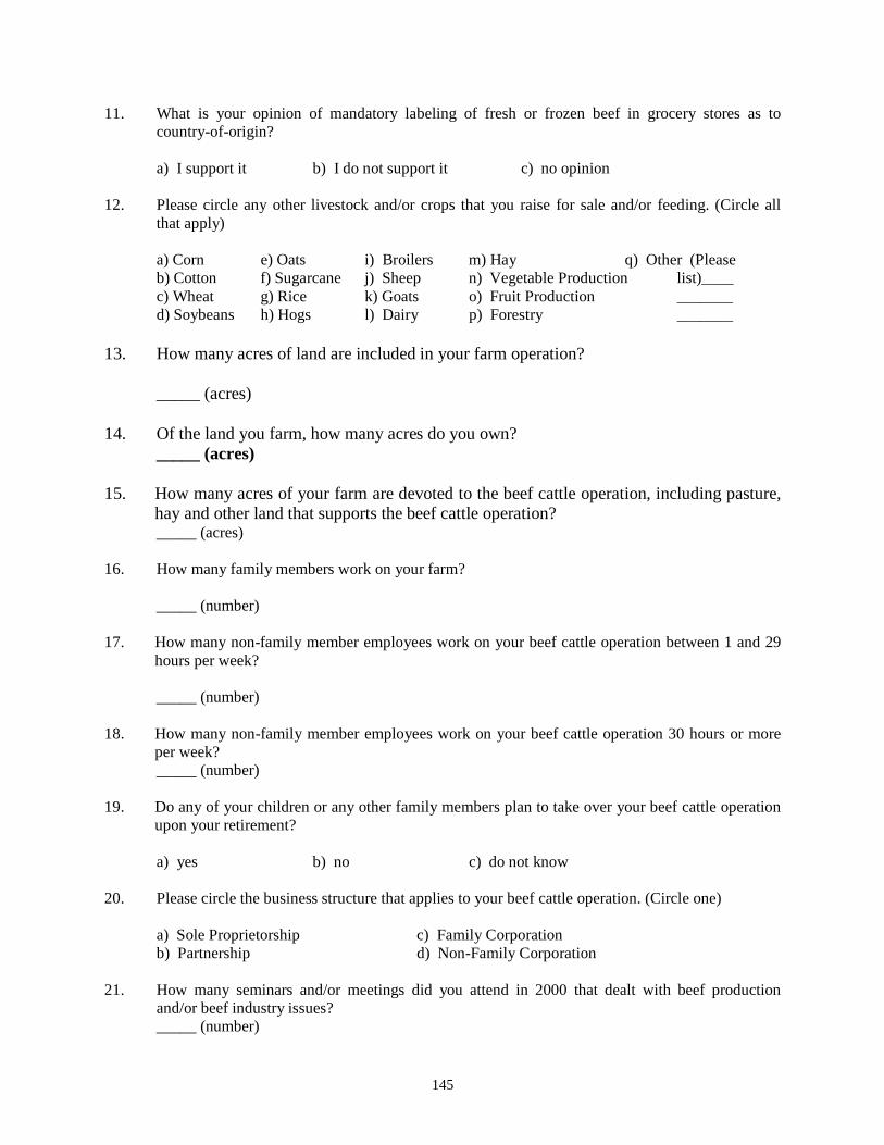
145
11. What is your opinion of mandatory labeling of fresh or frozen beef in grocery stores as to country-of-origin?
a) I support it b) I do not support it c) no opinion
12. Please circle any other livestock and/or crops that you raise for sale and/or feeding. (Circle all
that apply)
a) Corn e) Oats i) Broilers m) Hay q) Other (Please b) Cotton f) Sugarcane j) Sheep n) Vegetable Production list)____ c) Wheat g) Rice k) Goats o) Fruit Production _______ d) Soybeans h) Hogs l) Dairy p) Forestry _______
13. How many acres of land are included in your farm operation?
_____ (acres)
14. Of the land you farm, how many acres do you own?
_____ (acres) 15. How many acres of your farm are devoted to the beef cattle operation, including pasture,
hay and other land that supports the beef cattle operation? _____ (acres)
16. How many family members work on your farm?
_____ (number) 17. How many non-family member employees work on your beef cattle operation between 1 and 29
hours per week? _____ (number)
18. How many non-family member employees work on your beef cattle operation 30 hours or more
per week? _____ (number)
19. Do any of your children or any other family members plan to take over your beef cattle operation
upon your retirement? a) yes b) no c) do not know 20. Please circle the business structure that applies to your beef cattle operation. (Circle one)
a) Sole Proprietorship c) Family Corporation b) Partnership d) Non-Family Corporation
21. How many seminars and/or meetings did you attend in 2000 that dealt with beef production
and/or beef industry issues? _____ (number)

146
22. How many farm magazines did you subscribe to in 2000? (i.e., an annual subscription to Farm Journal would be considered one subscription.)
_____ (number)
23. How many beef-related university publications did you read in 2000?
_____ (number) 24. Are you a member of any beef cattle marketing alliance or cooperative? (Circle one) yes / no
Section II: Goals of Beef Cattle Producers
Beef cattle producers have a number of goals with respect to their operations. Below are some potential goals that you may have for your operation. Please examine each of the following goals and their definitions and then answer the questions that follow. Maintain and Conserve Land: I want to maintain and conserve the land such that it can be preserved for future generations. Maximize Profit: I want to make the most profit each year given my available resources. Increase Farm Size: I want to increase the size of my operation by controlling more land and/or having newer or larger equipment or buildings. Avoid Years of Loss / Low Profit: I want to avoid years of high losses or low profits. I want to avoid being forced out of business. Increase Net Worth: I want to increase my material and investment accumulations. Have Time for Other Activities: I want to have ample time available for activities other than farming, such as leisure or family activities. Have Family Involved in Agriculture: I want my family to have the opportunity to be involved in agriculture.
Some goals are likely to be more important to you than others. Please rank the following set of goals in the order of your perceived importance. Rank the most important goal as “1,” the least important goal as “7,” and each of the others accordingly. Do not use a ranking more than once. In other words, do not rank two or more goals as equal.
Goal Rank
Maintain and Conserve Land: ________
Maximize Profit: ________
Increase Farm Size: ________
Avoid Years of Loss / Low Profit: ________
Increase Net Worth: ________
Have Time for Other Activities: ________
Have Family Involved in Agriculture: ________

147
In this section, you will be asked to compare each of the seven goals with each of the other goals. We are interested in how important each goal is when compared to the other goals. The questions will be worded similar to the one in the following example.
Example: Assume you are asked to compare two goals, maintain and conserve land and increase net worth. If the goal maintain and conserve land is much more important to you than the goal increase net worth, then you would place an “X” very near the goal maintain and conserve land, as shown:
Maintain and conserve land _______________I_______________ Increase net worth On the other hand, if the goal increase net worth is slightly more important to you than the goal maintain and conserve land, then you would place an “X” nearer to the goal Increase net worth, but closer to the middle, as shown:
Maintain and conserve land _______________I_______________ Increase net worth If both goals are equally important, you would place an “X” at the middle of the line.
Maintain and conserve land _______________I_______________ Increase net worth Where the “X” is marked on the line will indicate how much more important one goal is than the other.
As shown above, please indicate your preference for each of the following goals by placing an “X” at the point on the line that best represents your preferences for each comparison. Note that an “X” at the midpoint of a line indicates that both goals are equally important.
Maintain and conserve land _______________I_______________ Maximize profit
Maintain and conserve land _______________I_______________ Increase farm size
Maintain and conserve land _______________I_______________ Avoid years of loss / low profit
Maintain and conserve land _______________I_______________ Increase net worth
Maintain and conserve land _______________I_______________ Have time for other activities
Maintain and conserve land _______________I_______________ Have family involved in ag.
Maximize Profit _______________I_______________ Increase farm size
Maximize Profit _______________I_______________ Avoid years of loss / low profit
Maximize Profit _______________I_______________ Increase net worth
Maximize Profit _______________I_______________ Have time for other activities
Maximize Profit _______________I_______________ Have family involved in ag.
Increase farm size _______________I_______________ Avoid years of loss / low profit
Increase farm size _______________I_______________ Increase net worth
Increase farm size _______________I_______________ Have time for other activities
Increase farm size _______________I_______________ Have family involved in ag.

148
Avoid years of loss/low profit _______________I_______________ Increase net worth
Avoid years of loss/low profit _______________I_______________ Have time for other activities
Avoid years of loss/low profit _______________I_______________ Have family involved in ag.
Increase net worth _______________I_______________ Have time for other activities
Increase net worth _______________I_______________ Have family involved in ag.
Have time for other activities _______________I_______________ Have family involved in ag.
Section III: Risk Attitude and Relationship with Community 1. Relative to other investors, how would you characterize yourself? (Circle one)
a) I tend to take on substantial levels of risk in my investment decisions. b) I neither seek nor avoid risk in my investment decisions. c) I tend to avoid risk when possible in my investment decisions.
2. With respect to your farm operation, how important are each of the following relationships with other members of your community? (Please circle your response)
NI = Not Important at All; NVI = Not Very Important; SI = Somewhat Important; VI = Very Important
a) Relationship with neighboring farmers NI NVI SI VI
b) Relationship with lending institutions (i.e., banks) NI NVI SI VI
c) Relationship with other agricultural businesses NI NVI SI VI
d) Relationship with neighbors who are non-farmers NI NVI SI VI
e) Relationship with other beef cattle producers throughout Louisiana NI NVI SI VI
f) Relationship with regulatory agencies NI NVI SI VI
Section IV: Producer and Farm Characteristics 1. Are you a male or female? (Circle one)
a) male b) female 2. Are you married? (Circle one)
a) yes b) no 3. Which of the following best describes your ethnic background? (Circle one)
a) American Indian c) Black (African American) e) White (Caucasian) b) Asian or Pacific Islander d) Hispanic f) Other____________

149
4. What is your age? ________ (years) 5. What is your level of education? (Circle one)
a) Not a High School Grad. c) Techn. or College Associate’s Deg. e) College Master’s Deg. b) High School Grad. d) College Bachelor’s Deg. f) College Doctoral Deg.
6. How many children 18 years or younger live in your home?
a) None c) 2 e) 4 b) 1 d) 3 f) 5 or more
7. How many years have you been operating your beef cattle farm? ________ (years) 8. How often do you consult with a County agent or other expert in making decisions with respect to
the beef cattle operation? (Circle one)
a) Never b) One to three times per year c) More than three times per year
9. Do you have an off-farm job? (Circle one) yes / no
10. Which of the following best describes your annual household net income? (Circle one)
a) <$20,000 d) $60,000 to $79,999 g) $120,000 to$139,999 b) $20,000 to $39,999 e) $80,000 to 99,999 h) �$140,000 c) $40,000 to $59,999 f) $100,000 to 119,999
11. What percentage of your annual household net income comes from your beef cattle operation?
(Circle one) a) 0 to 20 percent c) 41 to 60 percent e) 81 to 100 percent b) 21 to 40 percent d) 61 to 80 percent 12. What percentage of your annual household net income comes from off-farm employment? (Circle
one) a) Zero c) 21 to 40 percent e) 61 to 80 percent b) 1 to 20 percent d) 41 to 60 percent f) 81 to 100 percent 13. Which of the following best describes your current net worth? (Circle one)
a) <$50,000 c) $100,000 to $199,999 e) $400,000 to $799,999 b) $50,000 to $99,999 d) $200,000 to $399,999 f) �$800,000
14. What is your debt/asset ratio? (Circle one) a) Zero c) 21 to 40 percent e) over 60 percent
b) 1 to 20 percent d) 41 to 60 percent 15. On this farm, which generation does the current operator represent (including your family or your
spouse’s family)? (Circle one)
a) 1st c) 3rd e) 5th b) 2nd d) 4th f) 6th or more
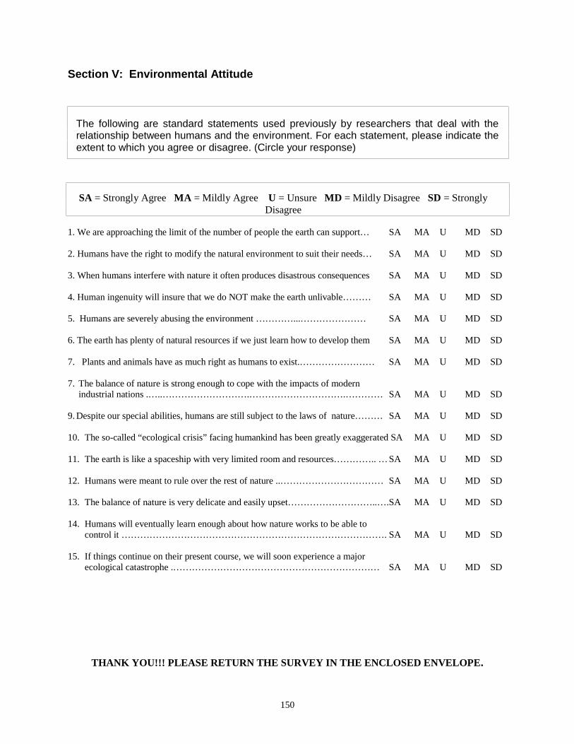
150
Section V: Environmental Attitude
The following are standard statements used previously by researchers that deal with the relationship between humans and the environment. For each statement, please indicate the extent to which you agree or disagree. (Circle your response)
SA = Strongly Agree MA = Mildly Agree U = Unsure MD = Mildly Disagree SD = Strongly Disagree
1. We are approaching the limit of the number of people the earth can support… SA MA U MD SD 2. Humans have the right to modify the natural environment to suit their needs… SA MA U MD SD 3. When humans interfere with nature it often produces disastrous consequences SA MA U MD SD 4. Human ingenuity will insure that we do NOT make the earth unlivable……… SA MA U MD SD 5. Humans are severely abusing the environment …………...………………… SA MA U MD SD 6. The earth has plenty of natural resources if we just learn how to develop them SA MA U MD SD 7. Plants and animals have as much right as humans to exist.…………………… SA MA U MD SD 7. The balance of nature is strong enough to cope with the impacts of modern
industrial nations .…..……………………….………………………….………… SA MA U MD SD 9. Despite our special abilities, humans are still subject to the laws of nature……… SA MA U MD SD 10. The so-called “ecological crisis” facing humankind has been greatly exaggerated SA MA U MD SD 11. The earth is like a spaceship with very limited room and resources………….. … SA MA U MD SD 12. Humans were meant to rule over the rest of nature ..…………………………… SA MA U MD SD 13. The balance of nature is very delicate and easily upset………………………..…. SA MA U MD SD 14. Humans will eventually learn enough about how nature works to be able to control it …………………………………………………………………………. SA MA U MD SD 15. If things continue on their present course, we will soon experience a major ecological catastrophe .………………………………………………………… SA MA U MD SD
THANK YOU!!! PLEASE RETURN THE SURVEY IN THE ENCLOSED ENVELOPE.

151
APPENDIX 2. THE SURVEY QUESTIONNAIRE FOR DAIRY PRODUCERS

152
Use of Conservation Practices and Goals of
Louisiana Dairy Producers ���������

153
Throughout this survey, you will be asked questions about your dairy operation and how you make production decisions. Please check the answer that best reflects your situation. Note that all information is strictly confidential.
Section I: Production Characteristics 1. How many cows in total do you run in your dairy herd?
_____ (number of cows) 2. Do you raise your own replacement heifers? (Circle one)
a) yes b) no 3. What was the average number of pounds of milk produced per cow in your herd in 2000?
_____ lbs/cow 4. Which of the following technologies do you use in your operation? (Circle all that apply) a) Computer b) PC DART program c) Bovine Somatotropin (BSt) d) Artificial Insemination 5. Is your operation a pasture-based operation or a free-stall based operation? (Circle one) a) Pasture-Based Operation b) Free-Stall Based Operation 6. Please circle any other livestock and/or crops that you raise for sale and/or feeding. (Circle all
that apply)
a) Corn e) Oats i) Broilers m) Hay q) Other (Please b) Cotton f) Sugarcane j) Sheep n) Vegetable Production list)____ c) Wheat g) Rice k) Goats o) Fruit Production _______ d) Soybeans h) Hogs l) Beef Cattle p) Forestry _______
7. How many acres of land are included in your farm operation?
_____ (acres) 8. Of the land you farm, how many acres do you own?
_____ (acres) 9. How many acres of your farm are devoted to the dairy operation, including the land
for crops supporting the dairy, hay, silage, pasture, barn, feedlot, etc.
_____ (acres) 10. Do you raise corn for silage on your dairy operation? (Circle one)
a) yes b) no

154
11. How many family members work on your farm? _____ (number) 12. How many non-family member employees work on your dairy operation between 1 and 29 hours
per week? _____ (number)
13. How many non-family member employees work on your dairy operation 30 hours or more per
week? _____ (number)
Section II: Goals of Dairy Producers
Dairy producers have a number of goals with respect to their operations. Below are some potential goals that you may have for your operation. Please examine each of the following goals and their definitions and then answer the questions that follow. Maintain and Conserve Land: I want to maintain and conserve the land such that it can be preserved for future generations. Maximize Profit: I want to make the most profit each year given my available resources. Increase Farm Size: I want to increase the size of my operation by controlling more land and/or having newer or larger equipment or buildings. Avoid Years of Loss / Low Profit: I want to avoid years of high losses or low profits. I want to avoid being forced out of business. Increase Net Worth: I want to increase my material and investment accumulations. Have Time for Other Activities: I want to have ample time available for activities other than farming, such as leisure or family activities. Have Family Involved in Agriculture: I want my family to have the opportunity to be involved in agriculture. Some goals are likely to be more important to you than others. Please rank the following set of goals in the order of your perceived importance. Rank the most important goal as “1”, the least important goal as “7”, and each of the others accordingly. Do not use a ranking more than once. In other words, do not rank two or more goals as equal.
Goal Rank
Maintain and Conserve Land: ________
Maximize Profit: ________
Increase Farm Size: ________
Avoid Years of Loss / Low Profit: ________
Increase Net Worth: ________
Have Time for Other Activities: ________
Have Family Involved in Agriculture: ________

155
In this section, you will be asked to compare each of the seven goals with each of the other goals. We are interested in how important each goal is when compared to the other goals. The questions will be worded similar to the one in the following example:
Example: Assume you are asked to compare two goals, maintain and conserve land and increase net worth. If the goal maintain and conserve land is much more important to you than the goal increase net worth then you would place an “X” very near the goal maintain and conserve land, as shown:
Maintain and conserve land ____________________I____________________ Increase net worth On the other hand, if the goal increase net worth is slightly more important to you than the goal maintain and conserve land then you would place an “X” nearer to the goal Increase net worth, but closer to the middle, as shown:
Maintain and conserve land ____________________I____________________ Increase net worth If both goals are equally important, you would place an “X” at the middle of the line.
Maintain and conserve land ____________________I____________________ Increase net worth Where the “X” is marked on the line will indicate how much more important one goal is than the other.
As shown above, please indicate your preference for each of the following goals by placing an “X” at the point on the line that best represents your preferences for each comparison. Note that an “X” at the midpoint of a line indicates that both goals are equally important.
Maintain and conserve land _______________I_______________ Maximize profit
Maintain and conserve land _______________I_______________ Increase farm size
Maintain and conserve land _______________I_______________ Avoid years of loss / low profit
Maintain and conserve land _______________I_______________ Increase net worth
Maintain and conserve land _______________I_______________ Have time for other activities
Maintain and conserve land _______________I_______________ Have family involved in ag.
Maximize Profit _______________I_______________ Increase farm size
Maximize Profit _______________I_______________ Avoid years of loss / low profit
Maximize Profit _______________I_______________ Increase net worth
Maximize Profit _______________I_______________ Have time for other activities
Maximize Profit _______________I_______________ Have family involved in ag.
Increase farm size _______________I_______________ Avoid years of loss / low profit
Increase farm size _______________I_______________ Increase net worth
Increase farm size _______________I_______________ Have time for other activities
Increase farm size _______________I_______________ Have family involved in ag.

156
Avoid years of loss/low profit _______________I_______________ Increase net worth
Avoid years of loss/low profit _______________I_______________ Have time for other activities
Avoid years of loss/low profit _______________I_______________ Have family involved in ag.
Increase net worth _______________I_______________ Have time for other activities
Increase net worth _______________I_______________ Have family involved in ag.
Have time for other activities _______________I_______________ Have family involved in ag.
Section III: Risk Attitude and Relationship with Community 3. Relative to other investors, how would you characterize yourself? (Circle one)
d) I tend to take on substantial levels of risk in my investment decisions. e) I neither seek nor avoid risk in my investment decisions. f) I tend to avoid risk when possible in my investment decisions.
4. With respect to your farm operation, how important are each of the following relationships with
the other members of your community? (Please circle your response)
NI = not important at all NVI = not very important SI = somewhat important VI = very important
a) Relationship with neighboring farmers NI NVI SI VI
b) Relationship with lending institutions (i.e., banks) NI NVI SI VI
c) Relationship with other agricultural businesses NI NVI SI VI
d) Relationship with neighbors who are non-farmers NI NVI SI VI
g) Relationship with other dairy producers throughout Louisiana NI NVI SI VI
h) Relationship with regulatory agencies NI NVI SI VI Section IV: Producer and Farm Characteristics 1. Are you male or female? (Circle one)
a) male b) female 2. Are you married? (Circle one)
a) yes b) no 3. Which of the following best describes your ethnic background? (Circle one)
a) American Indian c) Black (African American) e) White (Caucasian) b) Asian or Pacific Islander d) Hispanic f) Other____________
4. What is your age? ________ (years)

157
5. What is your level of education? (Circle one)
c) Not a High School Grad. c) Techn. or College Associate’s Deg. e) College Master’s Deg. d) High School Grad. d) College Bachelor’s Deg. f) College Doctoral Deg.
6. How many children 18 years or younger live in your home?
c) None b) 1 c) 2 d) 3 e) 4 f) 5 or more 7. Do any of your children or any other family member plan to take over your dairy operation upon
your retirement? a) yes b) no c) do not know 8. Please circle the business structure that applies to your dairy farm. (Circle one)
a) Sole Proprietorship b) Partnership c) Family Corporation d) Non-Family Corporation
9. Are you a member of a dairy (milk) cooperative? (Circle one) yes / no 10. How many years have you been operating your dairy farm? ________ (years) 11. Do you have an off-farm job? (Circle one)
a) yes b) no 12. Which of the following best describes your annual household net income? (Circle one) a) <$20,000 d) $60,000 to $79,999 g) $120,000 to $139,999 b) $20,000 to $39,999 e) $80,000 to $99,999 h) ≥$140,000 c) $40,000 to $59,999 f) $100,000 to $119,999 13. What percentage of your annual household net income comes from your dairy operation? (Circle
one) a) 0 to 20 percent c) 41 to 60 percent e) 81 to 100 percent b) 21 to 40 percent d) 61 to 80 percent 14. What percentage of your annual household net income comes from off-farm employment? (Circle
one) a) zero c) 21 to 40 percent e) 61 to 80 percent b) 1 to 20 percent d) 41 to 60 percent f) 81 to 100 percent 15. Which of the following best describes your current net worth? (Circle one)
a) <$50,000 c) $100,000 to $199,999 e) $400,000 to 799,999 b) $50,000 to $99,999 d) $200,000 to $399,999 f) ≥$800,000

158
16. What is your debt/asset ratio? (Circle one)
a) zero b) 1 to 20 percent c) 21 to 40 percent d) 41 to 60 percent e) over 60 percent 17. On this farm, which generation does the current operator represent (including your family or your
spouse’s family)? (Circle one)
a) 1st b) 2nd c) 3rd d) 4th e) 5th f) 6th or more 18. In which parish is your dairy farm located? _____________________________(the name of
parish) Section V: Best Management Practices
1. Are you aware of the Coastal Non-Point Pollution Control Program (CNPCP) as specified in the Coastal Zone Management Act? (Circle one) yes / no
2. Are you aware of efforts to control non-point sources of water pollution through the
Clean Water Act? a) yes b) no 3. Have you modified the management of your dairy farm as a result of this legislation? (Circle one)
a) yes b) no c) not applicable 4. How would you rate the quality of surface water in your area? (Circle one)
a) very good b) good c) fair d) poor e) very poor 5. What is your primary source of information about water quality problems? (Circle one)
a) Louisiana Cooperative Extension Service b) Government agencies (Natural Resources Conservation Service (NRCS), and others) c) Farm organizations (Farm Bureau, others) d) Other farmers
6. Have you ever heard about BMPs for dairy operations? (Circle one)
a) yes b) no
If yes, what is your primary source of information? (Circle one)
a) Louisiana Cooperative Extension Service d) Media (Radio, TV, Magazines, etc.) b) Government agencies (NRCS, others) e) Other _________________________
c) Farm organizations (Farm Bureau, others) 7. In your opinion, would/does the use of Best Management Practices on your dairy farm improve
the quality of water leaving your land? (Circle one)
a) yes b) no

159
8. Please check any of the practices that you currently implement under the “yes” column. In cases where you have not implemented a BMP, please indicate your reason for non-implementation under the appropriate “no” column. Please check only one box in each row. A description of the management practices is provided on the following page.
Current Adoption
No
Management Practices
Yes Need More
Information High Cost of Implementation
Have Not Heard of It
Not Applicable to my Farm
Conservation Tillage Practices
Cover and Green Manure Crop
Critical Area Planting
Fence
Field Borders
Filter Strips
Grassed Waterway
Heavy Use Area Protection
Nutrient Management
Pest Management
Prescribed Grazing
Regulating Water in Drainage System
Riparian Forest Buffer
Roof Runoff Management
Sediment Basin
Streambank and Shoreline Protection
Trough or Tank
Waste Management System
Waste Storage Facility
Waste Treatment Lagoon
Waste Utilization

160
Description Conservation Tillage Practices: A system designed to manage the amount, orientation and distribution of crop and other plant residues on the soil surface year-round. Cover and Green Manure Crop: A crop of close growing grasses, legumes or small grains grown primarily for seasonal protection and soil improvement. Critical Area Planting: A planting of vegetation such as trees, shrubs, vines, grasses or legumes on highly erodible areas. Fence: A constructed barrier to livestock, wildlife or people to facilitate the application of conservation practices. Field Borders: Strips of perennial vegetation to control erosion and protect the edges of a field. Filter Strips: Areas of vegetation planted around fields to remove wastewater sediment and nutrients from runoff. Grassed Waterway: A channel that is shaped or graded to required dimensions and established in suitable vegetation to convey runoff from terraces, diversion or other water concentration. Heavy Use Area Protection: Protection of heavily used areas by establishing vegetative cover. Nutrient Management: Management of the amount, form, placement and timing of application of plant nutrients (fertilizers) for optimum forage and crop yields. Pest Management: A pest management program consistent with crop production goals and environmental standards. Prescribed Grazing: Controlled harvest of vegetation with grazing animals. Regulating Water in Drainage System: To control the removal of surface runoff, primarily through the operation of water control structures. Riparian Forest Buffer: An area of trees, shrubs and other vegetation located adjacent to watercourses or water bodies. Roof Runoff Management: A facility for collecting, controlling and disposing of roof runoff water. Sediment Basin: A basin to collect and store debris or sediment. Streambank and Shoreline Protection: Use of vegetation or structures to stabilize and protect banks of streams and lakes against scour and erosion. Trough or Tank: A trough or tank with needed devices for water control and waste disposal installed to provide drinking water for livestock. Waste Management System: A planned system for managing liquid and solid waste including runoff from concentrated waste areas. Waste Storage Facility: An impoundment to temporarily store manure, wastewater and contaminated runoff. Waste Treatment Lagoon: An impoundment to biologically treat organic waste, reduce pollution and protect the environment. Waste Utilization: Use of agricultural waste on land in an environmentally acceptable manner to provide fertility for crop forage, and to improve or maintain soil structure.

161
9. Have you developed and/or updated a dairy farm plan with NRCS within the last three years?
a) yes b) no 10. Of the land on your dairy farm, approximately what percentage would be classified as “highly
erodible”? (Circle one)
a) 0 to 19 percent c) 40 to 59 percent e) 80 to 100 percent b) 20 to 39 percent d) 60 to 70 percent
11. Of the land on your dairy farm, approximately what percentage would you classify as “well-
drained”? (Circle one) a) 0 to 19 percent c) 40 to 59 percent e) 80 to 100 percent b) 20 to 39 percent d) 60 to 70 percent
12. How far from your dairy farm is the nearest neighboring dairy farm? (Circle one)
a) < 1 mile b) 1 to 5 miles c) > 5 miles 13. How far from your dairy farm is the nearest stream or river? (Circle one)
a) a stream / river runs through my farm c) between one-half mile and one mile b) less than half a mile d) more than one mile
14. During the last year, how often did you meet with Louisiana Cooperative Extension Service
personnel? _____ (number of times)
15. During the last year, how often did you meet with NRCS personnel?
_____ (number of times) 16. Are you a member of the Dairy Herd Improvement Association (DHIA)? (Circle one)
a) yes b) no
17. Have you participated in any dairy cost-sharing programs while implementing a BMP? (Circle one) a) yes b) no
18. How many seminars and/or meetings did you attend in 2000 that dealt with dairy production
and/or dairy industry issues? _____ (number) 19. How many farm magazines did you subscribe to in 2000? (i.e., an annual subscription to Farm
Journal would be considered one subscription.) _____ (number)
20. How many dairy-related university publications did you read in 2000? ________ (number)

162
Section V: Environmental Attitude
The following are standard statements used previously by researchers that deal with the relationship between humans and the environment. For each statement, please indicate the extent to which you agree or disagree. (Circle your response)
SA = Strongly Agree MA = Mildly Agree U = Unsure MD = Mildly Disagree SD = Strongly Disagree
1. We are approaching the limit of the number of people the earth can support… SA MA U MD SD 2. Humans have the right to modify the natural environment to suit their needs… SA MA U MD SD 3. When humans interfere with nature it often produces disastrous consequences SA MA U MD SD 4. Human ingenuity will insure that we do NOT make the earth unlivable……… SA MA U MD SD 5. Humans are severely abusing the environment …………...………………… SA MA U MD SD 6. The earth has plenty of natural resources if we just learn how to develop them SA MA U MD SD 7. Plants and animals have as much right as humans to exist.…………………… SA MA U MD SD 8. The balance of nature is strong enough to cope with the impacts of modern
industrial nations .…..……………………….………………………….………… SA MA U MD SD 9. Despite our special abilities, humans are still subject to the laws of nature………SA MA U MD SD 10. The so-called “ecological crisis” facing humankind has been greatly exaggerated SA MA U MD SD 11. The earth is like a spaceship with very limited room and resources………….. … SA MA U MD SD 12. Humans were meant to rule over the rest of nature ..…………………………… SA MA U MD SD 13. The balance of nature is very delicate and easily upset………………………..…. SA MA U MD SD 14. Humans will eventually learn enough about how nature works to be able to control it …………………………………………………………………………. SA MA U MD SD 15. If things continue on their present course, we will soon experience a major ecological catastrophe .………………………………………………………… SA MA U MD SD
THANK YOU!!! PLEASE RETURN THE SURVEY IN THE ENCLOSED ENVELOPE.

163
APPENDIX 3. LETTER INCLUDED IN THE FIRST MAIL OUT FOR BEEF CATTLE PRODUCERS
July 1, 2001 Dear Beef Cattle Producer: The enclosed survey is being sent to you to secure information for use in two studies in the Department of Agricultural Economics and Agribusiness at LSU. The first study provides supporting information for our annual costs and returns estimates for beef cattle production in Louisiana. These estimates are used by producers, lenders, and agribusiness firms throughout Louisiana. This survey will provide farm size, efficiency, and input information for use in developing these estimates. The second study deals with the importance of seven potential goals with respect to beef cattle production. You will note that there are a number of questions on the survey involving producers’ attitudes toward factors such as risk, the environment, and relationships with others in the community. These questions will help us understand how producers make decisions with regard to their cattle operations. This study is being conducted with a graduate student in Agricultural Economics at LSU, and will contribute to his dissertation research. Thus, by filling out the survey, you will be helping him to complete the requirements for his degree. Your participation is very important in assuring that as many producers as possible are represented in this study. The reliability of the survey results depends on the participation of producers such as you. All individual responses will be kept strictly confidential. The questionnaire has an identification number for mailing purposes only. This is so that we may check your name off the mailing list when the questionnaire is returned. Your name will never be placed on the questionnaire. We request that the person with primary decision-making authority on the farm complete the survey. I would be most happy to answer any questions you might have. Please write or call. The telephone number is (225) 578-2759 and my e-mail address is [email protected]. Thank you for your participation. Sincerely, Jeffrey M. Gillespie, Ph.D. Associate Professor

164
APPENDIX 4. LETTER INCLUDED IN THE FIRST MAIL OUT FOR DAIRY PRODUCERS
July 1, 2001 Dear Dairy Producer : As you are aware, many Americans have become concerned in recent years with the impact of agriculture on water quality. This has resulted in increased pressure for farmers to adopt management practices that are �environmentally friendly,� practices that are intended to reduce soil and nutrient runoff into streams. What remains unknown is the extent to which farmers have voluntarily adopted these practices. This survey seeks to determine the extent of adoption of best management practices in the dairy industry, as well as the importance of alternative goals to dairy producers. Your participation in the survey is very important in assuring that as many producers as possible are represented in this study. The reliability of the survey results depends on the participation of producers such as you. All individual responses will be kept strictly confidential. The questionnaire has an identification number for mailing purposes only. This is so that we may check your name off the mailing list when the questionnaire is returned. Your name will never be placed on the questionnaire. We request that the person with primary decision-making authority on the farm complete the survey. Upon receipt of your completed survey, we will send you a check for $10.00. In order for you to receive the payment, you must complete and return the enclosed slip along with the completed survey. The summarized results of the survey will be made available to all interested citizens. Two LSU graduate students in Agricultural Economics will be assisting me in analyzing the data, and will be writing their dissertations based upon the results. Thus, your participation in the study will help them complete their degree requirements. I would be most happy to answer any questions you might have. Please write or call. The telephone number is (225) 578-2759 and my e-mail address is [email protected]. Thank you for your participation. Sincerely, Jeffrey M. Gillespie, Ph.D. Associate Professor

165
APPENDIX 5. POSTCARD FOR BEEF CATTLE PRODUCERS
July 11, 2001 Dear Beef Cattle Producer: Last week, a questionnaire seeking information about your beef cattle operation was mailed to you. The survey deals with beef cattle production efficiency and the importance of alternative goals in beef cattle production. If you have already completed and returned the survey, please accept our sincere thanks. If not, we would appreciate your returning it as soon as possible. It is important that your response be included in the study if the results are to accurately represent the production characteristics of Louisiana beef cattle producers. If by some chance you did not receive the questionnaire, or it was misplaced, please call (225) 578-2759. We will send you another one today. Thank you! Sincerely, Jeffrey M. Gillespie, Ph.D. Associate Professor

166
APPENDIX 6. POSTCARD FOR DAIRY PRODUCERS July 5, 2001 Dear Dairy Producer: Last week, a questionnaire seeking information about your dairy operation was mailed to you. The survey deals with the adoption of best management practices, dairy herd efficiency, and the importance of alternative goals. If you have already completed and returned the survey, please accept our sincere thanks. If not, we would appreciate your returning it as soon as possible. It is important that your response be included in the study if the results are to accurately represent the production characteristics of Louisiana dairy producers. If by some chance you did not receive the questionnaire, or it was misplaced, please call (225) 578-2759. We will send you another one today. Thank you! Sincerely, Jeffrey M. Gillespie, Ph.D. Associate Professor

167
APPENDIX 7. LETTER IINCLUDED IN THE SECOND MAIL OUT FOR BEEF CATTLE PRODUCERS
July 26, 2001 Dear Beef Cattle Producer: About three weeks ago, I wrote to you asking for your participation in a survey about Louisiana cattle producer goals and production practices. As of today, we have not yet received your completed questionnaire. I am writing to you again because of the importance of each survey to the usefulness of this study. The reliability of the study results depends on the participation of producers such as you. The information gathered in this survey will be used in two important studies. The first study will provide supporting information for our annual costs and returns estimates for beef cattle production in Louisiana. These estimates are used by producers and agribusiness firms throughout Louisiana. The survey will provide farm size, efficiency, and input information for use in developing these estimates. The second study deals with the importance of seven alternative goals of cattle producers with respect to their operations. These questions will help us understand how producers make decisions with regard to their cattle operations. This study is being conducted along with a graduate student in Agricultural Economics at LSU, and will contribute to his dissertation research. Thus, by filling out the survey, you will be helping him to complete the requirements for his degree. All individual responses will be kept strictly confidential. No data on individual responses will ever be reported. The questionnaire has an identification number for mailing purposes only. This is so that we may check your name off the mailing list when the questionnaire is returned. Your name will never be placed on the questionnaire. The questionnaire should be completed by the person with primary decision-making authority on the farm. In the event that your survey has been misplaced, a replacement is enclosed. If you have already responded to the survey and we haven’t yet received your response, please accept our sincerest thanks. I would be most happy to answer any questions you might have. Please write or call. The telephone number is (225) 578-2759 and my e-mail address is [email protected]. Your cooperation is greatly appreciated. Sincerely, Jeffrey M. Gillespie, Ph.D. Associate Professor

168
APPENDIX 8. LETTER INCLUDED IN THE SECOND MAIL OUT FOR DAIRY PRODUCERS
July 20, 2001 Dear Dairy Producer : About three weeks ago, I wrote to you asking for your participation in a survey on the use of conservation practices and goals of Louisiana dairy producers. As of today, we have not yet received your completed questionnaire. I am writing to you again because of the importance of each survey to the usefulness of this study. The reliability of the study results depends on the participation of producers such as you. The information gathered in this survey will be used to assess the extent of adoption of best management practices in the dairy industry. Results will allow us to determine which practices are being used and the economic forces that affect adoption. We are also assessing the importance of each of seven producer goals with respect to dairy production. Lastly, information collected in this survey will be help us in estimating our annual costs and returns for dairy production. These estimates are useful management tools for dairy producers throughout Louisiana. The survey results will be analyzed by two graduate students in Agricultural Economics. These students’ dissertations depend upon a good response rate to this study. All individual responses will be kept strictly confidential. No data on individual responses will ever be reported. The questionnaire has an identification number for mailing purposes only. This is so that we may check your name off the mailing list when the questionnaire is returned. Your name will never be placed on the questionnaire. The questionnaire should be completed by the person with primary decision-making authority on the farm. Because of the importance of this study, we will send you a check for $10.00 upon receipt of the survey. To receive the payment, you must complete and return the enclosed slip along with the completed survey. In the event that your survey has been misplaced, a replacement is enclosed. If you have already responded to the survey and we haven’t yet received your response, please accept our sincerest thanks. I would be most happy to answer any questions you might have. Please write or call. The telephone number is (225) 578-2759 and my e-mail address is [email protected]. Your cooperation is greatly appreciated. Sincerely, Jeffrey M. Gillespie, Ph.D. Associate Professor

169
VITA
Aydin Basarir was born in Bismil / Diyarbakir, Turkey, on May 18, 1969. He graduated
from Bismil High School in 1987. He received his Bachelor of Science degree in Agricultural
Economics from Ankara University in 1991. In 1993, while pursuing his Master of Science
degree at Ankara University, he passed a nationwide exam, became a Research Assistant at Gazi
Osman Pasa University and was granted a scholarship to pursue an English training program and
graduate studies in the United States. In 1997, he received his Master of Science degree in
Agricultural Economics from the University of Delaware.
In January 1997, he enrolled in the doctoral program at Louisiana State University in the
Department of Agricultural Economics and Agribusiness. He is now a candidate for the degree
of Doctor of Philosophy, which he will receive in August, 2002.