MULTI-FUNCTION LIDAR SENSORS FOR NON-CONTACT …

MULTI-FUNCTION LIDAR SENSORS FOR NON-CONTACT SPEED AND

TRACK GEOMETRY MEASUREMENT IN RAIL VEHICLES

Shannon A. Wrobel

Thesis submitted to the faculty of the Virginia Polytechnic Institute and State University

in partial fulfillment of the requirements for the degree of

Master of Science

In

Mechanical Engineering

Mehdi Ahmadian, Chair

Corina Sandu

Pablo A. Tarazaga

May 2, 2013

Blacksburg, VA

Keywords: LIDAR, Train Speed, Track Geometry, Track Curvature, Train Distance

MULTI-FUNCTION LIDAR SENSORS FOR NON-CONTACT SPEED AND

TRACK GEOMETRY MEASUREMENT IN RAIL VEHICLES

Shannon A. Wrobel

ABSTRACT

A Doppler LIght Detection And Ranging (LIDAR or lidar) system is studied for the

application of measuring train ground speed in a non-contacting manner, as an alternative

to the current train speed measurement devices such as wheel-mounted tachometers or

encoders. The ability to accurately measure train speed and distance is a critical part of

monitoring track geometry conditions.

Wheel-mounted tachometer speed measurements often fluctuate due to wheel vibrations,

change in wheel diameter, or wheel slip affecting the measurement accuracy. Frequent

calibrations are needed to account for changes in wheel diameter due to wear.

Additionally, the high levels of vibrations at the wheel can cause occasional mechanical

failure of the encoder.

This thesis examines LIDAR as a non-contact train speed measurement device as a direct

retrofit for wheel-mounted encoders. LIDAR uses Doppler technology to accurately

measure train speed. The LIDAR system consists of two laser sensors and can be

installed on either the car body or the truck on the underside of the train. The sensors

measure the true ground speed of each rail, from which the track curvature can then be

assessed based on the difference between the right and left rail speeds. The LIDAR train

speed, distance, and curvature results are then evaluated against encoder readings and

other conventional train measurement devices.

Various tests were performed, including field-testing onboard a track geometry railcar

operated by Norfolk Southern for evaluating the efficacy, accuracy, and durability of the

LIDAR system; and laboratory tests on a 40-foot rail panel for assessing the ability to

obtain measurements at super low speeds.

iii

The test results indicate that when compared with other conventional means used by the

railroad industry, LIDAR is capable of accurately measuring train speed and distance

from speeds as slow as 0.3 mph and up to 100 mph. Additionally, the curvature

measurements proved to be as accurate as Inertial Measurement Units (IMUs) that are

commonly used in track geometry measurement railcars.

iv

Dedication

I would like to dedicate this thesis to my amazing family, friends, and boyfriend who

have made all of this possible and been there to support me every step of the way. I am

eternally grateful.

v

Acknowledgements

First of all, I greatly acknowledge and appreciate the financial support provided by the

Federal Railroad Administration Office of Research and Development under the direction

of Mr. Cameron (Cam) Stuart. The continuous support of Masseurs Cam Stuart and Gary

Carr (also of FRA) was critical in the success of this program.

I would like to thank my research advisor, Dr. Mehdi Ahmadian, the lab supervisor,

Michael Craft, and fellow graduate research assistant, Josh Munoz, for their support,

guidance, and assistance throughout my graduate research.

I am also indebted to the Norfolk Southern Research and Tests Department for their

tremendous technical support and many invaluable discussions. Most of the tests and

findings discussed in this report could not have been completed without the help of many

of the Norfolk Southern employees including Barry Radford, Brad Kerchof, James

Harris, Lee Turner, Mike Hedrick, Noah Robison, Scott Hailey, Sean Woody, Steve

Smith, and Tim Childress.

The system support provided by Mr. Carvel Holton (independent consultant) and Mr.

Mark Beaubien of Yankee Environmental Systems (YES) is also greatly

appreciated. The efforts of all of our partners at FRA, NS, and YES were instrumental in

achieving the goals of this program. All views expressed in this publication are those of

the author’s and do not necessarily reflect the views of the sponsors and technical

partners.

vi

Contents

Dedication .......................................................................................................................... iv

Acknowledgements ............................................................................................................. v

Contents ............................................................................................................................. vi

List of Figures .................................................................................................................. viii

List of Tables ...................................................................................................................... x

List of Abbreviations ......................................................................................................... xi

1 Introduction ................................................................................................................. 1

1.1 Thesis Overview ................................................................................................... 1

1.2 Objective .............................................................................................................. 1

1.3 Approach .............................................................................................................. 2

1.4 Outline .................................................................................................................. 2

1.5 Contributions ........................................................................................................ 3

2 Background ................................................................................................................. 4

2.1 LIDAR .................................................................................................................. 4

2.1.1 Doppler LIDAR Technology ........................................................................ 4

2.1.2 LIDAR Technology Benefits ........................................................................ 7

2.2 Speed Measurement in the Rail Industry ............................................................. 8

2.3 Curvature Measurement in the Rail Industry ..................................................... 10

2.4 Literature Study .................................................................................................. 11

2.4.1 Approach ..................................................................................................... 11

2.4.2 LIDAR ........................................................................................................ 11

2.4.3 Train Speed Measurements ......................................................................... 14

2.4.4 Track Curvature Measurements .................................................................. 19

3 Field Testing ............................................................................................................. 25

3.1 System Description ............................................................................................ 25

3.2 System Track Geometry Car Installation ........................................................... 26

3.3 Field Testing ....................................................................................................... 28

3.3.1 Truck-Mounted LIDAR System Testing .................................................... 28

3.3.2 Car-Mounted LIDAR System Testing ........................................................ 31

3.3.3 Laboratory LIDAR Testing......................................................................... 32

3.4 Field Test Data Processing ................................................................................. 34

vii

4 System Test Results .................................................................................................. 38

4.1 Truck-Mounted LIDAR System Measurements ................................................ 38

4.1.1 Speed Measurements .................................................................................. 38

4.1.2 Distance Measurements .............................................................................. 41

4.1.3 Curvature Measurements ............................................................................ 42

4.2 Body-Mounted LIDAR System Measurements ................................................. 46

4.2.1 Speed Measurements .................................................................................. 46


4.2.3 Curvature Measurements ............................................................................ 50

4.2.4 Alignment Measurements ........................................................................... 51

4.3 Laboratory LIDAR Measurements..................................................................... 53

4.3.1 Speed Results .............................................................................................. 54


5 Summary and Conclusion ......................................................................................... 58

5.1 Summary ............................................................................................................ 58

5.2 Conclusions ........................................................................................................ 59

5.3 Recommendations for Future Studies ................................................................ 60

References ......................................................................................................................... 61

viii

ListofFigures

Figure 1: LIDAR concept for measuring speed in a non-contacting manner for railroad

applications ......................................................................................................................... 4

Figure 2: System-level block diagram of multifunction LIDAR sensors for non-contact

speed and complex rail dynamics measurements ............................................................... 6

Figure 3: An encoder/tachometer attached to train wheel .................................................. 9

Figure 4: Yaw, pitch, and roll of a plane in a similar fashion to a train [4] ...................... 10

Figure 5: The IMU installed on the bogie in front of the encoder (axle generator) and the

placement of other test equipment on a track geometry car ............................................. 11

Figure 6: The LIDAR mounting for helicopter speed testing [17] ................................... 13

Figure 7: Differential Global Positioning System to detect train location [6] .................. 16

Figure 8: Two eddy current sensors to determine train speed [34] ................................... 18

Figure 9: The concept of a mid-chord offset measurement [39] ...................................... 20

Figure 10: Curvature measurements using a 62-foot-length chord [42] ........................... 21

Figure 11: The LIDAR mounting setup on the track geometry car .................................. 26

Figure 12: The PXI (left) and KVM (right) equipment utilized in parallel with the LIDAR

sensors ............................................................................................................................... 26

Figure 13: TOR, gauge face, and web beam alignments were tested to select the best

performing configuration .................................................................................................. 27

Figure 14: A side view of the TOR, gauge corner, and web of rail beam configurations

showing the optic fiber connections to the lenses ............................................................. 28

Figure 15: The truck-mounted LIDAR system with the lenses facing the Top of Rail .... 29

Figure 16: Explosion-proof protective housing securing the LIDAR lenses onboard the

track geometry car............................................................................................................. 30

Figure 17: The dirt build-up over the entire truck-mounted test train trip ........................ 30

Figure 18: The car-mounted LIDAR setup with the lenses facing the gauge corner ....... 31

Figure 19: The modified lens housings with the connected positive air flow supply ....... 32

Figure 20: LIDAR sensors setup on ‘track trolley’ for short rail testing .......................... 33

Figure 21: Encoder setup on the ‘track trolley’ ................................................................ 34

Figure 22: A flow chart of the code processes .................................................................. 37

Figure 23: A comparison of the LIDAR, encoder, and GPS speed results from Roanoke,

VA to Elliston, VA ........................................................................................................... 39

Figure 24: LIDAR vs. encoder speed from Roanoke, VA to Elliston, VA ...................... 40

Figure 25: A close-up of the LIDAR vs. encoder speed measurements ........................... 40

Figure 26: LIDAR vs. encoder distance from Roanoke, VA to Elliston, VA .................. 41

Figure 27: A close-up comparison of the LIDAR vs. encoder distance measurements ... 42

Figure 28: A comparison of the IMU and LIDAR curvature readings from Roanoke, VA

to Elliston, VA .................................................................................................................. 43

Figure 29: The IMU and LIDAR curvature from Roanoke, VA to Elliston, VA over 1.5

mile stretch ........................................................................................................................ 44

Figure 30: The chordal, FRA, Highrail, IMU, and LIDAR curvature measurements near

Elliston, VA ...................................................................................................................... 45

ix

Figure 31: A comparison of LIDAR curvature results as the train travels east- and

westbound ......................................................................................................................... 46

Figure 32: A comparison of the LIDAR and encoder data provided by NS from Roanoke,

VA to Christiansburg, VA ................................................................................................ 47

Figure 33: The LIDAR and encoder speed over a one-mile stretch in Glenvar, VA ....... 48

Figure 34: A comparison of the LIDAR and encoder distance measurements vs. time for

about 165 miles ................................................................................................................. 49

Figure 35: A close-up of the LIDAR and encoder distance measurements over time ..... 49

Figure 36: A comparison of LIDAR and IMU curvature measurements from Roanoke,

VA to Christiansburg, VA ................................................................................................ 51

Figure 37: LIDAR vs. IMU curvature measurements for approximately 1.5 miles of

railway track...................................................................................................................... 51

Figure 38: A comparison of the LIDAR vs. IMU alignment readings over about 1.5 miles

of track .............................................................................................................................. 52

Figure 39: A comparison of the LIDAR vs. IMU alignment readings near Wysor, VA .. 53

Figure 40: The PXI computer with product filter attachments ......................................... 54

Figure 41: A comparison of the left and right rail LIDAR speed results vs. the encoder

speed over 6ft .................................................................................................................... 55

Figure 42: A comparison of the left and right rail LIDAR speed results vs. the encoder

speed over 12ft .................................................................................................................. 55

Figure 43: Encoder vs. LIDAR distance measurements over time ................................... 56

Figure 44: A close-up of the Encoder vs. LIDAR distance measurements over time ...... 57

x

ListofTables

Table 1: The mid-chord offset calculations and table of values [43] ............................... 21

xi

ListofAbbreviations

ATGMS

CARAT

CAS

Autonomous Track Geometry Measurement

Systems

Computer and Radio Aided Train

Collision Avoidance System

CPU Central Processing Unit

CVeSS

DGPS

DIAL

Center for Vehicle Systems and Safety

Differential GPS

Differential Absorption LIDAR

FFT

FOG

Fast Fourier Transform

Fiber Optic Gyro

FRA

FWHM

Federal Railway Administration

Full Width Half Maximum

GPS Global Positioning System

IMU Inertial Measurement Unit

KVM Keyboard, Video, and Mouse

LIDAR

MEMS

MSIMS

Light Detection and Ranging

MicroElectroMechanical Systems

Multiple Sensor Inertial Measurement System

MTTF

NI

Mean Time to Failure

National Instruments

NS Norfolk Southern

PTC

RADAR

RLG

RTL

SPS

SWG

TG

Positive Train Control

Radio Detection and Ranging

Ring Laser Gyro

Railway Technologies Laboratory

Standard Positioning Service

Spinning Wheel Gyro

Track Geometry

TOR Top of Rail

VT

YES

Virginia Tech

Yankee Environmental Systems

1

1 Introduction

1.1 Thesis Overview

LIDAR, or Light Detection and Ranging, is a non-contact speed measurement system.

LIDAR utilizes the Doppler Effect, in which the LIDAR sensor emits laser light onto the

rail at a set frequency, which is then reflected back to the sensor with a phase shift based

on the relative speed of the track. The Doppler shift received by the sensor is used to

accurately determine the train’s speed [1]. Other track speed measurement systems in use

by the U.S. railroads today include encoders, GPS, Radar, and ground truth measurement

systems, often generate speed measurement errors due to slip, wear, train vibration, or

mechanical issues encountered throughout train trips. As a non-contact measurement

system, the LIDAR sensors eliminate these issues. Moreover, the LIDAR system is able

to accurately measure speed over a wider range than the other systems, from speeds as

low as 0.3 mph to those as large as 100 mph. In addition to speed measurements, the

LIDAR sensors can accurately determine distance and track curvature through post-

processing. Speed, distance, and track geometry measurements are a critical part of track

analysis for track safety. Thus, LIDAR’s reliability and versatility could make it a

practical and superior alternative to current track measurement and testing technologies.

1.2 Objective

The primary objectives of this study are to:

1. Demonstrate the applicability of LIDAR to determine train speed, distance, and

track curvature for railway applications.

2. Prove LIDAR’s ability to measure speed, track curvature, and distance accurately.

3. Determine the preferred installation setup and lens configuration for the LIDAR

system on the track geometry car through rigorous railway conditions.

2

4. Establish if LIDAR is capable of replacing wheel-mounted encoders and Inertial

Measurement Units (IMUs) currently used to measure train speed, distance, and

track curvature on track geometry cars.

5. Describe the potential advantages and disadvantages of the LIDAR system and

discuss future goals to develop LIDAR as a market worthy, non-contacting,

multifunctional sensor system.

1.3 Approach

In order to determine the capabilities, applicability, and accuracy of LIDAR for railway

applications, the following steps were taken:

1. Upon completion of preliminary LIDAR lab and track tests, the LIDAR system

was mounted to the underside of the track geometry car to test the LIDAR system

out in the field. The LIDAR system was mounted either to the truck or the car

body of the track geometry car to assess the accuracy and durability of the system

over a significant number of miles at high speeds and under railway conditions.

2. Additionally, slow speed LIDAR testing was completed at the Railway

Technologies Lab by using a ‘track trolley’ on a short piece of track with the

lenses facing gauge corner. This allowed the LIDAR system to be assessed for

reliability and accuracy in measuring speed and distance at low speeds.

3. The data procured over these tests was analyzed through post-processing to

determine the train speed, distance, and track curvature. The LIDAR results are

then benchmarked against encoder and Inertial Measurement Unit (IMU) data.

1.4 Outline

Chapter 2 provides an in-depth overview of Doppler LIDAR and its applicability in

railroad applications. The current methods of train speed and curvature detection are then

discussed. Lastly, a thorough literature study of the different applications of LIDAR and

the various techniques to measure train speed and curvature used throughout the years is

presented.

3

Chapter 3 describes the LIDAR tests setups on the track geometry car and in the Railway

Technologies Lab (RTL), as well as the post-processing computations and code.

In Chapter 4, the results of the field tests depicted in Chapter 3 are compared to the

conventional railroad measurements.

Chapter 5 illustrates the major findings, conclusions, and recommendations for future

work.

1.5 Contributions

The main contributions of this study are:

1. Development of an advanced and accurate system to measure train speed,

distance, and curvature with the LIDAR sensors.

2. Demonstration of the viability of LIDAR as a commercially viable product, with

further developments for multipurpose use in the railway industry for low and

high speeds.

3. Illustration of LIDAR’s potential to measure track alignment and other track

geometry measurements with further testing.

4

2 Background

2.1 LIDAR

2.1.1 Doppler LIDAR Technology

LIDAR directly measures speed in a non-contacting manner by use of the Doppler Effect.

The Doppler LIDAR sensors operate by emitting a single laser pulse at a specific

wavelength towards the object of interest; the laser is then reflected back to the receiver

at a different wavelength, creating a Doppler Shift. The combination of the travel time of

the laser pulse and the Doppler shift allow for the speed of the object to be determined

[1]; in this case, a moving railcar relative to the track. Incidentally, this is the same

technology that law enforcement uses to catch speeding drivers.

Figure 1 displays the concept of using LIDAR sensors for determining rail speed. The

Doppler LIDAR sensors can be attached to the underside of a track geometry car with

two laser beams facing the left and right rails. The dashed arrow indicates the outgoing

LIDAR beam, and the dotted-dashed arrow shows the same beam reflected back to the

sensors, which detect the Doppler shift for each rail.

Figure 1: LIDAR concept for measuring speed in a non-contacting manner for

railroad applications

�

5

The LIDAR Doppler shift data is then passed through a High Fidelity RF device to

produce the left and right rail frequency data. This data is then processed into a National

Instruments (NI) PXI central processing unit (CPU), as shown in Figure 2. The PXI CPU

has been specifically configured for this study to generate a Fast Fourier Transform

(FFT) of the LIDAR signals. The FFT transforms the frequency data to determine the

velocity for the left and right rails in real time. With the velocity from each rail, the PXI

then calculates the track speed, based on the average velocities from both rails.

Additionally, the track curvature can be determined based on the speed difference

between the two rails. The track speed and curvature results are then displayed onto a

monitor and saved to a hard drive. The saved data from the hard drive is post-processed

to establish further capabilities of the LIDAR system beyond speed and curvature. In

particular, the travel distance is ascertained through post-processing, similar to the

distance measured by a conventional encoder. Additionally, during post-processing, the

LIDAR data is assessed for potential detection track alignment results. As a non-contact

measurement system, the LIDAR sensors prove to be reliable and accurate in rail

measurements. The goal is to utilize LIDAR as a direct retrofit for encoders and IMUs

on a track geometry car, allowing the system to run unmanned for several hundreds of

miles.

6

Figure 2: System-level block diagram of multifunction LIDAR sensors for non-

contact speed and complex rail dynamics measurements

7

2.1.2 LIDAR Technology Benefits

The benefits of LIDAR technology, as compared with existing track speed and curvature

measurements, particularly for high speeds and/or elevated safety environments, are:

1. A non-contact measurement technology that eliminates the many speed-dependent

design complexity, reliability, maintenance, and accuracy (slip) issues and

limitations (e.g., vibration) of mechanically contacting or axle-linked tachometers

(analog or digital).

2. A non-contact, Doppler measurement technology with:

a. Inherently high accuracy that is speed-independent, and has an absolute

scale factor (580KHZ/mph) which is not subject to wear, track speed (slip

and data rate), spatial resolution/standoff (Radar), environment, etc.

b. Continuous, consistent operation over a wider range of track speeds (creep

speed to hundreds of mph) that exceeds any current technology

(analog/digital tachometers, radar, GPS, etc.)

c. Consistent track curvature measurement at far slower speeds than possible

with Inertial Measurement Units (IMUs) that are commonly used in track

geometry rail cars

d. Suitability for autonomous operation in generic revenue service or high-

precision track metrology applications, e.g., Autonomous Track Geometry

Measurement Systems (ATGMS)

e. Capability for detecting auxiliary parameters critical to autonomous, in-

motion safety and just-in-time maintenance in High Speed Rail or Intercity

Passenger Service; for example, instantaneous curvature, GPS position

correction (PTC), and possibly rail condition and stability.

3. A non-contact, optical measurement technology that uses the following:

a. Telecommunications wavelengths at 1.5um:

i. Highest, inherent eye safety

8

ii. 10,000 times higher spatial precision and speed accuracy relative

to Radar

iii. Demonstrated performance in rain against wet/iced/snow surfaces

iv. Reduced cost components with increased Mean Time to Failure

(MTTF) and suited to environmental extremes as compared with

typical laser optics.

b. Telecommunications optical fibers:

i. Flexible, arbitrary mounting locations for easier system integration

ii. Fixed, no-maintenance internal optical alignments.

c. Coherent detection, resulting in larger dynamic detection ranges than

conventional intensity-based optical metrology sensors used for rail

applications:

i. Reduced maintenance – tolerant of dirtier lenses and windows,

rain, mist, etc.

ii. Reduced diameter optics (1/4 – 1in) and/or increased non-contact

ranges (millimeters to meters)

iii. Detects scattered light sensing on all surface materials (rock, steel,

ice/snow, etc.), roughness (e.g., shiny or coarse), and colors (e.g.,

light or dark) while rejecting sun or artificial lighting (e.g.,

headlamps, etc.).

2.2 Speed Measurement in the Rail Industry

Railway transportation systems most commonly measure train speed with axle encoders

(also known as tachometers, odometers, or generators). These encoders are attached to

the end of the solid axle wheel of the train, as shown in Figure 3. Encoders record

distance traveled as the train moves along the train tracks by determining the number of

wheel rotations and multiplying this by the circumference of the wheel. Additionally, the

encoders can measure the distance between transponders or beacons in very small

9

increments known as a ‘foot-pulse’. The ‘foot-pulse’ demarcation provides a visual for

any distance error build-up and need for recalibration over time. Based on the distance

results from the encoder, the train speed can also be determined by differentiating the

distance results. However, the encoder often generates errors over time due to slip,

wheel/rail wear, and other factors, which requires frequent recalibration of the encoder.

This error build-up propagates into the distance and speed measurements, creating

inaccuracy and unreliability in encoder measurements.

Currently, there are magnetically-driven and optically-driven tachometers that are both

utilized in the railway industry. Magnetically-driven tachometers generally produce more

errors than optically-driven devices, and are only capable of measuring direction/speed in

one direction. Optically-driven tachometers can record data at very slow speeds, thus

making them more accurate than magnetic units. Additionally, the optically-driven

encoders can measure data when the train is moving forward and backward [2].

There are several other methods that have been adopted by various U.S. railroads to

measure speed; these include GPS, Doppler Radar, Inertial Measurement Units, and

several others. These methods will be discussed in further detail in the Literature Study

section.

Figure 3: An encoder/tachometer attached to train wheel

10

2.3 Curvature Measurement in the Rail Industry

Common practice to determine track curvature in the rail industry consists of utilizing

Inertial Measurement Units (IMUs). Inertial measurement units are comprised of three

accelerometers and three gyroscopes to measure the accelerations experienced by the

train, as well as the pitch, yaw, and roll of the train. Figure 4 presents the orientation of

pitch, yaw, and roll. Upon encountering a curve, the train yaws and experiences

centrifugal forces, which are recorded by the IMU; thus, the degree of curvature of the

track can be calculated accordingly [3].

Figure 4: Yaw, pitch, and roll of a plane in a similar fashion to a train [4]

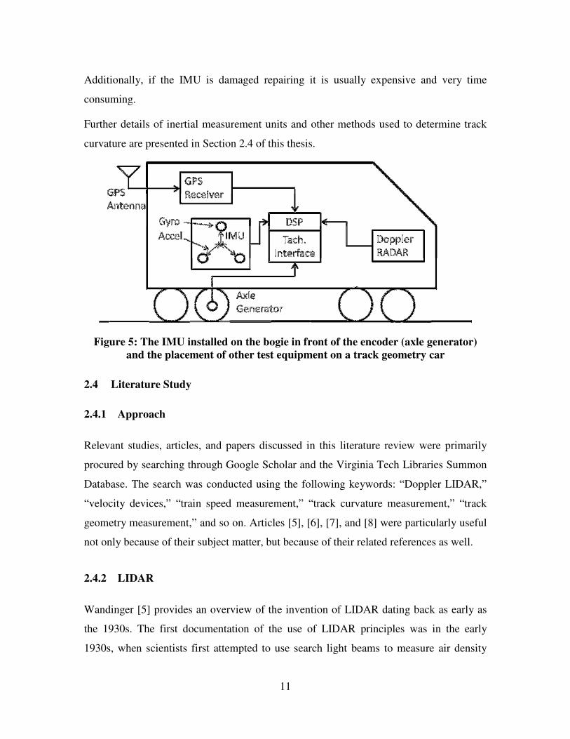
The IMU is attached to the truck of the track geometry car near the wheel axle. The

installation of an IMU relative to an encoder’s placement is presented in Figure 5. This

figure also displays other track geometry car test equipment mounting including Doppler

radar and GPS, which will be discussed further later. The IMU system mounted directly

to the truck proves advantageous as it eliminates any body dynamics experienced by the

train, thus presenting a more accurate representation of the track geometry. However,

IMUs often experience issues in accurately determining curvature at low speeds.

Yaw Axis

Roll Axis

Pitch Axis

11

Additionally, if the IMU is damaged repairing it is usually expensive and very time

consuming.

Further details of inertial measurement units and other methods used to determine track

curvature are presented in Section 2.4 of this thesis.

Figure 5: The IMU installed on the bogie in front of the encoder (axle generator)

and the placement of other test equipment on a track geometry car

2.4 Literature Study

2.4.1 Approach

Relevant studies, articles, and papers discussed in this literature review were primarily

procured by searching through Google Scholar and the Virginia Tech Libraries Summon

Database. The search was conducted using the following keywords: “Doppler LIDAR,”

“velocity devices,” “train speed measurement,” “track curvature measurement,” “track

geometry measurement,” and so on. Articles [5], [6], [7], and [8] were particularly useful

not only because of their subject matter, but because of their related references as well.

2.4.2 LIDAR

Wandinger [5] provides an overview of the invention of LIDAR dating back as early as

the 1930s. The first documentation of the use of LIDAR principles was in the early

1930s, when scientists first attempted to use search light beams to measure air density

12

profiles in the upper atmosphere. Then, in 1938, for the first time cloud height was

measured using light pulses.

The term LIDAR arose in 1953 when Middleton and Spilhuas created a method of using

a light pulse transmitter and a receiver to determine the height of an object [9]. However,

it wasn’t until 1960 when the laser was invented and the modern LIDAR technology

came about. Subsequently, LIDAR lasers rapidly became used in a number of different

fields of research.

There are two main types of LIDAR that are currently used: incoherent (or direct energy)

detection, and coherent detection, which use Doppler or phase shift measurement as

described in [10]. There are three main types of coherent LIDAR systems: Range

Finders, DIAL, and Doppler LIDAR. Range finders are used to measure the distance

from the LIDAR device to a solid target. DIAL (Differential Absorption LIDAR) utilizes

two different LIDAR wavelengths to measure chemical concentrations in the atmosphere.

Doppler LIDARs measure the velocity of a moving object based on the Doppler shift

when the laser is reflected back from the moving object [11]. Of these, the focus of this

literature study will be on Doppler LIDARs.

One application of Doppler LIDAR sensors is to monitor wind speeds for air traffic

safety. Inokuchi et al. [12] discuss the effect of wind turbulence on the number of aircraft

accidents, and determined that detecting the wind turbulence in advance is a crucial part

of aircraft safety. In order to detect wind turbulence, originally Radio Detection and

Ranging, or RADAR, was used onboard aircrafts, but this showed inconsistency in

detecting sudden wind turbulence in areas without clouds or rain. In 2007, the Japan

Aerospace Exploration Agency tested Doppler LIDAR on aircrafts to replace Radar [12]

by emitting a laser pulse, which is reflected off of air particulates in the wind to

determine wind speed. The LIDAR showed promise in detecting wind turbulence

onboard aircrafts and proved to be much more reliable than Radar. Similarly, in 2002, the

Hong Kong International Airport utilized Doppler LIDARs to identify terrain-induced

wind shear, which affects airplane landings and takeoffs. The LIDAR was attached to the

ground traffic control tower of the Hong Kong International Airport to assess

departure/approach airway lanes for wind shears. In this study, the LIDAR provided

13

accurate detection of the wind shear and is still currently used at the Hong Kong

International Airport [13].

Additionally, Doppler LIDAR sensors are used to measure offshore wind speeds for

production of wind turbine energy. Koch et al. [14] and Pichugina et al. [15] discuss the

use of LIDAR onshore and onboard ships, respectively, to determine wind speeds for

turbine energy with reasonably good accuracy.

LIDAR is also capable of measuring wind speed in real time. This is evident in [16],

which describes that in the 2008 Olympics in China, the competitive sailors used LIDAR

as a means of detecting wind speed in real time. This assisted the sailors in determining

the wind speed and the direction of the wind much faster and more accurately than with

buoys.

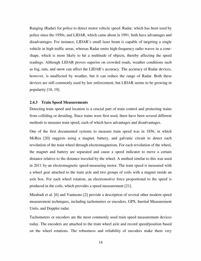
Apart from wind speed detection, LIDAR was also used by the NASA Langley Research

Center to evaluate helicopter speed in 2009 [17]. In this test, NASA mounted the LIDAR

towards the nose of the helicopter in the white spherical housing shown in Figure 6. Six

tests were completed on the helicopter in order to obtain not only the helicopter’s speed,

but its altitude as well. The results for both speed and altitude were compared to GPS

readings and showed excellent correlation for both measurements.

Figure 6: The LIDAR mounting for helicopter speed testing [17]

LIDAR sensors are most widely known for speed detection in vehicles for law

enforcement purposes. LIDAR is currently used as an alternative to Radio Detection and

14

Ranging (Radar) for police to detect motor vehicle speed. Radar, which has been used by

police since the 1950s, and LIDAR, which came about in 1991, both have advantages and

disadvantages. For instance, LIDAR’s small laser beam is capable of targeting a single

vehicle in high traffic areas, whereas Radar emits high-frequency radio waves in a cone-

shape, which is more likely to hit a multitude of objects, thereby affecting the speed

readings. Although LIDAR proves superior on crowded roads, weather conditions such

as fog, rain, and snow can affect the LIDAR’s accuracy. The accuracy of Radar devices,

however, is unaffected by weather, but it can reduce the range of Radar. Both these

devices are still commonly used by law enforcement, but LIDAR seems to be growing in

popularity [18, 19].

2.4.3 Train Speed Measurements

Detecting train speed and location is a crucial part of train control and protecting trains

from colliding or derailing. Since trains were first used, there have been several different

methods to measure train speed, each of which have advantages and disadvantages.

One of the first documented systems to measure train speed was in 1856, in which

McRea [20] suggests using a magnet, battery, and galvanic circuit to detect each

revolution of the train wheel through electromagnetism. For each revolution of the wheel,

the magnet and battery are separated and cause a speed indicator to move a certain

distance relative to the distance traveled by the wheel. A method similar to this was used

in 2011 by an electromagnetic speed-measuring motor. The train speed is measured with

a wheel gear attached to the train axle and two groups of coils with a magnet inside an

axle box. For each wheel rotation, an electromotive force proportional to the speed is

produced in the coils, which provides a speed measurement [21].

Mirabadi et al. [6] and Vantuono [2] provide a description of several other modern speed

measurement techniques, including tachometers or encoders, GPS, Inertial Measurement

Units, and Doppler radar.

Tachometers or encoders are the most commonly used train speed measurement devices

today. The encoders are attached to the train wheel axle and record speed/position based

on the wheel rotations. The robustness and reliability of encoders make them very

15

desirable for train speed measurement [22]. Encoders, however, are often limited by

resolution, sampling time, electrical noise, and slipping and sliding between the wheel

and the track [6]. Due to the fact that the encoder is attached to the wheel, slipping and

sliding alters the distance and speed measurements and generates inaccuracies. Several

studies have worked towards correcting this slide and slip error in the encoder. Saab et al.

[23] suggest using a Kalman filter to observe the speed and acceleration readings. Then if

the velocity readings meet a certain condition, the velocity results are adjusted by using

linear interpolation between the speed before and after the slip/slide error. Ikeda [24]

studied a system called Computer and Radio Aided Train (CARAT) to detect train

distance in order to analyze slip/slide error and eliminate these errors from the results.

Allota et al. [25] recommend utilizing an algorithm that estimates the train’s speed and

position during start/stop accelerations by using two encoders placed on two different

axles.

GPS devices are also used to measure train speed and distance. GPS systems are most

often used to determine train location to prevent collisions and allow for appropriate

spacing between trains. The train location is determined using at least four satellites and

evaluating the travel time between each of the satellites and the GPS receiver (mounted to

the top of the train car) based on the location of the satellites. The speed can then be

calculated directly by using the Doppler principle [6]. GPS devices are beneficial for

determining a train’s location and speed for such applications as the Alaska Railroad’s

Collision Avoidance System (CAS), which allows dispatchers and trains to monitor train

locations and improve safety [26]. GPS systems have several disadvantages, however.

First, the GPS satellite signal available to the public known as Standard Positioning

Service (SPS) is ‘dithered’ by the military, which lowers the accuracy of the readings, in

order to prevent overuse of the system. The best way to increase the accuracy of SPS is to

use a Differential GPS (DGPS) as shown in Figure 7. The DGPS requires a stationary

land-based transponder to reduce the dither error, and generates an accurate measurement

within ±20cm [27]. Without a DGPS, the accuracy of a GPS is about ±5m, which means

that it cannot distinguish between two parallel train tracks. Additionally, a GPS does not

receive a signal underground or in tunnels. This can significantly limit the availability

and accuracy of the GPS signal in certain areas [2].

16

Figure 7: Differential Global Positioning System to detect train location [6]

Another commonly-used method of measuring train speed is an Inertial Measurement

Unit (IMU). IMUs typically consist of both an accelerometer and a gyroscope.

Accelerometers measure the inertial forces experienced by the train, from which the

acceleration can then be derived. The acceleration is then integrated to obtain the speed

and position of the train. In order to accurately determine forward train speed, the

accelerometers should not be sensitive to vertical and lateral accelerations. Also, the

accelerometer sensor must be perfectly horizontal to avoid detecting accelerations due to

gravity [22]. Gyroscopes measure angular rotation of the train. Currently, Spinning

Wheel Gyros (SWG), Ring Laser Gyros (RLG), and Fiber Optic Gyros (FOG) are the

most common gyroscopes used to identify train rotation. Of these, FOG gyros are the

most popular because they are small, light, cheap, and do not consist of moving parts.

One of the major benefits of an IMU is that it is a self-contained system which does not

require a line of sight and can operate in any weather conditions and underground [6].

One of the main studies on inertial sensors for train speed measurement is discussed next.

In 2008, Mei and Li [28] proposed using two inertial sensors mounted to two different

bogie frames to indirectly measure speed. The pitch and bounce accelerations from the

IMUs are filtered, and the motion of each bogie is estimated. From the estimated motion

of the bogie, the track irregularities could also be determined. Then the acceleration data

is integrated to determine the train’s velocity. The results of this study produced accurate

17

results and eliminated encoder slip errors. The main downfall of the study was that at

slow speed testing, where the system incurred a delay and affected results over time.

A few months later in 2008, Mei and Li [29] modified the proposed IMU measurement

system from [28]. Similar to their previous study, Mei and Li propose using two IMUs

attached to two bogies to measure speed. This study, however, focused on calculating

train velocity and overlooked the track irregularity estimations. The hope was to improve

slow speed test results from the previous study. Thus, the filtering process was simplified

to use a frequency range appropriate for evaluating train speed over a wide range. The

results of this study provided accurate speed results even at low speeds.

Additionally, there have been several studies to measure train speed using Radio

Detection and Ranging (Radar). Radar is the most similar to LIDAR, as they both use the

Doppler Effect. Radar, however, emits radio waves instead of a laser beam at a moving

object and the waves are reflected back creating a Doppler Shift, from which the object

velocity can be calculated. From the velocity readings, the distance and acceleration of

the vehicle can be assessed by integrating and differentiating the speed, respectively. The

main disadvantage of radar is that the speed readings can be affected by the stop/start

acceleration of the vehicle, body vibrations, and variation in surfaces [6, 30]. The

following studies further elaborate on Doppler radar as a speed measurement device.

In 1995, Siemens AG tested a 24 GHz Doppler radar for non-contact railway

applications. The Doppler radar was tested on French and German railways, where the

radar showed some variation in readings based on surface and weather conditions. Once

the data was passed through the signal processor, the radar generated results within 1% of

the actual speed measurements [31].

In 2006, Kakuschke and Richter [32] completed in-lab tests to develop a signal

processing algorithm which allows radar to automatically measure vehicle speed with

higher accuracy than compared to an odometer. In addition, the radar devices were tested

for durability and reliability in a variety of climates, and proved their ability to measure

vehicle speed accurately in most weather conditions.

18

In 2007, Lv [33] discussed the applications of an X-band radar design, and tested a

prototype for potential use on the Chinese National Railways, with good results.

One of the lesser known devices utilized to measure train speed is an eddy current sensor.

Eddy current sensors are capable of detecting special track work structures, such as

switches and clamps, by assessing the magnetic resistance along the track. In order to

calculate speed, two identical eddy current sensors are attached to the underside of the

train separated by a distance�, as shown in Figure 8. As the two sensors pass over a track

structure (e.g. clamp, switch), the travel time between the two sensors, �, is estimated by

a correlator. With the travel time, the train velocity can be determined with � = �/� [34].

The drawbacks of the eddy current sensors are that the speed is not constantly recorded,

and that the eddy sensor velocity equation assumes the train is moving at a constant

speed. This can lead to inaccuracies in the speed data, and another device is needed to

determine speed if the eddy current sensors are not passing a track structure.

Figure 8: Two eddy current sensors to determine train speed [34]

One of the first studies on eddy current sensors was completed by Engelberg [34].

Engelberg assessed eddy currents for the purpose of measuring train speed in 2000 by

completing field testing with the German Rail Authority. From the test, he determined

that the eddy current sensors are suitable for testing in the rail environment and under

various weather conditions because of the sensor’s robustness. His initial testing also

showed promise in the eddy sensors to accurately detect clamps and switches and thus be

used to accurately calculate speed.

19

In 2002, Geistler [35] further evaluated the eddy currents for not only speed detection,

but also train location as well. Geistler analyzed the eddy current signal readings as they

passed switches, crossing, clamps, etc. and created a look-up chart for ease of mapping

and location detection.

As a way to compensate for some of the shortcomings of these different speed

measurement devices, a number of studies suggest using multiple sensors to obtain the

most accurate speed results ( [2], [6], [21], [27], [30], [36]). Combining several of the

speed measurement devices will greatly improve measurement accuracy and provide a

reliable means to monitor the train speeds and operate trains safely. However, using

multiple systems increases the cost and maintenance of the measurement devices. A

succinct and accurate system is the best option to reliably measure train speed.

2.4.4 Track Curvature Measurements

Track curvature measurement is an essential part of track geometry testing and

maintaining rail functionality. The main methods for measuring track curvature are

described below.

One of the first techniques to measure track curvature was to use the Hallade Method

known as a mid-chord measurement. The Hallade method was developed by Emile

Hallade in the early 1900s [37]. This method utilizes a chord of a certain length stretched

from one point on the gauge face of a curved rail to another, as shown in Figure 9. Then

the versine or length from the center of the chord to the rail is measured, and the radius of

curvature can be determined based on the Pythagorean Theorem in the following

equation:

� =�

�� (1)

where � is the chord length and � is the versine [38].

20

Figure 9: The concept of a mid-chord offset measurement [39]

For railway applications, a 62ft chord is most often used to make a mid-chord

measurement because each inch from the midpoint (31ft) to the rail is equal to 1 degree

of curvature. The calculations and values for the mid-chord offset measurements with a

62ft chord are shown in Table 1. The radius is first calculated in this table by using the

degree of curvature as shown here:

� =��

�∗��/�� (2)

where � is the degree of curvature ( [40], [41]). For railway applications, the degree of

curvature is the central angle based on a 100ft arc. Once the radius is determined, the

total intersection angle, shown as ∆ in Figure 9, can be calculated as follows:

� = 2 ∗ R ∗ sin�∆/2� (3)

As shown in Table 1, this calculation assumes a chord length of 62ft to measure across

the curved track. With ∆ known, the versine is calculated as follows:

� = R ∗ �1 − cos�∆/2�� (4)

From these calculations and Table 1, it is clear that with a 62ft chord, the versine in

inches and the degree of curvature are nearly equivalent. Figure 10 illustrates how the

62ft chord length measurements are taken to measure track curvature [42].

21

Table 1: The mid-chord offset calculations and table of values [43]

Assume

“C”

Degree

of

Curve

(D)

Convert

Degrees to

Radians

Calculate

“R”,

sin(D/2)=50/R

Calculate ∆,

C =

2R sin (∆/2)

Calculate “V”

in ft., V =

R(1 – cos (∆/2))

”V”,

in

inches

62 1 0.017453293 5729.650674 0.010820957 0.08 1.01

62 2 0.034906585 2864.934425 0.021641406 0.17 2.01

62 3 0.052359878 1910.077501 0.032460841 0.25 3.02

62 4 0.06981317 1432.685417 0.043278753 0.34 4.03

62 5 0.087266463 1146.279281 0.054094636 0.42 5.03

62 6 0.104719755 955.3661305 0.064907979 0.50 6.04

62 7 0.122173048 819.020412 0.075718276 0.59 7.04

62 8 0.13962634 716.7793513 0.086525016 0.67 8.05

62 9 0.157079633 637.2747422 0.097327689 0.75 9.05

The chord measurements can be taken by hand or by using track geometry cars equipped

with loading devices and a transducer to make a mid-chord measurement. Special

attention is needed for the filtering effect in mid-chord measurements taken on the track

geometry car, however [44]. The chord measurements are continued along the track

length to obtain accurate overall curvature readings, but this technique fails to obtain

local curvature variations.

Figure 10: Curvature measurements using a 62-foot-length chord [42]

22

Track curvature is most commonly measured using an Inertial Measurement Unit as

mentioned previously. An IMU uses an accelerometer to measure centrifugal forces, and

a gyroscope to measure rotational forces. When a train passes through a curve, the IMU

detects the changes in the inertial forces, which is converted into curvature readings. The

advantages and disadvantages of IMUs have previously been discussed in Section 2.4.3.

There have been several studies assessing the ability and precision of inertial sensors in

measuring track curvature, as well as methods to improve these measurements.

In 1991, Martell [7] discussed the applicability of a LTN-90-100 strapdown inertial

system for the purposes of measuring train track curvature. The curvature was tested

using a light rail transit vehicle, where the inertial strapdown unit was placed on the floor

in the center of a vehicle. The results indicated that the inertial measurement system is

capable of measuring track curvature; however, the system also detected the hunting

motion in the train, which was incorporated in the results and caused inaccuracies.

In 1998, ENSCO worked on developing a Multiple Sensor Inertial Measurement System

(MSIMS) for track navigation and condition monitoring. MSIMS uses

MicroElectroMechanical Systems (MEMS) accelerometers to generate linear and

rotational data without the use of a gyroscope. This would significantly reduce the cost of

a typical IMU. The system also demonstrated the possibility of accurate operation at

speeds lower than 10 mph, whereas most IMUs become inaccurate around 10 mph [45].

Another study of track geometry analysis using IMUs was completed by Weston et al. in

2006 [46]. The study utilized a gyroscope attached to the bogie of the train and two

accelerometers placed inside the left and right axle boxes. The curvature readings from

this experiment presented some ‘snaking’ by the bogie along the track. The ‘snaking’ is

most likely due to track alignment issues. A further study was completed in 2007 by

Weston et al. to determine the root cause of the snaking, and to elaborate upon the

system’s abilities [47].

Boronakhin et al. [48] in 2011 also used a MEMS IMU to detect track geometry and

specifically assess the effect of train vibrations on track geometry and deformation

measurements.

23

Despite some issues with the inertial measurement units, the overall capabilities of IMUs

to measure curvature and track geometry have proved beneficial to many railway

companies. For this reason, IMUs have been used on a number of track geometry cars,

including Amtrack’s high-speed track geometry measurement car No. 10002 [49], and

FRA’s/ENSCO’s track geometry vehicle T-2000 [50].

Another method of measuring track curvature is by way of GPS, which can be used to

track an object’s position and thus detect curvature. However, as mentioned previously,

one of the primary downfalls of GPS is its low measurement accuracy.

In 1993, Leahy et al. [51] verified this low accuracy in their findings to measure rail

profile with a GPS. In this study, the GPS produced a horizontal accuracy of 2-5 meters,

but this can be reduced with filtering techniques. However, in filtering the GPS data,

imperative track details are minimized or removed from the results. As such, Leahy et al.

determined that another measurement device is needed to improve upon the curvature

accuracy.

A few years later in 1996, Euler and Hill [52] improved upon Leahy et al.’s study [51]

and utilized a DGPS to increase the curvature measurement accuracy down to a few

centimeters. A DGPS utilizes an onboard GPS device and a stationary reference station to

correct the errors. The onboard GPS in this case was mounted to the center of a railroad

survey cart in order to produce an accurate map of the centerline of the railroad. This

system generated very accurate results, but was limited by speed and distance from the

land-based reference station.

Trehag et al. [8] attempted to enhance this concept further by reverting back to standard

onboard-mounted GPS and using a first-order piecewise linear polynomial representation

with an advanced filtering processing. This allows for the GPS device to measure

curvature along long distances and at high speeds, but final curvature results were within

±7m of the reference track charts (far higher than the results of [52]).

There have also been some studies that attempted to combine the benefits of the

vibration-free GPS devices with the detail-oriented Inertial Measurement Units ( [53],

24

[54]). Both of these studies presented good accuracy and repeatability in track curvature

measurements.

Later in this thesis, the LIDAR curvature measurements will be evaluated against IMU

readings as a competitive benchmark.

25

3 FieldTesting

3.1 System Description

As mentioned previously, the train speed, distance, and track curvature are measured by

attaching two LIDAR sensors to the underside of the train, one facing each rail. From in-

house knowledge, it was determined that the best results are obtained by facing the

LIDAR lenses at 60° from the horizontal, and with a focal length of about 21 inches from

the rail. The mounting system is made of 80/20 T-slotted Aluminum, which proved

adjustable and durable for the railway environment tests. The LIDAR mounting

installation on the track geometry car is displayed in Figure 11. Once mounted, the

LIDAR lenses are connected by optic fibers to the National Instruments PXI CPU

equipped with RF circuits from Yankee Environmental Systems (YES). The PXI is then

connected to a Keyboard, Video, and Mouse (KVM) to display and record the real-time

LIDAR readings. The PXI CPU (left) and KVM (right) are shown in Figure 12. The

KVM displays a Yankee Environmental Systems developed LabView code specifically

made for LIDAR purposes to calculate and show the train speed and track curvature

instantaneously. With the LIDAR system synchronized with the PXI/KVM, the entire

system is able to run autonomously and record the LIDAR data for 2 to 3+ weeks at a

time. After a few weeks, the data is saved to a hard drive and erased from the PXI, to be

analyzed by the Railway Technologies Lab (RTL).

26

Figure 11: The LIDAR mounting setup on the track geometry car

Figure 12: The PXI (left) and KVM (right) equipment utilized in parallel with the

LIDAR sensors

3.2 System Track Geometry Car Installation

The LIDAR system can be mounted on the truck or the body for the train. Mounting the

system to the truck reduces the effects of the car body dynamics on the results, while

attaching to the car body provides a more accurate representation of the train movement

27

through curves. Both of these mounting setups were tested and will be discussed in

further detail later on in this thesis.

In addition to the variability in mounting the LIDAR system, the lenses can be set up to

face the Top of Rail (TOR), gauge corner, or web of rail. Figure 13 shows the different

beam alignment configurations. Similarly, Figure 14 displays the TOR, gauge corner, and

web of rail beam configurations from a side angle, which illustrates how the optic fibers

connect to the back of the lenses. In preliminary testing, each of the beam alignments is

tested to determine the signal strength while crossing special track work, over varying

surface roughness, and reliability through curves. Initial testing with the beam alignment

facing the web of rail demonstrated numerous signal dropouts when passing special track

work, such as levels and switches. As a result, the majority of the testing discussed in this

report will consist of the beam alignment either facing TOR or gauge corner of the rail.

Figure 13: TOR, gauge face, and web beam alignments were tested to select the best

performing configuration

28

Figure 14: A side view of the TOR, gauge corner, and web of rail beam

configurations showing the optic fiber connections to the lenses

3.3 Field Testing

3.3.1 Truck-Mounted LIDAR System Testing

The first phase of testing consisted of installing the LIDAR system to the truck or bogie

of the train. In this case, the LIDAR lenses are oriented to face the Top of Rail as seen in

Figure 15. This lens configuration was chosen because during curves, the truck yaws

considerably, which would affect the focal length of the beams if the lenses were facing

web or gauge corner. The TOR lens orientation demonstrated consistency in both speed

and curvature measurements.

29

Figure 15: The truck-mounted LIDAR system with the lenses facing the Top of Rail

Figure 15 shows that one of the lenses is covered in an explosion-proof protective

housing and the other lens is left unprotected. The explosion-proof housing consists of a

specifically-made borosilicate glass cover, which increases the beam signal strength by

more than 45% over using a standard glass cover. A strong signal is necessary to produce

accurate results from the LIDAR system. The explosion-proof housing with the

borosilicate glass cover is shown in Figure 16. The other LIDAR sensor remains

uncovered by the explosion-proof housing to compare the signal strength and

performance between the two housings in railway conditions. Over time, dirt and debris

build up on the lens, and the hope is to determine the most effective housing to retain

signal strength. The build-up of dirt on the left and right lenses over the entire train trip is

shown in Figure 17. The large amount of dirt build-up significantly affected the signal

strength, and thus in the following test, the glass cover is removed and the housing is

modified, which will be further discussed later.

30

Figure 16: Explosion-proof protective housing securing the LIDAR lenses onboard

the track geometry car

Figure 17: The dirt build-up over the entire truck-mounted test train trip

This test was run over several miles of railway track to test the durability and reliability

over long periods of time. The system was tested over the following routes:

o Roanoke, VA to Narrows, VA (early-February 2012)

o Ft. Wayne, IN to Chicago, IL and back (mid-February 2012)

o Various locations on the Eastern seaboard and Midwest (February to May 2012)

Throughout the test, the LIDAR setup remained unchanged to prove the dependability of

the system over long train trips. The system also retained accuracy through inclement

weather and various special track work.

31

3.3.2 Car-Mounted LIDAR System Testing

Further testing involved mounting the LIDAR system to the car body of the train,

whereas in the previous test, the system was truck-mounted. This test aimed to evaluate

the applicability of the car-mounted LIDAR system for speed and curvature

measurements. Additionally, for this test, the beams are directed at the gauge corner of

the rail. Figure 18 presents the car body-mounted system on the track geometry car. In

the last test, the lenses faced TOR due to the yawing experienced by the truck, however,

the body-mounted system is unaffected by this issue. This means that aiming the lenses to

gauge corner should generate accurate curvature results in the body-mounted test, as well

as show variability in LIDAR beam alignment.

Figure 18: The car-mounted LIDAR setup with the lenses facing the gauge corner

The housing covers for this test were modified to decrease dirt build-up and increase

beam signal strength. By removing the glass cover on the housings from the previous test

and replacing it with a metal cover with a cutout about 1 inch in diameter, the beam

signal strength is no longer obstructed. Positive airflow hosing is also attached to the

explosion-proof housings to prevent dirt and debris from building up on the LIDAR

sensors, as in Figure 17. The updated housings, shown in Figure 19, are attached to both

lenses in this test.

32

Figure 19: The modified lens housings with the connected positive air flow supply

The track geometry car traveled over an extensive amount of miles to test the abilities of

the LIDAR system over various track work and environmental conditions. The body-

mounted testing took place on railway track from:

o Roanoke, VA to Bristol, VA (early-July 2012)

o Danville, KY to Chicago, IL (July 2012)

o Ft. Wayne, IN to Charlotte, NC (August 2012)

o Binghamton, NY along the Midwest/East Coast to Roanoke, VA (September to

October 2012)

Similar to the previous test, the LIDAR system was not altered over the test and remained

unmanned for constant results over time. The results of this prove LIDAR’s capability to

measure speed and curvature in various mounting setups over long periods of time and

mileage.

3.3.3 Laboratory LIDAR Testing

A 40-ft panel available at the Railway Technologies Lab is used for slow speed and

distance measurement testing with the LIDAR sensors. An image of the setup for slow

speed measurement testing is displayed in Figure 20. The LIDAR sensors are mounted on

to a ‘track trolley’ with the laser beams again facing the gauge corner. For these tests, no

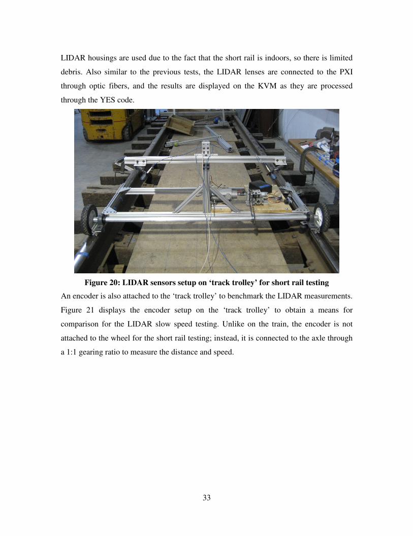
33

LIDAR housings are used due to the fact that the short rail is indoors, so there is limited

debris. Also similar to the previous tests, the LIDAR lenses are connected to the PXI

through optic fibers, and the results are displayed on the KVM as they are processed

through the YES code.

Figure 20: LIDAR sensors setup on ‘track trolley’ for short rail testing

An encoder is also attached to the ‘track trolley’ to benchmark the LIDAR measurements.

Figure 21 displays the encoder setup on the ‘track trolley’ to obtain a means for

comparison for the LIDAR slow speed testing. Unlike on the train, the encoder is not

attached to the wheel for the short rail testing; instead, it is connected to the axle through

a 1:1 gearing ratio to measure the distance and speed.

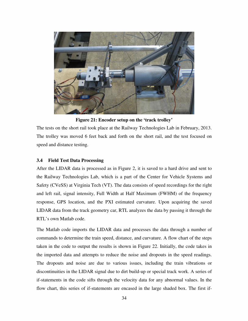
34

Figure 21: Encoder setup on the ‘track trolley’

The tests on the short rail took place at the Railway Technologies Lab in February, 2013.

The trolley was moved 6 feet back and forth on the short rail, and the test focused on

speed and distance testing.

3.4 Field Test Data Processing

After the LIDAR data is processed as in Figure 2, it is saved to a hard drive and sent to

the Railway Technologies Lab, which is a part of the Center for Vehicle Systems and

Safety (CVeSS) at Virginia Tech (VT). The data consists of speed recordings for the right

and left rail, signal intensity, Full Width at Half Maximum (FWHM) of the frequency

response, GPS location, and the PXI estimated curvature. Upon acquiring the saved

LIDAR data from the track geometry car, RTL analyzes the data by passing it through the

RTL’s own Matlab code.

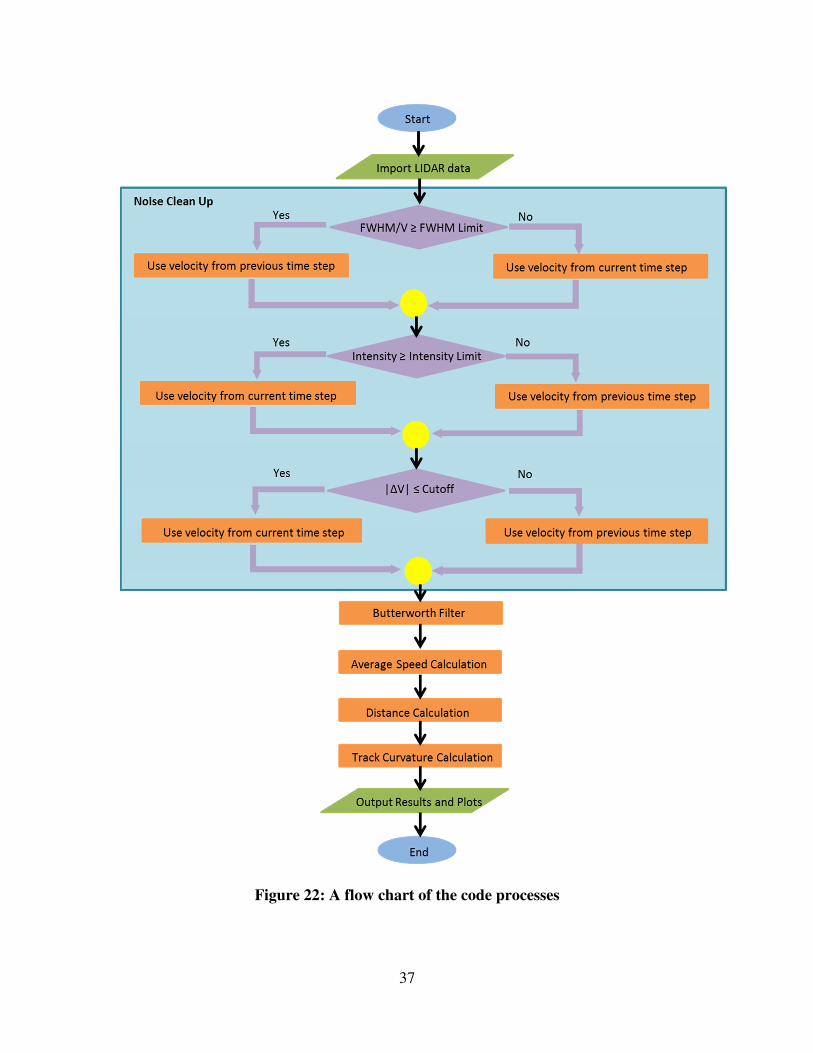
The Matlab code imports the LIDAR data and processes the data through a number of

commands to determine the train speed, distance, and curvature. A flow chart of the steps

taken in the code to output the results is shown in Figure 22. Initially, the code takes in

the imported data and attempts to reduce the noise and dropouts in the speed readings.

The dropouts and noise are due to various issues, including the train vibrations or

discontinuities in the LIDAR signal due to dirt build-up or special track work. A series of

if-statements in the code sifts through the velocity data for any abnormal values. In the

flow chart, this series of if-statements are encased in the large shaded box. The first if-

35

statement assesses the FWHM divided by the velocity for each rail, and if this value is

too large, the current velocity is replaced with the previous velocity. The intensity of each

LIDAR lens is then analyzed over the entire trip. If the intensity is below a certain

threshold, the previous velocity value is utilized. Additionally, change in speed between

the previous speed and the current speed is examined as shown by the following

equation:

|∆�| = |�( − �()�| (5)

where �( is the speed at the present time step, and �()� is the speed from the last time

step. If the change in velocity indicates a sharp change, the preceding velocity reading is

interchanged for the current velocity. The thresholds for each of these if-statements vary

depending on the lens configurations and mounting to properly regulate the data for

irregularities and cleanup the results. The data then passes through a third-order

Butterworth low-pass filter to eliminate any residual noise left from the if-statements.

Once the data is filtered and eradicated of extraneous noise, it is passed through the

equations for speed, distance, and curvature. The following equations are taken or

derived from [55]. The centerline velocity (V) can be calculated with

� =�*+�,

� (6)

where �- is the velocity from the left rail, and �. is the velocity from right rail. The

centerline velocity is the average between the speed readings for each rail throughout the

train trip. The train distance is calculated by using the centerline velocity in the following

equation:

/ = ∑ �( ∗ ∆1((� (7)

in which � is the centerline velocity at a specific data point, ∆1 is the change in time

between data points, and 2 is the total number of data points. Track curvature can be

determined by evaluating the change in speed between the left and right rails with

� =3∗��*)�,�

� (8)

where 4 is an essential scaling factor that varies based on the mounting setup and lens

configuration. This scaling factor is multiplied by the difference between the left and

36

right rail velocity, and then divided by the centerline velocity from Equation (5) to obtain

track curvature. In a curve, the outside rail or high rail travels faster than the inside rail to

compensate for the extra distance. As such, � is positive for right-hand curves and

negative for left-hand curves. An alternate method for computing track curvature is to use

the quarter length analysis method

� =�*∗5

�*)�, (9)

where 6 is the rail gauge, which is generally about 56.5 inches. In this equation, 6 is

assumed to be constant, however, in actuality, the rail gauge fluctuates along the track.

This affects the results of Equation (8), making them less accurate. For this reason, of the

two track curvature equations above, Equation (7) was utilized on the Matlab code.

The code then outputs the results in several plots to display LIDAR-recorded train speed,

distance, and track curvature. The LIDAR results are then compared to encoder and IMU

readings recorded over the same trip.

37

Figure 22: A flow chart of the code processes

38

4 SystemTestResults

4.1 Truck-Mounted LIDAR System Measurements

The test data from the truck-mounted system described in Section 3.3.1 is analyzed for

accuracy in detecting the train speed, distance, and track curvature. Each of these

parameters is then analyzed against standard means of measurements used on track

geometry cars.

4.1.1 Speed Measurements

The LIDAR speed results are compared against the speed calculations derived from the

encoder distance readings. The LIDAR system and the encoder were both attached to the

same track geometry car over the test route mentioned previously. During this trip, the

encoder was installed onto a wheel on the left side of the track geometry car. The encoder

speed measurements were calculated in LabView by multiplying the instantaneous

encoder foot pulse readings and the sampling frequency. In addition to the encoder, a

Global Positioning System (GPS) was also mounted towards the top of the track

geometry car similar to the placement in Figure 5. The encoder and GPS acted as means

for competitive benchmarking.

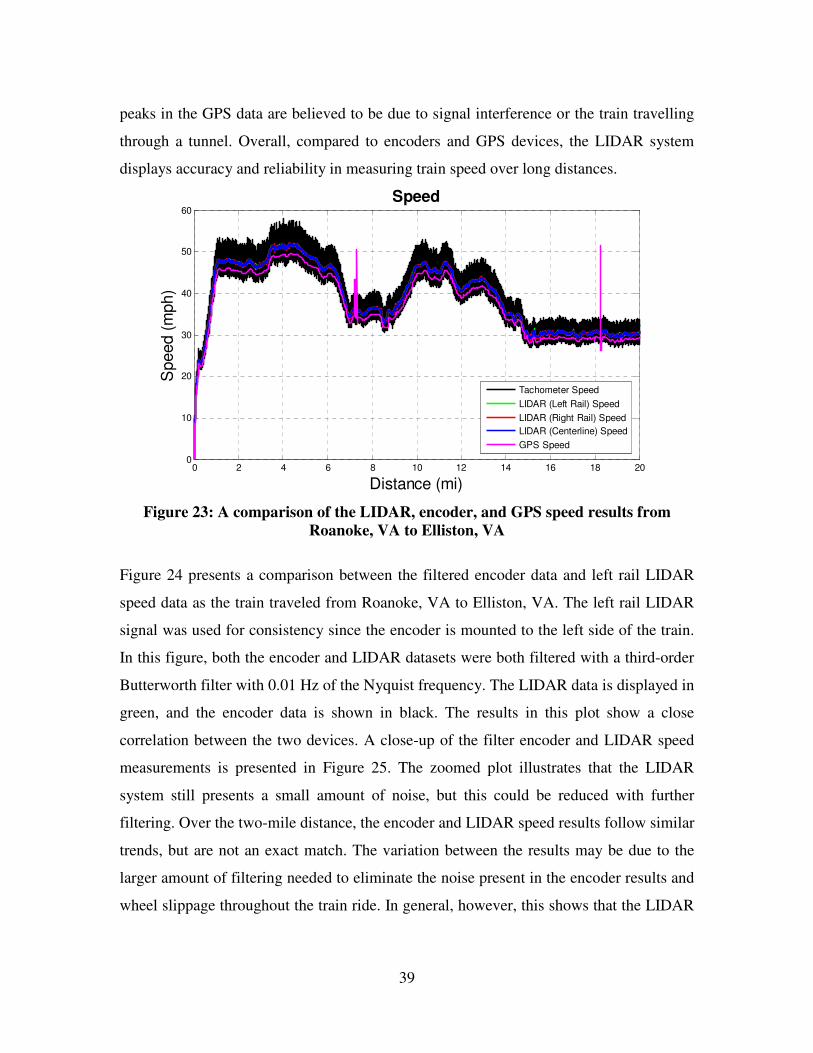
In Figure 23, the left rail, right rail, and centerline LIDAR speed measurements are

compared to the raw encoder and GPS speed measurements. This is shown over a portion

of the truck-mounted trip described earlier, in which the train traveled from Roanoke, VA

to Elliston, VA (approximately 20 miles). All of the devices show similar trends in the

figure, however, the raw encoder data clearly displays large amounts of high frequency

content. In order to increase the accuracy of the encoder on a track geometry car,

encoders are typically set to produce as many as 10,000 pulses per wheel revolution.

Although this increases the accuracy of the encoders, it also increases the likelihood for

the encoder output to contain high signal noise. Generally, the raw encoder data is filtered

significantly to obtain the overall trend of the results. Additionally, the GPS curve

presents areas where the data seems to spike and generate inconsistent results. These

39

peaks in the GPS data are believed to be due to signal interference or the train travelling

through a tunnel. Overall, compared to encoders and GPS devices, the LIDAR system

displays accuracy and reliability in measuring train speed over long distances.

Figure 23: A comparison of the LIDAR, encoder, and GPS speed results from

Roanoke, VA to Elliston, VA

Figure 24 presents a comparison between the filtered encoder data and left rail LIDAR

speed data as the train traveled from Roanoke, VA to Elliston, VA. The left rail LIDAR

signal was used for consistency since the encoder is mounted to the left side of the train.

In this figure, both the encoder and LIDAR datasets were both filtered with a third-order

Butterworth filter with 0.01 Hz of the Nyquist frequency. The LIDAR data is displayed in

green, and the encoder data is shown in black. The results in this plot show a close

correlation between the two devices. A close-up of the filter encoder and LIDAR speed

measurements is presented in Figure 25. The zoomed plot illustrates that the LIDAR

system still presents a small amount of noise, but this could be reduced with further

filtering. Over the two-mile distance, the encoder and LIDAR speed results follow similar

trends, but are not an exact match. The variation between the results may be due to the

larger amount of filtering needed to eliminate the noise present in the encoder results and

wheel slippage throughout the train ride. In general, however, this shows that the LIDAR

0 2 4 6 8 10 12 14 16 18 200

10

20

30

40

50

60

Distance (mi)

Speed (

mph)

Speed

Tachometer Speed

LIDAR (Left Rail) Speed

LIDAR (Right Rail) Speed

LIDAR (Centerline) Speed

GPS Speed

40

system produces speed measurements that are very close to the encoder measurements

over a wide range of speeds.

Figure 24: LIDAR vs. encoder speed from Roanoke, VA to Elliston, VA

Figure 25: A close-up of the LIDAR vs. encoder speed measurements

0 2 4 6 8 10 12 14 16 18 200

10

20

30

40

50

60

Distance (mi)

Speed (

mph)

Speed

Encoder Speed


2 2.2 2.4 2.6 2.8 3 3.2 3.4 3.6 3.8 445

46

47

48

49

50

51

52

53

54

55

Distance (mi)

Speed (

mph)

Speed

Encoder Speed


41

4.1.2 Distance Measurements

The LIDAR distance data was determined by using Equation (5) in Matlab to integrate

the speed data over time. The distance results are then compared to the encoder results as

shown in Figure 26, which displays the distance readings over the same distance and

section of track as shown in Figure 23. The LIDAR distance results for the right, left, and

centerline rails are used to compare against the encoder readings. From the figure, the

LIDAR results appear to be directly overlapping the encoder distance readings. For a

closer comparison, Figure 27 presents a close-up of the distance measurements over a

two-mile distance. The close-up view shows that the distance results from the LIDAR

and encoder readings are extremely close over the two-mile stretch. The two devices do

not appear to slightly diverge until near the four-mile mark. The difference in the distance

measurements is most likely caused by wheel slippage over the tracks, thus affecting the

encoder results. The LIDAR system displays its ability to measure distance with the

same, if not better, accuracy as the encoder.

Figure 26: LIDAR vs. encoder distance from Roanoke, VA to Elliston, VA

0 500 1000 1500 2000 25000

2

4

6

8

10

12

14

16

18

20

Time (s)

Dis

tance (

mi)

Distance

Encoder Distance

LIDAR (Left Rail) Distance

LIDAR (Right Rail) Distance

LIDAR (Centerline) Distance

42

Figure 27: A close-up comparison of the LIDAR vs. encoder distance measurements

4.1.3 Curvature Measurements

The LIDAR results are assessed for ability to measure track curvature accurately. The

curvature results were calculated by using the change in speed between the two wheels,

as mentioned earlier in Equation (6). The track curvature measurements from the truck-

mounted LIDAR system is compared to the Inertial Measurement Unit curvature readings

in Figure 28. This figure displays the track curvature for the same section of track as

shown in Figure 23. The right-hand curves are represented by positive curvatures, and the

left-hand curves are depicted by negatives curvatures.

The IMU and LIDAR curvature data follow similar curvature trends throughout the 20-

mile distance. However, the LIDAR data does show some oscillations in the curvature

measurements. The oscillations could be caused by one or both of the following:

1. The truck experiences yaw throughout the curve, which shifts the relative angle

between the two LIDAR beams and thus generates fluctuations in the curvature

results.

2. The LIDAR system measures curvature with extremely high spatial resolution,

which enables the system to detect local variations in the track geometry. The

IMU measures track curvature based on lateral forces and thus does not pick up

380 400 420 440 460 480 500 5202

2.2

2.4

2.6

2.8

3

3.2

3.4

3.6

3.8

4

Time (s)

Dis

tance (

mi)

Distance

Encoder Distance

LIDAR (Left Rail) Distance

LIDAR (Right Rail) Distance


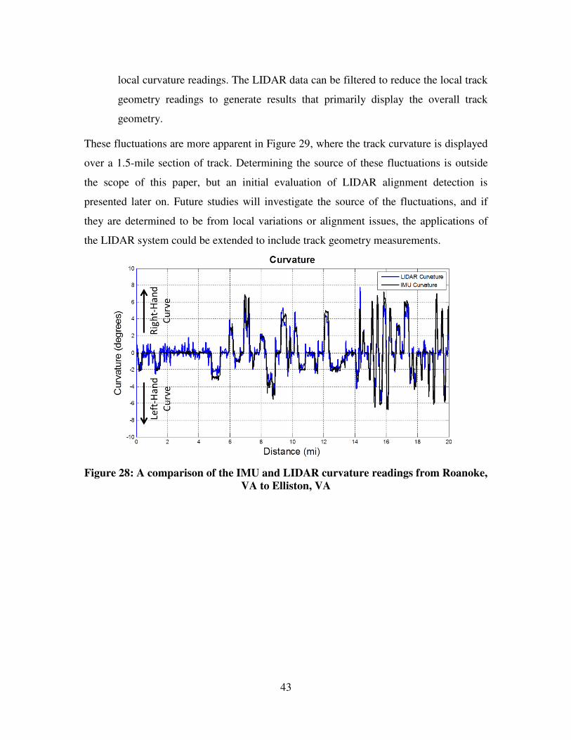
43

local curvature readings. The LIDAR data can be filtered to reduce the local track

geometry readings to generate results that primarily display the overall track

geometry.

These fluctuations are more apparent in Figure 29, where the track curvature is displayed

over a 1.5-mile section of track. Determining the source of these fluctuations is outside

the scope of this paper, but an initial evaluation of LIDAR alignment detection is

presented later on. Future studies will investigate the source of the fluctuations, and if

they are determined to be from local variations or alignment issues, the applications of

the LIDAR system could be extended to include track geometry measurements.

Figure 28: A comparison of the IMU and LIDAR curvature readings from Roanoke,

VA to Elliston, VA

44

Figure 29: The IMU and LIDAR curvature from Roanoke, VA to Elliston, VA over

1.5 mile stretch

The IMU data utilized in Figure 28 and Figure 29 provides the overall track curvature,

but is not an absolute frame of reference for the true track curvature. One way to

accurately measure curvature is to use chord measurements. As mentioned in the

literature review, chord measurements are taken by using a specific length of chord and

stretching the chord ends along the gauge face of the curve. At the mid-point or center of

the chord, the distance from the chord to the gauge face is measured. From this

measurement, the degree curvature can be approximated [42]. In Figure 30, the

relationship between LIDAR, encoder, chordal, and high rail curvature measurements is

assessed. In the figure, the chord measurements are acquired by using a 62ft chord to

measure the curvature by hand. The highrail car measures curvature by taking the average

of the IMU readings over 62ft. The FRA curvature measurements are taken by averaging

10 curvature readings spaced 15.5ft apart (a total of 155ft). The five curvature

measurements in the plot all follow similar trends, but the LIDAR curvature deviates

slightly from the other curvature readings. This could be attributed to the oscillations that

LIDAR senses in curvature readings due to truck yawing or alignment detection.

45

Figure 30: The chordal, FRA, Highrail, IMU, and LIDAR curvature measurements

near Elliston, VA

The LIDAR curvature traveling eastbound and westbound is compared to determine the

repeatability of the LIDAR curvature measurements in Figure 31. The LIDAR curvature

readings traveling westbound and eastbound overlay fairly closely on top of each other.

The biggest deviation between the westbound and eastbound readings occurs at the 7-

mile mark for the 5-degree right-hand curve, and at the 9-mile mark for the 4-degree left-

hand curve. The change in curvature between the westbound and eastbound trip could be

due to differences in truck yawing as the train travels in each direction. Further testing is

necessary to determine if this is the source of the curvature error. A simple solution to

eliminate the deviation in curvature readings is to mount the LIDAR system to the car

body. Since the truck experiences yaw and the car body does not, adjusting the mounting

to the car body could reduce the repeatability errors.

20.94 20.96 20.98 21 21.02 21.04 21.06 21.08 21.1-8

-6

-4

-2

0

2

4

6

8

Distance (mi)

Curv

atu

re (

degre

es)

Curvature

LIDAR Curvature

IMU Curvature

Chord Curvature

Highrail Curvature

FRA Curvature

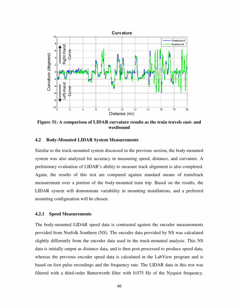
46

Figure 31: A comparison of LIDAR curvature results as the train travels east- and

westbound

4.2 Body-Mounted LIDAR System Measurements

Similar to the truck-mounted system discussed in the previous section, the body-mounted

system was also analyzed for accuracy in measuring speed, distance, and curvature. A

preliminary evaluation of LIDAR’s ability to measure track alignment is also completed.

Again, the results of this test are compared against standard means of train/track

measurement over a portion of the body-mounted train trip. Based on the results, the

LIDAR system will demonstrate variability in mounting installations, and a preferred

mounting configuration will be chosen.

4.2.1 Speed Measurements

The body-mounted LIDAR speed data is contrasted against the encoder measurements

provided from Norfolk Southern (NS). The encoder data provided by NS was calculated

slightly differently from the encoder data used in the truck-mounted analysis. This NS

data is initially output as distance data, and is then post-processed to produce speed data,

whereas the previous encoder speed data is calculated in the LabView program and is

based on foot pulse recordings and the frequency rate. The LIDAR data in this test was

filtered with a third-order Butterworth filter with 0.075 Hz of the Nyquist frequency.

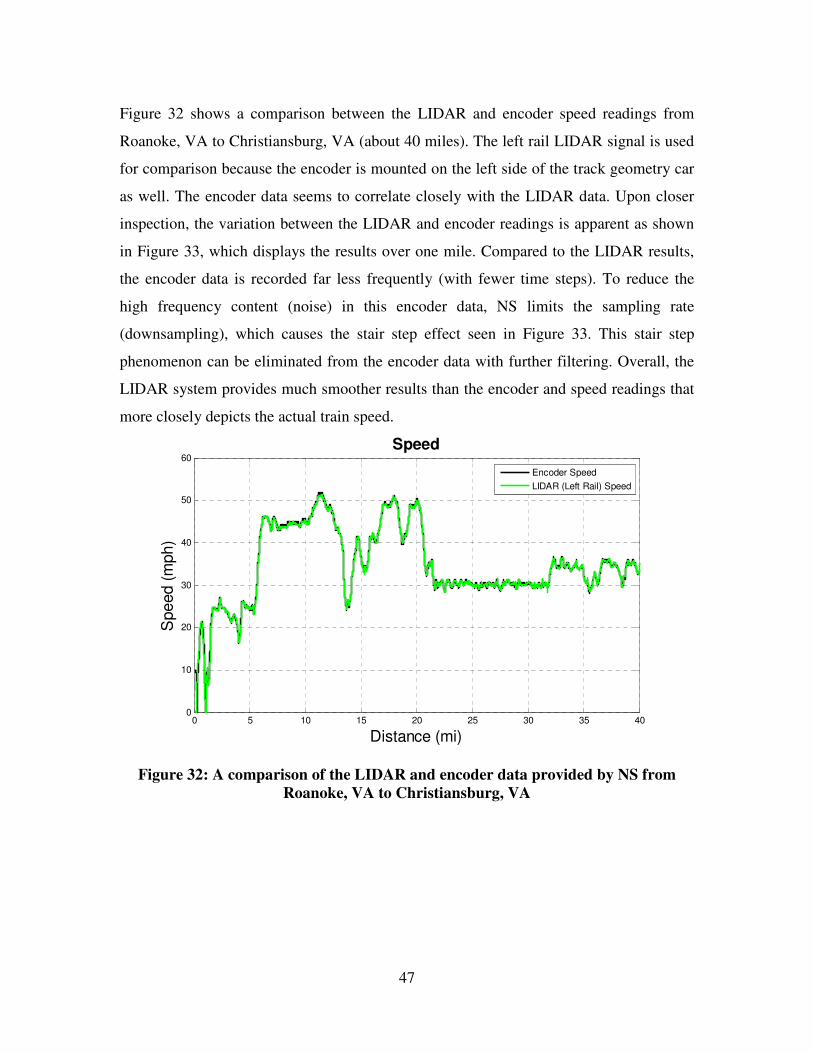
47

Figure 32 shows a comparison between the LIDAR and encoder speed readings from

Roanoke, VA to Christiansburg, VA (about 40 miles). The left rail LIDAR signal is used

for comparison because the encoder is mounted on the left side of the track geometry car

as well. The encoder data seems to correlate closely with the LIDAR data. Upon closer

inspection, the variation between the LIDAR and encoder readings is apparent as shown

in Figure 33, which displays the results over one mile. Compared to the LIDAR results,

the encoder data is recorded far less frequently (with fewer time steps). To reduce the

high frequency content (noise) in this encoder data, NS limits the sampling rate

(downsampling), which causes the stair step effect seen in Figure 33. This stair step

phenomenon can be eliminated from the encoder data with further filtering. Overall, the

LIDAR system provides much smoother results than the encoder and speed readings that

more closely depicts the actual train speed.

Figure 32: A comparison of the LIDAR and encoder data provided by NS from

Roanoke, VA to Christiansburg, VA

0 5 10 15 20 25 30 35 400

10

20

30

40

50

60

Distance (mi)

Speed (

mph)

Speed

Encoder Speed


48

Figure 33: The LIDAR and encoder speed over a one-mile stretch in Glenvar, VA


The body-mounted LIDAR setup is tested for distance measurement accuracy over a

significant number of miles. Again, the LIDAR distance measurements are benchmarked

against the encoder distance measurements in Figure 34. The distance measurements of

the two devices are analyzed for approximately 165 miles from Roanoke, VA to Bristol,

VA. The left rail, right rail, and centerline distance data lie directly on top of each other

and measure a total distance of 165.9 miles. The encoder data diverges significantly from

the LIDAR data and records a total of 202.5 miles. Initially, the LIDAR and encoder are

outputting similar distance measurements for approximately the first 40 miles. Then the

distance measurements of the encoder diverge from the LIDAR measurements as the

train travels farther. Knowing that the train traveled about 165 mile indicates that the

LIDAR system is generating distance measurements far more accurately than the

encoder. The build-up of error in the encoder distance measurements is most likely a

result of wheel slippage, poor encoder calibration, or variations in the wheel diameter.

Figure 35 displays a close-up of the distance measurements in which the encoder displays

small jumps in the distance measurements that are likely due to slippage. This proves that

10.9 11 11.1 11.2 11.3 11.4 11.5 11.6 11.7 11.845

46

47

48

49

50

51

52

53

54

55

Distance (mi)

Speed (

mph)

Speed

Encoder Speed


49

the LIDAR system measures distance more accurately than the encoders currently used

on track geometry cars over long distances and without adjustment.

Figure 34: A comparison of the LIDAR and encoder distance measurements vs. time

for about 165 miles

Figure 35: A close-up of the LIDAR and encoder distance measurements over time

0 0.5 1 1.5 2 2.5 3 3.5

x 104

0

20

40

60

80

100

120

140

160

180

200

Time (s)

Dis

tance (

mi)

Distance

Encoder Distance

LIDAR (Left Rail)Distance

LIDAR (Right Rail)Distance

LIDAR (Centerline Rail)Distance

7500 8000 8500 9000 9500 10000 10500 11000 11500 1200040

45

50

55

60

65

70

75

80

85

90

Time (s)

Dis

tance (

mi)

Distance

Encoder Distance

LIDAR (Left Rail)Distance

LIDAR (Right Rail)Distance

LIDAR (Centerline Rail)Distance

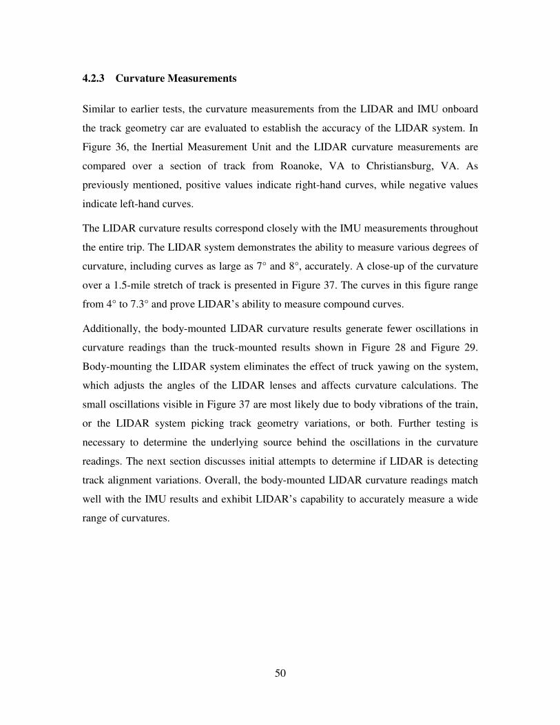
50

4.2.3 Curvature Measurements

Similar to earlier tests, the curvature measurements from the LIDAR and IMU onboard

the track geometry car are evaluated to establish the accuracy of the LIDAR system. In

Figure 36, the Inertial Measurement Unit and the LIDAR curvature measurements are

compared over a section of track from Roanoke, VA to Christiansburg, VA. As

previously mentioned, positive values indicate right-hand curves, while negative values

indicate left-hand curves.

The LIDAR curvature results correspond closely with the IMU measurements throughout

the entire trip. The LIDAR system demonstrates the ability to measure various degrees of

curvature, including curves as large as 7° and 8°, accurately. A close-up of the curvature

over a 1.5-mile stretch of track is presented in Figure 37. The curves in this figure range

from 4° to 7.3° and prove LIDAR’s ability to measure compound curves.

Additionally, the body-mounted LIDAR curvature results generate fewer oscillations in

curvature readings than the truck-mounted results shown in Figure 28 and Figure 29.

Body-mounting the LIDAR system eliminates the effect of truck yawing on the system,

which adjusts the angles of the LIDAR lenses and affects curvature calculations. The

small oscillations visible in Figure 37 are most likely due to body vibrations of the train,

or the LIDAR system picking track geometry variations, or both. Further testing is

necessary to determine the underlying source behind the oscillations in the curvature

readings. The next section discusses initial attempts to determine if LIDAR is detecting

track alignment variations. Overall, the body-mounted LIDAR curvature readings match

well with the IMU results and exhibit LIDAR’s capability to accurately measure a wide

range of curvatures.

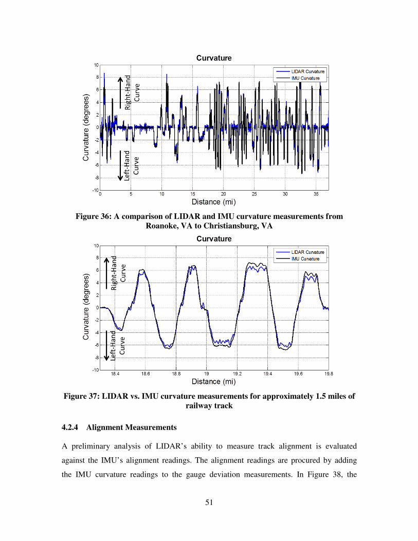
51

Figure 36: A comparison of LIDAR and IMU curvature measurements from

Roanoke, VA to Christiansburg, VA

Figure 37: LIDAR vs. IMU curvature measurements for approximately 1.5 miles of

railway track

4.2.4 Alignment Measurements

A preliminary analysis of LIDAR’s ability to measure track alignment is evaluated

against the IMU’s alignment readings. The alignment readings are procured by adding

the IMU curvature readings to the gauge deviation measurements. In Figure 38, the

52

LIDAR curvature readings are overlaid onto the IMU alignment readings. The IMU

alignment readings show global alignment measurements, which include local track

variation in the curvature. This shows the same section of track as in Figure 37. The

oscillations in the LIDAR curvature display some consistency with the IMU alignment

readings, indicating that the LIDAR system could be detecting track alignment as well as

curvature. Another area of track alignment congruence between the LIDAR and IMU

readings is shown in Figure 39. Any discrepancy between the two alignment results could

be due to the fact that IMU alignment is calculated in a different manner than the LIDAR

data. Additionally, the LIDAR data could be picking up car body vibrations as well as

track alignment. More analysis and testing is needed to differentiate the car body

vibrations in the LIDAR signal from the track alignment. However, the figures following

show promise in LIDAR’s ability to measure track geometry.

Figure 38: A comparison of the LIDAR vs. IMU alignment readings over about 1.5

miles of track

53

Figure 39: A comparison of the LIDAR vs. IMU alignment readings near Wysor,

VA

4.3 Laboratory LIDAR Measurements

The laboratory testing discussed in Section 3.3.3 is analyzed for accuracy in slow speed

and distance measurements. During initial testing, the LIDAR system produced a

significant amount of noise at slow speeds. To resolve this, the sampling rate and a few

other variables in the YES code needed to be adjusted for slow speed testing.

Additionally, a mini-circuit low-pass filtering device is attached directly to the PXI to

filter the data before it is post-processed. The PXI computer with the mini-circuit product

filters circled in red is displayed in Figure 40.

Once the LIDAR system is prepared for slow speed testing, the LIDAR results are

compared to the encoder readings to determine system accuracy. The slow speed LIDAR

system was tested on the ‘track trolley’ (Figure 20), which can be operated by remote

control to move as slowly as 0.25 mph. On a train, encoders typically do not generate

reliable results at low speeds due to slip during acceleration. The hope of these tests is to

demonstrate that LIDAR is capable of recording slow speed measurements accurately,

thus increasing the viability of the LIDAR system.

54

Figure 40: The PXI computer with product filter attachments

4.3.1 Speed Results

The ‘track trolley’ was initially moved by the remote control 6 feet (72 in) along the short

stretch of tangent track rail. The LIDAR slow speed results are evaluated against the

encoder findings in Figure 41. In this figure, the encoder and LIDAR devices are

detecting speeds around 0.3 mph, far below the capabilities of an encoder on a train. The

LIDAR and encoder speeds match closely over the traveled distance, but the LIDAR

results display a bit more noise than the encoder findings. This noise can be reduced,

however, by further filtering the LIDAR results.

An analysis of the system traveling back and forth over 6ft (a total of 144 in) is shown in

Figure 42. Again, the LIDAR and encoder both detect speeds around 0.3 mph and

correlate well overall. It is clear in this figure, however, that encoder data is susceptible to

slip errors when the trolley starts and stops, which leads to the discrepancy in distance

errors. The difference in the distance results will be discussed further in the next section.

In general, this demonstrates LIDAR’s ability to record speeds as small as 0.3 mph

accurately, and shows potential for slow speed testing on the train.

55

Figure 41: A comparison of the left and right rail LIDAR speed results vs. the

encoder speed over 6ft

Figure 42: A comparison of the left and right rail LIDAR speed results vs. the

encoder speed over 12ft


In addition to speed, the LIDAR distance measurements at low speed are analyzed for

accuracy and reliability. The distance measurements are also compared against encoder

0 10 20 30 40 50 60 700

0.05

0.1

0.15

0.2

0.25

0.3

0.35

0.4

0.45

0.5

Distance (in)

Speed (

mph)

Speed

Encoder Speed

LIDAR (Left) Speed

LIDAR (Right) Speed

0 50 100 1500

0.05

0.1

0.15

0.2

0.25

0.3

0.35

0.4

0.45

0.5

Distance (in)

Speed (

mph)

Speed

Encoder Speed

LIDAR (Left) Speed

LIDAR (Right) Speed

56

measurements as a conventional means for distance measurement. Figure 43 displays the

distance measurements over the same distance traveled in Figure 42 (144 in.). Overall,

the distance readings correlate well. Upon closer inspection, as shown in Figure 44, the

encoder is recording slightly higher distance readings as a result of the stop/start slip

errors mentioned earlier. The encoder is recording exactly 150 in. (12.5 ft.), which is an

extra 6 inches over the actual traveled distance of 12 ft. The LIDAR sensors are reading a

total of 148.9 inches, which is about an inch less than the encoder readings. The LIDAR

distance results are still a bit higher than the actual distance, but this may be due to the

oscillations seen in the speed data. By filtering this LIDAR data further, the distance

results would be more accurate. It is also possible that the trolley was moved slightly

more than exactly 12 ft., and that the LIDAR and encoder system are detecting the

additional distance. The results below prove that the LIDAR sensors are able to measure

distance as accurately, if not more accurately, than an encoder.

Figure 43: Encoder vs. LIDAR distance measurements over time

0 10 20 30 40 50 60 700

20

40

60

80

100

120

140

160

Time (s)

Dis

tance (

in)

Distance

Encoder Distance


LIDAR (Left) Distance

LIDAR (Right) Distance

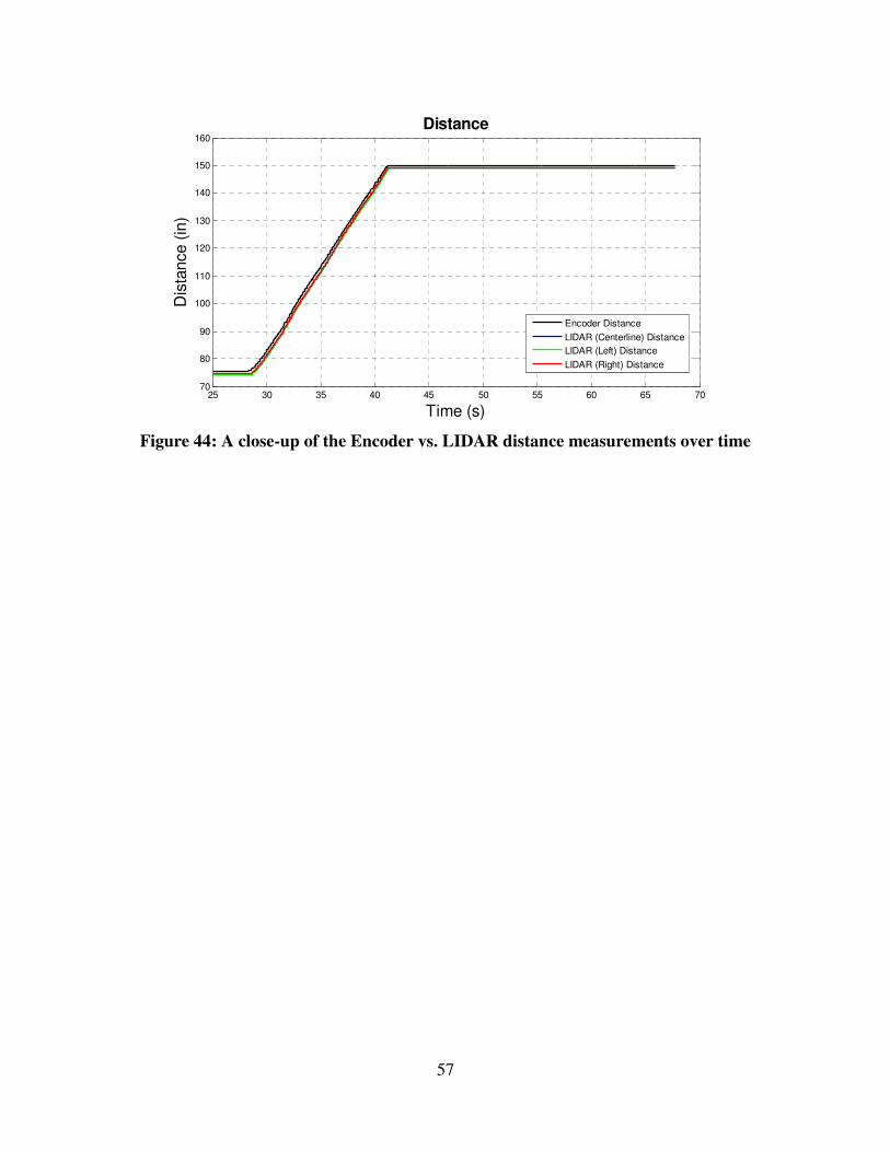
57

Figure 44: A close-up of the Encoder vs. LIDAR distance measurements over time

25 30 35 40 45 50 55 60 65 7070

80

90

100

110

120

130

140

150

160

Time (s)

Dis

tance (

in)

Distance

Encoder Distance


LIDAR (Left) Distance

LIDAR (Right) Distance

58

5 SummaryandConclusion

5.1 Summary

The results of the LIDAR testing performed in this study clearly demonstrate LIDAR’s

applicability and variability for railway applications. As a non-contacting device, LIDAR

eliminates the mechanical, vibrational, and slip errors common with encoders, and it can

also act as a multifunctional measurement device to reduce the need for multiple

measurement devices. The tests demonstrated LIDAR’s ability to measure train speed,

distance, and track curvature at least as accurately as standard wheel-mounted encoders

and IMUs that are currently utilized by the railroad industry. Additionally, LIDAR

generated accurate results over a wider range of speeds than the current track geometry

car equipment. The testing presented LIDAR’s capabilities to measure speeds as slow as

0.3 mph and upwards of 100 mph, whereas most encoders and IMUs become inaccurate

at speeds below 10 mph.

The first test discussed took place on a track geometry car, operated by Norfolk Southern.

The LIDAR system was attached to the truck with the LIDAR lenses facing the top of

rail. A PXI computer with custom-made software was connected to the sensors, which

allowed the system to operate unmanned for a number of weeks. This test focused on

speed, distance, and track curvature measurements, all of which presented good overall

results. The curvature results displayed some oscillating deviations from the IMU

measurements, possibly caused by the truck yawing in curves.

In order to improve the accuracy of the preliminary results, a second test took place on

the track geometry car with the system mounted to the car body and the lenses facing the

gauge corner of the rail. By installing the LIDAR system to the car, the effect of the truck

yawing was eliminated, and the curvature measurements improved. The results of this

test displayed highly accurate speed and distance measurements as compared with the

encoder. There was also a good correlation between the LIDAR and IMU curvature

measurements. Small fluctuations in the LIDAR curvature measurements were still

present, but were significantly reduced from the previous tests. These fluctuations are

most likely caused by car vibrations or variations in track alignment. A preliminary

59

analysis showed the possibility of using LIDAR to measure track geometry, although

further testing is needed.

The final test concentrated on LIDAR’s slow speed and distance measurements. Upon

analyzing the results, it was clear the LIDAR system is capable of accurately measuring

speed and distance at speeds as slow as 0.3 mph. At slow speeds, the acceleration slip

errors in the encoder readings are more apparent and further illustrate the ability of the

LIDAR system to measure speed and distance more accurately than an encoder.

Although the slow speed LIDAR testing showed the presence of noise that slightly

affected the distance measurements, the data can be filtered further in post-processing to

reduce or eliminate the noise.

The overall results of the tests illustrate LIDAR’s capabilities and versatility in measuring

train speed, distance, and track curvature for use on track geometry cars. Further testing,

however, is needed to deduce the root cause of the fluctuations in the curvature

measurements, and to reduce noise during super-slow speed measurements. Conclusively

demonstrating that the curvature variations are caused by track alignment will further

expand LIDAR’s rail applications.

5.2 Conclusions

The significant findings of this study are:

1. A non-contacting LIDAR system is a multi-purpose measurement device that

eliminates the operational issues associated with wheel-mounted encoders, such

as mechanical failures and the need for relatively frequent calibration.

2. LIDAR can accurately measure train speed and distance as compared with

encoders.

3. LIDAR curvature measurements correlate well with IMU curvature

measurements, commonly used on track geometry cars

4. A LIDAR system can be mounted to either the railcar truck or body to acquire

viable measurements.

60

5. A LIDAR system can simultaneously measure speed, distance, and curvature

accurately over an extended range of speeds better than encoders and IMUs, from

speeds as low as 0.3 mph to above 100 mph.

6. Further testing is needed to evaluate the root cause of the fluctuations in the

curvature results.

5.3 Recommendations for Future Studies

Although the results in this study prove that LIDAR is an accurate and reliable system for

railroad applications, it is recommended that further investigation of some of the findings

take place in the near future. In particular, it is recommended that the accuracy, track

geometry detection, and slow speed distance improvements be verified and further

developed, as needed.

The accuracy assessments will include more rigorous tests against known speed, distance,

and curvature measurements. This will allow RTL to further demonstrate the viability of

LIDAR as a multi-functional measurement sensor.

Additional evaluation of variations in curvature measurements is needed to determine the

source and also assess the ability to measure track geometry alignment. Specifically, the

data needs to be analyzed to evaluate the potential for extracting curvature, alignment,

gauge deviation, profile, and super elevation of the track.

LIDAR’s slow speed and distance measurements need to be assessed further in order to

determine the potential for developing a mobile, easy-to-use, track geometry

measurement system. This could be used by railroads to evaluate track conditions similar

to what is commonly performed by track geometry railcars.

61

References

[1] "The Doppler Effect," The Physics Classroom, [Online]. Available:

http://www.physicsclassroom.com/class/waves/u10l3d.cfm. [Accessed 16 December

2012].

[2] W. C. Vantuono, "Do you know where your train is?," Railway Age, vol. 197, no. 2, pp.

41-42, Feb 1996.

[3] POS TG Installation and Operation Manual, Applanix Corporation, 2004.

[4] J. M. Tritthart, "Jeff's Train Site," 13 April 2013. [Online]. Available:

http://www.jeffstrainsite.com/railfan_pics/Class_One/Norfolk_Southern/index.html.

[Accessed 14 April 2013].

[5] U. Wandinger, "Introduction to LIDAR," in LIDAR, vol. 102, Leipzig, Germany,

Springer Series in Optical Sciences, 2005, pp. 1-18.

[6] A. Mirabadi, N. Mort and F. Schmid, "Application of Sensor Fusion to Railway

Systems," in International Conference of Multisensor Fusion for Intelligent Systems,

Washington D.C., 1996.

[7] H. E. Martell, "Applications of Strapdown Inertial Systems in Curvature Detection

Problems," University of Calgary (Canada), Calgary, Alberta, 1991.

[8] J. Trehag, P. Handel and M. Ogren, "Onboard Estimation and Classification of a Railroad

Curvature," IEEE Transactions on Instrumentation and Measurement , vol. 59, no. 3, pp.

653-660, 2010.

[9] W. Middleton and A. Spilhaus, Meteorological Instruments, Toronto: University of

Toronto Press, 1953.

[10] "How does LIDAR work?" [Online]. Available: http://www.lidar-uk.com/how-lidar-

works/ [Accessed 02 March 2013].

[11] "LIDAR-Light Detecting and Ranging," 1 March 2013. [Online]. Available:

https://www.coherent.com/applications/index.cfm?fuseaction=Forms.page&PageID=104.

[Accessed 2 March 2013].

[12] H. Inokuchi, H. Tanaka and T. Ando, "Development of an Onboard Doppler LIDAR for

Flight Safety," in International Congress of the Aeronautical Sciences, Anchorage,

Alaska, 2008.

[13] C. Shun and P. Chan, "Applications of Infared Doppler LIDAR in Detection of Wind

Shear," Journal of Atmospheric and Oceanic Technology, vol. 25, pp. 637-654, 2008.

[14] G. J. Koch, J. Y. Beyon, E. A. Modlin, P. J. Petzar, S. Woll, M. Petro, J. Yu and M. J.

Kavaya, "Side-Scan Doppler LIDAR for Offshore Wind Energy Applications," Journal

of Applied Remote Sensing, vol. 5, pp. 1-11, 2012.

[15] Y. L. Pichugina, R. M. Banta, W. A. Brewer, S. P. Sandberg and R. M. Hardesty,

"Doppler LIDAR-Based Wind-Profile Measurement System for Offshore Wind-Energy

and Other Marine Boundary Layer Applications," Journal of Applied Meteorology and

Climatology, vol. 51, no. 2, pp. 327-349, 2012.

[16] "American Institute of Physics; New Technology May Help Olympic Sailing," China

62

Weekly News, p. 81, 14 July 2008.

[17] D. Pierrottet, F. Amzajerdian, L. Petway, B. Barnes and G. Lackard, "Flight Test

Performance of a High Precision Navigation Doppler LIDAR," in SPIE-The

International Society for Optics and Photonics, 2009.

[18] L. Solomon, "LIDAR: The Speed Enforcement Weapon of Choice," Law Enforcement

Technology, vol. 33, no. 10, pp. 72-76, 2006.

[19] M. Fischetti, "Gotcha!" Scientific American: Working Knowledge, pp. 76-77, 2001.

[20] W. C. McRea, "Measurement of the Speed of a Railway Train by Means of Electro-

Magnetism," Journal of Franklin Institute of the State of Pennsylvania, vol. 62, no. 4, pp.

217-218, 1856.

[21] X. Hongxia, "The Application of Multi-Sensor in Speed Measurement of Location of

Rail Transit," in International Conference on Electronic Measurement and Instruments,

Chengdu, China, 2011.

[22] M. Malvezzi, B. Allotta, M. Bruzzo and P. De Bernardi, "Odometric Estimation for

Automatic Train Protection and Control Systems," Vehicle System Dynamics:

International Journal of Vehicle Mechanics and Mobility, vol. 49, no. 5, pp. 723-739,

2011.

[23] S. S. Saab, G. E. Nasr and E. A. Badr, "Compensation of Axle-Generator Errors Due to

Wheel Slip and Slide," IEEE Transactions on Vehicular Technology, vol. 51, no. 3, pp.

577-587, 2002.

[24] M. Ikeda, "Characteristics of Position Detection and Method of Position Correction by

Rotating Axle," Railway Technical Research Institute, vol. 34, no. 4, pp. 270-276, 1993.

[25] B. Allotta, V. Colla and M. Malvezzi, "Train Position and Speed Esimation Using Wheel

Velocity Measurements," Proceedings of the Institution of Mechanical Engineers:

Journal of Rail and Rapid Transit, vols. 216-225, p. 207, 2002.

[26] Anonynous, "Alaska Moves Toward Safer Operations," Railway Age, vol. 204, no. 6, p.

20, 2003.

[27] Anonymous, "Blending GIS and GPS with Advanced Train Control," Railway Age, vol.

196, no. 3, p. 46, 1995.

[28] T. X. Mei and H. Li, "Measurement of Vehicle Ground Speed Using Bogie-Based

Inertial Sensors," Proceedings of the Institution of Mechanical Engineers. Part F:

Journal of Rail and Rapid Transit, vol. 222, no. 2, pp. 107-116, 2008.

[29] T. X. Mei and H. Li, "A Novel Approach for the Measurement of Absolute Train Speed,"

Vehicle System Dynamics: International Journal of Vehicle Mechanics and Mobility, vol.

46, no. 1, pp. 705-715, 2009.

[30] P. Heide, R. Schubert, V. Magori and R. Schwarte, "A High Performance Multisensor

System for Precise Vehicle Ground Speed Measurement," Microwave Journal, vol. 39,

no. 7, pp. 22-34, 1996.

[31] R. Schubert, P. Heide and V. Magori, "Microwave Doppler Sensors Measuring Vehicle

Speed and Travelled Distance: Realistic System Tests in Railroad Environment," MIOP,

pp. 365-369, 1995.

[32] C. Kakuschke and O. Richter, "Principle Challeneges for Radar Train Speed-over-

63

Ground-Measurement," Frequenz, vol. 60, no. 1-2, pp. 15-19, 2006.

[33] B. Lv, "Design of Velocity Radar for Railway," in International Conference on

Microwave and Millimeter Wave Technology, Chengdu, China, 2010.

[34] T. Engelberg, "Design of a Correlation System for Speed Measurement of Rail

Vehicles," Measurement, vol. 29, no. 2, pp. 157-164, 2001.

[35] A. Geistler, "Train Location with Eddy Current Sensors," in CompRail 2002, Lemnos,

Greece, 2002.

[36] A. Acharya, S. Sadhu and T. Ghoshal, "Train Localization and Parting Detection using

Data Fusion," Transportation Research Part C: Emerging Technologies, vol. 19, no. 1,

pp. 75-84, 2011.

[37] "Biographies of Civil Engineers, Architects, Etc.," SteamIndex, 09 November 2012.

[Online]. Available: http://www.steamindex.com/people/civils.htm#surnha. [Accessed 8

March 2013].

[38] S. Iwnicki, J. Stow and E. Andersson, "Field Testing and Instrumentation of Railway

Vehicles," in Handbook of Railway Vehicle Dynamics, Taylo & Francis Group, 2006, pp.

445-452.

[39] "Horizontal and Vertical Curves," [Online]. Available:

http://www.gisceu.net/PDF/U74.PDF. [Accessed 24 April 2013].

[40] C. F. Allen, "Simple Curves," in Railroad Curves and Earthwork, Norwood, Norwood

Press, 1931, pp. 20-24.

[41] M. Tyler, N. Battjes, N. Plooster, K. Caverly and N. Ovans, "Railroad Surveys: History

and Curve Computation," Ferris State University, [Online]. Available:

http://btcsure1.ferris.edu/bm/documents/Railroad%20Surveys.pdf. [Accessed 8 March

2013].

[42] Railroad Track Standards, Washington DC: Departments of the Army and the Air Force,

1991.

[43] "Traffic Data Collection," Engineering Policy Guide, 19 January 2012. [Online].

Available: http://epg.modot.org/index.php?title=905.1_Traffic_Data_Collection.

[Accessed 24 April 2013].

[44] M. Ahmadian, "Filtering Effects of Mid-Cord Offset Measurement on Track Geometry

Data," in Proceedings of the 1999 ASME/IEEE Joint Railroad Conference, Dallas, TX,

1999.

[45] F. Riewe, "Low-Cost Multiple Sensor Inertial Measurement System for Locomotive

Navigation," ENSCO, Inc. , Cocoa Beach, Fl, 2000.

[46] P. Weston, C. Roberts, C. Goodman and C. Ling, "Condition Monitoring of Railway

Track Using In-Service Trains," in The Institution of Engineering and Technology

International Conference on Railway Condition Monitoring, Birmingham, 2006.

[47] P. Weston, C. Ling, C. Goodman, C. Roberts, P. Li and R. Goodall, "Monitoring Vertical

Track Irregularity from In-Service Railway Vehicles," Institution of Mechanical

Engineers Part F: Journal of Rail and Rapid Transport, vol. 221, no. 1, pp. 75-88, 2007.

[48] A. M. Boronakhin, L. N. Podgornaya, E. D. Bokhman, N. S. Filipenya, V. Yu and R. B.

Filatov, "MEMS-Based Inertial System for Railway Track Diagnostics," Gyroscopy and

64

Navigation, vol. 2, no. 4, pp. 261-268, 2011.

[49] M. Trosino, "Developments and Applications in the Amtrak Track Geometry

Measurement Car," in The International Society for Optics and Photonics:

Nondestructive Evaluaion of Aging Railroads, Oakland, CA, 1995.

[50] D. Jamieson, J. Bloom and R. Kelshaw, "T-2000: A Railroad Track Geometry Inspection

Vehicle for the 21st Century," in Proceedings of American Railway Engineering and

Maintenance-of-Way Association Conference, Chicago, Illinois, 2001.

[51] F. Leahy, M. Judd and M. Shortis, "Measurement of Railway Profiles Using GPS

Integrated with Other Sensors," in Proceedings of IEEE: Vehicle Navigation and

Information Systems Conference, Ottawa, Ontario, 1993.

[52] I. Hans-Jurgen Euler and C. D. Hill, "Real-Time Precise GPS for Railroad Mapping," in

Proceedings of IEEE: Position Location and Navigation Symposium, Atlanta, GA, 1996.

[53] O. Heirich, A. Lehner, P. Robertson and T. Strang, "Measurement and Analysis of Train

Motion and Railway Track Characteristics with Inertial Sensors," in 14th International

Conference on Intelligent Transport Systems, Washington D.C., 2011.

[54] N. Atamanov, V. Troitskiy, I. Gusev, V. Korotin and P. Kuleshov, "Railway Track

Inspection Using INS-BINS-N," IEEE Aerospace and Electronic Systems Magazine, vol.

22, no. 3, pp. 30-34, 2007.

[55] C. Holton and M. Ahmadian, "Doppler Sensor for the Derivation of Torsional Slip,

Friction and Related Parameters." United States Patent 7,705,972, 27 April 2010.

Documents

MULTI-FUNCTION LIDAR SENSORS FOR NON-CONTACT …