Embed Size (px)
Citation preview

Multi-Aspect Temporal Network Embedding:A Mixture of Hawkes Process View
Yutian Chang
School of Economics and Management
Beihang University
Beijing 100191, China
Guannan Liu∗
School of Economics and Management
Beihang University
Beijing 100191, China
Yuan Zuo
School of Economics and Management
Beihang University
Beijing 100191, China
Junjie Wu†
School of Economics and Management
Beijing Advanced Innovation Center for Big Data and
Brain Computing
Beihang University
Beijing 100191, China
ABSTRACTRecent years have witnessed the tremendous research interests in
network embedding. Extant works have taken the neighborhood
formation as the critical information to reveal the inherent dynam-
ics of network structures, and suggested encoding temporal edge
formation sequences to capture the historical influences of neigh-
bors. In this paper, however, we argue that the edge formation can
be attributed to a variety of driving factors including the temporal
influence, which is better referred to as multiple aspects. As a matter
of fact, different node aspects can drive the formation of distinctive
neighbors, giving birth to the multi-aspect embedding that relates
to but goes beyond a temporal scope. Along this vein, we propose a
Mixture of Hawkes-based Temporal Network Embeddings (MHNE)
model to capture the aspect-driven neighborhood formation of net-
works. In MHNE, we encode the multi-aspect embeddings into the
mixture of Hawkes processes to gain the advantages in modeling
the excitation effects and the latent aspects. Specifically, a graph
attention mechanism is used to assign different weights to account
for the excitation effects of history events, while a Gumbel-Softmax
is plugged in to derive the distribution over the aspects. Extensive
experiments on 8 different temporal networks have demonstrated
the great performance of the multi-aspect embeddings obtained by
MHNE in comparison with the state-of-the-art methods.
CCS CONCEPTS• Information systems→ Data mining; Network data models; •Computingmethodologies→Dimensionality reduction andmanifold learning.
∗Corresponding author
†Also with , Beijing Key Laboratory of Emergency Support Simulation Technologies
for City Operations, Beihang University.
Conference’17, July 2017, Washington, DC, USA2021. ACM ISBN 978-x-xxxx-xxxx-x/YY/MM. . . $15.00
https://doi.org/10.1145/nnnnnnn.nnnnnnn
KEYWORDSNetwork embedding, Hawkes process, Multi-aspect, Temporal net-
work
ACM Reference Format:Yutian Chang, Guannan Liu, Yuan Zuo, and Junjie Wu. 2021. Multi-Aspect
Temporal Network Embedding: A Mixture of Hawkes Process View. In
Proceedings of ACM Conference (Conference’17). ACM, New York, NY, USA,
11 pages. https://doi.org/10.1145/nnnnnnn.nnnnnnn
1 INTRODUCTIONNetwork embedding has attracted extensive attentions in recent
years due to its efficiency in encoding network structure into low
dimensional representations [3, 7, 8, 19, 20], which can be flexibly
applied to various downstream tasks. In addition to embedding
static networks, some efforts have also been made to tackle the
dynamic evolving structure of temporal networks [4, 6, 13, 17, 26].
Conventional temporal network embedding methods [6, 17] model
the network dynamics via multiple snapshots derived from different
time periods, which can only represent the network structure in a
certain time window. To overcome the limitations of the snapshot-
based methods, recent work [13, 26] has attempted to track the
neighborhood formation sequence of each node, where the connec-
tion between a target node and the source node primarily depends
on the similarity between the two nodes and the influence of the
historical target nodes. In this regard, a complete temporal pro-
cess of network formation can be revealed and hence the derived
embeddings can reflect the evolution patterns of nodes.
However, except for the temporal view of the neighborhood for-
mation, as a matter of fact, the connections between a source node
and its target nodes may be driven by different underlying factors,
which can be referred to as aspects. The aspects of nodes can have
different meanings in terms of different networks. Especially, the
aspects may change over time, and therefore can induce distinctive
neighborhood formation of a node. For example, assume that node
𝑢 in Fig. 1 is a researcher who focused on Database (DB) at theearly stages and then shifts his interest to Artificial Intelligence (AI).The left part of the Fig. 1 illustrates the historical coauthors of 𝑢
arX
iv:2
105.
0856
6v1
[cs
.LG
] 1
8 M
ay 2
021

Conference’17, July 2017, Washington, DC, USA Yutian Chang, Guannan Liu, Yuan Zuo, and Junjie Wu
DB
AI
?𝑢𝑢
𝑣𝑣1
𝑣𝑣2
𝑡𝑡
Probability of 𝑢𝑢 collaborating with researchers from different fields
𝜋𝜋𝑢𝑢(𝑡𝑡2)
DB AI
𝜋𝜋𝑢𝑢(𝑡𝑡1)
DB AI
Figure 1: An example of considering the history sequenceand multiple aspects of nodes
listed chronologically on the x-axis, where the y-axis denotes the
probability of node 𝑢 collaborating with researchers from different
fields (i.e., aspects). The blue/red line in the figure represents the
activeness of 𝑢 in terms of DB/AI, as illustrated, the blue line has
a clear downward trend while the red one keeps rising over time.
Therefore, given two nodes 𝑣1 and 𝑣2 representing researchers who
are currently focusing on AI and DB respectively, we can easily
infer that 𝑢 has a larger chance of establishing co-authorship with
𝑣1 than 𝑣2 according to 𝑢’s neighborhood sequence. In contrast,
from a static point of view as shown on the rightmost part of Fig. 1,
where the neighbors of 𝑢 are regard as an unordered static node
set, future connections of 𝑢 are much less predictable. As seen from
the example, the formation of temporal edges are indeed driven by
different aspects of nodes, which is essential to understand the un-
derlying mechanism of network evolution. However, prior temporal
network embedding methods generally derive a single embedding
for each node, and merely address different node aspects.
Given that nodes in networks may have multiple aspects, several
prior work [5, 12, 18, 22, 23] has attempted to represent each node
with multiple embeddings. Compared to a single embedding vector,
multiple embeddings enlarges the embedding space, with each
embedding exclusively focusing on one specific aspect. However,
these multi-aspect embeddings are derived from a static network,
which indeed has some inherent limitations. On the one hand, the
neighborhood of a node is generally modeled as an unordered node
set, where neighbors that formed at distant timestamps would not
be treated differently, thus the derived multi-aspect embedding
may simply be an aggregated distribution over the aspects of all
the neighbors. On the other, the node aspects can change over
time, and there might be a focal aspect at one time but the static
view fails to capture this. Thus, it cannot precisely predict the
future neighbor formation with the out-dated aspect information.
Apparently, the temporal network setting is more desirable for
multi-aspect embeddings. As a matter of fact, temporal network
embedding and the multi-aspect embedding can indeed be regarded
as the two sides of a coin and should complement with each other.
As far as we are concerned, we are among the first to take a temporal
view to derive the multi-aspect embeddings.
To tackle the above-mentioned challenges, we extend the neigh-borhood formation to a notion of aspect driven edge formation by
plugging an aspect distribution for each edge formed at specific
time to account for the aspect-drive factors, which gives rise to a
Multi-Aspect Temporal Network. In order to obtain the multi-aspect
embedding from the temporal network, we propose an end-to-
end method named Mixture of Hawkes-based Temporal NetworkEmbedding (MHNE) in this paper. In overall, we model the aspect-
driven neighborhood formation with a mixture of Hawkes process
(MHP) [24], which has great merits in capturing both the temporal
excitation effects of historical events and the latent aspects within
the sequence. In particular, we exploit the MHP to model the edge
formation probability by feeding the multi-aspect embeddings into
the intensity function. More specifically, the aspect distribution
is induced via Gumbel-Softmax [9] with a trainable temperature
parameter that controls the extent to which we desire a one-hot
alike distribution. Additionally, graph attention mechanism [21] is
incorporated to assign different weights to the excitation effects
of history events. We have conducted extensive experiments on
eight different real-world networks by utilizing the the multi-aspect
embeddings for several downstream including link prediction, tem-
poral node recommendation. The experimental results have demon-
strated the superiority of MHNE over the state-of-the-art methods,
and we have also rigorously validated the effectiveness the model-
ing components, especially the quality of aspects.
2 PRELIMINARY2.1 Aspect Driven Neighborhood FormationRecent works [13, 25] try to learn temporal network embedding by
looking into the formation process of the network, specifically, the
neighborhood formation process of nodes. However, as illustrated
in the toy example, they ignore a fact that the evolution of edges are
inherently driven by the underlying aspects, which provides a more
comprehensive view of the neighborhood formation process. Based
on the above consideration, we formally define the multi-aspect
temporal network.
Definition 1 (Multi-Aspect TemporalNetwork). Multi-aspecttemporal network is a network with aspects driven temporal edges,which can be denoted as G =< V, E;H ,K >, where V denotesthe set of nodes, E denotes the set of temporal edges,H denotes theset of neighborhood formation sequences and K denotes the set ofaspect distributions. Each temporal edge 𝑒 = (𝑢, 𝑣, 𝑡) ∈ E betweenthe source node 𝑢 and the target node 𝑣 at time 𝑡 is driven by theaspect distribution K𝑢 (𝑡) and the neighborhood formation sequenceH𝑢 (𝑡) = {(ℎ, 𝑡ℎ) | (𝑢,ℎ, 𝑡ℎ) ∈ E, 𝑡ℎ < 𝑡} of the source node 𝑢.
From the above definition, we can find the evolution of edges
in the multi-aspect temporal network is still modeled with neigh-
borhood formation sequence of the source node. The difference
is the evolution of edges is also driven by the unobserved aspect
distribution of the source node, with which a much clearer clue
is provided for predicting future connections of the source node.
Therefore, we formally define the aspect driven edge formation.
Definition 2 (Aspect Driven Edge Formation). Given a tem-poral edge 𝑒 = (𝑢, 𝑣, 𝑡) and the neighborhood formation sequenceH𝑢 (𝑡) of its source node 𝑢 at time 𝑡 , the formation probability of𝑒 , in other words, the probability of 𝑢 connecting to 𝑣 at time 𝑡 is𝑝 (𝑣 |𝑢, 𝑡,H𝑢 (𝑡)). Given the aspect distribution K𝑢 (𝑡) of the sourcenode 𝑢 at time 𝑡 , the formation probability of temporal edge 𝑒 driven
Multi-Aspect Temporal Network Embedding:A Mixture of Hawkes Process View Conference’17, July 2017, Washington, DC, USA
by the aspects can be decomposed as:
𝑝 (𝑣 |𝑢, 𝑡,H𝑢 (𝑡)) =|K𝑢 (𝑡 ) |∑︁𝑘=1
K𝑘𝑢 (𝑡)𝑝 (𝑣 |𝑢, 𝑡,H𝑢 (𝑡), 𝑘), (1)
whereK𝑘𝑢 (𝑡) = 𝑝 (𝑘 |𝑢, 𝑡) is the probability of 𝑘-th aspect of the source
node 𝑢 at time 𝑡 , 𝑝 (𝑣 |𝑢, 𝑡,H𝑢 (𝑡), 𝑘) is the formation probability of 𝑒driven by the neighborhood formation sequenceH𝑢 (𝑡) and the 𝑘-thaspect.
With the aspect driven edge formation defined above, we can eas-
ily understand how the neighborhood formation sequenceH𝑢 (𝑡)of the source node 𝑢 is driven by its aspects distribution K𝑢 (𝑡).That is, for each pair of history target node ℎ and timestamp ℎ𝑡 in
H𝑢 (𝑡), there is an edge (𝑢,ℎ, 𝑡ℎ) that is driven by K𝑢 (𝑡). Once allnodes’ neighborhood formation sequences at all timestamps are
driven by the aspects, the entire multi-aspect temporal network
will be established.
2.2 Problem DefinitionGiven a multi-aspect temporal network G =< V, E;H ,K >, the
neighborhood formationH𝑢 (𝑡) of each node𝑢 ∈ V can be induced
by tracking all the timestamps when 𝑢 interacts with its neighbors
before time 𝑡 . However, the aspect distribution K𝑢 (𝑡) of each node
𝑢 at time 𝑡 is unobserved. To learn multiple aspects that driven
the entire temporal network, we resort to learn the multi-aspect
temporal network embedding as defined in the follow.
Definition 3 (Multi-Aspect Temporal Network Embedding).
Given the multi-aspect temporal network G =< V, E;H ,K >, weaim to learn an embedding function 𝜙 : 𝑢 ∈ V → {I𝑢 ∈ R𝑚,A𝑢 ∈R𝐾∗𝑚}, where I𝑢 is the identity embedding of node 𝑢, and A𝑘𝑢 rep-resents the embedding of 𝑘-th aspect of node 𝑢, 𝐾 is the number ofaspects, and𝑚 is the embedding size satisfies𝑚 ≪ |V|.
With the learned embeddings, probabilities in Eq. 1 can be com-
puted in a straightforward manner as described in Sect. 3.2. There-
fore, the underlying aspects in the temporal network can be re-
vealed. Note that the learning of multiple aspects and the temporal
network embedding are actually complement each other. Especially,
we emphasize that the temporal networks are more suitable for
multi-aspect embedding learning than the static network for the
detailed information in the formation process of temporal networks
is essential to induce node aspects.
3 METHODOLOGY3.1 Hawkes ProcessHawkes process is a typical temporal point process in modeling
discrete events considering the temporal decay effect of history
events, whose conditional intensity function is defined as follows,
_(𝑡) = ` (𝑡) +∫ 𝑡
−∞J (𝑡 − 𝑠)d𝑁 (𝑠), (2)
where ` (𝑡) is the base intensity of a particular event, showing the
spontaneous event arrival rate at time 𝑡 , J (·) is a kernel functionthat models the time decay effect of history events on the current
event, which is usually in the form of an exponential function, and
𝑁 (𝑠) denotes the number of events until time 𝑠 .
The conditional intensity function of Hawkes process shows that
the occurrence of current event does not only depend on the event
of last time step, but is also influenced by the historical events
with time decay effect. Such property is desirable for modeling
the neighborhood formation sequences, for the current neighbor
formation can be influenced with higher intensity by the more
recent events.
To model the evolution of an edge based on its source node’s var-
ious neighbor nodes, multivariate Hawkes process is adopted [26],
that is,
_𝑑 (𝑡) = `𝑑 (𝑡) +𝐷∑︁𝑑′=1
∫ 𝑡
−∞J𝑑′𝑑 (𝑡 − 𝑠)d𝑁𝑑′ (𝑠), (3)
where the conditional intensity function is designed for each event
type as one dimension, such as the𝑑 or𝑑 ′ dimension. The excitation
effects are indeed a sum over all the historical events with different
types, captured by an excitation rate 𝛼𝑑′,𝑑 between dimension 𝑑
and 𝑑 ′, formally, J𝑑′𝑑 (𝑡 − 𝑠) = 𝛼𝑑′𝑑J (𝑡 − 𝑠).When modeling multi-aspect temporal network, the neighbor-
hood formation sequence can be further decomposed into multiple
event sequences according to their underlying aspects. Therefore
we resort to the Mixture of Hawkes Process (MHP), where event se-
quences driven by various aspects can be modeled simultaneously.
Suppose that there are 𝐾 different aspects that driven the occur-
rence of current event (i.e. edge), each aspect can be modeled as
a component of the MHP. Extended from the Eq. 3, we have the
intensity function of the current event motivated by aspect 𝑘 as
follows,
_𝑘𝑑(𝑡) = `𝑘
𝑑(𝑡) +
𝐷∑︁𝑑′𝛼𝑘𝑑′𝑑
∫ 𝑡
−∞J (𝑡 − 𝑠)d𝑁𝑘
𝑑′ (𝑠), (4)
where `𝑘𝑑(𝑡) denotes the base intensity on current event 𝑑 excited
by the 𝑘-th aspect, 𝑁𝑘𝑑(𝑡) is the number of events that driven by the
𝑘-th aspect until time 𝑡 , 𝛼𝑘𝑑′𝑑
denotes the mutual excitation effect
between dimension 𝑑 ′ and 𝑑 in terms of the 𝑘-th aspect. Therefore
the intensity function of MHP is _𝑑 (𝑡) = 𝜋𝑘_𝑘𝑑 (𝑡), where 𝜋𝑘is the
mixture weight.
3.2 Mixture of Hawkes based temporalNetwork Embedding
As discussed above, we firstly model the aspect driven neighbor-
hood formation sequences via Mixture of Hawkes Process (MHP),
which is then adapted to learn embeddings. In this way, we can
tackle the multi-aspect temporal network embedding problem. Now
we formally propose our model named Mixture of Hawkes tempo-
ral Network Embedding (MHNE).
Assume there are 𝐾 aspects in the multi-aspect temporal net-
work, the intensity function of the MHP for node 𝑣 connecting to
node 𝑢 at time 𝑡 can be written as,
_𝑣 |𝑢 (𝑡) =∑︁𝑘
𝜋𝑘𝑢 (𝑡)_𝑘𝑣 |𝑢 (𝑡), (5)
where 𝜋𝑘𝑢 (𝑡) denotes the probability of node𝑢 driven by 𝑘-th aspect
at time 𝑡 (i.e., the mixture weight of 𝑘-th aspect), _𝑘𝑣 |𝑢 (𝑡) denotes the
Conference’17, July 2017, Washington, DC, USA Yutian Chang, Guannan Liu, Yuan Zuo, and Junjie Wu
𝐂𝐂𝑢𝑢 𝑡𝑡
𝐀𝐀
𝐈𝐈
: ℎ5𝑣𝑣 𝑢𝑢 ℎ1
ℎ2
ℎ3
ℎ4
ℎ5
Aspect distribution and parameter calculation Mixture of Hawkes process
…𝜆𝜆𝑣𝑣|𝑢𝑢(𝑡𝑡)+
𝜋𝜋ℎ𝑖𝑖3 (𝑡𝑡)
𝓘𝓘(·)
𝛼𝛼ℎ𝑖𝑖,𝑣𝑣 𝛾𝛾ℎ𝑖𝑖,𝑣𝑣3
𝛼𝛼ℎ𝑖𝑖,𝑣𝑣3
𝜇𝜇𝑢𝑢,𝑣𝑣 𝛾𝛾𝑢𝑢,𝑣𝑣3
𝜇𝜇𝑢𝑢,𝑣𝑣3
+×
× ×
𝜆𝜆𝑣𝑣|𝑢𝑢3 (t)
𝜋𝜋𝑢𝑢3(𝑡𝑡)×
𝜋𝜋ℎ𝑖𝑖1 (𝑡𝑡)
𝓘𝓘(·)
𝛼𝛼ℎ𝑖𝑖,𝑣𝑣 𝛾𝛾ℎ𝑖𝑖,𝑣𝑣1
𝛼𝛼ℎ𝑖𝑖,𝑣𝑣1
𝜇𝜇𝑢𝑢,𝑣𝑣 𝛾𝛾𝑢𝑢,𝑣𝑣1
𝜇𝜇𝑢𝑢,𝑣𝑣1
+×
× ×
𝜆𝜆𝑣𝑣|𝑢𝑢1 (t)
𝜋𝜋𝑢𝑢1(𝑡𝑡)×
𝐻𝐻
𝐻𝐻
ℎ4ℎ3ℎ2ℎ1
Gumbel-Softmax
ℱ
𝑣𝑣
-ℱ-ℱ
ℱ
𝛼𝛼ℎ,𝑣𝑣𝜇𝜇𝑢𝑢,𝑣𝑣
-ℱ
-ℱ
𝛾𝛾ℎ𝑖𝑖 ,𝑣𝑣𝑘𝑘𝛾𝛾𝑢𝑢,𝑣𝑣
𝑘𝑘 𝛾𝛾ℎ𝑖𝑖,𝑣𝑣𝑘𝑘𝛾𝛾𝑢𝑢,𝑣𝑣
𝑘𝑘
Graph Attention
Occurrence Intensity
𝝅𝝅𝒏𝒏(t)
𝝅𝝅𝒏𝒏𝟏𝟏(𝒕𝒕)𝝅𝝅𝒏𝒏𝟐𝟐(𝒕𝒕)𝝅𝝅𝒏𝒏𝟑𝟑(𝒕𝒕)
Occurrence Intensity
𝑢𝑢
Excitation effect of history nodes Rate of 𝒖𝒖 connecting with 𝒗𝒗
Mixture component of MHP
Mixture weight
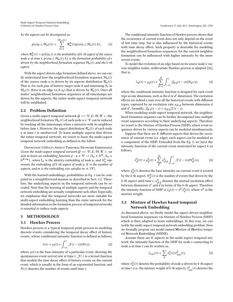
Figure 2: Framework of MHNE
intensity of node 𝑣 connects with 𝑢 at time 𝑡 driven by 𝑘-th aspect,
which is a intensity function of multivariate Hawkes process.
Recall the Definition 2, given the aspect distributionK𝑢 (𝑡) of thesource node𝑢, the the probability 𝑝 (𝑣 |𝑢, 𝑡,H𝑢 (𝑡)) that𝑢 connects to𝑣 at time 𝑡 can be written as Eq. (1). By comparing Eq. (1) and Eq. (5),
it is not hard to find that 𝜋𝑘𝑢 (𝑡) and _𝑘𝑣 |𝑢 (𝑡) are analog to theK𝑢 (𝑡)and 𝑝 (𝑣 |𝑢, 𝑡,H𝑢 (𝑡), 𝑘) in Eq. (1) respectively, which indicates the
MHP intensity function defined above is modeling the aspect driven
edge formation. Therefore, the MHP has potential to be adapted to
tackle the multi-aspect temporal network embedding problem. In
the following, we show how to adapt the MHP with multi-aspect
embeddings, by firstly describing how to adapt the _𝑘𝑣 |𝑢 (𝑡), then
presenting how to obtain the aspect distribution 𝜋𝑘𝑢 (𝑡).Adapted Intensity Function. The intensity _𝑘
𝑣 |𝑢 (𝑡) can be formu-
lated according to Eq. (4), that is,
_̃𝑘𝑣 |𝑢 (𝑡) = `
𝑘𝑢,𝑣 +
∑︁ℎ∈H𝑢 (𝑡 )
𝜋𝑘ℎ(𝑡)𝛼𝑘
ℎ,𝑣J (𝑡 − 𝑡ℎ), (6)
where `𝑘𝑢,𝑣 denotes the rate of node 𝑢 connects to 𝑣 motivated by 𝑘-
th aspect, ℎ denotes the historical nodes connected to 𝑢 before time
𝑡 , 𝛼𝑘ℎ,𝑣
denotes the excitation effect of history node ℎ on target node
𝑣 and 𝜋𝑘ℎ(𝑡) denotes the activeness of node ℎ on 𝑘-th aspect. The
`𝑘𝑢,𝑣 can be further decomposed into the base rate `𝑢,𝑣 that node 𝑢
and node 𝑣 connecting with each other, and the excitation effect
𝛾𝑘𝑢,𝑣 from 𝑘-th aspect. Then, we have `𝑘𝑢,𝑣 = `𝑢,𝑣𝛾𝑘𝑢,𝑣 . Similarly, 𝛼𝑘
ℎ,𝑣
can be decomposed into 𝛼ℎ,𝑣𝛾𝑘ℎ,𝑣
. Based on above consideration,
Eq. (6) is rewritten as,
_̃𝑘𝑣 |𝑢 (𝑡) = `𝑢,𝑣𝛾
𝑘𝑢,𝑣 +
∑︁ℎ∈H𝑢 (𝑡 )
𝜋𝑘ℎ(𝑡)𝛼ℎ,𝑣𝛾𝑘ℎ,𝑣J (𝑡 − 𝑡ℎ), (7)
where J (𝑡 − 𝑡ℎ) = exp(−𝛿𝑢 (𝑡 − 𝑡ℎ)) is the kernel function models
time decay effect. Since the influence extent of history can be vari-
ous between different nodes, we introduct a trainable parameter
𝛿𝑢 for each node.
Intuitively, the probability that two nodes connect with each
other are proportion to their similarity. Thus we define a function
F : R𝑑 → R that maps the embeddings of two corresponding
nodes into a similarity score, with which, we are able to adapt the
intensity _𝑘𝑣 |𝑢 with embeddings. Specifically, we show `𝑢,𝑣 , 𝛼ℎ,𝑣 can
be computed via F as
`𝑢,𝑣 = F (I𝑢 , I𝑣), (8)
𝛼ℎ,𝑣 = F (Iℎ, I𝑣), (9)
where I𝑢 , I𝑣 and Iℎ are identity embeddings of node 𝑢, node 𝑣
and node ℎ, respectively. Although there are many choices, we
empirically find that negative Euclidean distance works the best.
Therefore, F (𝑥,𝑦) = − ∥𝑥 − 𝑦∥2, where 𝑥 and 𝑦 are node embed-
dings.
Similarly, 𝛾𝑘𝑢,𝑣 and 𝛾𝑘ℎ,𝑣
can be computed via F as
𝛾𝑘𝑢,𝑣 = −F (A𝑘𝑢 ,A𝑘𝑣 ), (10)
𝛾𝑘ℎ,𝑣
= −F (A𝑘ℎ,A𝑘𝑣 ), (11)
where A𝑘𝑢 , A𝑘𝑣 and A𝑘
ℎare aspect embeddings. Notably, in order
to maintain the monotonicity of `𝑘𝑢,𝑣 and 𝛼𝑘ℎ,𝑣
, a negative sign is
added before F .
Finally, the intensity function _𝑘𝑣 |𝑢 (𝑡) can be parameterized with
the embedding matrices {I,A}. Since intensity function should
take positive value when regarded as a rate per unit time, we apply
exp(·) to convert _̃𝑘𝑣 |𝑢 (𝑡) into positive value, that is,
_𝑘𝑣 |𝑢 (𝑡) = exp(_̃𝑘
𝑣 |𝑢 (𝑡)). (12)
Graph Attention Mechanism. With the advent of Graph Con-
volution Networks, the idea of update node embeddings with its
neighbors’ information is widely adopted and gained success in
many fields [11]. Velivckovic et al. [21] proposed a graph attention
mechanism of calculating different weights for this information
aggregation process, which to some extent denotes the closeness
of neighbors and the source. Intuitively, the closer the history node
ℎ is to source node 𝑢, the more convincing that excitation effect

Multi-Aspect Temporal Network Embedding:A Mixture of Hawkes Process View Conference’17, July 2017, Washington, DC, USA
should be. For example, if ℎ1 in Fig. 1 is closer to𝑢 than ℎ2, then the
excitation effect of ℎ1 should be emphasized with a larger weight.
Driven by this idea, we adopt the graph attention mechanism to
describe the relationship between history nodes and the source
node. Follow [21] we have,
attn𝑢,ℎ =exp(LeakyReLU( ®𝑎𝑇 (WI𝑢 |WIℎ)))∑ℎ′ exp(LeakyReLU( ®𝑎𝑇 (WI𝑢 |WIℎ′)))
, (13)
whereW and ®𝑎 are trainable parameters. With attn𝑢,ℎ , the 𝛼ℎ,𝑣 can
be computed more precisely, that is,
𝛼ℎ,𝑣 = attn𝑢,ℎ × F (Iℎ, I𝑣) . (14)
Aspect Distribution Calculation. Here we discuss the problemof calculating the aspect distribution for each node. Commonly,
one takes the behavior of one’s company, which means if we take
the neighborhood sequence of a source node as the context, then
we can infer the activeness of aspects for both the source node
and the history nodes based on the context. For example, 𝑢 might
be a researcher focusing on Database and thus its neighbors (i.e.
co-authors) in a certain time window might mostly come from this
field. Therefore, by observing the neighborhood sequence of 𝑢 in a
certain time window, we can infer that 𝑢 and nodes in its neighbor-
hood sequence are focusing on Database at that time. We formally
define the context embedding 𝐶𝑘𝑢 (𝑡) for node 𝑢 with neighborhood
formation sequence H𝑢 (𝑡) as follows,
𝐶𝑘𝑢 (𝑡) =1
2
(∑ℎ∈H𝑢 (𝑡 ) J (𝑡 − 𝑡ℎ)A𝑘ℎ
|H𝑢 (𝑡) |+A𝑘𝑢
). (15)
Note that the context embeddings of history nodes can be obtained
accordingly.
After 𝐾 context embeddings (one for an aspect) are obtained,
we apply Gumbel-Softmax trick [9] to assign a probability dis-
tribution over these aspects. Notably, since we use negative Eu-
clidean distance as similarity metric, the log operation in con-
ventional Gumbel-Softmax trick is canceled. Taking history node
ℎ ∈ H𝑢 (𝑡) ∪ {𝑢} as an example, we have
𝜋𝑘ℎ(𝑡) = exp(F (Iℎ,𝐶𝑘𝑢 (𝑡)) + 𝑔𝑘 )/𝜏ℎ)∑
𝑘′ exp(F (Iℎ,𝐶𝑘′𝑢 (𝑡)) + 𝑔𝑘′)/𝜏ℎ)
, (16)
where 𝑔𝑘 is the gumbel noise sampled from 𝐺𝑢𝑚𝑏𝑒𝑙 (0, 1) distribu-tion as,
𝑔𝑘 = − log(− log(𝑢𝑘 )), 𝑢𝑘 ∼ Uniform(0, 1) . (17)
Note that the 𝜋𝑘𝑢 (𝑡) can be obtained accordingly.
Although Gumbel-Softmax trick has been used as a workaround
to approximate differentiable hard selection over categorical distri-
bution [18], in our work, it is applied for distribution calculation for
mainly two reasons. Firstly, although the aspects of a node is highly
correlated to its context, but is not determined by it. Therefore,
the uncertainty introduced by the gumbel noise is beneficial for
us to obtain an aspect distribution rather than determined aspects.
Secondly, the temperature parameter 𝜏ℎ is a node dependent pa-
rameter which controls the extend of approximation between the
output of Gumbel-Softmax and a one-hot vector. Since some nodes
are mainly focused on an aspect, while some others are not, the
node dependent temperature parameter is essential to model the
different shapes of the aspect distributions.
3.3 Model OptimizationWith 𝜋𝑘𝑢 and _𝑘
𝑣 |𝑢 (𝑡), we can compute the _𝑣 |𝑢 (𝑡) with Eq. 5. Then,
the probability of target node 𝑣 connects to source node 𝑢 at time 𝑡
can be computed as,
𝑝 (𝑣 |𝑢, 𝑡,H𝑢 (𝑡)) =_𝑣 |𝑢 (𝑡)∑𝑣′ _𝑣′ |𝑢 (𝑡)
. (18)
Then the log likelihood can be written as follows,
logL =∑︁𝑢∈V
∑︁𝑣∈H𝑢
log 𝑝 (𝑣 |𝑢, 𝑡,H𝑢 (𝑡)) . (19)
As the exponential function we introduced in Eq. (12), Eq. (18)
is indeed a Softmax unit applied to _̃𝑣 |𝑢 , which can be optimized
approximately via negative sampling [16]. Follow [26], we sample
negative node 𝑣𝑖 that shares no links with 𝑣 according to the degree
distribution 𝑝𝑛 (𝑣) ∼ 𝑑3/4𝑣 . 𝑑𝑣 is the degree for node 𝑣 . Then we give
the objective function of MHNE as,
log𝜎 (_̃𝑣 |𝑢 ) +𝑁∑︁𝑖=1
E𝑣𝑖∼𝑝𝑛 (𝑣) [− log𝜎 (_̃𝑣𝑖 |𝑢 (𝑡))], (20)
where 𝑁 is the number of negative nodes and 𝜎 (𝑥) = exp(𝑥)/(1 +exp(𝑥)) is the sigmoid function.
We adopt batch gradient descent to optimize the above objective
function. In each iteration, we sample a mini-batch of edges with
timestamps and fixed length of recently formed neighbors of the
source node to update the parameters.
4 EXPERIMENTAL SETUPTo demonstrate the effectiveness of the proposed MHNE, we con-
duct extensive experiments to answer the following questions.
RQ1: Can MHNE accurately preserve network structures in em-
bedding space and obtain embeddings with better quality?
RQ2: Can MHNE efficiently capture the temporal pattern of
dynamic networks thus precisely predict future events?
RQ3: Is the learned aspect embeddings focusing on certain as-
pects? Can MHNE provide clues for aspect driven edge formation
via MHP?
RQ4: Can MHNE benefit from the incorporated Gumbel-Softmax
trick and graph attention mechanism?
RQ5: How do important parameters, including the history length
𝐻 and number of aspects 𝐾 , influence model performance?
To answer these questions, we choose eight real-world networks
and use five baseline methods for comparison.
4.1 DatasetsWe examine the effectiveness of our proposed method MHNE on
eight publicly available real-world networks with diverse sizes,
including a coauthor network (DBLP), two friendship networks
(Wosn, Digg), three trust networks (Epinions, BtcAlpha, BtcOtc),
a citation network (HepTh) and a network of autonomous sys-
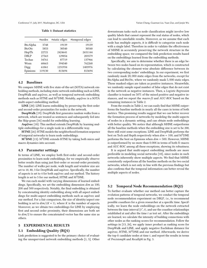
tems(Tech). The statistics of these networks are reported in Table 1.
Conference’17, July 2017, Washington, DC, USA Yutian Chang, Guannan Liu, Yuan Zuo, and Junjie Wu
Table 1: Dataset statistics
#nodes #static edges #temporal edges
BtcAlpha 3748 19139 19139
BtcOtc 5853 30540 30540
HepTh 22721 2424641 2651144
DBLP 27563 129054 203579
Techas 34761 87719 137966
Wosn 60663 594540 762268
Digg 61061 1231934 1403976
Epinions 119130 813694 813694
4.2 BaselinesWe compare MHNE with five state-of-the-art (SOTA) network em-
beddingmethods, including static network embedding such as LINE,
DeepWalk and asp2vec, as well as temporal network embedding
methods such as HTNE and M2DNE. Notably, asp2vec is a SOTA
multi-aspect embedding method.
LINE [20]: LINE learns embedding by preserving the first-order
and second-order proximities for nodes in the network.
DeepWalk [19]: DeepWalk first generates random walks from a
network, which are treated as sentences and subsequently fed into
the Skip-gram [16] model for embedding learning.
Asp2vec [18]: This method extends DeepWalk by learning mul-
tiple embeddings for a single node in a differentiable way.
HTNE [26]: HTNEmodels the neighborhood formation sequence
of temporal networks to learn node embeddings.
M2DNE [13]: M2DNE extends HTNE by taking both micro and
macro dynamics into account.
4.3 Parameter settingsIn terms of LINE, we employ both first-order and second-order
proximities to learn node embeddings, for we empirically observe
better results than using just first-order or second-order proximity.
The number of walks per node, walk length and window size are
set to 10, 80, 3 for DeepWalk and asp2vec. Specifically, the number
of aspects is set to 4 for both asp2vec and our method. The history
length is set to 5 for our method, HTNE and M2DNE.
We run each model with varying dimensions of learned embed-
dings. Specifically, we set the embedding dimension 𝑑𝑖𝑚 as 100,200 and 500 respectively. Notably, the final embedding is obtained
by concatenating identity embedding along with all aspect embed-
dings for multi-aspect embedding methods such as asp2vec and
our method. For a fair comparison, the size of identity/aspect em-
bedding is set to 𝑑𝑖𝑚/(𝐾 + 1), where 𝐾 is the number of aspects.
Moreover, as we obtain two embeddings for LINE by employing
first and second order proximity, their dimensions are both set
to 𝑑𝑖𝑚/2 to ensure the concatenated vector has the same size as
others.
5 EXPERIMENTAL RESULTS5.1 Embedding Quality (RQ1)Link prediction is suggested to be the primary choice of evaluat-
ing the unsupervised network embedding methods [1, 5]. Other
downstream tasks such as node classification might involve low
quality labels that cannot represent the real status of nodes, which
can lead to unreliable results. Moreover, as we assume that each
node has multiple aspects, it is difficult to categorize each node
with a single label. Therefore in order to validate the effectiveness
of MHNE in accurately preserving the network structure in the
embedding space, we compared the link prediction results based
on the embeddings learned from the embedding methods.
Specifically, we aim to determine whether there is an edge be-
tween two nodes based on its representation, which is constructed
by calculating the element-wise absolute difference between its
two corresponding nodes’ embeddings. In our experiment, we first
randomly mask 20, 000 static edges from the networks, except for
BtcAlpha and BtcOtc, where we randomly mask 5, 000 static edges.
Those masked edges are taken as positive instances. Meanwhile,
we randomly sample equal number of false edges that do not exist
in the network as negative instances. Then, a Logistic Regressionclassifier is trained on 50% of the mixed positive and negative in-
stances, and we report the macro-f1 and AUC-ROC based on the
remaining instances in Table 2.
From the results in Table 2, we can easily find that MHNE outper-
forms the baseline methods in nearly all the cases in terms of both
metrics. This promising results suggest that we can better recover
the formation process of networks by modeling the multi-aspects
of nodes in a dynamic setting, and can obtain node embeddings
with better quality. We notice that although MHNE outperforms
all the baseline methods when the embedding size is set to be 200,
there still exist some exceptions. LINE and DeepWalk performs the
best on Tech and Hepth respectively when 𝑑𝑖𝑚 = 100, and M2DNE
performs the best on Epinions when 𝑑𝑖𝑚 = 500. However, MHNE
is outperformed by no more than 0.006 in terms of both f1-macro
and AUC-ROC among all these exceptions, showing its robustness.
It is argued that multi-aspect embedding methods are more
preferable in modeling social networks [18], since nodes in such
networks inherently show multiple aspects. We find that MHNE
consistently outperforms all the baseline methods on the two social
networks, which is not only in line with the previous findings but
also confirms that the temporal information can better reveal the
multiple aspects of nodes.
5.2 Temporal Node Recommendation (RQ2)To further evaluate whether our method can better capture the
evolution patterns of temporal networks, we conduct the temporal
node recommendation experiment on DBLP, i.e., to recommend
possible coauthors for a given researcher at a specific time. Specif-
ically, we learn the node embeddings on the network extracted
between the time interval [𝑡 ′, 𝑡), and use the coauthor relationshipsestablished at and after the time 𝑡 as test set. After the embeddings
are learned, we calculate the intensity of building connections with
other nodes as the ranking scores for recommendation. Follow the
settings in [13, 26], we apply inner product as ranking score for
DeepWalk and LINE, and apply negative Euclidean distance for
asp2vec, HTNE, M2DNE and our method. Afterwards, we derive
the top-𝑘 candidate nodes at time 𝑡 , and report the results in terms
of Precision@k and Recall@k in Fig. 3.

Multi-Aspect Temporal Network Embedding:A Mixture of Hawkes Process View Conference’17, July 2017, Washington, DC, USA
Table 2: Link Prediction Results
Dataset dim
f1-macro AUC-ROC
LINE asp2vec DeepWalk HTNE M2DNE MHNE LINE asp2vec DeepWalk HTNE M
2DNE MHNE
DBLP
100
0.7751 0.9389 0.9073 0.9335 0.9443 0.9594 0.8459 0.9799 0.9666 0.9807 0.9851 0.9886Wosn 0.8168 0.8991 0.8896 0.9005 0.9136 0.9323 0.8889 0.9593 0.9526 0.9620 0.9691 0.9774Digg 0.8034 0.8647 0.8862 0.8444 0.8701 0.8871 0.8710 0.9348 0.9507 0.9026 0.9404 0.9522Epinions 0.7941 0.9114 0.9228 0.8916 0.9239 0.9266 0.8590 0.9649 0.9686 0.9580 0.9745 0.9749Tech 0.9172 0.8882 0.7919 0.8919 0.9043 0.9086 0.9685 0.9511 0.8709 0.9534 0.9622 0.9630
HepTh 0.8602 0.7981 0.9277 0.8556 0.8946 0.9222 0.9299 0.8776 0.9792 0.9307 0.9569 0.9737
BtcAlpha 0.8127 0.8919 0.8801 0.8834 0.9093 0.9210 0.8838 0.9514 0.9420 0.9453 0.9646 0.9712BtcOtc 0.8194 0.8954 0.8782 0.8859 0.9177 0.9285 0.8897 0.9557 0.9380 0.9465 0.9709 0.9731DBLP
200
0.8229 0.949 0.9316 0.9298 0.9426 0.9627 0.8983 0.9830 0.9765 0.9791 0.984 0.9898Wosn 0.8204 0.9147 0.8840 0.9016 0.9116 0.9311 0.8946 0.9690 0.9459 0.9623 0.9685 0.9770Digg 0.8428 0.8737 0.8808 0.8420 0.8707 0.8852 0.9076 0.9409 0.9469 0.9184 0.9404 0.9516Epinions 0.8760 0.9123 0.9199 0.8882 0.9209 0.9223 0.9346 0.9645 0.9676 0.9534 0.9724 0.9730Tech 0.9105 0.8917 0.7994 0.8865 0.9018 0.9137 0.9627 0.9527 0.8766 0.9504 0.9614 0.9670HepTh 0.8413 0.8563 0.9174 0.8529 0.8954 0.9224 0.9169 0.9278 0.9735 0.9299 0.9582 0.9737BtcAlpha 0.8492 0.9092 0.8792 0.8763 0.9069 0.9256 0.9244 0.9647 0.9394 0.9414 0.9614 0.9734BtcOtc 0.8507 0.9112 0.8790 0.8756 0.9134 0.9321 0.9231 0.9689 0.9385 0.9400 0.9681 0.9743DBLP
500
0.8228 0.9406 0.9423 0.9250 0.9383 0.9611 0.8986 0.9782 0.9798 0.9765 0.9823 0.9892Wosn 0.8037 0.9045 0.8636 0.8974 0.9115 0.9215 0.8784 0.9607 0.9305 0.9599 0.9690 0.9728Digg 0.8507 0.8778 0.8690 0.8325 0.8636 0.8795 0.9129 0.9445 0.9379 0.9110 0.9347 0.9465Epinions 0.8800 0.8894 0.9140 0.8802 0.9180 0.9116 0.9377 0.9505 0.9632 0.9499 0.9714 0.9677
Tech 0.9085 0.9030 0.8141 0.8810 0.8969 0.9115 0.9627 0.9615 0.8900 0.9474 0.9595 0.9671HepTh 0.8479 0.8650 0.9040 0.8530 0.8965 0.9156 0.9251 0.9334 0.9652 0.9283 0.9585 0.9710BtcAlpha 0.8243 0.9041 0.8758 0.8644 0.8996 0.9249 0.9032 0.9610 0.9392 0.9326 0.9576 0.9725BtcOtc 0.8123 0.9190 0.8751 0.8625 0.9052 0.9289 0.8916 0.9714 0.9399 0.9300 0.9593 0.9741
5 10 15 20k
0.10
0.15
0.20
0.25
0.30
Prec
ision
@k
LINEDeepWalkasp2vecHTNEM2DNEMHNE
(a) precision@k
5 10 15 20k
0.30
0.35
0.40
0.45
0.50
Reca
ll@k
(b) recall@k
Figure 3: Temporal Node Recommendation Results
We can find from Fig. 3 that our method consistently outper-
forms the other methods in terms of both metrics. Interestingly, we
find the three methods (MHNE, M2DNE, HTNE) which model the
formation process outperform the other static embedding methods.
This demonstrates that by modeling the dynamic neighborhood for-
mation process, the future events can be predicted more accurately.
Moreover, though asp2vec cannot compete with the temporal net-
work embedding methods, it achieve the best performances among
all the static embeddingmethods, which again provides evidence for
the necessity in considering the multiple aspects. Therefore, it also
emphasizes that multi-aspect embedding and temporal network
embedding are two tasks complement each other.
5.3 Aspect Embedding Analysis (RQ3)In this experiment, we aim to explore whether our method can
capture different aspects of nodes from the two perspectives. 1)
DBLP
Wos
nDi
ggEp
inio
nsTe
chHe
pTh
BtcA
lpha
BtcO
tc
0.5
0.6
0.7
0.8
0.9
1.0
f1-m
acro
aspect 0aspect 1
aspect 2aspect 3
identityconcat
(a) MHNE
DBLP
Wos
nDi
ggEp
inio
nsTe
chHe
pTh
BtcA
lpha
BtcO
tc
0.5
0.6
0.7
0.8
0.9
1.0
f1-m
acro
part 0part 1
part 2part 3
part 4concat
(b) HTNEFigure 4: Link Prediction with Aspect embeddings
What are the quality of the learned aspect embeddings? 2) CanMHNE capture the diverse aspect driven neighborhood formations?
5.3.1 Aspect Embedding Quality. To evaluate the quality of the
aspect embeddings, we perform the link prediction using only em-
beddings from certain aspect or identity embeddings and report
the macro-f1 in Fig. 4. For comparison, we conduct this experiment
on HTNE by splitting its node embeddings into multiple parts that
have equal size with the aspect embeddings.
Fig. 4a shows that aspect embeddings are significantly outper-
formed by the concatenated vectors consisting of both aspect em-
beddings and identity embeddings. Conversely, the performance
gap between the embeddings learned from HTNE and their splitted
parts is much smaller as illustrated in Figure. 4b. Such contrastive
results may be due to the fact that the aspect embeddings obtained
by MHNE are one-sided and cannot adequately describe the nature

Conference’17, July 2017, Washington, DC, USA Yutian Chang, Guannan Liu, Yuan Zuo, and Junjie Wu
0 5 10 15 20 25 30 35N(s)
0.230.240.250.260.27
k v|u
aspect 0 aspect 1 aspect 2 aspect 3
(a) Bolin Ding
0 5 10 15 20 25N(s)
0.22
0.24
0.26
0.28
k v|u
(b) Christopher Ré
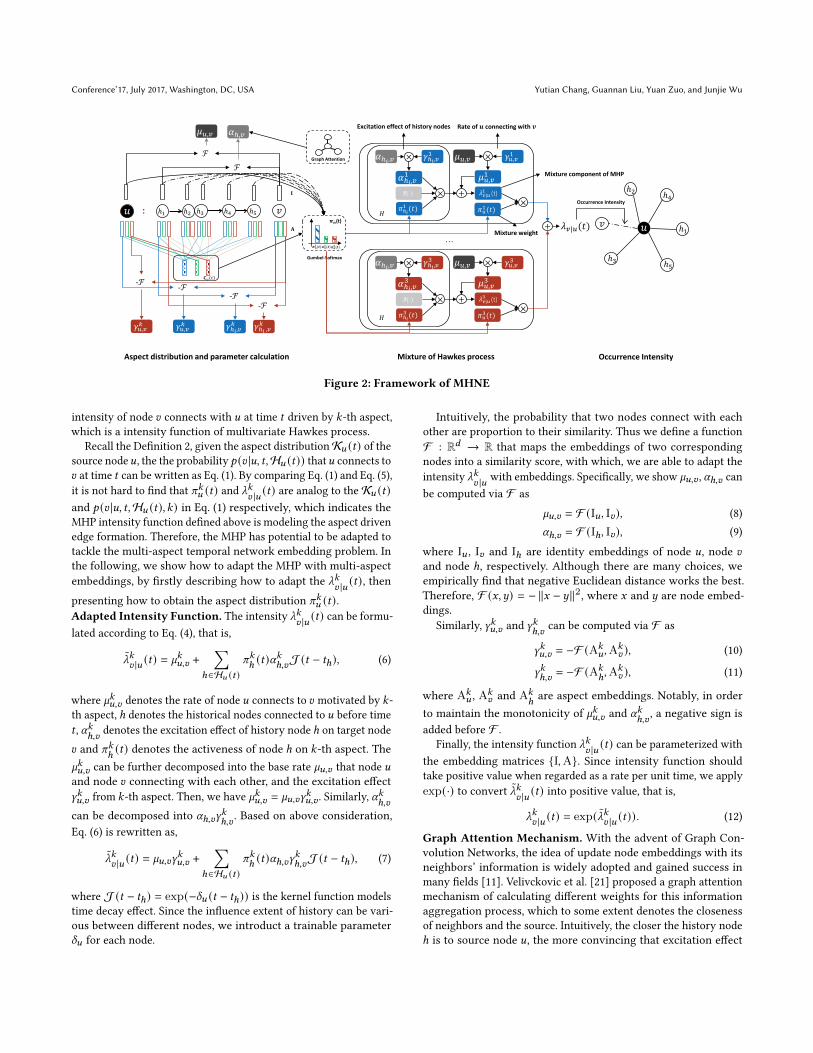
Figure 5: Aspect-driven Temporal Events
of nodes from a macro perspective, since we force each aspect em-
bedding to focus on a certain aspect. Therefore, the performance
improvement of concatenating the aspect and identity embeddings
is dramatically larger, which demonstrates that we can obtain a
more comprehensive description of nodes from its various aspects.
5.3.2 Analysis of Aspect-driven Temporal Events. In order to gain
insights on how the learned multiple different aspects affect the
occurrence of temporal events, we visualize the intensity excited
by aspect 𝑘 , i.e., _𝑘𝑣 |𝑢 of the neighborhood sequence. For illustrative
purpose, we choose two scholars, Bolin Ding and Christopher Réfrom DBLP who were previously focusing on the Database fieldand then shift the research interests to Data Mining and ArtificialIntelligence respectively. This means that Bolin Ding and ChristopherRé might collaborate with other researchers focusing on Databasein the earlier years, while their academic partnership may change
accordingly over time.
As illustrated in Fig. 5, the red lines in both subfigures repre-
senting the intensity from aspect #1 has a clear downward trend,
while the blue line in Fig. 5a and purple line in Fig. 5b keep rising
over time. This indicates that the temporal events of Bolin Ding andChristopher Ré are mostly driven by aspect#1 at the early stages.
After that, the occurrence of temporal events are primarily inspired
by aspect #0 and aspect #3 for them. Compared with previous
analysis, we infer that aspect#1 mainly represents Database forthese two authors, and aspect#0 and aspect#3 might represent
Data Mining and Artificial Intelligence respectively. These two casesdemonstrate that MHNE can capture different driving aspects for
the temporal events and can be reflected from the dynamic node
status.
5.4 Ablation Study (RQ4)To validate the effectiveness of incorporating graph attention mech-
anism and Gumbel-Softmax into our model, we construct several
submodels that deliberately removes one component or both and
test the performances of these model variants. Specifically, we
conduct link prediction with these constructed models and report
results in terms of the macro-f1 in Fig. 6.
DBLP Wosn Digg Epinions Tech HepTh BtcAlpha BtcOtc0.85
0.88
0.91
0.94
0.97
1.00
f1-m
acro
MHNEMHNE-w/o-attn
MHNE-w/o-GumbelMHNE-w/o-attn-Gumbel
Figure 6: Ablation Study
From the results we can find MHNE outperforms all the submod-
els in all the datasets, which demonstrate the rationality of incor-
porating both graph attention mechanism and Gumbel-Softmax.
Among the submodels,MHNE-w/o-attn performs the best onHepTh
and MHNE-w/o-Gumbel performs the best on Digg, BtcAlpha and
BtcOtc. In the other datasets, MHNE-w/o-attn and MHNE-w/o-
Gumbel performs on par with each other. These results verify that
MHNE benefits from graph attention mechanism by better captur-
ing the relationship between the source node and history nodes.
Moreover, Gumbel-Softmax trick enables MHNE to assign different
forms of aspect distributions for different nodes, which also im-
proves model performance. In addition, MHNE-w/o-attn-Gumbel
performs the worst in most cases.
5.5 Parameter Sensitivity (RQ5)For point process based embeddingmodels [13, 26] andmulti-aspect
embedding methods [5, 12, 18], the most important parameters are
the history length 𝐻 and the number of aspects 𝐾 respectively.
In this section, we study the sensitivity of our model by conduct-
ing link prediction experiments under different setting of the two
parameters, and we report the macro-f1 in Table 3 and Table 4.
Notably, we fix the dimension of concatenated vectors to 200, thusthe size of each aspect is set to 200/(𝐾 + 1).
As shown in Table 3, the optimal history length varies in differ-
ent datasets. While the performance has never be the best when
𝐻 = 1, we argue that MHNE benefits for a comparatively longer
history lengthwhich incorporates more information from the neigh-
borhood sequence. As illustrated in Table 4, we can see that the
macro-f1 of MHNE increases along with𝐾 and remains stable when
𝐾 >= 2. Specifically, we preserve only one aspect embedding for
each node when𝐾 = 1, which means that the multi-aspect nature is
ignored. Interestingly, MHNE performs the best when 𝐾 is set to be
the largest on the two social networks, which is in accordance with
previous discussion that the nodes in social networks inherently
exhibits multiple aspects than other networks. This result again
supports that our model can benefit from learning multiple aspect
embeddings while is robust on different number of aspects across
all the datasets.
6 RELATEDWORKNetwork embedding methods represent each node in the network
via low-dimensional vectors while preserving network structure,
have gained wide attention in recent years [2], and our work is
related to the following categories of studies.

Multi-Aspect Temporal Network Embedding:A Mixture of Hawkes Process View Conference’17, July 2017, Washington, DC, USA
Table 3: Link prediction over different history length
𝐻 1 2 3 4 5
DBLP 0.9613 0.9613 0.9603 0.9596 0.9599
Wosn 0.9276 0.9289 0.9300 0.9290 0.9286
Digg 0.8885 0.8872 0.8878 0.8882 0.8892Epinions 0.9228 0.9243 0.9247 0.9261 0.9262Tech 0.9119 0.9128 0.9143 0.9129 0.9119
HepTh 0.9273 0.9287 0.9294 0.9288 0.9232
BtcAlpha 0.9283 0.9302 0.9310 0.9293 0.9296
BtcOtc 0.9378 0.9367 0.9349 0.9393 0.9346
Table 4: Link prediction over different number of aspects
𝐾 1 3 4 7 9
DBLP 0.9579 0.9622 0.9624 0.9615 0.9601
Wosn 0.9186 0.9283 0.9295 0.9312 0.9315Digg 0.8608 0.8851 0.8825 0.8912 0.8923Epinions 0.8966 0.9165 0.9194 0.9252 0.9249
Tech 0.9024 0.9089 0.9099 0.9080 0.9086
HepTh 0.8757 0.9177 0.9230 0.9240 0.9299BtcAlpha 0.9106 0.9260 0.9230 0.9262 0.9234
BtcOtc 0.9184 0.9294 0.9290 0.9292 0.9324
Network embedding.Mikolov et al. [15, 16] proposes an effi-
cient embedding learning method for words and phrases in natu-
ral language. Inspired by their work, several random walk based
network embedding methods are developed by making analogy
between nodes and words in natural language. For example, Deep-
Walk [19] and node2vec [7] use truncated random walks generated
from a network as the input of skip-gram model to learn node em-
beddings. Besides, LINE [20] optimizes node embeddings by preserv-
ing first-order and second-order proximities in both vertex and em-
bedding space. Graph Convolutional Networks(GCNs) are another
approach on representation learning based on the message-passing-
receiving mechanism, which is to update a node’s representation
by aggregating information from its neighbors [8, 10, 21]. However,
most GCNs are supervised or semi-supervised method thus has a
strong requirement for a large amount of labeled data [11].
Temporal network embedding. These aforementioned meth-
ods all focus on static networks, however, in reality, the majority
of networks evolve over time. [4, 17] adapt conventional GCNs to
model temporal networks by modeling multiple snapshots derived
from different time windows. [6] employs deep autoencoders on
derived network snapshots, and the structure of the autoencoder
evolves along with the growing of network scale. In contrast to the
snapshot based methods, some efforts [13, 26] view the formation
of temporal networks as adding nodes and edges and they trace
back the formation process by tracking the neighborhood forma-
tion of each node. For example, zuo et al. [26] proposes HTNE by
modeling the neighborhood formation sequence with a multivari-
ate Hawkes process. M2DNE [13] extends HTNE by incorporating
both micro and macro dynamics of the network, namely neighbor-
hood formation and network scale. Mei et al. [14] proposed Neural
Hakes process by using a continuous LSTM model to better reveal
the sophisticated mutual effect between history and future events.
However, the underlying mechanism of how temporal edges are
formed driven by different aspect is ignored in prior work, which
is crucial to model the multi-aspect temporal networks.
Multi-aspect embedding. There exists some recent research [5,
12, 18, 22] learning multiple embedding vectors for each node in
order to capture the multifaceted nature of nodes. Liu et al. [12]
proposes PolyDW by extending DeepWalk to multi-aspect embed-
ding setting, it determines the aspect distribution for each node via
matrix factorization before embedding learning. Then the activated
aspect of both target node and context node is sampled from the
computed distribution, respectively. Splitter [5] firstly creates a per-
sona graph from the original network via a cluster algorithm that
maps each node to one or multiple personas, on which a random
walk based embedding method is performed to learn embeddings
for each persona. Therefore it can obtain one or multiple repre-
sentations for each node. However it blindly trains each persona
to be close to the representation of its original node and cannot
be trained in an end-to-end fashion. MCNE [22] is a GCN based
method that utilizes binary mask layers to create multiple condi-
tional embeddings for each node. MCNE is a supervised method and
requires predefined aspects(ie. different user behaviors). MNE [23]
uses matrix factorization to obtain multiple embeddings for each
node and considers the diversity of learned multiple embeddings.
However, it ignores that the aspect of each node is dependent to its
local structure. Park et al. [18] proposes Asp2vec that determines
the activated aspect of source node based on its context in current
random walks. While the truncated walks cannot fully recover
the neighborhood structure of nodes thus may provide a biased
evidence on inferring node aspects, it is more desirable to model
the multiple aspect of nodes via the detailed formation process of
nodes.
7 CONCLUSIONIn this paper, we present a novel multi-aspect embedding method
called MHNE that models the aspect driven edge formation process
of temporal networks via Mixture of Hawkes process. Moreover,
we utilize Gumbel-Softmax with trainable temperature parameter
to compute aspect distributions with different shapes. To better
capture the closeness between source and history target nodes,
graph attention mechanism is incorporated to assign larger weights
for more convincing excitation effects. Experiments on eight real-
world datasets demonstrate the effectiveness of MHNE.
REFERENCES[1] Sami Abu-El-Haija, Bryan Perozzi, and Rami Al-Rfou. 2017. Learning edge
representations via low-rank asymmetric projections. In Proceedings of CIKM.
1787–1796.
[2] Peng Cui, Xiao Wang, Jian Pei, and Wenwu Zhu. 2018. A survey on network
embedding. IEEE TKDE 31, 5 (2018), 833–852.
[3] Quanyu Dai, Qiang Li, Jian Tang, and Dan Wang. 2018. Adversarial network
embedding. In Proceedings of AAAI, Vol. 32.[4] Songgaojun Deng, Huzefa Rangwala, and Yue Ning. 2019. Learning Dynamic
Context Graphs for Predicting Social Events. In Proceedings of SIGKDD. 1007–1016.
[5] Alessandro Epasto and Bryan Perozzi. 2019. Is a single embedding enough?
learning node representations that capture multiple social contexts. InWWW.
394–404.
[6] Palash Goyal, Nitin Kamra, Xinran He, and Yan Liu. 2018. Dyngem: Deep em-
bedding method for dynamic graphs. arXiv preprint arXiv:1805.11273 (2018).[7] Aditya Grover and Jure Leskovec. 2016. node2vec: Scalable feature learning for
networks. In Proceedings of SIGKDD. 855–864.
Conference’17, July 2017, Washington, DC, USA Yutian Chang, Guannan Liu, Yuan Zuo, and Junjie Wu
[8] Will Hamilton, Zhitao Ying, and Jure Leskovec. 2017. Inductive representation
learning on large graphs. In NeurIPS. 1024–1034.[9] Eric Jang, Shixiang Gu, and Ben Poole. 2016. Categorical reparameterization
with gumbel-softmax. arXiv preprint arXiv:1611.01144 (2016).[10] Thomas N Kipf and MaxWelling. 2016. Semi-supervised classification with graph
convolutional networks. arXiv preprint arXiv:1609.02907 (2016).
[11] Qimai Li, Zhichao Han, and Xiao-Ming Wu. 2018. Deeper insights into graph
convolutional networks for semi-supervised learning. In Proceedings of AAAI,Vol. 32.
[12] Ninghao Liu, Qiaoyu Tan, Yuening Li, Hongxia Yang, Jingren Zhou, and Xia
Hu. 2019. Is a single vector enough? exploring node polysemy for network
embedding. In Proceedings of SIGKDD. 932–940.[13] Yuanfu Lu, Xiao Wang, Chuan Shi, Philip S Yu, and Yanfang Ye. 2019. Temporal
network embedding with micro-and macro-dynamics. In Proceedings of CIKM.
469–478.
[14] Hongyuan Mei and Jason Eisner. 2017. The Neural Hawkes Process: A Neurally
Self-Modulating Multivariate Point Process. In NeuraIPS.[15] Tomas Mikolov, Kai Chen, Greg Corrado, and Jeffrey Dean. 2013. Efficient
estimation of word representations in vector space. arXiv preprint arXiv:1301.3781(2013).
[16] Tomas Mikolov, Ilya Sutskever, Kai Chen, Greg S Corrado, and Jeff Dean. 2013.
Distributed representations of words and phrases and their compositionality. InNeurIPS 26 (2013), 3111–3119.
[17] Aldo Pareja, Giacomo Domeniconi, Jie Chen, Tengfei Ma, Toyotaro Suzumura,
Hiroki Kanezashi, Tim Kaler, Tao B Schardl, and Charles E Leiserson. 2020.
EvolveGCN: Evolving Graph Convolutional Networks for Dynamic Graphs. In
AAAI. 5363–5370.[18] Chanyoung Park, Carl Yang, Qi Zhu, Donghyun Kim, Hwanjo Yu, and Jiawei
Han. 2020. Unsupervised Differentiable Multi-aspect Network Embedding. arXivpreprint arXiv:2006.04239 (2020).
[19] Bryan Perozzi, Rami Al-Rfou, and Steven Skiena. 2014. Deepwalk: Online learning
of social representations. In Proceedings of SIGKDD. 701–710.[20] Jian Tang, Meng Qu, Mingzhe Wang, Ming Zhang, Jun Yan, and Qiaozhu Mei.
2015. Line: Large-scale information network embedding. In Proceedings of WWW.
1067–1077.
[21] Petar Veličković, Guillem Cucurull, Arantxa Casanova, Adriana Romero, Pietro
Lio, and Yoshua Bengio. 2017. Graph attention networks. arXiv preprintarXiv:1710.10903 (2017).
[22] Hao Wang, Tong Xu, Qi Liu, Defu Lian, Enhong Chen, Dongfang Du, Han Wu,
and Wen Su. 2019. MCNE: An end-to-end framework for learning multiple
conditional network representations of social network. In Proceedings of SIGKDD.1064–1072.
[23] Liang Yang, Yuanfang Guo, and Xiaochun Cao. 2018. Multi-facet network embed-
ding: Beyond the general solution of detection and representation. In Proceedingsof AAAI, Vol. 32.
[24] Shuang-Hong Yang and Hongyuan Zha. 2013. Mixture of mutually exciting
processes for viral diffusion. In ICML. 1–9.[25] Lekui Zhou, Yang Yang, Xiang Ren, Fei Wu, and Yueting Zhuang. 2018. Dynamic
network embedding by modeling triadic closure process. In Proceedings of AAAI,Vol. 32.
[26] Yuan Zuo, Guannan Liu, Hao Lin, Jia Guo, Xiaoqian Hu, and Junjie Wu. 2018.
Embedding temporal network via neighborhood formation. In Proceedings ofSIGKDD. 2857–2866.
Multi-Aspect Temporal Network Embedding:A Mixture of Hawkes Process View Conference’17, July 2017, Washington, DC, USA
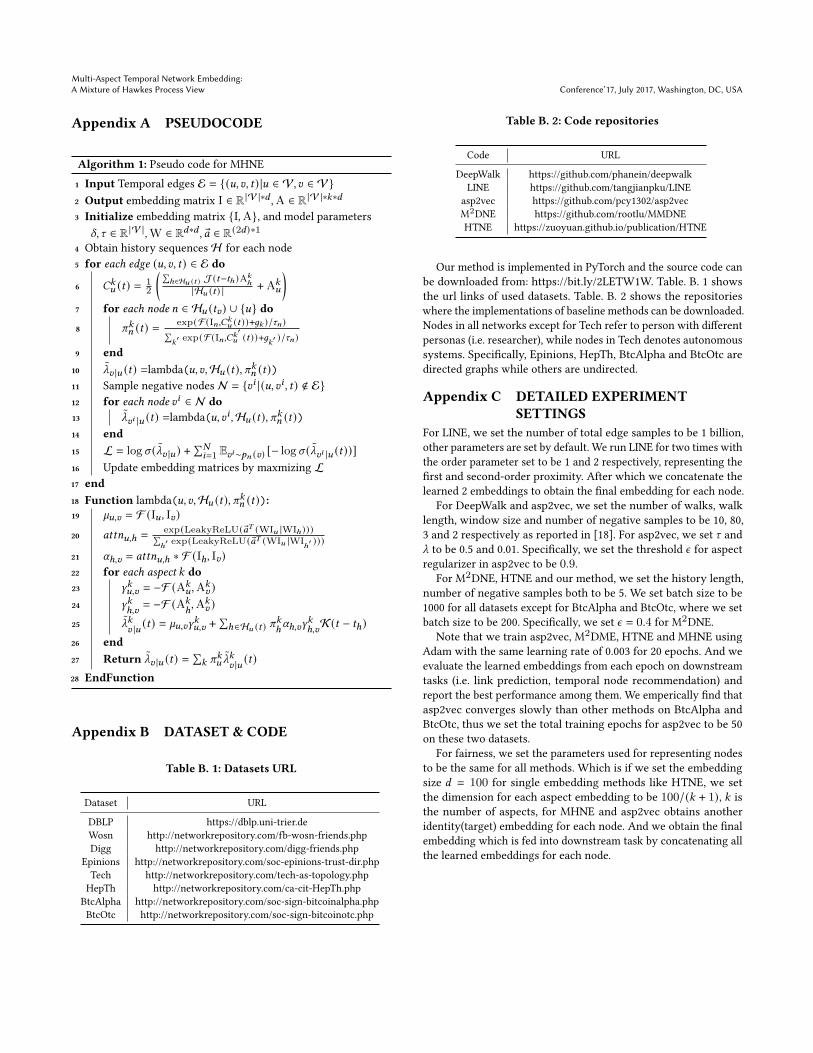
Appendix A PSEUDOCODE
Algorithm 1: Pseudo code for MHNE
1 Input Temporal edges E = {(𝑢, 𝑣, 𝑡) |𝑢 ∈ V, 𝑣 ∈ V}2 Output embedding matrix I ∈ R |V |∗𝑑 ,A ∈ R |V |∗𝑘∗𝑑
3 Initialize embedding matrix {I,A}, and model parameters
𝛿, 𝜏 ∈ R |V |,W ∈ R𝑑∗𝑑 , ®𝑎 ∈ R(2𝑑)∗14 Obtain history sequencesH for each node
5 for each edge (𝑢, 𝑣, 𝑡) ∈ E do
6 𝐶𝑘𝑢 (𝑡) = 12
(∑ℎ∈H𝑢 (𝑡 ) J(𝑡−𝑡ℎ)A𝑘
ℎ
|H𝑢 (𝑡 ) | +A𝑘𝑢
)7 for each node 𝑛 ∈ H𝑢 (𝑡𝑣) ∪ {𝑢} do8 𝜋𝑘𝑛 (𝑡) =
exp(F(I𝑛,𝐶𝑘𝑢 (𝑡 ))+𝑔𝑘 )/𝜏𝑛)∑
𝑘′ exp(F(I𝑛,𝐶𝑘
′𝑢 (𝑡 ))+𝑔
𝑘′ )/𝜏𝑛)
9 end10 _̃𝑣 |𝑢 (𝑡) =lambda(𝑢, 𝑣,H𝑢 (𝑡), 𝜋𝑘𝑛 (𝑡))11 Sample negative nodes N = {𝑣𝑖 | (𝑢, 𝑣𝑖 , 𝑡) ∉ E}12 for each node 𝑣𝑖 ∈ N do13 _̃𝑣𝑖 |𝑢 (𝑡) =lambda(𝑢, 𝑣𝑖 ,H𝑢 (𝑡), 𝜋𝑘𝑛 (𝑡))14 end15 L = log𝜎 (_̃𝑣 |𝑢 ) +
∑𝑁𝑖=1 E𝑣𝑖∼𝑝𝑛 (𝑣) [− log𝜎 (_̃𝑣𝑖 |𝑢 (𝑡))]
16 Update embedding matrices by maxmizing L17 end18 Function lambda(𝑢, 𝑣,H𝑢 (𝑡), 𝜋𝑘𝑛 (𝑡)):19 `𝑢,𝑣 = F (I𝑢 , I𝑣)20 𝑎𝑡𝑡𝑛𝑢,ℎ =
exp(LeakyReLU( ®𝑎𝑇 (WI𝑢 |WIℎ)))∑ℎ′ exp(LeakyReLU( ®𝑎𝑇 (WI𝑢 |WI
ℎ′ )))
21 𝛼ℎ,𝑣 = 𝑎𝑡𝑡𝑛𝑢,ℎ ∗ F (Iℎ, I𝑣)22 for each aspect 𝑘 do23 𝛾𝑘𝑢,𝑣 = −F (A𝑘𝑢 ,A𝑘𝑣 )24 𝛾𝑘
ℎ,𝑣= −F (A𝑘
ℎ,A𝑘𝑣 )
25 _̃𝑘𝑣 |𝑢 (𝑡) = `𝑢,𝑣𝛾
𝑘𝑢,𝑣 +
∑ℎ∈H𝑢 (𝑡 ) 𝜋
𝑘ℎ𝛼ℎ,𝑣𝛾
𝑘ℎ,𝑣
K(𝑡 − 𝑡ℎ)26 end27 Return _̃𝑣 |𝑢 (𝑡) =
∑𝑘 𝜋
𝑘𝑢 _̃
𝑘𝑣 |𝑢 (𝑡)
28 EndFunction
Appendix B DATASET & CODE
Table B. 1: Datasets URL
Dataset URL
DBLP https://dblp.uni-trier.de
Wosn http://networkrepository.com/fb-wosn-friends.php
Digg http://networkrepository.com/digg-friends.php
Epinions http://networkrepository.com/soc-epinions-trust-dir.php
Tech http://networkrepository.com/tech-as-topology.php
HepTh http://networkrepository.com/ca-cit-HepTh.php
BtcAlpha http://networkrepository.com/soc-sign-bitcoinalpha.php
BtcOtc http://networkrepository.com/soc-sign-bitcoinotc.php
Table B. 2: Code repositories
Code URL
DeepWalk https://github.com/phanein/deepwalk
LINE https://github.com/tangjianpku/LINE
asp2vec https://github.com/pcy1302/asp2vec
M2DNE https://github.com/rootlu/MMDNE
HTNE https://zuoyuan.github.io/publication/HTNE
Our method is implemented in PyTorch and the source code can
be downloaded from: https://bit.ly/2LETW1W. Table. B. 1 shows
the url links of used datasets. Table. B. 2 shows the repositories
where the implementations of baseline methods can be downloaded.
Nodes in all networks except for Tech refer to person with different
personas (i.e. researcher), while nodes in Tech denotes autonomous
systems. Specifically, Epinions, HepTh, BtcAlpha and BtcOtc are
directed graphs while others are undirected.
Appendix C DETAILED EXPERIMENTSETTINGS
For LINE, we set the number of total edge samples to be 1 billion,
other parameters are set by default. We run LINE for two times with
the order parameter set to be 1 and 2 respectively, representing the
first and second-order proximity. After which we concatenate the
learned 2 embeddings to obtain the final embedding for each node.
For DeepWalk and asp2vec, we set the number of walks, walk
length, window size and number of negative samples to be 10, 80,
3 and 2 respectively as reported in [18]. For asp2vec, we set 𝜏 and
_ to be 0.5 and 0.01. Specifically, we set the threshold 𝜖 for aspect
regularizer in asp2vec to be 0.9.For M
2DNE, HTNE and our method, we set the history length,
number of negative samples both to be 5. We set batch size to be
1000 for all datasets except for BtcAlpha and BtcOtc, where we set
batch size to be 200. Specifically, we set 𝜖 = 0.4 for M2DNE.
Note that we train asp2vec, M2DME, HTNE and MHNE using
Adam with the same learning rate of 0.003 for 20 epochs. And we
evaluate the learned embeddings from each epoch on downstream
tasks (i.e. link prediction, temporal node recommendation) and
report the best performance among them. We emperically find that
asp2vec converges slowly than other methods on BtcAlpha and
BtcOtc, thus we set the total training epochs for asp2vec to be 50
on these two datasets.
For fairness, we set the parameters used for representing nodes
to be the same for all methods. Which is if we set the embedding
size 𝑑 = 100 for single embedding methods like HTNE, we set
the dimension for each aspect embedding to be 100/(𝑘 + 1), 𝑘 is
the number of aspects, for MHNE and asp2vec obtains another
identity(target) embedding for each node. And we obtain the final
embedding which is fed into downstream task by concatenating all
the learned embeddings for each node.