Embed Size (px)
Citation preview
Research in Astron. Astrophys. Vol.0 (20xx) No.0, 000–000
http://www.raa-journal.org http://www.iop.org/journals/raaResearch inAstronomy andAstrophysics
Multi-Aperture Seeing Profiler with Multiple Guide Stars
Feng Yang1,2,4, Gang Zhao1,2 and De-Qing Ren1,2,3
1 National Astronomical Observatories / Nanjing Institute of Astronomical Optics & Technology,
Chinese Academy of Sciences, Nanjing 210042, China; [email protected] CAS Key Laboratory of Astronomical Optics & Technology, Nanjing Institute of Astronomical
Optics & Technology, Nanjing 210042, China3 Physics & Astronomy Department, California State University Northridge, 18111 Nordhoff Street,
Northridge, California 91330-8268, USA4 University of Chinese Academy of Sciences, Beijing 100049, China
Received 2018 July 13; accepted 2018 October 24
Abstract Day-time atmospheric turbulence profile is crucial for the design of both optical
system and control algorithm of solar Multi-Conjugate Adaptive Optics (MCAO) system.
Multi-Aperture Seeing Profiler (MASP) is a portable instrument which can measure the
day-time turbulence profile up to ∼ 30 km. It consists of two portable small telescopes
and could have similar performance as a Solar-Differential Image Motion Monitor + (S-
DIMM+) on a 1.0 m solar telescope. In the original design of MASP, only two guide
stars are used to retrieve the turbulence profile. In this paper, we studied the usage of
multiple guide stars in MASP using numerical simulation, and found that there are mainly
three advantages. Firstly, the precision of turbulence profile can be increased, especially
at the height about 15 km, which is important for characterizing the turbulences at the
tropopause. Secondly, the equivalent diameter of MASP can be increased up to 30%,
which will reduce the cost and weight of the instruments. Thirdly, the vertical resolution
of turbulence profile near ground increase with the help of multiple guide stars.
Key words: atmospheric effects — site testing — methods: numerical
1 INTRODUCTION
Atmosphere turbulence profile which describes the strength of turbulences at different altitudes, plays
a crucial role for the design of advanced adaptive optics (AO) systems such as Ground-Layer Adaptive
Optics (GLAO, Ren, Jolissaint et al. 2015), Multi-Conjugate Adaptive Optics (MCAO, Rimmele et al.
2010) and Tomographic Adaptive Optics (TAO, Ren et al. 2014). On one hand, turbulence profile is
important in the optical design and optimization of the AO systems. In MCAO system, the deformable
mirros (DMs) are located at the conjugated heights of turbulence layers, thus the number and conjugated
heights of DMs rely on the distribution and strength of turbulences. On the other hand, turbulence
profile is also important in the optimization of the control algorithm of AO system. For example, prior
information of turbulence profile is necessary to optimize the FOV of MCAO (Tokovinin et al. 2000).
Solar MCAO is crucial for solar observation, since the field-of-view (FOV) of conventional solar AO
is only about 10′′ (Beckers 1988; Rimmele & Radick 1998) and is too small for the observation of the
solar activity region which is as large as 1 - 2′. In the design of the solar MCAO, the day time turbulence
profile is critical. In the future, large solar telescope such as Daniel K. Inouye Solar Telescope (DKIST,

2 F. Yang, G. Zhao & D. Q. Ren
Elmore et al. 2014), and European Solar Telescope(EST, Collados et al. 2010) will be equipped with
MCAO systems, thus the measurement of daytime turbulence profile of these sites is important.
There are several methods to measure the turbulence profile. They are mainly divided into
scintillation-based methods and slope-based methods. The scintillation-based methods such as Multi-
Aperture Scintillation Sensors (MASS, Tokovinin et al. 2003) and SCIntillation Detection and Ranging
(SCIDAR, Vernin & Munoz-Tunon 1994; Egner & Masciadri 2007; Avila et al. 2008) are often used
in night-time seeing profile measurements. For daytime measurement, Scintillation-based methods are
only suitable to obtain the seeing profile near ground. Beckers (2001) proposed the SHadow BAnd
Ranger (SHABAR) instrument, which measured the scintillations of the whole solar disk and can only
detected the seeing profile with a maximum height of ∼ 500m. Slope-based methods include such as
SLOpe Detection And Ranging (SLODAR, Wilson 2002; Butterley et al. 2006) and Solar-Differential
Image Motion Monitor + (S-DIMM+, Scharmer & van Werkhoven 2010). S-DIMM+ which can de-
tected the turbulence profile up to 30 km is widely used in day-time turbulence profile measurements.
It has been successfully applied to obtain the seeing profile with the 1.6-meter New Solar Telescopes
at the Big Bear Solar Observatory (Kellerer et al. 2012) and the 1-meter Swedish Solar Telescope at
La Palma (Townson et al. 2014). Using the turbulence profile of BBSO which detected by S-DIMM+,
Kellerer et al. (2012) suggested the conjugated heights of the two DMs in BBSO MCAO system to be
0 km and 3 km, and the isoplanatic angle could exceeds 100′′ after AO corrections.
In S-DIMM+, the turbulence profile is measured using a wide Field of View (FOV) solar wavefront
sensor equipped after a facility solar telescope by observing the granule structure of the solar surface.
Subsections on the image of each aperture are served as guide stars at different field angles. Image
displacements of the subsections are used to retrieve the turbulence profile. Since this method based on
the differential measurements of image displacements, so it is insensitive to track error and vibrations of
the telescope. Based on the principle of triangulation, the sample heights of S-DIMM+ can be expressed
as h = s/δα, where s is the distance between any two sub-apertures, and δα is angular separation of two
guide stars. Therefore, the maximum measured height of S-DIMM+ is hmax = D/δα, where D is the
diameter of the solar telescope. And the vertical resolution is δh = w/δα, where w is the size of each
sub-aperture. In order to reduce cross-correlation error, the sizes of subfields are generally larger than
5′′ (Scharmer & van Werkhoven 2010; Kellerer et al. 2012; Ren, Zhao et al. 2015). Therefore at least a
telescope with diameter of 0.6 m is necessary for S-DIMM+ to retrieve the turbulence profile as high as
30 km.
In order to overcome the disadvantage of S-DIMM+ which need large telescope, Ren, Zhao et al.
(2015) introduced the idea of Multiple-Aperture-Based Solar Seeing Profiler (MASP). The MASP con-
sists of two small telescopes thus it is portable and flexible for the site seeing test where no facility solar
telescope can be used. A wide field Shack-Hartmann wavefront sensor (SHWFS) is equipped behind
each telescope. The turbulence profile retrieving algorithm is similar as S-DIMM+ but with an extra
term to correct the relative guide errors of the two telescopes. The equivalent diameter of MASP is
about 3 times as that of the small telescopes. Using two small telescopes with diameter of 400 mm,
the MASP could achieve similar performance as a S-DIMM+ at a 1120 mm telescope, and are able to
retrieve the turbulence profile up to 30 km.
In S-DIMM+ measurement, multiple guide stars can be used to increase the precession of turbu-
lence retrieving since more independent measurements can be done. Furthermore, fewer sub-apertures
are needed to measure the turbulence profile with multiple guide stars. Waldmann et al. (2007, 2008)
proposed a method similar as S-DIMM+, but with fewer sub-apertures and many more field directions.
Ren & Zhao (2016) introduced the idea of Advanced Multiple Aperture Seeing Profiler(A-MASP). In
A-MASP, only two smaller telescopes (or two sub-apertures) with no SHWFS are used to measure the
turbulence profile up to 20 km. Using the idea of A-MASP, the turbulence profile above the site of DST
telescope at National Solar Observatory are measured by Ren et al. (2018). Multiple guide stars can
also help to increase the vertical resolution of turbulence profile. In Scharmer & van Werkhoven (2010),
multiple guide stars are used to increase the resolution of turbulence profile near ground. Wang et al.
(2018) showed that additional height grids for characterizing daytime seeing profiles can be introduced
if multiple guide stars are used.

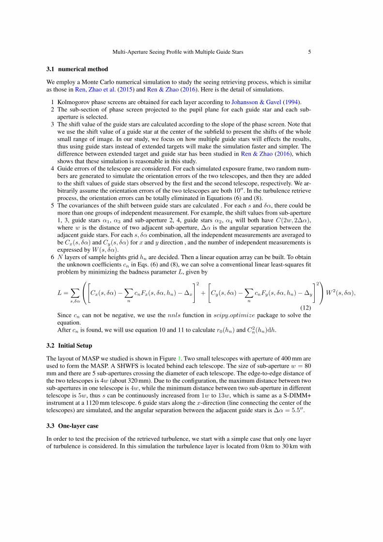
Multi-Aperture Seeing Profile with Multiple Guide Stars 3
1 3 542 10 12 141311
x
9876
y
Telescope 1 Telescope 2
w
Fig. 1 Layout of the MASP. Two circles indicate the two small telescopes. Grids in solid line
shows the layout of the SHWFS, and the grid of dashed lines indicates the gap between the
two telescopes.
In this publication, usage of multiple guide stars in MASP will be studied. If multiple guide stars
are used, the precision of turbulence profile as well as the configuration of the MASP can both be
improved. This paper is organized as follow. In Section 2, the turbulence retrieving algorithm of MASP
is described. In section 3, we compare the precession of MASP with two guide stars and multiple guide
stars using numerical simulation. In section 4, we show that the configuration of MASP can be improved
with the help of multiple guide stars. In section 5, the issue of vertical resolution of turbulence profile is
discussed. Summary is made in section 6.
2 TURBULENCE PROFILE RETRIEVING ALGORITHM OF MASP
A MASP consists of two portable small telescopes instead of a single large aperture. After each tele-
scope, a wide-field SHWFS is equipped. Figure 1 shows the layout of MASP. The two circles indicate
the apertures of the small telescopes, and the grid shows the sub-apertures of SHWFS with size of w×w.
The lenlets array of the SHWFS is along the line connecting the centers of two apertures, which is set to
be x-direction. A gap exists between the two small telescopes and is indicted by grids of dotted lines. We
mainly use the center row of the sub-apertures to retrieve the turbulence profile, and they are numbered
in the figure.
In the measurement, the same region of solar surface is observed simultaneously by the two tele-
scopes. Subfileds with size of θ×θ are selected from the image of each sub-aperture, and they served as
guide stars (Here in after we will call the subfield as guide stars for simplify). The guide stars are uni-
formly distributed along the x-direction, with ∆α between two adjacent guide stars. For the i-th guide
stars, its field angle is represented to be αi.
Using image cross-correlation, the x-component of displacement of the i-th guide star in two sub-
apertures can be measured as δx(s, αi), where s is the distance of the two sub-apertures. For the case
that the two sub-aperture are located at different telescopes, we have δx(s, αi) = δx(s, αi) + δxtel,
where δx(s, αi) is the displacement made from atmosphere turbulence, and δtel is the displacement
caused by the direction errors of telescopes. While the two sub-apertures are in the same telescope,
δx(s, αi) = δx(s, αi).When the two sub-apertures are in the same telescope, we can directly use the turbulence profile
retrieving algorithm of S-DIMM+ (Scharmer & van Werkhoven 2010). Assuming that the guide star
displacement is due to added contributions from the N turbulence layers located at heights hn, the
covariance between two guide stars can be expressed as
〈δx(s, αi)δx(s, αj)〉 =
N∑
n=1
cnFx (s, αi − αj , hn) , (1)
4 F. Yang, G. Zhao & D. Q. Ren
and
〈δy(s, αi)δy(s, αj)〉 =N∑
n=1
cnFy (s, αi − αj , hn) . (2)
where cn indicates the strength of the turbulence layers, and Fx, Fy have the following expression,
Fx(s, α, h) = I[(θh− s)/Deff , 0]/2 + I[(θh+ s)/Deff , 0]/2− I[θh/Deff , 0], (3)
Fy(s, θ, h) = I[(θh− s)/Deff , π/2]/2 + I[(θh+ s)/Deff , π/2]/2− I[θh/Deff , π/2].
I(u, 0) and I(u, π/2) are the atmospheric structure functions, and Deff = w + θhn is the effective
diameter. For the circle apertures we used, I(u, 0) and I(u, π/2) have the forms according to Kellerer
(2015)
I(u, 0) = 2− |1− u|5/3 + 2|u|5/3 − |1 + u|5/3, (4)
I(u, π/2) = 2 + 2|u|5/3 − 2(1 + u2)5/6.
When the two sub-apertures are located at different telescopes. We follow the turbulence profile
retrieving algorithm of MASP (Ren, Zhao et al. 2015). For individual exposures, the orientations of the
telescopes are fixed, and δxtel is also a fixed value for each guide star. Thus the differential value of
δx(s, αi) and δx(s, αj) will not contain the orientation error anymore.
〈[δx(s, αi)− δx(s, αj)]2〉 = 〈[δx(s, αi)− δx(s, αj)]
2〉 (5)
Expanding it, we can have
〈δx(s, αi)δx(s, αj)〉 =N∑
n=1
cnFx (s, αi − αj , hn) + ∆x. (6)
where
∆x = 〈δx2(αi)〉/2 + 〈δx2(αj)〉/2−∑
cnI(s/Deff , 0) (7)
Similar for y-direction, we have
〈δy(s, αi)δy(s, αj)〉 =
N∑
n=1
cnFy (s, αi − αj , hn) + ∆y (8)
where
∆y = 〈δy2(αi)〉/2 + 〈δy2(αj)〉/2−∑
cnI(s/Deff , π/2) (9)
Then equations array can be listed using Equations 6 and 8, and cn can be solved, which is related
to the Fried parameter r0 of the layer at hn through
cn = 0.358λ2r−5/30
(hn)D−1/3eff
(hn), (10)
where λ is the wavelength, z is the zenith angle. We can also express the results in terms of the atmo-
spheric refractive index of each layer as
C2
n(hn) = 0.16D−1/3eff
(hn) cos(z)cn. (11)
3 PRECESSION OF MASP WITH MULTIPLE GUIDE STARS
In the original design of MASP, only two guide stars are used. If we increase the number of guide stars,
for each s and δα, more independent measurement can be done. For example, if four guide stars are
used, we will have as many as 6 times more independent measurement than those of the two guide stars
case, which could increase the precision of turbulence profile measurement. In this section, we will use
numerical simulation to detailedly study the precision of MASP with multi-guide stars.
Multi-Aperture Seeing Profile with Multiple Guide Stars 5
3.1 numerical method
We employ a Monte Carlo numerical simulation to study the seeing retrieving process, which is similar
as those in Ren, Zhao et al. (2015) and Ren & Zhao (2016). Here is the detail of simulations.
1 Kolmogorov phase screens are obtained for each layer according to Johansson & Gavel (1994).
2 The sub-section of phase screen projected to the pupil plane for each guide star and each sub-
aperture is selected.
3 The shift value of the guide stars are calculated according to the slope of the phase screen. Note that
we use the shift value of a guide star at the center of the subfield to present the shifts of the whole
small range of image. In our study, we focus on how multiple guide stars will effects the results,
thus using guide stars instead of extended targets will make the simulation faster and simpler. The
difference between extended target and guide star has been studied in Ren & Zhao (2016), which
shows that these simulation is reasonable in this study.
4 Guide errors of the telescope are considered. For each simulated exposure frame, two random num-
bers are generated to simulate the orientation errors of the two telescopes, and then they are added
to the shift values of guide stars observed by the first and the second telescope, respectively. We ar-
bitrarily assume the orientation errors of the two telescopes are both 10′′. In the turbulence retrieve
process, the orientation errors can be totally eliminated in Equations (6) and (8).
5 The covariances of the shift between guide stars are calculated . For each s and δα, there could be
more than one groups of independent measurement. For example, the shift values from sub-aperture
1, 3, guide stars α1, α3 and sub-aperture 2, 4, guide stars α2, α4 will both have C(2w, 2∆α),where w is the distance of two adjacent sub-aperture, ∆α is the angular separation between the
adjacent guide stars. For each s, δα combination, all the independent measurements are averaged to
be Cx(s, δα) and Cy(s, δα) for x and y direction , and the number of independent measurements is
expressed by W (s, δα).6 N layers of sample heights grid hn are decided. Then a linear equation array can be built. To obtain
the unknown coefficients cn in Eqs. (6) and (8), we can solve a conventional linear least-squares fit
problem by minimizing the badness parameter L, given by
L =∑
s,δα
[
Cx(s, δα)−∑
n
cnFx(s, δα, hn)−∆x
]2
+
[
Cy(s, δα)−∑
n
cnFy(s, δα, hn)−∆y
]2
W 2(s, δα),
(12)
Since cn can not be negative, we use the nnls function in scipy.optimize package to solve the
equation.
After cn is found, we will use equation 10 and 11 to calculate r0(hn) and C2n(hn)dh.
3.2 Initial Setup
The layout of MASP we studied is shown in Figure 1. Two small telescopes with aperture of 400 mm are
used to form the MASP. A SHWFS is located behind each telescope. The size of sub-aperture w = 80
mm and there are 5 sub-apertures crossing the diameter of each telescope. The edge-to-edge distance of
the two telescopes is 4w (about 320 mm). Due to the configuration, the maximum distance between two
sub-apertures in one telescope is 4w, while the minimum distance between two sub-aperture in different
telescope is 5w, thus s can be continuously increased from 1w to 13w, which is same as a S-DIMM+
instrument at a 1120 mm telescope. 6 guide stars along the x-direction (line connecting the center of the
telescopes) are simulated, and the angular separation between the adjacent guide stars is ∆α = 5.5′′.
3.3 One-layer case
In order to test the precision of the retrieved turbulence, we start with a simple case that only one layer
of turbulence is considered. In this simulation the turbulence layer is located from 0 km to 30 km with

6 F. Yang, G. Zhao & D. Q. Ren
Fig. 2 One-layer case: the results of retrieved r0 with different number of guide stars. (a) the
values of retrieved r0 with 500 frames data, the input r0 is 0.1 m. (b) relative errors of r0 with
8 bursts of 500 frames data.
r0 = 0.1m. 4000 frames of data are simulated and are divided into 8 bursts. In the seeing retrieving
process, we assume that the height of the turbulence layer is already known. For each burst of data, r0is retrieved using 500 frames of data. In Figure 2(a) and (b), the values and the relative errors of r0 are
plotted, respectively. The black solid line represents the input r0 with value of 0.1 m. The blue dotted
line, orange dashed line and the green dot-dashed line indicate the results of 2, 4, and 6 guide stars case,
respectively. It can be seen from the figure that the turbulence layers at different height can be well
retrieved for all of the three case with < 10% difference from the input values. We estimate the error of
the r0 using the standard deviation of r0 of the 8 bursts of data, and they are plotted in Figure 2(b). For
the layers lower than 6 km, the r0 can be retrieved accurately for all of the three cases, with maximum
error < 4% (2 stars case) and < 2.5% (4 or 6 stars case). After 9 km, the errors increase with the height,
and have peaks at around 12 - 18 km. The maximum relative errors of the three cases are 6.8%, 5.5%,
3.2% respectively. After 18 km. the errors decrease to low values again for all the three cases. Generally,
we can see that the errors of r0 decrease with the increase of the number of the guide stars, except some
certain height (For example at 12 km, error of 4 guide stars case is greater than that of 2 guide stars
case).
MASP is based on the principle of trigonometric to measure the turbulence profile. For the case
that distance between two sub-apertures is s, and angular separation of two guide stars is δα, the cor-
responding measured height is s/δα. For a certain height at s/δα, there may be several independent
measurements on it. Firstly, we can choose different start sub-aperture (or reference sub-aperture). For
example, sub-aperture pairs (1, 3), (2, 4), (3,5) all have distance of 2w. Secondly, the start guide stars
can also be changed if multi-guide stars are used. For example, for δα = 2∆α, we can use guide star
pairs ( α1, α3 ) or ( α2, α4 ). Thirdly, s and δα can be both changed at the same time. For example,
turbulence layer at w/∆α is corresponding to both (w,∆α) and (2w, 2∆α). In Figure 3 we plot the
counts of the independent measurement of each corresponding heights. In panel(a), the results of two-
guide star case are plotted. Since only two guide stars are used, the number of measurement are mainly
due to the change of start sub-aperture. Because the sub-aperture 6 - 9 is missing in MASP, the number
of measurements decrease to one at 15 km. For the r0 retrieving results in Section 3.3, the r0 have largest
error around 18 km, which is due to the decrease number of measurements there. If 4 or 6 guide stars are
used (panel (b), and panel (c) respectively), we can see that the number of measurements of each layer
increase, which can lead to increase of the precession. From the figure, we can also see that the sample
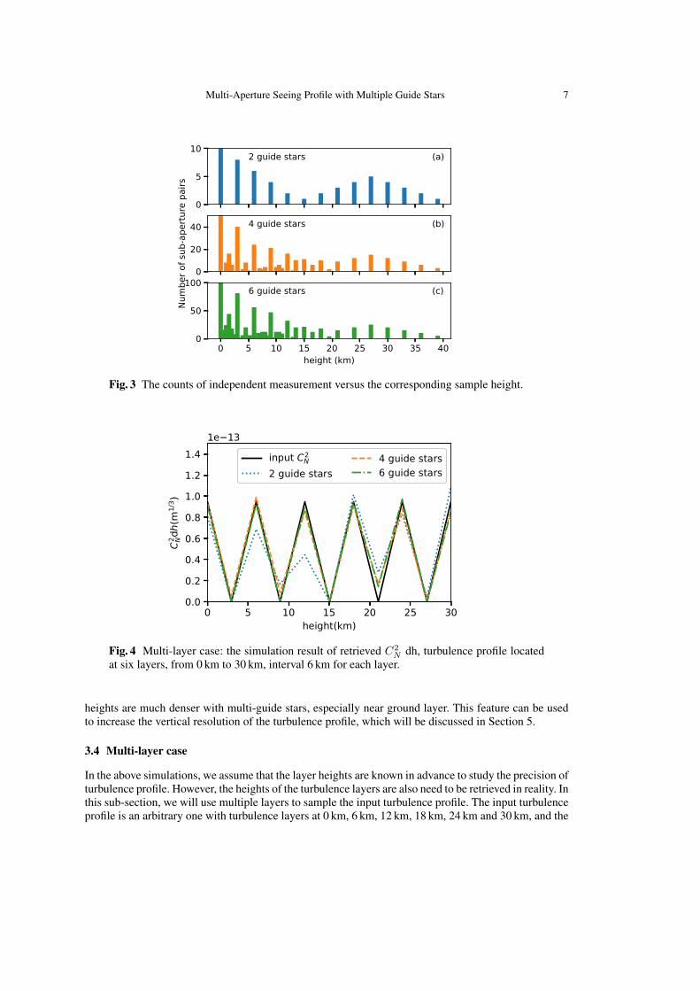
Multi-Aperture Seeing Profile with Multiple Guide Stars 7
0
5
10(a)2 guide stars
0
20
40
Numbe
r of s
ub-ape
rture pairs
(b)4 guide stars
0 5 10 15 20 25 30 35 40height (km)
0
50
100(c)6 guide stars
Fig. 3 The counts of independent measurement versus the corresponding sample height.
Fig. 4 Multi-layer case: the simulation result of retrieved C2
N dh, turbulence profile located
at six layers, from 0 km to 30 km, interval 6 km for each layer.
heights are much denser with multi-guide stars, especially near ground layer. This feature can be used
to increase the vertical resolution of the turbulence profile, which will be discussed in Section 5.
3.4 Multi-layer case
In the above simulations, we assume that the layer heights are known in advance to study the precision of
turbulence profile. However, the heights of the turbulence layers are also need to be retrieved in reality. In
this sub-section, we will use multiple layers to sample the input turbulence profile. The input turbulence
profile is an arbitrary one with turbulence layers at 0 km, 6 km, 12 km, 18 km, 24 km and 30 km, and the

8 F. Yang, G. Zhao & D. Q. Ren
1 3 542 10 12 141311
x
9876
y
Telescope 1 Telescope 2
w
Fig. 5 Similar as figure 1, but with smaller telescopes and bigger gap between the two tele-
scopes.
total r0 is 0.1 m. We use 11 layers located from 0 to 30 km with 3 km separation to sample the turbulence
profile. Namely, N = 11, and hn = n × 3 km in Equations 6 & 8. In the simulation, 4000 frames are
generated and used to retrieving the profile. In Figure 4, we plot the results. In the figure, black solid line
is the input C2
N , the blue dotted line,the orange dashed line, and the green dot-dashed line represents
the 2, 4 and 6 guide stars case, respectively. For the 2 guide stars case, we can see that layer at 12 km
can not be well measured. This is consistent with the results of Section 3.3 in which only one layer is
considered and the layer between 12 km and 18 km have large retrieving errors. We could also see that
the 4 guide stars and 6 guide stars case have similar performance and both provide precision turbulence
profile.
According to the atmospheric theories, there are high-altitude turbulence located at the tropopause
with altitude of about 9 - 18 km. However at these heights, the MASP instruments have large detection
errors if only two guide stars are used, since the sub-apertures corresponding heights are missing due
to the usage of two small telescopes. In this section, we found that if multiple guide stars are used, this
disadvantage of MASP will be overcome, and the turbulence layer at different heights can be measured
with high precision.
4 INCREASING THE SEPARATION OF THE TWO TELESCOPES OF MASP
In the original design of MASP with two guide stars, the separation between the two small telescopes
is restricted to be smaller than the diameter of the small telescope. Otherwise, turbulence layer around
certain height can not be detected. If multi-guide stars are used, fewer sub-apertures or lager separation
between telescopes is possible. In this section, we will test the turbulence profile retrieving process
using another configuration of the MASP with small telescopes and large separation , which is shown in
Figure 5. The size of each telescope is 320 mm, which is equal to 4w (4 sub-apertures are crossing the
aperture). The separation between the two telescopes is set to 480 mm (6w). The equivalent size of the
new configuration is still 1120 mm, same as the original one.
In Figure 6 the counts of independent measurement versus the corresponding sample height are plot-
ted, which is similar as Figure 3. In the new configuration, the maximum separation of sub-apertures
in single telescope is 3w, and the minimum separation of sub-apertures in different telescopes is 7w.
Therefore there is no sub-apertures pair with distance of 4w, 5w and 6w, and the corresponding tur-
bulence layers from 12 km to 18 km can not be measured (see panel (a) of Figure 6). While multiple
guide stars are used, the turbulence at 12 km, 15 km and 18 km can be measured using the combination
of (8w, 2∆α), (10w, 2∆α) and (12w, 2∆α), respectively. Thus we infer that the MASP with smaller
telescopes will have similar performance.
We repeat the numerical simulation in Section 3 to test the performance of the MASP with smaller
telescopes. In Figure 7, the results of one-layer case are plotted. From the Figure 7(a), we can see if
only 2 guide stars are used, r0 of the layers at about 15 km will have extreme large errors and can not be
measured. For the 4 guide stars and 6 guide stars case, the new configuration of MASP works well, and

Multi-Aperture Seeing Profile with Multiple Guide Stars 9
0
5
10(a)2 guide stars
0
20
40
Numbe
r of s
ub-ape
rture pairs
(b)4 guide stars
0 5 10 15 20 25 30 35 40height (km)
0
50
100(c)6 guide stars
Fig. 6 Similar as figure 3, while the guide star is two, the turbulence layers at 12 km to 18 km
can not be measured.
Fig. 7 Similar as figure 2, but when two guide stars are used, in some heights like 12 km, the
r0 can not be measured.
each layer can be retrieved with error < 7%. For both 4 stars case and 6 stars case, the standard error
curve also have a peak at about 15 km with value of 6.9% and 5.1%. Comparing with the results of the
standard MASP, which have maximum error of 5.5% and 3.2% for 4 and 6 guide stars, the precision of
new configuration are slightly lower but acceptable.
In Figure 8, we plot the simulation results that multiple turbulence layers are considered. The initial
setup is same as that in Section 3.4. 6 layers of input turbulence profile are considered in the simulation,
which are located from 0 km to 30 km, with separation of 6 km between two adjacent layers. For the
2 guide stars case (blue dotted line), turbulence layer at 12 km and 18 km can not be measured. The

10 F. Yang, G. Zhao & D. Q. Ren
Fig. 8 Similar as figure 4, while for 2 guide stars case, turbulence layer at 12 km and 18 km
can not be measured.
turbulence layer of these two layers are contributed to the lower layers, which leads to over estimated
of the strength of the lower layers. When we use 4 guide stars (orange dashed line), the C2
N can be well
retrieved. When 6 guide stars are used (green dot-dashed line), we will have a more accuracy result,
similar to the results of standard MASP.
In the new configuration of the MASP, two telescopes with diameter of 320 mm are used, and it have
similar performance wth the original design of MASP with 400 mm telescopes as well as a S-DIMM+
instrument on 1 m telescope with 14 apertures acrossing the diameter.
For a general case of MASP, we assume that the two telescopes have N apertures crossing their
diameters, and the separation of the two telescopes is equal to M times of the size of sub-aperture.
Using these assumptions, the distance between sub-apertures pairs in one telescope are from 1 to N −1,
while the distances between sub-aperture pairs at different telescopes are from M + 1 to 2N +M − 1.
If N − 1 ≥ (M +1)− 1 (namely M ≤ N − 1), the distances of sub-aperture pairs can be continuously
increased from 1 to M + N , and two guide stars are enough to sample the turbulence profile. In this
case two guide stars are used, the maximum equivalent diameter of the MASP is w(M + 2N) =(3N−1)w, which is about three times of the diameter of each telescope. If multiple guide stars are used,
we can have additional sampled heights using guide stars with larger angular separation. For example,
if the two guide stars have separations of 2∆α, additional sampled heights from w(M + 1)/(2∆α) to
w(2N+M+1)/(2∆α) can be used in the turbulence retrieving. These additional sampled heights would
cover the gap of sub-aperture distance, only if (2N +M − 1)/2 ≥ (M +1)− 1 and (M +1)/2− 1 ≤(N − 1). These two inequalities are equivalent to M ≤ 2N − 1, which means the maximum equivalent
diameter of the MASP with multiple guide stars is w(M + 2N) = (4N − 1)w, which is four times
of the diameter of the small telescope. Thus the equivalent diameter of the MASP will be increased by
(4N − 1− 3N + 1)/(3N + 1) ≈ 30%.
5 DISCUSSION
The vertical resolution of S-DIMM+ can be increased if multiple guide stars are used, which have been
well studied by the Wang et al. (2018). For the MASP, the vertical resolution can also be increased. In
Figure 3 and Figure 6, we can see that the heights grid are much denser if 4 or 6 guide stars are used. In
our pervious simulations of multi-layers cases, the height grid is a uniform one with vertical resolution
of 3 km, and vertical resolution could be increased if we use un-uniform sample grid. In Figure 9a,

Multi-Aperture Seeing Profile with Multiple Guide Stars 11
0 10 20 30 40height(km)
0
1
2
3
4
5
6
7
C2 Ndh(m
1/3 )
1e−13input C2
n
2 guide stars4 guide stars6 guide stars
0 10 20 30 40height(km)
0.0
0.5
1.0
1.5
2.0
2.5
3.0
3.5
4.0
vertica
l res
olution(km
)
2 guide stars4 guide stars
6 guide stars
Fig. 9 Increase the vertical resolution by using multiple guide stars. (a) the cumulated C2
Nd.husing different guide stars. (b) the vertical resolution at different height.
we plot the cumulated C2
Nd.h using different guide stars. The meaning of each curves is same as that
those of Figure 4 and 8 and the solid points indicate the height grid. It can be seen that with multiple
guide stars, the vertical resolution can be dramatically increased near ground. The vertical resolution at
different height are estimate in Figure 9b. If two guide stars are used, the vertical resolutions are 3 km
for all the layers. While multi-guide stars are used, the vertical resolution for the turbulence layer below
10 km is about 0.5 km - 1 km. If 6 guide stars are used, the vertical resolution can be as high as 0.2 km. In
the day-time, the cool nocturnal air warms up thus the turbulence near ground become stronger. Using
multiple guide stars, we can character the strong day-time ground turbulence layer better.
6 CONCLUION
Day-time turbulence profile is important for the design of both optics and control algorithm of solar
MCAO. Currently, S-DIMM+ is the most useful method to measure the day-time turbulence profile up
to 30 km. However, S-DIMM+ need to use a solar telescope with diameter of about 1 m, which limit the
usage of S-DIMM+ on site survey. The Multi-Aperture Seeing Profile (MASP) consists of two small
telescopes and is portable for site seeing test. Using the turbulence profile retrieving algorithm similar to
S-DIMM+, MASP can measure the turbulence profile up to 30 km. In the original design of MASP, only
two guide stars are used. In this paper, we aim to use multiple guide stars to improve the performance
of MASP.
We find that using multiple guide stars, the precession of turbulence profile by MASP can be in-
creased, especially for the turbulence layers at 12 - 18 km where the high altitude turbulence layer at the
tropopause are mainly located. Thus using multiple guide stars, MASP can provide better measurement
on the high-altitude turbulence.
A new configuration of MASP was introduced which is consisted of two 320 mm telescopes. If
multiple guide stars are used, it will have same equivalent diameter as the original design of MASP with
400 mm telescopes. This means using multiple guide stars, the equivalent diameter of MASP can be
increased up to 30%.
The vertical resolution of MASP is also studied. If multiple guide stars are used, the vertical reso-
lution near ground can be increased from 3 km to ∼ 0.5 km in our case of study. Thus the strong ground
turbulence at day-time can be better charactered.
12 F. Yang, G. Zhao & D. Q. Ren
Acknowledgements This work was supported by the NSFC (Grant Nos. 11873068, 11433007,
11661161011, 11673042), the Strategic Priority Research Program of the Chinese Academy of
Sciences (Grant No. XDA15010300), the International Partnership Program of Chinese Academy of
Sciences (Grant No.114A32KYSB20160018, 114A32KYSB20160057), the special funding for Young
Researcher of Nanjing Institute of Astronomical Optics & Technology and part of this work was carried
out at CSUN, with the support of NSF under grant AST-1607921.
References
Avila, R., Aviles, J. L., Wilson, R. W., et al. 2008, MNRAS, 387, 1511 2
Beckers, J. M. 1988, Very Large Telescopes and their Instrumentation, Vol. 2, 2, 693 1
Beckers, J. M. 2001, Experimental Astronomy, 12, 1 2
Butterley, T., Wilson, R. W., & Sarazin, M. 2006, MNRAS, 369, 835 2
Collados, M., Bettonvil, F., Cavaller, L., et al. 2010, Proc. SPIE, 7733, 77330H 2
Egner, S. E., & Masciadri, E. 2007, PASP, 119, 1441 2
Elmore, D. F., Rimmele, T., Casini, R., et al. 2014, Proc. SPIE, 9147, 914707 2
Johansson, E. M., & Gavel, D. T. 1994, Proc. SPIE, 2200, 372 5
Kellerer, A., Gorceix, N., Marino, J., Cao, W., & Goode, P. R. 2012, A&A, 542, A2 2
Kellerer, A. 2015, arXiv:1504.00320 4
Ren, D., Zhu, Y., Zhang, X., Dou, J., & Zhao, G. 2014, Appl. Opt., 53, 1683 1
Ren, D., Jolissaint, L., Zhang, X., et al. 2015, PASP, 127, 469 1
Ren, D., Zhao, G., Zhang, X., et al. 2015, PASP, 127, 870 2, 4, 5
Ren, D., & Zhao, G. 2016, PASP, 128, 105002 2, 5
Ren, D., Zhao, G., Wang, X., Christian Beck, Robert Broadfoot. 2018, Solar Physics, To be published.
2
Rimmele, T. R., Woeger, F., Marino, J., et al. 2010, Proc. SPIE, 7736, 773631 1
Rimmele, T. R., & Radick, R. R. 1998, Proc. SPIE, 3353, 72 1
Scharmer, G. B., & van Werkhoven, T. I. M. 2010, A&A, 513, A25 2, 3
Tokovinin, A., Le Louarn, M., & Sarazin, M. 2000, Journal of the Optical Society of America A, 17,
1819 1
Tokovinin, A., Kornilov, V., Shatsky, N., & Voziakova, O. 2003, MNRAS, 343, 891 2
Townson, M. J., Kellerer, A., Osborn, J., et al. 2014, Proc. SPIE, 9147, 91473E 2
Vernin, J., & Munoz-Tunon, C. 1994, A&A, 284, 311 2
Waldmann, T. A., Berkefeld, T., & von der Luhe, O. 2007, Optical Society of America, p. PMA3 2
Waldmann, T. A., Berkefeld, T., & von der Luhe, O., II 2008, Proc. SPIE, 7015, 70155O 2
Wang, Zh., Zhang, L., Kong, L., et al. 2018, MNRAS, 478, 2 2, 10
Wilson, R. W. 2002, MNRAS, 337, 103 2