Moody Oil What is Driving the Crude Oil Price?

Moody OilWhat is Driving the Crude Oil Price?

Abstract

The unparalleled surge of the crude oil price after 2003 has triggered a heatedscientific and public debate about its ultimate causes. Unexpected demand growthparticularly from emerging economies appears to be the most prominently sup-ported reason among academics. We study the price dynamics after 2003 in theglobal crude oil market using a structural VAR model. We account for structuralbreaks and approximate market expectations using a time series for media senti-ment in order to contribute to the existing literature. We find that forward-lookingdemand activities rather than demand arising from real economic activity haveplayed an important role for the run-up in the price of crude oil after 2003. We ad-ditionally find that emerging economies have not majorly contributed to the pricesurge.

JEL classification: Q43; Q41; C32; D8; E3

Keywords: Oil Price; Spot Market; Futures Market; Fundamentals; Speculation; Financialization

1 Introduction

The increase in the price of crude oil in the first decade of the new millennium has caused

an extended debate about its reason. Three explanations are usually outlined in this

context: First, it is claimed that the rising price reveals the finiteness of crude oil and the

inability to further extent production capacities (supply-driven price increase). Second,

it is hypothesized that the unexpectedly strong growth of emerging countries such as

China and India has resulted in an unexpected increase of crude oil demand, leading to

squeezes in the spot delivery of crude oil and a rising price (demand-driven price increase).

Third, it is stated that the increasing number of speculators in the market of crude oil

has considerably enforced the role of forward-looking demand activities and therewith

altered the price dynamics (expectation-driven price increase).

Amongst the three explanations, the demand hypothesis has been averted most (Kil-

ian (2009), Kilian and Murphy (2010), Kilian and Hicks (2012), Krugman (2008) and

Hamilton (2008, 2009)). The supply hypothesis, as well as the expectation hypothesis

have seen a less pronounced echo in the literature (see e.g. Kaufmann, 2011 for arguments

in favor of the supply hypothesis and Singleton, 2011, and Hamilton and Wu, 2011, find

speculation as a main driver of the price increase).

The major challenge in empirically assessing which of the three hypotheses provides

a better explanation for the dynamics in the crude oil market after 2003 consists in

isolating the different forces in its effect on the price. While price effects arising from

supply are identifiable due to the ability of observing extracted quantities of crude oil, a

differentiation between the remaining two potential causes of the price increase requires a

careful decomposition of observed total crude oil demand into two ”un-observable” parts:

fundamental crude oil demand, i.e. demand for crude oil today that arises as a result

of today’s real economic needs for the commodity, and forward-looking demand which

is triggered by the expectation of changes in the market of crude oil taking place in the

future.1 Both types of demand need to be approximated by suitable data. As changes

1As crude oil is storable, it is possible to buy or sell units of crude oil in the future or spot market in

1

in the fundamental demand for crude oil mainly arise due to up- and downturns of the

business cycle, it can be represented by appropriate business cycle indicators. However,

an approximation of forward-looking demand is far less straightforward: such activities

are driven by expectations and thus not directly observable. Inventories as an outcome of

expectation-driven demand, in contrast, is observable but data are generally considered

not reliable. Thus, approximating forward-looking demand in empirical models on the

oil market is still an open issue.

Several approaches have been taken in the literature to proxy for forward-looking

demand. While Kilian (2009) relegated all expectation-driven demand activities into

the residuum, subsequent papers in this strand of literature have tried to find explicit

proxies for this variable. Kilian and Murphy (2011) consider shocks to OECD crude

oil inventories as a mean of capturing changes in market expectations.2 This approach,

however, requires that OECD inventories data are correct, provided in a timely fashion

and that they resemble activities of all market participants, including investment banks

and growing economies such as China and India (see e.g. Singleton, 2011 on the limits

of inventory data).

In this paper, we contribute to the question of what has driven the price of crude oil

after 2003 by considering a new means of representing forward-looking demand. In order

to proxy for forward-looking crude oil demand, we use a time series of all news items with

reference to the crude oil market that have appeared on news tickers of one of the world’s

largest news suppliers. The qualification of such a time series to be used as a proxy for

forward-looking demand is rooted in the principles of economic theory according to which

information serves as foundation for expectation formation (see e.g. Muth, 1961). As this

time series reconstructs the continuous flow of information to the crude oil market, it is

indicative of market expectations and consequently of forward-looking demand activities.

With this new proxy for forward-looking demand for crude oil at hand, we undertake

a structural decomposition of the crude oil price in a VAR model. The methodology

expectation of future market conditions. Thus, the price reflects current conditions as well as expectationsof future market conditions. Note that such forward-looking demand activities incorporate anticipativedemand activities related to future real economic needs as well as demand activities anticipating futureprice movements but unconnected to real needs.

2The rational is that ”any expectation of a shortfall of future oil supply relative to future oil demandnot already captured by flow demand and flow supply shocks necessarily causes an increase in the demandfor above-ground oil inventories and hence the price of crude oil” (pg. 2).

2

follows Kilian (2009).

Results of the structural VAR model show that the price development is mainly de-

scribed by shocks from news sentiment, indicating that forward-looking demand activities

have played a crucial role. As these results stand in contrast to previous contributions on

this topic, we provide an extended sensitivity analysis in which we discuss possible trig-

gers of our results, such as structural breaks in the time series, variations in the proxy for

fundamental demand and the role of emerging economies for the global crude oil demand.

In particular, we find evidence that structural breaks have occurred in the global crude

oil market in 2003 which is crucial for the estimation results. Furthermore, we find no

empirical support that current real economic activity in major emerging economies has

driven the price surge after 2003. Thus, we conclude that the crude oil price development

reflects the anticipation of future market fundamentals. In other words, it has been the

expectation of future market conditions rather than unexpected shocks to current market

conditions that explain the price movements.

2 The Empirical Model

In the following section, we propose a four-dimensional structural VAR (SVAR) model for

the time period of 2003-2010. The model incorporates an explicit differentiation between

fundamental and forward-looking demand.

2.1 Model Description and Identification

The price of crude oil is set in the global market and is therefore simultaneously deter-

mined with other macroeconomic aggregates which complicates the identification process

of the model’s parameters. SVAR models provide a suitable approach in this context as

they consist of endogenous variables only and, thus, do not require exogenous variables for

identification. In return, the identifying strategy relies on restrictions imposed on the in-

terplay of the variables under consideration. These restrictions typically cannot be tested

and should therefore rely on a sound theoretical fundament. The empirical results are

derived by modeling and analyzing unobserved structural shocks using impulse-response

functions and cumulative effects of these shocks on the variables of interest.

Starting point for the estimation of an SVAR model is the estimation of its reduced

3

form, i.e. a conventional VAR model, using OLS estimation methodology. The VAR

model is based on monthly data for

yt = (prodt, econactt, sentimentt, pricet)′

where prodt is the percentage change in global crude oil production, econactt refers to the

economic activity index, sentimentt denotes the time series of news sentiment reflecting

expectation based market activities and pricet is the real price of crude oil. The number

of lags, p, is chosen to be nine.3 The VAR representation is

yt =9∑

i=1

Aiyt−i + et. (1)

The underlying SVAR models the contemporaneous effects between the variables yt

A0yt =9∑

i=1

A∗i yt−i + εt (2)

with Ai = A−10 A∗i and et = A−10 εt.

The structural parameters cannot be identified without imposing restrictions on the

model. While there are in general several techniques of how to impose such restrictions,

we apply a parametric approach which is based on a recursive system.4 We reduce the

number of free parameters by imposing a triangular structure on the matrix A0. We

impose the following restrictions:5

et =

eprodt

eeconactt

esentimentt

epricet

=

a11 0 0 0a21 a22 0 0a31 a32 a33 0a41 a42 a43 a44

εflow supply shockt

εflow demand shockt

εnews shockt

εresidual shockt

. (3)

In contrast to the reduced form disturbances et from the VAR model which are only

linear combinations of the unidentified structural innovations εt, residual shocks from the

structural model can now be interpreted in a meaningful economic way. Flow demand and

3See Section 2.6 for a justification of the choice of the number of lags.4Recursivity typically requires two types of assumptions: First, the structural shocks are assumed

to be uncorrelated, i.e. the variance-covariance matrix Σε is diagonal. The underlying economic in-terpretation is that the structural shocks do not have a common cause. Second, restrictions on thecontemporaneous relationships of variables are imposed. Further methods for recovering structural pa-rameters are long-run restrictions or sign restrictions. For more details on identifying restrictions see Fryand Pagan (2009).

5With the model being four-dimensional (K = 4), we set K(K−1)2 = 6 elements of matrix A0 equal

to zero. The restrictions described in Equation (3) follow the justifications given in Kilian (2009).

4

flow supply shocks represent unexpected changes in fundamental market forces whereas

the news shock depicts changes in the forward-looking demand-component. The SVAR-

parameters are determined using Maximum-Likelihood methodology. All estimations are

conducted in R, version 2.12.2 (R Development Core Team, 2011).

2.2 News Sentiment as Estimate for Forward-Looking Demand

While current needs of crude oil contribute to total crude oil demand and thus to the

price formation, the ability to store crude oil allows agents to act today to tomorrow’s

expected changes in the market of crude oil.6 Thus, the spot price of crude oil contains

views held in the market place regarding the future conditions of supply and demand

in addition to current supply and demand conditions. Such expectation-based demand

activities need to be explicitly modeled to correctly represent the relative contribution of

each force to the price development.

A direct way of capturing expectations held in the market place consists of going to the

roots of the expectation formation process. What affects the formation of expectations

in the market? According to economic theory, the process is based on information that

market participants receive over the course of time (Muth, 1961). Thus, a time series

that captures in a continuous way all pieces of information that are relevant for the crude

oil market is indicative for the expectations of market participants regarding the future

development of supply and demand.7

The Thomson Reuters News Analytics Database allows a re-construction of the con-

tinuous flow of information to the market. It contains all news items that have run over

tickers in trading rooms. Time stamps characterizing the exact time of appearance of the

news item as well as topic codes describing topics mentioned in the text allow for a selec-

6Expectations regarding the future development of supply and demand impact the price of crude oilthrough two channels: On the one hand, the price for a future delivery of crude oil can be agreed upontoday on futures markets. On the other hand, crude oil is storable so that market participants can buyunits today in anticipation of future market conditions. Thus, if an individual, for example, holds theexpectation of a rising crude oil demand in the nearer future, she may take precautionary steps to avoidhaving to pay a high price in the future. She can either decide to buy a futures contract today (if thecurrent futures price is still less than what she expects the spot price to be in the future) or buy crudeoil today and store it. In both cases, her expectation of the future conditions of demand and supply willhave an impact on the price of crude oil today, either via the futures market (and consequently, via theno-arbitrage condition also on the spot price) or via the spot market, directly.

7News have been used to model the formation of expectations in other contexts as well, see e.g. Lamlaand Sarferaz (2012).

5

tion of relevant news articles for the crude oil market and a construction of a continuous

time series of news items. Due to the broad coverage the database is representative of the

timely, public information available at least to professional investors, i.e. public news.

The language used to describe the content, i.e. news sentiment, helps in quantifying the

otherwise not quantifiable information of the news article.

Quantifying the content of a news article based on its language is a relatively new

approach and has become possible through the advent of automated linguistic programs.

The idea behind the program is that the overall tone of the language provides an indication

of the expected movement of the underlying economic variable. For example, news articles

reporting about an increase (decrease) of the economic variable referred to in the text

naturally use more positive (negative) words. Thus, an article reporting about an increase

(decrease) in supply or demand of crude oil can be expected to have been ascribed a

positive (negative) sentiment. Articles reporting about an increase in supply or demand

include news about an increase in OPEC supply, the finding of additional oil fields or an

increase in world economic growth. In contrast, news articles reporting about a reduction

in supply or a decrease in demand include articles on a war in resource rich countries, a

reduction in the supply from OPEC countries, riots or strikes on oil platforms or upcoming

economic recessions.

The sentiment attached to each news item is based on the tone of the language in

each individual news article: On the basis of large dictionaries, the program counts the

number of positive, negative and neutral words in each article and attaches a ”1” (”-

1”; ”0”) if the number of positive (negative/neutral) words outweighs the negative or

neutral ones. Additional information on the likelihood of whether the sentiment variable

correctly represents the tonus in the news article is given in form of probabilities (probpos

and probneg). The time series of daily sentiment is computed in the first step as

sents =∑

(1) × probpos +∑

(−1) × probneg. (4)

A time series of monthly sentiment is given as the sum of daily news sentiments.

Figure 1 shows the development of the crude oil price and the sentiment over time.

Since 2003 the price of crude oil and the news sentiment have shown a high degree of

co-movement: both, the time series of sentiment and the time series of the crude oil price,

6

are increasing until the outbreak of the financial crisis and abruptly decreasing at the

beginning of 2009. The years afterwards are characterized by a raising sentiment and

price. The synchronous development of the two time series manifests itself in a high,

positive correlation (0.815).

−0.0

10.

010.

02

Ser

ies

1−3

000

−100

010

00

Ser

ies

2−2

000

2000

6000

Ser

ies

350

100

150

200

250

2003 2004 2005 2006 2007 2008 2009 2010

Ser

ies

4

Time

data.ts

Figure 1: Development of crude oil price in comparison to news sentiment

There are several obstacles associated with using this time series as a proxy for market

expectations.

First, while the tone contains a signal regarding the expected change in supply or de-

mand of crude oil, news items lack a reference to which economic variable they correspond

to in particular. That is, we cannot observe a time series of news sentiment for supply

and demand, separately. Still, we can derive some conclusions regarding the relative im-

portance of supply- and demand-related news from descriptive statistics.8 First, as we

can observe whether news within a certain time period has been overly positive, negative

or neutral and as we can observe the direction of the price, it is possible to ex-post infer

the dominating type of news. As the correlation between the price of crude oil and news

sentiment has been positive, it is clear that the time series cannot consist of a dominating

number of references to supply. Furthermore, the news sentiment time series is highly

correlated with the level of OECD production as measured by the index of industrial

production provided by the OECD (0.765). Last, the application of a refined linguistic

8Note that estimated coefficients therefore will only reveal the average marginal effect of supply anddemand-related expectations on the price of crude oil.

7

selection method further clarifies the importance of demand and supply related news. In

order to approximate supply-related news sentiment (supsent) we filter news item based

on the word OPEC representing exogenous changes in production which did not respond

to current economic activity.9 Demand-related news sentiment (demsent) is identified

by selecting news items related to economic indicators. The correlation as well as the

multiple regression in Table 1 reveal that the supply-related news sentiment is not signifi-

cantly linked to the general crude oil market news sentiment (sent). The demand related

news sentiment, however, is significantly and positively linked to the crude oil sentiment

which indicates that its content is governed by demand-related information. Based on

the development of the sentiment and price time series, the question remains whether

these news articles rather describe current conditions of the market or whether the news

have resulted in the formation of certain expectations that were not accompanied by a

corresponding shift in flow demand or flow supply. The structural VAR decomposition

where we account for fundamental supply and demand will allow for such a separation of

effects.

The second issue regarding the use of news sentiment as proxy for market expectations

relates to the question how many news items simply contain reports of the current de-

velopment of the crude oil price, without further information on demand or supply. One

could claim that the strong co-movement of the two time series and their high correlation

is indicative of this hypothesis. The problem at the heart of this issue is the one of cause

and effect between news sentiment and the price of crude oil. We shed some light on this

causality by applying a bivariate Granger-Causality-Test. We find that, on a monthly

basis, changes in news sentiment precede corresponding crude oil price dynamics.10

2.3 Motivation & Implications of Restrictions

The restrictions imposed on the contemporaneous relationships of the four variables in

Section 2.1 are explained in the following section.

Restrictions on Crude Oil Production

9Note that this is just one type of supply related news. A further refinement is work in progress.10Note that this is work in progress for a separate paper. Preliminary results can be obtained from

the authors upon request.

8

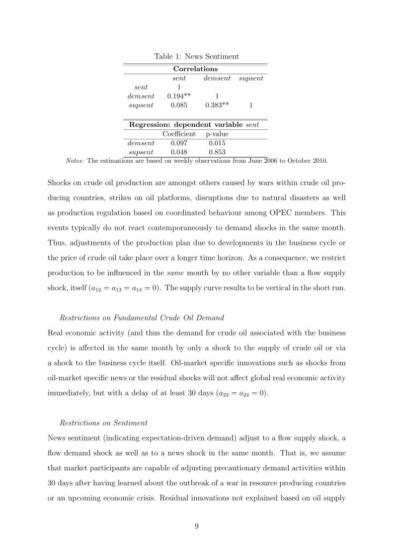
Table 1: News Sentiment

Correlations

sent demsent supsentsent 1

demsent 0.194** 1supsent 0.085 0.383** 1

Regression: dependent variable sent

Coefficient p-value

demsent 0.097 0.015supsent 0.048 0.853

Notes: The estimations are based on weekly observations from June 2006 to October 2010.

Shocks on crude oil production are amongst others caused by wars within crude oil pro-

ducing countries, strikes on oil platforms, disruptions due to natural disasters as well

as production regulation based on coordinated behaviour among OPEC members. This

events typically do not react contemporaneously to demand shocks in the same month.

Thus, adjustments of the production plan due to developments in the business cycle or

the price of crude oil take place over a longer time horizon. As a consequence, we restrict

production to be influenced in the same month by no other variable than a flow supply

shock, itself (a12 = a13 = a14 = 0). The supply curve results to be vertical in the short run.

Restrictions on Fundamental Crude Oil Demand

Real economic activity (and thus the demand for crude oil associated with the business

cycle) is affected in the same month by only a shock to the supply of crude oil or via

a shock to the business cycle itself. Oil-market specific innovations such as shocks from

oil-market specific news or the residual shocks will not affect global real economic activity

immediately, but with a delay of at least 30 days (a23 = a24 = 0).

Restrictions on Sentiment

News sentiment (indicating expectation-driven demand) adjust to a flow supply shock, a

flow demand shock as well as to a news shock in the same month. That is, we assume

that market participants are capable of adjusting precautionary demand activities within

30 days after having learned about the outbreak of a war in resource producing countries

or an upcoming economic crisis. Residual innovations not explained based on oil supply

9

shocks, aggregate demand shocks or news shocks are excluded from affecting news senti-

ment within the same month (a34 = 0).11

The Price of Crude Oil

Last, the price of crude oil is the most reactive variable within the system as it responds

instantaneously (i.e. within the same month) to flow supply, flow demand, news shocks

and shocks that are not captured by any of the other three types of shocks (residual

shocks).

2.4 Data

We use monthly global crude oil production taken from the Energy Information Admin-

istration (EIA) as measure of crude oil supply. The refiner acquisition cost of imported

crude oil, deflated by the US CPI and expressed in logs, is taken as proxy for the real price

of oil. We employ the index of industrial production as provided in the MEI database of

the OECD as measure of business-cycle related crude oil demand. Last, we use the sen-

timent time series for the crude oil market as obtained from the Thomson Reuters News

Analytics database, expressed in logs, as explicit measure for precautionary demand ac-

tivities. The data run from February 2003 until February 2010. As the time series of the

OECD production indicator as well as the one for crude oil production contain a unit

root (see Table 3 in the Appendix), we transform the time series from levels into growth

rates in order to achieve stationarity. While the crude oil price also exhibits a unit root,

we restrain from any further transformation to preserve the information contained in the

levels of the time series.

2.5 Results

Figure 2 represents the responses of the price to a unit shock from each of the four

variables.12 They allow four conclusions.

11Note that the bivariate Granger-causality test provides support for this restriction: changes in newssentiment precede corresponding crude oil price dynamics on a monthly basis.

12The impulse response functions for the response variables supply, demand and news are shown inthe Appendix (Figure 11 to 13).

10

First, the responses of the crude oil price to a shock from flow supply and flow de-

mand exhibit economically plausible patterns: A flow supply shock has a negative (not

significant) impact on the price of crude oil after around nine months. A flow demand

shock leads to a positive and significant increase in the price of crude oil, peaking after

about eight months.

Second, a news shock has a highly significant and positive impact on the price of crude

oil. The effect is significant from the impact period onwards and lasts for the following

five months. A positive shock from news accordingly represents the expectation of higher

demand in the future. This indicates that forward-looking demand activities have taken

place, resulting in an increase in the price of crude oil. Note that a news shock does not

have a reverting behavior of the price of crude oil. It remains positive over the course of

the following 18 months.

Third, the results also indicate a reasonable difference in speed in the adjustment

of the price of crude oil to flow demand and news shocks: while flow demand shocks

arising from the business cycle need more than half a year to fully unfold their impact,

news shocks have a rather short term impact on the price of crude oil with no significant

influence after half a year.13

Last, residual shocks do also impact the price of crude oil significantly but show

signs of self-reverting behavior. While a residual shock increases the price of crude oil

significantly during the first two to three months, the shock turns negative over the

following months.

In accordance with the results from the impulse response functions, the historical

decomposition of the price of crude oil in Figure 3 attributes most of the price development

to news shocks. Especially around the year 2008, expectation-driven demand activities

have influenced the price of crude oil in a notable way. While shocks from flow demand

can explain some swings in the price of crude oil, they did not contribute in a systematic

way. Flow supply shocks did not help to explain the price development, at all.

Last, cumulative effects from residual shocks are rather volatile but do not show a

systematic pattern. This is in line with the overshooting pattern found in the impulse

13Adjustments to shocks from fundamental demand are clearly more sticky than adjustments to ex-pectation shocks. While the latter does include costs from adjusting positions in the futures markets oradjusting inventories, the first incurs other costs, such as capacity adjustments.

11

Pri

ce

SVAR Impulse Response from Supply

90 % Bootstrap CI, 2000 runs

0 2 4 6 8 10 13 16

−2

.0−

1.0

0.0

1.0

Pri

ce

SVAR Impulse Response from Demand


0 2 4 6 8 10 13 16

−1

01

2

Pri

ce

SVAR Impulse Response from News


0 2 4 6 8 10 13 16

−0

.15

−0

.05

0.0

50

.15

Pri

ce

SVAR Impulse Response from Price


0 2 4 6 8 10 13 16

−0

.10

0.0

00

.10

Impulse Response Functions

Figure 2: Impulse response function for the Crude Oil Price

Cumulative effect of flow supply shock on crude oil price

2005 2006 2007 2008 2009 2010

−0.

40.

2

Cumulative effect of flow demand shock on crude oil price

2005 2006 2007 2008 2009 2010

−0.

40.

2

Cumulative effect of news shock on crude oil price

2005 2006 2007 2008 2009 2010

−0.

40.

2

Cumulative effect of residual shock on crude oil price

2005 2006 2007 2008 2009 2010

−0.

40.

2

Figure 3: Historical decomposition of crude oil price in four variables model

12

response function according to which the shocks did not have a persistent effect on the

price of crude oil.

All in all, the results from the SVAR model do not support the hypothesis that

unexpected shocks from real economic activity have caused the increase in the price of

crude oil after 2003. Rather, they suggest that the price surge was mainly driven by news

shocks, i.e. shocks to expectations regarding future market conditions.

2.6 Diagnostic testing

The results of an SVAR model do not only depend on the choice of the identifying

assumptions but also on the specification of the underlying reduced-form model. Whereas

the assumptions are imposed on the model on a priori grounds and cannot be tested

directly, there are various statistical procedures for examining whether the reduced-form

specification adequately represents the data generating process (DGP). In this section,

following Breitung, Bruggemann, and Lutkepohl (2004) or Pfaff (2008), we apply some

well established diagnostic procedures.

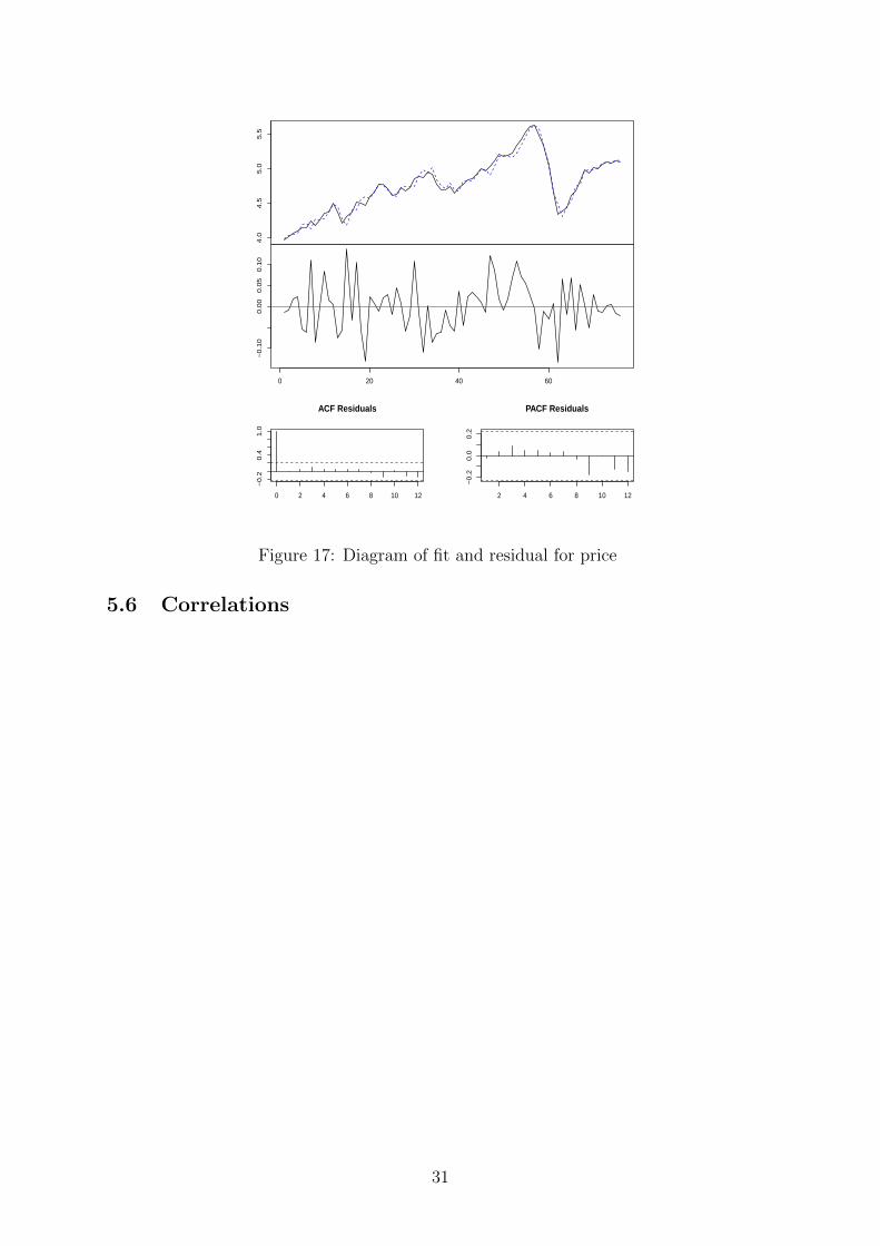
Figure 14 to 16 in the Appendix display the diagram of fit and the residual for every

variable in the VAR model - flow supply, flow demand, news and crude oil price. Based on

visual assessments, the plots of the residuals do not indicate any noticeable specification

problems. In addition, the estimated autocorrelation function (ACF) as well as the partial

autocorrelation function (PACF) for each single residual does not exhibit any significant

deviation from zero at any lag.

In the following we apply multivariate tests to the model residuals. In a first step

we test for the absence of autocorrelation. Two different procedures are considered: we

perform a test based on an adjusted portmanteau statistic Qh in order to check the null

hypothesis of no autocorrelation against the alternative that at least one autocovariance

is nonzero.14 Secondly, as described in Godfrey (1978), we apply the Breusch-Godfrey

LM (BP) statistic in order to test for hth order autocorrelation. As we can see from

Table 2 both tests reject the null hypothesis of no autocorrelation in the model residuals.

While a higher number of lags may reduce autocorrelation, the number of observations in

our dataset imposes a severe trade-off in terms of asymptotic properties of the estimated

14For a more detailed description of the following test statistics see Lutkepohl (2004).

13

parameters. Tests on optimal lag length (i.e. the Akaike information criterion (AIC),

the Hannan-Quinn criterion (HQ) and the Schwarz criterion (SC)) indicate only little

informational gain for lag three and beyond (see Table 2). In order to find a compro-

mise between the optimal lag length, the autocorrelation patterns and the suggestion

in previous papers of including long lag orders (e.g. Hamilton and Herrera (2004) and

Kilian (2009)), we increase the corresponding number up to nine in order to adequately

represent the dynamics of the global crude oil market.

In a further step, we test for conditional heteroskedasticity in the error term by

applying a multivariate extension of the univariate ARCH-LM test as described in Engle

(1982). The corresponding p-value from Table 2 indicates that no ARCH effects are

present.

Finally, we test for nonnormality in the error term. The test is based on the skewness

and kurtosis properties and is constructed by generalizing the Lomnicki-Jarque-Bera (JB)

test (Jarque, Bera; 1987). As we can see from Table 2 the null hypothesis of the residuals

being normally distributed cannot be rejected. Based on the test results we conclude

that the reduced-form model performs in a satisfactory manner, providing an adequate

basis for the structural identification.

Table 2: Model Checking: the VAR Specification

Diagnostic Tests

Qh p-value BG p-value ARCH p-value JB p-value

164.029 0.001 147.866 ≤ 2.2e-03 512.845 0.336 2.250 0.972

Lag Length Selection

AIC lag length HQ lag length SC lag length

-28.416 2 -28.002 1 -27.634 1

3 Discussion

What has caused our results to differ so dramatically from those obtained in the reference

literature? In the following section, we provide a discussion about possible factors causing

the difference, e.g. the time period of estimation and the choice of the fundamental

demand indicator. Last, we examine whether we can find empirical support for the

hypothesis of demand from emerging economies triggering the price increase as it provides

14

the backbone of the demand growth hypothesis.

3.1 Fundamental Changes and Structural Breaks

The first difference of our model in comparison to the estimations in the reference litera-

ture arises from the estimation horizon. We use data starting in 2003 due to the limited

availability of the Thomson Reuters News Sentiment time series while many empirical as-

sessments of the crude oil market use data over several decades. While longer time series

are usually preferred as asymptotic properties of estimators increase with the number of

observations, the likelihood of encountering structural breaks in the time series rises with

the number of observations, as well. Ignoring the presence of such discontinuities when

estimating a structural VAR model renders wrong parameter estimates and thus results.

The finding of structural breaks occurring around 2003 would justify the concentration

of our estimations on the shorter time horizon.

Various contributions have documented an altered functioning of the market for crude

oil after 2003, indicating the likelihood of altered properties of the underlying time series

(see e.g. Tang and Xiong (2011), Hamilton and Wu (2011)).

In order to find out whether central variables related to the market for crude oil have

indeed experienced structural breaks within recent decades, we have applied a three-step

test procedure to data most often used in the reference literature on oil price decomposi-

tions, i.e. Drewry’s shipping index as proxy for business-cycle related demand, crude oil

supply and the spot price of crude oil.

In the first step, we investigate for the three time series whether the mean differs

significantly for sub-periods of the sample.15 We compute an F-statistic in order to

compare the unsegmented model against a possible break for each point in time. Following

Andrews and Ploberger (1994), we reject the null hypothesis of structural stability if the

supremum of these statistics is too large. We reject the null hypothesis of no structural

change for the mean of shipping and the mean of the price at the 5% level. In order

to see at which points in time the null hypothesis is rejected, we draw the process of

the F-statistics for shipping and pricing (Figure 4), where the peaks roughly indicate the

15The data start in January 1973 and end in November 2007. For a detailed description of the datasee Kilian (2009).

15

timing of possible structural shifts. The straight line illustrates the threshold for rejecting

the null hypothesis. The process for shipping has three peaks: at the beginning in 1973,

around 1982, and around 2004. The F-statistics for the price variable exhibit one peak

around 1985 and one around 2003.

Shipping

Time

F st

atis

tics

1980 1985 1990 1995 2000 2005

040

80

Price

Time

F st

atis

tics

1980 1985 1990 1995 2000 2005

010

025

0

F statistics

Figure 4: The process of the F-statistic

Given the evidence for structural instability for two time series, we assess the timing

of the structural break following the procedure described in Bai and Perron (2003) in the

next step. We assume a three-segment partition with two breaking points for both means

based on the behavior of the F-statistics described above. The mean of the shipping

variable contains breaking points in November 1981 and February 2003. The mean of the

price variable occurs several months later, i.e. December 1982 and May 2003. Figure 5

illustrates the timing of the structural breaks and the mean for each sub-period for the

time series of economic activity (”shipping”) and the real price of oil.

In a last step we find that the null hypothesis of no structural break in May 2003

is clearly rejected (test-value=932.910, p-value ≤ 2.2e-03) by applying a Chow test for

structural breaks to the VAR model including the three variables under examination.16

16For a detailed description see Lutkepohl (2004).

16

In summary, we find that the single time series of the spot crude oil price and of the

economic activity indicator, as well as the structural VAR model representing the global

crude oil market, exhibit a structural break in 2003.

This finding implies the need to focus on sub-periods for estimations that coincide

with our chosen estimation period.17

The importance of acknowledging the presence of structural breaks in the estimations

can be highlighted when re-estimating Kilian (2009) for the estimation period of 2003-

2010. Focussing on this sub-period, results change dramatically: Not business-cycle

related demand as in Kilian (2009), but forward-looking demand activities seem to have

been the main driver of the price development of crude oil after 2003 (see Section 5.1 of

the Appendix). Thus, the consideration of structural instability seem important in an

empirical assessment of the crude oil market.

Shipping

Time

1975 1980 1985 1990 1995 2000 2005

−40

040

80

Price

Time

1975 1980 1985 1990 1995 2000 2005

−10

00

50

Visualization Breakingpoints

Figure 5: Breakingpoints and mean of sub-seriods

17Similar conclusions with respect to the occurrence of structural breaks are drawn in a variety of othercontributions. Fan and Xu (2011) find three structural breaks which have occurred since the start of thenew millennium: a ”relatively calm market” period (January 07, 2000, to March 12, 2004); the ”bubbleaccumulation” period (March 19, 2004, to June 06, 2008,); and the ”global economic crisis” period (June13, 2008, to September 11, 2009). Further evidence of a change in the dynamics of the crude oil marketis provided by Kaufmann (2011) who documents a structural break in the series on U.S. private crudeoil inventories.

17

3.2 The Indicator for Business-Cycle Related Crude Oil De-mand

A second source of variation of our model in contrast to the reference literature consists

in the choice of the proxy for business-cycle related crude oil demand.18 The reference

literature has mainly used fundamental demand proxies based on shipping activities, i.e.

the Baltic Dry Exchange Index or Drewry’s shipping index, in order to infer crude oil

demand associated with real economic activity. However, while one would expect an

estimate of business-cycle related crude oil demand to be correlated with either total

crude oil demand or other indicators of the business cycle, we do not find a significant

correlation with the commonly used estimators for the time period of 2003-2010: The

correlation between the Baltic Dry Exchange and two alternative business cycle indica-

tors, the index of industrial production (IIP) provided in the MEI database of the OECD

and the Composite Leading Indicator (CLI) provided by the OECD, is -0.028 and 0.21,

respectively, and not significant. In addition, the shipping indicator does not show any

relation to figures on total crude oil demand, either (0.045, not significant).19 Due to

these obvious shortcomings, we have used the index of industrial production which is

positively and significantly correlated with total crude oil demand (0.381).

The reference literature has refrained from using indices based on industrial produc-

tion to proxy for crude oil demand associated with real economic activity due to several,

presumed shortcomings (see Kilian, 2009). We argue, however, that they are not severe

in the context of our estimations: First, the link between fundamental crude oil demand

and industrial production figures has been argued to be influenced by structural changes

of economies and the development of new technologies. While this argument applies

in particular to estimations conducted over several decades, it may be less problematic

when investigating only a period of several years. Second, it has been argued that data

on industrial production are only available for a fraction of countries in the world. For

example, industrial production of major emerging economies are not yet contained in

18It has become common practice to identify fundamental crude oil demand with the help of businesscycle indicators. Such indicators are capable of indicating changes in the demand for crude oil that arepurely based on an expansion or contraction of current world economic activity and thus demand forcrude oil for today’s use. Note that there are some crude-oil intensive activities that are not closelyrelated to industrial production, e.g private traveling. However, such activities can be assumed to behighly correlated with the overall business cycle.

19The correlation-coefficients for all relevant variables are listed in Table 4 in the Appendix.

18

standardly available indices. Still, we find that countries for which data on industrial

production is provided contribute on average by 77% to total world GDP between 2003

and 2010. China and India only contribute by 8% to world GDP.20

Replacing the shipping index in the estimations of Kilian (2009) by the index of

industrial production as provided by the OECD for the time period of 2003-2010, we

find that the latter provides a better explanatory power for the price than the shipping

indicator.21 The results of the estimation are shown in Figure 9 and Figure 10 in Appendix

5.2.

The overall conclusion from the structural decomposition using the alternative proxy

for fundamental demand remains the same: forward-looking demand shocks have mainly

contributed to the price increase after 2003 (Figure 10). Thus the results obtained in

Section 3.1 are robust to the choice of the demand indicator.

3.3 The ”China-Effect” - The Role of Emerging Economies forthe Development of the Crude Oil Price

As a last sensitivity analysis, we investigate the demand growth hypothesis in greater

detail, i.e. the claim that demand from emerging economies such as China and India has

driven the price increase in 2003.

We re-run the model in Section 2 but replace the industrial production indicator for

OECD countries by two sorts of leading indicators: the first composes of only OECD

countries, the second additionally includes major non-member economies (MNEs), in-

cluding China, India, Russia, South Africa and Indonesia.

Note that due to the characteristics of a leading indicator these results will be only

informative with respect to a comparison of cumulative effects of flow demand shocks.

The results cannot be used as a comparison of the role of fundamental versus forward-

looking demand for the price development as the leading indicator contains expectations

regarding the development of the business cycle. The leading indicators therefore capture

part of the information contained in the news sentiment time series.

20However, looking at GDP increases only, emerging countries play a more prominent role: between2003 and 2010 China and India contribute to global increase in GDP by an average of 30%, whereas thecontribution from the OECD is 42%.

21The shocks from the industrial production indicator on the price appear to be partly significant incontrast to shocks from the shipping indicator. As in Section 3.1, the industrial production indicator isconsidered in growth rates rather than levels.

19

Cumulative effect of oil supply shock on real price of crude oil

Time

2005 2006 2007 2008 2009 2010

−1.0

0.0

1.0

Cumulative effect of aggregate demand shock on real price of crude oil

Time

2005 2006 2007 2008 2009 2010

−1.0

0.0

1.0

Cumulative effect of speculative demand shock on real price of crude oil

Time

2005 2006 2007 2008 2009 2010

−1.0

0.0

1.0

Figure 6: Comparison of cumulative effects for OECD and OECD plus major emergingeconomies in four variables model

Figure 6 shows the cumulative effects from fundamental demand on the price of crude

oil, using the CLI for OECD countries and the CLI for OECD plus major non-member

economies (MNE). The red line refers to the estimation based on the CLI of OECD

countries (=benchmark case) whereas the black line refers to the CLI including major

non-member economies. The graphs do not show a huge difference for the role played

by fundamental demand in the run up of the price. The most notable difference arises

in 2008, during the price peak, when cumulative flow demand shocks from OECD plus

MNE countries on the price are slightly higher than those for only OECD countries. Still,

considering the entire time period, emerging economies have not contributed to a large

extent to the run up in the price of crude oil. Thus, we cannot find empirical support for

the claim that the growth in emerging economies have majorly contributed to the price

rise.

4 Conclusion

What has caused the increase in the price of crude oil after 2003? This highly discussed

question has been at the heart of this paper. While competing explanations have been

put forward by the academic society, the hypothesis of current demand increases due

to strong and unexpected economic growth of emerging economies has been supported

most prominently (Hamilton, Kilian, Krugman). This implies that the market must have

been constantly shocked by increases in fundamental demand without being capable of

adjusting expectations over a time period of several years.

The major challenge in empirically assessing the relative contribution of supply, fun-

damental and expectation-driven demand consists in finding appropriate time series ap-

20

proximating the three essential components of the price. While this task is comparably

straightforward for supply and business-cycle related demand, finding an appropriate

proxy for forward-looking demand has remained a rather unsolved issue in the empirical

literature on oil market modeling: as expectations are not observable, the contribution

of forward-looking demand activities to the price formation can not be directly inferred.

This paper proposes a new proxy for expectation-driven demand activities for a struc-

tural decomposition of the crude oil price after 2003. It consists of a time series of all

news items relevant for the crude oil market that have appeared on news tickers of one

of the world’s largest news providers. As information is at the root of the expectation

formation process (Muth, 1961), we consider this time series as indicative of market ex-

pectations held at any point in time. The subsequent structural decomposition shows

that forward-looking demand activities have played an important role for the price devel-

opment. Accordingly, shocks from news sentiment have contributed to a majority to the

price development. This results imply that the market has been adjusting to expected

future market conditions. Thus, the result of the structural VAR model do not support

the view that unexpected shocks from current demand have driven the crude oil price

after 2003.

As this result stands in contrast to the reference literature (Hamilton, Kilian, Krug-

man), we provide an extended discussion about possible factors driving the result. First,

we find that most commonly used time series in empirical assessments of the crude oil

market as well as the corresponding empirical model exhibit a structural break in 2003

which most studies have not accounted for, so far. We can show that accounting for

such instabilities in the time series have a decisive effect on the estimation results: A

re-estimation of Kilian (2009) for the structural break free time period from 2003-2010

yield results in line with ours. The second part of the discussion illustrates the robust-

ness of our results to the choice of the fundamental demand proxy. Last, we investigate

whether we can find empirical support for the commonly held view that demand from

emerging economies has contributed most to the price development. Through appro-

priate choices of fundamental demand estimators, we can separate between fundamental

demand effects arising from OECD countries and those arising from OECD countries plus

major emerging economies such as China and India. Results reveal there is no system-

21

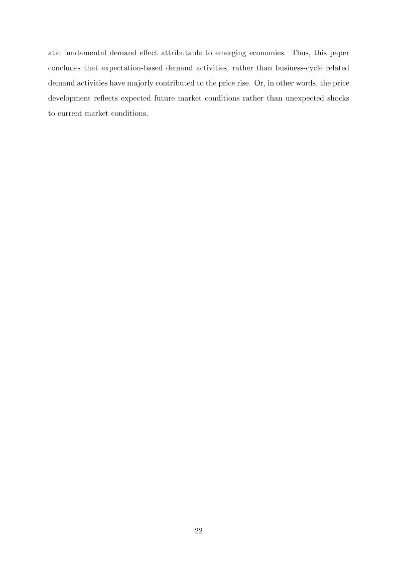
atic fundamental demand effect attributable to emerging economies. Thus, this paper

concludes that expectation-based demand activities, rather than business-cycle related

demand activities have majorly contributed to the price rise. Or, in other words, the price

development reflects expected future market conditions rather than unexpected shocks

to current market conditions.

22

5 Appendix

5.1 Re-Estimation of 3-Variables SVAR

We re-estimate Kilian (2009) for the sub-period of 2003-2010.22 The VAR model is based

on monthly data for

yt = (prodt, econactt, pricet)′

where prodt is the percentage change in global crude oil production, econactt refers to the

economic activity index and pricet is the real price of crude oil. The VAR representation

is

yt =9∑

i=1

Aiyt−i + et.23 (5)

The underlying SVAR allows to model the contemporaneous effects between the variables

yt:

A0yt =9∑

i=1

A∗i yt−i + εt (6)

with Ai = A−10 A∗i and et = A−10 εt. We impose the restriction matrix as in Kilian (2009)

as

et =

e∆prodt

eeconactt

epricet

=

a11 0 0a21 a22 0a31 a32 a33

εflow supply shockt

εflow demand shockt

εresidual shockt

(7)

As in Kilian (2009), we use monthly percentage changes of global crude oil production

taken from the Energy Information Administration (EIA) as measure of crude oil supply.

The refiner acquisition cost of imported crude oil, deflated by the US CPI, is used as

proxy for the real price of oil. While Kilian (2009) uses a self-composed shipping index

based on single cargo freight rates provided by Drewry’s, the follow-up paper by Kilian

and Murphy (2010) use the Baltic Dry Exchange Shipping index which is ”essentially

identical” (Kilian and Murphy, pg. 6) to the index used in Kilian (2009). As the latter

is readily available on data providing platforms, such as Datastream, we also use it here.

The shipping index appears to be non-stationary in levels and is thus investigated in

22For a more detailed description of the model see Section 2.23Note that we include only nine lags instead of 24 as in Kilian (2009). This is due to the shorter time

series used for the estimations.

23

growth rates.24 As in Kilian (2009), we use the the refiner acquisition cost of imported

crude oil, deflated by the US CPI, as proxy for the real price of oil. It is expressed in

logs. Our data start in February 2003 and range until February 2010.

Figure 7 displays the impulse response functions on the price of crude oil for the re-

estimated model of Kilian (2009).25 Neither a flow supply shock nor a flow demand shock

lead to a significant increase in the price of crude oil. We find significant effects in the

autoregressive part in the price of crude oil.

pri

ce

SVAR Impulse Response from prod


0 2 4 6 8 11 14 17

−0

.40

.00

.40

.8

pri

ce

SVAR Impulse Response from demand


0 2 4 6 8 11 14 17

−0

.05

0.0

00

.05

0.1

0

pri

ce

SVAR Impulse Response from price


0 2 4 6 8 11 14 17

−0

.05

0.0

50

.15

0.2

5


Figure 7: Impulse response function of the price for re-estimated Kilian Model

Figure 8 displays the historical decomposition of the crude oil price according to this

three-variable model. As to be expected from the impulse response functions, the main

driver of the price development seems to come from the residual which is interpreted as

precautionary demand in Kilian (2009). Neither cumulative effects from flow supply nor

from flow demand contribute in a visible way to the development of the crude oil price.

This result stands in contrast to Kilian (2009) and illustrates that the results are sensitive

24Note that Kilian (2009) uses a different operation in order to make the series stationary. The seriesis detrended and expressed in deviations from trend. Both manipulations yield the same results.

25The bootstrap-confidence-interval from price to price appears to be biased. According to Philipsand Spencer (2010) this bias is due to the bootstrap OLS estimate of the error covariance matrix in thereduced form VAR which is biased downwards.

24

to the selection of the sample period.


Time

2005 2006 2007 2008 2009 2010

−1.

00.

01.

0


Time

2005 2006 2007 2008 2009 2010

−1.

00.

01.

0


Time

2005 2006 2007 2008 2009 2010

−1.

00.

01.

0

Figure 8: Decomposition of crude oil price in three variables model

25

5.2 Re-Estimation of 3-Variables SVAR with OECD Produc-tion Indicator

pri

ce

SVAR Impulse Response from prod


0 2 4 6 8 11 14 17

−0

.50

.51

.01

.5

pri

ce

SVAR Impulse Response from demand


0 2 4 6 8 11 14 17

−0

.40

.00

.40

.8

pri

ce

SVAR Impulse Response from price


0 2 4 6 8 11 14 17

0.0

00

.05

0.1

0


Figure 9: Impulse response function of crude oil price with alternative aggregate demandmeasure

26


Time

2005 2006 2007 2008 2009 2010

−1.

00.

01.

0


Time

2005 2006 2007 2008 2009 2010

−1.

00.

01.

0


Time

2005 2006 2007 2008 2009 2010

−1.

00.

01.

0

Figure 10: Decomposition of Crude Oil Price with alternative aggregate demand measure

5.3 Test for Unit Roots

Table 3: Test for unit roots / stationarity tests

ADF test (k=4) ADF test (k=3) PP test KPPS testCrude oil price non stationary non stationary non stationary non stationaryCrude oil production stationary stationary stationary non stationaryShipping index non stationary non stationary non stationary non stationaryOECD production non stationary non stationary non stationary non stationaryMedia sentiment stationary stationary stationary non stationaryCLI non stationary* stationary non stationary non stationary

*stationary at 15 % levelADF test: Augmented Dickey-Fuller test, see Dickey and Fuller (1981)

PP test: Philips-Perron test, see Philips and Perron (1988)KPPS test: see Kwiatkowski et al. (1992)

27

5.4 Impulse Response Function of 4-Variable System

De

ma

nd



0 2 4 6 8 10 13 16

−0

.08

−0

.02

0.0

2

De

ma

nd



0 2 4 6 8 10 13 16

−0

.05

0.0

50

.10

De

ma

nd



0 2 4 6 8 10 13 16

−0

.01

0−

0.0

04

0.0

02

De

ma

nd



0 2 4 6 8 10 13 16

−0

.00

60

.00

00

.00

4


Figure 11: Impulse response function for supply

Su

pp

ly



0 2 4 6 8 10 13 16

−0

.10

0.0

00

.10

Su

pp

ly



0 2 4 6 8 10 13 16

−0

.08

−0

.04

0.0

00

.04

Su

pp

ly



0 2 4 6 8 10 13 16

−0

.00

40

.00

20

.00

6

Su

pp

ly



0 2 4 6 8 10 13 16

−0

.00

40

.00

00

.00

4


Figure 12: Impulse response function for demand

28

New

s



0 2 4 6 8 10 13 16

−3

−2

−1

01

2

New

s



0 2 4 6 8 10 13 16

−2

01

23

New

s



0 2 4 6 8 10 13 16

−0

.4−

0.2

0.0

0.2

New

s



0 2 4 6 8 10 13 16

−0

.3−

0.1

0.1


Figure 13: Impulse response function for news

5.5 Diagram of Fit

−0

.01

0.0

00

.01

0.0

2

Diagram of fit and residuals for Supply

0 20 40 60

−0

.01

00

.00

00

.00

50

.01

0

0 2 4 6 8 10 12

−0

.20

.41

.0

Lag

ACF Residuals

2 4 6 8 10 12

−0

.20

.00

.2

Lag

PACF Residuals

Figure 14: Diagram of fit and residual for supply

29

−0

.04

−0

.02

0.0

00

.01

Diagram of fit and residuals for Demand

0 20 40 60

−0

.00

50

.00

00

.00

5

0 2 4 6 8 10 12

−0

.20

.41

.0

Lag

ACF Residuals

2 4 6 8 10 12

−0

.20

.00

.2

Lag

PACF Residuals

Figure 15: Diagram of fit and residual for demand

5.5

6.0

6.5

7.0

7.5

Diagram of fit and residuals for News

0 20 40 60

−0

.4−

0.2

0.0

0.2

0.4

0 2 4 6 8 10 12

−0

.20

.41

.0

Lag

ACF Residuals

2 4 6 8 10 12

−0

.20

.00

.2

Lag

PACF Residuals

Figure 16: Diagram of fit and residual for news

30

4.0

4.5

5.0

5.5

Diagram of fit and residuals for Price

0 20 40 60

−0

.10

0.0

00

.05

0.1

0

0 2 4 6 8 10 12

−0

.20

.41

.0

Lag

ACF Residuals

2 4 6 8 10 12

−0

.20

.00

.2

Lag

PACF Residuals

Figure 17: Diagram of fit and residual for price

5.6 Correlations

31

Tab

le4:

Cor

rela

tion

sS

hip

pin

gin

dex

OE

CD

pro

dC

LI

Pet

r.co

ns

Net

sent

Cu

mu

l.se

nt

Oil

pri

ceS

hip

pin

gin

dex

1.0

00

-0.0

28

0.2

10

0.0

45

0.2

26*

-0.0

67

-0-0

52

OE

CD

pro

d-

1.0

00

0.6

48**

0.3

81**

0.1

95

0.7

65**

0.6

44**

CL

I-

-1.0

00

0.5

22**

0.5

31**

0.1

60

0.1

77

Pet

r.co

ns

--

-1.0

00

0.2

17*

-0-0

56

-0.2

56*

Net

sent

--

--

1.0

00

-0-0

31

0.0

86

Cu

mu

l.se

nt

--

--

-1.0

00

0.8

15**

Oil

pri

ce-

--

--

-1.0

00

32

6 References

Alquist, R.; Kilian, L. (2007). What Do We learn From the Price of Crude Oil Futures?

Journal of Applied Econometrics 25, 539-573.

Andrews DWK, Ploberger W (1994). Optimal Tests When a Nuisance Parameter is

Present Only Under the Alternative. Econometrica, 62, 1383-1414.

Bai J, Perron P (2003). Computation and Analysis of Multiple Structural Change Models.

Journal of Applied Econometrics, 18, 1-22.

Barsky, R.B.; Kilian, L.(2002). Do We Really Know that Oil Caused the Great Stagfla-

tion? A Monetary Alternative. In: NBER, Macroeconomic Annuals 2001 16, ed. Ben S.

Bernanke and Kenneth Rogoff, 27-83, Cambridge: MIT Press.

Bernanke, B. (1986). Alternative Explanations of the Money-Income Correlation. Carnegie-

Rochester Conference Series on Public Policy, Amsterdam: North-Holland.

Buyuksahin, B., Haigh, M.S., Harris, J.H., Overdahl, J.A., Robe, M.A. (2008). Funda-

mentals, trader activity and derivative pricing. EFA Bergen Meetings Paper. Available

at SSRN: ohttp://ssrn.com/abstract=9666924.

Breitung, J., Bruggemann, R., Lutkepohl, H. (2004). Structural Vector Autoregressive

Modeling and Impulse Responses. In: H. Lutkepohl, M. Kratzig (eds.), Applied Time

Series Econometrics. Chapter 4, pp. 159-196. Cambridge University Press. Cambridge.

Dickey, D.; Fuller, W. (1981). Likelihood Ratio Tests for Autoregressive Time Series with

a Unit Root. Econometrica 49, 1057-1072.

Engle, R.F. (1982). Autoregressive Conditional Heteroscedasticity with Estimates of the

Variance of United Kingdom Inflation. Econometrica, 50, 987-1007.

Fan, Y.; Xu, Y.F. (2011). What has driven oil prices since 2000? A structural change

perspective. Energy Economics 33 (6), 1082-1094.

Fry, R.; Pagan, A. (2009). Sign Restrictions in Structural Vector Autoregressions: A

Critical Review. NCER Working Paper 57.

33

Godfrey, L.G. (1978). Testing Against General Autoregressive and Moving Average Error

Models when the Regressors Include Lagged Dependent Variables. Econometrica, 46,

1293-1302.

Hamilton, J.D. (2003). What Is an Oil Shock? Journal of Econometrics 113(2), 363-398.

Hamilton, J.D. (2008). Understanding Crude Oil Prices. NBER Working Paper No.

14492.

Hamilton, J.D. (2009). Causes and consequences of the oil shock of 2007-2008.Brookings

Papers on Economic Activity, pp. 215-261.

Hamilton, J.D.; Herrera, A.M. (2004), Oil Shocks and Aggregate Macroeconomic Be-

havior: The Role of Monetary Policy. Journal of Money, Credit, and Banking 36, pp.

265-286.

Hamilton, J.D.; Wu, J.C. (2011). Risk Premia in Crude Oil Futures Prices. Working

Paper. University of California at San Diego.

Kaufmann, R.K. (2011). The role of market fundamentals and speculation in recent price

changes for crude oil. Energy Policy 39, 105-115.

Jarque, Carlos M.; Bera, Anil K. (1987). A Test for Normality of Observations and

Regression Residuals. International Statistical Review, 55 (2), 163-172.

Kilian, L (2009). Not all Oil Price Shocks are Alike: Disentangling Demand and Supply

Shocks in the Crude Oil Market. American Economic Review 99:3, 1053-1069.

Kilian, L.; Hicks, B. (2012). Did Unexpectedly Strong Economic Growth Cause the Oil

Price Shock of 2003-2008? forthcoming: Journal of Forecasting.

Kilian, L.; Murphy, D.P. (2011). The Role of Inventories and Speculative Trading in the

Global Market for Crude Oil. Forthcoming, Journal of the European Economic Associa-

tion.

Krugman, P. (2008). The Oil Nonbubble. Available at:

http : //www.nytimes.com/2008/05/12/opinion/12krugman.html

34

Kwiatkowski, D.; Philipps, P.C.B; Schmidt, P.; Shin, Y. (1992). Testing the Null Hy-

pothesis of Stationarity against the Alternative of a Unit Root. Journal of Econometrics

54, 159-178.

Lamla, M. J.; Sarferaz, S. (2012). Updating Inflation Expectations. KOF Working Paper

No. 301.

Lutkepohl, H. (2004). Vector Autoregressive and Vector Error Correction Models. In:

H. Lutkepohl, M. Kratzig (eds.), Applied Time Series Econometrics. Chapter 4, pp.

159-196. Cambridge University Press. Cambridge.

Muth, J. F. (1961): Rational Expectations and the Theory of Price Movements. Econo-

metrica , Vol. 29, No. 3 (Jul., 1961), pp. 315-335.

Pfaff, B. (2008). VAR, SVAR and SVEC Models: Implementation Within R Package

vars. Journal of Statistical Software, 27 (4).

Phillips, K. L.; Spencer, D. E. (2010): Bootstrapping Structural VARs: Avoiding a

Potential Bias in Confidence Intervals for Impulse Response Functions. MPRA Working

Paper.

Philipps, P.C.B; Perron, P. (1988). Trends and Random Walks in Macroeconomic Time

Series. Biometrika 75, 335-346.

R Development Core Team (2011). R: A Language and Environment for Statistical Com-

puting. R Foundation for Statistical Computing, Vienna, Austria. www.R-project.org

accessed 20.3.2011.

Sims, C.A. (1980). Macroeconomics and Reality. Econometrica 48(1), 1-48.

Singleton, K.J. (2011). Investor Flows and the 2008 Boom/Bust in Oil Prices. Working

paper. Stanford University.

Tang, K; Xiong, W. (2011). Index Investment and Financialization of Commodities.

Working Paper. Princeton University.

35

Documents

Moody Oil What is Driving the Crude Oil Price?