Monetary and Fiscal Policy Switching - Indiana …mypage.iu.edu/~eleeper/Papers/DavigLeeperChungJMCBFinal.pdf · HESS CHUNG TROY DAVIG ERIC M. LEEPER Monetary and Fiscal Policy Switching

HESS CHUNG

TROY DAVIG

ERIC M. LEEPER

Monetary and Fiscal Policy Switching

A growing body of evidence finds that policy reaction functions vary sub-stantially over different periods in the United States. This paper explores howmoving to an environment in which monetary and fiscal regimes evolve ac-cording to a Markov process can change the impacts of policy shocks. In oneregime monetary policy follows the Taylor principle and taxes rise stronglywith debt; in another regime the Taylor principle fails to hold and taxesare exogenous. An example shows that a unique bounded non-Ricardianequilibrium exists in this environment. A computational model illustratesthat because agents’ decision rules embed the probability that policies willchange in the future, monetary and tax shocks always produce wealth effects.When it is possible that fiscal policy will be unresponsive to debt at times,active monetary policy (like a Taylor rule) in one regime is not sufficientto insulate the economy against tax shocks in that regime and it can havethe unintended consequence of amplifying and propagating the aggregatedemand effects of tax shocks. The paper also considers the implications ofpolicy switching for two empirical issues.

JEL codes: E4, E5, E6Keywords: regime change, policy interactions, Taylor rule, fiscal theory of the price level.

TWO THEMES RUN through policy analysis: rules determiningpolicy choice are functions of economic conditions; those rules may change overtime. The themes reflect the views that actual policy behavior is purposeful, ratherthan arbitrary, and that good policy adapts to changes in the structure of the economyor to improvements in understanding how policy affects the economy.

We thank Michael Binder, Chuck Carlstrom, Betty Daniel, Behzad Diba, Jon Faust, Dale Henderson,Bartosz Mackowiak, Jim Nason, Giorgio Primiceri, Lars Svensson, Martin Uribe, Ken West, an anonymousreferee, and seminar participants at Banco de Portugal, Duke University, the Federal Reserve Bank ofCleveland, the Federal Reserve Board, and the ECB for helpful comments.

HESS CHUNG is a Ph. D. student at Indiana University (E-mail: [email protected]).TROY DAVIG is a Senior Economist at Federal Reserve Bank of Kansas City (E-mail:[email protected]). ERIC M. LEEPER is a Professor of Economics at Indiana University,Center for Applied Economics and Policy Research, and NBER (E-mail: [email protected]).

Received June 22, 2005; and accepted in revised form March 17, 2006.

Journal of Money, Credit and Banking, Vol. 39, No. 4 (June 2007)C© 2007 The Ohio State University

810 : MONEY, CREDIT AND BANKING

A growing body of evidence finds that policy reaction functions vary substantiallyover different periods in the United States. In light of this evidence of regime shifts,which is reviewed in Section 1, it is surprising that there is little formal modelingof environments where ongoing regime change is stochastic, and the objects sub-ject to change are parameters determining how the economy feeds back to policychoice.

This paper is the first step of a broader research agenda that explores how movingto environments in which monetary and fiscal regimes evolve according to a Markovprocess can change the impacts of and, more generally, the analysis of monetaryand fiscal policies.1 We consider interest rate rules for monetary policy and tax rulesfor fiscal policy; the rules switch stochastically between two regimes. In one regimemonetary policy follows the Taylor (1993) principle and taxes rise strongly withincreases in the real value of government debt; in another regime the Taylor principlefails to hold and taxes follow an exogenous stochastic process. Using convenientspecifications of policy rules, Section 2 presents an analytical example which showsthat a unique bounded equilibrium exists in this environment; in that equilibrium,lump-sum taxes always have wealth effects.

More standard forms of policy rules require that the model be solved numerically.Sections 3 and 4 lay out a conventional model of monetary–fiscal policy interac-tions and describe the computational methods used to solve the non-linear model.Section 5 derives the impacts of exogenous changes in monetary and tax policies ina regime-switching environment and contrast those impacts with their fixed-regimecounterparts. When regimes switch, agents’ decision rules embed the probability thatpolicies will change in the future and, in consequence, monetary and tax shocks al-ways produce wealth effects. Conventional fixed-regime analyses have found thatactive monetary policy (like a Taylor rule), which is designed to stabilize aggregatedemand and inflation, requires that fiscal policy adjust taxes in response to debt. Incontrast, when regimes change and it is possible that taxes will be unresponsive todebt at times, active monetary policy in one regime is not sufficient to insulate theeconomy against tax shocks in that regime, and may have the unintended consequenceof amplifying and propagating the aggregate demand effects of tax shocks.

It turns out that as long as private agents put probability mass on a regime inwhich taxes respond weakly (or not at all) to debt, lump-sum tax disturbances alwaysgenerate aggregate demand effects. Section 6 demonstrates this result by consideringa range of specifications for the stochastic process governing monetary–fiscal regime.

In Section 7 the paper considers the implications of policy switching for two empir-ical issues. First, the “price puzzle” that plagues monetary VARs is a natural outcomeof periods when monetary policy fails to obey the Taylor principle and taxes do not re-spond to the state of government indebtedness. Second, dynamic correlations betweenfiscal surpluses and government liabilities, which have been interpreted as consistentwith Ricardian equivalence, can be produced by an underlying equilibrium in whichtaxes matter.

1. Davig and Leeper (Forthcoming-a, Forthcoming-b) report other aspects of this agenda.

HESS CHUNG, TROY DAVIG, AND ERIC M. LEEPER : 811

Regime change is treated as exogenous throughout the paper. By helping withtractability and permitting more straightforward interpretations, this assumption is areasonable first step. It is also completely consistent with, for example, the massiveliterature on Taylor (1993) rules for monetary policy, which merely posits simplecharacterizations of policy behavior with exogenously chosen parameter values. It isworthwhile to examine whether exogenous regime change matters for the predictionsof standard models before tackling the more ambitious and arguably more plausiblesetup in which regime change is triggered by policy responses to the state of theeconomy.

A priori reasoning cannot determine whether and how much the paper’s resultsmight be affected by endogenizing regime change. Even when past change seemsclearly to be a response to economic conditions, such as President Carter’s appoint-ment of Paul Volcker as Fed chairman during the high inflation of 1979, the precisetiming and nature of the change are likely determined by non-economic considera-tions. Moreover, while some fiscal regime changes may be endogenous—the 1993tax hike after several years of large budget deficits—others may be driven largelyby political agenda—the 2002 and 2003 tax cuts in the face of rising expendituresand expanding government indebtedness. We approximate actual regime changes,which arise from a mix of endogenous and exogenous factors, by focussing entirelyon exogenous changes.

1. CONTACTS WITH THE LITERATURE

This paper makes contact with existing work in several areas. Sargent and Wallace(1981) were among the first to emphasize intertemporal aspects of monetary and fiscalpolicy interactions. With monetary and fiscal policy, there are two policy authoritiesthat jointly determine the price level and ensure the government is solvent. Whenone policy authority pursues its objective unconstrained by the behavior of the otherauthority, its behavior is “active,” whereas the constrained authority’s behavior is“passive.”2

If policy regime is fixed, active monetary policy coupled with passive fiscal policy—the policy mix implicit in the literature on the Taylor principle—produces conven-tional monetarist and Ricardian predictions of monetary and fiscal policy impacts.In contrast, when active fiscal policy combines with passive monetary policy—thecombination associated with the fiscal theory of the price level3—monetary and taxchanges generate wealth effects that shift aggregate demand, and policy impacts arenon-monetarist and non-Ricardian.

Lucas (1976) taught macroeconomists to think about policy changes in terms ofshifts in regime. But Lucas’s examples all involve once-and-for-all changes, rather

2. This follows Leeper’s (1991) taxonomy.3. See, for example, Leeper (1991), Sims (1994), Woodford (1995), and Cochrane (1998). Sims (1988)

is an important early contribution. See Leeper and Yun (2006) for a microeconomic exposition of the fiscaltheory in the presence of tax distortions.


than the ongoing process described in the history above. Cooley, LeRoy, and Raymon(1982, 1984), and Sims (1986, 1987) have argued that treating policy as makingonce-and-for-all choices is logically inconsistent. After all, if policy authorities cancontemplate changing regime, then regime is not permanent. If there has been a historyof changes in policy regimes, private agents will ascribe a probability distributionover those regimes. Agents’ expectations, and therefore their decision rules, willreflect their belief that policy changes are not once-and-for-all. This point resonatesespecially crisply in the United States, where the policy changes we aim to model areintrinsically temporary; they arose largely because of the personalities of the politicalplayers, rather than through the creation of new policy institutions or changes inexisting institutions’ legal mandates.

Clarida, Gali, and Gertler (2000, p. 149) argue that when the Fed failed to obeythe Taylor principle before 1979, it left “open the possibility of bursts of inflation andoutput that result from self-fulfilling changes in expectations.” The possibility of mul-tiple equilibria relies on the implicit assumption that fiscal policy was passive duringthis period. Woodford (1998b) suggests that fiscal policy may have been active dur-ing that period, implying that observed inflation emerged from a unique equilibrium.Favero and Monacelli (2003), Sala (2004), and Davig and Leeper (Forthcoming-a)offer empirical evidence that fiscal policy was active and monetary policy was passivein the 1960s and 1970s, supporting Woodford’s argument.

All this work is couched in terms of changes in policy regime, and there have beensome efforts to incorporate switching policy specifications into dynamic stochasticgeneral equilibrium models to study the fiscal theory of price level determination(FTPL) (Sims 1997, Woodford 1998a, Loyo 1999, Mackowiak 2006, Weil 2002, andDaniel 2003). But each of these papers considers only one-time changes in regime. Inaddition, Loyo (1999), Weil (2002), and Daniel (2003) consider only changes in fiscalregime, holding monetary policy behavior fixed. Given a history of both monetaryand fiscal regime switching, it is important to allow both policies to change. Thispaper generalizes the theoretical literature on monetary and fiscal policy interactionsby explicitly modeling regime change as an ongoing process. Both one-time changesin regime and changes in only fiscal or monetary policy behavior are special cases ofour specification.

There is work that models ongoing regime change (Andolfatto and Gomme 2003,Davig 2003, 2004, Leeper and Zha 2003, Schorfheide 2005, Andolfatto, Hendry, andMoran 2002). That work considers only exogenous processes for policy variables thatswitch regime. This paper makes substantive and technical contributions by extendingwork on ongoing regime change to allow the objects subject to change to be parametersthat determine how the economy feeds back to policy choice. This is the first exampleof which we are aware that allows for regime switching in parameters of endogenouspolicy rules in an equilibrium model, where the parameters determine existence anduniqueness.

Empirical findings that policy regimes have changed in important ways are diffi-cult to interpret without theory that models regime changes explicitly (Favero andMonacelli 2003, Sala 2004). This paper fills some of the theoretical holes.


Finally, the paper connects to two bodies of empirical work. It offers an interpre-tation of the price puzzle in monetary VARs that differs from the cost channel putforth by Barth and Ramey (2002) and Christiano, Eichenbaum, and Evans (2005).The paper also provides a counterexample to the empirical inferences drawn by Bohn(1998) and Canzoneri, Cumby, and Diba (2001) about the behavior of fiscal policy inthe United States.

1.1 A Quick Post–WW II History of Regimes Change

Many macroeconomists believe that U.S. monetary policy changed regimes in late1979. The view holds that monetary policy changed from a period where increases ininflation were passively accommodated to one where incipient inflation was activelycombatted with tighter policy.4 Taylor (1999a), Clarida, Gali, and Gertler (2000), andLubik and Schorfheide (2004), among others, found that from 1960 to 1979 the Fedfollowed an interest rate rule that responded only weakly to inflation, failing to satisfythe Taylor principle. Since the early 1980s, the Taylor principle has been satisfied,according to this empirical work. But even the most sanguine observers of recent Fedsuccesses cannot exclude the possibility of a return to the days when monetary policyaccommodated inflation, as in Sargent’s (1999) analysis of American inflation.

Less well appreciated is the fact that fiscal policy may also have experiencedchanges in regime.5 In some periods, taxes are adjusted passively in response tochanging debt levels; at other times, tax changes are active attempts to achieve non-budgetary macroeconomic goals.

The history of tax policy illustrates the pendulum swings in policy. In the 1950staxes were increased three times on the grounds of budget balancing, in large partto finance the Korean War (Ohanian 1997). By the 1960s, with the rise of the “neweconomics,” tax changes were initiated primarily as a countercyclical tool (Heller1967). Budget balance had slipped into the background of tax debates. This trendcontinued for two decades. The resulting explosion in Federal government debt andits associated interest payments shifted priorities once again toward budget balancing,and eventually in the 1980s and 1990s, Presidents Reagan, Bush, and Clinton all signedlegislation that raised taxes to reduce budget deficits. By the time the tax cut of 2001was ratified by Congress, the rationale had shifted from budget concerns to economicstimulus. Both of the last two tax reductions—2002 and 2003—were unambiguouslymotivated by countercyclical objectives. Evidently over the past 50 years fiscal policybehavior has fluctuated between periods when taxes were adjusted in response to thestate of government indebtedness and those when other priorities drove tax decisions.

4. Sargent (1999) and Cogley and Sargent (2002, 2005) are consistent with this view. There is notuniversal acceptance of the view that policy rules have changed in important ways over the post–WorldWar II period. For example, Bernanke and Mihov (1998), Sims (1998), Hanson (2006), and Sims and Zha(2006) conclude that while monetary policy shocks exhibit heteroskedasticity, the endogenous response ofpolicy to the economy is best described by constant parameters.

5. For details see Pechman (1987), Poterba (1994), Stein (1996), Steuerle (2002), and Yang (Forth-coming).


That both monetary and fiscal regimes have fluctuated is confirmed by Faveroand Monacelli (2003) and Davig and Leeper (Forthcoming-a), who explicitly modelregime switching in their estimates of monetary and tax policy rules in the UnitedStates. Taylor (1996, 2000) and Auerbach (2002) document changes in the respon-siveness of taxes to macro conditions, providing further evidence that tax policy ruleschanged.

Against this history of shifts in policy rules, we use very simple models to take stepstoward examining the implications of the kinds of regime changes that the UnitedStates has actually experienced. Although stark, the models highlight that regimeswitching generates mechanisms that will continue to be present in richer modelswhere the mechanisms are harder to isolate.

2. AN ANALYTICAL EXAMPLE WITH REGIME SWITCHING

Canzoneri, Cumby, and Diba (2001) (CCD) argue that Ricardian equilibria are, ina certain sense, more general than non-Ricardian equilibria. They make this argumentby proving a proposition that states that over time the response of the governmentsurplus to total government liabilities merely needs to be bounded away from zeroinfinitely often for there to exist equilibria that exhibit Ricardian equivalence. Thekey point is that the private sector must expect taxes to adjust “sooner or later,”though the adjustment can be arbitrarily small and infrequent. Because the propositiondoes not require the fiscal response to be strong enough to make the evolution ofgovernment debt stable, the Ricardian equilibria CCD consider are potentially oneswith an unbounded debt–output ratio.

Equilibria with unbounded debt–output ratios may not be the most interesting orrelevant ones to consider. And they may be misleading if the impacts of taxes hinge onthe unboundedness assumption. Unbounded debt–output ratios are well outside anycountry’s experience, so it is impossible to tell if policy authorities would permit suchequilibria to occur. It is quite possible that if a country’s policies made its debt–outputratio appear to grow without limit, the country would undergo fundamental macropolicy reforms of the type that neither we nor CCD consider. We restrict attention toequilibria in which the debt–output ratio is bounded.

This section presents an analytical example in which policies that satisfy theassumptions of CCD’s proposition deliver a non-Ricardian equilibrium that is uniquewithin the set of equilibria with bounded debt–output ratios. Important conclusionsappear to hinge on CCD’s assumption of unboundedness.

Consider a constant endowment version of Sidrauski (1967), modified to includean interest rate rule for monetary policy and a tax rule for fiscal policy. If governmentconsumption is constant, then in equilibrium the representative agent’s consumption,c, is also constant, as is the real interest rate. Preferences over consumption and realmoney balances are logarithmic. This model implies a Fisher equation

1/Rt = βEt (1/πt+1) , (1)


where 0 < β < 1 is the discount factor, Rt is the gross nominal interest rate on one-period nominal government debt, π t+1 is the gross inflation rate between t and t + 1,and the expectation is taken with respect to a set �t that contains information datedt and earlier, including the history of regimes up to t . The money demand function is

mt = Rt

Rt − 1c, (2)

where mt = Mt/Pt is the real value of money balances.Monetary policy adjusts the nominal interest rate in response to inflation according

to the rule

Rt = exp [α0 + α(St )πt + θt ] , (3)

where πt ≡ ln πt , θt is an i.i.d. shock, St is the current regime, and α(St) is a regime-dependent parameter. Tax policy follows a rule that adjusts lump-sum taxes in responseto the real value of total government liabilities:

τt = γ0 + γ (St )(bt−1 + mt−1) + ψt , (4)

where τ t is the level of lump-sum taxes, bt−1 = Bt−1/P t−1 and mt−1 are the real valuesof debt and money at the beginning of period t , and ψ t is an i.i.d. disturbance. Theresponse of taxes to liabilities takes on values that depend on the realization of regime.St obeys an N-state Markov chain with transition probabilities P [St = j |St−1 = i] =pi j , where i , j ∈ {1, N}.

The government’s flow budget identity holds at each date t ≥ 0:

Bt + Mt

Pt+ τt = g + Mt−1 + Rt−1 Bt−1

Pt, (5)

given initial nominal liabilities M −1 + R−1 B−1 > 0.Define the expectation error

ηt+1 ≡Rt

πt+1

Et

(Rt

πt+1

) = βRt

πt+1, (6)

where the equality comes from using the Fisher equation. Combining (1) and (3) andusing (6), the inflation process obeys

πt+1 = α(St )πt + α0 + θt − ηt+1 + ln β. (7)

Let lt = bt + mt . Equations (4) and (5) together with (2) imply that governmentliabilities evolve according to

lt =[

Rt−1

πt− γ (St )

]lt−1 − Rt−1

πtc + D − ψt , (8)

where D = g − γ 0 .


Assume that (i) Et (γt+1) = γ ; (ii) γ satisfies |1/β − γ | > 1; (iii) the inflationprocess given by (7) is stable in expectation (that is, there exists a 0 < ξ < ∞ suchthat |Etπt+k | < ξ for all k). Assumptions (i) and (ii) mean that on average fiscal policyis active and assumption (iii) means that on average monetary policy is passive (theTaylor principle does not hold on average).6

Iterate forward on (8) to obtain (for k ≥ 0)

lt+k =k∏

j=0

(Rt−1+ j

πt+ j− γt+ j

)lt−1

+k∑

j=0

k− j∏i=1

(Rt−1+i+ j

πt+i+ j− γt+i+ j

) (D + Rt−1+ j

πt+ jc − ψt+ j

). (9)

To solve (9), take expectations as of t − 1, apply the law of iterated expectations,and use the Fisher equation. Then we can replace the terms Rt−1+ j

πt+ jwith 1

β. Under the

assumption that Et [γ t+1] = γ , (9) becomes

Et−1 (lt+k) = (1/β − γ )k+1

[lt−1 − c

(1/β − D/c

1/β − γ − 1

)]+ c

(1/β − D/c

1/β − γ − 1

). (10)

Stability requires that lt−1 = c( 1/β−D/c1/β−γ−1 ), which is positive if D/c < 1/β. The value

of η t is obtained from the budget constraint after substituting in the value of l:

ηt = β(1 + γ (St )) (1/β − D/c) − (D/c) (1/β − γ − 1)

1 + γ − D/c

+ β

c

(1/β − γ − 1

1 + γ − D/c

)ψt . (11)

Equation (11) is the unique equilibrium mapping from the tax disturbance, ψ t , andthe realization of the tax feedback parameter, γ (St), to the forecast error in inflation.The solution for η and the stable inflation process (7) uniquely determine inflation.For an equilibrium of this type to exist, we restrict the parameters to assure that η t ,which is the ratio of two positive numbers, is positive for any realization of ψ t . Asufficiently small value for D/c, coupled with a sufficiently high bounded negativesupport for ψ will do the job.

As a concrete example, suppose there are two regimes, N = 2, and that the policyparameters take on the values

α(St ) ={

α(1) for St = 1α(2) for St = 2

γ (St ) ={

γ (1) for St = 1γ (2) for St = 2

.

6. Davig, Leeper, and Chung (2004) derive the stability conditions for the inflation process.


Further suppose that α(1) and α(2) are sufficiently small such that, given the transitionprobabilities, the inflation process (7) is stable in expectation. The assumption thatthe tax parameters have constant mean implies

E[γt+ j |St = 1, �t ] = γ (1)p11 + γ (2)p12

= E[γt+ j |St = 2, �t ] = γ (1)p21 + γ (2)p22 ≡ γ,(12)

j > 0. By assumption |β−1 − γ | > 1. If either γ (1) or γ (2) is positive and jointlythey satisfy (12), then the model satisfies CCD’s premise that taxes adjust to debtinfinitely often. But as (11) makes clear, negative tax disturbances generate wealtheffects that raise the inflation rate. The only equilibrium with bounded debt is one inwhich Ricardian equivalence breaks down.

This does not deny the existence of Ricardian equilibria of the kind that CCDemphasize. But if those equilibria do exist, they must imply debt–output ratios thatgrow without bound.

3. A COMPUTATIONAL MODEL

We turn now to a variant on the model in Section 2, which is less convenientanalytically but more closely tied to actual policy behavior. Because the variant doesnot admit an analytical solution, we use Coleman’s (1991) monotone map method tofind a fixed point in the economy’s decision rules.

3.1 Households

As before, the representative consumer receives a constant endowment each period,yt = y, of which a constant gt = g < y is consumed by the government. Agents chooseconsumption, ct, and decide how to allocate portfolio holdings between values ofmoney, mt = Mt/Pt, and bonds, bt = Bt/Pt. The household’s problem is

max E0

∞∑t=0

β t [log(ct ) + δ log(mt )], (13)

subject to

ct + mt + bt + τt = y + mt−1

πt+ Rt−1

bt−1

πt, (14)

where δ > 0. The household takes initial nominal assets as given: M −1 + R−1 B−1

> 0. Expectations at date t are taken with respect to �t . Policy is the sole source ofuncertainty.

In equilibrium, ct = c = y − g and the first-order necessary conditions reduce tothe Fisher equation (1) and the money demand relation

mt = δc

(Rt

Rt − 1

). (15)


The optimal paths for real balances and bonds must also satisfy their respectivetransversality conditions.

3.2 Policy Specification

The policy specifications in the computational model connect to the existing liter-ature and actual policy behavior. The monetary and tax rules are

Rt = α0(St ) + α1(St )πt + θt , (16)

τt = γ0(St ) + γ1(St )bt−1 + ψt , (17)

where St ∈ {1, 2} , θt ∼ IDN(0, σ 2θ ), and ψ t ∼ IDN(0, σ 2

ψ ). The reaction coefficientstake values that depend on regime:

αi (St ) ={αi (1) for St = 1αi (2) for St = 2

, γi (St ) ={γi (1) for St = 1γi (2) for St = 2

, for i = {0, 1} ,

In this economy with perpetually full employment, an interest rate rule for mon-etary policy is clearly not optimal. If anything, it will reduce private welfare. Weemploy (16) for two reasons. First, it closely resembles monetary policy rules thathave received detailed study in recent years (Taylor 1999b). Second, (16) producesfeatures of an equilibrium that will continue to hold in models with frictions in whichrules from the general class to which (16) belongs are optimal. Fiscal rules like (17)that make taxes respond to debt (rather than total liabilities, as in (4)) are widely usedin model simulations (Bryant, Hooper, and Mann 1993), analytical studies of mon-etary and fiscal policy interactions (Leeper 1991, Sims 1997), and empirical work(Favero and Monacelli 2003). Specification (4) has the conceptually appealing fea-ture that it separates monetary and fiscal policy: an open-market operation that hasoffsetting effects on m and b does not affect taxes under (4), while it does under(17). Specification (17), however, has the realistic feature that fiscal authorities re-spond to the state of government debt, rather than the sum of debt and high-poweredmoney.

The government uses a combination of lump-sum taxes, new one-period nominalbonds and money creation to finance government purchases and debt payments andsatisfy the government’s flow budget identity (5).

In a fixed-regime version of this model, Leeper (1991) shows that the existenceand uniqueness of equilibrium depend on the policy feedback parameters. In a lin-ear approximation to the model, a monetary authority that reacts aggressively toinflation, |α1β| > 1 combined with a fiscal authority that raises taxes sufficientlyto cover interest payments and principle on the debt, |β−1 − γ1| < 1, imply a lo-cally unique stationary equilibrium consistent with Ricardian equivalence. This pol-icy combination is referred to as active monetary and passive fiscal policy (AM/PF).7

7. Logarithmic preferences make money essential and eliminate Obstfeld and Rogoff’s (1983) spec-ulative hyperinflations as potential equilibria. This allows the Taylor principle, coupled with passive tax


A monetary authority that reacts weakly to inflation, |α1β| < 1, together with a fis-cal authority that reacts weakly to real debt, |β−1 − γ1| > 1, imply a locally uniquestationary equilibrium where the path of taxes affects the inflation rate. This policycombination is referred to as passive monetary and active fiscal policy (PM/AF).One version of the fiscal theory of the price level emerges as the special case α1 =γ 1 = 0.

We use the local results from the linearized (fixed-regime) model to guide parameterchoices for the non-linear switching model. For most of this paper regime 1 combinesactive monetary policy with passive fiscal policy (AM/PF): |α1(1)β| > 1 and |β−1 −γ1(1)| < 1. Regime 2 combines passive monetary policy with active fiscal policy(PM/AF): |α1(2)β| < 1 and

∣∣β−1 − γ1(2)∣∣ > 1.8

Regimes follow a two-state Markov chain governed by the transition matrix

=(

p11 p12

p21 p22

), (18)

where pi j = P [St = j |St−1 = i] = pi j , i, j = 1, 2, and p12 ≡ 1 − p11 and p21 ≡ 1− p22.9

We assume agents observe current and past realizations of regimes and of exogenousdisturbances.

3.3 Competitive Equilibrium

The bounded equilibrium for the economy with regime-switching policy rules isdefined as:

Given the state vector �t = {wt−1, bt−1, θt , ψt , St }, where w t−1 = Rt−1 bt−1 +mt−1, a bounded competitive equilibrium for the economy consists of a continu-ous decision rule for real debt, bt = hb (�t ) , and a continuous pricing function,πt = hπ (�t ) , such that: (i) taking sequences {Rt , τt , πt , θt , ψt , St } as given, the rep-resentative agent’s optimization problem is solved; (ii) the fiscal authority sets τ t

according to (17) and the monetary authority sets Rt according to (16); (iii) the gov-ernment budget identity (5) and the aggregate resource constraint, yt = ct + g, aresatisfied.

policy, to deliver uniqueness. As Sims (1997) shows, if money is inessential, this policy mix does notproduce a determinant equilibrium.

8. The model is specified to ensure that the problems arising from multiple steady-state equilibria,which Benhabib, Schmitt-Grohe, and Uribe (2001a, 2001b, 2002) emphasize, cannot occur.

9. Although our reading of macro policy history and Favero and Monacelli’s (2003) and Davig andLeeper’s (Forthcoming-a) estimates suggest that monetary and fiscal policy have not switched syn-chronously, as a first step we assume that they do. Full non-synchronous switching would allow theeconomy to evolve for a time under policies that are both passive. A PM/PF mix, if it were expected to lastforever, yields indeterminacy of equilibrium. See Davig and Leeper (Forthcoming-a) for details.


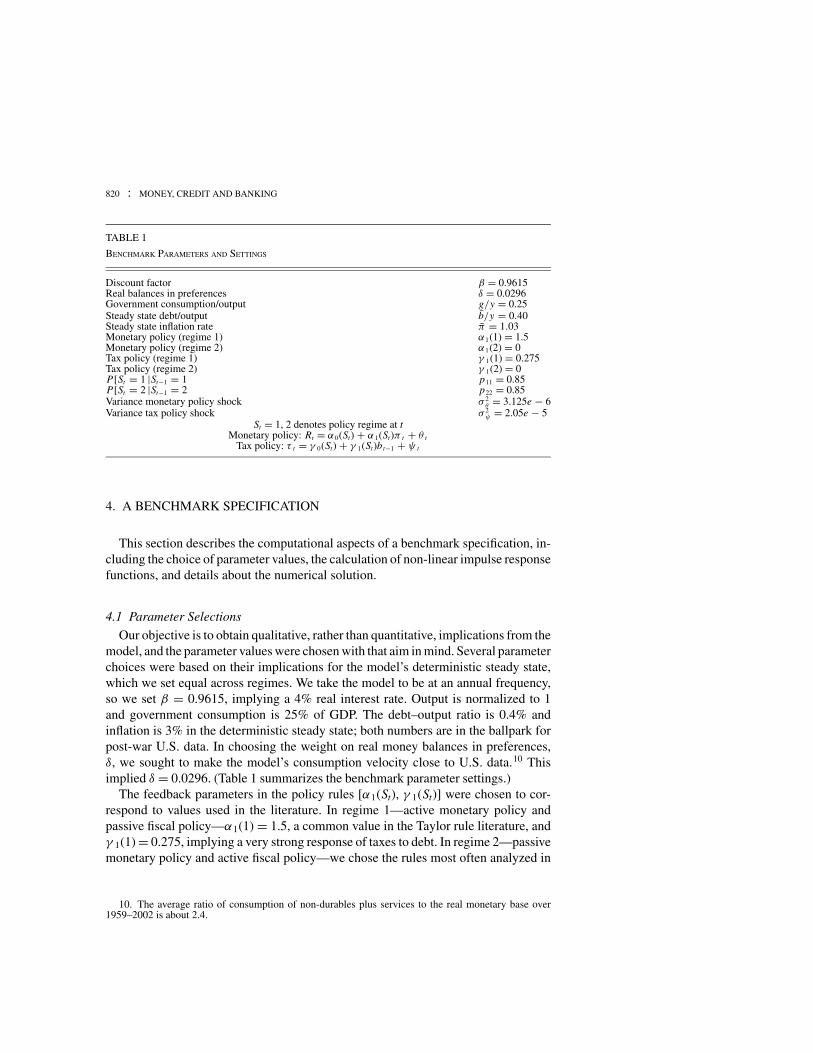
TABLE 1

BENCHMARK PARAMETERS AND SETTINGS

Discount factor β = 0.9615Real balances in preferences δ = 0.0296Government consumption/output g/y = 0.25Steady state debt/output b/y = 0.40Steady state inflation rate π = 1.03Monetary policy (regime 1) α1(1) = 1.5Monetary policy (regime 2) α1(2) = 0Tax policy (regime 1) γ 1(1) = 0.275Tax policy (regime 2) γ 1(2) = 0P[St = 1 |St−1 = 1 p11 = 0.85P[St = 2 |St−1 = 2 p22 = 0.85Variance monetary policy shock σ 2

θ = 3.125e − 6Variance tax policy shock σ 2

ψ = 2.05e − 5St = 1, 2 denotes policy regime at t

Monetary policy: Rt = α0(St) + α1(St)π t + θ tTax policy: τ t = γ 0(St) + γ 1(St)bt−1 + ψ t

4. A BENCHMARK SPECIFICATION

This section describes the computational aspects of a benchmark specification, in-cluding the choice of parameter values, the calculation of non-linear impulse responsefunctions, and details about the numerical solution.

4.1 Parameter Selections

Our objective is to obtain qualitative, rather than quantitative, implications from themodel, and the parameter values were chosen with that aim in mind. Several parameterchoices were based on their implications for the model’s deterministic steady state,which we set equal across regimes. We take the model to be at an annual frequency,so we set β = 0.9615, implying a 4% real interest rate. Output is normalized to 1and government consumption is 25% of GDP. The debt–output ratio is 0.4% andinflation is 3% in the deterministic steady state; both numbers are in the ballpark forpost-war U.S. data. In choosing the weight on real money balances in preferences,δ, we sought to make the model’s consumption velocity close to U.S. data.10 Thisimplied δ = 0.0296. (Table 1 summarizes the benchmark parameter settings.)

The feedback parameters in the policy rules [α1(St), γ 1(St)] were chosen to cor-respond to values used in the literature. In regime 1—active monetary policy andpassive fiscal policy—α1(1) = 1.5, a common value in the Taylor rule literature, andγ 1(1) = 0.275, implying a very strong response of taxes to debt. In regime 2—passivemonetary policy and active fiscal policy—we chose the rules most often analyzed in

10. The average ratio of consumption of non-durables plus services to the real monetary base over1959–2002 is about 2.4.


the FTPL literature: α1(2) = 0 and γ 1(2) = 0, making both the nominal interest rateand taxes exogenous.

Given the settings for [α1(St), γ 1(St)] and the assumptions on the deterministicsteady-state values for debt and inflation, the intercept terms for the policy rules[α0(St), γ 0(St)] are determined.

For the benchmark specification, we make the transition probabilities betweenregimes equal, with the regimes only moderately persistent. With p11 = p22 = 0.85,the average regime duration is 6 2

3 years. This duration is briefer than seems realistic,but it makes the differences between regimes clear.11

The variances of the i.i.d. policy shocks, (θ t , ψ t ), are fixed across regimes. We setσ 2

θ = 3.125e − 6 and σ 2ψ = 2.05e − 5. A constant σ 2

ψ implies the same-sized taxshock in each regime: two standard deviations amount to a change in taxes relative toits stationary mean of about 3 1

2 %. Because of simultaneity between Rt and π t in themonetary policy rule, a constant σ 2

θ can imply very different changes in the nominalinterest rate from a given shock: a two standard deviation shock to θ t lowers Rt 5basis points in regime 1, and 35 basis points in regime 2.

4.2 Non-Linear Impulse Response Analysis

The methods of Gallant, Rossi, and Tauchen (1993) are used to assess the dynamicimpacts of shocks to fiscal and monetary policy. Impulse response functions reporthow a shock makes the paths of variables differ from their baseline paths. We takethe baseline to be the regime-dependent steady state, which is defined as a regime-dependent steady state, {π ( j), b ( j)}, is a value for the state vector, �, such that

| [πt , bt ]′ | − | [πt−1, bt−1]′ | < ε,

for ε > 0 and St−1 = St = j , where j = {1, 2} .

For example, the impact effect of an i.i.d. shock to lump-sum taxes on inflation,conditioning on an AM/PF policy (regime 1), is described by

πt = hπ(w, b, 0, ψt , 1

) − hπ (�), (19)

where hπ (�) is the regime-dependent steady-state value for inflation. The paths forinflation and debt are then recursively updated, holding regime constant. Althoughconditioning on an unchanged regime is obviously counterfactual, if the regime isnot an absorbing state, this definition of an impulse response function allows us tomake more direct comparisons to fixed-regime models. The analysis that follows usesderivations analogous to (19) to trace out the impacts of perturbing one shock, holdingall other sources of randomness fixed.

11. In Section 6 we examine the equilibrium’s sensitivity to variation in policy settings, includingfeedback parameters and regime duration.


4.3 Average versus Marginal Sources of Financing

This paper follows Sargent and Wallace (1981) by emphasizing the fiscal financingconsequences of alternative monetary and tax policy rules. We wish to highlight adistinction that does not appear in Sargent and Wallace: there can be an importantdifference between the average and the marginal source of financing.12 In the model’sdeterministic steady state direct taxation through τ constitutes over 96% of totalrevenues, leaving seigniorage to cover a little over 3%. Although the means of thestochastic steady states across regimes differ slightly from the deterministic steadystate values, the message is the same: on average seigniorage is a trivial source of fiscalfinancing. In regime 1 (AM/PF), seigniorage averages about 3.6% of total revenues(0.99% of output), and in regime 2 it averages 3.4% (0.95% of output). These numbersare consistent with the U.S. evidence that King (1995) cites.

There are three distinct marginal sources of financing that exogenous disturbancesmay generate. The first arises from an instantaneous jump in the price level thatrevalues existing nominal government liabilities. The other two sources are dynamic,arising from changes in the present values of the primary surplus and seigniorage.Define the present value at date t of the primary surplus from date t + 1 onward as

xt =∞∑

s=0

[(s∏

j=0

πt+ j+1 R−1t+ j

)(τt+s+1 − g)

](20)

and of seigniorage as

zt =∞∑

s=0

[(s∏

j=0

πt+ j+1 R−1t+ j

) (mt+s+1 − mt+sπ

−1t+s

)]. (21)

The government’s present value budget identity implies

Bt

Pt= xt + zt . (22)

After taking expectations at date t of both sides of (22), Cochrane (2005) refers tothis relationship as a “debt valuation equation,” which he uses to exposit the FTPL.When expected xt and zt are fixed by policy behavior, a bond-financed tax cut mustmake Pt jump to ensure the equilibrium value of debt does not change. This is theinstantaneous marginal source of financing.

12. This distinction is sometimes overlooked. King and Plosser (1985), for example, point to the factthat averaged across time inflation financing is a trivial source of revenues in the United States as suggestingthat inflation taxes should also be inconsequential in response to various shocks to the economy. In addition,many observers dispute the relevance of the dynamic policy interactions that Sargent and Wallace describeon the grounds that most developed countries do not rely heavily on seigniorage revenues (King 1995).Castro, Resende, and Ruge-Murcia (2003) draw a similar conclusion for OECD countries. See Grilli (1989),Cohen and Wyplosz (1989), and Centre for Economic Policy Research (1991) for related discussions inthe context of European Monetary Union.


Under different policy assumptions, exogenous shocks may bring forth expectedchanges in xt or zt. Given the benchmark parameters, when regimes are permanent,i.i.d. shocks to taxes and to monetary policy generate no change in the present valueof seigniorage in regime 1 (AM/PF), though they do affect the present value ofsurpluses. Tax shocks in regime 2 (PM/AF) leave both xt and zt unchanged, whilemonetary policy shocks change both xt and zt. In contrast, in the switching model onlytax disturbances in regime 2 leave the present values in (20) and (21) unchanged.13

4.4 Computational Details

It may seem natural to solve the model by first linearizing around the regime-dependent steady states. But in the switching model, policy parameters as well aspolicy shocks are random variables. For some policies of interest, it can turn out thatthe one-step-ahead forecast error in inflation from the Fisher relation is correlated withfuture policy parameters. Linear methods can fail to capture this correlation, leadingthe approximations to incorrectly classify existence and uniqueness of equilibrium.Appendices in Davig, Leeper, and Chung (2004) show this in detail for two differentlinearization methods.

The complete model consists of the first-order necessary conditions from therepresentative agent’s optimization problem, constraints, specification of the policyprocess, and the transversality conditions on real balances and bonds. The solutionmethod, based on Coleman (1991), conjectures candidate decision rules that reducethe system to a set of non-linear expectational first-order difference equations. Thesolution consists of two functions that map the current state into values for real debtand inflation.

The decision rule for real debt, hb(�t ), and the pricing function for inflation,hπ (�t ), are found by substituting the conjectured rules into the complete model,represented by

Rt = α0(St ) + α1(St )hπ (�t ) + θt (23)

τt = γ0(St ) + γ1(St )bt−1 + ψt (24)

mt = δc

[Rt

Rt − 1

](25)

R−1t = β{Et [h

π (�t+1)]}−1 (26)

hb (�t ) + mt + τt = g + wt−1 (hπ (�t ))−1

, (27)

where the future state, �t+1, is

�t+1 = {wt , bt , θt+1, ψt+1, St+1} ,

and wt = Rtbt + mt.

13. If regime 2 set γ 1(2) > 0 but small and 0 < α1(2) < 1, both present values would change.


Substituting (23)–(25) into (26) and (27) and using numerical quadrature to eval-uate the triple integrals representing expected inflation reduce the system to twoequations in the unknown functions hb and hπ . The system is solved for every set ofstate variables defined over a discrete partition of the state space, yielding updatedapproximations to hπ (�t ) and hb(�t ) at every node in the state space. When evaluat-ing the integral, non-linear interpolation is used to compute function values for statesthat lie off the discretized state grid. This procedure is repeated until iterations updatethe current decision rules by less than some ε > 0 (set to 1e − 12).

The solution is verified using three criteria. First, residuals for the governmentbudget identity and first-order conditions must be close to zero on each node of thestate space. Second, we check that the government’s present value budget identity(22) holds to some tolerance. Third, the unconditional mean of expectational errorsmust be approximately zero in random simulations. We verify sufficient conditionsby observing the solution implies stationary paths for real debt and real balances. Thesolution is verified to be locally unique by randomly perturbing the converged ruleand checking that it converges back to the initial rule. Across discrete nodes in thestate space, the largest residual is 2e − 15. The convergence criterion was satisfied ateach node.

5. COMPUTATIONAL RESULTS

This section describes results from the benchmark specification and contrasts thoseresults with predictions from the model with fixed policy regime.

5.1 Impacts of Policy Shocks in Regime 1 (AM/FP)

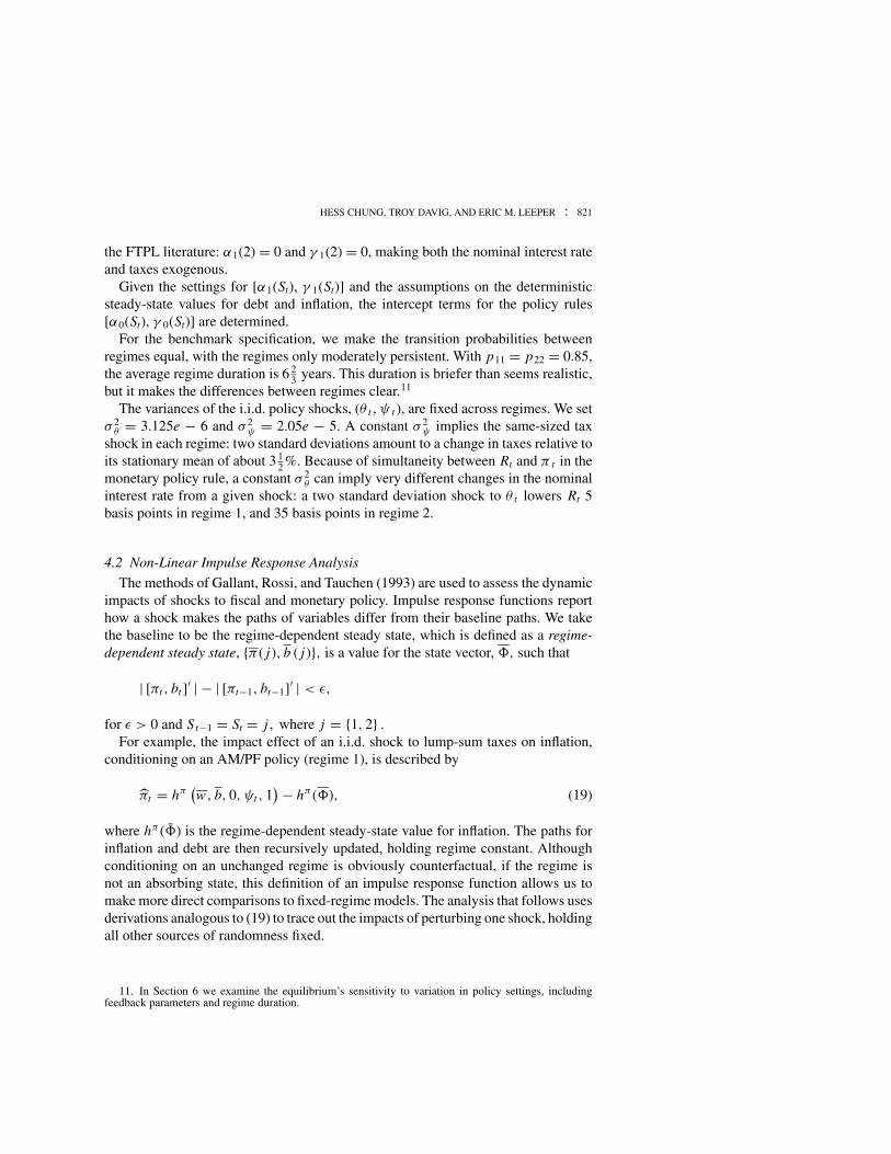
The impacts of monetary and fiscal policy shocks are reported in Figures 1 (con-ditioning on remaining in regime 1) and 3 (conditioning on remaining in regime 2),computed as described in Section 4.2; solid lines are responses to a one-time i.i.d. taxcut and dashed lines are responses to a one-time i.i.d. monetary easing.

Tax shocks. In regime 1, fiscal policy would exhibit Ricardian equivalence if policyregime were expected to last forever. A bond-financed tax cut brings forth an expec-tation of future taxes whose present value exactly equals the increase in the value ofdebt. With no change in net wealth, demand for goods is unchanged at initial pricesand interest rates. Unchanged inflation implies unchanged nominal rates, leaving thepresent value of seigniorage also unchanged.14

When regime can change, agents initially treat a tax cut as an increase in wealth.Because they place positive probability on switching to regime 2 (PM/AF), wheretaxes are exogenous, the current tax reduction exceeds the expected present valueof tax increases in the future. A switch to regime 2 with fixed taxes brings with it a

14. Leeper (1993) reports responses to monetary and tax policy shocks for a closely related fixed-regimemodel under regimes 1 and 2.


0 5 10 152.8

2.9

3

3.1

3.2

π

ψθ

0 5 10 150.35

0.36

0.37

0.38

0.39

b

0 5 10 156.8

6.9

7

7.1

7.2

7.3

R

0 5 10 150.235

0.24

0.245

0.25

0.255

τ

0 5 10 15

0

2

4

6

M g

row

th

0 5 10 150

2

4

6

8

10

B g

row

th

0 5 10 150.125

0.13

0.135

0.14

0.145

PV

sur

plus

0 5 10 150.225

0.23

0.235

0.24

PV

sei

gnio

rage

FIG. 1. Impacts of Policy Shocks Conditional on Regime 1 (AM/FP).

NOTE: For the tax shock, ψ , the figure plots deviations of E[xt+ j |{St+ j = 1, ψt < 0, θt = 0, j ≥ 0}] from steady stateand for the monetary policy shock, θ , the figure plots analogous deviations of E[xt+ j |{St+ j = 1, ψt = 0, θt < 0, j ≥ 0}].Because the shocks are i.i.d., their expected future values are zero.

discrete devaluation of government debt through an increase in the price level. At theinitial price level, agents perceive that their wealth has risen and they attempt to raise


their consumption profile. This increases aggregate demand and the current inflationrate in this economy with a fixed supply of goods (Figure 1).

With α1(1) = 1.5 in regime 1, monetary policy reacts to the higher inflation rate byraising the nominal interest rate. This creates an expectation that inflation will remainabove its stationary level in regime 1, which is consistent with the anticipated debtdevaluation. When the impulse response functions are conditioned on the economyremaining in regime 1, active monetary policy propagates the transitory tax cut,generating persistently higher inflation and nominal rates. The persistence is so strongthat variables remain away from their pre-shock levels over 10 periods after the taxcut.

In periods following the tax cut, taxes increase, because in regime 1 policy passivelyraises taxes when debt increases. But the rise in the value of debt exceeds the presentvalue of these tax increases, with the difference made up by an increase in the presentvalue of inflation taxes.

Inflation exhibits stable responses to policy shocks, as Figure 1 shows. Based onintuition derived from single-equation linearized models, this outcome may seemcounterintuitive. Conditional on staying in a regime with active monetary policy, inlinearized models the Taylor principle makes the inflation equation unstable: afteran i.i.d. policy shock, inflation jumps immediately to offset the effect of the policyshock on expected inflation; in the next period, inflation jumps back to its steady-statevalue. In the non-linear computational results, by contrast, the response of inflationis serially correlated. Moreover, one might think that, since we have a fiscal theoryequilibrium, the surprise revaluation of debt must stabilize the debt dynamics. But inregime 1 monetary policy is active, so the inflation process must also be stabilized.How can both dynamical equations be stabilized by the same revaluation?

To address this question, note that the Fisher equation and the monetary policy ruletogether imply that

πt+1 = β

[α0(St ) + α1(St )πt

ηt+1

], (28)

where ηt+1 ≡ 1/πt+1

Et [1/πt+1] = β Rtπt+1

, using the Fisher relation to obtain the equality. η

is an expectation error whose economic role is as a revaluation variable. Let η bedetermined by the function g

ηt+1 = g[πt , bt , θt+1, ψt+1, α0(St+1), γ0(St+1)]. (29)

Conditional on remaining in a given regime, after a one-time shock the inflation dy-namics of (28) are described by a deterministic system. Taking as given the g functionimplied by the computational model, we can calculate numerically the system’s sta-bility properties in a neighborhood of the regime-dependent steady-state. It turns outthat these dynamics are stable for any point in some neighborhood of the steady state.

The stability stands in contrast to the outcome for a linearized model, where theTaylor principle creates post-shock deterministic dynamics that are explosive. The


0 2 4 6 8

x 10

0

0.5

∆π

t

θt

0 2 4 6 8

x 10

0

0.01

0.02

∆ ln

( b

t )

θt

0 0.005 0.01 0.015 0.02

0

0.1

0.2

0.3

0.4

0.5

∆π

t

ψt

0 0.005 0.01 0.015 0.02

0

0.05

0.1

0.15

∆ ln

( b

t )

ψt

fixed regime

switchingregime

fixedregime

switchingregime

FIG. 2. Regime 1 (AM/PF): Decision Rules in Switching- and Fixed-Regime Models.

NOTE: Figure plots changes in equilibrium inflation are real debt as functions of the state, defined as �t = {w, b, θt , ψt , 1},where w and b are regime-dependent steady state values when St = 1.

key difference is that in a linearized model the revaluation variable η can dependonly on i.i.d. shocks. In the computational model, η depends on lagged inflation andlagged real debt, as well as i.i.d. shocks, as in equation (29). In particular, η dependspositively on the lagged inflation rate and negatively on lagged real debt. As onemight expect, this dependence on past variables stems from the wealth effects presentin the regime-switching model. Through the Taylor rule, higher π t implies higherRt, which leads to higher future interest payments on the debt. Because regime canswitch, agents expect some of those interest payments to be met with seignioragein the future. But the impulse response functions in Figure 1 condition on stayingin regime 1, so every period taxes are surprisingly high, making aggregate demandand inflation surprisingly low, and η t+1 larger. A higher value of bt, holding Rt fixed,makes wealth higher at the beginning of period t + 1 (because of the likelihood ofswitching to a regime with exogenous taxes in the future). Higher wealth increasesdemand and inflation at t + 1, which lowers η t+1.

Decision rules in the switching environment differ markedly from the rules whenregime is fixed. Figure 2 shows the equilibrium rules for bt and π t under AM/PFpolicies for both fixed and switching regime models. The rules are expressed asfunctions of ψ t and θ t , holding all other state variables at their regime-dependentsteady state values. The lower left panel of the figure illustrates the contemporaneous


impacts of taxes on inflation. When regime is permanent Ricardian equivalence makestaxes irrelevant, but taxes matter when regimes can change.

Regime switching also increases the elasticity of real debt to policy disturbancesby propagating the shocks’ impacts and changing the present values of taxes andseigniorage (right-hand panels of Figure 2). For example, as Figure 1 showed, anegative shock to ψ t raises the nominal interest rate and generates an expectation thatboth direct and inflation taxes will rise in the future, supporting the increase in thecurrent value of debt. Of course, the higher value of debt is associated with a higherpresent value of surpluses when the switching model conditions on staying in regime1 where γ 1(1) = 0.275.

If agents expect tax policy to be unresponsive to debt in the future, having the Taylorprinciple hold in one regime is not sufficient to offset the inflationary impacts of taxdisturbances. Indeed, in that regime the Taylor principle may have the unintendedeffect of giving i.i.d. tax shocks persistent impacts, increasing the variances of demandand inflation.

Monetary shocks. When regime 1 is fixed, a transitory monetary policy shock createsa one-time increase in inflation by the conventional mechanism of a one-time increasein liquidity. The Taylor principle ensures the nominal interest rate stays fixed. Adecline in the value of debt is matched by a decline in the present value of surpluses,guaranteeing that both wealth and future inflation taxes are constant.

Regime switching alters the effects of a transitory monetary easing by expandingliquidity and reducing wealth (Figure 1). Because agents anticipate policy will shift toPM/AF, they no longer expect lower future taxes to match the decline in debt’s value;wealth falls. Lower wealth attenuates the liquidity-induced expansion of demand.Along with the expectation that fiscal policy will switch to exogenous taxes comesthe expectation of a discrete drop in the inflation rate to revalue debt. The presentvalue of seigniorage and the current nominal interest rate fall accordingly. Lowerfinancial wealth at the beginning of next period, with no new injections of liquidity,reduces inflation in that and subsequent periods.

Note that the monetary shock generates a small “price puzzle”: a monetary easingthat lowers the nominal interest rate is followed by lower future inflation. As wesee below, this pattern emerges because agents perceive there is a chance policy willchange to regime 2 in the future.

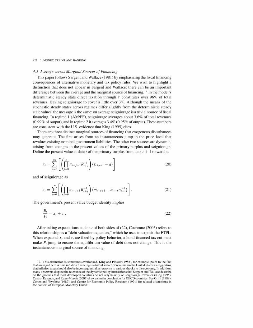
5.2 Impacts of Policy Shocks in Regime 2 (PM/AF)

Regime 2 policy behavior corresponds to the standard FTPL exercise: both taxesand the nominal interest rate are exogenous.

Tax shocks. A permanent regime 2 is the canonical FTPL exercise. Fixed future taxesand constant current and future interest rates mean that a tax cut cannot be financedby future revenues. At initial interest rates and prices, agents feel wealthier and try toincrease their consumption paths. This increase in demand drives up the current pricelevel until the value of debt is returned to its original level and agents are happy with


0 5 10 152

2.5

3

3.5

4

4.5

π

ψθ

0 5 10 150.37

0.375

0.38

0.385

0.39

0.395

b

0 5 10 156.7

6.8

6.9

7

7.1

7.2

R

0 5 10 150.245

0.25

0.255

0.26

τ

0 5 10 15

0

2

4

6

8

M g

row

th

0 5 10 15

0

2

4

6

8

B g

row

th

5 10 150.145

0.15

0.155

0.16

0.165

PV

sur

plus

0 5 10 150.215

0.22

0.225

0.23

0.235

PV

sei

gnio

rage

FIG. 3. Impacts of Policy Shocks Conditional on Regime 2 (PM/AF).

NOTE: For the tax shock, ψ , the figure plots deviations of E[xt+ j |{St+ j = 2, ψt < 0, θt = 0, j ≥ 0}] from steady stateand for the monetary policy shock, θ , the figure plots analogous deviations of E[xt+ j |{St+ j = 2, ψt = 0, θt < 0, j ≥ 0}].Because the shocks are i.i.d., their expected future values are zero.

their initial consumption plans. By fixing the interest rate, monetary policy preventsthe tax shock from propagating.

Regime switching does not alter the fixed-regime results (Figure 3). The currentinflation rate jumps to devalue the newly issued nominal debt; on the margin, the full


tax cut is financed by a contemporaneous jump in the price level. An unchanged valueof debt is consistent with unchanged present values of taxes and seigniorage. Moneygrowth reacts passively to the higher price level to ensure the money market clearsat the fixed nominal interest rate. These effects coincide with those under a fixedPM/AF regime because even though agents impute a positive probability to a passivetax policy and a Taylor rule in the future, unchanged real debt and an unchangedpresent value of surpluses are consistent with such a switch in rules. Indeed, thedecision rules as a function of ψ t are identical across fixed- and switching regimesetups.15

Monetary shocks. When regime 2 is fixed, a monetary policy shock at time t lowersthe nominal interest rate and induces offsetting portfolio substitutions by agents outof debt and into money. With agents’ budget sets unperturbed by the shock, there isno change in aggregate demand or inflation initially. The lower nominal interest ratecreates an expectation of lower future inflation and, therefore, seigniorage revenues(supporting the drop in the value of debt). How is the lower expected inflation realized?Although initial changes in real balances and real debt offset each other, the drop inRt makes financial wealth, wt, lower at the beginning of period t + 1. This reducesdemand and inflation in that period.

When regime can switch, surprise monetary easing produces a similar patternof impacts. The only difference is the small contemporaneous uptick in inflation(Figure 3), which arises because agents impute a positive probability to switching toregime 1 (AM/PF), where expansionary monetary policy raises inflation.

With monetary policy in this model couched in terms of an interest rate rule, theexpansionary monetary shock produces a sizeable “price puzzle.” As we explorein Section 7, this pattern of correlation offers an explanation for the “price puzzle”findings in the monetary VAR literature.

6. EXPLORING THE PARAMETER SPACE

This section considers alternative parameter settings across two dimensions of theparameter space. First, we vary regime duration and report the sensitivity of inflationto taxes when regime 1 (AM/PF) prevails. The benchmark settings for the PM/AFregime assume the monetary authority sets interest rates independently of inflation,implying tax reductions are financed entirely by a contemporaneous inflation tax (as inthe FTPL). The second dimension we explore is to allow monetary policy to respondweakly to inflation.

15. Daniel (2003) considers a once-and-for-all probabilistic shift in tax policy from being stronglyresponsive to debt to being exogenous. She maintains that monetary policy pegs the nominal interest rateforever. In the present setup, Daniel is assuming the tax rule can switch from regime 1 [γ 1(1) > 0] toregime 2 [γ 1(2) = 0], while monetary policy is always in regime 2 [α1(1) = α1(2) = 0]. She shows thatas long as the probability is positive that taxes will be exogenous in the future, fiscal policy determines theprice level. Because the nominal rate is pegged, there is no mechanism in Daniel’s model by which a taxshock can be propagated. Even if taxes are currently in regime 1, therefore, their impacts are those that thepresent work attributes to regime 2: a one-time change in the price level that revalues debt.


0 0.005 0.01 0.015 0.02

0

0.2

0.4

0.6

0.8

1

∆π

t

ψt

λ=0

λ=.25

λ=.5

λ=.75 λ=1

FIG. 4. Regime 1 (AM/PF).

NOTE: Contemporaneous impact of taxes on inflation as a function of λ, proportion of time spent in regime 1 in the ergodicdistribution. Computed as described in Figure 2.

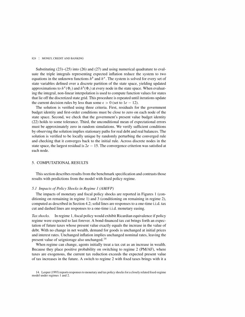
6.1 An Active Monetary/Passive Fiscal Regime

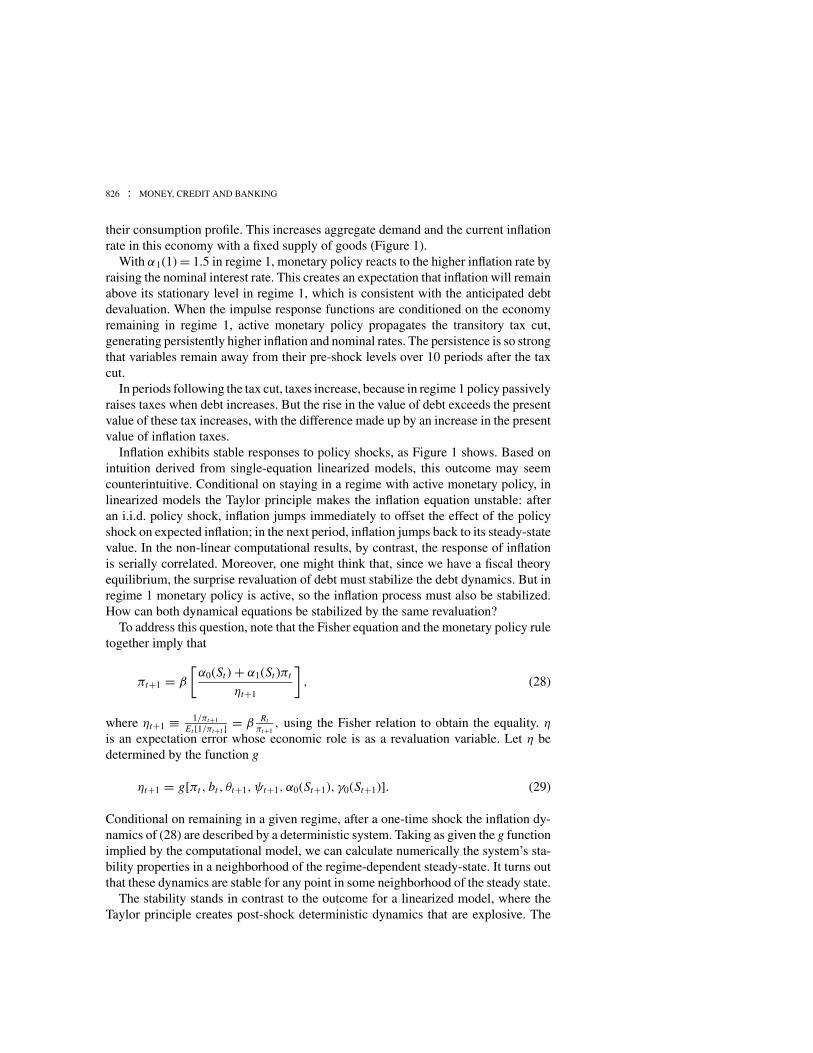
As Section 5 demonstrated, agents’ expectations that regime will switch in thefuture play a crucial role in determining the impacts of policy disturbances. Here weexplore how regime duration affects the result that tax cuts generate wealth effects inregime 1. The expected duration of a regime is given by

E[d j |St = j] = 1

1 − p j j,

for j = {1, 2} and dj = T − t , where St = St+1 = ··· = St+T = j and St+T +1 �= j .The benchmark specification assumes that both regimes are relatively persistent: p11

> .5 and p22 > .5.The degree to which tax shocks affect inflation in an AM/PF regime depends on the

transition matrix. Figure 4 illustrates how the impact of a tax cut on inflation increasesas p11 → 0 and p22 → 1. Each decision rule represents different probabilities in thetransition matrix, where

λ = E [d1|St = 1]

E [d1|St = 1] + E [d2|St = 2]


1 2 3 4 5 6 70

0.1

0.2

0.3

0.4

0.5

0.6

0.7

0.8

∆π

t

λ=0

λ=.25

λ=.5

λ=.75

FIG. 5. Regime 1 (AM/PF).

NOTE: Response of inflation to tax cut in period 2 as a function of λ, proportion of time spent in regime 1 in the ergodicdistribution. Computed as described in Figure 1.

represents the proportion of time spent in the AM/PF regime in the ergodic distri-bution. As the expected proportion of time spent in the PM/AF regime increases,the inflation effects of tax disturbances increase because agents expect to switch tothe PM/AF regime in the future and then remain there longer relative to the AM/PFregime.

As Figure 5 illustrates, the transition matrix affects the sensitivity of inflation to atax cut. The paths for inflation condition on the AM/PF regime and use that regime’ssteady state as the baseline; the tax cut occurs in period 2. As agents expect to spendrelatively more time in the PM/AF regime, a tax cut generates a larger increase ininflation on impact and increases the variance of inflation. The larger increase onimpact arises from the expectation of a regime change to a more persistent PM/AFregime in the near future, which creates a lower expected present value of direct taxesrelative to a scenario where the AM/PF regime is highly persistent.

6.2 A Passive Monetary/Active Fiscal Regime

In the fixed-regime model, with exogenous taxes and a pegged interest rate, therevaluation of nominal debt following an i.i.d. shock to taxes occurs instantaneously.But even when regime is fixed, transitory tax shocks can generate serially correlatedchanges in inflation if the monetary authority responds weakly to inflation (α1 > 0).


1 2 3 4 5 6 70

0.005

0.01

0.015

0.02

0.025

∆ ln

(PV

of S

eign

iora

ge)

α=.1

α=.2

α=.3

α=.4

FIG. 6. Fixed Regime (PM/AF).

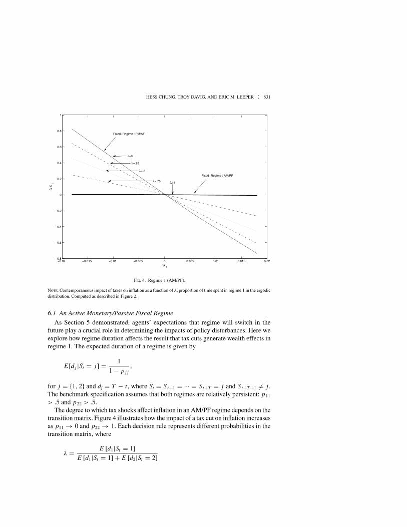
NOTE: Response of the present value of seigniorage to tax cut in period 2 as a function of the monetary policy responseof the interest rate to inflation. Computed as described in Figure 2, conditional on St = 2, with p11 = 0, p22 = 1, andα1(2) = 0.1, 0.2, 0.3, 0.4.

This prevents the complete devaluation of nominal debt from occurring in the periodof the tax shock. Instead, a tax cut is financed by issuing debt that will be repaid withinflation taxes spread over future periods.

As α1 increases, the monetary authority responds more aggressively to inflation andthe tax cut causes a larger increase in the interest rate and a smaller contemporaneousrise in inflation. The higher interest rate, along with a higher real value of debt (dueto a smaller jump in the current price level), induces substitution from real balancesto bonds. As α1 increases, so must the present value of seigniorage following a taxcut. However, regardless of the value of α1 in the fixed-regime model, the persistencein inflation is quite weak, as the present value of future seigniorage returns to itsinitial level relatively quickly. These effects are illustrated in Figure 6 for a tax cut inperiod 2.

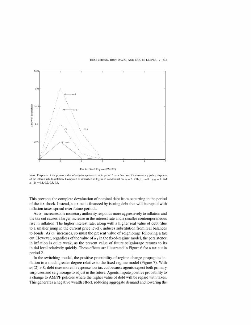
In the switching model, the positive probability of regime change propagates in-flation to a much greater degree relative to the fixed-regime model (Figure 7). Withα1(2) > 0, debt rises more in response to a tax cut because agents expect both primarysurpluses and seigniorage to adjust in the future. Agents impute positive probability toa change to AM/PF policies where the higher value of debt will be repaid with taxes.This generates a negative wealth effect, reducing aggregate demand and lowering the


1 2 3 4 5 6 70

0.005

0.01

0.015

0.02

0.025

∆ ln

(PV

of S

eign

iora

ge)

α=.1

α=.2

α=.3

α=.4

FIG. 7. Regime 2 (PM/AF).

NOTE: Response of the present value of seigniorage to tax cut in period 2 as a function of the monetary policy responseof the interest rate to inflation. Computed as described in Figure 6, with p11 = p22 = 0.85 and α1(2) = 0.1, 0.2, 0.3, 0.4.

rate of inflation relative to the fixed regime model. These effects are in place until thepolicy regime changes.

7. SOME EMPIRICAL IMPLICATIONS

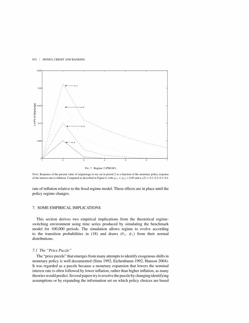
This section derives two empirical implications from the theoretical regime-switching environment using time series produced by simulating the benchmarkmodel for 100,000 periods. The simulation allows regime to evolve accordingto the transition probabilities in (18) and draws (θ t , ψ t ) from their normaldistributions.

7.1 The “Price Puzzle”

The “price puzzle” that emerges from many attempts to identify exogenous shifts inmonetary policy is well documented (Sims 1992, Eichenbaum 1992, Hanson 2004).It was regarded as a puzzle because a monetary expansion that lowers the nominalinterest rate is often followed by lower inflation, rather than higher inflation, as manytheories would predict. Several papers try to resolve the puzzle by changing identifyingassumptions or by expanding the information set on which policy choices are based


1 2 3 4 5 6 7 8 9 100

0.05

0.1

0.15

0.2

π

1 2 3 4 5 6 7 8 9 100

0.05

0.1

0.15

0.2

R

FIG. 8. Responses to a Nominal Interest Rate Innovation.

NOTE: Data simulated from the regime-switching model. Estimated from a bivariate VAR using simulated inflation andnominal interest rate data. Results from a Choleski decomposition in the order of inflation-nominal rate.

(Gordon and Leeper 1994, Leeper, Sims, and Zha 1996, Christiano, Eichenbaum, andEvans 1999, Bernanke, Boivin, and Eliasz 2005, Leeper and Roush 2003).

Another reaction has been that lower inflation following a lower interest rate isnot a puzzle at all. To the extent that firms must borrow to finance wage bills andnew investment, lower interest rates reduce the costs of production and can lead nat-urally to lower inflation, at least for some period (Barth and Ramey 2002, Christiano,Eichenbaum, and Evans 2005).

As suggested in Section 5, a positive correlation between the interest rate and futureinflation is also a natural outcome of the switching model. It appears subtly underregime 1 (AM/PF) and forcefully under regime 2 (PM/AF). We now show that iftime series data were generated by this setup, one should expect to find that positiveinterest rate innovations predict higher inflation.

Figure 8 shows the responses of inflation and the nominal interest rate to an or-thogonalized innovation in the nominal rate. Ordering inflation before the interest rateis consistent with much of the VAR work, which treats inflation as predetermined,and is also consistent with estimates of the Taylor rule, which regress the nominalrate on inflation (and potentially other variables). Although the policy disturbances


1 2 3 4 5 6 7 8 9 10

0

0.1

0.2

0.3

0.4

0.5

Sur

plus

1 2 3 4 5 6 7 8 9 10

0

Liab

ilitie

s

FIG. 9. Responses to a Surplus Innovation.

NOTE: Data simulated from the regime-switching model. Estimated from a bivariate VAR using simulated governmentsurplus and liabilities data. Results from a Choleski decomposition in the order of surplus liabilities.

are i.i.d. and the monetary policy rule is purely contemporaneous, the interest ratedisplays substantial serial correlation. Inflation rises sharply in the short run, andremains above its initial level for 10 periods.

The model’s results are consistent with the Hanson’s (2004) careful analysis. Hefinds that the “price puzzle” cannot be solved by the conventional method of addingcommodity prices to the Fed’s information set. And more to the point for the presentwork, Hanson finds that the “puzzle” is more pronounced in the period 1960–79. ButFavero and Monacelli (2003) identify that period as one where monetary policy waspassive and fiscal policy was active. As Figure 3 shows, the model predicts preciselythis outcome when conditioning on PM/AF.

7.2 Surplus-Debt Regressions

A number of authors have computed regressions of budget surpluses and govern-ment debt to draw inferences about the source of fiscal financing (Canzoneri, Cumby,and Diba 2001, Bohn 1998, Janssen, Nolan, and Thomas 2002). Canzoneri, Cumby,and Diba (CCD), for example, estimate a bivariate VAR with the government surplus


and total liabilities.16 Their Figure 3 (p. 1228) reports that a positive innovation in thesurplus is followed by persistently lower liabilities and a surplus that is significantlypositive for only two periods. They argue that a Ricardian interpretation of the datais “more plausible” than is a non-Ricardian one, as the increase in the surplus is usedto retire debt.

Simulated data from the regime-switching model produce a pattern of correlationstrikingly similar to the top panel of CCD’s figure. A positive innovation to the surplusproduces an immediate and persistent decline in liabilities (Figure 9). Of course, asFigure 1 makes clear, even conditional on current tax policy being Ricardian, taxshocks always generate wealth effects and Ricardian equivalence fails to hold.

Our setup is completely straightforward and plausible. Both a reading of Americantax history over CCD’s sample period and the corroborating formal statistical evidencethat Favero and Monacelli (2003) present support the view that monetary and fiscalpolicy regimes have switched in a manner that our setup aims to capture.

8. CONCLUDING REMARKS

In most countries monetary and fiscal authorities cannot credibly commit to alwaysfollow either active monetary policy and passive fiscal policy or passive monetarypolicy and active fiscal policy. If, as a consequence, private agents place probabilitymass on both kinds of regimes, then something like the regime-switching environ-ment that we model will apply. That environment makes wealth effects—from bothmonetary and tax policy disturbances—important components of policy impacts.

The implications of this switching setup raise some doubts about two pillars ofrecent policy analysis. First, because tax changes have wealth effects, even if theprevailing regime combines the Taylor principle for monetary policy with taxes thatrespond strongly to debt, Ricardian equivalence may be a misleading benchmark.Second, if the Taylor principle holds in only one regime, it can actually be destabilizingin the sense that it propagates disturbances and can increase the variance of aggregatedemand and inflation.

There are several dimensions along which to extend the current framework. Isit possible for both policy authorities to act passively in one regime, yet have theprice level uniquely determined? The analytical example in Section 2 shows this ispossible. The current computational approach must be modified to deliver and ap-propriately characterize a solution with multiple equilibria or sunspots, as Lubik andSchorfheide (2003) have done for linear models. The second extension addresses thequestion: how “big” are the fiscal effects when the current regime is AM/PF? Toaddress this, we need a carefully calibrated model with frictions, possibly of the kindin the workhorse New Keynesian model extended to include long-term governmentdebt as in Cochrane (2001). In the New Keynesian model monetary policy has more

16. The surplus is defined to include seigniorage and total liabilities are the sum of net governmentdebt and the monetary base.


conventional macro effects, in addition to the fiscal financing effects this paper an-alyzes. With such a model in hand, we could also extract a more complete set ofempirical implications.

A third extension is more ambitious: endogenizing regime change. As suggestedin the introduction, it is not very satisfactory to make regime a deterministic func-tion of the state of the economy because both the timing and the nature of regimechange are uncertain. More sophisticated modeling of regime change, including bothendogenous and exogenous components and possibly time-varying transition prob-abilities, is likely to be a productive direction for future research.

LITERATURE CITED

Andolfatto, D., and P. Gomme. (2003) “Monetary Policy Regimes and Beliefs.” InternationalEconomic Review, 44:1, 1–30.

Andolfatto, D., S. Hendry, and K. Moran. (2002) “Inflation Expectations and Learning aboutMonetary Policy.” Bank of Canada Working Paper No. 2002-30.

Auerbach, A. J. (2002) “Is There a Role for Discretionary Fiscal Policy?” In Rethink-ing Stabilization Policy: Proceedings of a Symposium Sponsored by the Federal ReserveBank of Kansas City, pp. 109–50. Federal Reserve Bank of Kansas City, Jackson HoleSymposium.

Barth, M. J., and V. A. Ramey. (2002) “The Cost Channel of Monetary Transmission.” InNBER Macroeconomics Annual 2001, Vol. 16(1), edited by B. S. Bernanke and K. Rogoff,pp. 199–240. Cambridge, MA: MIT Press.

Benhabib, J., S. Schmitt-Grohe, and M. Uribe. (2001a) “Monetary Policy and Multiple Equi-libria.” American Economic Review, 91:1, 167–86.

Benhabib, J., S. Schmitt-Grohe, and M. Uribe. (2001b) “The Perils of Taylor Rules.” Journalof Economic Theory, 96:1–2, 40–69.

Benhabib, J., S. Schmitt-Grohe, and M. Uribe. (2002) “Avoiding Liquidity Traps.” Journal ofPolitical Economy, 110:3, 535–63.

Bernanke, B. S., J. Boivin, and P. Eliasz. (2005) “Measuring the Effects of Monetary Policy:A Factor-Augmented Vector Autoregressive (FAVAR) Approach.” Quarterly Journal ofEconomics, 120:1, 387–422.

Bernanke, B. S., and I. Mihov. (1998) “Measuring Monetary Policy.” Quarterly Journal ofEconomics, 113:3, 869–902.

Bohn, H. (1998) “The Behavior of U.S. Public Debt and Deficits.” Quarterly Journal of Eco-nomics, 113:3, 949–63.

Bryant, R. C., P. Hooper, and C. L. Mann. (eds.) (1993) Evaluating Policy Regimes: NewResearch in Empirical Macroeconomics. Washington, DC: The Brookings Institution.

Canzoneri, M. B., R. E. Cumby, and B. T. Diba. (2001) “Is the Price Level Determined by theNeeds of Fiscal Solvency?” American Economic Review, 91:5, 1221–38.

Castro, R., C. Resende, and F. J. Ruge-Murcia. (2003) “The Backing of Government Debt andthe Price Level.” Manuscript, Universite de Montreal.

Centre for Economic Policy Research. (1991) Monitoring European Integration: The Makingof Monetary Union. CEPR Annual Report, London.


Christiano, L. J., M. Eichenbaum, and C. L. Evans. (1999) “Monetary Policy Shocks: WhatHave We Learned and to What End?” In Handbook of Macroeconomics, Vol. 1A, edited byJ. B. Taylor and M. Woodford, pp. 65–148. Amsterdam: Elsevier Science.

Christiano, L. J., M. Eichenbaum, and C. L. Evans. (2005) “Nominal Rigidities and the DynamicEffects of a Shock to Monetary Policy.” Journal of Political Economy, 113:1, 1–45.

Clarida, R., J. Gali, and M. Gertler. (2000) “Monetary Policy Rules and MacroeconomicStability: Evidence and Some Theory.” Quarterly Journal of Economics, 115:1, 147–80.

Cochrane, J. H. (1998) “A Frictionless View of U.S. Inflation.” In NBER Macroeconomics An-nual 1998, Vol. 13(1), edited by B. S. Bernanke and J. J. Rotemberg, pp. 323–84. Cambridge,MA: MIT Press.

Cochrane, J. H. (2001) “Long Term Debt and Optimal Policy in the Fiscal Theory of the PriceLevel.” Econometrica, 69:1, 69–116.

Cochrane, J. H. (2005) “Money as Stock.” Journal of Monetary Economics, 52:3, 501–28.

Cogley, T., and T. J. Sargent. (2002) “Evolving Post-World War II U.S. Inflation Dynamics.”In NBER Macroeconomics Annual 2001, Vol. 16(1), edited by B. S. Bernanke and J. J.Rotemberg. Cambridge, MA: MIT Press.

Cogley, T., and T. J. Sargent. (2005) “Drifts and Volatilities: Monetary Policies and Outcomesin the Post WWII U.S.” Review of Economic Dynamics, 8:2, 262–302.

Cohen, D., and C. Wyplosz. (1989) “The European Monetary Union: An Agnostic Evaluation.”In Macroeconomic Policies in an Interdependent World, edited by R. C. Bryant, D. A. Currie,J. Frankel, P. Masson, and R. Portes, pp. 311–37. Washington, DC: The Brookings Institution.

Coleman, W. J., II. (1991) “Equilibrium in a Production Economy with an Income Tax.”Econometrica, 59:4, 1091–1104.

Cooley, T. F., S. F. LeRoy, and N. Raymon. (1982) “Modeling Policy Interventions.” Mimeo,University of California, Santa Barbara.

Cooley, T. F., S. F. LeRoy, and N. Raymon. (1984) “Econometric Policy Evaluation: Note.”American Economic Review, 74:3, 467–70.

Daniel, B. C. (2003) “Fiscal Policy, Price Surprises, and Inflation.” Manuscript, SUNY Albany.

Davig, T. (2003) “Regime-Switching Fiscal Policy in General Equilibrium.” Manuscript, TheCollege of William and Mary.

Davig, T. (2004) “Regime-Switching Debt and Taxation.” Journal of Monetary Economics,51:4, 837–59.

Davig, T., and E. M. Leeper. (Forthcoming-a) “Fluctuating Macro Policies and the FiscalTheory.” NBER Macroeconomics Annual 2006.

Davig, T., and E. M. Leeper. (Forthcoming-b) “Generalizing the Taylor Principle.” AmericanEconomic Review.

Davig, T., E. M. Leeper, and H. Chung. (2004) “Monetary and Fiscal Policy Switching.” NBERWorking Paper No. 10362.

Eichenbaum, M. (1992) “Comment on ‘Interpreting the Macroeconomic Time Series Facts:The Effects of Monetary Policy.’ ” European Economic Review, 36, 1001–11.

Favero, C. A., and T. Monacelli. (2003) “Monetary-Fiscal Mix and Inflation Performance:Evidence from the US.” CEPR Discussion Paper No. 3887.

Gallant, A. R., P. E. Rossi, and G. Tauchen. (1993) “Nonlinear Dynamic Structures.” Econo-metrica, 61:4, 871–907.


Gordon, D. B., and E. M. Leeper. (1994) “The Dynamic Impacts of Monetary Policy: AnExercise in Tentative Identification.” Journal of Political Economy, 102, 1228–47.

Grilli, V. (1989) “Seigniorage in Europe.” In A European Central Bank? Perspectives onMonetary Unification after Ten Years of the EMS, edited by M. DeCecco, and A. Giovannini,pp. 53–79. Cambridge: Cambridge University Press.

Hanson, M. S. (2004) “The ”Price Puzzle‘ Reconsidered.” Journal of Monetary Economics,51:7, 1385–413.

Hanson, M. S. (2006) “Varying Monetary Policy Regimes: A Vector Autoregressive Investi-gation.” Journal of Economics and Business, 58, 407–27.

Heller, W. W. (1967) New Dimensions of Political Economy. New York: Norton.

Janssen, N., C. Nolan, and R. Thomas. (2002) “Money, Debt and Prices in the UK 1705–1996.”Economica, 69:275, 461–79.

King, M. (1995) “Commentary: Monetary Policy Implications of Greater Fiscal Discipline.” InBudget Deficits and Debt: Issues and Options, pp. 171–83. Federal Reserve Bank of KansasCity, Jackson Hole Symposium.

King, R. G., and C. I. Plosser. (1985) “Money, Deficits, and Inflation.” In Carnegie-RochesterConference Series on Public Policy, Vol. 22, pp. 147–96. Amsterdam: North-Holland.

Leeper, E. M. (1991) “Equilibria Under ‘Active’ and ‘Passive’ Monetary and Fiscal Policies.”Journal of Monetary Economics, 27:1, 129–47.

Leeper, E. M. (1993) “The Policy Tango: Toward a Holistic View of Monetary and FiscalEffects.” Federal Reserve Bank of Atlanta Economic Review, 78:4, 1–27.

Leeper, E. M., and J. E. Roush. (2003) “Putting ‘M’ Back in Monetary Policy.” Journal ofMoney, Credit, and Banking, 35(6, Part 2), 1217–56.

Leeper, E. M., C. A. Sims, and T. Zha (1996) “What Does Monetary Policy Do?” BrookingsPapers on Economic Activity, 2, 1–63.

Leeper, E. M., and T. Yun. (2006) “The Fiscal Theory of the Price Level: Background andBeyond.” International Tax and Public Finance, 13, 373–409.

Leeper, E. M., and T. Zha. (2003) “Modest Policy Interventions.” Journal of Monetary Eco-nomics, 50:8, 1673–700.

Loyo, E. (1999) “Tight Money Paradox on the Loose: A Fiscalist Hyperinflation.” Manuscript,Harvard University.

Lubik, T. A., and F. Schorfheide. (2003) “Computing Sunspot Equilibria in Linear RationalExpectations Models.” Journal of Economic Dynamics and Control, 28:2, 273–85.

Lubik, T. A., and F. Schorfheide (2004) “Testing for Indeterminacy: An Application to U.S.Monetary Policy.” American Economic Review, 94, 190–217.

Lucas, Jr., R. E. (1976) “Econometric Policy Evaluation: A Critique.” In Carnegie-Rochester Conference Series on Public Policy, Vol. 1, pp. 104–30. Amsterdam:North-Holland.

Mackowiak, B. (2006) “Macroeconomic Regime Switching and Speculative Attacks.”Manuscript, Humbolt University.

Obstfeld, M., and K. Rogoff. (1983) “Speculative Hyperinflations in Maximizing Models: CanWe Rule Them Out?” Journal of Political Economy, 91, 675–87.

Ohanian, L. E. (1997) “The Macroeconomic Effects of War Finance in the United States: WorldWar II and the Korean War.” American Economic Review, 87:1, 23–40.


Pechman, J. A. (1987) Federal Tax Policy, 5th ed. Washington, DC: The Brookings Institution.

Poterba, J. M. (1994) “Federal Budget Policy in the 1980s.” In American Economic Policy inthe 1980s, edited by M. Feldstein, pp. 235–70. Chicago: University of Chicago Press.

Sala, L. (2004) “Testing the Fiscal Theory of the Price Level: Identifying Restrictions andEmpirical Evidence.” IGIER Working Paper No. 257.

Sargent, T. J. (1999) The Conquest of American Inflation. Princeton, NJ: Princeton UniversityPress.

Sargent, T. J., and N. Wallace. (1981) “Some Unpleasant Monetarist Arithmetic.” FederalReserve Bank of Minneapolis Quarterly Review, 5, 1–17.

Schorfheide, F. (2005) “Learning and Monetary Policy Shifts.” Review of Economic Dynamics,8:2, 392–419.

Sidrauski, M. (1967) “Rational Choice and Patterns of Growth in a Monetary Economy.”American Economic Review Papers and Proceedings, 57:2, 534–44.

Sims, C. A. (1986) “Are Forecasting Models Usable for Policy Analysis?” Federal ReserveBank of Minneapolis Quarterly Review, 10, 1–16.

Sims, C. A. (1987) “A Rational Expectations Framework for Short-Run Policy Analysis.”In New Approaches to Monetary Economics, edited by W. A. Barnett and K. J. Singleton,pp. 293–308. Cambridge UK: University Press.

Sims, C. A. (1988) “Identifying Policy Effects.” In Empirical Macroeconomics for Interde-pendent Economics, edited by R. C. Bryant, D.W. Henderson, G. Holtham, P. Hooper, andS. A. Symansky, pp. 308–21. Washington, DC: The Brookings Institution.

Sims, C. A. (1992) “Interpreting the Macroeconomic Time Series Facts: The Effects of Mon-etary Policy.” European Economic Review, 36, 975–1000.

Sims, C. A. (1994) “A Simple Model for Study of the Determination of the PriceLevel and the Interaction of Monetary and Fiscal Policy.” Economic Theory, 4:3,381–99.

Sims, C. A. (1997) “Fiscal Foundations of Price Stability in Open Economies.” Manuscript,Yale University.

Sims, C. A. (1998) “The Role of Interest Rate Policy in the Generation and Propagation ofBusiness Cycles: What Has Changed Since the ’30s?” In Beyond Shocks: What CausesBusiness Cycles? edited by J. C. Fuhrer and S. Schuh, pp. 121–60. Boston: Federal ReserveBank of Boston.

Sims, C. A., and T. Zha. (2006) “Were There Regime Switches in US Monetary Policy?”American Economic Review, 96:1, 54–81.

Stein, H. (1996) The Fiscal Revolution in America, 2nd rev. ed. Washington, DC: AEI Press.

Steuerle, E. (2002) “Tax Policy from 1990 to 2001.” In American Economic Policy in the 1990s,edited by J. Frankel and P. Orszag, pp. 139–69. Cambridge, MA: MIT Press.

Taylor, J. B. (1993) “Discretion versus Policy Rules in Practice.” In Carnegie-Rochester Con-ference Series on Public Policy, Vol. 39, pp. 195–214. Amesterdam: North Holland.

Taylor, J. B. (1996) “Monetary Policy Implications of Greater Fiscal Discipline.” In BudgetDeficits and Debt: Issues and Options, pp. 151–70. Federal Reserve Bank of Kansas City,Jackson Hole Symposium.

Taylor, J. B. (1999a) “An Historical Analysis of Monetary Policy Rules.” In Monetary PolicyRules, edited by J. B. Taylor, pp. 319–41. Chicago: University of Chicago Press.

Taylor, J. B. (ed.) (1999b) Monetary Policy Rules. Chicago: University of Chicago Press.


Taylor, J. B. (2000) “Reassessing Discretionary Fiscal Policy.” Journal of Economic Perspec-tives, 14:3, 21–36.

Weil, P. (2002) “Reflections on the Fiscal Theory of the Price Level.” Manuscript, ECARES.

Woodford, M. (1995) “Price-Level Determinacy Without Control of a Monetary Aggregate.”In Carnegie-Rochester Conference Series on Public Policy, Vol. 43, pp. 1–46. Amsterdam:North-Holland.

Woodford, M. (1998a) “Public Debt and the Price Level.” Manuscript, Princeton University.

Woodford, M. (1998b) “Comment on Cochrane’s ‘A Frictionless View of U.S. Inflation’.”In NBER Macroeconomics Annual 1998, edited by B. S. Bernanke and J. J. Rotemberg,pp. 390–419. Cambridge, MA: MIT Press.

Yang, S.-C. S. (Forthcoming) “Tentative Evidence of Tax Foresight.” Economics Letters.

Documents

Monetary and Fiscal Policy Switching - Indiana …mypage.iu.edu/~eleeper/Papers/DavigLeeperChungJMCBFinal.pdf · HESS CHUNG TROY DAVIG ERIC M. LEEPER Monetary and Fiscal Policy Switching